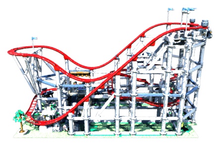
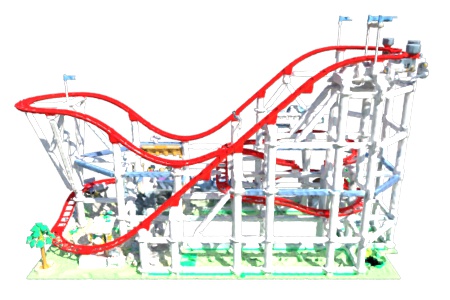
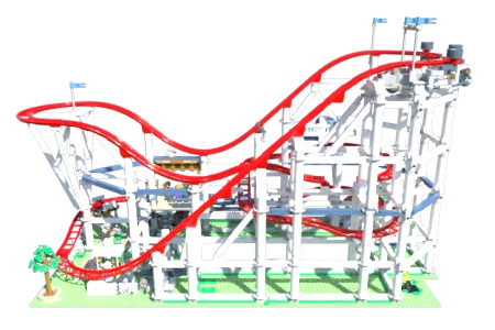
Shape, Light, and Material Decomposition from Images using Monte Carlo Rendering and Denoising
Abstract
Recent advances in differentiable rendering have enabled high-quality reconstruction of 3D scenes from multi-view images. Most methods rely on simple rendering algorithms: pre-filtered direct lighting or learned representations of irradiance. We show that a more realistic shading model, incorporating ray tracing and Monte Carlo integration, substantially improves decomposition into shape, materials & lighting. Unfortunately, Monte Carlo integration provides estimates with significant noise, even at large sample counts, which makes gradient-based inverse rendering very challenging. To address this, we incorporate multiple importance sampling and denoising in a novel inverse rendering pipeline. This improves convergence and enables gradient-based optimization at low sample counts. We present an efficient method to jointly reconstruct geometry (explicit triangle meshes), materials, and lighting, which substantially improves material and light separation compared to previous work. We argue that denoising can become an integral part of high quality inverse rendering pipelines.
1 Introduction
Differentiable rendering shows great promise for accurate multi-view 3D reconstruction from image observations. NeRF [39] use differentiable volume rendering to create high quality view interpolation through neural, density-based light-fields. Surface-based methods apply signed distance fields [43, 47, 68, 62, 73] or triangle meshes [41, 54] to capture high quality geometry. Recent work [6, 41, 75] further decompose these representations into geometry, material, and environment light.
Most aforementioned methods rely on appearance baked into neural light fields or apply simple shading models. Typically, direct lighting without shadows is considered, combined with pre-filtered representations of environment lighting [41, 73]. Some methods account for shadowing and indirect illumination [6, 75, 77], but often lock the geometry optimization when sampling the shadow term, or rely on learned representations of irradiance. While results are impressive, the deviations from physically-based shading models makes it harder for these methods to plausibly disentangle shape, material and lighting, as shown in Figure 1.
|
||||||||
|
||||||||
In theory, it is straightforward to replace the rendering engines of these 3D reconstruction methods with photorealistic differentiable renderers [31, 36, 46, 45, 71, 72] and optimize in a setting with more accurate light simulation, including global illumination effects. In practice, however, the noise in multi-bounce Monte Carlo rendering makes gradient-based optimization challenging. Very high sample counts are required, which result in intractable iteration times.
In this paper, we bridge the gap between current multi-view 3D reconstruction and physically-based differentiable rendering, and demonstrate high-quality reconstructions at competitive runtime performance. We attack the challenging case of extracting explicit triangle meshes, PBR materials and environment lighting from a set of multi-view images, in a format directly compatible with current DCC tools and game engines. For improved visual fidelity, we compute direct illumination using Monte Carlo integration with ray tracing, and add several techniques to combat the increased noise levels. By carefully trading variance for bias, we enable efficient gradient-based optimization in a physically-based inverse rendering pipeline. Compared to previous 3D reconstruction methods, our formulation primarily improves material and light separation.
Concretely, we reduce variance by combining multiple importance sampling [58] and differentiable denoisers. We evaluate both neural denoisers [2, 10, 22] and cross-bilateral filters [52] in our pipeline. Furthermore, we decompose the rendering equation into albedo, demodulated diffuse lighting and specular lighting, which enable precise regularization to improve light and material separation.
2 Previous Work
Neural methods for multi-view reconstruction
These methods fall in two categories: implicit or explicit scene representations. NeRF [39] and follow-ups [38, 42, 49, 74, 64, 15, 40, 50, 69, 66], use volumetric representations and compute radiance by ray marching through a neurally encoded 5D light field. While achieving impressive results on novel view synthesis, geometric quality suffers from the ambiguity of volume rendering [74]. Surface-based rendering methods [43, 47, 68, 62] optimizing the underlying surface directly using implicit differentiation, or gradually morph from a volumetric representation into a surface representation. Methods with explicit representation estimate 3D meshes from images, where most approaches assume a given mesh topology [35, 11, 12], but recent work also include topology optimization [34, 14, 54, 41].
BRDF and lighting estimation
To estimate surface radiometric properties from images, previous work on BTF and SVBRDF estimation rely on special viewing configurations, lighting patterns or complex capturing setups [30, 16, 17, 18, 65, 5, 8, 53, 20]. Recent methods exploit neural networks to predict BRDFs from images [13, 19, 32, 33, 44, 37]. Differentiable rendering methods [35, 11, 76, 12, 21] learn to predict geometry, SVBRDF and, in some cases, lighting via photometric loss.
Most related to our work are neural 3D reconstruction methods with intrinsic decomposition of shape, materials, and lighting from images [6, 7, 41, 73, 75, 77]. Illumination is represented using mixtures of spherical Gaussians [6, 41, 73, 77], pre-filtered approximations [7, 41], or low resolution environment maps [75]. When the shadowing term is accounted for [75], optimization is split into two passes where geometry is locked before the shadow term is sampled. Other approaches represent indirect illumination with neural networks [63, 77].
Image denoisers
Denoisers are essential tools in both real-time- and production renderers. Traditionally, variants of cross-bilateral filters are used [78], which require scene-specific manual adjustments. More recently, neural denoisers [2, 10, 22] trained on large datasets have shown impressive quality without the need for manual tuning, and are now incorporated in most production renderers. We directly incorporate differentiable versions of these denoisers in our pipeline. We are currently unaware of image denoisers applied in differentiable rendering, but we see a lot of potential for denoisers in physically-based inverse rendering going forward.
3 System
We target the challenging task of joint optimization of shape, material and environment lighting from a set of multi-view images with known foreground segmentation masks and camera poses. Our goal is to use physically-based rendering techniques to improve the intrinsic decomposition of lighting and materials, producing assets that can be relit, edited, animated, or used in simulation. As a proof-of-concept, we extend a recent approach, nvdiffrec [41], which targets the same optimization task (shape, materials and environment lighting). Notably, they directly optimize a triangular 3D model, which has obvious benefits: it is easy to import and modify the reconstructed models in existing DCC tools, and a triangular representation can exploit hardware-accelerated differentiable rasterization [28]. In our setting, triangular 3D models also means we can leverage hardware-accelerated ray-tracing for efficient shadow tests. nvdiffrec reports competitive results on view interpolation, material reconstruction, and relighting, and we will use their pipeline as a baseline in our evaluations.

Our system is summarized in Figure 2. A triangular mesh with arbitrary topology is optimized from a set of images through 2D supervision. Geometry is represented by a signed distance field defined on a three-dimensional grid and reduced to a triangular surface mesh through deep marching tetrahedra (DMTet) [54]. Next, the extracted surface mesh is rendered in a differentiable renderer, using the physically-based (PBR) material model from Disney [9]. This material model combines a diffuse term with an isotropic, specular GGX lobe [61]. A tangent space normal map is also included to capture high frequency shading detail. Finally, the rendered image is evaluated against a reference image using a photometric loss. In contrast to nvdiffrec, which uses a simple renderer with deferred shading and the split-sum approximation for direct lighting (without shadows), we instead leverage a renderer which evaluates the direct lighting integral using Monte Carlo integration and ray tracing (shadow rays). We represent the scene lighting using a high dynamic range light probe stored as a floating point texture, typically at a resolution of 256256 texels. Finally, to combat the inherent variance that comes with Monte Carlo integration, we leverage differentiable image denoising and multiple importance sampling.
Optimization task
Let denote the optimization parameters (shape, spatially varying materials and light probe). For a given camera pose, , our differentiable renderer produces an image . Given that we use Monte Carlo integration during rendering, this image inherently includes noise, and we apply a differentiable image denoiser, , with parameters, , to reduce the variance, . The reference image is a view from the same camera. Given a photometric loss function , we minimize the empirical risk
| (1) |
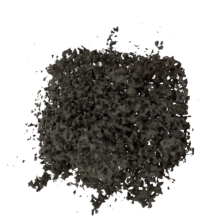
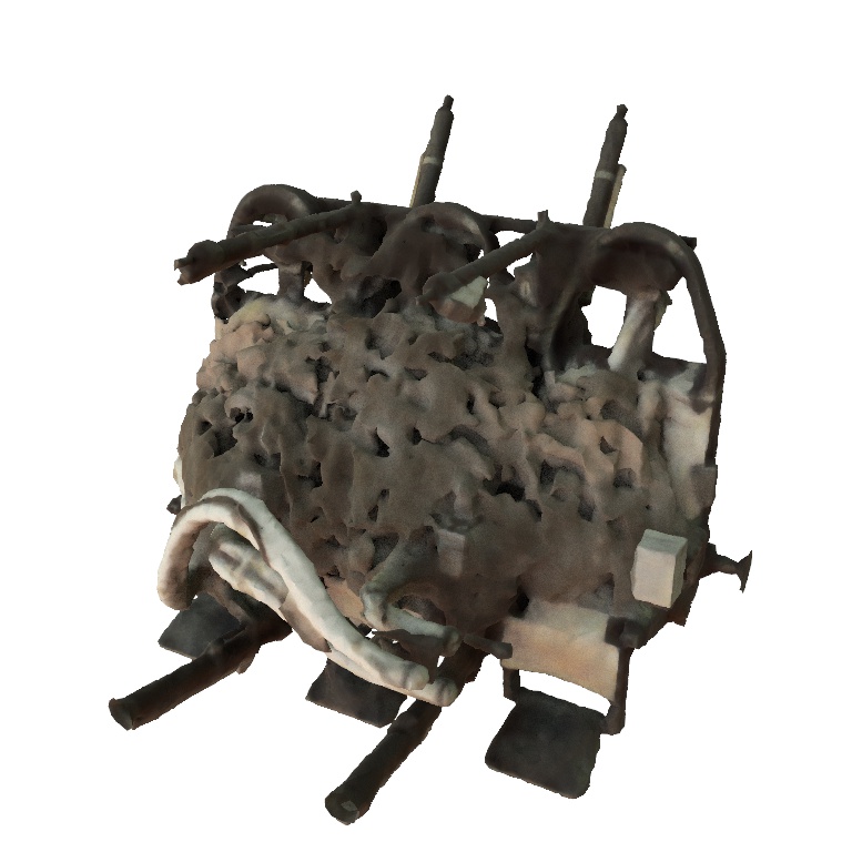
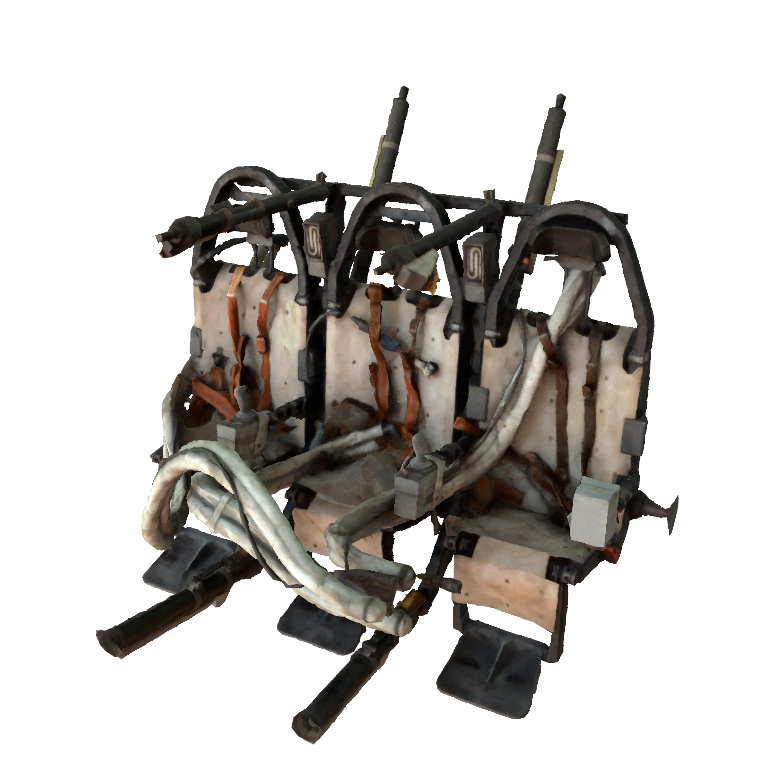
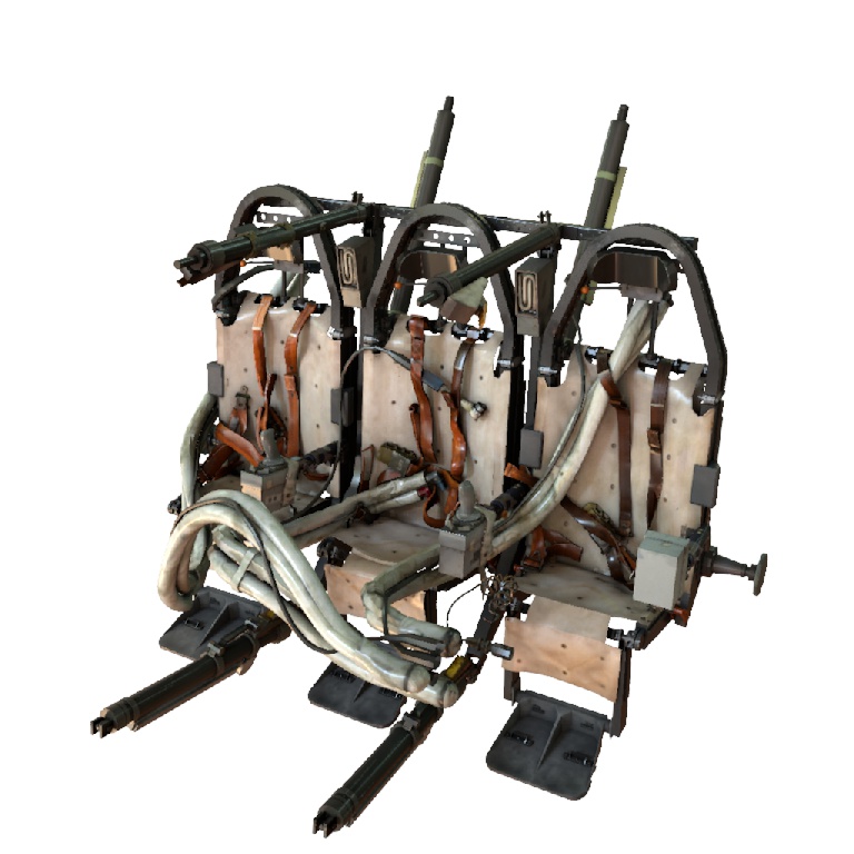
using Adam [26] based on gradients w.r.t. the optimization parameters, , and , which are obtained through differentiable rendering. We use the same loss function as nvdiffrec. An example of the optimization process is illustrated in Figure 3,
 |
 |
 |
 |
 |
 |
| 1 | 10 | 100 | 1000 | 5000 | Reference |
3.1 Direct Illumination
The outgoing radiance in direction can be expressed using the rendering equation [24] as:
| (2) |
This is an integral of the product of the incident radiance, from direction and the BSDF . The integration domain is the hemisphere around the surface normal, .
Spherical Harmonics (SH) [11] or Spherical Gaussians (SG) [6, 73] are often used as efficient approximations of direct illumination, but only work well for low- to medium-frequency lighting. In contrast, the split sum approximation [25, 41] captures all-frequency image based lighting, but does not incorporate shadows. Our goal is all-frequency lighting including shadows, which we tackle by evaluating the rendering equation using Monte Carlo integration:
| (3) |
with samples drawn from some distribution . Note that includes a visibility test, which can be evaluated by tracing a shadow ray in direction . Unfortunately, the variance levels in Monte Carlo integration with low number of samples makes gradient-based optimization hard, particularly with complex lighting. In Section 4 we propose several variance reduction techniques, which enable an inverse rendering pipeline that efficiently reconstructs complex geometry, a wide range of lighting conditions and spatially-varying BSDFs.
Shadow gradients
In single view optimization [60], shape from shadows [57], or direct optimization of the position/direction of analytical light sources, shadow ray visibility gradients [36, 3] are highly beneficial. However, in our multi-view setting (50+ views), similar to Loubet et al. [36], we observed that gradients of diffuse scattering are negligible compared to the gradients of primary visibility. Hence, for performance reasons, in the experiment presented in this paper, the shadow ray visibility gradients are detached when evaluating the hemisphere integral, and shape optimization is driven by primary visibility gradients, obtained from nvdiffrast [28].
4 Variance Reduction
We evaluate direct illumination with high frequency environment map lighting combined with a wide range of materials (diffuse, dielectrics, and metals). Strong directional sunlight, highly specular, mirror-like materials, and the visibility component can all introduce significant levels of noise. To enable optimization in an inverse rendering setting at practical sample counts, we carefully sample each of these contributing factors to obtain a signal with low variance. Below, we describe how we combat noise by using multiple importance sampling and denoising.
4.1 Multiple Importance Sampling
We leverage multiple importance sampling [58] (MIS), a framework to weigh a set of different sampling techniques to reduce variance in Monte Carlo integration. Given a set of sampling techniques, each with a sampling distribution , the Monte Carlo estimator for an integral given by MIS is
| (4) |
The weighting functions are chosen using the balance heuristic. Please refer to Veach’s thesis [58] or the excellent PBRT book [48] for further details.
In our case, we apply MIS with three sampling techniques: light importance sampling, , using a piecewise-constant 2D distribution sampling technique [48], cosine sampling, , for the diffuse lobe, and GGX importance sampling [23], , for the specular lobe. Unlike in forward rendering with known materials and lights, our material and light parameters are optimization variables. Thus, the sampling distributions, , are recomputed in each optimization iteration. Following the taxonomy of differentiable Monte Carlo estimators of Zeltner et al. [71], our importance sampling is detached, i.e., we do not back-propagate gradients to the scene parameters in the sampling step, only in the material evaluation. Please refer to Zeltner et al. for a careful analysis of Monte Carlo estimators for differentiable light transport.
MIS is unbiased, but chaining multiple iterations of our algorithm exhibits bias, as the current, importance sampled, iteration dictates the sampling distributions used in the next iteration. Light probe intensities, for example, are optimized based on an importance sampled image, which are then used to construct the sampling distribution for the subsequent pass. For unbiased rendering, the sampling distribution must be estimated using a second set of uncorrelated samples instead. Furthermore, we explicitly re-use the random seed from the forward pass during gradient backpropagation to scatter gradients to the exact same set of parameters that contributed to the forward rendering. This approach is clearly biased [59], but we empirically note that this is very effective in reducing variance, and in our setting this variance-bias trade-off works in our favor.
4.2 Denoising
For differentiable rendering, the benefits of denoising are twofold. First, it improves the image quality of the rendering in the forward pass, reducing the optimization error and the gradient noise introduced in the image loss. Second, as gradients back-propagate through the denoiser’s spatial filter kernel, gradient sharing between neighboring pixels is enabled. To see this, let’s consider a simple denoiser, , where the noisy rendered image is filtered by a low-pass filter, ( represents an image space 2D convolution). Given a loss gradient, , the gradients propagated back to the renderer are , which applies the same low-pass filter in case the filter is rotationally symmetric (). In other words, the renderer sees filtered loss gradients in a local spatial footprint. While denoisers inherently trade a reduction in variance for increased bias, we empirically note that denoising significantly helps convergence at lower sample counts, and help to reconstruct higher frequency environment lighting. We show an illustrative example in Figure 9.

Following previous work in denoising for production rendering [2], Figure 4 shows how we separate lighting into diffuse, , and specular, terms. This lets us denoise each term separately, creating denoised buffers, , and . More importantly, we can use demodulated diffuse lighting, which means that the lighting term has not yet been multiplied by material diffuse albedo, . In forward rendering, this is important as it decorrelates the noisy lighting from material textures, thus selectively denoising the noisy Monte-Carlo estimates and avoiding to low-pass filter high-frequent texture information. In inverse rendering, we can additionally use it to improve material and light decomposition by adding regularization on the lighting terms, as disucussed in Section 5. We compose the final image as . We currently do not demodulate specular lighting because of the view dependent Fresnel term, but expect this to be improved in future work.

Cross-bilateral filters
Cross-bilateral filters are commonly used to remove noise in rendered images [78]. To evaluate this family of denoisers in our inverse pipeline, we adapted Spatio-temporal Variance-Guided Filtering [52] (SVGF), which is a popular cross-bilateral filter using surface normals and per-pixel depth as edge-stopping guides. The denoiser is applied to demodulated diffuse lighting, to avoid smearing texture detail. We disabled the temporal component of SVGF, as we focus on single frame rendering, and implemented the filter as a differentiable module to allow for loss gradients to propagate back to our scene parameters.
Neural denoisers
As a representative neural denoiser, we deploy the Open Image Denoiser (OIDN) [1], which is a U-Net [51] pre-trained on a large corpus of rendered images. The denoiser is applied to the rendered image before computing the image space loss. As the network model is fully convolutional, it is trivially differentiable, and we can propagate gradients from the image space loss, through the denoiser back to the renderer.
In Figure 5, we provide an overview on the effect of denoisers during 3D scene reconstruction. We observe that denoising is especially helpful at low sample counts, where we obtain similar reconstruction results at 8 spp with denoising, compared to 32 spp without a denoiser. At higher sample counts, however, the benefit from denoising diminishes, as variance in the Monte-Carlo estimates decreases. Given that denoisers enable significantly faster iteration times, we consider it a valuable tool for saving computational resources when fine-tuning model parameters for subsequent runs with high sample counts. Additionally, we empirically found that using a denoiser during reconstruction yields higher quality light probes, as can be seen in Figure 9, both at low and high sample counts.
We can also jointly optimize the denoiser parameters, , with the 3D scene reconstruction task. i.e., the denoiser is fine-tuned for the current scene. Unfortunately, this approach has undesirable side-effects: Features tend to get baked into the denoiser network weights instead of the materials or light probe. This is especially apparent with the OIDN [1] denoiser, which produced color shifts due to lack of regularization on the output. We got notably better results with the hierarchical kernel prediction architecture from Hasselgren et al. [22], which is more constrained. However, the results still lagged behind denoisers with locked weights. We refer to the supplemental material for details.
5 Priors
In our setting: 3D reconstruction from multi-view images with constant lighting, regularization is essential in order to disentangle lighting and materials. Following previous work [75, 41], we apply smoothness priors for albedo, specular, and normal map textures. Taking the albedo as an example, if denotes the diffuse albedo at world space position, , and is a small random displacement vector, we define the smoothness prior for albedo as:
| (5) |
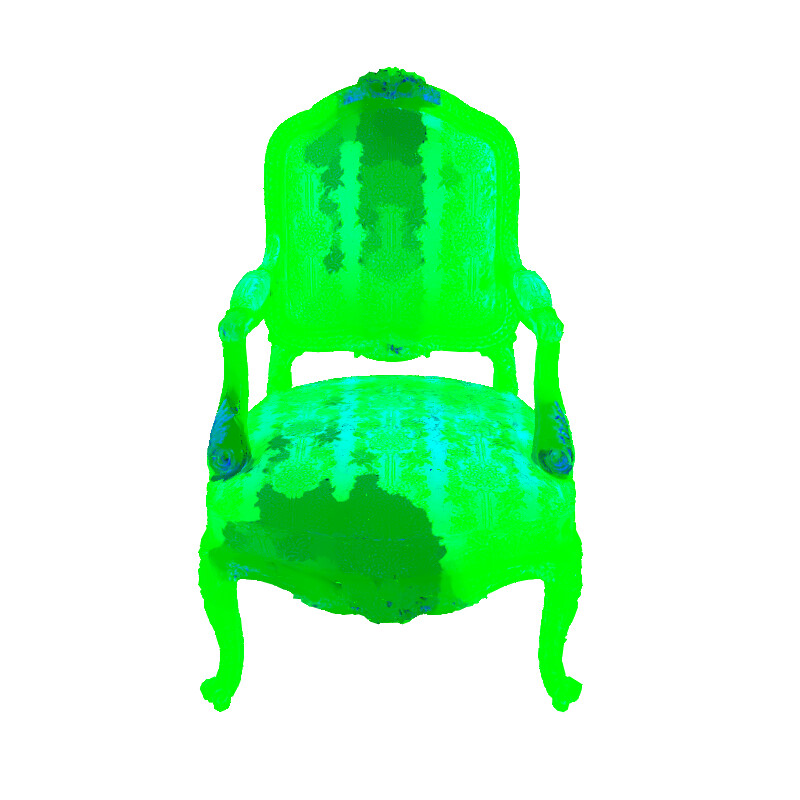
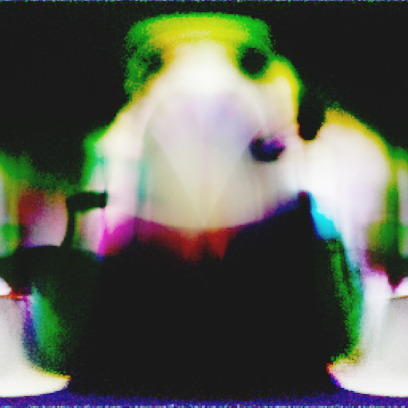
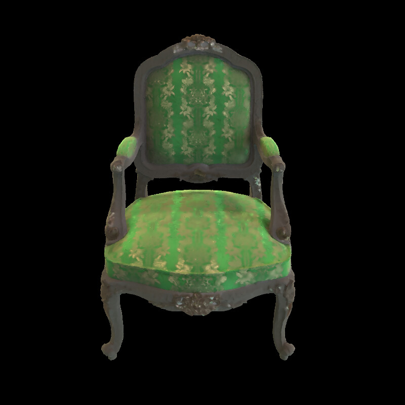
where are the world space positions at the primary hit point on the object. We note that the smoothness prior is not sufficient to disentangle material parameters and light, especially for scenes with high frequency lighting and sharp shadows. Optimization tends to bake shadows into the albedo texture (easy) rather than reconstruct a high intensity, small area in the environment map (hard). To enable high quality relighting, we explicitly want to enforce shading detail represented by lighting, and only bake remaining details into the material textures. We propose a novel regularizer term that is surprisingly effective. We compute a monochrome image loss between the demodulated lighting terms and the reference image:
| (6) |
Here, is a simple luminance operator, and is the HSV value component. The rationale for using HSV-value for the reference image is that the operation approximates demodulation, e.g., a red and white pixel have identical values. We assume that the demodulated lighting is mostly monochrome, in which case , and given that we need to propagate gradients to and , avoids discontinuities. This regularizer is limited by our inability to demodulate the reference image. The HSV-value ignores chrominance, but we cannot separate a shadow from a darker material. This has not been a problem in our tests, but could interfere with optimization if the regularizer is given too much weight. Please refer to the supplemental materials for complete regularizer details.
6 Experiments
| NeRFactor synthetic | Nerf synthetic | Our synthetic | |||||||
|---|---|---|---|---|---|---|---|---|---|
| PSNR | SSIM | LPIPS | PSNR | SSIM | LPIPS | PSNR | SSIM | LPIPS | |
| Our | 26.0 dB | 0.924 | 0.060 | 26.5 dB | 0.932 | 0.055 | 27.1 dB | 0.950 | 0.027 |
| nvdiffrec | 24.8 dB | 0.910 | 0.063 | 23.3 dB | 0.889 | 0.076 | 23.7 dB | 0.925 | 0.049 |
| NeRFactor | 22.2 dB | 0.896 | 0.087 | - | - | - | - | - | - |
|
Ref |
||||||||
|---|---|---|---|---|---|---|---|---|
|
nvdiffrec |
||||||||
|
Our |
||||||||
| Drums | Hotdog | Lego | Ficus | Chair | Hotdog | Lego | Materials | |
| NeRFactor dataset | NeRF synthetic dataset | |||||||
In our experiments, we use nvdiffrec [41] as a baseline, and refer to their work for thorough comparisons against related work. We focus the evaluation on the quality of material and light separation. At test time, all view interpolation results are generated without denoising at 2k spp. All relighting results are rendered in Blender Cycles at 64 spp with denoising [1]. Table 1 shows a quantitative comparison with nvdiffrec and NeRFactor [75] on the NeRFactor relighting setup. Note that there is an indeterminate scale factor between material reflectance (e.g., albedo) and the light intensity. This is accounted for by scaling each image to match the average luminance of the reference for the corresponding scene. The same methodology is applied for all algorithms in our comparisons. We outperform previous work, providing better material reconstruction. Figure 6 shows visual examples.
 |
 |
 |
| Our reconstruction | Material edits | |
 |
 |
 |
| Scene edit | Relighting | |
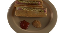
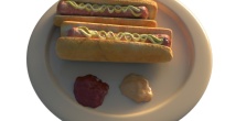
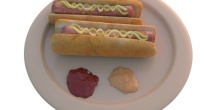
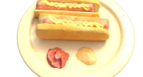
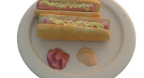
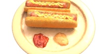
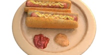
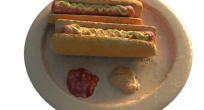
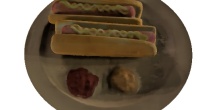
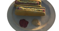
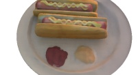
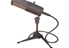
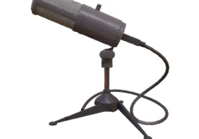
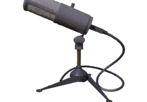
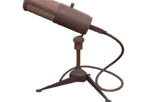
We additionally perform relighting on the synthetic NeRF dataset, which is substantially more challenging than the NeRFactor variant, due to high frequency lighting and global illumination effects. nvdiffrec produces severe artifacts, as exemplified by the Hotdog scene in Figure 6. Table 1 shows a significant increase in image quality for our approach. The visual examples show that our results are plausible, though not without artifacts. Finally, we constructed a novel synthetic dataset with three scenes with highly complex geometry to stress-test the system. Each scene contains 200 training views and 200 novel views for evaluation. The three scenes are shown in Figures 1 , 3 ,and 9. Quantitatively we outperform previous work by a larger margin, and Figure 1 shows very little shading in the albedo textures.
| Family | 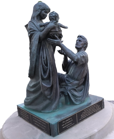 |
 |
Our | |||||
| nvdiffrec | ||||||||
| Character | Our | |||||||
| nvdiffrec | ||||||||
| Gold Cape | 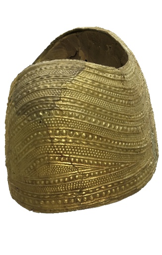 |
 |
Our | |||||
| nvdiffrec | ||||||||
| Ref | Our | Geometry | Normal | Probe |
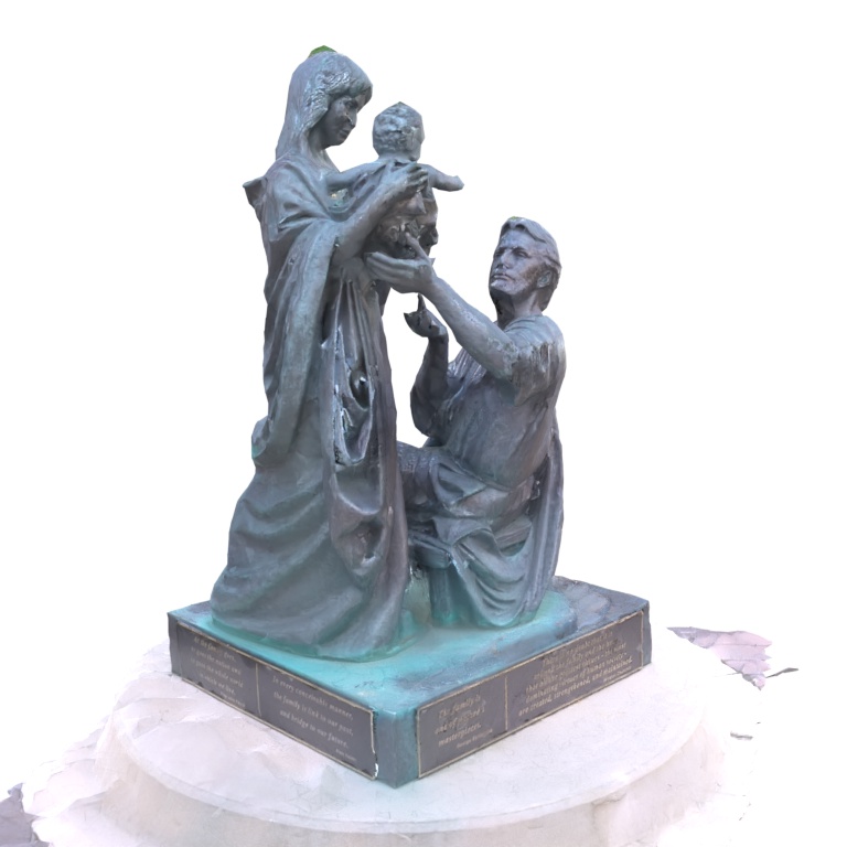
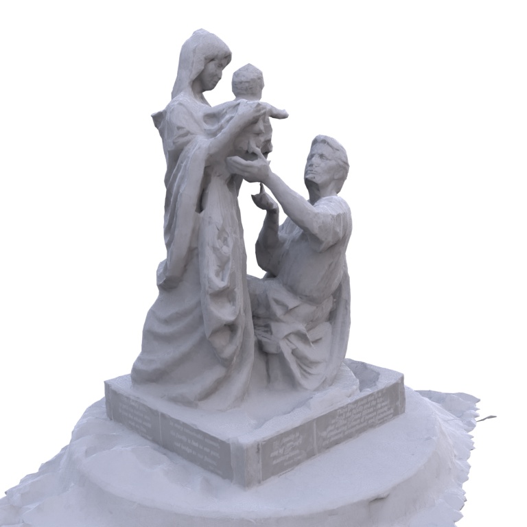
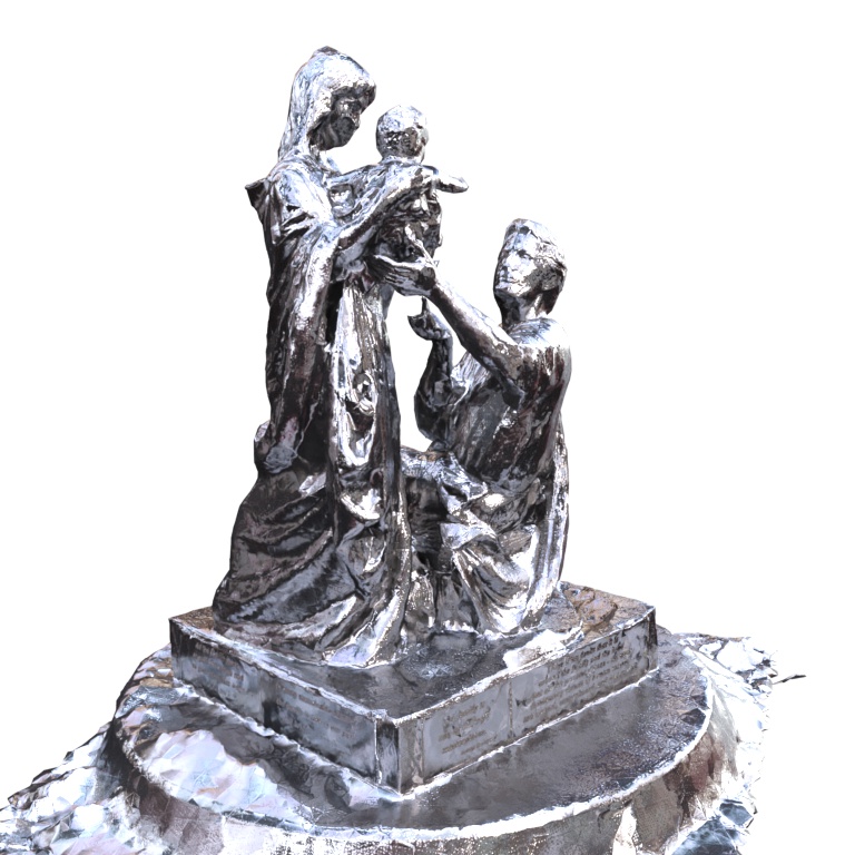
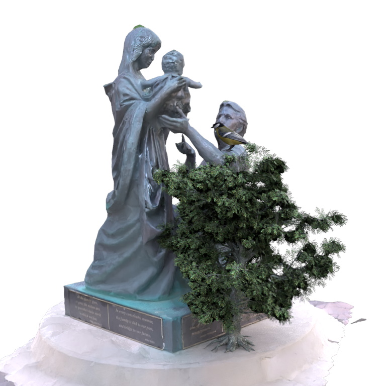
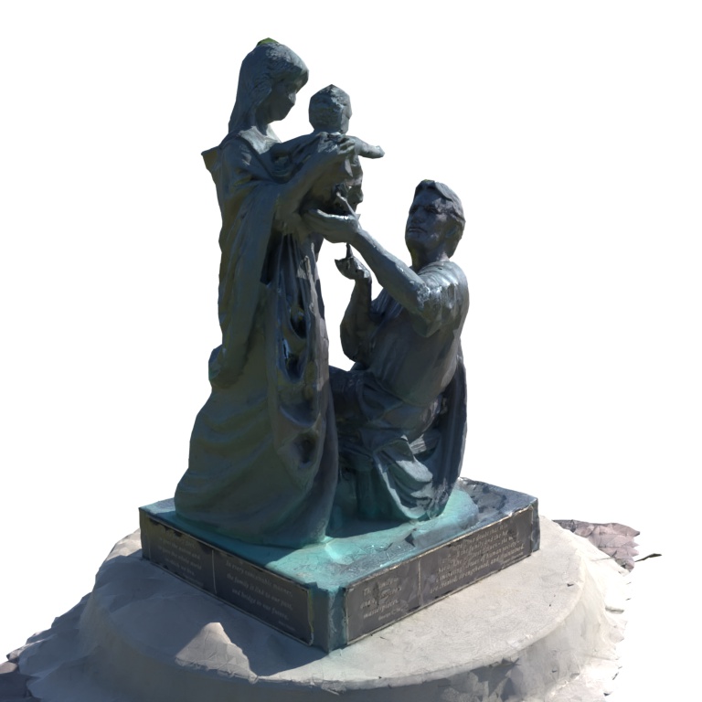
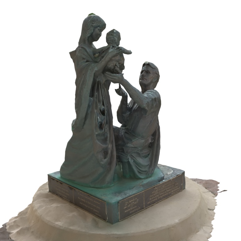
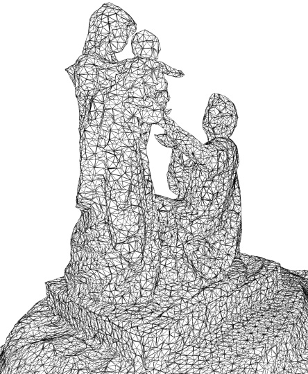
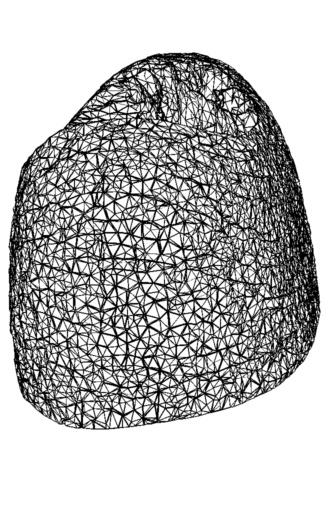
In Figures 7 and 8, we apply our method to datasets with real photos. These sets are more difficult, due to inaccuracies in foreground segmentation masks and camera poses. We extract triangle meshes that can be trivially edited in 3D modeling software, and in Figure 7 we use Blender to perform material editing and relighting with convincing results. Figure 8 shows a breakdown of geometry, material parameters, and environment light.
| PSNR | 24.4 dB | 25.7 dB | 25.6 dB | 26.0 dB | |
| Reference | 8 spp | 8 spp denoised | 128 spp | 128 spp denoised |
To study the impact of denoising, we optimized the Porsche scene w/ and w/o denoising. As shown in Figure 9, denoising improves both visual quality and environment lighting detail at equal sample counts. The noise levels varies throughout the scene, and we note that denoising is particularly helpful in regions with complex lighting or occlusion, such as the specular highlight and cockpit.
| NeRFactor synthetic | Nerf synthetic | Our synthetic | Real-world | |||||
|---|---|---|---|---|---|---|---|---|
| PSNR | SSIM | PSNR | SSIM | PSNR | SSIM | PSNR | SSIM | |
| Our | 29.6 dB | 0.951 | 28.4 dB | 0.938 | 25.6 dB | 0.934 | 25.29 dB | 0.899 |
| nvdiffrec | 31.7 dB | 0.967 | 30.4 dB | 0.958 | 25.8 dB | 0.944 | 26.58 dB | 0.918 |
Neural light-fields, e.g., Mip-NeRF [4] excel at view interpolation. We enforce material/light separation through additional regularization, which slightly degrades view interpolation results, as shown in Table 2. Our scores are slightly below nvdiffrec, but, as shown above, we provide considerably better material and lighting separation.
Compute resources
Tracing rays to evaluate the direct illumination is considerably more expensive than pre-filtered environment light approaches. We leverage hardware-accelerated ray intersections, but note that our implementation is far from fully optimized. Our method scales linearly with sample count, which gives us a simple way to trade quality for performance. With a batch size 8 at a rendering resolution of 512512, we get the following iteration times on a single NVIDIA A6000 GPU.
| nvdiffrec | Our 2 spp | Our 8 spp | Our 32 spp | Our 128 spp | Our 288 spp | |
| Iteration time | 340 ms | 280 ms | 285 ms | 300 ms | 360 ms | 450 ms |
Our denoising strategies enable optimization at low sample counts. Unless otherwise mentioned, for the results presented in the paper, we use high quality settings of 128+ rays per pixel with 50002 iterations (second pass with fixed topology and 2D textures), which takes 4 hours (A6000).
7 Conclusions
Our restriction to direct illumination shows up in scenes with global illumination. Similarly, we do not handle specular chains (geometry seen through a glass window). For this, we need to integrate multi-bounce path tracing, which is a clear avenue for future work, but comes with additional challenges in increased noise-levels, visibility gradients through specular chains, and drastically increased iteration times. Our renderer is intentionally biased to improve optimization times, but unbiased rendering could expect to generate better results for very high sample counts. Other limitations include lack of efficient regularization of material specular parameters and reliance on a foreground segmentation mask. Our approach is computationally intense, requiring a high-end GPU for optimization runs.
To summarize, we have shown that differentiable Monte-Carlo rendering combined with variance-reduction techniques is practical and applicable to multi-view 3D object reconstruction of explicit triangular 3D models. Our physically-based renderer clearly improves material and light reconstruction over previous work. By leveraging hardware accelerated ray-tracing and differentiable image denoisers, we remain competitive to previous work in terms of optimization time.
References
- [1] Attila T. Áfra. Open Image Denoise, 2022. https://www.openimagedenoise.org/.
- [2] Steve Bako, Thijs Vogels, Brian McWilliams, Mark Meyer, Jan Novák, Alex Harvill, Pradeep Sen, Tony DeRose, and Fabrice Rousselle. Kernel-Predicting Convolutional Networks for Denoising Monte Carlo Renderings. ACM Trans. Graph., 36(4):97:1–97:14, 2017.
- [3] Sai Bangaru, Tzu-Mao Li, and Frédo Durand. Unbiased Warped-Area Sampling for Differentiable Rendering. ACM Trans. Graph., 39(6):245:1–245:18, 2020.
- [4] Jonathan T. Barron, Ben Mildenhall, Matthew Tancik, Peter Hedman, Ricardo Martin-Brualla, and Pratul P. Srinivasan. Mip-NeRF: A Multiscale Representation for Anti-Aliasing Neural Radiance Fields. In International Conference on Computer Vision (ICCV), pages 5855–5864, 2021.
- [5] Sai Bi, Zexiang Xu, Pratul Srinivasan, Ben Mildenhall, Kalyan Sunkavalli, Miloš Hašan, Yannick Hold-Geoffroy, David Kriegman, and Ravi Ramamoorthi. Neural Reflectance Fields for Appearance Acquisition. arXiv:2008.03824, 2020.
- [6] Mark Boss, Raphael Braun, Varun Jampani, Jonathan T. Barron, Ce Liu, and Hendrik P.A. Lensch. NeRD: Neural Reflectance Decomposition from Image Collections. In International Conference on Computer Vision (ICCV), pages 5855–5864, 2021.
- [7] Mark Boss, Varun Jampani, Raphael Braun, Ce Liu, Jonathan T. Barron, and Hendrik P.A. Lensch. Neural-PIL: Neural Pre-Integrated Lighting for Reflectance Decomposition. In Advances in Neural Information Processing Systems (NeurIPS), pages 10691–10704, 2021.
- [8] Mark Boss, Varun Jampani, Kihwan Kim, Hendrik Lensch, and Jan Kautz. Two-shot spatially-varying BRDF and shape estimation. In Proc. of the IEEE/CVF Conference on Computer Vision and Pattern Recognition (CVPR), pages 3982–3991, 2020.
- [9] Brent Burley. Physically Based Shading at Disney. In SIGGRAPH Courses: Practical Physically Based Shading in Film and Game Production, 2012.
- [10] Chakravarty R. Alla Chaitanya, Anton S. Kaplanyan, Christoph Schied, Marco Salvi, Aaron Lefohn, Derek Nowrouzezahrai, and Timo Aila. Interactive Reconstruction of Monte Carlo Image Sequences Using a Recurrent Denoising Autoencoder. ACM Trans. Graph., 36(4):98:1–98:12, 2017.
- [11] Wenzheng Chen, Jun Gao, Huan Ling, Edward Smith, Jaakko Lehtinen, Alec Jacobson, and Sanja Fidler. Learning to predict 3d objects with an interpolation-based differentiable renderer. In Advances In Neural Information Processing Systems (NeurIPS), 2019.
- [12] Wenzheng Chen, Joey Litalien, Jun Gao, Zian Wang, Clement Fuji Tsang, Sameh Khalis, Or Litany, and Sanja Fidler. DIB-R++: Learning to Predict Lighting and Material with a Hybrid Differentiable Renderer. In Advances in Neural Information Processing Systems (NeurIPS), pages 22834–22848, 2021.
- [13] Duan Gao, Xiao Li, Yue Dong, Pieter Peers, Kun Xu, and Xin Tong. Deep Inverse Rendering for High-Resolution SVBRDF Estimation from an Arbitrary Number of Images. ACM Trans. Graph., 38(4):134:1–134:15, 2019.
- [14] Jun Gao, Wenzheng Chen, Tommy Xiang, Clement Fuji Tsang, Alec Jacobson, Morgan McGuire, and Sanja Fidler. Learning Deformable Tetrahedral Meshes for 3D Reconstruction. In Advances in Neural Information Processing Systems (NeurIPS), pages 9936–9947, 2020.
- [15] Stephan J Garbin, Marek Kowalski, Matthew Johnson, Jamie Shotton, and Julien Valentin. FastNeRF: High-Fidelity Neural Rendering at 200FPS. arXiv:2103.10380, 2021.
- [16] Andrew Gardner, Chris Tchou, Tim Hawkins, and Paul Debevec. Linear Light Source Reflectometry. ACM Trans. Graph., 22(3):749–758, 2003.
- [17] Abhijeet Ghosh, Tongbo Chen, Pieter Peers, Cyrus A. Wilson, and Paul Debevec. Estimating Specular Roughness and Anisotropy from Second Order Spherical Gradient Illumination. Computer Graphics Forum, 28(4):1161–1170, 2009.
- [18] D. Guarnera, G. C. Guarnera, A. Ghosh, C. Denk, and M. Glencross. BRDF Representation and Acquisition. In Proceedings of the 37th Annual Conference of the European Association for Computer Graphics: State of the Art Reports, pages 625–650, 2016.
- [19] Yu Guo, Cameron Smith, Miloš Hašan, Kalyan Sunkavalli, and Shuang Zhao. MaterialGAN: Reflectance Capture Using a Generative SVBRDF Model. ACM Trans. Graph., 39(6):254:1–254:13, 2020.
- [20] M. Haindl and J. Filip. Visual Texture. Springer-Verlag, 2013.
- [21] Jon Hasselgren, Jacob Munkberg, Jaakko Lehtinen, Miika Aittala, and Samuli Laine. Appearance-driven automatic 3d model simplification. In Eurographics Symposium on Rendering, 2021.
- [22] Jon Hasselgren, Jacob Munkberg, Anjul Patney, Marco Salvi, and Aaron Lefohn. Neural Temporal Adaptive Sampling and Denoising. Computer Graphics Forum, 39(2):147–155, 2020.
- [23] Eric Heitz. Sampling the GGX Distribution of Visible Normals. Journal of Computer Graphics Techniques (JCGT), 7(4):1–13, 2018.
- [24] James T. Kajiya. The rendering equation. In Proceedings of the 13th annual conference on Computer graphics and interactive techniques - SIGGRAPH’86. ACM Press, 1986.
- [25] Brian Karis. Real shading in unreal engine 4. SIGGRAPH 2013 Course: Physically Based Shading in Theory and Practice, 2013.
- [26] Diederik P. Kingma and Jimmy Ba. Adam: A Method for Stochastic Optimization. In Proceedings of the 3rd International Conference for Learning Representations, 2015.
- [27] Arno Knapitsch, Jaesik Park, Qian-Yi Zhou, and Vladlen Koltun. Tanks and temples: Benchmarking large-scale scene reconstruction. ACM Trans. Graph., 36(4):78:1–78:13, 2017.
- [28] Samuli Laine, Janne Hellsten, Tero Karras, Yeongho Seol, Jaakko Lehtinen, and Timo Aila. Modular primitives for high-performance differentiable rendering. ACM Trans. Graph., 39(6):194:1–194:14, 2020.
- [29] Gerald Lasser. LDraw.org, 2022. https://www.ldraw.org/.
- [30] Hendrik P.A. Lensch, Jochen Lang, Asla M. Sa, and Hans-Peter Seidel. Planned sampling of spatially varying BRDFs. Computer Graphics Forum, 22(3):473–482, 2003.
- [31] Tzu-Mao Li, Miika Aittala, Frédo Durand, and Jaakko Lehtinen. Differentiable Monte Carlo Ray Tracing through Edge Sampling. ACM Trans. Graph., 37(6):222:1–222:11, 2018.
- [32] Zhengqin Li, Mohammad Shafiei, Ravi Ramamoorthi, Kalyan Sunkavalli, and Manmohan Chandraker. Inverse rendering for complex indoor scenes: Shape, spatially-varying lighting and svbrdf from a single image. In Proceedings of the IEEE/CVF Conference on Computer Vision and Pattern Recognition, pages 2475–2484, 2020.
- [33] Zhengqin Li, Zexiang Xu, Ravi Ramamoorthi, Kalyan Sunkavalli, and Manmohan Chandraker. Learning to Reconstruct Shape and Spatially-Varying Reflectance from a Single Image. ACM Trans. Graph., 37(6):269:1–269:11, 2018.
- [34] Yiyi Liao, Simon Donné, and Andreas Geiger. Deep Marching Cubes: Learning Explicit Surface Representations. In Conference on Computer Vision and Pattern Recognition (CVPR), pages 2916–2925, 2018.
- [35] Shichen Liu, Tianye Li, Weikai Chen, and Hao Li. Soft Rasterizer: A Differentiable Renderer for Image-based 3D Reasoning. In International Conference on Computer Vision (ICCV), pages 7707–7716, 2019.
- [36] Guillaume Loubet, Nicolas Holzschuch, and Wenzel Jakob. Reparameterizing Discontinuous Integrands for Differentiable Rendering. ACM Trans. Graph., 38(6):228:1–228:14, 2019.
- [37] Fujun Luan, Shuang Zhao, Kavita Bala, and Zhao Dong. Unified Shape and SVBRDF Recovery using Differentiable Monte Carlo Rendering. arXiv:2103.15208, 2021.
- [38] Ricardo Martin-Brualla, Noha Radwan, Mehdi SM Sajjadi, Jonathan T Barron, Alexey Dosovitskiy, and Daniel Duckworth. Nerf in the wild: Neural radiance fields for unconstrained photo collections. In Proceedings of the IEEE/CVF Conference on Computer Vision and Pattern Recognition, pages 7210–7219, 2021.
- [39] Ben Mildenhall, Pratul P. Srinivasan, Matthew Tancik, Jonathan T. Barron, Ravi Ramamoorthi, and Ren Ng. NeRF: Representing Scenes as Neural Radiance Fields for View Synthesis. In ECCV, 2020.
- [40] Thomas Müller, Alex Evans, Christoph Schied, and Alexander Keller. Instant neural graphics primitives with a multiresolution hash encoding. ACM Trans. Graph., 41(4):102:1–102:15, 2022.
- [41] Jacob Munkberg, Jon Hasselgren, Tianchang Shen, Jun Gao, Wenzheng Chen, Alex Evans, Thomas Mueller, and Sanja Fidler. Extracting Triangular 3D Models, Materials, and Lighting From Images. In 2022 IEEE/CVF Conference on Computer Vision and Pattern Recognition (CVPR), pages 8270–8280, 2022.
- [42] Michael Niemeyer and Andreas Geiger. Giraffe: Representing scenes as compositional generative neural feature fields. In Proceedings of the IEEE/CVF Conference on Computer Vision and Pattern Recognition, pages 11453–11464, 2021.
- [43] Michael Niemeyer, Lars Mescheder, Michael Oechsle, and Andreas Geiger. Differentiable volumetric rendering: Learning implicit 3d representations without 3d supervision. In Proceedings IEEE Conf. on Computer Vision and Pattern Recognition (CVPR), 2020.
- [44] Merlin Nimier-David, Zhao Dong, Wenzel Jakob, and Anton Kaplanyan. Material and Lighting Reconstruction for Complex Indoor Scenes with Texture-space Differentiable Rendering. In Eurographics Symposium on Rendering – DL-only Track, 2021.
- [45] Merlin Nimier-David, Sébastien Speierer, Benoît Ruiz, and Wenzel Jakob. Radiative Backpropagation: An Adjoint Method for Lightning-Fast Differentiable Rendering. ACM Trans. Graph., 39(4):146:1–146:15, 2020.
- [46] Merlin Nimier-David, Delio Vicini, Tizian Zeltner, and Wenzel Jakob. Mitsuba 2: A retargetable forward and inverse renderer. ACM Trans. Graph., 38(6):203:1–203:17, 2019.
- [47] Michael Oechsle, Songyou Peng, and Andreas Geiger. UNISURF: Unifying Neural Implicit Surfaces and Radiance Fields for Multi-View Reconstruction. In International Conference on Computer Vision (ICCV), pages 5589–5599, 2021.
- [48] Matt Pharr and Greg Humphreys. Physically Based Rendering, Second Edition: From Theory To Implementation. Morgan Kaufmann Publishers Inc., 2nd edition, 2010.
- [49] Albert Pumarola, Enric Corona, Gerard Pons-Moll, and Francesc Moreno-Noguer. D-nerf: Neural radiance fields for dynamic scenes. In Proceedings of the IEEE/CVF Conference on Computer Vision and Pattern Recognition, pages 10318–10327, 2021.
- [50] Christian Reiser, Songyou Peng, Yiyi Liao, and Andreas Geiger. KiloNeRF: Speeding up Neural Radiance Fields with Thousands of Tiny MLPs. arXiv:2103.13744, 2021.
- [51] Olaf Ronneberger, Philipp Fischer, and Thomas Brox. U-Net: Convolutional Networks for Biomedical Image Segmentation. In Medical Image Computing and Computer-Assisted Intervention – MICCAI 2015, pages 234–241, 2015.
- [52] Christoph Schied, Anton Kaplanyan, Chris Wyman, Anjul Patney, Chakravarty R. Alla Chaitanya, John Burgess, Shiqiu Liu, Carsten Dachsbacher, Aaron Lefohn, and Marco Salvi. Spatiotemporal Variance-guided Filtering: Real-time Reconstruction for Path-traced Global Illumination. In Proceedings of High Performance Graphics, pages 2:1–2:12, 2017.
- [53] Carolin Schmitt, Simon Donne, Gernot Riegler, Vladlen Koltun, and Andreas Geiger. On Joint Estimation of Pose, Geometry and svBRDF from a Handheld Scanner. In Proc. of the IEEE/CVF Conference on Computer Vision and Pattern Recognition (CVPR), 2020.
- [54] Tianchang Shen, Jun Gao, Kangxue Yin, Ming-Yu Liu, and Sanja Fidler. Deep Marching Tetrahedra: a Hybrid Representation for High-Resolution 3D Shape Synthesis. In Advances in Neural Information Processing Systems (NeurIPS), pages 6087–6101, 2021.
- [55] Smithsonian. Smithsonian 3D Digitization, 2018. https://3d.si.edu/.
- [56] Michael Stokes, Matthew Anderson, Srinivasan Chandrasekar, and Ricardo Motta. A Standard Default Color Space for the Internet - sRGB, 1996.
- [57] Kushagra Tiwary, Tzofi Klinghoffer, and Ramesh Raskar. Towards learning neural representations from shadows. arXiv:2203.15946, 2022.
- [58] Eric Veach and Leonidas J. Guibas. Optimally Combining Sampling Techniques for Monte Carlo Rendering. In Proceedings of the 22nd Annual Conference on Computer Graphics and Interactive Techniques, page 419–428, 1995.
- [59] Delio Vicini, Sébastien Speierer, and Wenzel Jakob. Path replay backpropagation: differentiating light paths using constant memory and linear time. ACM Trans. Graph., 40(4):108:1–108:14, 2021.
- [60] Delio Vicini, Sébastien Speierer, and Wenzel Jakob. Differentiable Signed Distance Function Rendering. ACM Trans. Graph., 41(4):125:1–125:18, 2022.
- [61] Bruce Walter, Stephen R. Marschner, Hongsong Li, and Kenneth E. Torrance. Microfacet Models for Refraction through Rough Surfaces. In Proceedings of the 18th Eurographics Conference on Rendering Techniques, page 195–206, 2007.
- [62] Peng Wang, Lingjie Liu, Yuan Liu, Christian Theobalt, Taku Komura, and Wenping Wang. Neus: Learning neural implicit surfaces by volume rendering for multi-view reconstruction. In Advances in Neural Information Processing Systems (NeurIPS), pages 27171–27183, 2021.
- [63] Zian Wang, Jonah Philion, Sanja Fidler, and Jan Kautz. Learning indoor inverse rendering with 3d spatially-varying lighting. In Proceedings of International Conference on Computer Vision (ICCV), 2021.
- [64] Zirui Wang, Shangzhe Wu, Weidi Xie, Min Chen, and Victor Adrian Prisacariu. NeRF: Neural radiance fields without known camera parameters. arXiv:2102.07064, 2021.
- [65] Michael Weinmann and Reinhard Klein. Advances in Geometry and Reflectance Acquisition (Course Notes). In SIGGRAPH Asia 2015 Courses, 2015.
- [66] Suttisak Wizadwongsa, Pakkapon Phongthawee, Jiraphon Yenphraphai, and Supasorn Suwajanakorn. NeX: Real-time View Synthesis with Neural Basis Expansion. In IEEE Conference on Computer Vision and Pattern Recognition (CVPR), pages 8534–8543, 2021.
- [67] Yao Yao, Zixin Luo, Shiwei Li, Jingyang Zhang, Yufan Ren, Lei Zhou, Tian Fang, and Long Quan. BlendedMVS: A Large-scale Dataset for Generalized Multi-view Stereo Networks. Computer Vision and Pattern Recognition (CVPR), 2020.
- [68] Lior Yariv, Yoni Kasten, Dror Moran, Meirav Galun, Matan Atzmon, Basri Ronen, and Yaron Lipman. Multiview neural surface reconstruction by disentangling geometry and appearance. Advances in Neural Information Processing Systems, 33, 2020.
- [69] Alex Yu, Ruilong Li, Matthew Tancik, Hao Li, Ren Ng, and Angjoo Kanazawa. PlenOctrees for Real-time Rendering of Neural Radiance Fields. In International Conference on Computer Vision (ICCV), pages 5752–5761, 2021.
- [70] Greg Zaal. polyhaven, 2021. https://polyhaven.com/hdris.
- [71] Tizian Zeltner, Sébastien Speierer, Iliyan Georgiev, and Wenzel Jakob. Monte Carlo Estimators for Differential Light Transport. ACM Trans. Graph., 40(4):78:1–78:16, 2021.
- [72] Cheng Zhang, Bailey Miller, Kai Yan, Ioannis Gkioulekas, and Shuang Zhao. Path-Space Differentiable Rendering. ACM Trans. Graph., 39(4):143:1–143:19, 2020.
- [73] Kai Zhang, Fujun Luan, Qianqian Wang, Kavita Bala, and Noah Snavely. PhySG: Inverse Rendering with Spherical Gaussians for Physics-based Material Editing and Relighting. In The IEEE/CVF Conference on Computer Vision and Pattern Recognition (CVPR), 2021.
- [74] Kai Zhang, Gernot Riegler, Noah Snavely, and Vladlen Koltun. Nerf++: Analyzing and improving neural radiance fields. arXiv:2010.07492, 2020.
- [75] Xiuming Zhang, Pratul P. Srinivasan, Boyang Deng, Paul Debevec, William T. Freeman, and Jonathan T. Barron. NeRFactor: Neural Factorization of Shape and Reflectance under an Unknown Illumination. ACM Trans. Graph., 40(6):237:1–237:18, 2021.
- [76] Yuxuan Zhang, Wenzheng Chen, Huan Ling, Jun Gao, Yinan Zhang, Antonio Torralba, and Sanja Fidler. Image GANs meet Differentiable Rendering for Inverse Graphics and Interpretable 3D Neural Rendering. In International Conference on Learning Representations, 2021.
- [77] Yuanqing Zhang, Jiaming Sun, Xingyi He, Huan Fu, Rongfei Jia, and Xiaowei Zhou. Modeling Indirect Illumination for Inverse Rendering. arXiv:2204.06837, 2022.
- [78] Matthias Zwicker, Wojciech Jarosz, Jaakko Lehtinen, Bochang Moon, Ravi Ramamoorthi, Fabrice Rousselle, Pradeep Sen, Cyril Soler, and Sung-Eui Yoon. Recent Advances in Adaptive Sampling and Reconstruction for Monte Carlo Rendering. Computer Graphics Forum, 34(2):667–681, 2015.
Appendix A Optimization and Regularization
Image Loss
Our renderer uses physically-based shading and produces images with high dynamic range. Therefore, the objective function must be robust to the full range of floating-point values. Following recent work in differentiable rendering [21, 41], our image space loss, , computes the norm on tonemapped colors. As tone map operator, , we transform linear radiance values, , according to , where is the sRGB transfer function [56]:
| (7) | |||||
Regularizers
While it is desirable to minimize regularization, in our setting with multi-view images with constant lighting, we have to rely on several priors to guide optimization towards a result with a good separation of geometry, materials, and lighting. As mentioned in the paper, we rely on smoothness regularizers for albedo, , specular parameters, and geometric surface normal, , following:
| (8) |
where is a world space position on the surface of the object and is a small random displacement vector. Regularizing the geometric surface normal (before normal map perturbation) is novel compared to nvdiffrec and helps enforce smoother geometry, particularly in early training.
We note that normal mapping (surface normals perturbed through a texture lookup) also benefits from regularization. While normal mapping is a powerful tool for simulating local micro-geometry, the decorrelation of the geometry and surface normal can be problematic. In some optimization runs, we observe that with normal mapping enabled, the environment light is (incorrectly) leveraged as a color dictionary, where the normal perturbation re-orients the normals of a geometric element to look up a desired color. To prevent this behavior, we use the following regularizer. Given a normal perturbation in tangent space, our loss is defined as
| (9) |
Intuitively, we enforce that normal perturbations, modeling micro-geometry, randomly selected in a small local area, have an expected value of the unperturbed tangent space surface normal, .
|
w/o light reg. |
 |
 |
 |
 |
|---|---|---|---|---|
|
w/ light reg. |
 |
 |
 |
 |
| Shaded | Diffuse Light | Probe |
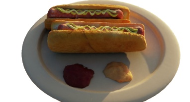
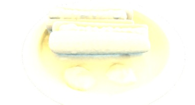
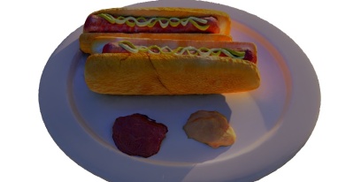
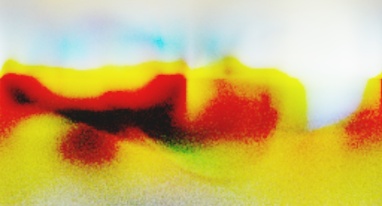
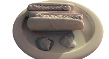
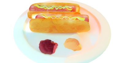
As mentioned in the paper, we additionally regularize based on monochrome image loss between the demodulated lighting terms and the reference image:
| (10) |
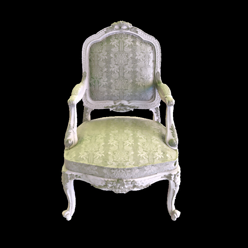
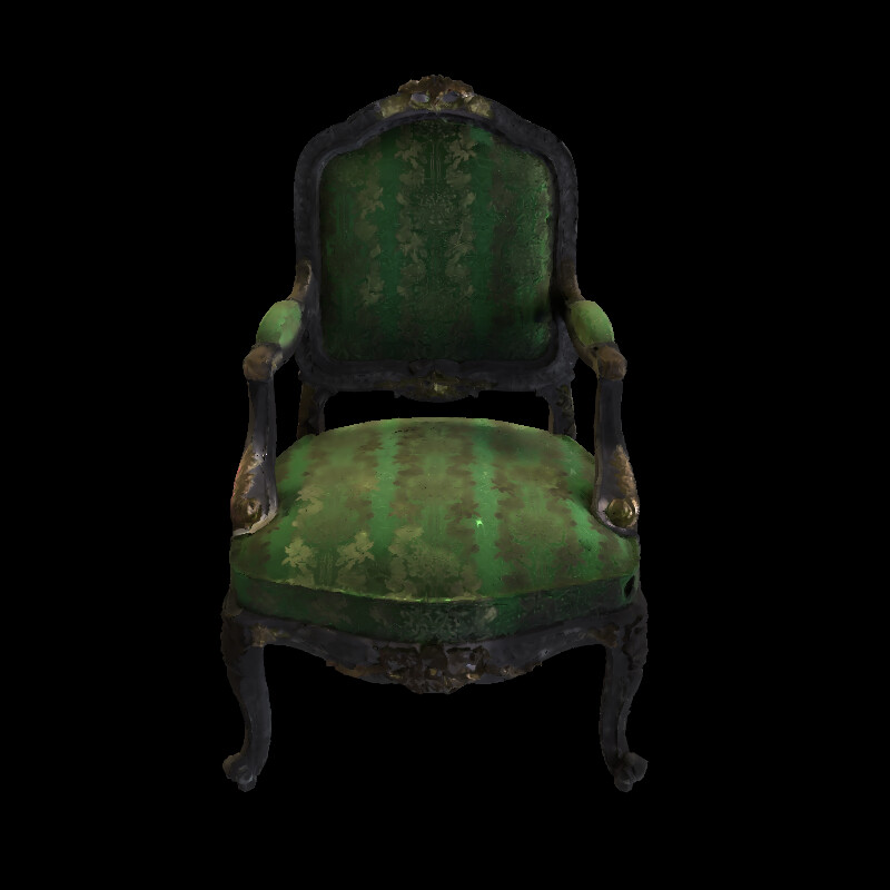
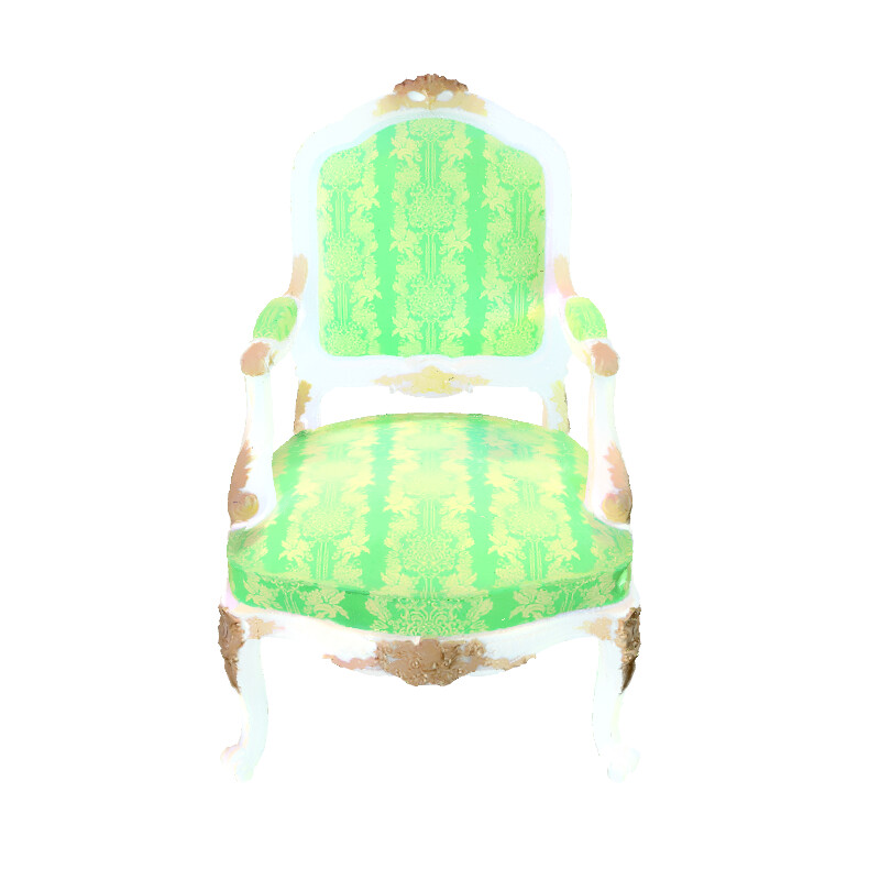
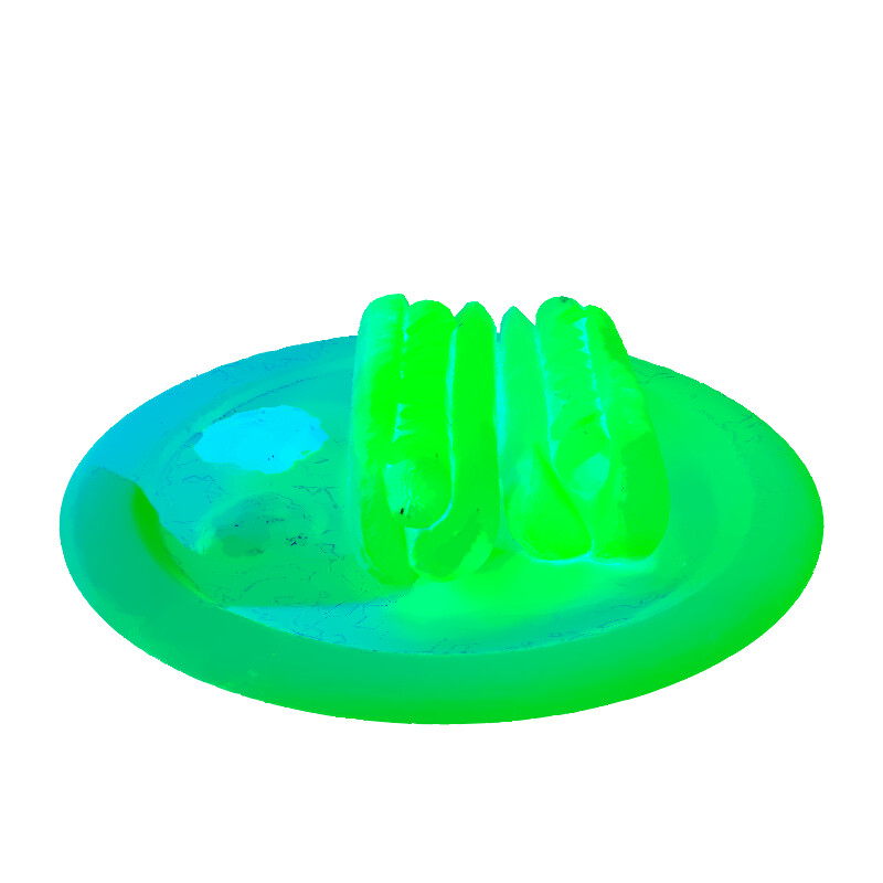
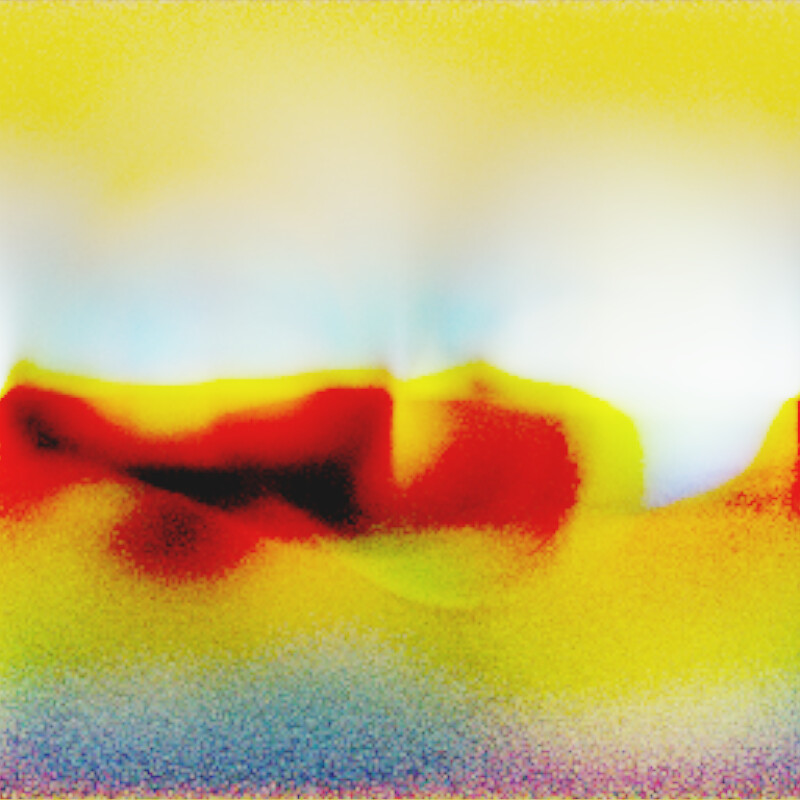
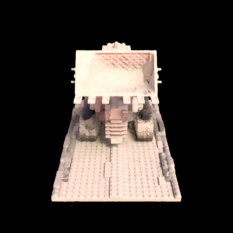
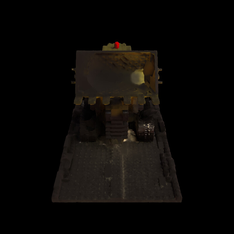
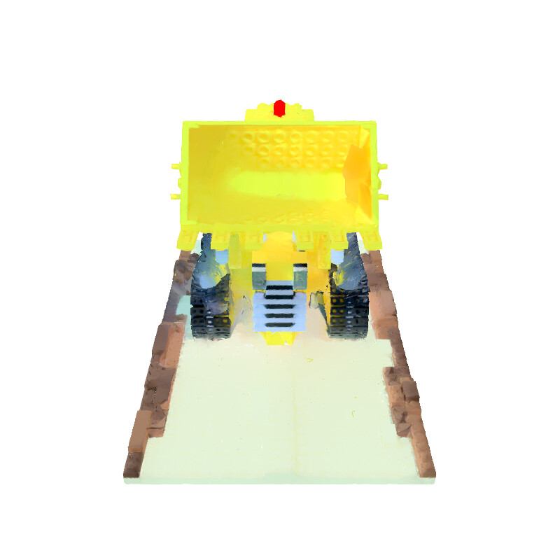
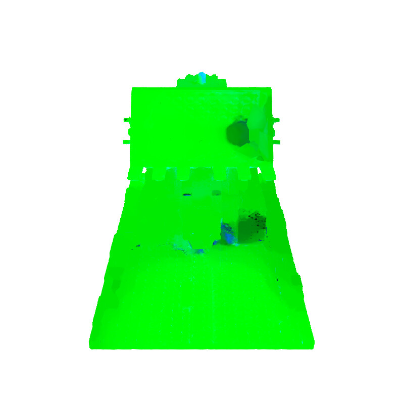
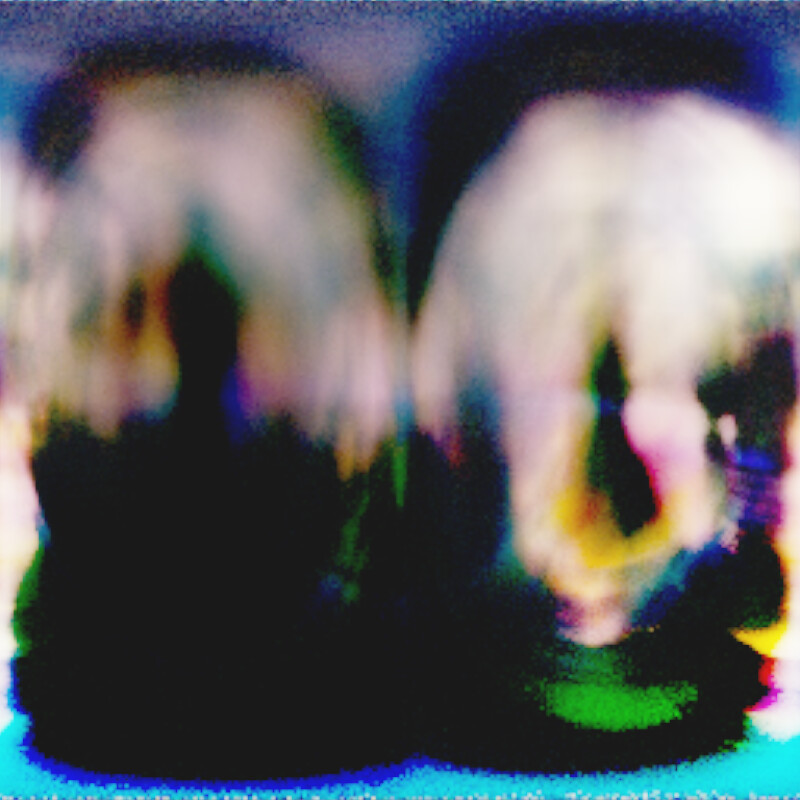
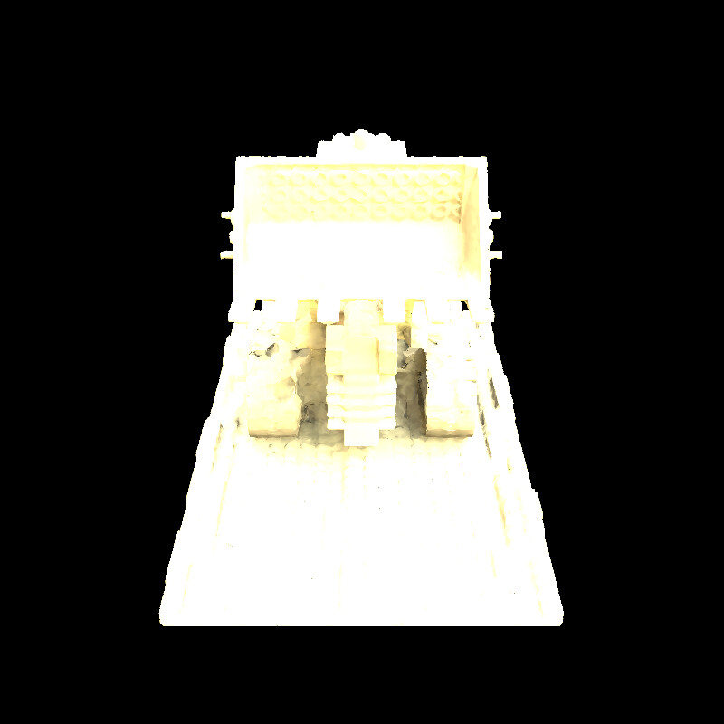
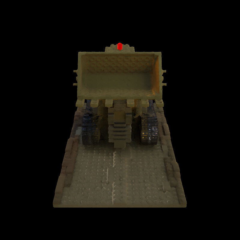
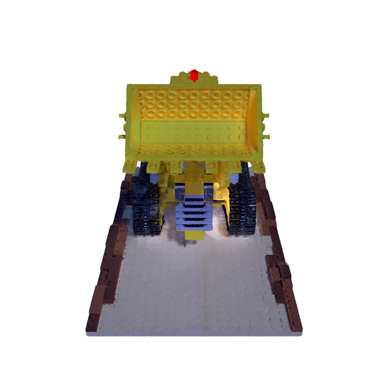
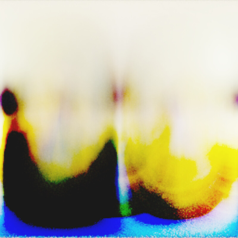
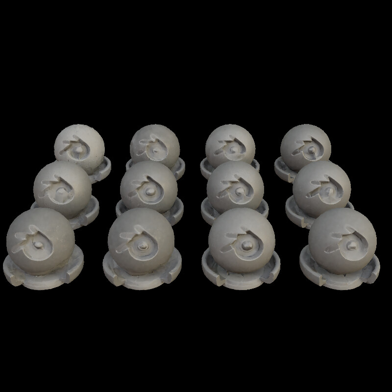
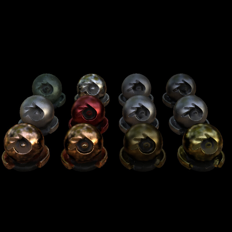
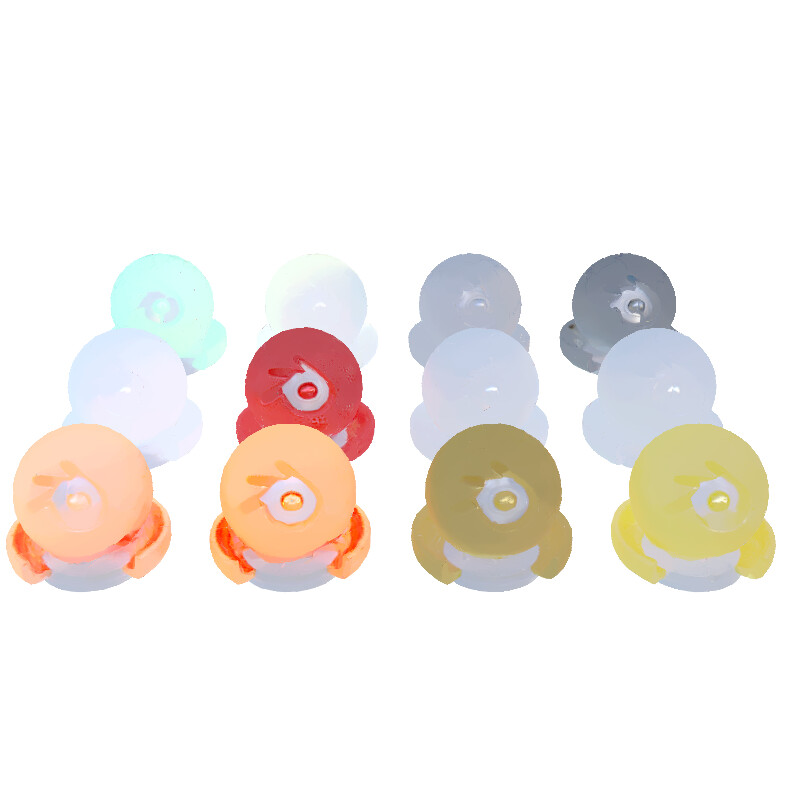
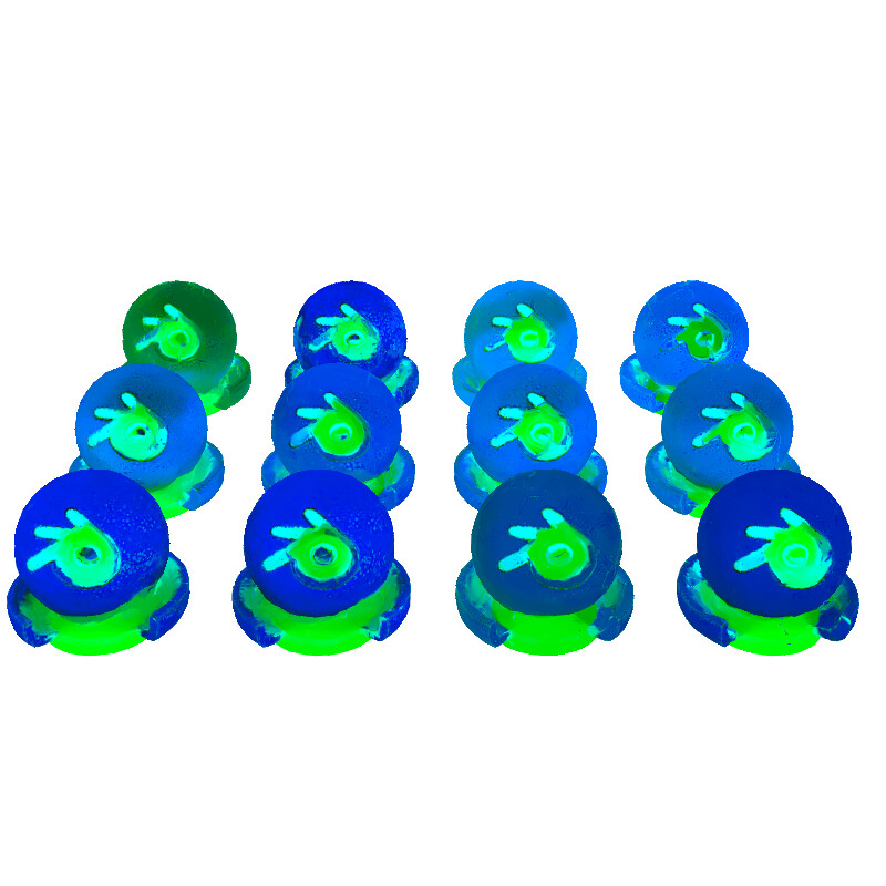
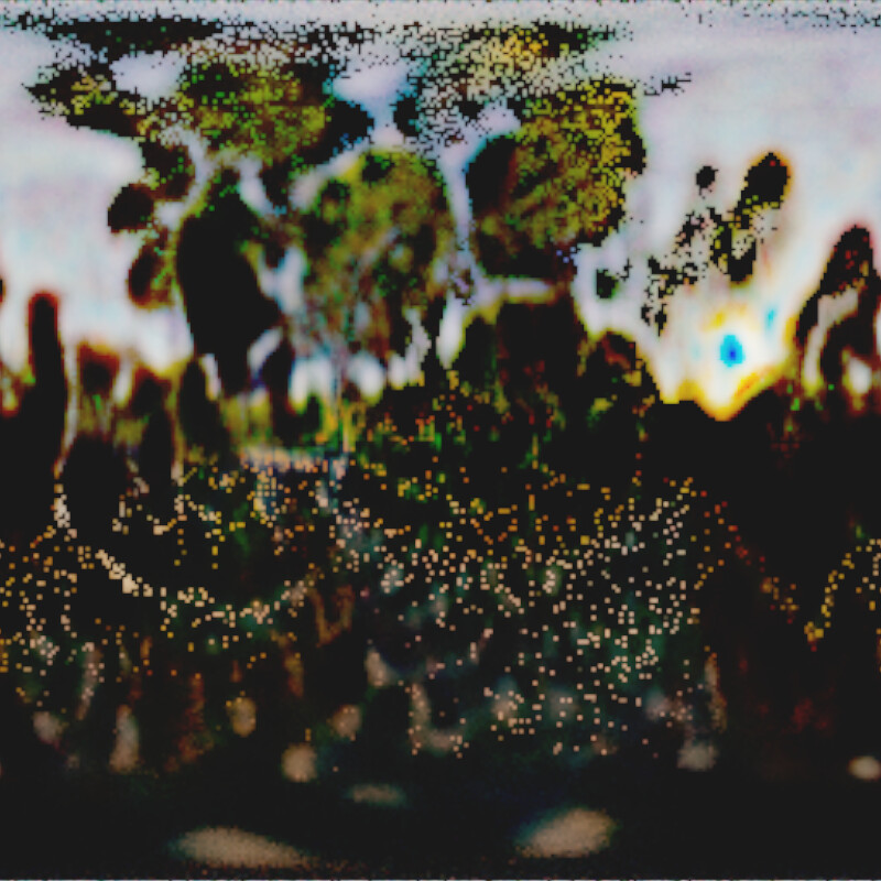
Here, is the tonemap operator described in the previous paragraph. is demodulated diffuse lighting, is specular lighting, and is the target reference image. Monochrome images are computed through the simple luminance operator, , and HSV-value, . While the regularizer is limited by our inability to demodulate the reference image, we show in Figure 10 that it greatly increases lighting detail, which is particularly effective in datasets with high frequency lighting. Figure 27 shows the impact of the regularizer on a larger set of scenes.
We compute the final loss as a weighted combination of the image loss and regularizer terms:
| (11) |
where we show the default weights used for most results (unless otherwise noted).
Optimization details
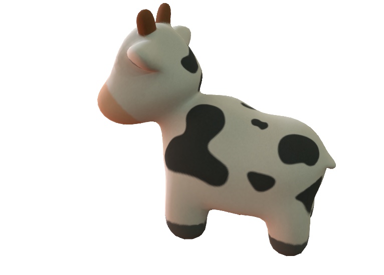
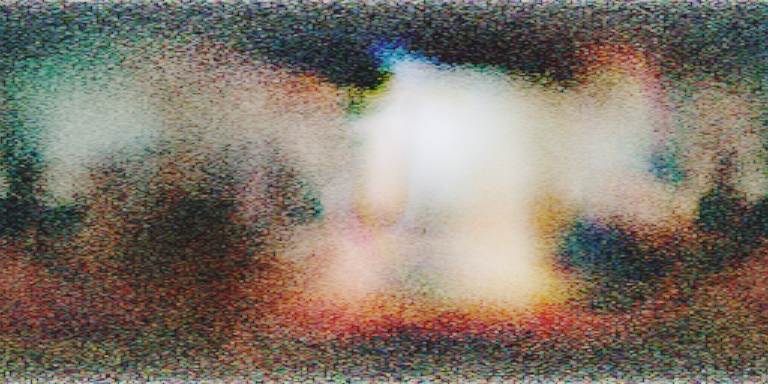
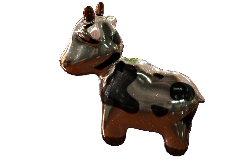
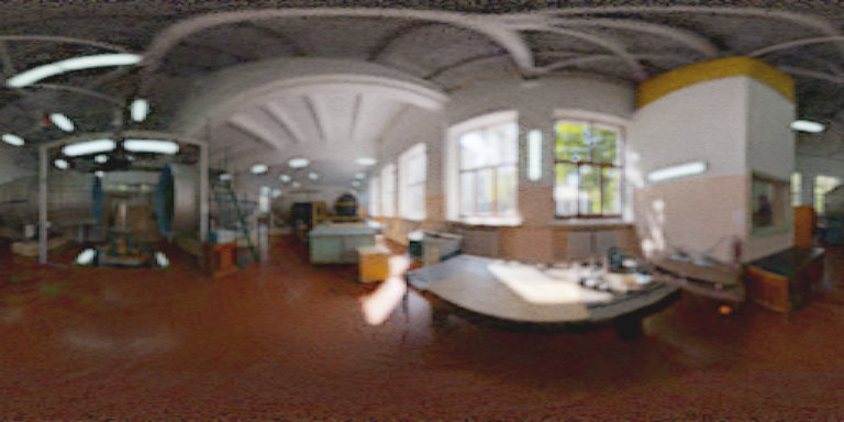
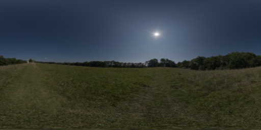
We use Adam [26] (default settings) to optimize parameters for geometry, material, and lighting. Referring to DMTet [54], geometry is parameterized as SDF values on a three-dimensional grid, with a perturbation vector per grid-vertex. Material and lighting are encoded in textures, or neural network (e.g., an MLP with positional encoding) encoded high-frequency functions. We typically use different learning rates for geometry, material, and lighting, with lighting having the highest learning rate and material the lowest. We closely follow the publically available nvdiffrec code base and refer to that for details. In Figure 11, we visualize two examples of optimizing the light probe, and note that we can capture high-frequency lighting details for specular objects.
 |
 |
 |
 |
| Diffuse | Specular | ||
We note that the early phases of optimization (starting from random geometry with large topology changes) are crucial in producing a good final result. The shadow test poses a challenge since changes in geometry may drastically change the lighting intensity in a previously shadowed area, causing the optimization process to get stuck in bad local minima. This is shown in Figure 12, where the optimizer fails to carve out the shape of the object. We combat this by incrementally blending in the shadow term as optimization progresses.
Recall from the main paper that we compute the color according to the rendering equation:
| (12) |
where can be separated into a lighting term, , and visibility term, . Rather than using binary visibility, we introduce a light leakage term, , and linearly fade in the shadow contributions over the first 1750 iterations:
| (13) |
|
w/o blend |
 |
 |
 |
 |
|---|---|---|---|---|
|
w/ blend |
 |
 |
 |
 |
| Shaded | Normals | Shaded | Normals | |
| 500 iterations | 1000 iterations | |||
In Figure 12 we note that gradually blending in the shadow term has a large impact on early convergence. In particular, since we start from a random topology, carving out empty space or adding geometry may have a large impact on overall shading, causing spiky and noisy gradients.
The denoiser may also interfere with early topology optimization (blurred visibility gradients). This is particularly prominent when the denoiser parameters are trained along with scene parameters. Therefore, we similarly, ramp up the spatial footprint, , in the case of a bilateral denoiser. For neural denoisers, which have no easily configurable filter width, we instead linearly blend between the noisy and denoised images to create a smooth progression.
Appendix B Denoising
Bilateral Denoiser
As a representative bilateral denoiser, we adapt the spatial component of Spatiotemporal Variance-guided Filtering [52] (SVGF), Our filter is given by
| (14) |
where are the pixel colors, are the bilateral weights between pixels and , and denotes the filter footprint. The bilateral weight is split into three components as follows
| (15) |
The spatial component, , is a Gaussian filter with its footprint controlled by . We linearly increase from 1e-4 to 2.0 over the first 1750 iterations. The depth component, implements an edge stopping filter based on image space depth. It is a soft test, comparing the depth differences between pixels and with a linear prediction based on the local depth gradient . The final component, , is computed as the scalar product over surface normals and . Following SVGF, we use and . We also omitted the Á-Trous wavelet filtering of SVGF, which is primarily a run-time performance optimization, and evaluate the filter densely in the local footprint. We propagate gradients back to the renderer, i.e., the noisy input colors, but no gradients to the filter weights.

 |
 |
 |
 |
 |
| Reference | No denoising | Bilateral | OIDN (pre-trained) | KPN (live-trained) |
| 8 spp | 26.24 | 36.15 | 35.94 | 35.21 |
| 18 spp | 33.98 | 35.86 | 35.74 | 35.36 |
| 32 spp | 35.87 | 35.72 | 35.65 | 35.19 |
| 128 spp | 36.08 | 35.43 | 35.51 | 35.21 |
| Reference | No denoising | Bilateral | OIDN (pre-trained) | KPN (live-trained) |
| 8 spp | 11.50 | 28.43 | 17.31 | 23.84 |
| 18 spp | 22.12 | 30.99 | 28.85 | 29.07 |
| 32 spp | 25.93 | 30.71 | 30.46 | 27.36 |
| 128 spp | 30.44 | 30.95 | 30.76 | 27.76 |
Neural denoisers
For OIDN, we use the pre-trained weights from the official code [1], and wrap the model (a direct-prediction U-Net) in a PyTorch module to allow for gradient propagation to the input colors. We also propagate gradients to the network weights, in order to fine-tune the denoiser per-scene, but unfortunately, the direct-prediction architecture of OIDN made live-training highly unstable in our setting.
For the kernel-predicting neural denoiser, we leverage the architecture from Hasselgren et al. [22], but omit the adaptive sampling part and the recurrent feedback loop. The network weights were initialized to random values using Xavier initialization. The hierarchical kernel prediction in this architecture constrains the denoiser, and enables live-trained neural denoising in our setting. That said, in our evaluations, the live-trained variant produce worse reconstructions than the pre-trained denoisers.
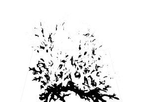
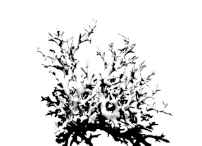
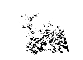
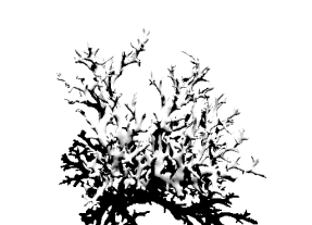
We study the impact of different denoising algorithms on scene reconstruction, including jointly optimizing the denoising network, in Figure 13. Unfortunately, when fine-tuning the denoiser to the specific scene as part of optimization, we note a tendency for features to get baked into the denoiser’s network weights instead of the desired scene parameters (overfitting), negatively impacting the reconstruction quality. We showcase the isolated effect of denoising on light probe optimization in Figure 14. Figure 15 illustrates the effect of denoising when jointly optimizing geometry, material and lighting.
|
Ref |
 |
 |
 |
 |
|---|---|---|---|---|
|
w/o gradients |
 |
 |
 |
 |
|
w/ gradients |
 |
 |
 |
 |
| White | Lambert | Single-view | Multi-view | |
| Light position optimization | Shape optimization | |||
 |
 |
 |
 |
| PSNR — SSIM: 28.21 — 0.945 | PSNR — SSIM: 27.82 — 0.941 |
| w/o shadow gradients | w/ shadow gradients |
Appendix C Visibility Gradients from Shadows
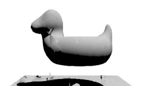
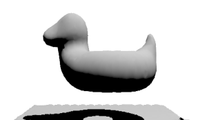
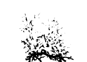
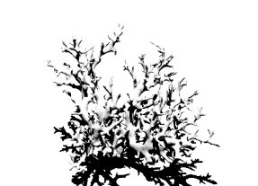
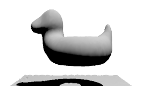
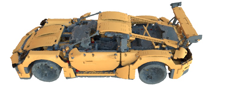
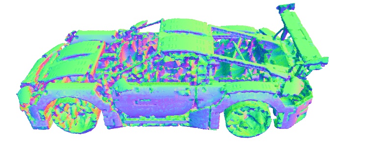
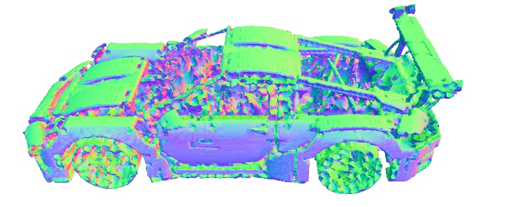
In Figure 16 we show the impact of the visibility gradients [36, 3] for the shadow test on a few targeted reconstruction examples. In this ablation, we disabled denoising, and applied a full shadow term directly (instead of linearly ramping up the shadow contribution, as discussed in Section A). While clearly beneficial in the simpler examples, e.g., single-view reconstruction and targeted optimization (finding the light position), for multi-view reconstruction with joint shape, material, and environment light optimization, the benefits of the shadow visibility gradients is less clear. In our experiments, gradients from the shadow rays in the evaluation of direct lighting in the hemisphere, typically have negligible impact compared to gradients from primary visibility. Below, we report the view-interpolation scores over the validation sets for three scenes.
| PSNR | SSIM | |||||
|---|---|---|---|---|---|---|
| Chair | Lego | Porsche | Chair | Lego | Porsche | |
| w/ gradients | 29.15 | 27.03 | 27.83 | 0.948 | 0.918 | 0.941 |
| w/o gradients | 29.06 | 26.83 | 28.21 | 0.948 | 0.918 | 0.945 |
In contrast, we observed that the shadow ray gradients sometimes increase noise levels and degrade reconstruction quality. We show a visual example in Figure 17.
Appendix D Sampling
 |
 |
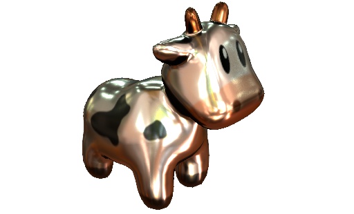 |
|
| Diffuse | Plastic | Metallic | |
| Cosine sampling | 46.81 | 34.88 | 25.61 |
| BSDF sampling | 46.81 | 34.78 | 31.66 |
| Light sampling | 42.70 | 34.23 | 24.38 |
| MIS | 46.50 | 35.40 | 35.82 |
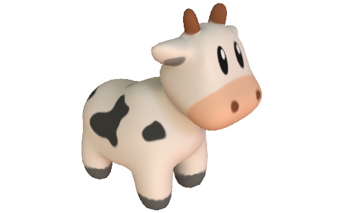
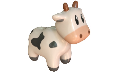
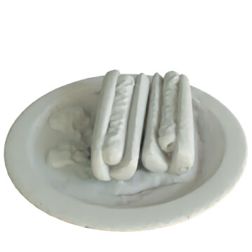
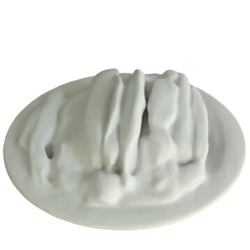
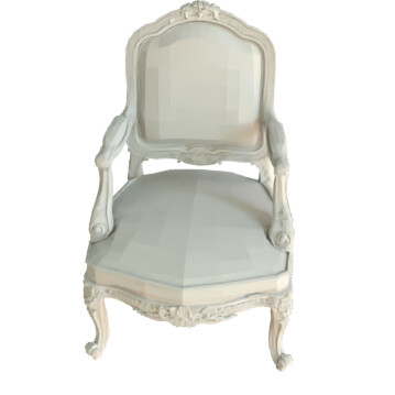
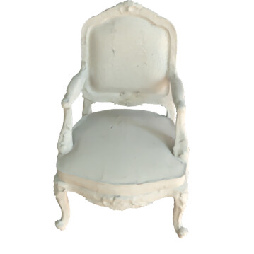
In Figure 18, we examine the effect of importance sampling strategies on reconstruction quality. We compare cosine sampling, BSDF importance sampling [23], light probe importance sampling (using piecewise-constant 2D distribution sampling [48]), and multiple importance sampling [58] (MIS) using the balance heuristic. MIS consistently generates high quality reconstruction for a wide range of materials.
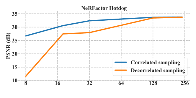
For unbiased results, the forward and backward passes of the renderer should use independent (decorrelated) random samples. However, we observe drastically reduced noise levels, hence improved convergence rates, when using correlated samples, i.e., re-using the same random seeds in the forward and backward pass, especially for low sample count optimization runs. This effect mainly stems from gradients flowing back to the exact same set of parameters which contributed to the forward rendering, instead of randomly selecting another set of parameters, which naturally increases variance. In Figure 19, we compare the two approaches over a range of sample counts.
|
Hotdog |
 |
 |
 |
 |
|---|---|---|---|---|
| 66k tris | 57k tris | 57k tris | 725k tris | |
|
Chair |
 |
 |
 |
 |
| 259k tris | 101k tris | 102k tris | 353k tris | |
|
Lego |
 |
 |
 |
 |
| 2035k tris | 104k tris | 111k tris | 498k tris | |
| Reference | Our | nvdiffrec | PhySG |
Appendix E Geometry
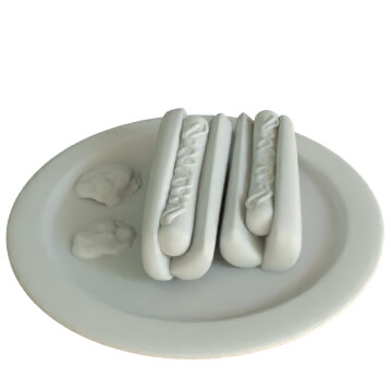
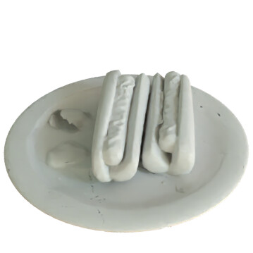
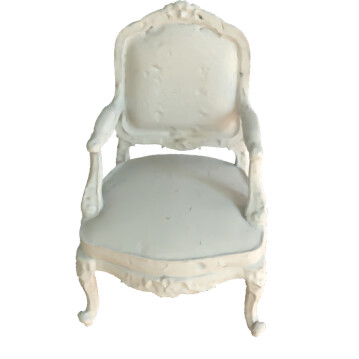
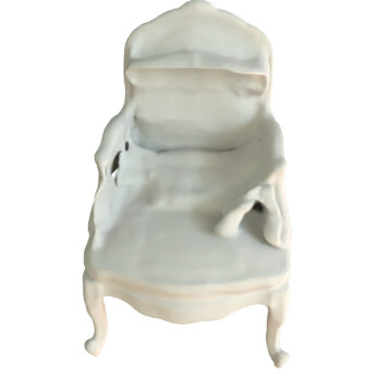
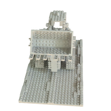
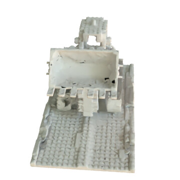
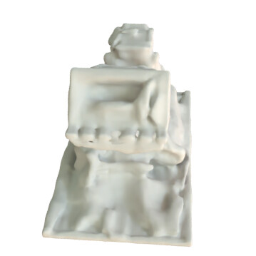
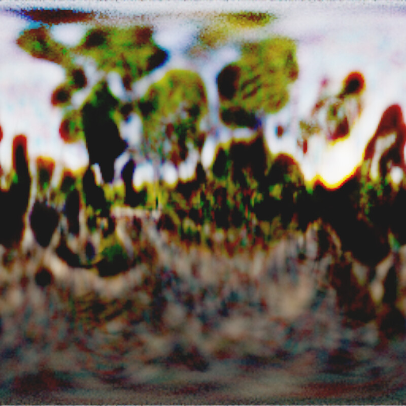
In Table 3 we relate our method to Table 8 (supplemental) of the nvdiffrec paper [41], and note similar geometric quality as nvdiffrec. The Lego scene is an outlier caused by our normal smoothness regularizer from Eq. 9. The scene is particularly challenging for geometric smoothing since it contains very complex geometry full of holes and sharp edges. Please refer to Figure 20 for a visual comparison.
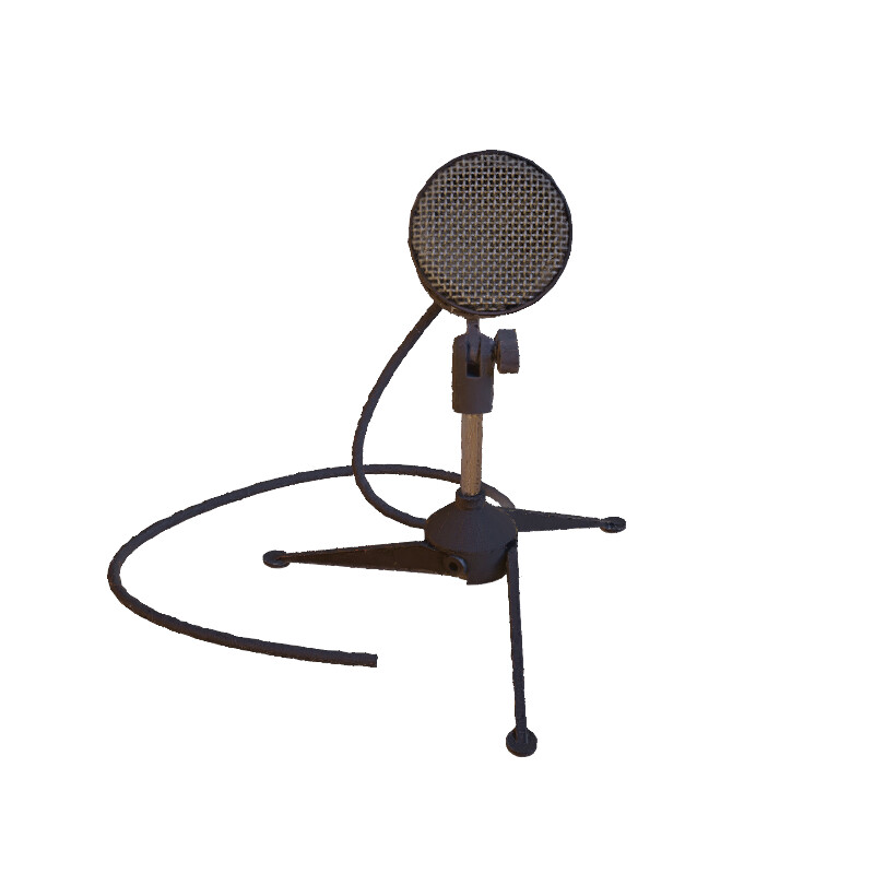
| Chair | Hotdog | Lego | Materials | Mic | |
|---|---|---|---|---|---|
| PhySG | 0.1341 | 0.2420 | 0.2592 | N/A | 0.2712 |
| NeRF (w/o mask) | 0.0185 | 4.6010 | 0.0184 | 0.0057 | 0.0124 |
| NeRF (w/ mask) | 0.0435 | 0.0436 | 0.0201 | 0.0082 | 0.0122 |
| nvdiffrec | 0.0574 | 0.0272 | 0.0267 | 0.0180 | 0.0098 |
| Our | 0.0566 | 0.0297 | 0.0583 | 0.0162 | 0.0151 |
Appendix F Relighting and View Interpolation
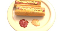
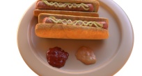
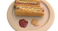
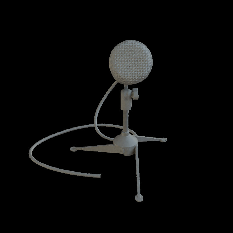
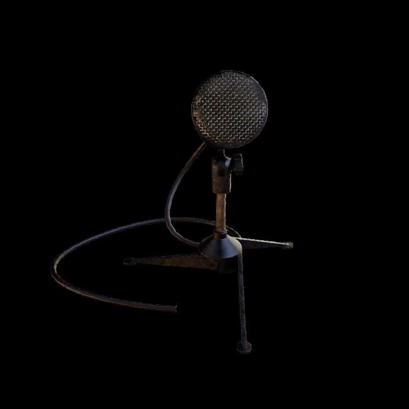
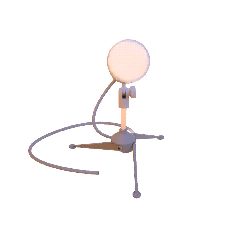
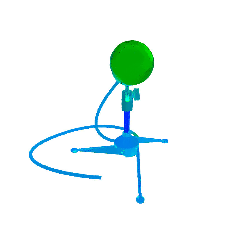
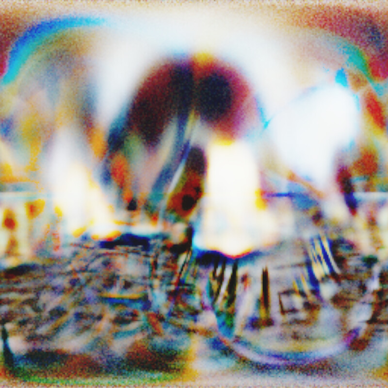
We present relighting results with per scene breakdown for all synthetic datasets in Table 4. Figures 21, 22, and 23 show visual examples of the NeRFactor synthetic dataset. This dataset is intentionally designed to simplify light and material separation (low frequency lighting, no prominent shadowing, direct lighting only). Figures 24, 25, and 26 show visual examples from the NeRF synthetic dataset. This dataset was designed view-interpolation, and contains particularly hard scenes with all-frequency lighting. Table 5 presents per-scene view interpolation scores for the synthetic datasets.
| NeRFactor synthetic dataset | ||||||||||||
| PSNR | SSIM | LPIPS | ||||||||||
| Drums | Ficus | Hotdog | Lego | Drums | Ficus | Hotdog | Lego | Drums | Ficus | Hotdog | Lego | |
| Our | 23.6 | 29.3 | 30.0 | 21.2 | 0.926 | 0.968 | 0.952 | 0.853 | 0.062 | 0.025 | 0.040 | 0.113 |
| nvdiffrec | 22.4 | 27.8 | 29.5 | 19.4 | 0.915 | 0.962 | 0.936 | 0.825 | 0.066 | 0.028 | 0.048 | 0.109 |
| NeRFactor | 21.6 | 21.6 | 25.5 | 20.3 | 0.911 | 0.921 | 0.916 | 0.839 | 0.065 | 0.075 | 0.087 | 0.121 |
| NeRF synthetic dataset | |||||||||||||||
| PSNR | SSIM | LPIPS | |||||||||||||
| Chair | Hotd. | Lego | Mats. | Mic | Chair | Hotd. | Lego | Mats. | Mic | Chair | Hotd. | Lego | Mats. | Mic | |
| Our | 27.0 | 25.9 | 23.4 | 25.1 | 30.9 | 0.946 | 0.929 | 0.890 | 0.923 | 0.972 | 0.044 | 0.073 | 0.088 | 0.047 | 0.025 |
| nvdiffrec | 25.1 | 20.3 | 21.4 | 19.9 | 29.7 | 0.921 | 0.853 | 0.861 | 0.847 | 0.967 | 0.060 | 0.126 | 0.089 | 0.079 | 0.026 |
| Our synthetic dataset | |||||||||
| PSNR | SSIM | LPIPS | |||||||
| Apollo | Porsche | Roller | Apollo | Porsche | Roller | Apollo | Porsche | Roller | |
| Our | 25.6 | 28.2 | 27.5 | 0.931 | 0.965 | 0.952 | 0.045 | 0.030 | 0.027 |
| nvdiffrec | 24.7 | 26.1 | 20.4 | 0.926 | 0.952 | 0.898 | 0.049 | 0.029 | 0.067 |
| NeRFactor synthetic dataset | ||||||||
| PSNR | SSIM | |||||||
| Drums | Ficus | Hotdog | Lego | Drums | Ficus | Hotdog | Lego | |
| Our | 26.6 | 30.8 | 33.9 | 29.1 | 0.940 | 0.975 | 0.967 | 0.930 |
| nvdiffrec | 28.5 | 31.2 | 36.3 | 30.7 | 0.959 | 0.978 | 0.981 | 0.951 |
| NeRFactor | 24.6 | 23.1 | 31.6 | 28.1 | 0.933 | 0.937 | 0.948 | 0.900 |
| NeRF synthetic dataset | ||||||||||
| PSNR | SSIM | |||||||||
| Chair | Hotdog | Lego | Mats. | Mic | Chair | Hotdog | Lego | Mats. | Mic | |
| Our | 29.0 | 30.4 | 26.8 | 25.7 | 29.0 | 0.947 | 0.942 | 0.917 | 0.913 | 0.963 |
| nvdiffrec | 31.6 | 33.0 | 29.1 | 26.7 | 30.8 | 0.969 | 0.973 | 0.949 | 0.923 | 0.977 |
| Our synthetic dataset | ||||||
| PSNR | SSIM | |||||
| Apollo | Porsche | Roller | Apollo | Porsche | Roller | |
| Our | 23.4 | 28.4 | 25.0 | 0.908 | 0.953 | 0.941 |
| nvdiffrec | 23.9 | 28.5 | 25.1 | 0.923 | 0.958 | 0.951 |
|
Ref |
 |
 |
 |
 |
 |
 |
|---|---|---|---|---|---|---|
|
Our |
 |
 |
 |
 |
 |
 |
|
nvdiffrec |
 |
 |
 |
 |
 |
 |
|
NeRFactor |
 |
 |
 |
 |
 |
 |
|
Probes |
||||||
| City | Courtyard | Forest | Studio | Sunrise | Sunset |
|
Ref |
 |
 |
 |
 |
 |
 |
|---|---|---|---|---|---|---|
|
Our |
 |
 |
 |
 |
 |
 |
|
nvdiffrec |
 |
 |
 |
 |
 |
 |
|
NeRFactor |
 |
 |
 |
 |
 |
 |
| City | Courtyard | Forest | Studio | Sunrise | Sunset |
|
Ref |
 |
 |
 |
 |
 |
 |
|---|---|---|---|---|---|---|
|
Our |
 |
 |
 |
 |
 |
 |
|
nvdiffrec |
 |
 |
 |
 |
 |
 |
|
NeRFactor |
 |
 |
 |
 |
 |
 |
| City | Courtyard | Forest | Studio | Sunrise | Sunset |
|
Ref |
||||
|---|---|---|---|---|
|
Our |
||||
|
nvdiffrec |
||||
|
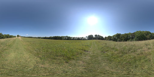
Probes |
 |
 |
 |
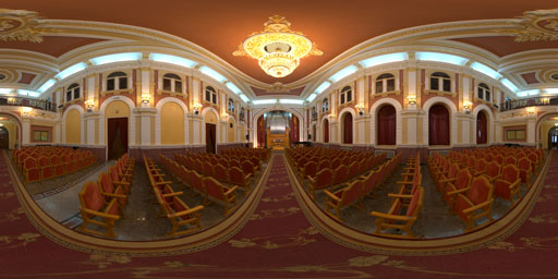 |
| Aerodynamics Workshop | Boiler room | Dreifaltigkeitsberg | Music hall |
|
Ref |
||||
|---|---|---|---|---|
|
Our |
||||
|
nvdiffrec |
||||
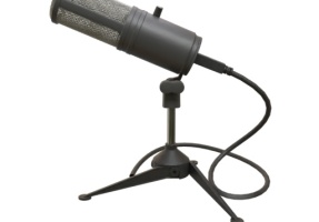
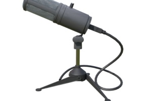
| Aerodynamics Workshop | Boiler room | Dreifaltigkeitsberg | Music hall |
|
Ref |
 |
 |
 |
 |
|---|---|---|---|---|
|
Our |
 |
 |
 |
 |
|
nvdiffrec |
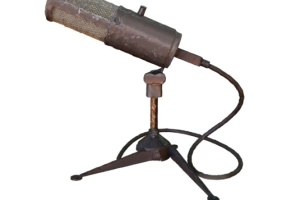 |
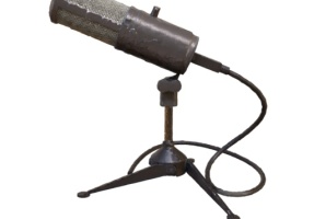 |
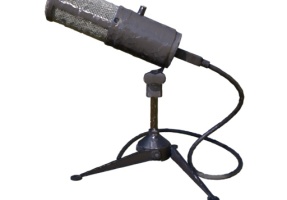 |
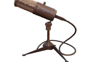 |
| Aerodynamics Workshop | Boiler room | Dreifaltigkeitsberg | Music hall |
| Shaded | Diffuse light | Specular light | Probe | ||
|
w/ reg 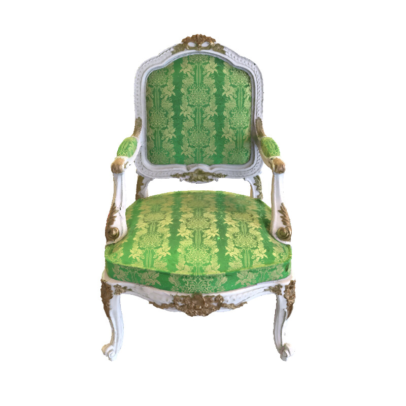
|
 |
 |
 |
 |
 |
|
w/o reg 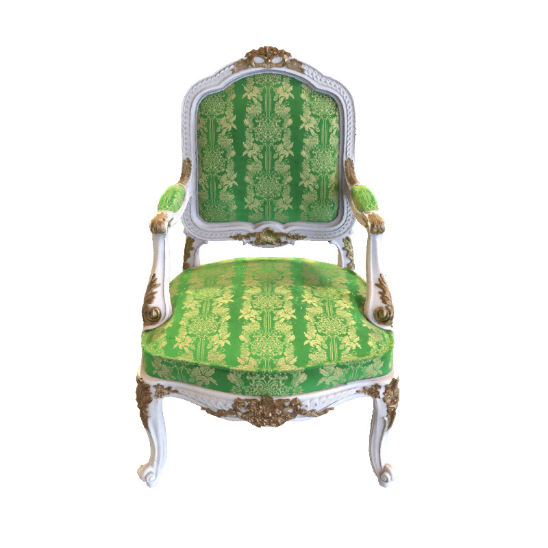
|
 |
 |
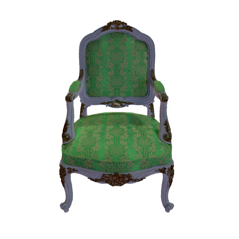 |
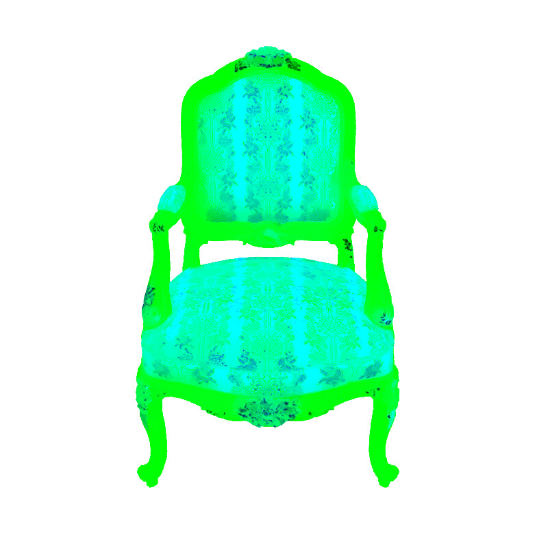 |
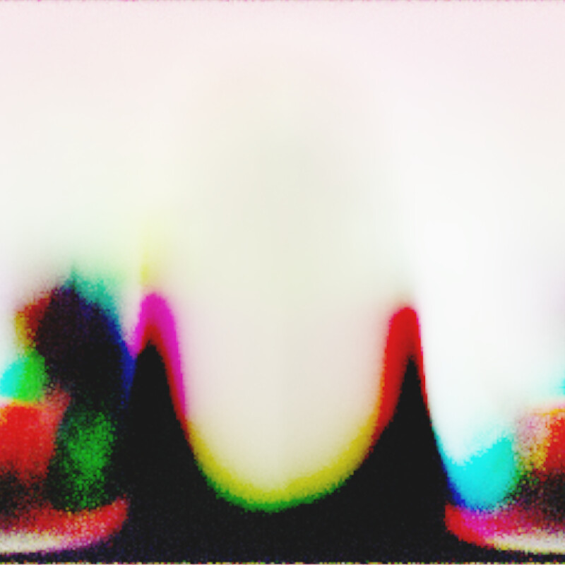 |
|
w/ reg 
|
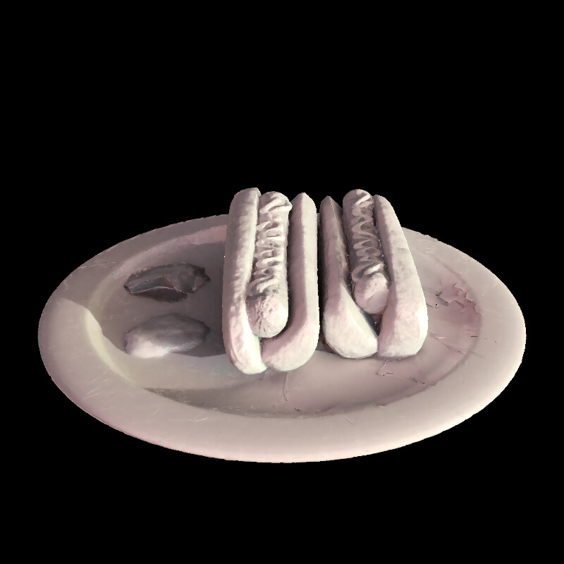 |
 |
 |
 |
 |
|
w/o reg 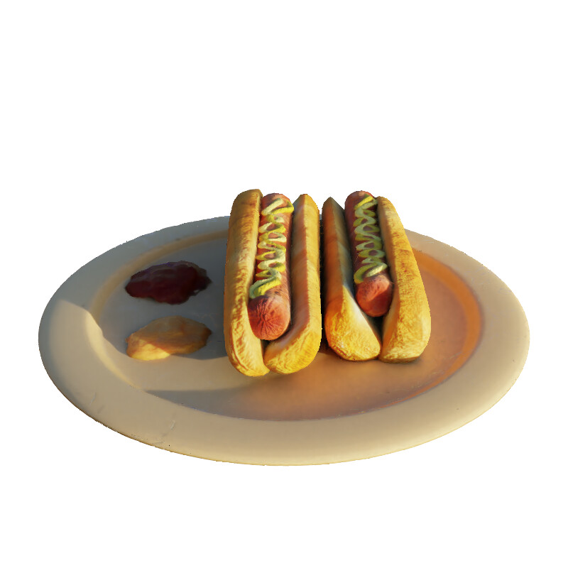
|
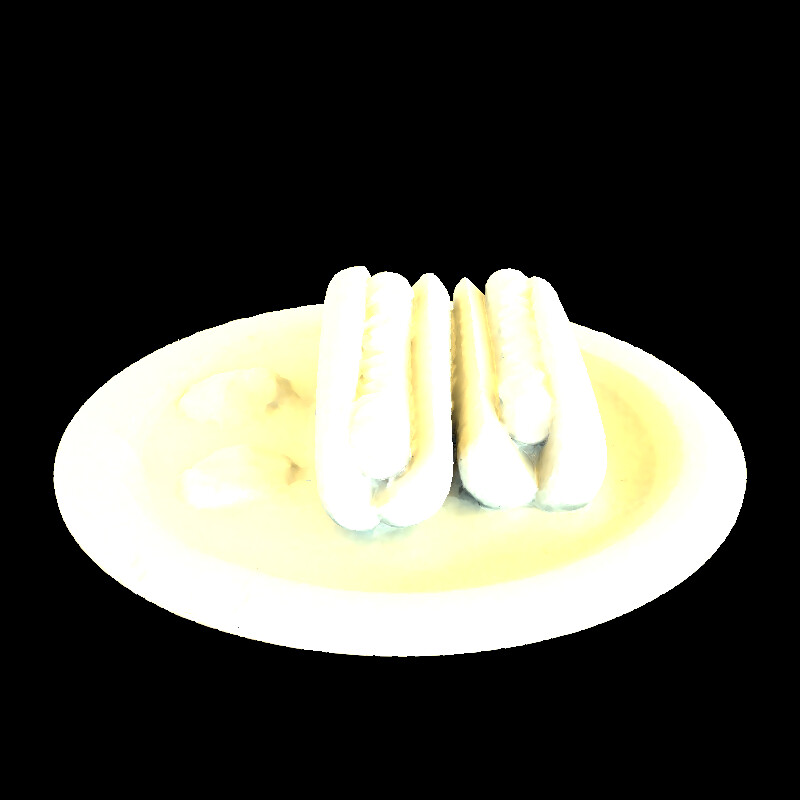 |
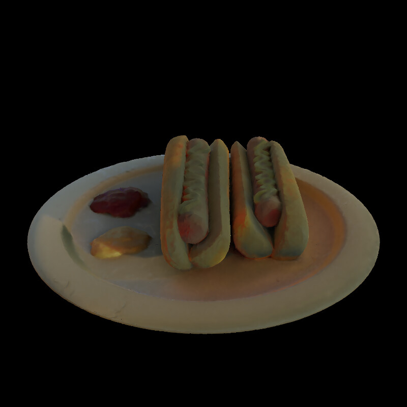 |
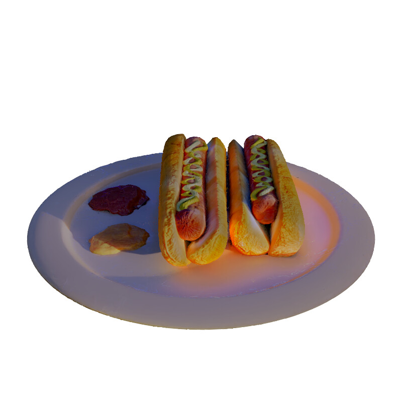 |
 |
 |
|
w/ reg 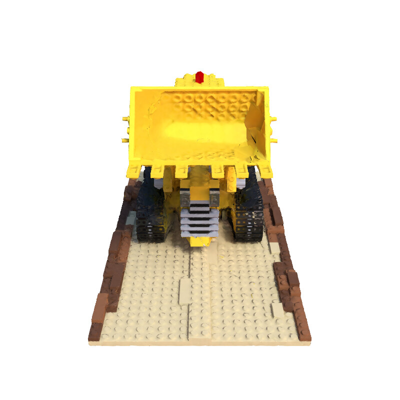
|
 |
 |
 |
 |
 |
|
w/o reg 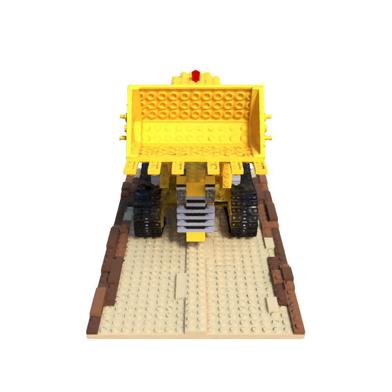
|
 |
 |
 |
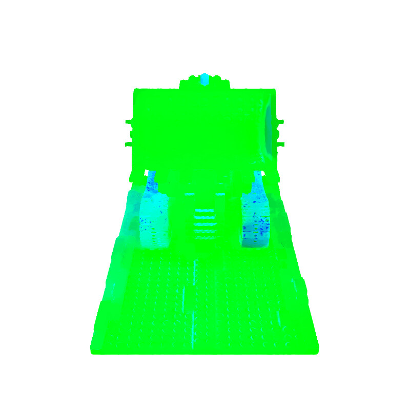 |
 |
|
w/ reg 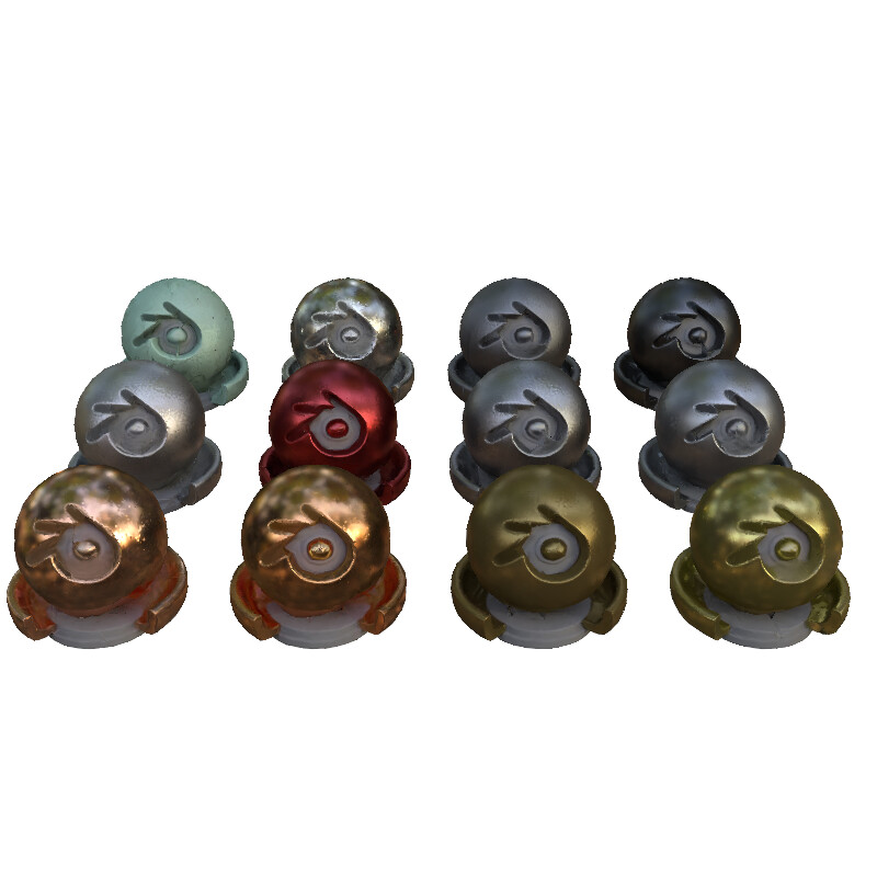
|
 |
 |
 |
 |
 |
|
w/o reg 
|
 |
 |
 |
 |
 |
|
w/ reg 
|
 |
 |
 |
 |
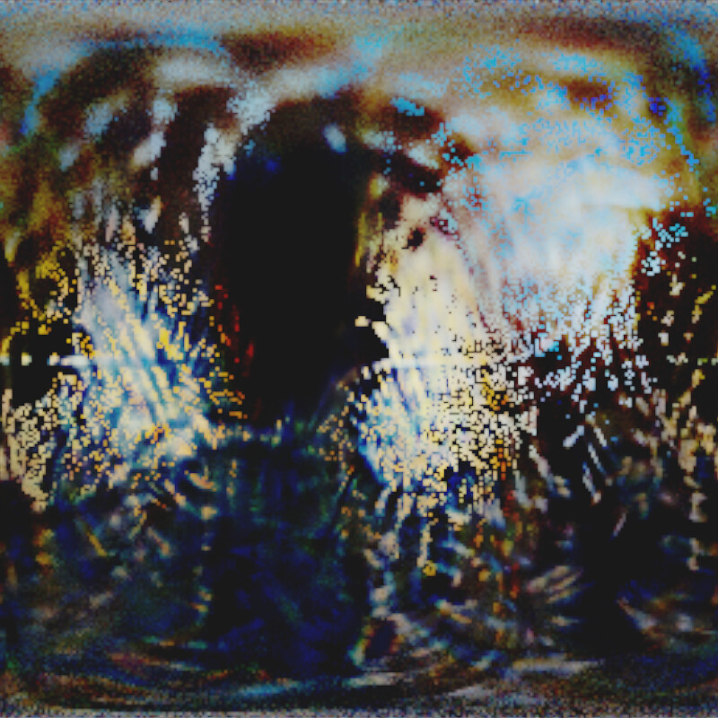 |
|
w/o reg 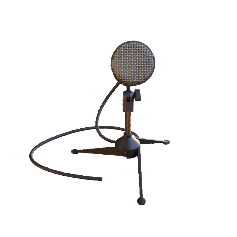
|
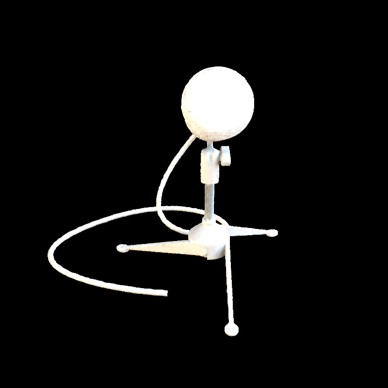 |
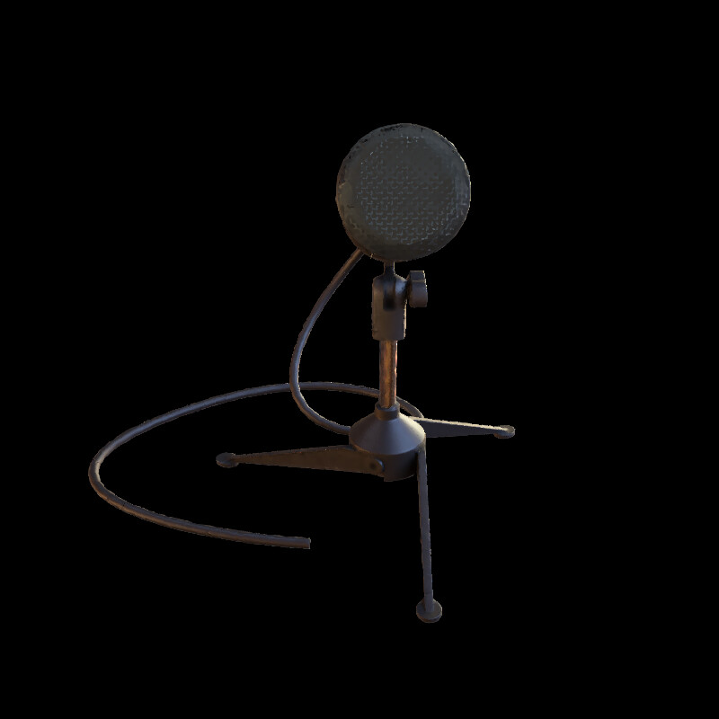 |
 |
 |
 |
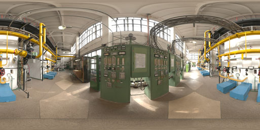
Appendix G Scene Credits
Mori Knob from Yasotoshi Mori (CC BY-3.0). Bob model (CC0) by Keenan Crane. Rollercoaster and Porsche scenes from LDraw resources (CC BY-2.0) by Philippe Hurbain. Apollo and Damicornis models courtesy of the Smithsonian 3D repository [55] (CC0). The Family scene is part of the Tanks&Temples dataset [27] (CC BY-NC-SA 3.0), the Character scene is part of the BlendedMVS dataset [67] (CC BY-4.0) and the Gold Cape scene is part of the NeRD dataset [6] (CC BY-NC-SA 4.0). The NeRF [39] and NeRFactor [75] datasets (CC BY-3.0) contain renders from modified blender models located on blendswap.com: chair by 1DInc (CC0), drums by bryanajones (CC-BY), ficus by Herberhold (CC0), hotdog by erickfree (CC0), lego by Heinzelnisse (CC-BY-NC), materials by elbrujodelatribu (CC0), mic by up3d.de (CC0), ship by gregzaal (CC-BY-SA). Light probes from Poly Haven [70]: Aerodynamics workshop and Boiler room by Oliksiy Yakovlyev, Dreifaltkeitsberg by Andreas Mischok, and Music hall by Sergej Majboroda (all CC0). The probes provided in the NeRFactor dataset are modified from the probes (CC0) shipped with Blender.
