Hierarchical Similarity Learning for Aliasing Suppression Image Super-Resolution

Abstract

As a highly ill-posed issue, single image super-resolution (SISR) has been widely investigated in recent years. The main task of SISR is to recover the information loss caused by the degradation procedure. According to the Nyquist sampling theory, the degradation leads to aliasing effect and makes it hard to restore the correct textures from low-resolution (LR) images. In practice, there are correlations and self-similarities among the adjacent patches in the natural images. This paper considers the self-similarity and proposes a hierarchical image super-resolution network (HSRNet) to suppress the influence of aliasing. We consider the SISR issue in the optimization perspective, and propose an iterative solution pattern based on the half-quadratic splitting (HQS) method. To explore the texture with local image prior, we design a hierarchical exploration block (HEB) and progressive increase the receptive field. Furthermore, multi-level spatial attention (MSA) is devised to obtain the relations of adjacent feature and enhance the high-frequency information, which acts as a crucial role for visual experience. Experimental result shows HSRNet achieves better quantitative and visual performance than other works, and remits the aliasing more effectively.

I Introduction

Image super-resolution is a classical issue in image processing area [1]. Given a low-resolution (LR) image, the task of single image super-resolution (SISR) is to find the corresponding high-resolution (HR) instance with refined details. SISR has been considered in different applications, such as video/image compression, object detection and semantic segmentation.

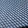
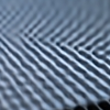
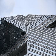
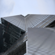
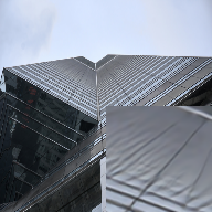
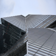
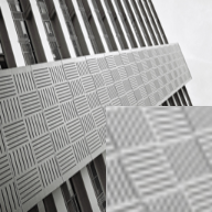
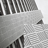
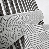
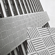
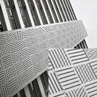
As a highly ill-posed issue, there is numerous information loss caused by the degradation. According to the Nyquist sampling theory [2], the degradation procedure decreases the signal frequency and leads to aliasing, which makes it hard to recover the correct textures. An example of this effect is shown in Figure 1. The higher positions of the building contain plentiful high frequency information and suffer severer aliasing after degradation. The texture mixture makes it hard to find the accurate structural textures.

Fortunately, there are correlations and self-similarities among the adjacent patches in the natural images, and the frequency change in natural image is continuous and smooth. In this point of view, the adjacent patches with lower frequency information is helpful to restore the high frequency information and suppress the aliasing. Figure 1 provides an example of this hypothesis. The textures in the building are similar. From the bottom to the top, the lines becomes dense, and the frequency gets higher. As such, a refined local image prior can be a good guidance to restore the high-frequency areas.

Recently, convolutional neural network (CNN) has proved to be an effective design for exploring the inherent correlations of features and restoring the missing information. SRCNN [3] is the first CNN-based work for SISR problem. After SRCNN, VDSR [4], EDSR [5], LapSRN [6], and other works with elaborate designs builds the network deeper and wider to boost the network representation and restoration capacity. These works focus on elaborate block designs and utilize straightforward networks to recover the missing textures, which seldom concentrate on the local image prior.

There are also CNN-based works recovering the degraded images with the help of external information. Reference-based image super-resolution (RefSR) is also a feasible methodology to restore the degraded images, which requires an extra image as prior guidance for texture recovery. Traditional example-based methods have been considered for image restoration [7, 8, 9] with good visualization performance. There are also deep learning based works for effective texture transfer [10, 11]. Although the reference can give an outstanding prior for recovering the missing information, there are two critical issues for RefSR to restore the correct textures. On one hand, the quality of reference image directly influences the performance of restoration. On the other hand, different from the self-similarity in nature image, the provided reference image contains diverse information for restoration, and leads to excrescent and incorrect textures.

In this paper, we aim to find a formula solution for the SISR problem in the optimization perspective, and restore the missing information with the help of similarity learning. Specifically, we design an iterative SISR network based on the half-quadratic splitting (HQS) strategy. To consider the local image prior, a hierarchical exploration block (HEB) is proposed to explore the texture feature. The hierarchical exploration in HEB progressively recovers the missing texture by filters with incremental receptive fields and gradually enlarges the local information prior. Besides the hierarchical exploration, a multi-level spatial attention (MSA) is designed to address the adjacent spatial correlation of feature and concentrate more on high-frequency information. Based on the optimization-based network backbone and the advanced block designs, we design an hierarchical image super-resolution network termed as HSRNet. Experimental results show our HSRNet achieves better quantitative and visual performance than other image SR works. Specially, HSRNet can remit the aliasing more effectively. Figure 1 shows an example visual quality comparison for different SISR methods. In the figure, existing methods [6, 4, 12] recover the correct grids at the lower positions, but fail on the top of the batch. In contrast, HSRNet can recover more accurate lines and textures under heavy aliasing.

(a) Example image from Urban100 [13]

(b) HR (PSNR/SSIM)

(c) LR (18.24/0.6158)

(d) LapSRN [6] (19.54/0.7614)

(e) VDSR [4] (19.49/0.7584)

(f) MSRN [12] (20.28/0.8170)

(g) HSRNet (20.84/0.8285)

Figure 1: Visual quality comparison for different SISR methods.

Our contributions are summarized as follows:

• We consider the image super-resolution in the optimization perspective, and design an end-to-end SISR network for image restoration based on the half-quadratic splitting (HQS) strategy.

• We consider the self-similarity to suppress the aliasing. To fully utilize the local image prior, we design the hierarchical exploration block (HEB) and the multi-level spatial attention (MSA), and devise a hierarchical image super-resolution network (HSRNet).

• Experimental results show our HSRNet achieves better quantitative and visual performance than other image super-resolution works. Specially, HSRNet can remit the aliasing more effectively and recover more accurate structural textures.

II Literature Review

II-A Deep learning for Single Image Super-Resolution

Convolutional neural network (CNN) has been widely utilized in various computer vision tasks and demonstrates its powerful performance. The first CNN-based work is SRCNN [3] with a three-layer neural network, which followed a sparse-coding like structure. After SRCNN, deeper and wider CNNs were proposed for boosting the performance. VDSR [4] built a very deep network with 20 convolutional layers for better restoration capacity. In ESPCN [14], sub-pixel convolution was firstly introduced for up-sampling, and has been widely used in later works. EDSR [5] pointed out that batch normalization is not suitable for SISR problem, and built a very deep network with residual blocks. SRDenseNet [15], inspired by densely connection, also achieved state-ot-the-art performance with well-designed network architecture. RDN [16] combined the residual connection and densely connection, and proposed a residual dense block for effective image restoration. RCAN [17] considered residual-in-residual design for effective information and gradient transmission. Inspired by Laplacian Pyramid, LapSRN [6] firstly proposed a progressive Laplacian network for multiple scale image super-resolution. OISR [18] considered an ODE-Inspired network and achieved good performance. DBPN [19] obtained the back projection method for SISR and designed a network to restore the image. SRFBN [20] also considered feedback and iteration for effective image restoration with restricted parameters. Recently, DAN [21], CS-NL [22], and other works also utilize elaborate network designs and achieve amazing restoration performance.

There are also lightweight works for efficient SISR. CARN [23] utilized a cascading recursive network to restore the image with fast speed. IDN [24] considered information distillation mechanism into image super-resolution and successfully decreased the computation complexity and network parameters. To further investigate the effectiveness of information distillation, IMDN [25] proposed the multi-distillation strategy and achieved state-of-the-art performance. RFDN [26] improved the architecture of IMDN and further boosted the restoration capacity.

Besides effective block designs, attention mechanism has also become an important part for SISR network, which aims to concentrate more on important information and area. As far as we know, channel-wise attention block was firstly proposed in SENet [27] to boost the network representation, and then was utilized in RCAN [17] to concentrate more on important feature channels. RFDN [26] considered an enhanced spatial attention for comprehensive correlation learning. Besides local attentions, CS-NL [22] proposed a cross-scale non-local attention mechanism to achieve the state-of-the-art performance.

II-B Image Super-Resolution in the Optimization View

There are also works considering the problem in the optimization perspective. IRCNN [28] utilized half-quadratic splitting (HQS) strategy and built a network to learn the denoiser prior for image restoration. DPSR [29] proposed a novel degradation model and used HQS to find the closed-form solution. USRNet [30] combined the model-based and learning-based methodologies and proposed a deep unfolding super-resolution network for non-blind SISR. Liu et al. designed ISRN [31] to perform end-to-end image super-resolution inspired by HQS.

Besides HQS, there are other strategies to model the SISR issue and find the solution. Plug-and-Play ADMM [32] has been proposed for image restoration with a plug-and-play denoiser. Deng et al. proposed a deep coupled ISTA network for multi-model image super-resolution [33]. ISTA-Net [34] considered an unfolding network based on the ISTA algorithm, and achieved good performance on compressive sensing and image restoration. ADMM-Net [35] also proposed an ADMM-based network for reconstructing the compressive sensing images.

Figure 2: Network structure of HSRNet. The space transformation is conducted by convolution and upscale. Three components are proposed to perform the optimization

III Methodology

In this section, we will introduce our HSRNet in the following manner. Firstly we will analyze the issue according to HQS strategy, and describe the network design of our HSRNet. Then, the detail of hierarchical exploration block (HEB) and multi-level spatial attention (MSA) will be discussed. Finally, we will talk about the difference between HSRNet and other related works.

III-A Network Design

The observation model of SISR issue is,

$$\mathbf{I}^{LR}=\mathbf{H}\mathbf{I}^{HR}+\mathbf{n},$$ (1)

where $\mathbf{I}^{LR}$, $\mathbf{I}^{HR}$ are corresponding LR and HR instances, $\mathbf{H}$ is the degradation matrix and $\mathbf{n}$ is the noise term. To find $\mathbf{I}^{HR}$ from $\mathbf{I}^{LR}$, based on the observation model, the optimization target of SISR can be written as,

$$\mathbf{I}^{HR}=\arg\min_{\mathbf{I}^{HR}}\frac{1}{2}||\mathbf{I}^{LR}-\mathbf{HI}^{HR}||_{\ell}^{2}+\Phi(\mathbf{I}^{HR}),$$ (2)

where $\Phi(\cdot)$ denotes the prior term for HR images.

Let $\mathbf{u}=\mathbf{I}^{HR}$, according to the HQS strategy, the optimization target can be cast into the iterative solution, as,

$$\left\{\begin{aligned} \mathbf{I}^{HR}_{k+1}&=\arg\min_{\mathbf{I}^{HR}}\frac{1}{2}||\mathbf{I}^{LR}-\mathbf{H}\mathbf{I}^{HR}||_{\ell}^{2}+\frac{\beta_{k}}{2}||\mathbf{I}^{HR}-\mathbf{u}_{k}||^{2}_{\ell},\\ \mathbf{u}_{k+1}&=\arg\min_{\mathbf{u}}\frac{\beta_{k}}{2}||\mathbf{I}^{HR}_{k+1}-\mathbf{u}||^{2}_{\ell}+\Phi(\mathbf{u}),\end{aligned}\right.$$ (3)

where $\beta$ is a constant of penalty term, and increases with the accumulation of iteration times. It should be addressed that the solution of $\mathbf{u}_{k+1}$ has the same situation of a denoising problem, and $\mathbf{I}^{HR}_{k+1}$ has a closed-form least square (LS) solution, where,

$$\mathbf{I}^{HR}_{k+1}=(\mathbf{H}\mathbf{H}^{\mathrm{T}}+\beta\mathbf{I})^{-1}(\mathbf{H}^{\mathrm{T}}\mathbf{I}^{LR}+\beta\mathbf{u}_{k}).$$ (4)

In fact, when $\mathbf{H}$ is hard to be found, or even without explicit mathematical expression, it is challenging to find the solution of Equation (4). A possible strategy is to learn the hidden degradation from training data pairs. In this point of view, Equation (4) should be regarded as a CNN-based function with the input as $\mathbf{H}^{\mathrm{T}}\mathbf{I}^{LR}$ and $\mathbf{u}_{k}$, and the output as $\mathbf{I}^{HR}_{k+1}$. Similarly, the solution of $\mathbf{u}_{k+1}$ can be also considered as a denoiser with the input $\mathbf{I}^{HR}_{k+1}$. As such, Equation (3) can be converted into an iterative CNN-based structure for finding the solution, which can learn the hyper-parameters more effectively.

However, there is a critical issue that both $\mathbf{u}$ and $\mathbf{I}^{HR}_{k}$ are with high resolution, which cause higher computation complexity. In this point of view, a specific space with low resolution should be considered to process the HR images and features. To make the optimization in the low resolution space, we devise the HSRNet to convert the spaces and perform the optimization iteratively.

Figure 2 shows the network structure of HSRNet. Firstly, a convolution converts the input LR image into a specific space, as,

$$\hat{\mathbf{I}}^{LR}=Conv(\mathbf{I}^{LR}),$$ (5)

where $\hat{\cdot}$ means the representation in the specific space.

After space transformation, Transposition module aims to learn the $\mathbf{H}^{\mathrm{T}}$ and performs it on $\hat{\mathbf{I}}^{LR}$, such that,

$$\mathbf{H}^{\mathrm{T}}\hat{\mathbf{I}}^{LR}=Trans(\hat{\mathbf{I}}^{LR}),$$ (6)

where $Trans(\cdot)$ is the Transposition module. As shown in the figure, this module is composed of two convolutional layers and a Leaky ReLU activation.

With the learned $\mathbf{H}^{\mathrm{T}}\hat{\mathbf{I}}^{LR}$, Solver LS and Denoiser are mainly designed to generate the solution of Equation (3) separately. HSRNet performs the iteration for several times. For the $k$-th iteration, there are,

$$\hat{\mathbf{I}}^{HR}_{k+1}=SolverLS(\mathbf{H}^{\mathrm{T}}\hat{\mathbf{I}}^{LR},\hat{\mathbf{u}}_{k}),$$ (7)

and

$$\hat{\mathbf{u}}_{k+1}=Denoiser(\hat{\mathbf{I}}^{HR}_{k+1}).$$ (8)

The Solver LS aims to calculate the least square solution in the specific space by neural network, which is composed of three convolutional layers and a Leaky ReLU. The Denoiser is composed of MSAs and HEBs and a convoluitonal layer, which are sequentially stacked.

Finally, the HR image is restored from the specific space after $K$-th iteration, as,

$$\mathbf{I}^{HR}=Upscale(\hat{\mathbf{I}}^{HR}).$$ (9)

The Upscale module is simply composed of one convolutional layer and a sub-pixel convolution.

In the next sections, we will introduce the designed hierarchical exploration block (HEB) and the multi-level spatial attention (MSA) for HSRNet. The proposed components concentrate on the hierarchical correlations among features and the local image prior for effective aliasing suppression.

III-B Hierarchical Exploration Block

Figure 3: Structure of hierarchical exploration block (HEB).

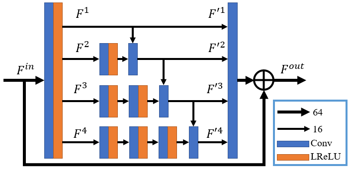
Figure 3 shows the design of HEB. Let $F^{in}$, $F^{out}$ denote the input and output features separately. One convolution with LeakyReLU firstly explore the input feature, as,

$$F^{feat}=f(F^{in}),$$ (10)

where $f(\cdot)$ denotes the feature exploration operation by one convolution with LeakyReLU.

After exploration, the feature $F^{feat}$ is separated into four features with equal channel number. This separation is described as,

$$[F^{1},F^{2},F^{3},F^{4}]=F^{feat},$$ (11)

where $F^{feat}$ is with 64 channels, while $\{F^{i}\}_{i=1}^{4}$ are with 16 channels.

As shown in Figure 3, the four separated features are processed with different receptive fields for further hierarchical information aggregation. For $F^{1}$, there is no operation and the identical information is preserved. The processed feature is considered as,

$$F^{\prime 1}=F^{1}.$$ (12)

For the $i$-th feature $F^{i}$ where $i\geq 2$, it will be firstly explored for $(i-1)$ times to increase the receptive field, and then combined with $F^{\prime i-1}$ to consider the neighborhood information. This exploration can be described as,

$$F^{\prime i}=Conv([f^{i-1}(F^{i}),F^{\prime i-1}]),$$ (13)

where $f^{i-1}$ means perform the exploration for $(i-1)$ times.

Finally, the hierarchical features will be concatenated for jointly consideration. The output feature of HEB is,

$$F^{out}=F^{in}+Conv([F^{\prime 1},F^{\prime 2},F^{\prime 3},F^{\prime 4}]).$$ (14)

(a) Laplacian Pyramid

(b) Hierarchical Exploration in HEB

Figure 4: Comparison between the hierarchical exploration in HEB and the Laplacian Pyramid.

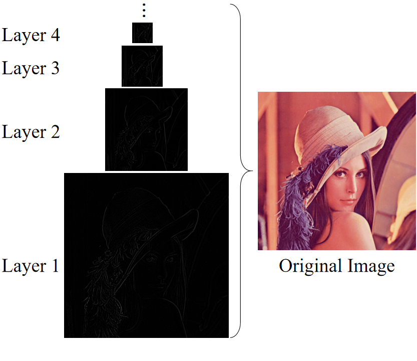
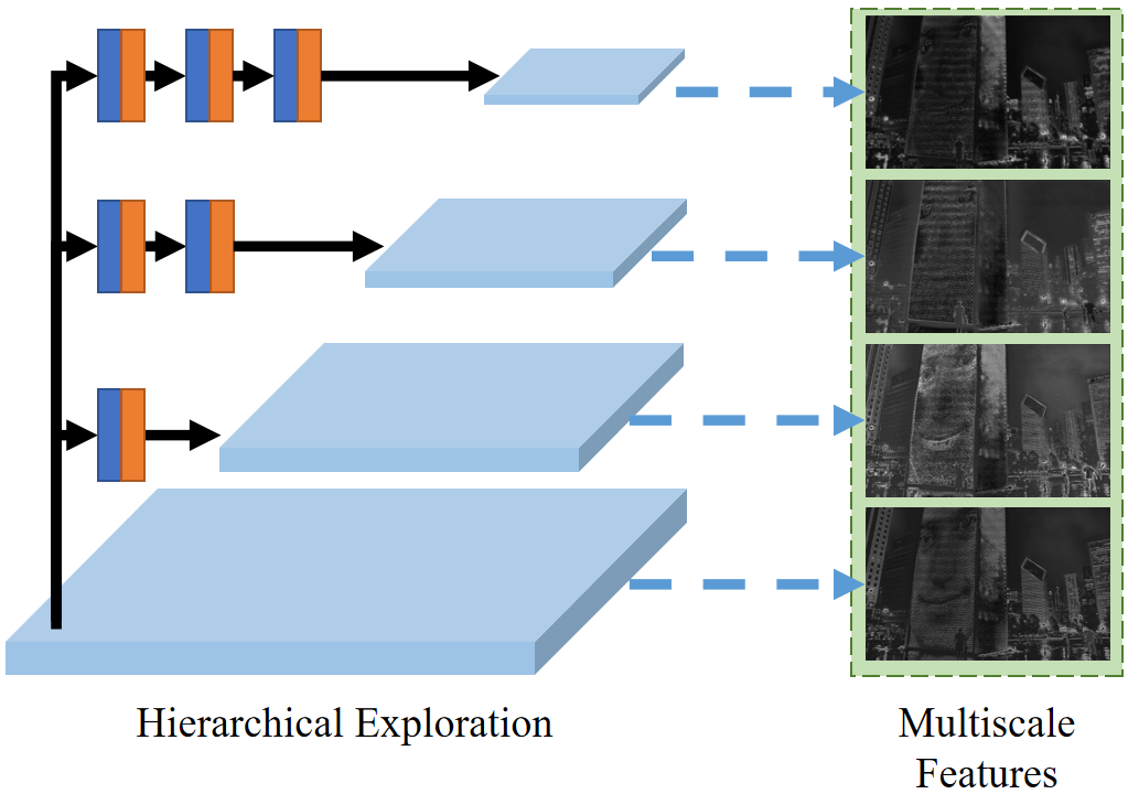
The HEB obtains the local image prior in a progressive manner. With the increase of feature index $i$, the receptive field becomes larger and more adjacent information is considered to restore the mixed textures. The hierarchical exploration strategy in HEB has a similar structure to the Laplacian Pyramid. Figure 4 shows the comparison between the hierarchical exploration in HEB and the Laplacian Pyramid.

With the increase of pyramid layer, the Laplacian Pyramid focuses more on the global information. This is in accordance with the hierarchical exploration in the HEB. In the Figure 4 (a) we can find that the Laplacian Pyramid separates the original image into several layers. The first layer contains the most details information of the image. With the increase of the layer, the residual maps have higher responses on the global information. Similarly, we conduct the hierarchical exploration in HEB by stacking different numbers of the convolutional layers. With the increase of convolutional layers, the receptive field becomes larger, and the structural and larger scale information is gradually addressed.

Different from the Laplacian Pyramid that downsamples the image by interpolation and Gaussian blur, the HEB utilizes convolutional layers to increase the receptive field without changing the resolution of the feature map. HEB can adaptively learn the downscaling parameters in the training step, and produces clearer and suitable features for restoration. It should be noticed there is a concatenation operation between features from different scales in the HEB. With the help of the multi-scale information, structural information from adjacent patches is gradually addressed to consider the local similarity and recover the missing textures.

III-C Multi-level Spatial Attention

Figure 5: Structure of multi-level spatial attention (MSA).

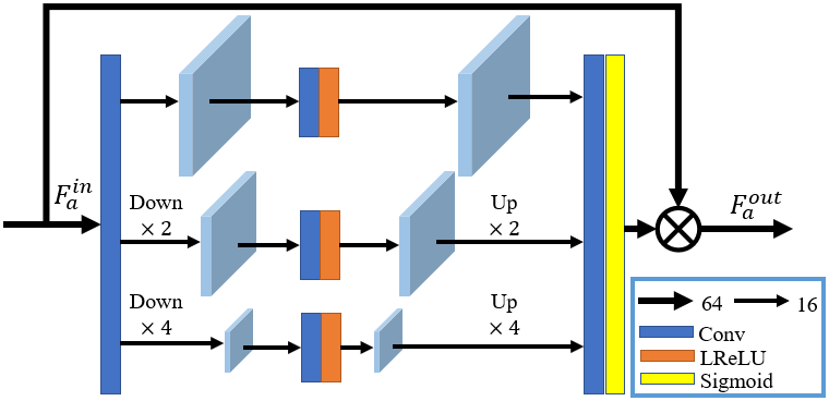
Besides the feature exploration, attention mechanism is devised to concentrate more on the important area and complex information. Let $F^{in}_{a}$, $F^{out}_{a}$ denote the input and output features of MSA separately. The input feature is firstly processed and separated into three features with equal channel number, which is described as,

$$[F_{a}^{1},F_{a}^{2},F_{a}^{3}]=Conv(F^{in}_{a}),$$ (15)

where $F_{a}^{1}$, $F_{a}^{2}$, and $F_{a}^{3}$ are with 16 channels, and $F^{in}_{a}$ is with 64 channels.

After separation, max-pooling is performed on features with different scaling factors to obtain the multi-level spatial representation. One convolution with LeakyReLU is utilized to explore the multi-level feature. Then, bilinear interpolation is utilized to upscale the features, and keep the shapes before and after multi-level exploration. This operation can be described as,

$$F^{\prime 1}_{a}=f(F^{1}_{a}),$$ (16)

$$F^{\prime 2}_{a}=(f((F^{2}_{a})\downarrow_{\times 2}))\uparrow_{\times 2},$$ (17)

$$F^{\prime 3}_{a}=(f((F^{3}_{a})\downarrow_{\times 4}))\uparrow_{\times 4},$$ (18)

where $(\cdot)\downarrow$ means the max pooling, $(\cdot)\uparrow$ means the bilinear upsampling, and $f(\cdot)$ denotes the feature exploration operation by one convolution and a Leaky ReLU.

After multi-level exploration, the spatial features are aggregated and processed to obtain the attention map. Finally, the output of MSA is,

$$F_{a}^{out}=\sigma(Conv([F^{\prime 1}_{a},F^{\prime 2}_{a},F^{\prime 3}_{a}])),$$ (19)

where $\sigma(\cdot)$ is the Sigmoid activation.

Figure 6: Visualized feature maps of hierarchical exploration. (a): input image. (b): $F^{1}$ in Eq. (12). (c)-(e): the processed features with different receptive fields, which denote $f^{1}(F^{2})$ to $f^{3}(F^{4})$ in Eq.(13) separately. (f)-(h): the explored features with different scales, which denote $F^{\prime 2}$ to $F^{\prime 4}$ in Eq.(13) separately. According to the visualization results, the structural and high-frequency information is gradually addressed, which is in accordance with the local image prior for feature exploration.

IV Experiment

IV-A Settings

In HSRNet, the convolutional layers in Transposition and Solver LS are set with 64 filters. There are $N=10$ blocks in the Denoiser module, and $K=3$ iterations for optimization. We train the network for 1000 epochs by Adam optimizer with learning rate $lr=10^{-4}$. The loss function is chosen as L1-loss.

We use DIV2K [36] dataset to train the network. DIV2K is a high resolution dataset for image SR, which contains 900 instances with 2K resolution. We use the peak signal-to-noise ratio (PSNR) and structural similarity (SSIM) to measure the restoration performance. Five testing benchmarks are chosen to compare the performance: Set5 [37], Set14 [38], BSD100 [39], Urban100 [13] and Manga109 [40]. The patch size is chosen as $48\times 48$ for the LR input, and the scaling factors are chosen as $\times 2$, $\times 3$ and $\times 4$. The degradation operation is chosen as bicubic down (BI).

IV-B Model Analysis

IV-B1 Investigation on the Optimization Modules

Figure 7: Visualized feature maps of the input of the Solver LS, the input of the Denoiser, and the output of the Denoiser from different iterations. Zoom up for better view.

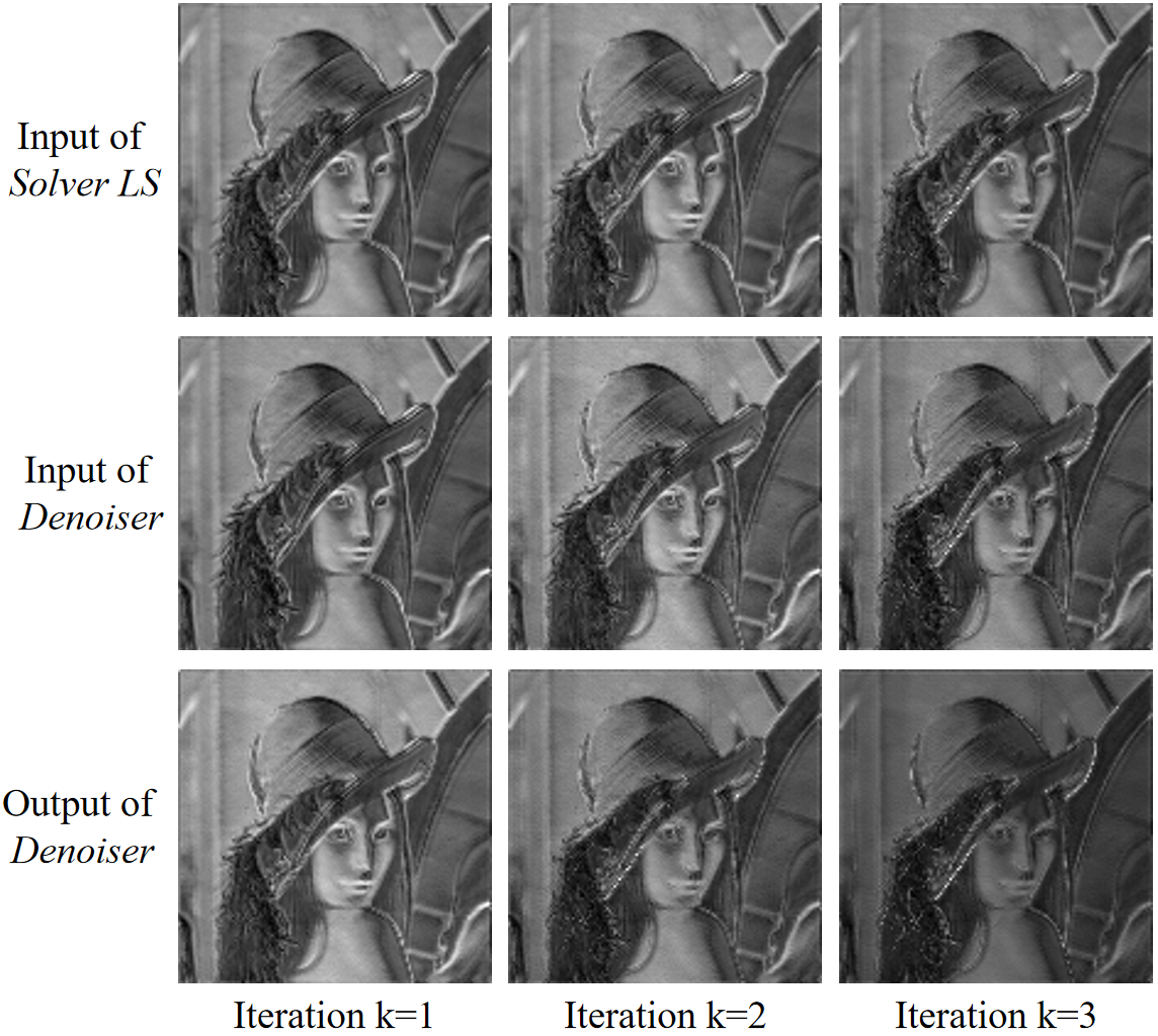
In this section, we verify the functions of the proposed modules with showing the feature maps. The feature maps of the input of the Solver LS, the input of the Denoiser, and the output of the Denoiser are shown in Figure 7. We choose the maximum values of different channels in the feature maps for visualization, which are normalized in range $0$ to $1$. It should be noticed that the input of the Denoiser is just the output of the Solver LS. In this point of view, every three feature maps in the same column are produced sequentially by the modules. Every three feature maps in the same row are produced by the same module from different iterations.

For each row of the figure, we can find that the feature maps become clearer with the increase of the iteration. This is in accordance with the optimization scheme. For each column of the figure, the features are sequentially processed by the Solver LS and the Denoiser. We can find that the Solver LS reduces the artifacts and jaggies of the edges. The jaggies are introduced by the $\mathbf{H}^{\mathrm{T}}\hat{\mathbf{I}}^{LR}$ in the Equation (7), which contains the low-resolution information. Solver LS restores the high-resolution information and preserves the fidelity for the input feature maps, which can be regarded as a feasible solution dominated by the $\mathbf{H}^{\mathrm{T}}\hat{\mathbf{I}}^{LR}$ and the $\hat{\mathbf{u}}$. The Denoiser further suppresses the response of the low-frequency areas and the jaggies, and enhances the edges and lines. The structures at the back of the human become sharper after the Denoiser. Besides, the responses of the edges of the hat and the human become higher after the Denoiser. As such, the Denoiser finds a feasible solution of $\hat{\mathbf{u}}$ with higher responses on the structural information.

(a)

(b)

(c)

(d) (a) Scaling Factor $\times 2$

(e) (b) Scaling Factor $\times 3$

(f) (c) Scaling Factor $\times 4$

Figure 8: Visualized feature maps of $\hat{\mathbf{I}}^{LR}$ from different scales.

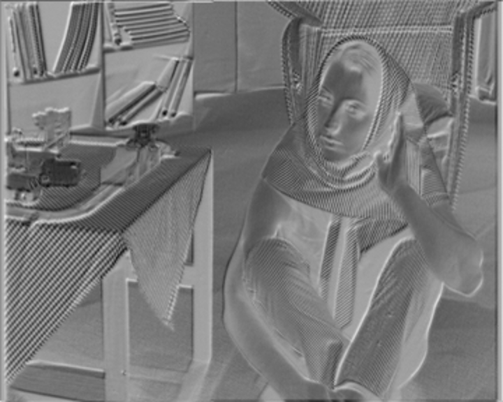
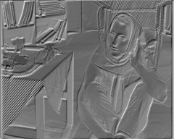
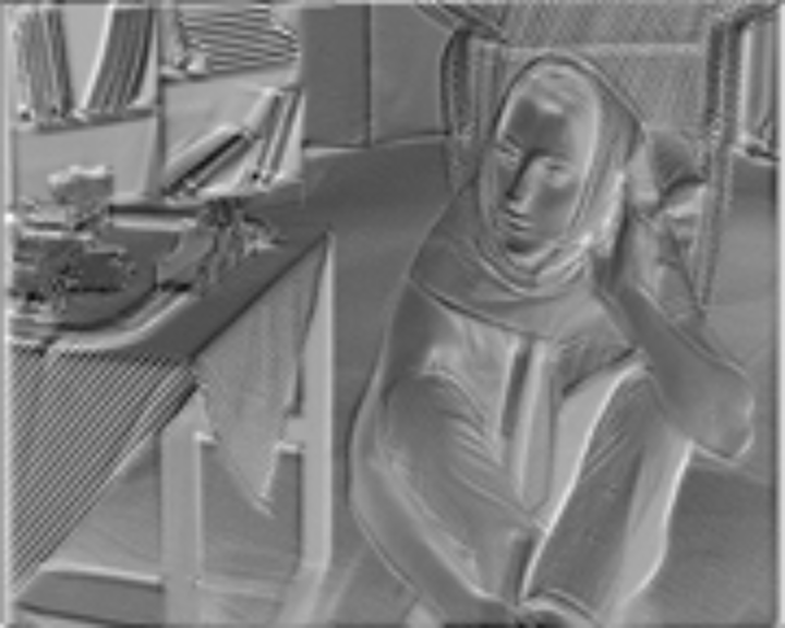
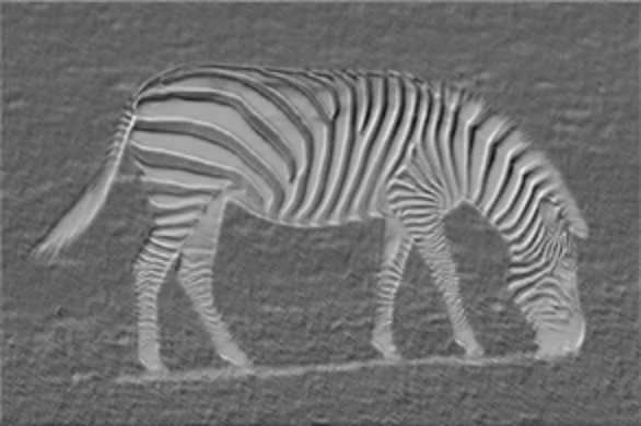
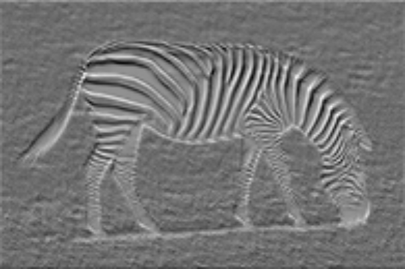
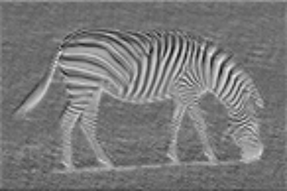
There is one convolutional layer at the begin of the network. The convolution converts the image into feature maps with the same size of $\mathbf{I}^{LR}$. By using this conversion, we can effectively reduce the computation cost. With the increase of scaling factors, the resolution of LR images becomes smaller, and the information is limited.

To analyze the effectiveness of different scaling factors, we compare the feature maps from differnet LR inputs and restore them to the same resolution. The visualized feature maps are $\hat{\mathbf{I}}^{LR}$ in the Equation (5). We calculate the average response of different channels and normalize them in range 0 to 1. The visualized feature maps with different scaling factors are shown in the Figure 8.

In the figure, we can find that the features become blurry and the information is lost with the increase of scaling factors. The textures of tablecloth and the scarf in the first row are missing when the scaling factor is larger. Similarly, the stripes on the legs of the zebra are aliased with the increase of the scaling factor.

IV-B2 Investigation on HEB

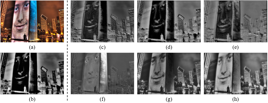
In this section, we mainly investigate the performance of different components in HSRNet. In Section III-B, we argue that HEB obtains a hierarchical exploration to consider the local image prior. Figure 6 illustrates the processed features in different scales. To make the feature maps clear and focus on the effectiveness of network structure, we draw the pictures by the initial random network weights without further training. Figure 6 (a) is the input image. Visualization images from (b) to (e) are the processed feature maps with different receptive fields. We can find the scale of features is larger and larger with the increase of receptive field. The structural textures is gradually addressed, and the high frequency information is dilated to the adjacent patches. For example, the top area of the building in (b) is flat. From (c) to (e), the lines are obvious in the feature map, and dilate to a larger scale. This diffusion phenomenon is in accordance with our local image prior hypothesis, where the refined adjacent patches can provide a good guidance for restoration. To further investigate the effectiveness of local image prior, we visualize the explored features with the guidance of hierarchical information. (b), (f)-(h) in Figure 6 shows the example visualized feature maps of $F^{\prime 1}$ to $F^{\prime 4}$ in Eq.(13) separately. We can find with the increase of scaling factors, the aliasing is gradually suppressed, and the structural information is recovered.

To further investigate the effectiveness of HEB, we build the contrast experiments with different number of the HEB. The numbers of blocks are set with $N=3,5,7$ and we train them under the same protocol. Table I shows the PSNR/SSIM results with different block numbers. The performance is boosted with the increase of $N$.

TABLE I: Investigation on different block numbers on PSNR/SSIM with BI $\times 4$ degradation.

$N$	Set14	B100	Urban100	Manga109
3	28.53/0.7802	27.54/0.7352	25.92/0.7810	30.25/0.9054
5	28.58/0.7818	27.58/0.7365	26.10/0.7868	30.51/0.9085
7	28.66/0.7839	27.63/0.7380	26.21/0.7904	30.69/0.9108
10	28.68/0.7840	27.64/0.7388	26.28/0.7934	30.72/0.9114

IV-B3 Investigation on MSA

(a) (a)

(b) (b)

(c) (c)

(d) (d)

Figure 9: Visualized attention maps from different scales. (a): input image. (b)-(d): attention explored with scaling factor $\times 1$, $\times 2$ and $\times 4$. With the increase of scaling factor, more attentions are aggregated to the high-frequency areas with structural information.

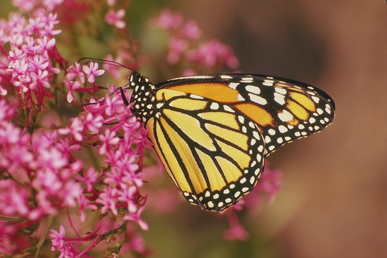
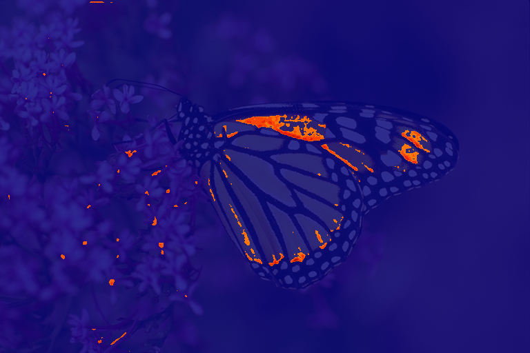
Besides the hierarchical exploration, we also investigate the effectiveness of multi-level spatial attention. In MSA, the multi-level attention aims to concentrate on the important information from different scales. Figure 9 shows the visualized attention maps from different scales. (a) is the original input image. (b)-(d) are the explored attention maps with different scaling factors, which denote $F^{\prime 1}_{a}$ to $F^{\prime 3}_{a}$ in Eq.(16) to (18). In the figure, the receptive field becomes larger and the structural information are highly addressed with the increase of the scaling factor. We can find that in the Figure 9 (b), the attention map holds higher responses on the tiny and dense textures that captured by the small receptive field. When the scaling factor becomes larger, the structural information gets higher attention, such as the wing of the butterfly and the edges of the flowers. In this point of view, the feature map with higher scaling factor concentrates more on the structural information, and the small scaling feature focuses more on the high-frequency tiny details.

TABLE II: Investigation on the attention mechanism on PSNR/SSIM with BI $\times 4$ degradation.

MSA	Set14	B100	Urban100	Manga109
w/o	28.64/0.7827	27.60/0.7371	26.14/0.7886	30.61/0.9091
w	28.68/0.7840	27.64/0.7388	26.28/0.7934	30.72/0.9114

Furthermore, we also investigate the quantitative performance improved by the attention mechanism. Table II shows the PSNR/SSIM comparisons with and without the MSA. From the results, MSA provides near 0.15 dB improvement on Urban100 and 0.1 dB on Manga109. Since Urban100 and Manga109 are high resolution benchmarks with plentiful structural information, the results demonstrate the effectiveness of MSA on the high-frequency texture recovery.

TABLE III: Investigation on the iteration times $K$ on PSNR/SSIM with BI $\times 4$ degradation.

$K$	Set14	B100	Urban100	Manga109
1	28.61/0.7824	27.58/0.7364	26.11/0.7874	30.46/0.9082
2	28.67/0.7838	27.62/0.7377	26.22/0.7909	30.67/0.9105
3	28.68/0.7840	27.64/0.7388	26.28/0.7934	30.72/0.9114

IV-B4 Investigation on Iterative Design

(a) (a)

(b) (b)

(c) (c)

(d) (d)

Figure 10: Restored images from different iteration times $K$. From (a) to (d), the iteration time $K$ is from $0$ to $3$.

As discussed in the network design, we utilize HQS to analyze the image SR in the optimization perspective, and propose an iterative design to find the solution. To investigate the effectiveness of iterative design, we make the contrast comparisons with different iteration times. Table III shows the PSNR/SSIM results with iteration times $K=1,2,3$. In the table, the performance becomes better when $K$ is higher. There is near 0.05 dB PSNR improvement on Manga109 and 0.06 dB improvement on Urban100 when $K=3$.

To further investigate the mechanism of iteration pattern, we compare the restored images from different iteration times. Figure 10 shows the images with $K=1,2,3$. We can find that with the increase of $K$, the details are richer, and the edges on the wing becomes sharper and clearer. This is in accordance with the iteration optimization.

TABLE IV: Average PSNR/SSIM with degradation model BI $\times 2$, $\times 3$, and $\times 4$ on five benchmarks. The best and second performances are shown in bold and underline.

Scale	Model	Set5 [37]	Set14 [38]	B100 [39]	Urban100 [13]	Manga109 [40]
		PSNR/SSIM	PSNR/SSIM	PSNR/SSIM	PSNR/SSIM	PSNR/SSIM
$\times 2$	SRCNN [3]	36.66 / 0.9542	32.42 / 0.9063	31.36 / 0.8879	29.50 / 0.8946	35.74 / 0.9661
	FSRCNN [41]	37.00 / 0.9558	32.63 / 0.9088	31.53 / 0.8920	29.88 / 0.9020	36.67 / 0.9694
	VDSR [4]	37.53 / 0.9587	33.03 / 0.9124	31.90 / 0.8960	30.76 / 0.9140	37.22 / 0.9729
	DRCN [42]	37.63 / 0.9588	33.04 / 0.9118	31.85 / 0.8942	30.75 / 0.9133	37.63 / 0.9723
	LapSRN [6]	37.52 / 0.9590	33.08 / 0.9130	31.80 / 0.8950	30.41 / 0.9100	37.27 / 0.9740
	DRRN [43]	37.74 / 0.9591	33.23 / 0.9136	32.05 / 0.8973	31.23 / 0.9188	37.92 / 0.9760
	MemNet [44]	37.78 / 0.9597	33.28 / 0.9142	32.08 / 0.8978	31.31 / 0.9195	37.72 / 0.9740
	DEGREE [45]	37.58 / 0.9587	33.06 / 0.9123	31.80 / 0.8974	-	-
	CARN [23]	37.76 / 0.9590	33.52 / 0.9166	32.09 / 0.8978	31.92 / 0.9256	38.36 / 0.9765
	IMDN [25]	38.00 / 0.9605	33.63 / 0.9177	32.19 / 0.8996	32.17 / 0.9283	38.88 / 0.9774
	RAN [46]	37.58 / 0.9592	33.10 / 0.9133	31.92 / 0.8963	-	-
	DNCL [47]	37.65 / 0.9599	33.18 / 0.9141	31.97 / 0.8971	30.89 / 0.9158	-
	FilterNet [48]	37.86 / 0.9610	33.34 / 0.9150	32.09 / 0.8990	31.24 / 0.9200	-
	MRFN [49]	37.98 / 0.9611	33.41 / 0.9159	32.14 / 0.8997	31.45 / 0.9221	38.29 / 0.9759
	SeaNet-baseline [50]	37.99 / 0.9607	33.60 / 0.9174	32.18 / 0.8995	32.08 / 0.9276	38.48 / 0.9768
	MSRN [12]	38.08 / 0.9607	33.70 / 0.9186	32.23 / 0.9002	32.29 / 0.9303	38.69 / 0.9772
	HSRNet	38.07 / 0.9607	33.78 / 0.9197	32.26 / 0.9006	32.53 / 0.9320	38.90 / 0.9776
$\times 3$	SRCNN [3]	32.75 / 0.9090	29.28 / 0.8209	28.41 / 0.7863	26.24 / 0.7989	30.59 / 0.9107
	FSRCNN [41]	33.16 / 0.9140	29.43 / 0.8242	28.53 / 0.7910	26.43 / 0.8080	30.98 / 0.9212
	VDSR [4]	33.66 / 0.9213	29.77 / 0.8314	28.82 / 0.7976	27.14 / 0.8279	32.01 / 0.9310
	DRCN [42]	33.82 / 0.9226	29.76 / 0.8311	28.80 / 0.7963	27.15 / 0.8276	32.31 / 0.9328
	DRRN [43]	34.03 / 0.9244	29.96 / 0.8349	28.95 / 0.8004	27.53 / 0.8378	32.74 / 0.9390
	MemNet [44]	34.09 / 0.9248	30.00 / 0.8350	28.96 / 0.8001	27.56 / 0.8376	32.51 / 0.9369
	DEGREE [45]	33.76 / 0.9211	29.82 / 0.8326	28.74 / 0.7950	-	-
	CARN [23]	34.29 / 0.9255	30.29 / 0.8407	29.06 / 0.8034	28.06 / 0.8493	33.50 / 0.9440
	IMDN [25]	34.36 / 0.9270	30.32 / 0.8417	29.09 / 0.8046	28.17 / 0.8519	33.61 / 0.9445
	RAN [46]	33.71 / 0.9223	29.84 / 0.8326	28.84 / 0.7981	-	-
	DNCL [47]	33.95 / 0.9232	29.93 / 0.8340	28.91 / 0.7995	27.27 / 0.8326	-
	FilterNet [48]	34.08 / 0.9250	30.03 / 0.8370	28.95 / 0.8030	27.55 / 0.8380	-
	MRFN [49]	34.21 / 0.9267	30.03 / 0.8363	28.99 / 0.8029	27.53 / 0.8389	32.82 / 0.9396
	SeaNet-baseline [50]	34.36 / 0.9280	30.34 / 0.8428	29.09 / 0.8053	28.17 / 0.8527	33.40 / 0.9444
	MSRN [12]	34.46 / 0.9278	30.41 / 0.8437	29.15 / 0.8064	28.33 / 0.8561	33.67 / 0.9456
	HSRNet	34.47 / 0.9278	30.40 / 0.8435	29.15 / 0.8066	28.42 / 0.8579	33.75 / 0.9459
$\times 4$	SRCNN [3]	30.48 / 0.8628	27.49 / 0.7503	26.90 / 0.7101	24.52 / 0.7221	27.66 / 0.8505
	FSRCNN [41]	30.71 / 0.8657	27.59 / 0.7535	26.98 / 0.7150	24.62 / 0.7280	27.90 / 0.8517
	VDSR [4]	31.35 / 0.8838	28.01 / 0.7674	27.29 / 0.7251	25.18 / 0.7524	28.83 / 0.8809
	DRCN [42]	31.53 / 0.8854	28.02 / 0.7670	27.23 / 0.7233	25.14 / 0.7510	28.98 / 0.8816
	LapSRN [6]	31.54 / 0.8850	28.19 / 0.7720	27.32 / 0.7280	25.21 / 0.7560	29.09 / 0.8845
	DRRN [43]	31.68 / 0.8888	28.21 / 0.7720	27.38 / 0.7284	25.44 / 0.7638	29.46 / 0.8960
	MemNet [44]	31.74 / 0.8893	28.26 / 0.7723	27.40 / 0.7281	25.50 / 0.7630	29.42 / 0.8942
	SRDenseNet [15]	32.02 / 0.8934	28.50 / 0.7782	27.53 / 0.7337	26.05 / 0.7819	-
	DEGREE [45]	31.47 / 0.8837	28.10 / 0.7669	27.20 / 0.7216	-	-
	CARN [23]	32.13 / 0.8937	28.60 / 0.7806	27.58 / 0.7349	26.07 / 0.7837	30.47 / 0.9084
	IMDN [25]	32.21 / 0.8948	28.58 / 0.7811	27.56 / 0.7353	26.04 / 0.7838	30.45 / 0.9075
	RAN [46]	31.43 / 0.8847	28.09 / 0.7691	27.31 / 0.7260	-	-
	DNCL [47]	31.66 / 0.8871	28.23 / 0.7717	27.39 / 0.7282	25.36 / 0.7606	-
	FilterNet [48]	31.74 / 0.8900	28.27 / 0.7730	27.39 / 0.7290	25.53 / 0.7680	-
	MRFN [49]	31.90 / 0.8916	28.31 / 0.7746	27.43 / 0.7309	25.46 / 0.7654	29.57 / 0.8962
	SeaNet-baseline [50]	32.18 / 0.8948	28.61 / 0.7822	27.57 / 0.7359	26.05 / 0.7896	30.44 / 0.9088
	MSRN [12]	32.26 / 0.8960	28.63 / 0.7836	27.61 / 0.7380	26.22 / 0.7911	30.57 / 0.9103
	HSRNet	32.28 / 0.8960	28.68 / 0.7840	27.64 / 0.7388	26.28 / 0.7934	30.72 / 0.9114

IV-C Results

We mainly compare HSRNet with advanced networks to show the performance: SRCNN [3], FSRCNN [41], VDSR [4], DRCN [42], DRRN [43], LapSRN [6], MemNet [44], DEGREE [45], CARN [23], IMDN [25], RAN [46], DNCL [47], FilterNet [48], MRFN [49], SeaNet [50], and MSRN [12]. Table IV shows the average PSNR/SSIM with degradation BI $\times 2$, $\times 3$ and $\times 4$ on five testing benchmarks.

In the table, we can find that our HSRNet achieves almost best performance on all benchmarks. Compared with MSRN, our network achieves near 0.3 dB improvement on Urban100 and Manga109 with BI $\times 2$ degradation. When the scaling factor is larger, our network achieves near 0.1 and 0.2 dB improvement on Manga109. It is worth noting that our network achieves significant improvements on Urban100 and Manga109 with all scaling factors. Since Urban100 and Manga109 are composed of building and comic instances with plentiful repetitive edges and lines, the higher PSNR/SSIM shows our network’s superiority on structural information recovery.

TABLE V: Average PSNR/SSIM, parameters and MACs comparisons with hierarchical networks with BI $\times 4$ degradation.

Method	LapSRN [6]	MSRN [12]	LWSR [51]	HSRNet
Param(M)	0.813	6.373	2.277	1.285
MACs(G)	149.4	368.6	131.1	203.2
Set5	31.54 / 0.8850	32.26 / 0.8960	32.28 / 0.8960	32.28 / 0.8960
Set14	28.19 / 0.7720	28.63 / 0.7836	28.34 / 0.7800	28.68 / 0.7840
B100	27.32 / 0.7280	27.61 / 0.7380	27.61 / 0.7380	27.64 / 0.7388
Urban100	25.21 / 0.7560	26.22 / 0.7911	26.19 / 0.8910	26.28 / 0.7934

Specially, we mainly compare HSRNet with other hierarchical networks to demonstrate the effectiveness of our design. Table V shows the average PSNR/SSIM, parameters and computation complexity with different hierarchical networks: LapSRN [6], MSRN [12], and LWSR [51]. Herein, we calculate the computation complexity by the number of multiply-accumulate operations (MACs). We model the complexities by restoring a $720$P ($1280\times 720$) image with scaling factor $\times 4$. The MACs is calculated by PyTorch-OpCounter . In Table V, our network requires near 55% MACs and 20% parameters than MSRN, and achieves better restoration performance. Compared with LWSR, our network holds near half parameters and achieves 0.3 dB higher PSNR on Set14. In this point of view, our hierarchical exploration proves to be an efficient design.

TABLE VI: Average PSNR/SSIM, parameters and MACs comparisons with iterative networks with BI $\times 2$ degradation.

Method	D-DBPN [19]	SRFBN [20]	USRNet [30]	HSRNet
Param(M)	5.95	2.14	17.01	1.26
MACs(G)	3746.2	5043.5	8545.8	808.2
Set5	38.09 / 0.9600	38.11 / 0.9609	37.76/0.9599	38.07 / 0.9607
Set14	33.85 / 0.9190	33.82 / 0.9196	33.43/0.9159	33.78 / 0.9197
B100	32.27 / 0.9000	32.29 / 0.9010	32.09/0.8985	32.26 / 0.9006
Urban100	32.55 / 0.9324	32.62 / 0.9328	31.78/0.9259	32.53 / 0.9320

(a) HR(PSNR/SSIM)

(b) LR(19.23/0.6343)

(c) LapSRN(21.11/0.8063)

(d) VDSR(21.12/0.7968)

(e) MSRN(22.50/0.8478)

(f) HSRNet(22.83/0.8538)

(g) HR(PSNR/SSIM)

(h) LR(19.03/0.6311)

(i) LapSRN(19.93/0.7175)

(j) VDSR(19.94/0.7189)

(k) MSRN(21.12/0.7719)

(l) HSRNet(21.40/0.7785)

(m) HR(PSNR/SSIM)

(n) LR(23.07/0.6773)

(o) LapSRN(24.56/0.7669)

(p) VDSR(24.42/0.7620)

(q) MSRN(24.98/0.7857)

(r) HSRNet(25.32/0.7947)

(s) HR(PSNR/SSIM)

(t) LR(15.11/0.4153)

(u) LapSRN(16.93/0.6034)

(v) VDSR(16.87/0.5988)

(w) MSRN(17.64/0.6540)

(x) HSRNet(17.87/0.6651)

Figure 11: Visualization comparisons on Urban100 with BI $\times 4$.

Furthermore, we also compare HSRNet with other iterative networks to show the effectiveness of our HQS pattern. Table VI shows the performance comparisons with D-DBPN [19], SRFBN [20], and USRNet [30]. From the results, HSRNet achieves competitive performance than D-DBPN and SRFBN. It is worth noting that our network only holds 21% parameters and MACs than D-DBPN, and 58% parameters and 16% MACs than SRFBN. This is because D-DBPN and SRFBN explicitly increase the image resolution while HSRNet performs the optimization in the specific space, which significantly decrease the computation cost. USRNet is another iterative network based on the HQS optimization. Compared with USRNet, our network achieves near 0.8 dB PSNR higher on Urban100, 0.3 dB higher on Set5 and Set14, with only 7% parameters and 9% MACs. In this point of view, our HSRNet enjoys a more efficient network design to perform the optimization.

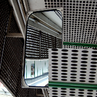
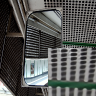
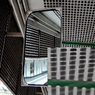
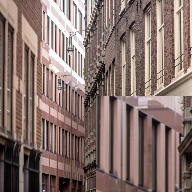
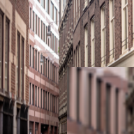
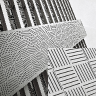
We also perform the visualization comparison to show the effectiveness of structural information restoration and aliasing suppression. Figure 11 shows the example aliasing images in Urban100. We can find the aliasing is heavy in LR instances. Compared with other methods, our network can suppress the aliasing and restore the accurate textures more effectively. This is because the buildings contain abundant repeated information, and the adjacent patches usually holds similar textures. In this point of view, local image prior can provide a good guidance for image restoration. For the first row in the figure, the textures of the holes are similar, and our network can distinguish more accurate circles under the aliasing. For the last row in the figure, the lines are similar, and we can recover more correct lines.

(a) HR(PSNR/SSIM)

(b) LR(28.50/0.7866)

(c) VDSR [4](30.22/0.8242)

(d) CrossSRN [52](30.77/0.8349)

(e) MSRN [12](30.66/0.8337)

(f) HSRNet(30.90/0.8375)

(g) HR(PSNR/SSIM)

(h) LR(23.10/0.6901)

(i) VDSR [4](25.47/0.7665)

(j) CrossSRN [52](26.30/0.7842)

(k) MSRN [12](26.19/0.7842)

(l) HSRNet(26.41/0.7860)

Figure 12: Visualization comparisons on Set14 with BI $\times 4$.

(a) HR(PSNR/SSIM)

(b) LR(27.51/0.8346)

(c) VDSR [4](28.37/0.8684)

(d) CrossSRN [52](28.50/0.8757)

(e) MSRN [12](29.13/0.8790)

(f) HSRNet(29.88/0.8818)

(g) HR(PSNR/SSIM)

(h) LR(26.15/0.7523)

(i) VDSR [4](27.73/0.8077)

(j) CrossSRN [52](28.23/0.8222)

(k) MSRN [12](28.01/0.8197)

(l) HSRNet(28.23/0.8224)

Figure 13: Visualization comparisons on B100 with BI $\times 4$.

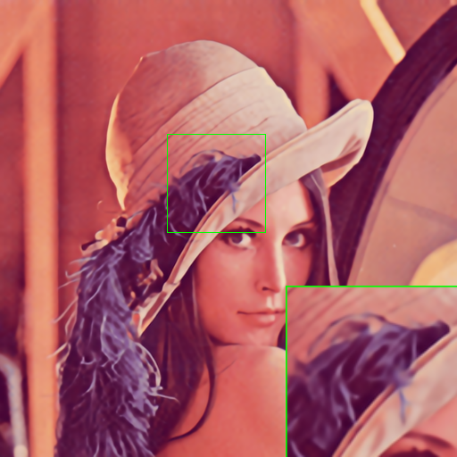
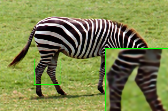
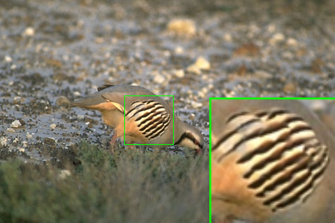
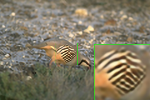
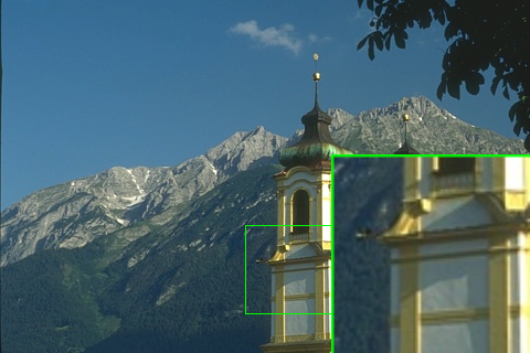
To demonstrate the effectiveness on different objects and scenarios, we compare our method with different methods on big and small animals, people and building from Set14 [38] and B100 [39] benchmarks, which contains the natural and the man-made scenarios. Figure 12 and 13 shows the visualization comparisons. In Figure 12, the hairs are mixed by the bicubic degradation. HSRNet restores more accurate edges than other works. The zebra’s leg suffers from aliasing effect which makes it hard to restore the correct textures. Compared with other works, the result of HSRNet is closest to the HR image. Figure 13 also demonstrates the effectiveness of our method in the natural scenario. We can find that the wing of the bird is highly mixed by the degradation. HSRNet can suppress the aliasing effect and restore better textures than other works. Similarly, the lines of the building can be better reconstructed by our HSRNet. In this point of view, HSRNet is effective on different objects and scenarios.

IV-D Discussion

Figure 14: Comparison between the local self-similarity and the restoration performance. The values denote the PSNR/SSIM/LSS results of the image. (a) row shows the images with lower LSS and (b) row shows the images with higher LSS.

TABLE VII: Investigation on the PLCC/SRCC results between PSNR and LSS on different benchmarks with $\textbf{BI}\times 4$.

Images	Set14	B100	Urban100	Manga109
LR	0.4423/0.3670	0.4807/0.4571	0.6124/0.5961	0.5905/0.5433
SR	0.6337/0.5824	0.7620/0.8039	0.7130/0.7259	0.8084/0.7651
HR	0.8553/0.7758	0.9149/0.9326	0.8205/0.8447	0.8719/0.8506

The local self-similarity (LSS) is the key point for HSRNet to restore the HR image. To model the local self-similarity, we learn from the conception of self-similarity descriptor [53] and propose a method to estimate the similarity of the image. For an image pixel $ip$, we compare the surrounding patch $p_{lss}$ with size $5\times 5$ and a larger surrounding region $r_{lss}$ with size $40\times 40$. We convert the $p_{lss}$ and $r_{lss}$ into Lab color space and calculate the sum of square difference (SSD) in L channel. The result $SSD(p_{lss},r_{lss})$ contains $8\times 8$ values, denoting the differences between $p_{lss}$ and patches in $r_{lss}$ without overlap. Then, the local self-similarity of image pixel $ip$ is estimated by

$$LSS(ip)=\max(\exp(-SSD(p_{lss},r_{lss}))).$$ (20)

The $SSD(p_{lss},r_{lss})$ describes the difference between the central patch and its neighbors. When $SSD(p_{lss},r_{lss})$ is smaller, $LSS(ip)$ becomes larger and there is higher local self-similarity surrounding image pixel $ip$. As such, $LSS(\cdot)$ is a feasible descriptor for the local self-similarity.

The local self-similarity of the image is estimated as follows. Firstly, we separate the image into several $40\times 40$ patches without overlap. Then, we calculate the LSS for every patch. The average of LSS is regarded as the local self-similarity of the image.

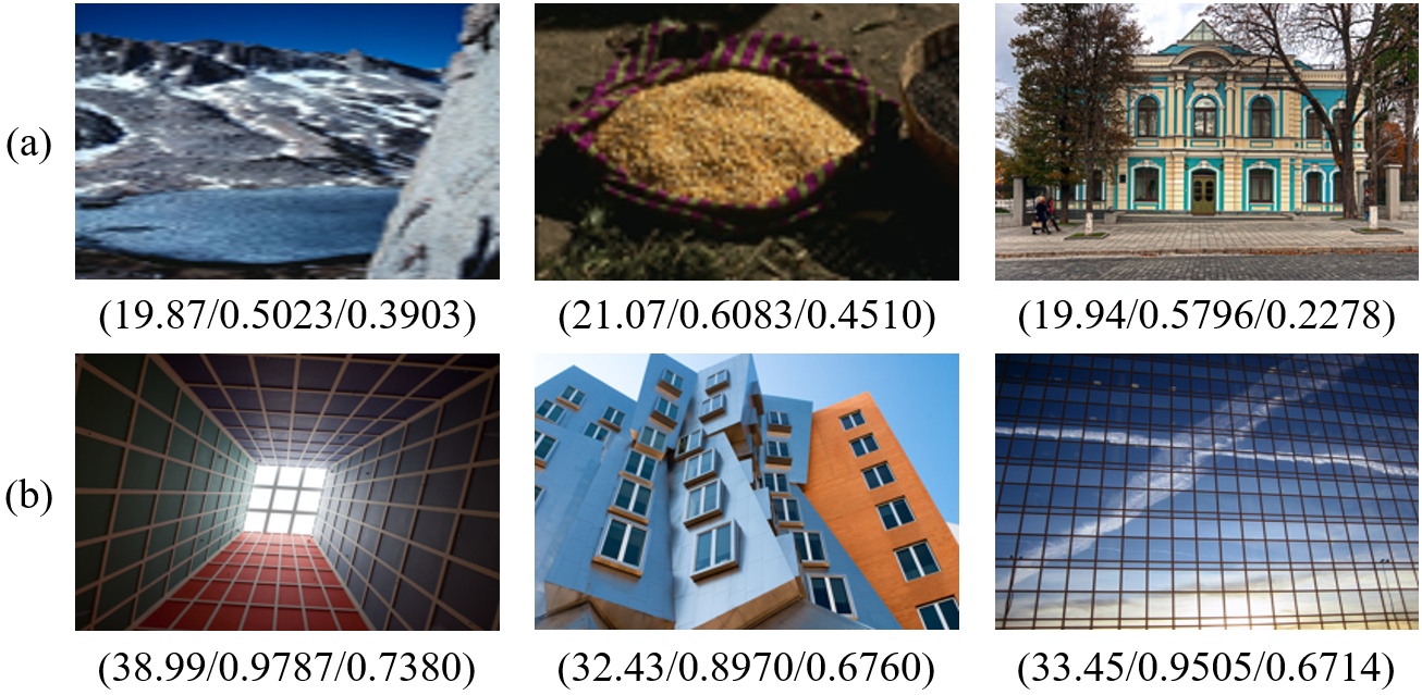
In general, the images contain fewer high-frequency details and more clear structural textures are with higher local self-similarity and more suitable for HSRNet to restore. Figure 14 shows the comparison between the local self-similarity and the restoration performance. The values under the image denote the PSNR/SSIM/LSS results. (a) row of the figure shows the images with lower LSS and (b) row shows the images with higher LSS. We can find that images in Figure 14 (a) contain more high-frequency details and tiny textures, which cause lower LSS values. The PSNR/SSIM results of these images are still lower. In contrast to the (a) row, images in Figure 14 (b) have more clear structural textures and fewer high-frequency details. In this point of view, the PSNR/SSIM results of the images are much higher with larger LSS values.

From the perspective a user, LSS can be a good criterion to judge whether the image should be restored by HSRNet. The image with higher LSS value usually can be well reconstructed with higher PSNR results. To address this point, we calculate the Pearson’s linear correlation coefficient (PLCC) and the Spearman’s rank correlation coefficient (SRCC) to show the consistency between LSS and PSNR. Table VII shows the PLCC/SRCC results between PSNR and LSS on different benchmarks with $\textbf{BI}\times 4$. We can find that the correlation coefficients of HR and SR images are higher than 0.5 on all benchmarks. The higher PLCC/SRCC results denote higher correlations between LSS and PSNR. It should be noted that the correlations of LR are lower than SR and HR. This is because there is aliasing effect in the LR images, causing the mixture of textures and decrease the LSS. Even though, the PLCC/SRCC results of Urban100 and Manga109 are still higher than 0.5. HSRNet suppress the aliasing effect in SR images, and improves the PLCC/SRCC results. In this point of view, the user can calculate the LSS after HSRNet as a posterior. If the LSS is higher, then the restored image usually holds a better objective quality.

V Conclusion

In this paper, we proposed a hierarchical similarity learning network for aliasing suppressing image super-resolution, which is termed as HSRNet. We found there are correlations and self-similarities among the adjacent patches in the natural images, and devised the hierarchical exploration blocks (HEBs) to learn the local image prior. To obtain the relations of adjacent feature and focus more on the high-frequency information, multi-level spatial attention (MSA) was proposed to boost the restoration performance. Furthermore, we considered the issue in the optimization perspective and proposed a hierarchical similarity learning super-resolution network (HSRNet) based on the half-quadratic splitting strategy. Experimental results show our HSRNet achieves better performance than other works. When compared with other iterative works, HSRNet achieves competitive or better performance with much fewer parameters and lower computation complexity. Furthermore, the visualization comparisons show HSRNet can suppress the aliasing and restore the correct textures more effectively than other works.

References

- [1] Z. Wang, J. Chen, and S. C. Hoi, “Deep learning for image super-resolution: A survey,” IEEE Transactions on Pattern Analysis and Machine Intelligence (TPAMI), pp. 1–1, 2020.
- [2] T. Blumensath and M. E. Davies, “Sampling theorems for signals from the union of finite-dimensional linear subspaces,” IEEE Transactions on Information Theory (TIT), vol. 55, no. 4, pp. 1872–1882, 2009.
- [3] C. Dong, C. C. Loy, K. He, and X. Tang, “Image super-resolution using deep convolutional networks,” IEEE Transactions on Pattern Analysis and Machine Intelligence (TPAMI), vol. 38, no. 2, pp. 295–307, 2016.
- [4] J. Kim, J. K. Lee, and K. M. Lee, “Accurate image super-resolution using very deep convolutional networks,” in IEEE Conference on Computer Vision and Pattern Recognition (CVPR), 2016, pp. 1646–1654.
- [5] B. Lim, S. Son, H. Kim, S. Nah, and K. M. Lee, “Enhanced deep residual networks for single image super-resolution,” in IEEE Conference on Computer Vision and Pattern Recognition Workshops (CVPRW), 2017, pp. 1132–1140.
- [6] W.-S. Lai, J.-B. Huang, N. Ahuja, and M.-H. Yang, “Fast and accurate image super-resolution with deep laplacian pyramid networks,” IEEE Transactions on Pattern Analysis and Machine Intelligence (TPAMI), vol. 41, no. 11, pp. 2599–2613, 2019.
- [7] H. Yue, X. Sun, J. Yang, and F. Wu, “Landmark image super-resolution by retrieving web images,” IEEE Transactions on Image Processing (TIP), vol. 22, no. 12, pp. 4865–4878, 2013.
- [8] R. Timofte, V. De, and L. V. Gool, “Anchored neighborhood regression for fast example-based super-resolution,” in IEEE International Conference on Computer Vision (ICCV), 2013, pp. 1920–1927.
- [9] J. Liu, W. Yang, X. Zhang, and Z. Guo, “Retrieval compensated group structured sparsity for image super-resolution,” IEEE Transactions on Multimedia (TMM), vol. 19, no. 2, pp. 302–316, 2017.
- [10] H. Zheng, M. Ji, H. Wang, Y. Liu, and L. Fang, “Crossnet: An end-to-end reference-based super resolution network using cross-scale warping,” in European Conference on Computer Vision (ECCV), vol. 11210, 2018, pp. 87–104.
- [11] Z. Zhang, Z. Wang, Z. Lin, and H. Qi, “Image super-resolution by neural texture transfer,” in IEEE/CVF Conference on Computer Vision and Pattern Recognition (CVPR), 2019, pp. 7974–7983.
- [12] J. Li, F. Fang, K. Mei, and G. Zhang, “Multi-scale residual network for image super-resolution,” in European Conference on Computer Vision (ECCV), 2018, pp. 527–542.
- [13] J. Huang, A. Singh, and N. Ahuja, “Single image super-resolution from transformed self-exemplars,” in IEEE Conference on Computer Vision and Pattern Recognition (CVPR), 2015, pp. 5197–5206.
- [14] W. Shi, J. Caballero, F. Huszár, J. Totz, A. P. Aitken, R. Bishop, D. Rueckert, and Z. Wang, “Real-time single image and video super-resolution using an efficient sub-pixel convolutional neural network,” in IEEE Conference on Computer Vision and Pattern Recognition (CVPR), 2016, pp. 1874–1883.
- [15] T. Tong, G. Li, X. Liu, and Q. Gao, “Image super-resolution using dense skip connections,” in IEEE International Conference on Computer Vision (ICCV), 2017, pp. 4809–4817.
- [16] Y. Zhang, Y. Tian, Y. Kong, B. Zhong, and Y. Fu, “Residual dense network for image super-resolution,” in IEEE/CVF Conference on Computer Vision and Pattern Recognition (CVPR), 2018, pp. 2472–2481.
- [17] Y. Zhang, K. Li, K. Li, L. Wang, B. Zhong, and Y. Fu, “Image super-resolution using very deep residual channel attention networks,” in European Conference on Computer Vision (ECCV), 2018, pp. 294–310.
- [18] X. He, Z. Mo, P. Wang, Y. Liu, M. Yang, and J. Cheng, “Ode-inspired network design for single image super-resolution,” in IEEE/CVF Conference on Computer Vision and Pattern Recognition (CVPR), 2019, pp. 1732–1741.
- [19] M. Haris, G. Shakhnarovich, and N. Ukita, “Deep back-projection networks for single image super-resolution,” IEEE Transactions on Pattern Analysis and Machine Intelligence (TPAMI), pp. 1–1, 2020.
- [20] Z. Li, J. Yang, Z. Liu, X. Yang, G. Jeon, and W. Wu, “Feedback network for image super-resolution,” in IEEE/CVF Conference on Computer Vision and Pattern Recognition (CVPR), 2019, pp. 3862–3871.
- [21] Y. Guo, J. Chen, J. Wang, Q. Chen, J. Cao, Z. Deng, Y. Xu, and M. Tan, “Closed-loop matters: Dual regression networks for single image super-resolution,” in IEEE/CVF Conference on Computer Vision and Pattern Recognition (CVPR), 2020, pp. 5406–5415.
- [22] Y. Mei, Y. Fan, Y. Zhou, L. Huang, T. S. Huang, and H. Shi, “Image super-resolution with cross-scale non-local attention and exhaustive self-exemplars mining,” in IEEE/CVF Conference on Computer Vision and Pattern Recognition (CVPR), 2020, pp. 5689–5698.
- [23] N. Ahn, B. Kang, and K. Sohn, “Fast, accurate, and lightweight super-resolution with cascading residual network,” in European Conference on Computer Vision (ECCV), 2018, pp. 256–272.
- [24] Z. Hui, X. Wang, and X. Gao, “Fast and accurate single image super-resolution via information distillation network,” in IEEE/CVF Conference on Computer Vision and Pattern Recognition (CVPR), 2018, pp. 723–731.
- [25] Z. Hui, X. Gao, Y. Yang, and X. Wang, “Lightweight image super-resolution with information multi-distillation network,” in ACM International Conference on Multimedia (MM), 2019, p. 2024–2032.
- [26] K. Zhang, M. Danelljan, Y. Li, and et. al., “AIM 2020 challenge on efficient super-resolution: Methods and results,” in European Conference on Computer Vision Workshops (ECCVW), 2020, pp. 5–40.
- [27] J. Hu, L. Shen, and G. Sun, “Squeeze-and-excitation networks,” in IEEE/CVF Conference on Computer Vision and Pattern Recognition (CVPR), 2018, pp. 7132–7141.
- [28] K. Zhang, W. Zuo, S. Gu, and L. Zhang, “Learning deep cnn denoiser prior for image restoration,” in IEEE Conference on Computer Vision and Pattern Recognition (CVPR), 2017, pp. 2808–2817.
- [29] K. Zhang, W. Zuo, and L. Zhang, “Deep plug-and-play super-resolution for arbitrary blur kernels,” in IEEE/CVF Conference on Computer Vision and Pattern Recognition (CVPR), 2019, pp. 1671–1681.
- [30] K. Zhang, L. Van Gool, and R. Timofte, “Deep unfolding network for image super-resolution,” in IEEE/CVF Conference on Computer Vision and Pattern Recognition (CVPR), 2020, pp. 3214–3223.
- [31] Y. Liu, S. Wang, J. Zhang, S. Wang, S. Ma, and W. Gao, “Iterative network for image super-resolution,” IEEE Transactions on Multimedia, pp. 1–1, 2021.
- [32] S. H. Chan, X. Wang, and O. A. Elgendy, “Plug-and-play admm for image restoration: Fixed-point convergence and applications,” IEEE Transactions on Computational Imaging (TCI), vol. 3, no. 1, pp. 84–98, 2017.
- [33] X. Deng and P. L. Dragotti, “Deep coupled ista network for multi-modal image super-resolution,” IEEE Transactions on Image Processing (TIP), vol. 29, pp. 1683–1698, 2020.
- [34] J. Zhang and B. Ghanem, “Ista-net: Interpretable optimization-inspired deep network for image compressive sensing,” in IEEE/CVF Conference on Computer Vision and Pattern Recognition (CVPR), 2018, pp. 1828–1837.
- [35] J. Ma, X.-Y. Liu, Z. Shou, and X. Yuan, “Deep tensor admm-net for snapshot compressive imaging,” in 2019 IEEE/CVF International Conference on Computer Vision (ICCV), 2019, pp. 10 222–10 231.
- [36] E. Agustsson and R. Timofte, “Ntire 2017 challenge on single image super-resolution: Dataset and study,” in IEEE Conference on Computer Vision and Pattern Recognition Workshops (CVPRW), 2017, pp. 1122–1131.
- [37] M. Bevilacqua, A. Roumy, C. Guillemot, and M. line Alberi Morel, “Low-complexity single-image super-resolution based on nonnegative neighbor embedding,” in British Machine Vision Conference (BMVC), 2012, pp. 135.1–135.10.
- [38] R. Zeyde, M. Elad, and M. Protter, “On single image scale-up using sparse-representations,” in International Conference on Curves and Surfaces. Springer, 2010, pp. 711–730.
- [39] D. Martin, C. Fowlkes, D. Tal, and J. Malik, “A database of human segmented natural images and its application to evaluating segmentation algorithms and measuring ecological statistics,” in IEEE International Conference on Computer Vision (ICCV), vol. 2, 2001, pp. 416–423 vol.2.
- [40] Y. Matsui, K. Ito, Y. Aramaki, A. Fujimoto, T. Ogawa, T. Yamasaki, and K. Aizawa, “Sketch-based manga retrieval using manga109 dataset,” Multimedia Tools and Applications (MTA), vol. 76, no. 20, pp. 21 811–21 838, 2017.
- [41] C. Dong, C. C. Loy, and X. Tang, “Accelerating the super-resolution convolutional neural network,” in European Conference on Computer Vision (ECCV), 2016, pp. 391–407.
- [42] J. Kim, J. K. Lee, and K. M. Lee, “Deeply-recursive convolutional network for image super-resolution,” in IEEE Conference on Computer Vision and Pattern Recognition (CVPR), 2016, pp. 1637–1645.
- [43] Y. Tai, J. Yang, and X. Liu, “Image super-resolution via deep recursive residual network,” in IEEE Conference on Computer Vision and Pattern Recognition (CVPR), 2017, pp. 2790–2798.
- [44] Y. Tai, J. Yang, X. Liu, and C. Xu, “Memnet: A persistent memory network for image restoration,” in IEEE International Conference on Computer Vision (ICCV), 2017, pp. 4549–4557.
- [45] W. Yang, J. Feng, J. Yang, F. Zhao, J. Liu, Z. Guo, and S. Yan, “Deep edge guided recurrent residual learning for image super-resolution,” IEEE Transactions on Image Processing, vol. 26, no. 12, pp. 5895–5907, 2017.
- [46] Y. Wang, L. Wang, H. Wang, and P. Li, “Resolution-aware network for image super-resolution,” IEEE Transactions on Circuits and Systems for Video Technology, vol. 29, no. 5, pp. 1259–1269, 2019.
- [47] C. Xie, W. Zeng, and X. Lu, “Fast single-image super-resolution via deep network with component learning,” IEEE Transactions on Circuits and Systems for Video Technology, vol. 29, no. 12, pp. 3473–3486, 2019.
- [48] F. Li, H. Bai, and Y. Zhao, “Filternet: Adaptive information filtering network for accurate and fast image super-resolution,” IEEE Transactions on Circuits and Systems for Video Technology, vol. 30, no. 6, pp. 1511–1523, 2020.
- [49] Z. He, Y. Cao, L. Du, B. Xu, J. Yang, Y. Cao, S. Tang, and Y. Zhuang, “MRFN: multi-receptive-field network for fast and accurate single image super-resolution,” IEEE Transactions on Multimedia, vol. 22, no. 4, pp. 1042–1054, 2020.
- [50] F. Fang, J. Li, and T. Zeng, “Soft-edge assisted network for single image super-resolution,” IEEE Transactions on Image Processing, vol. 29, pp. 4656–4668, 2020.
- [51] B. Li, B. Wang, J. Liu, Z. Qi, and Y. Shi, “s-lwsr: Super lightweight super-resolution network,” IEEE Transactions on Image Processing (TIP), vol. 29, pp. 8368–8380, 2020.
- [52] Y. Liu, Q. Jia, X. Fan, S. Wang, S. Ma, and W. Gao, “Cross-srn: Structure-preserving super-resolution network with cross convolution,” IEEE Transactions on Circuits and Systems for Video Technology, pp. 1–1, 2021.
- [53] E. Shechtman and M. Irani, “Matching local self-similarities across images and videos,” in IEEE Conference on Computer Vision and Pattern Recognition (CVPR), 2007, pp. 1–8.