Classification of Pulsar Glitch Amplitudes using Extreme Deconvolution

Abstract

We carry out a classification of the glitch amplitudes of radio pulsars using Extreme Deconvolution technique based on the Gaussian Mixture Model, where the observed uncertainties in the glitch amplitudes $\left(\frac{\Delta\nu}{\nu}\right)$are taken into account. Our dataset consists of 699 glitches from 238 pulsars. We then use information theory criteria such as AIC and BIC to determine the optimum number of glitch classes. We find that both AIC and BIC show that the pulsar glitch amplitudes can be optimally described using a bimodal distribution. The mean values of $\left(\frac{\Delta\nu}{\nu}\right)$for the two components are equal to $4.79\times 10^{-9}$ and $1.28\times 10^{-6}$, respectively with standard deviation given by 1.01 and 0.55 dex. We also applied this method to classify the pulsar inter-glitch time intervals, and we find that AIC prefers two components, whereas BIC prefers a single component. The unified data set and analyses codes used in this work have been made publicly available.

I Introduction

Pulsars are rapidly rotating neutron stars which emit pulsed radio emission Kaspi and Kramer (2016). Although the periods of most pulsars are stable, a small fraction of young pulsars show abrupt discontinuities in their period. Glitches constitute one such discontinuity, where there is a sudden abrupt increase in the rotational frequency, with frequency jumps ranging from $(10^{-4}-10^{2})\mu$ Hz Espinoza et al. (2011); Manchester (2018). The glitch is followed by a recovery stage in which the rotation frequency asymptotes to the pre-glitch behaviour. The glitch amplitude is usually parameterized by $\left(\frac{\Delta\nu}{\nu}\right)$, where $\Delta\nu$ is the change in rotational frequency and $\nu$ is the observed frequency. This amplitude ranges from $10^{-11}-10^{-4}$, whereas the inter-glitch time interval varies between 20-1000 days Eya et al. (2019). Ever since the detection of the first glitch in the Vela pulsar in 1969 Radhakrishnan and Manchester (1969); Reichley and Downs (1969), glitches have proved to be a wonderful laboratory for probing the physics of the neutron star, in particular the nature of superfluid in the interior of the neutron star Baym et al. (1969). However, the full details of the glitch mechanisms are still not completely understood Haskell and Melatos (2015). Therefore, there are large number of observational campaigns on current as well as future radio telescopes to get more insights into the nature of glitches and their causes Singha et al. (2021). The study of pulsar glitches will also be one of the flagship science goals carried out during the SKA era Singha et al. (2022). Such glitches have also been observed in millisecond pulsars Cognard and Backer (2004); McKee et al. (2016) and also magnetars Dib and Kaspi (2014), where anti-glitches (corresponding to spin-down in the neutron star period) have been detected Archibald et al. (2013).

The study of pulsar glitches is very important for gravitational wave astronomy. Pulsar glitches could result in a gravitational wave burst van Eysden and Melatos (2008). Studying the statistical characteristics of these glitches is therefore important for designing search pipelines to look for such gravitational wave bursts Clark et al. (2007); Hayama et al. (2008); Prix et al. (2011). Furthermore, glitches could also affect the sensitivity of continuous gravitational wave (CW) searches Ashton et al. (2017). It is important to understand the probability of occurrence of a glitch during a CW and the impact of a probable glitch on its detectability. The statistical characteristics of the observed glitch population has also been used to extrapolate the glitch magnitudes for the unobserved neutron star population to understand its implications for CW searches Ashton et al. (2017).

There have been several studies which have looked at the statistical distribution of glitch amplitudes, which have alluded to a bimodal distribution Lyne et al. (2000); Wang et al. (2000); Espinoza et al. (2011); Yu et al. (2013); Fuentes et al. (2017); Konar and Arjunwadkar (2014); Ashton et al. (2017); Eya et al. (2017, 2019); Basu et al. (2022). A few works have previously carried out a GMM based analysis of the glitch amplitudes Ashton et al. (2017); Fuentes et al. (2017) or the fractional glitch amplitude Konar and Arjunwadkar (2014), followed by Bayesian Ashton et al. (2017) or AIC based model comparison test Fuentes et al. (2017). However none of these works have included the associated errors in the fractional glitch amplitudes. In addition to the aforementioned importance of understanding the statistical nature of glitches for gravitational wave astronomy, the bimodal nature of the glitch amplitude distribution is important for constructing unified models of the glitch phenomenon Celora et al. (2020). Therefore it is important to re-assess the robustness of the claim of bimodality of the glitch amplitude distribution, when the uncertainties are incorporated, which hitherto has never been done.

For this purpose, we carry out a clustering based analysis of pulsar glitch amplitudes by applying the Extreme Deconvolution technique based on the Gaussian Mixture model Bovy et al. (2011) and determine the optimum number of classes using information theoretical criteria Krishak and Desai (2020a). This work follows up on our previous studies, where we applied these same techniques for the classification of pulsars (using their period and period derivatives)  Reddy Ch. and Desai (2022) and Gamma-Ray Bursts (using durations and hardness) Bhave et al. (2022).

This manuscript is structured as follows. The data set used for our analysis is described in Sect. II. The analysis methodology is described in Sect. III. Our results are discussed in Sect. IV and we conclude in Sect. V.

II Data Set

A complete catalog of pulsar glitches has been independently collated in two different locations: one at Jodrell Bank (JBO)  Espinoza et al. (2011) and also by ATNF Manchester et al. (2005). The JBO catalog contains 664 glitches from 207 distinct pulsars. Each JBO glitch entry consists of pulsar name, glitch MJD, glitch amplitude and its error, the first derivative of the glitch amplitude along with its error. In this catalog, two glitches did not have any associated amplitude and error, whereas 16 glitches had no associated uncertainties for $\left(\frac{\Delta\nu}{\nu}\right)$. The ATNF catalog contains 641 glitches from 211 distinct pulsars and 18 glitches without any associated pulsar. This catalog also contains 54 entries from 32 distinct pulsars, which are not in the JBO catalog.

For our analysis we primarily used the JBO catalogue. However, we appended to this catalog the 54 entries from the ATNF list which were absent from JBO. We also checked to see if any of the entries with missing amplitude or error in the JBO catalog had corresponding values in the ATNF and we found 5 such events. After combining data from both the catalogs we had a total of 717 glitches from 238 distinct pulsars. After preprocessing the data to remove pulsars associated with negative glitch amplitude and ones with no associated uncertainties, we had a total of 699 glitches from 238 pulsars. The median value of the fractional error in the glitch amplitude is about 1.5%. The full dataset used for our analysis can be found at https://github.com/swetha9730/XDGMM-for-Pulsar-Glitches-Classification. Given the large dynamic range in $\left(\frac{\Delta\nu}{\nu}\right)$, we do the classification in logarithmic space using the base 10. We now describe the methodology used for classification.

III Methodology

III.1 XDGMM

Extreme Deconvolution (XDGMM) is a generalization of Gaussian Mixture Model (Kuhn and Feigelson, 2017) (GMM), which incorporates the uncertainty in the observed data Bovy et al. (2011); Ivezić et al. (2014); Holoien et al. (2017). It has been used for a variety of astrophysical applications, including determining the velocity distribution from Hipparcos Bovy et al. (2011), classification of pulsars Reddy Ch. and Desai (2022) and GRBs Bhave et al. (2022), the three-dimensional motions of Sagittarius stream stars  (Koposov et al., 2013), bifurcation of neutron star masses (Keitel, 2019), detection of dark matter subhalo candidates (Coronado-Blázquez et al., 2019). We provide a brief description of the XDGMM method, and use the same notation as  Reddy Ch. and Desai (2022); Bhave et al. (2022). More details about XDGMM can be found in  Bovy et al. (2011); Ivezić et al. (2014); Holoien et al. (2017). We note that GMM has also been extended to account for incomplete/missing as well as truncated data Melchior and Goulding (2018).

Consider a noisy data set $x_{i}$, which is related to the true values $v_{i}$ according to (Bovy et al., 2011; Ivezić et al., 2014):

$$x_{i}=R_{i}v_{i}+\epsilon_{i},$$ (1)

where $R_{i}$ is the rotation matrix used to transform the correct values to the observed noisy dataset. Similar to ordinary GMM, we assume that the probability density of the true values $v$ can be written as a mixture of $K$ Gaussians given by

$$p(v_{i})=\sum_{j=1}^{K}\alpha_{j}\mathcal{N}(v_{i}|\mu_{j},\Sigma_{j})$$ (2)

where $\mu_{j}$ and $\Sigma_{j}$ are the means and variances of each of the Gaussian distribution, and $\alpha_{j}$ is the weight of each Gaussian, subject to the constraint $\sum\limits_{j=1}^{K}\alpha_{j}=1$. For the example in this work, $x_{i}$ and $v_{i}$ represent the one-dimensional dataset given by $\log$ $\left(\frac{\Delta\nu}{\nu}\right)$. We assume that the noise $\epsilon_{i}$ (in Eq. 1) is a Gaussian random variable with zero mean and variance equal to $S_{i}$. The likelihood of the model parameters ($\theta\equiv$ {$\alpha$, $\mu$, $\Sigma$, $R_{i}$, $S_{i}$}) for each noisy data point ($x_{i}$) is then given by (Bovy et al., 2011):

$$p(x_{i}|\theta)=\sum_{j=1}^{K}\alpha_{j}\mathcal{N}(x_{i}|R_{i}\mu_{j},R_{i}\Sigma_{j}R_{i}^{T}+S_{i})$$ (3)

The final step in XDGMM is to maximize the likelihood of the dataset with respect to the model parameters. This can be done by summing the individual log-likelihood functions:

$$\underset{\theta}{\operatorname{argmax}}\;L=\sum_{i=1}^{N}\ln(p(x_{i}|\theta)),$$ (4)

where $N$ is the total number of data points. This objective function is maximized using an extension of the Expectation-maximization algorithm (Bovy et al., 2011). The output of XDGMM returns a likelihood, which can then be used for model selection.

III.2 Model Selection

There are basically three kinds of techniques used in literature to arbitrate between two models which are used to fit the data: frequentist, Bayesian, and information theoretical ones. More details on these techniques, including pitfalls and advantages of each of them can be found in  Liddle (2004); Kerscher and Weller (2019); Sharma (2017) or in some of our past works Kulkarni and Desai (2017, 2018); Ganguly and Desai (2017); Krishak et al. (2020); Krishak and Desai (2019); Singirikonda and Desai (2020); Krishak and Desai (2020b); Krishak and Desai (2020a). In this work, we shall use information theoretical techniques such as AIC and BIC, since they are straightforward to compute from the likelihood returned by XDGMM. We now add each of them below:

• AIC AIC is defined by

  $$AIC=2p-2\ln L_{max}.$$ (5)

  where $p$ is the number of free parameters in the model and $L_{max}$ is the maximum likelihood. For our analysis, $L_{max}$ is obtained from XDGMM. The model with the smaller value of AIC is considered as the better model and the significance can be assessed using the qualitative strength of evidence rules Krishak and Desai (2020a).

• BIC

  $$BIC=p\ln N-2\ln L_{max}.$$ (6)

  where $N$ is the number of data points and all the other terms is the same as in Eq. 5. BIC penalizes models with additional free parameters more harshly than AIC. Similar to AIC, the model with the smaller value of BIC is considered as the favored model and the significance can be assessed using the strength of evidence rules proposed for BIC Krishak and Desai (2020a).

III.3 XDGMM Implementation

We now apply XDGMM to our unified glitch catalog using $\log$ $\left(\frac{\Delta\nu}{\nu}\right)$as inputs, where $\log$ refers to logarithm to the base 10. The error in this quantity is given by $\frac{\sigma}{2.3\Delta\nu/\nu}$, where $\sigma$ refers to the uncertainty in $\left(\frac{\Delta\nu}{\nu}\right)$. We did not consider the data points for which $\left(\frac{\Delta\nu}{\nu}\right)$$<0$, since we are doing the fit in logarithmic space. We use the XDGMM implementation in the XDGMM classe (Holoien et al., 2017), which is a wrapper to the astroML module. The output of XDGMM consists of the weights, means, and covariances for the input number of clusters. In order to determine the optimum number of components, we apply XDGMM by varying the number of glitch classes from one to four and then use AIC/BIC to determine the best number among these.

IV Results

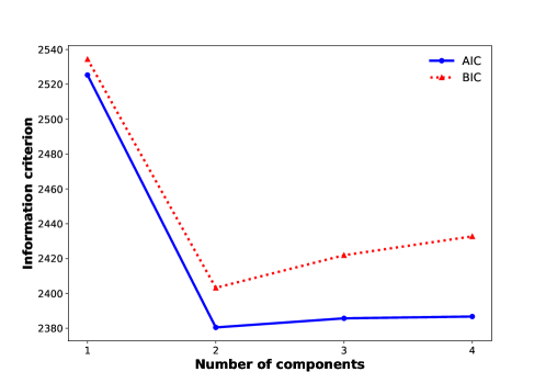
The AIC/BIC as a function of the number of glitch classes can be found in Fig. 1. Both AIC and BIC show a minimum for two glitch classes. BIC rises sharply as we increase the number of components with ($\Delta$BIC $>10$). Therefore, based on strength of evidence rules Liddle (2004); Krishak and Desai (2020a), BIC decisively favors two classes over any other. AIC also shows a minimum for two components, although the difference with respect to the third component is less than 10 ($\Delta$AIC=5). This is because AIC is more liberal while fitting complicated models. Still both the techniques agree that the optimum number of glitch classes (based on glitch amplitude) is equal to two.

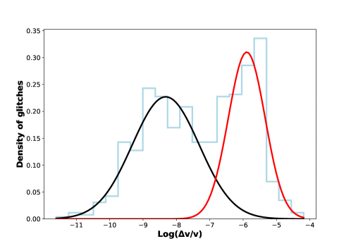
The mean value and standard deviation of the two components ($\mu,\sigma$) are given by (-8.32,1.01) and (-5.89,0.55) respectively. This corresponds to mean fractional glitch amplitude $\left(\frac{\Delta\nu}{\nu}\right)$equal to $4.79\times 10^{-9}$ and $1.28\times 10^{-6}$, respectively. There are 386 glitches which belong to the first component ($\mu_{1}=-8.32$) and 313 to the second component ($\mu_{2}=-5.89$). There are 98 glitches in the overlap region, where overlap region is defined by the region lying between $\mu_{1}+2\sigma_{1}$ and $\mu_{2}-2\sigma_{2}$.

Figure 1: AIC and BIC values as a function of the number of components. The minimum value of AIC/BIC is obtained for two components, indicating that the pulsar glitch amplitude can be adequately described using two classes.

Figure 2: Normalized histogram of the pulsar glitch amplitudes ($\log$ $\left(\frac{\Delta\nu}{\nu}\right)$) along with the Gaussian fit obtained using XDGMM. The mean value and standard deviation for the two components ($\mu,\sigma$) are given by (-8.32, 1.01) and (-5.89, 0.55) respectively.

IV.1 Application of XDGMM to inter-glitch arrival times

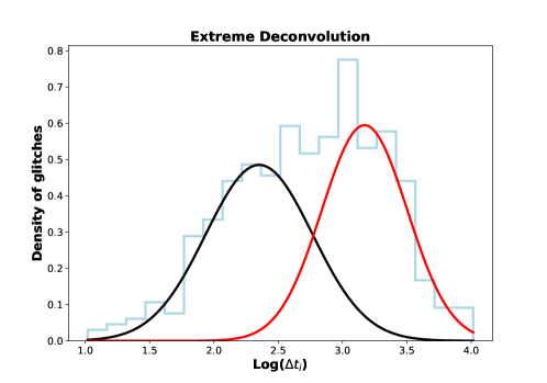
We now apply XDGMM to the pulsar inter-glitch arrival times, defined as the arrival time between multiple glitches for the same pulsars. The error in inter-glitch arrival times were obtained by adding in quadrature the uncertainty in both the time intervals. For this analysis, we used the same data-set used for XDGMM on fractional glitch amplitudes and further removed glitches which had no uncertainty in their MJD. We had a total of 658 glitches from 219 distinct pulsars and hence had 439 inter-glitch arrival times ($t_{i}$) (in days) after pre-processing the data. We again apply XDGMM for the glitch arrival times in logarithmic (to base 10) space.

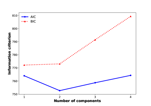
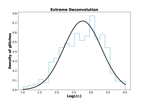
The results of XDGMM analysis can be found in Fig 3. The histogram of the inter-glitch arrival times along with the XDGMM best-fit for one component is shown in Fig. 4, and the same with two components in Fig. 5. We find that the BIC analysis points prefers an unimodal distribution, whereas the AIC analysis shows a preference for two components with $\Delta$ BIC (AIC) between the first and second component equal to -0.9 and 11.3, respectively. Therefore, AIC and BIC analyses lead to opposite conclusions. We have seen this previously also where AIC and BIC results did not always agree Kulkarni and Desai (2017, 2018); Bhave et al. (2022). We note that AIC and BIC answer different questions and are derived based on different assumptions. As emphasized by Tarnopolski Tarnopolski (2019), AIC chooses a model which describes reality for the data being analyzed, whereas BIC finds the correct model among the different hypotheses being tested. Therefore, they differ in how they penalize the number of free parameters, where BIC is more stringent in penalizing parameters with additional free parameters Tarnopolski (2019). Therefore BIC results are more trustworthy in case of a discrepancy, which is seen here. Therefore, the current data for inter-glitch time interval is consistent with an unimodal distribution.

Figure 3: AIC and BIC values as a function of the number of components. The minimum value of BIC is obtained for one components, while minimum value of AIC is obtained for two components.

Figure 4: Normalized histogram of the pulsar inter-glitch arrival time ($\log(\Delta t_{i})$)(in days) along with the Gaussian fit obtained using XDGMM. The mean value and standard deviation for the Gaussian fit ($\mu,\sigma$) are given by (2.76, 0.55).

Figure 5: Normalized histogram of the pulsar inter-glitch arrival time ($\log(\Delta t_{i})$)(in days) along with the Gaussian fit obtained using XDGMM assuming two components. The mean value and standard deviation for the two components ($\mu,\sigma$) are given by (2.35, 0.41) and (3.17, 0.33) respectively.

V Conclusions

In this work, we use an automated method to determine the optimum number of radio pulsar glitch classes using the fractional glitch amplitude. Although a large number of works have previously alluded to a bimodal distribution for the pulsar glitch amplitude, very few works have implemented model selection techniques to ascertain that two pulsar glitch components are decisively favored compared to other classes. Furthermore, no previous work has incorporated the observational uncertainties in their analysis.

To rectify this, we did a classification of $\left(\frac{\Delta\nu}{\nu}\right)$in logarithmic space, for all pulsar glitches collated in the JBO or ATNF catalog, using XDGMM which is an extension of the GMM technique, which incorporates the uncertainties in $\left(\frac{\Delta\nu}{\nu}\right)$. We used information theory criteria such as AIC and BIC to determine the optimum glitch classes. Our results for the variation of AIC and BIC as a function of the number of the components can be found in Fig. 1. We see that both AIC and BIC have a minimum value for two components. The difference in BIC for two components is greater than 10 compared to any other value. Therefore, BIC decisively favors two components. The difference between the AIC value for two and the next larger components is about five.

The dichotomy of the two glitch classes along with the XDGMM fit can be found in Fig. 2. The mean values of $\left(\frac{\Delta\nu}{\nu}\right)$for the two components are given by $4.78\times 10^{-9}$ and $1.38\times 10^{-6}$, respectively. Therefore our results for the classification of fractional glitch amplitude are consistent with previous works Lyne et al. (2000); Wang et al. (2000); Espinoza et al. (2011); Yu et al. (2013); Fuentes et al. (2017); Konar and Arjunwadkar (2014); Ashton et al. (2017); Eya et al. (2017, 2019); Basu et al. (2022), which also pointed to a bimodal distribution, even though these works did not consider the uncertainty in the glitch amplitudes.

We have also applied this method to inter-glitch arrival time. The AIC/BIC distribution for this can be found in Fig. 3. We find that BIC based analysis supports a single distribution, whereas AIC analysis prefers two components. The best-fit single and two component models for the inter-glitch intervals can be found in Fig. 4 and Fig. 5. In such a scenario, the BIC based analysis is more trustworthy Tarnopolski (2019).

Therefore, our results on the autonomous classification of glitches corroborate previous results in literature which alluded to two distinct classes. Since extensions to GMM can account for the observational uncertainties as well as incompleteness, it is very important to have an accurate characterization of not only all the glitch observables, but also their uncertainties, completeness and upper limits, as we head into the SKA era Singha et al. (2022). We should obtain lot more statistics for pulsar glitches during the SKA era and incorporating the uncertainties and completeness into the analyses, could alter our Physics inferences. We can also apply our current technique to other pulsar glitch observables such as glitch activity, absolute glitch amplitude, etc. In order to carry out a similar analysis on the glitch activity, we would need an accurate estimate of the total time interval over which each pulsar has been monitored. Unfortunately, this information is not publicly available at the time of writing. Once this has been made publicly available, we can apply the XDGMM technique for classification of the glitch activity.

The unified data set used for this analysis along with the codes have been uploaded at https://github.com/swetha9730/XDGMM-for-Pulsar-Glitches-Classification.

References

- Kaspi and Kramer (2016) V. M. Kaspi and M. Kramer, arXiv e-prints arXiv:1602.07738 (2016), eprint 1602.07738.
- Espinoza et al. (2011) C. M. Espinoza, A. G. Lyne, B. W. Stappers, and M. Kramer, Mon. Not. R. Astron. Soc. 414, 1679 (2011), eprint 1102.1743.
- Manchester (2018) R. N. Manchester, arXiv e-prints arXiv:1801.04332 (2018), eprint 1801.04332.
- Eya et al. (2019) I. O. Eya, J. O. Urama, and A. E. Chukwude, Research in Astronomy and Astrophysics 19, 089 (2019), eprint 1812.10053.
- Radhakrishnan and Manchester (1969) V. Radhakrishnan and R. N. Manchester, Nature (London) 222, 228 (1969).
- Reichley and Downs (1969) P. E. Reichley and G. S. Downs, Nature (London) 222, 229 (1969).
- Baym et al. (1969) G. Baym, C. Pethick, D. Pines, and M. Ruderman, Nature (London) 224, 872 (1969).
- Haskell and Melatos (2015) B. Haskell and A. Melatos, International Journal of Modern Physics D 24, 1530008 (2015), eprint 1502.07062.
- Singha et al. (2021) J. Singha, A. Basu, M. A. Krishnakumar, B. C. Joshi, and P. Arumugam, Mon. Not. R. Astron. Soc. 505, 5488 (2021), eprint 2106.01942.
- Singha et al. (2022) J. Singha, B. C. Joshi, D. Bandyopadhyay, H. Grover, S. Desai, P. Arumugam, and S. Banik, arXiv e-prints arXiv:2207.06446 (2022), eprint 2207.06446.
- Cognard and Backer (2004) I. Cognard and D. C. Backer, Astrophys. J. Lett. 612, L125 (2004), eprint astro-ph/0407546.
- McKee et al. (2016) J. W. McKee, G. H. Janssen, B. W. Stappers, A. G. Lyne, R. N. Caballero, L. Lentati, G. Desvignes, A. Jessner, C. A. Jordan, R. Karuppusamy, et al., Mon. Not. R. Astron. Soc. 461, 2809 (2016), eprint 1606.04098.
- Dib and Kaspi (2014) R. Dib and V. M. Kaspi, Astrophys. J. 784, 37 (2014), eprint 1401.3085.
- Archibald et al. (2013) R. F. Archibald, V. M. Kaspi, C. Y. Ng, K. N. Gourgouliatos, D. Tsang, P. Scholz, A. P. Beardmore, N. Gehrels, and J. A. Kennea, Nature (London) 497, 591 (2013), eprint 1305.6894.
- van Eysden and Melatos (2008) C. A. van Eysden and A. Melatos, Classical and Quantum Gravity 25, 225020 (2008), eprint 0809.4352.
- Clark et al. (2007) J. Clark, I. S. Heng, M. Pitkin, and G. Woan, Phys. Rev. D 76, 043003 (2007), eprint gr-qc/0703138.
- Hayama et al. (2008) K. Hayama, S. Desai, S. D. Mohanty, M. Rakhmanov, T. Summerscales, and S. Yoshida, Classical and Quantum Gravity 25, 184016 (2008), eprint 0807.3983.
- Prix et al. (2011) R. Prix, S. Giampanis, and C. Messenger, Phys. Rev. D 84, 023007 (2011), eprint 1104.1704.
- Ashton et al. (2017) G. Ashton, R. Prix, and D. I. Jones, Phys. Rev. D 96, 063004 (2017), eprint 1704.00742.
- Lyne et al. (2000) A. G. Lyne, S. L. Shemar, and F. G. Smith, Mon. Not. R. Astron. Soc. 315, 534 (2000).
- Wang et al. (2000) N. Wang, R. N. Manchester, R. T. Pace, M. Bailes, V. M. Kaspi, B. W. Stappers, and A. G. Lyne, Mon. Not. R. Astron. Soc. 317, 843 (2000), eprint astro-ph/0005561.
- Yu et al. (2013) M. Yu, R. N. Manchester, G. Hobbs, S. Johnston, V. M. Kaspi, M. Keith, A. G. Lyne, G. J. Qiao, V. Ravi, J. M. Sarkissian, et al., Mon. Not. R. Astron. Soc. 429, 688 (2013), eprint 1211.2035.
- Fuentes et al. (2017) J. R. Fuentes, C. M. Espinoza, A. Reisenegger, B. Shaw, B. W. Stappers, and A. G. Lyne, Astron. & Astrophys. 608, A131 (2017), eprint 1710.00952.
- Konar and Arjunwadkar (2014) S. Konar and M. Arjunwadkar, in Astronomical Society of India Conference Series (2014), vol. 13 of Astronomical Society of India Conference Series, pp. 87–88, eprint 1402.1594.
- Eya et al. (2017) I. O. Eya, J. O. Urama, and A. E. Chukwude, Astrophys. J. 840, 56 (2017).
- Basu et al. (2022) A. Basu, B. Shaw, D. Antonopoulou, M. J. Keith, A. G. Lyne, M. B. Mickaliger, B. W. Stappers, P. Weltevrede, and C. A. Jordan, Mon. Not. R. Astron. Soc. 510, 4049 (2022), eprint 2111.06835.
- Celora et al. (2020) T. Celora, V. Khomenko, M. Antonelli, and B. Haskell, Mon. Not. R. Astron. Soc. 496, 5564 (2020), eprint 2002.04310.
- Bovy et al. (2011) J. Bovy, D. W. Hogg, and S. T. Roweis, Annals of Applied Statistics 5, 1657 (2011), eprint 0905.2979.
- Krishak and Desai (2020a) A. Krishak and S. Desai, JCAP 2020, 006 (2020a), eprint 2003.10127.
- Reddy Ch. and Desai (2022) T. T. Reddy Ch. and S. Desai, New Astronomy 91, 101673 (2022), eprint 2011.03771.
- Bhave et al. (2022) A. Bhave, S. Kulkarni, S. Desai, and P. K. Srijith, Astrophys. and Space Science 367, 39 (2022), eprint 1708.05668.
- Manchester et al. (2005) R. N. Manchester, G. B. Hobbs, A. Teoh, and M. Hobbs, Astron. J. 129, 1993 (2005), eprint astro-ph/0412641.
- Kuhn and Feigelson (2017) M. A. Kuhn and E. D. Feigelson, ArXiv e-prints (2017), eprint 1711.11101.
- Ivezić et al. (2014) Ž. Ivezić, A. Connolly, J. Vanderplas, and A. Gray, Statistics, Data Mining and Machine Learning in Astronomy (Princeton University Press, 2014).
- Holoien et al. (2017) T. W. S. Holoien, P. J. Marshall, and R. H. Wechsler, Astron. J. 153, 249 (2017), eprint 1611.00363.
- Koposov et al. (2013) S. E. Koposov, V. Belokurov, and N. W. Evans, Astrophys. J. 766, 79 (2013), eprint 1301.7070.
- Keitel (2019) D. Keitel, Mon. Not. R. Astron. Soc. 485, 1665 (2019), eprint 1808.01129.
- Coronado-Blázquez et al. (2019) J. Coronado-Blázquez, M. A. Sánchez-Conde, M. Di Mauro, A. Aguirre-Santaella, I. Ciucă, A. Domínguez, D. Kawata, and N. Mirabal, JCAP 2019, 045 (2019), eprint 1910.14429.
- Melchior and Goulding (2018) P. Melchior and A. D. Goulding, Astronomy and Computing 25, 183 (2018), eprint 1611.05806.
- Liddle (2004) A. R. Liddle, Mon. Not. R. Astron. Soc. 351, L49 (2004), eprint astro-ph/0401198.
- Kerscher and Weller (2019) M. Kerscher and J. Weller, SciPost Physics Lecture Notes 9 (2019), eprint 1901.07726.
- Sharma (2017) S. Sharma, Ann. Rev. Astron. Astrophys. 55, 213 (2017), eprint 1706.01629.
- Kulkarni and Desai (2017) S. Kulkarni and S. Desai, Astrophys. and Space Science 362, 70 (2017), eprint 1612.08235.
- Kulkarni and Desai (2018) S. Kulkarni and S. Desai, The Open Journal of Astrophysics 1, 4 (2018), eprint 1708.00605.
- Ganguly and Desai (2017) S. Ganguly and S. Desai, Astroparticle Physics C94, 17 (2017), eprint 1706.01202.
- Krishak et al. (2020) A. Krishak, A. Dantuluri, and S. Desai, JCAP 2020, 007 (2020), eprint 1906.05726.
- Krishak and Desai (2019) A. Krishak and S. Desai, The Open Journal of Astrophysics 2, E12 (2019), eprint 1907.07199.
- Singirikonda and Desai (2020) H. Singirikonda and S. Desai, European Physical Journal C 80, 694 (2020), eprint 2003.00494.
- Krishak and Desai (2020b) A. Krishak and S. Desai, Progress of Theoretical and Experimental Physics 2020, 093F01 (2020b), eprint 1910.05096.
- Tarnopolski (2019) M. Tarnopolski, Astrophys. J. 870, 105 (2019), eprint 1811.06745.