Good Intentions:
Adaptive Parameter Management via Intent Signaling

Abstract.

Model parameter management is essential for distributed training of large machine learning (ML) tasks. Some ML tasks are hard to distribute because common approaches to parameter management can be highly inefficient. Advanced parameter management approaches—such as selective replication or dynamic parameter allocation—can improve efficiency, but they typically need to be integrated manually into each task’s implementation and they require expensive upfront experimentation to tune correctly. In this work, we explore whether these two problems can be avoided. We first propose a novel intent signaling mechanism that integrates naturally into existing ML stacks and provides the parameter manager with crucial information about parameter accesses. We then describe AdaPM, a fully adaptive, zero-tuning parameter manager based on this mechanism. In contrast to prior parameter managers, our approach decouples how access information is provided (simple) from how and when it is exploited (hard). In our experimental evaluation, AdaPM matched or outperformed state-of-the-art parameter managers out of the box, suggesting that automatic parameter management is possible.

1. Introduction

Distributed training is essential for large-scale machine learning (ML) tasks. It enables (i) training of models that exceed the memory capacity of a single node and (ii) faster training by leveraging the compute of multiple nodes of a cluster. Typically, each node accesses one (local) partition of the training data, but requires global read and write access to all model parameters. Thus, parameter management (PM) among nodes is a key concern in distributed training. We refer to any system that provides distributed PM, i.e., that provides global parameter access across a cluster, as parameter manager. Most ML systems include a parameter manager as core component (Abadi et al., 2016; Paszke et al., 2019; Chen et al., 2015).

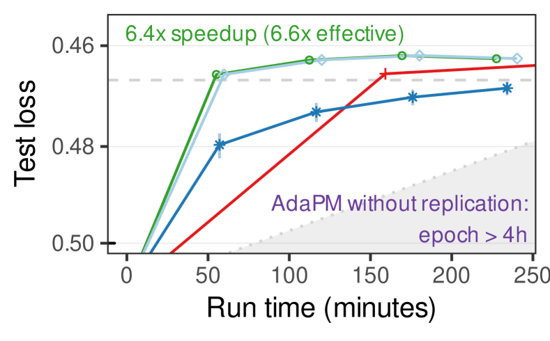
Some large-scale ML tasks are particularly hard to distribute because standard PM approaches are infeasible or inefficient. Currently, the most widely used approach is full static replication, i.e., to maintain a copy of the entire model at each cluster node. Static full replication is infeasible when the model size exceeds the memory capacity of a single node. It is also inefficient when the task accesses model parameters sparsely, i.e., when each update step reads and writes only a small subset of all parameters. This is because it synchronizes updates for all parameters to all nodes, even though each node accesses only a small subset at each point in time. Such sparse access is common in natural language processing (Mikolov et al., 2013; Pennington et al., 2014; Peters et al., 2018; Devlin et al., 2019), knowledge graph embeddings (Trouillon et al., 2016; Nickel et al., 2011; Balazevic et al., 2019; Bordes et al., 2013), some graph neural networks (Schlichtkrull et al., 2018; Shang et al., 2019; Vashishth et al., 2020), click-through-rate prediction (Cheng et al., 2016; Guo et al., 2017; Wang et al., 2017; Zhou et al., 2018), and recommender systems (Koren et al., 2009; Chen et al., 2012; Hu et al., 2008). Another standard PM approach—static parameter partitioning—partitions model parameters and transfers parameters to where they are needed on demand. This approach is often inefficient because of the access latency that this ad-hoc transfer induces (Renz-Wieland et al., 2020). Figure 1 shows that the performance of both these approaches (blue and red lines) falls behind that of a single node baseline for an example ML task, thus necessitating more advanced PM.

Figure 1. Performance for training large knowledge graph embeddings (ComplEx, dimension 500 on Wikidata5m) on an 8-node cluster. Static full replication and static parameter partitioning are easy to use, but inefficient. NuPS can be more efficient, but is hard to use. AdaPM is easy to use and efficient. Details in Section 5.1.

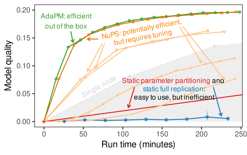
Advanced PM approaches can improve efficiency (Ho et al., 2013; Dai et al., 2015; Renz-Wieland et al., 2020; Zheng et al., 2021), but to do so, they require information about the underlying ML task. However, in current ML systems, this information is not readily available to the parameter manager. To work around this lack of information, existing advanced PM approaches require application developers to control critical PM decisions manually, by exposing configuration choices and tuning knobs. This requirement makes these PM approaches complex to use, such that their adoption in common ML systems remains limited. For example, multi-technique parameter managers (Zheng et al., 2021; Renz-Wieland et al., 2022) use different PM techniques (e.g., replication and dynamic allocation) for different parameters. This can be more efficient than simple PMs (e.g., see the performance of NuPS in Figure 1), but application developers need to specify upfront which technique to use for which parameter, and—for optimal performance—need to tune these technique choices. The absence of a general-purpose approach that is both simple to use and efficient gives rise to a range of custom, task-specific approaches that tightly couple PM to one specific ML task or one class of ML tasks (Lerer et al., 2019; Zhu et al., 2019; Zhao et al., 2020; Adnan et al., 2021; Miao et al., 2021; Peng et al., 2022). These approaches can be efficient, but they are not general-purpose leading to similar techniques being re-developed and re-implemented many times.

In this paper, we propose intent signaling, a general-purpose mechanism for providing the information that is necessary to enable tuning-free advanced PM for training with (some) sparse parameter access. Intent signaling cleanly decouples the application from PM: the application passes information about which parameters it intends to access before it does so, and the parameter manager acts based on these signals. We designed intent signaling in a way that can naturally be integrated into existing ML systems: the data loader can signal intent during batch preparation. We show that intent signaling not only simplifies the use of existing advanced PM approaches, it also enables a range of novel, more fine-grained, parameter managers that so far were impractical because PM had to be controlled manually.

In addition, we develop AdaPM, a proof-of-concept parameter manager that is based on intent signaling. AdaPM is (i) fully adaptive, i.e., it dynamically adapts all critical decisions to the underlying ML task, and (ii) zero-tuning, i.e., it adapts automatically, based purely on intent signals. To do so, AdaPM continuously re-evaluates what is the most efficient way to manage a specific parameter in the current situation (e.g., whether relocating the parameter is more efficient than replicating it). As the timing of PM actions (e.g., when to start maintaining a replica at a node) significantly affects performance, AdaPM continuously optimizes its action timing by learning from past timing decisions. AdaPM currently provides automatic PM among the main memory of cluster nodes.

We conducted an experimental evaluation on five ML tasks: training knowledge graph embeddings, word vectors, matrix factorization, click-through-rate prediction models, and graph neural networks. AdaPM was efficient across all tasks without requiring any tuning. In addition, it matched or even outperformed existing, manually tuned PM approaches. Figure 1 shows one example of this performance: AdaPM out of the box matched the performance of the best NuPS configuration, which was tuned specifically for this ML task.

In summary, our contributions are: (i) we analyze the complexity of existing PM approaches (Section 2), (ii) we propose intent signaling (Section 3), (iii) we describe AdaPM (Section 4), and (iv) we investigate the performance of AdaPM in an experimental study (Section 5).

Table 1. Approaches to distributed PM: adaptivity, ease of use, and efficiency for sparse workloads. Existing approaches adapt only individual system aspects to the underlying ML task and require applications to manually control these adaptations.

	Adaptivity
Approach	Replication	Parameter location	Choice of technique	Timing	Ease of use	Efficiency
Static full replication	static (full)	static	single	none	++	–
Static parameter partitioning (PS-Lite)	none	static	single	none	++	–
Selective replication (Petuum)	adaptive	static	single	by application	-	-
Dynamic allocation (Lapse)	none	adaptive	single	by application	–	-
Multi-technique PM (BiPS, Parallax)	static (partial)	static	static	none	–	+
Multi-technique PM (NuPS)	static (partial)	adaptive	static	by application	–	+
AdaPM (this paper)	adaptive	adaptive	adaptive	adaptive	+	++

2. Existing Approaches

Several general-purpose PM approaches aim to improve efficiency by adapting specific aspects to the underlying ML task. This adaptation requires information about the task. As this information is not available to the parameter manager in current ML systems, existing approaches rely on the application developers to manually control adaptation, which makes these approaches complex to use. In this section, we briefly discuss existing approaches, which aspects they adapt, and what makes them complex to use. Table 1 gives an overview. A more detailed analysis that also discusses efficiency can be found in Appendix A.

We discussed static full replication and static parameter partitioning in Section 1. These are implemented in many ML systems. For example, TensorFlow (Abadi et al., 2016) implements the two in the mirrored and parameter server distribution strategies, respectively; PyTorch (Paszke et al., 2019) implements them in the distributed data parallel and fully sharded data parallel wrappers, respectively. They are easy to use, but their efficiency is limited, as discussed in Section 1.

Selective replication (Xing et al., 2015) statically partitions parameters, and, to improve efficiency, selectively replicates parameters to further nodes during training. Existing approaches (Ho et al., 2013; Dai et al., 2015; Wei et al., 2015) are complex to use because they require applications to manually tune a staleness threshold parameter that affects both model quality and run time efficiency for each ML task.

Dynamic parameter allocation (Renz-Wieland et al., 2020) partitions parameters to nodes and, to improve efficiency, dynamically relocates parameters to the nodes that access them during training. Existing approaches are complex to use because they require the application to initiate parameter relocations manually in the application code and to tune the relocation offset (i.e., how long before an actual access the relocation is initiated).

Multi-technique parameter managers (Kim et al., 2019; Zheng et al., 2021; Renz-Wieland et al., 2022) support multiple PM techniques (e.g., replication, static partitioning, or dynamic allocation) and use a suitable one for each parameter. They are complex to use because they require the application to specify upfront which technique to use for which parameter. For optimal performance, application developers additionally need to tune these technique choices manually.

3. Intent Signaling

To enable automatic adaptive PM, we propose intent signaling, a novel mechanism that naturally integrates into ML systems. It passes information about upcoming parameter access from the application to the parameter manager. It decouples information from action, with a clean API in between: the application provides information (intent signals); the parameter manager transparently adapts to the workload based on the intent signals. In other words, all PM-related decision-making and knob tuning is done transparently by the parameter manager. The application only signals intent.

An intent is a declaration by one worker that this worker intends to access a specific set of parameters in a specific (logical) time window in the future. A natural choice of time window is a training batch. For example, a worker may signal that it will require access to, say, only 1M out of 100M parameters in batch 2 after analyzing the examples in that batch (e.g., embeddings of categories that do not appear in the batch are not needed). Such an approach integrates naturally with the data loader paradigm of common ML systems — such as Pytorch’s data loader (Paszke et al., 2019), TensorFlow’s data sets (Abadi et al., 2016), or the Gluon data loader (Chen et al., 2015) —, where training batches are constructed upfront in one or more separate threads and then queued until processed by the training thread(s) later on. This process is illustrated in Figure 2.

In general, it is important that intent is signaled before the parameter is actually accessed, such that the parameter manager can adapt proactively. We use logical clocks as a general-purpose construct for specifying the start and end points of intents. To ensure generality, each worker $i$ has one logical clock $C^{i}$ that is independent of other workers’ clocks. Each worker advances its clock with an advanceClock() primitive (as done in Petuum (Xing et al., 2015), but, in contrast to Petuum, invocation of our advanceClock() is cheap, as it only raises the clock). For example, a worker could advance its clock whenever it starts processing a new batch.

Figure 2. The data loader is a natural place to integrate intent signaling. After a batch $i$ is constructed, the data loader signals intent for the parameters $\mathcal{P}_{i}$ that are accessed in batch $i$.

We propose the following primitive for signaling intent:

$$\mathtt{Intent(\ parameters,\ \ \ C_{start},\ \ \ C_{end}\ \ \ [,type]\ )}$$

With this primitive, a worker signals that it intends to access a set of parameters in the time window between a start clock $\mathtt{C_{start}}$ (inclusive) and an end clock $\mathtt{C_{end}}$ (exclusive). The primitive allows to (optionally) specify intent type, e.g., read, write, read+write. Figure 2 illustrates an example of how the data loader can signal intent. With $\mathtt{Intent(\mathcal{P}_{2},2,3)}$, the data loader signals that the corresponding worker intends to access parameters $\mathtt{\mathcal{P}_{2}}$ (e.g., 1M out of 100M parameters) when at clock 2 (i.e., while it trains on batch 2). We say that an intent is inactive if it is signaled, but the worker has not reached the start clock yet, i.e., $\mathtt{C^{i}<C_{start}}$. We say that an intent is active if the worker clock is within the intent time window, i.e., $\mathtt{C_{start}\leq C^{i}<C_{end}}$. And we say that an intent is expired when the worker clock has reached the end clock, i.e., when $\mathtt{C_{end}\leq C^{i}}$. Invocation of the $\mathtt{Intent}$ primitive is meant to be cheap, i.e., it should not slow down the worker, even if the worker signals a large number of intents. Workers can flexibly combine intents: they can signal multiple (potentially overlapping) intents for the same parameter, extend one intent by signaling another later on, etc.

Intent signaling enables the PM to continuously adapt its parameter management strategy. This is in contrast to most existing PM approaches, where applications directly or indirectly control which or when actions such as selective replication are performed. As we will discuss in Section 4, intent signals allow AdaPM to choose suitable PM techniques dynamically during run time (as opposed to statically per parameter) and to time actions appropriately (as opposed to explicitly triggering actions). The key benefits of intent signaling are (i) ease of use, as applications do not need to make these hard choices (but only signal intent), and (ii) improved efficiency, as the PM can make better choices by carefully deciding which and when to perform actions.

4. The AdaPM Parameter Manager

Intent signaling opens a large design space for adaptive PM. Key design questions include: when and where to maintain replicas, whether and when to change parameter allocation, when to act on intent signals, how to synchronize replicas, how to exchange intent signals, on which nodes to make decisions, and how to communicate efficiently. We explore this space and describe AdaPM, a parameter manager that—in contrast to previous ones—is fully adaptive, i.e., it adapts all critical aspects to the underlying ML task, see Table 1. It does so automatically, based purely on intent signals, thus requiring no user input or knob tuning. And it does so dynamically, continuously re-evaluating what the most efficient approach is for the current situation. AdaPM has low overhead —a major design goal—and it takes all management decisions off the critical path of workers.

We give a brief overview of key design choices before we discuss the most challenging ones in detail. Figure 3 illustrates the architecture of AdaPM. We assume an architecture that—for efficiency—co-locates the parameter store in the same processes as the worker threads, as parameter managers commonly do (Ho et al., 2013; Huang et al., 2018; Renz-Wieland et al., 2020).

Figure 3. AdaPM architecture. For efficiency, AdaPM runs multiple worker threads in one process per node, and accesses locally available parameters via shared memory.

Adaptive choice of technique. AdaPM employs dynamic allocation and selective replication, and adaptively picks between the two per parameter. AdaPM dynamically chooses the most efficient technique for the current situation. Intuitively, AdaPM relocates a parameter if—at one point in time—only one node accesses the parameter. Otherwise, it creates replicas precisely where they are needed. We discuss AdaPM’s choice of technique in Section 4.1.

Adaptive action timing. AdaPM learns automatically when the right time to act on an intent signal is. This ensures that applications do not need to fine-tune the timing of their intent signals. They can simply signal their intents early, without sacrificing performance. See Section 4.2 for details.

Responsibility follows allocation. In AdaPM, the node that currently holds the main copy of a parameter (owner node) takes on the main responsibility for managing this parameter: it decides how to act on intent signals and acts as a hub for replica synchronization. For efficiency, this responsibility moves with the parameter whenever the it is relocated. This strategy generally reduces network communication as the responsibility for a parameter is always at a node that “needs” it. Details can be found in Section B.1 (page B.1 of the appendix).

(a) Decision

(b) Non-overlapping intents

(c) Partially overlapping intents

(d) Many concurrent intents (hotspot)

Figure 4. AdaPM decides automatically whether to relocate or replicate a parameter at any time $t$ (a). Example scenarios (b–d).

Efficient communication. AdaPM communicates for exchanging intent signals, relocating parameters, and managing replicas. To communicate efficiently, AdaPM locally aggregates intents, groups messages when possible to avoid small message overhead, and employs location caches to improve routing. Details can be found in Section B.2 (page B.2 of the appendix).

Optional intent. Intent signals are optional in AdaPM. An application can access any parameter at any time, without signaling intent. However, signaling intent makes access more efficient, as it allows AdaPM to avoid synchronous network communication.

4.1. Adaptive Choice of Technique

AdaPM receives intent signals from workers. Based on these intent signals, AdaPM tries to ensure that a parameter can be accessed locally at a node while this node has active intent for this parameter. To achieve this, AdaPM has to determine where to ideally allocate a parameter, if and where to create replicas, and for how long to maintain each replica.

To make parameters available locally, AdaPM employs (i) dynamic allocation and (ii) selective replication. That is, it (i) can relocate parameters among nodes and (ii) can selectively create replicas on subsets of nodes for specific time periods. AdaPM uses a simple heuristic rule to decide between the two: if, at one point in time, only one node has active intent for a parameter, AdaPM relocates the parameter to the node with active intent. After the node’s intent expires, AdaPM keeps the parameter where it is until some other node signals intent. In contrast, when multiple nodes have active intent for one parameter concurrently, AdaPM selectively creates a replica at each of the nodes when the intent of that node becomes active. It destructs the replica when the intent of that node expires. The simplicity of the decision rule allows AdaPM to communicate intent among nodes efficiently. Figure 4(a) illustrates AdaPM’s decision between relocation and selective replication. More involved approaches (or cost models) may provide further benefits, but this simple strategy performed remarkably well in our experimental study.

Let us consider three exemplary intent scenarios:

1. Two nodes have intent for the same parameter, and the active phases of the intents do not overlap; see Figure 4(b). AdaPM relocates the parameter from its initial allocation to the first node with intent and keeps it there even after the intent expires. AdaPM relocates the parameter to the second node with intent shortly before the node’s intent becomes active.

2. Two nodes have intent for the same parameter, and the active periods of the intents partially overlap; see Figure 4(c). AdaPM relocates the parameter to the first node with intent, then creates a replica on the second node while the two active intents overlap, and finally relocates the parameter to the second node after the intent of the first node expires.

3. Multiple nodes repeatedly have intent for the same parameter, see Figure 4(d). AdaPM creates replicas on all nodes with active intent. Whenever there is exactly one node with active intent (and the parameter is not currently allocated at this node), AdaPM relocates the parameter to this node.

AdaPM combines parameter relocation and replication because previous research has shown that their combination is beneficial (Renz-Wieland et al., 2022). Relocation is efficient for parameters that are accessed infrequently, as in the first example above, because the parameter value is transferred over the network only once per access (from where the parameter currently is to where the intent is). In contrast, replication can significantly reduce network overhead for frequently accessed parameters. In addition, unlike previous multi-technique approaches (Renz-Wieland et al., 2022; Zheng et al., 2021), AdaPM employs selective replication: AdaPM creates a replica precisely for the time during which it is needed. This increases efficiency as AdaPM does not need to maintain replicas while they are not needed. This also limits the impact of stale reads — which always arise when replication is used — since (i) AdaPM replicates as few parameters and as selectively as possible and continuously refreshes them (cf. Tab. 2) and (ii) no staleness occurs for reads of any non-replicated parameter. Further, unlike previous approaches, the choice of PM techniques for each parameter is dynamic: AdaPM can relocate the parameter at one point in time, and replicate it at another.

For making its decisions, AdaPM treats all intent types identically. More complex approaches could tailor their choices to intent type. For example, systems could choose to take different actions for read and write intents. In AdaPM, we keep the system simple and treat all intent types identically because we do not expect tailoring to improve performance for typical ML workloads: (i) applications typically both read and write a parameter and (ii) synchronous remote reads are so expensive that it is beneficial to provide a locally accessible value for a parameter even for a single read.

4.2. Adaptive Action Timing

AdaPM receives intent signals before the intents become active. I.e., there is an action window between the time the intent is signaled and the time the intent becomes active. AdaPM needs to determine at which point in this action window it should start to act on the intent signal, i.e., when it relocates the parameter or sets up a replica for this parameter. For example, consider the intent of node 3 in Figure 4(c): AdaPM needs to figure out at which point in time it starts maintaining a replica on node 3.

Relocating a parameter or setting up a replica takes some time. Consequently, if AdaPM acts too late and relocation or replica setup is not finished in time, remote parameter access is required. On the other hand, if AdaPM acts too early, it might maintain a replica longer than needed, inducing unnecessary communication. Furthermore, if AdaPM acts too early, it might use replication in scenarios in which—with better timing—relocation would have been both possible and more efficient. However, acting on an intent signal (slightly) too early is much cheaper than acting too late because the remote accesses caused by too late action slow down training significantly. In contrast, acting slightly too early merely causes over-communication. Thus, it is better to err on the side of acting too early.

The key challenge is that both (i) the preparation time for relocation or replica setup and (ii) the length of the action window are unknown. The action window length is unknown because it is unclear when the worker will reach the intent’s start clock. Both times are affected by many factors, e.g., by the application, the compute and network hardware, and the utilization of that hardware.

4.2.1. Learning When to Act

AdaPM aims to learn when the right time is to act on an intent signal. A general approach would estimate both preparation time and action window length separately. However, AdaPM acts on intent signals in point-to-point communication rounds that take a fairly constant amount of time. AdaPM thus simplifies the general approach and directly estimates the number of worker clocks per communication round. This allows AdaPM to decide whether an intent signal should be included in the current round or if it suffices to include the signal in a later round. A later round suffices if the next round will finish before the worker reaches the start clock of the intent.

As acting (slightly) too early is much cheaper than acting too late, our goal is to estimate a soft upper bound for the number of clocks during one communication round. I.e., we want to be confident that the true number of clocks only rarely (ideally, never) exceeds this soft upper bound. To this end, we employ a probabilistic approach in AdaPM: we assume that the number of clocks follows a Poisson distribution, estimate the (unknown) rate parameter for the distribution from past communication rounds, and use a high quantile of this Poisson distribution as a soft upper bound (e.g., the $0.9999$ quantile). In detail, we assume that the number of clocks by worker $i$ in round $t$ follows $\operatorname{Poisson}(\lambda^{i}_{t})$ with expected rate $\lambda^{i}_{t}$. We choose a Poisson distribution because it is the simplest, most natural assumption, and it worked well in our experiments. Note that we assume a Poisson distribution for a short time period (one round $t$ by one worker $i$), not one global distribution (a much stronger, unrealistic assumption, which, for example, would not account for changes in workload or system load).

Figure 5. AdaPM learns automatically when to act on an intent signal, using a probabilistic model to estimate a soft upper bound.

AdaPM acts on a given intent in round $t$ if it estimates that the corresponding worker might reach the start clock of the intent ($C_{\operatorname{start}}$) before round $t+1$ finishes, i.e., roughly if

$$C_{\operatorname{start}}<C^{i}_{t}+Q_{\operatorname{Poiss}}(2\cdot\lambda^{i}_{t},p)$$

where $C^{i}_{t}$ is the current clock of worker $i$ at the start of round $t$ and $Q_{\operatorname{Poiss}}(\lambda,p)$ computes the $p$ quantile of a Poisson distribution with rate parameter $\lambda$. Figure 5 illustrates this decision. Under our Poisson assumption, a $p=0.9999$ quantile gives a 99.99% probability that the actual number of clocks during the two rounds is below our estimate.

4.2.2. Estimating the Rate Parameter

Naturally, the true Poisson rate $\lambda^{i}_{t}$ is unknown. AdaPM estimates this rate from the number of clocks in past communication rounds, using exponential smoothing:

$$\hat{\lambda}^{i}_{t}\leftarrow(1-\alpha)\hat{\lambda}^{i}_{t-1}+\alpha(C^{i}_{t}-C^{i}_{t-1})$$

where $\hat{\lambda}^{i}_{t}$ is the estimate for the number of clocks by worker $i$ in round $t$ and $\alpha$ is the smoothing factor.

Input: Intent start $C_{\operatorname{start}}$, previous estimate $\hat{\lambda}^{i}_{t-1}$, clock of worker $i$ at the start of round $t$ ($C^{i}_{t}$) and round $t-1$ ($C^{i}_{t-1}$), smoothing factor $\alpha$, quantile $p$.

1:  $\Delta\leftarrow C^{i}_{t}-C^{i}_{t-1}$

2:  if $\Delta>0$ then

3:      $\hat{\lambda}^{i}_{t}\leftarrow(1-\alpha)\hat{\lambda}^{i}_{t-1}+\alpha(\Delta)$ ;

4:  else

5:      $\hat{\lambda}^{i}_{t}\leftarrow\hat{\lambda}^{i}_{t-1}$ ;

6:  end if

return $C_{\operatorname{start}}<C^{i}_{t}+Q_{\operatorname{Poiss}}(2\cdot\operatorname{max}(\hat{\lambda}^{i}_{t},\Delta),p)$;

Algorithm 1 Whether to act on a given intent in round $t$.

We consider two further aspects to improve the robustness of the estimate $\hat{\lambda}^{i}_{t}$. First, in ML training tasks, there commonly are periods in which the workers do not advance their clocks at all. For example, this is commonly the case at the end of an epoch, while training is paused for model evaluation. In such periods, the estimate would shrink. To keep it more constant, AdaPM does not update the estimate when the worker did not raise its clock during the previous communication round (i.e., if $C^{i}_{t}-C^{i}_{t-1}=0$).

Second, the observed number of clocks during round $t-1$ (i.e., $C^{i}_{t}-C^{i}_{t-1}=\Delta$) is not independent of the estimate $\hat{\lambda}^{i}_{t-1}$: if the estimate was too low, AdaPM did not act on some intents that the worker reached in this round, so that the worker was potentially slowed down drastically by remote parameter accesses. Thus, the estimate could settle in a “slow regime”. A large enough Poisson quantile (i.e., $p\gg 0.5$) ensures that the estimate grows out of such regimes over time. AdaPM further uses a simple heuristic to get out more quickly: if the number of clocks in the last round is larger than the current estimate, it uses this number rather than the estimate (i.e., it uses $\operatorname{max}(\hat{\lambda}^{i}_{t},\Delta)$).

Algorithm 1 depicts precisely how AdaPM decides whether to act on a given intent and how it updates the estimate.

4.2.3. Effect on Usability

AdaPM’s action timing relieves applications from the need to signal intent “at the right time”, as is, for example, required for initiating relocations in dynamic allocation PM approaches. It is important that applications signal intent early enough so that there is enough time for AdaPM to act on the signal. Below this lower limit, however, action timing makes AdaPM insensitive to when intent is signaled. Thus, applications can simply signal intent early, and rely on AdaPM to act at the right time.

AdaPM’s adaptive action timing introduces three hyperparameters: the smoothing factor $\alpha$, the quantile $p$, and the initial rate estimate $\hat{\lambda}^{i}_{0}$. However, these hyperparameters do not require task-specific tuning. We used the same configuration for all ML tasks and all experiments ($\alpha=0.1$, $p=0.9999$, and $\hat{\lambda}^{i}_{0}=10$). This configuration worked well across all five tested tasks, see Section 5.2.

5. Experiments

We conducted an experimental study to investigate whether and to what extent automatic fully adaptive PM is possible and beneficial. The source code, datasets, and information for reproducibility are available online.

In our study, we evaluated the performance of AdaPM by comparing it to efficient single-node baselines (Section 5.2), a manually tuned state-of-the-art parameter manager (Section 5.3), and standard PM approaches (Section 5.4). Further, we investigated whether and to what extent AdaPM benefits from supporting multiple management techniques (Sections 5.5 and 5.6), how scalable it is (Section 5.7), whether action timing is crucial for its performance (Section 5.8), how its performance compares to GPU implementations (Section 5.9). and which decisions it makes in practice (Appendix E ). Our major insights are: (i) AdaPM provided good speedups out of the box, without any tuning, (ii) AdaPM matched or even outperformed a manually tuned state-of-the-art parameter manager, (iii) AdaPM scaled efficiently, and (iv) adaptive action timing is a key building block for AdaPM’s efficiency. We conclude that automatic PM is possible and can be efficient.

5.1. Experimental Setup

Tasks. We considered five ML tasks: knowledge graph embeddings (KGE), word vectors (WV), matrix factorization (MF), click-through-rate prediction (CTR), and graph neural networks (GNN). The tasks differ in multiple ways, including the size of the models, the size of the data set, with what rate workers advance their clocks, and in their access patterns. In particular, some workloads exhibit a large amount of dense accesses (e.g., 52% for CTR), some very few (e.g., 0% for MF). We used common practices for task training, e.g., for partitioning training data and measuring model quality. When necessary, we tuned hyperparameters for each task on a single node and used the best found setting in all systems and variants. Appendix C describes each task in detail. Table 3 (in the appendix) provides an overview.

Baselines. We compared the performance of AdaPM to efficient single-node implementations, to NuPS (Renz-Wieland et al., 2022) (a state-of-the-art multi-technique parameter manager), to static parameter partitioning, to static full replication, and to three ablation variants. To ensure a fair comparison to NuPS, we ran six different hyperparameter configurations of NuPS for each task. Five configurations are designed to simulate a typical hyperparameter search by an application developer: a random search that is loosely informed by the NuPS heuristic and intuition, see Appendix D for details. In addition, we ran NuPS with the tuned hyperparameters from Renz-Wieland et al. (Renz-Wieland et al., 2022). These were tuned in a series of detailed experiments (but for a setting with 8 worker threads per node, not 32). Note that such detailed insights are not commonly available to application developers. As a single node baseline, we used an efficient shared memory implementation.

Implementation and cluster. We implemented AdaPM in C++, using ZeroMQ and Protocol Buffers for communication. We used a cluster of up to 16 Lenovo ThinkSystem SR630 computers, running Ubuntu Linux 20.04, connected with 100 Gbit/s Infiniband. Each node was equipped with two Intel Xeon Silver 4216 16-core CPUs, 512 GB of main memory, and one 2 TB D3-S4610 Intel SSD. We compiled code with g++ 9.3.0. The CTR and GNN tasks are implemented using PyTorch 1.12.1 and ran with Python 3.9.13. All other tasks are implemented in C++. We consistently used 32 worker threads per node and, unless specified otherwise, 8 cluster nodes. In NuPS and AdaPM, we additionally used 3 ZeroMQ I/O threads per node. In AdaPM, we used 4 communication channels per node; in NuPS, we used 1 channel as it supports only 1. As prior work, we use asynchronous SGD throughout so workers do not block. Thus, reads to non-replicated parameters (e.g., in static partitioning, NuPS, AdaPM) are always current. Reads to replicated parameters, however, may be stale (e.g., in full replication, NuPS, AdaPM). This staleness is generally bounded by the time between refreshs; see (Ho et al., 2013; Lian et al., 2015) for a convergence analysis under bounded staleness.

Measures. To keep costs controlled, we ran all variants with a fixed $4\text{\,}\mathrm{h}$ time budget. This time budget was sufficient for convergence for the fastest methods. We measured model quality over time and over epochs within this time budget. We conducted 3 independent runs of each experiment, each starting from a distinct randomly initialized model, and report the mean. For NuPS, we ran each of the 6 configurations once. We depict error bars for model quality and run time; they present the minimum and maximum measurements. In some experiments, error bars are not clearly visible because of small variance. Gray shading indicates performance that is dominated by the single node. We report two types of speedups: (i) raw speedup depicts the speedup in epoch run time, without considering model quality; (ii) effective speedup depicts the improvement w.r.t. time-to-quality. It is calculated from the time that each variant took to reach 90% of the best model quality that we observed in the single node. We chose this rather low threshold to determine speed-ups also for slower variants (which otherwise would not achieve the threshold in the time budget). The speed-ups for AdaPM at a higher accuracy, e.g., 99%, are near-identical to the ones at 90% (e.g., for CTR, 6.4x for both levels).

(a) Knowledge graph embeddings (KGE)

(b) Word vectors (WV)

(c) Matrix factorization (MF)

(d) Click-through-rate predication (CTR)

(e) Graph neural networks (GNN)

Figure 6. Performance of AdaPM on 8 nodes (32 threads per node), compared to efficient single-node baselines (Section 5.2), manually tuned PM (Section 5.3), standard PM approaches (Section 5.4), and single-technique AdaPM variants (Section 5.5).

5.2. Overall Performance (Figure 6)

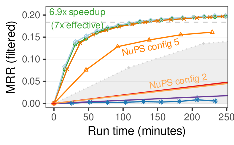
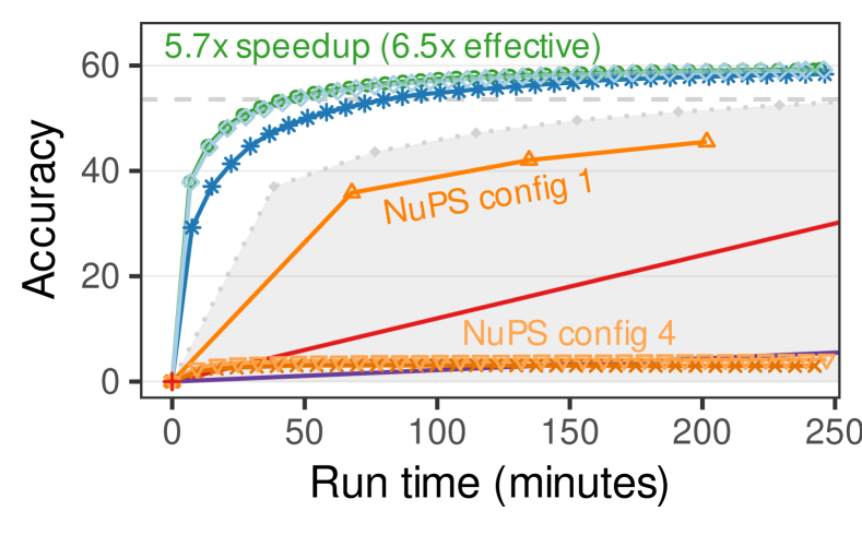
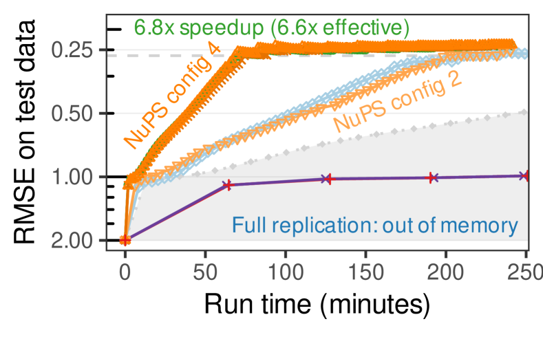
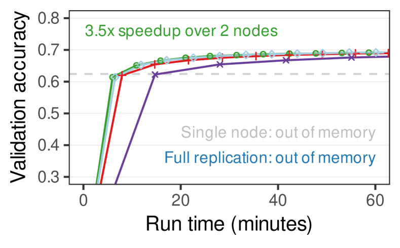
We ran AdaPM on all tasks, without any tuning, and compared its performance to the one of a single node. Figure 6 depicts the results. Figure 12 (page 12 of the appendix) additionally shows model quality per epoch. AdaPM achieved good speedups over the single node for all tasks out of the box, with 6.5x–7.0x effective speedups on 8 nodes.

We measured these speedups against the efficient shared-memory single-node implementation to ensure that they are practically relevant. Not comparing the performance of distributed implementations to single-node baselines or comparing to inefficient single-node implementations can be misleading (Renz-Wieland et al., 2020).

5.3. Comparison to Manually Tuned PM (Figure 6)

We further compared the performance of AdaPM to NuPS on the tasks for which NuPS implementations and tuned configurations are available (KGE, WV, and MF). Figures 6(a), 6(b), and 6(c) depict the results. AdaPM matched or even outperformed the performance of NuPS across all tasks.

NuPS required task-specific tuning to achieve good performance. The figures depict three of the six NuPS configurations: (i) the best and worst performing ones per task from our hyperparameter search and (ii) the ones tuned by the NuPS authors. Different configurations were efficient for different tasks. For example, configuration 4 was the best one for MF, but the worst one for WV.

AdaPM matched (MF) or outperformed (slightly in KGE and drastically in WV) the best NuPS configurations. AdaPM can outperform NuPS because AdaPM manages parameters more precisely, e.g., it maintained replicas only while needed, allowing it to synchronize fewer replicas more frequently. Appendix E provides more insight into how AdaPM works and how it differs from NuPS.

5.4. Comparison to Standard PM (Figure 6)

We compared AdaPM to static full replication and static parameter partitioning for all tasks. Again, Figure 6 shows the results. AdaPM outperformed standard PM.

Static full replication provided poor performance for all tasks but WV. It provided poor model quality for KGE and CTR because synchronizing full replicas on all nodes allowed for only infrequent replica synchronization. It ran out of memory for MF and GNN because their models are large. It worked well for WV because the WV model is small (only $14\text{\,}\mathrm{G}\mathrm{B}$, see Table 3) and the WV task is robust towards infrequent replica synchronization.

Static parameter partitioning was inefficient because it required synchronous network communication for the majority of parameter accesses. It was relatively efficient for GNN because this task accesses parameters in large groups, such that the impact of access latency is small.

Table 2. Per-epoch network communication and staleness.

Variant	Commun. (GB per node)					Mean replica staleness (ms)
	KGE	WV	MF	CTR	GNN	KGE	WV	MF	CTR	GNN
AdaPM	490	415	39	910	82	1.2	11.2	1.4	7.2	2.0
AdaPM w/o relocation	685	607	349	1066	171	1.4	13.8	7.7	7.7	2.6

5.5. Comparison to Single-Technique Adaptive PM (Figure 6)

We compared AdaPM to two ablation variants, see Figure 6. These variants are identical to AdaPM, but each variant is restricted to one management technique: AdaPM without relocation only replicates parameters, and AdaPM without replication only relocates parameters. AdaPM without replication was inefficient; AdaPM without relocation was efficient for most tasks.

AdaPM without replication performed poorly for all tasks because relocation is inefficient for hot spot parameters, as observed previously (Renz-Wieland et al., 2022).

AdaPM without relocation was efficient for KGE, WV, CTR, and GNN. For MF, it was 3.0x slower than AdaPM because the MF task exhibits locality (due to row-partitioning, each row parameter is accessed by only one node) and replication is inefficient for managing locality.

5.6. The Benefit of Relocation (Table 2)

As replication-only AdaPM performed well on many tasks (see Section 5.5), we further investigated whether it is beneficial for AdaPM to employ relocation in addition to replication. To do so, we measured the amount of communicated data and replica staleness. For simplicity, we take the time since the last replica refresh (i.e., the last check for updates) as staleness and ignore whether or not the value has actually changed since then. Table 2 depicts the results. Besides improving performance for some tasks (see Section 5.5), employing relocation reduced network overhead and decreased replica staleness for all tasks.

The contrast in communication and staleness was particularly large for tasks with locality (MF and GNN due to data partitioning), where AdaPM communicated up to 9x fewer data. But supporting relocation also improved efficiency for all other tasks. For example, AdaPM without relocation communicated 40% more data for one KGE epoch because relocation is more efficient if two nodes access a parameter after each other: relocation sends the parameter directly from the first to the second node, whereas replication synchronizes via the owner node.

5.7. Scalability (Figure 7)

(a) KGE: raw

(b) WV: raw

(c) MF: raw

(d) KGE: effective

(e) WV: effective

(f) MF: effective

Figure 7. Scalability (logarithmic axes). Raw speedup (a-c), i.e., w.r.t. epoch run time, and effective speedup (d-f), i.e., w.r.t. reaching 90% of the best model quality observed on a single node. Runs that did not reach this threshold within the time limit are not shown.

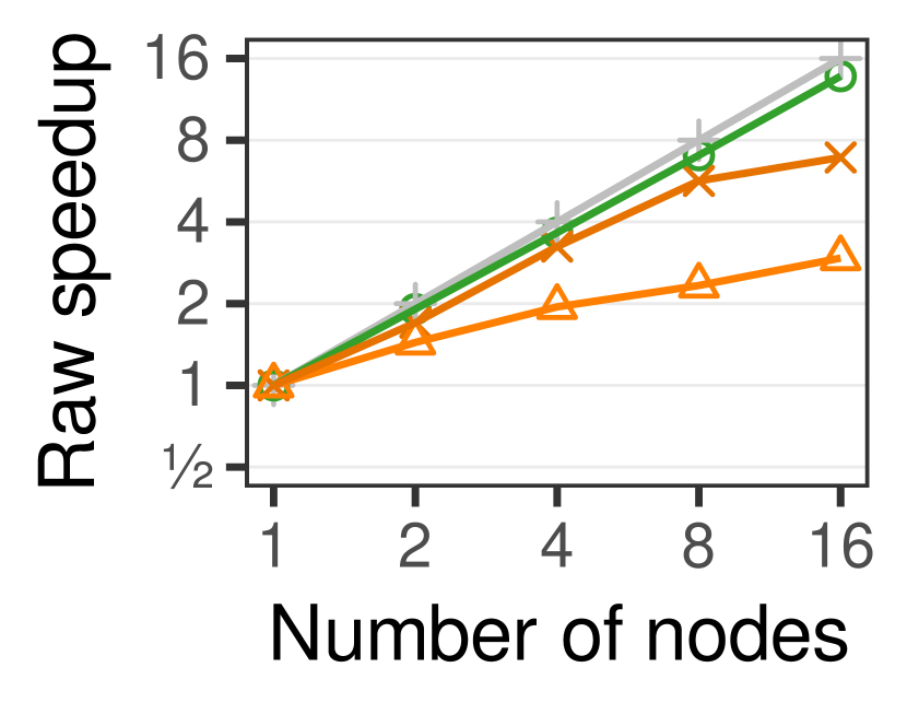
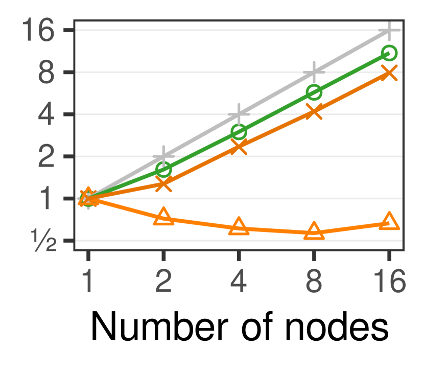
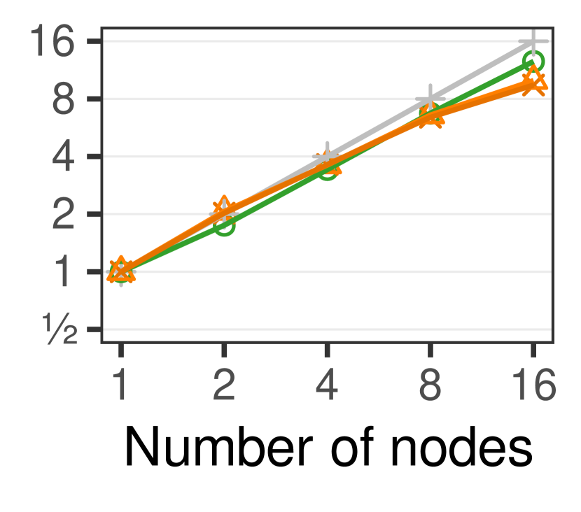
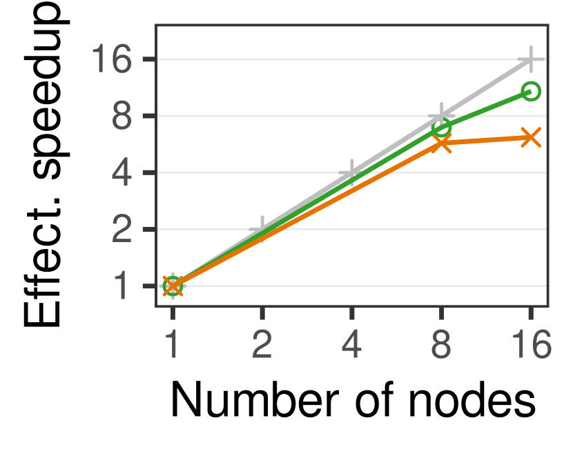
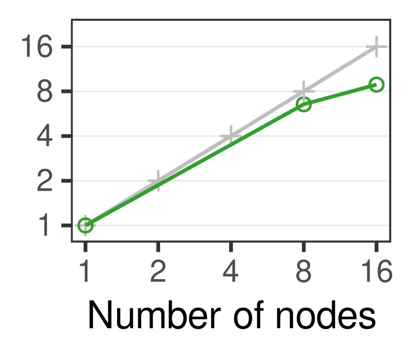
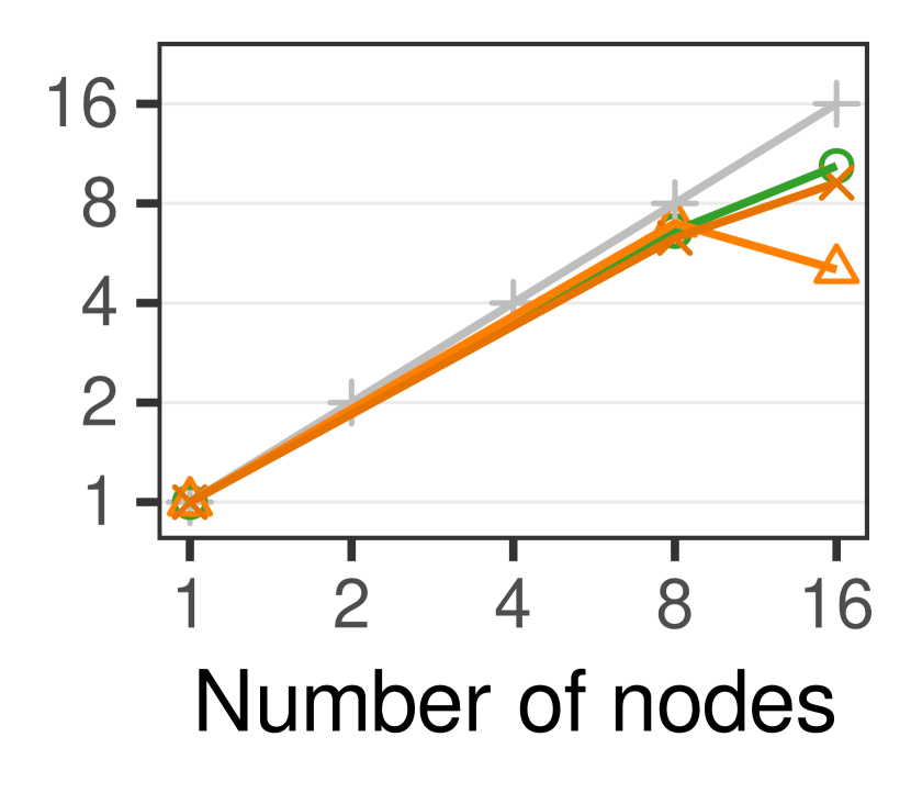
We investigated the scalability of AdaPM and compared it to NuPS. Figure 7 depicts raw and effective speedups over the single node for KGE, WV, and MF; Figure 13 (page 13) does so for the other tasks. AdaPM scaled efficiently, achieving near-linear raw and good effective speedups.

AdaPM scaled more efficiently than NuPS because NuPS’s scalability was limited by relocation conflicts (i.e., concurrent accesses to a relocation-managed parameter). For example, in KGE, the share of remote accesses in the best found NuPS configuration was 1.2%, 2.4%, 3.4%, and 5.3% on 2, 4, 8, and 16 nodes, respectively; in AdaPM, it was <0.0001%. The effective speedups slightly dropped on 16 nodes because we tuned task hyperparameters (e.g., learning rate and regularization) for the single node and—to minimize the impact of hyperparameter tuning—used these settings throughout all experiments. These settings were not optimal for runs with 16x more parallelism. Other settings achieved better effective scalability.

5.8. Effect of Action Timing (Figure 8)

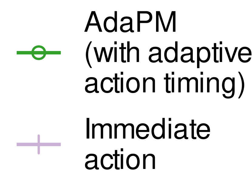
To investigate the effect of action timing, we compared AdaPM to an ablation variant that acts immediately after each intent signal, on workloads with varying signal offsets. Figure 8 depicts the results for WV, see Figure 14 (page 14) for further tasks. With adaptive action timing, AdaPM was efficient for any sufficiently large signal offset.

(a) Epoch run time

(b) Model quality

Figure 8. The effect of adaptive action timing for WV on epoch run time (a) and on model quality after one epoch (b).

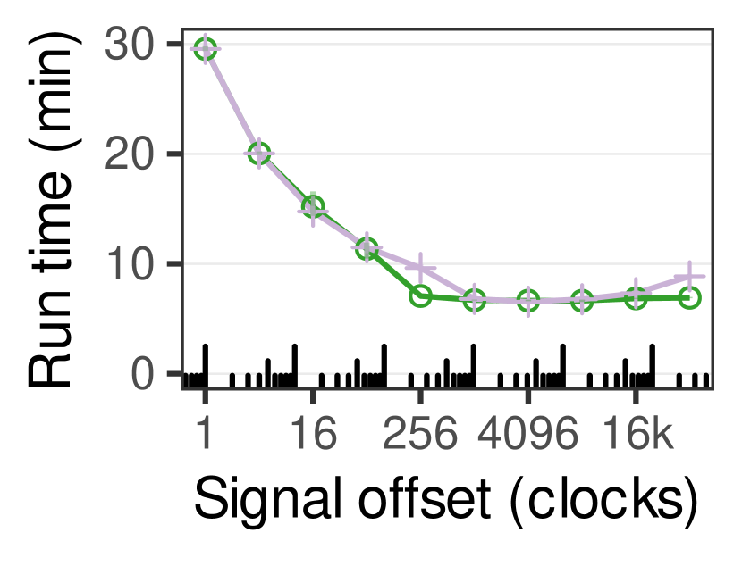
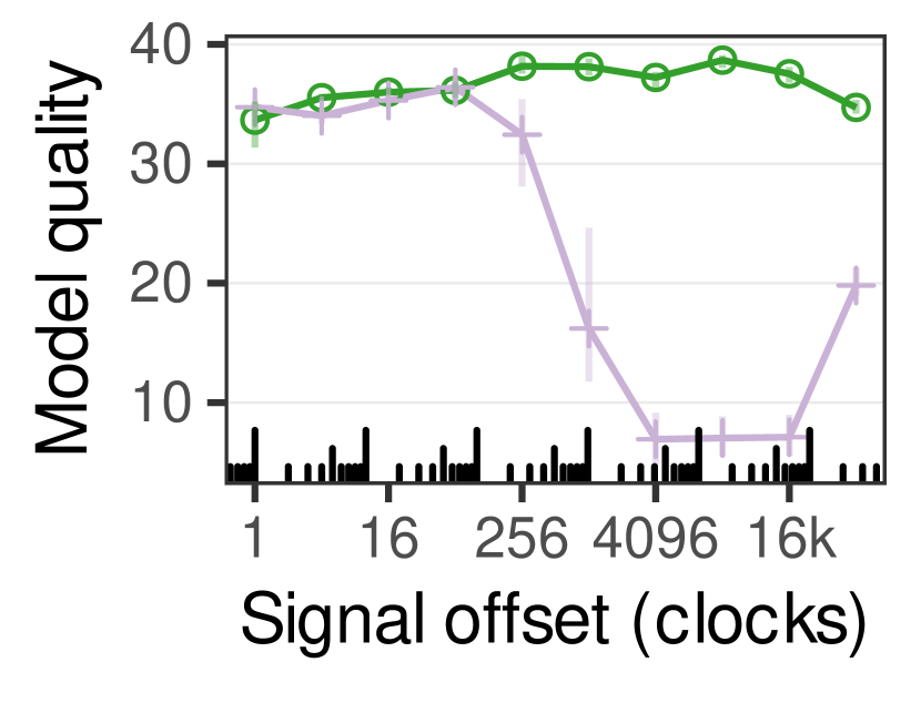
Early signals. With adaptive action timing, AdaPM provided excellent performance for all large signal offset values. In contrast, with immediate action, performance was poor for large signal offsets: run time increased and model quality decreased. The reason for this was that the immediate action variant maintained replicas for longer than necessary (thus lowering synchronization frequency).

Late signals. Smaller relocation offsets improved performance for immediate action, but did not further improve performance for AdaPM. For both, epoch run time was poor when intent was signaled so late that the system did not have sufficient time for setting up replicas or relocating parameters. Thus, there was a task-specific optimum value for immediate action (necessitating tuning), but not for AdaPM.

5.9. Comparison to GPU Implementations

CTR and GNN models are typically trained on GPUs, whereas we used CPUs in our proof-of-concept implementation of AdaPM. To put our results in perspective, we briefly compared to recent GPU-based methods for these two tasks. Some overhead is expected because these methods are task-specific, i.e., they use specialized and tuned training algorithms that cannot be used for other tasks directly, whereas AdaPM is general-purpose. Although the CPU and GPU settings are very different and cannot be compared directly, we found that the results obtained by AdaPM seem competitive.

For CTR, Zheng et al. (Zheng et al., 2022) ran one epoch on a 90% train split of our dataset, for the same model, and with comparable batch size in 76.8 minutes on one V100 GPU. AdaPM took 57.5 minutes on 8 CPU nodes for a 85.7% train split. The key bottleneck of GPU-based methods is data transfer to and from GPU memory as the models do not fit in GPU memory. Very large batch sizes can mitigate this to some extent, but require careful work to avoid loss of accuracy (Zheng et al., 2022).

For GNN, Min et al. (Min et al., 2021) ran one epoch on the same dataset, but with a different model, on 2 RTX 3090 GPUs in 10.2 minutes. AdaPM ran 1 epoch in 5.3 minutes on 8 CPU nodes. MariusGNN (Waleffe et al., 2022) achieved a validation accuracy of 0.6638 in 8.2 minutes on the same dataset (with a slightly different model) using 1 V100 GPU. Waleffe et al. (Waleffe et al., 2022) further report that DGL (Wang et al., 2019b) required 4 V100 GPUs to achieve the same accuracy in similar time. AdaPM achieved slightly better accuracy (0.665) after 15.5 minutes using 8 CPU nodes.

6. Conclusion

We proposed intent signaling, a novel mechanism that decouples providing information about parameter accesses (simple) from how and when it is exploited (hard). Intent signaling increases ease of use and efficiency in parameter management. We presented AdaPM, a parameter manager that automatically adapts to the underlying ML task based solely on intent signals. In our experimental study, AdaPM was efficient for many ML tasks out of the box, without requiring any tuning, and matched or even outperformed state-of-the-art (more complex to use) systems. Interesting directions for future work are how to better integrate co-processor (e.g, GPU) memory in an adaptive parameter manager such as AdaPM and how to support intent signaling directly in common ML systems.

(a) Static full replication

(b) Static parameter partitioning

(c) SSP selective replication

(d) ESSP selective replication

(e) Dynamic allocation

(f) Multi-Technique PM

(g) AdaPM (this paper)

Figure 9. Parameters held by different nodes at different times (initially; and early and late during training) in common parameter management approaches. One square depicts one parameter. A node either cannot access the parameter locally ( ), holds the main copy of the parameter ( ), or holds a replica of the parameter ( ).

Appendix A Efficiency and Complexity of Existing Approaches

In the following, we analyze existing general-purpose PM approaches w.r.t. their ease of use, their efficiency for sparse ML tasks (i.e., tasks in which each update step accesses only a small subset of all model parameters), and in which aspects they are adaptive. Figure 9 illustrates existing approaches. Table 1 (page 1) summarizes our analyses.

A.1. Static Full Replication

Static full replication replicates the full model to all cluster nodes statically (i.e., throughout training) and synchronizes the replicas periodically, either synchronously (triggered by the application) or asynchronously in the background. This approach is currently popular for training dense neural networks (LeCun et al., 1989; Sergeev and Balso, 2018; Li et al., 2020), in particular with synchronous synchronization after stochastic gradient descent (SGD) mini-batches. As it is entirely static, it requires no run time information from the application. So it is relatively easy to use. (It does, however, require the application to either trigger replica synchronization or to set the frequency of background synchronization.) Parameter access is fast, as every worker can access every parameter locally, without synchronous network communication. However, full replication is communication-inefficient for sparse workloads (Renz-Wieland et al., 2022), as it maintains the replicas of all parameters on all nodes throughout the training task, even though each node accesses only a small subset of these replicas at each point in time. Also, full replication limits model size to the memory capacity of a single node. In summary, full replication is very easy to use, but inefficient for sparse workloads because it over-communicates.

A.2. Static Parameter Partitioning

Static parameter partitioning (as done in classic parameter servers (Smola and Narayanamurthy, 2010; Ahmed et al., 2012; Li et al., 2014)) partitions the model parameters to the cluster nodes and provides global reads and writes to the parameters by transparently sending messages to the corresponding nodes. No replicas are created. Static parameter partitioning is easy to use: it requires no information from the application and no hyperparameter tuning. However, the approach is inefficient because the vast majority of parameter accesses involve synchronous network communication for sending messages to the node that holds the parameter (Renz-Wieland et al., 2020). In summary, static parameter partitioning is very easy to use, but inefficient due to synchronous network communication.

A.3. Selective Replication

A selective replication parameter manager, such as Petuum (Xing et al., 2015), statically partitions parameters. During training, it adaptively replicates a subset of the parameters to nodes that access these parameters. Potentially, this makes PM more efficient, as replicas can be used to process repeated accesses to the same parameter locally. Petuum sets up a replica for a specific parameter at a specific node reactively when a worker on that node accesses the parameter. Thus, the workers have to wait for replicas to be set up synchronously.

Petuum supports two heuristics to decide how long to maintain a replica at a node after parameter access: SSP (Ho et al., 2013) and ESSP (Dai et al., 2015). SSP maintains a replica for an application-specified number of logical clocks, the so-called staleness bound. Applications have to tune this staleness bound specifically for each task, as the staleness bound impacts both model quality and run time efficiency. This tuning makes SSP complex to use. Further, SSP is inefficient for many tasks because, for realistic staleness bounds, no replicas are set up for the majority of parameter accesses, so that workers have to wait for synchronous replica setup frequently. In summary, an SSP parameter manager is complex to use because it requires tuning and inefficient because of synchronous replica setup.

ESSP is a coarse heuristic that also creates a replica when a parameter is accessed at a node, and then maintains the replica throughout the entire training task. This mitigates the inefficiency of reactive replica creation (as each replica is set up only once), at the cost of over-communication. For many workloads, after a short setup phase, ESSP is essentially equivalent to full replication, i.e., it holds a full model replica on every node, although only a small part of the model is accessed at every point in time. This makes ESSP inefficient for sparse workloads (Renz-Wieland et al., 2022). In summary, an ESSP parameter manager is complex to use, and inefficient due to over-communication.

A.4. Dynamic Parameter Allocation

A dynamic parameter allocation parameter manager, such as Lapse (Renz-Wieland et al., 2020), adaptively changes the location of parameters during training, i.e., it relocates parameters among nodes. The advantage of relocating is that parameters can then be accessed locally, without network communication, at the respective nodes, and no replica synchronization is required. Key for the efficiency of a dynamic allocation PM is that parameter relocation is proactive, i.e., that parameter relocation runs asynchronously and is finished before the parameter is accessed. PM lacks the necessary information to initiate relocations proactively. Thus, Lapse requires the application to initiate parameter relocations manually via an additional localize primitive. Application developers are required to add appropriate invocations to their application code and—for optimal performance—tune the relocation offset, i.e., how long before the actual access parameter relocation is initiated. Relocation should be early enough such that it is finished when the parameter is accessed, but not too early to minimize the probability of relocating the parameter away from other nodes that are still accessing it. Offloading these performance-critical decisions to the application makes dynamic allocation PM complex to use and leads to potentially sub-optimal performance. In addition, dynamic allocation PM is inefficient for many real-world ML tasks because they are inefficient for hot spots, i.e., parameters that are frequently accessed by multiple nodes concurrently (Renz-Wieland et al., 2022). In summary, dynamic parameter allocation is complex to use, and inefficient for many ML tasks.

A.5. Multi-Technique Parameter Management

Multi-technique parameter managers support multiple parameter management techniques (e.g., replication, static partitioning, or relocation) and let the application pick a suitable one for each parameter. Parallax (Kim et al., 2019) and BiPS (Zheng et al., 2021) support static full replication (i.e., creating replicas on all nodes) and static partitioning. NuPS (Renz-Wieland et al., 2022) supports static full replication and dynamic parameter allocation. The choice of technique is static: for each parameter, the application picks one technique before training, which is then used throughout. Using a suitable technique for each parameter can improve PM efficiency (Renz-Wieland et al., 2022; Zheng et al., 2021; Kim et al., 2019). However, it requires information about the workload. As these parameter managers decide on a technique for each parameter before training, they require this information upfront. There are heuristics that pick a technique for each parameter (Kim et al., 2019; Renz-Wieland et al., 2022). These heuristics require access frequency statistics and do not consistently achieve optimal performance. Thus, manual tuning can be required to achieve high efficiency. These information and tuning requirements make multi-technique PM very complex to use and—if not tuned appropriately—lead to sub-optimal performance. NuPS additionally requires the application to manually trigger relocations (as in Lapse), further complicating its use. In summary, multi-technique PM can be efficient, but is very complex to use.

Appendix B AdaPM Architecture Details

B.1. Responsibility Follows Allocation

Based on intent signals, AdaPM decides when to relocate a parameter and when to maintain a replica on which node. Two important design decisions to enable this precise management are: (i) which node makes these decisions and (ii) when replicas exist, how to keep them synchronized (efficiently)? A key feature of AdaPM is that the node at which a parameter is currently allocated—the owner node of the parameter—takes the main responsibility for both. The owner node decides whether to relocate a parameter and where to maintain replicas (Section B.1.1); and the owner node acts as a hub for replica synchronization (Section B.1.2). Placing responsibility at the owner node reduces network overhead and can reduce processing load because the owner node changes whenever the parameter is relocated, such that responsibility is close to where the parameter and the associated processing is.

B.1.1. Choice of Management Technique

(a) Static responsibility

(b) Dynamic responsibility

Figure 10. Network communication for placing management responsibility (a) on the statically assigned home node (node 0) or (b) on the dynamically changing owner node.

AdaPM chooses a technique based on the intent signals of all nodes for a parameter. Thus, the intent signals of all nodes for one parameter need to come together at one node, such that this node can make this decision.

This decision could be made by a node that is statically assigned to a parameter (e.g., by hash partitioning). We call such a statically assigned node the home node (van Steen and Tanenbaum, 2017). In the static approach, nodes continuously send their intent signals for parameter $k$ to the parameter’s home node. The home node decides whether to relocate or replicate the parameter, and instructs the current owner of parameter $k$ to act accordingly. The advantage of this static approach is that it is straightforward to route intent signals, as the signals for one key are sent to the same node throughout training. Its disadvantage is that the home node is always involved, even when it does not have intent itself (a common disadvantage of home-based approaches in distributed systems (van Steen and Tanenbaum, 2017)). Figure 10(a) illustrates the communication for the static approach. Even while there is intent only at node 2 and the parameter is allocated at node 2, node 2 needs to communicate its intent to the home node (node 0), such that the home node can decide to keep the parameter allocated at node 2. While there is intent at nodes 2 and 3, both nodes need to communicate their intent to node 0.

To overcome this problem, AdaPM makes these decisions on the owner node of the parameter, i.e., the node where the parameter is currently allocated. This node changes whenever the parameter is relocated. The key advantage of this approach is that the home node does not need to be involved, reducing network traffic and processing load. Figure 10(b) illustrates the communication for this dynamic approach. After an initial communication of intent (and a subsequent relocation), no further communication between node 2 and node 0 is necessary, as node 2 makes any decisions about the parameter locally. While there is intent on node 2 and node 3, node 3 communicates its intent directly to node 2, without involving node 0. A disadvantage of the dynamic approach is that routing becomes more complex, as the owner node changes throughout training. To overcome this disadvantage, AdaPM employs location caches, which enables nodes to send their intent signals to the current owner node directly, most of the time, see Section B.2.3.

B.1.2. Replica Synchronization

While a parameter is replicated, multiple nodes hold a copy of the value of the parameter and write updates to this local copy. For convergence, it is crucial that these copies are synchronized, i.e., that updates of one node are propagated to the replicas on other nodes. AdaPM employs relocation and selective replication (as discussed in Section 4.1). Consequently, for the majority of parameters, at a given time, only few nodes (if at all) hold a replica for a given parameter. Thus, replica updates have to be propagated only to a small subset of all nodes. Further, this subset is different for each parameter and changes constantly and potentially rapidly. These two properties make AllReduce or gossip-based synchronization approaches unattractive for AdaPM. Instead, AdaPM propagates replica updates via the owner node of a parameter: replica holders send updates to the parameter’s owner, which then propagates them to other replica holders.

To use the network efficiently, AdaPM batches replica updates (as, e.g., Petuum (Xing et al., 2015) does). As Petuum, AdaPM does so for both directions of update propagation: from replica holders to the owner node and from the owner node to the replica holders. To further improve efficiency, AdaPM versions parameter values and communicates deltas: when nodes request updates for their replicas, they include the version number that is locally available; the owner node sends only those updates that the requesting node has not received previously.

B.2. Efficient Communication

AdaPM communicates to exchange intent signals, to relocate parameters, to set up and destruct replicas, and to synchronize replicas. Key for the overall efficiency of AdaPM is that this communication is efficient. In this section, we discuss several design aspects of AdaPM that improve communication efficiency: AdaPM locally aggregates intent signals and sends aggregated intent signals over the network (Section B.2.1), groups messages (Section B.2.2), employs location caches for more efficient routing (Section B.2.3), and relocates parameters only when there is exactly one node with active intent (Section B.2.4).

B.2.1. Aggregated Intent

As discussed in Section B.1.1, for each parameter, there is one (dynamically changing) node that decides whether to relocate or replicate a specific parameter. To enable this decision, all other nodes need to continuously send their intent signals for this specific parameter to this decision-making node.

A naive approach to intent communication is that all workers eagerly send each intent (i.e., a tuple of parameter, start clock, end clock, intent type, and worker id) to the node that makes decisions immediately after the intent is signaled. Additionally, workers regularly send the state of their clocks (potentially by piggybacking on other messages). The decision-making node stores all intents, determines which of them are active, and decides based on this perfect view of all intents for this specific parameter. However, this naive approach induces significant network overhead, as a large number of intent signals have to be sent over the network constantly. Especially for hot spot parameters, for which there are many intent signals, this can be prohibitive.

AdaPM employs a more communication-efficient approach: each node stores inactive intents locally, determines which ones should be treated as active, and sends aggregated information about active intents to the decision-making node. More precisely, each node communicates to the decision-making node when intent becomes active and it communicates when intent expires. The node does not communicate which or how many workers have active intent. This requires significantly less network communication, especially for hot spot parameters. The disadvantage is that the decision-making node has less information. Precisely, it does not know about inactive intents or how long active intent will last. For the decisions that AdaPM makes, this information is not required, such that AdaPM adopts the more communication-efficient approach.

B.2.2. Message Grouping

Adaptive action timing ensures that a parameter is relocated or a replica is set up asynchronously, i.e., before a worker accesses the parameter. This allows AdaPM to improve network efficiency by grouping messages for communicating (aggregated) intent signals, for relocating parameters, and for creating, destructing, and synchronizing replicas into one request–response message protocol.

In more detail, to send a synchronization request, a dedicated thread at a node collects (i) a list of parameters for which local workers have active intent and (ii) all updates to local replicas. The node sends these to the owners of the corresponding parameters in a synchronization request. Each owner (i) merges the replica updates into its parameter store and (ii) responds to each intent signal (with parameter relocation or replica setup). It does so in one (grouped) synchronization response. By default, AdaPM triggers a synchronization request as soon as the last communication round has finished. To reduce the network and CPU load for synchronization, AdaPM allows for limiting the number of communication rounds per second.

B.2.3. Routing

In AdaPM, nodes send intent signals and replica updates to the current owner node. This owner node can change dynamically during run time. To route messages, AdaPM adapts the home node forwarding approach (with location caches) of Lapse (Renz-Wieland et al., 2020). We briefly describe this approach below and refer to Renz-Wieland et al. (Renz-Wieland et al., 2020) for a more detailed discussion.

As fallback, there is one home node for each parameter. This home node is assigned statically to each parameter (by hash partitioning). The home node knows which (other) node is currently the owner of the parameter. If any node does not know where a parameter is currently allocated, it sends its message to the home node, which then forwards the message to the current owner. Whenever a parameter is relocated, the old owner node informs the home node of this relocation. These location updates are piggybacked onto synchronization messages.

To increase efficiency, AdaPM additionally employs location caches. I.e., each node locally stores the last known location for parameters that it accessed in the past. This allows for sending updates and intent signals directly to the current owner. AdaPM uses synchronization responses, outgoing parameter relocations, and responses to remote parameter accesses to update location caches. It does not explicitly invalidate location caches. Instead, it tolerates that messages can be routed based on stale ownership information and relies on the receiving nodes to forward the messages to the current owner (via the home node, see Renz-Wieland et al. (Renz-Wieland et al., 2020) for a more detailed discussion). Location caches are more important in AdaPM than in Lapse as there are scenarios in AdaPM in which nodes repeatedly send messages to the owner node. In particular for hot spot parameters, the owner node changes rarely (see, e.g., Figure 4(d)), such that nodes send their signals and updates to the same owner node repeatedly.

B.2.4. Parameter Relocation

(a) Relocate only when exactly     one node has active intent

(b) Relocate immediately when the owner’s intent expires

Figure 11. AdaPM relocates a parameter only when there is exactly one node with active intent (and the parameter is currently not allocated at this node).

AdaPM relocates parameters only when there is (at one point in time) exactly one node with active intent, and this node does currently not hold the parameter. It does not relocate a parameter while multiple nodes have active intent, even if the intent of the current owner expires. Figure Figure 11 illustrates this approach. AdaPM employs this approach because relocating in the presence of replicas would require (i) to update routing information on each replica holder (see Section B.2.3) and (ii) to transfer intent information to another node (see Section B.1.1).

Table 3. ML tasks, models, and datasets.

Task	Model parameters				Data
	Model	Keys	Values	Size	Dataset	Data points	Size
Knowledge graph embeddings	ComplEx, dim. $500$	$4.8\text{\,}\mathrm{M}$	$4.8\text{\,}\mathrm{B}$	$35.9\text{\,}\mathrm{G}\mathrm{B}$	Wikidata5M	$21\text{\,}\mathrm{M}$	$317\text{\,}\mathrm{M}\mathrm{B}$
Word vectors	Word2Vec, dim. $1000$	$1.9\text{\,}\mathrm{M}$	$1.9\text{\,}\mathrm{B}$	$14.0\text{\,}\mathrm{G}\mathrm{B}$	1b word benchmark	$375\text{\,}\mathrm{M}$	$3\text{\,}\mathrm{G}\mathrm{B}$
Matrix factorization	Latent Factors, rank 1000	$11.0\text{\,}\mathrm{M}$	$11.0\text{\,}\mathrm{B}$	$163.9\text{\,}\mathrm{G}\mathrm{B}$	$10\text{m}\times 1\text{m}$ matrix, zipf 1.1	$1000\text{\,}\mathrm{M}$	$31\text{\,}\mathrm{G}\mathrm{B}$
Click-through-rate prediction	Wide & Deep, dim. $128$	$67\text{\,}\mathrm{M}$	$8.7\text{\,}\mathrm{B}$	$32.5\text{\,}\mathrm{G}\mathrm{B}$	Criteo Kaggle	$46\text{\,}\mathrm{M}$	$7\text{\,}\mathrm{G}\mathrm{B}$
Graph neural networks	GCN, dim. $500$	$111\text{\,}\mathrm{M}$	$111.1\text{\,}\mathrm{B}$	$413.7\text{\,}\mathrm{G}\mathrm{B}$	ogbn-papers100M	$111\text{\,}\mathrm{M}$	$56\text{\,}\mathrm{G}\mathrm{B}$

Appendix C Task details

Knowledge graph embeddings. KGE models learn algebraic representations of the entities and relations in a knowledge graph. For example, these representations have been applied successfully to infer missing links in knowledge graphs (Nickel et al., 2016). This task, based on Liu et al. (Liu et al., 2017), trains ComplEx (Trouillon et al., 2016) (one of the most popular KGE models) embeddings using SGD with AdaGrad (Duchi et al., 2011) and negative sampling (Ruffinelli et al., 2020; Liu et al., 2017). To generate negative samples, both the subject and the object entity of a positive triple are perturbed $n_{\operatorname{neg}}$ times, by drawing random entities from a uniform distribution over all entities (we used a common setting of $n_{\operatorname{neg}}=100$ (Ruffinelli et al., 2020)). We used the Wikidata5M dataset (Wang et al., 2019a), a real-world knowledge graph with $4\,818\,679$ entities and $828$ relations, and a common embedding size of $500$ (Ruffinelli et al., 2020). We partitioned the subject–relation–object triples of the dataset to the nodes randomly, as done in (Kochsiek and Gemulla, 2021). We used LibKGE (Broscheit et al., 2020) (commit 3146885) to evaluate models and report the mean reciprocal rank (filtered) (MRRF) as model quality.

Word vectors. WVs are a language modeling technique in natural language processing: each word of a vocabulary is mapped to a vector of real numbers (Mikolov et al., 2013; Pennington et al., 2014; Peters et al., 2018). These vectors are useful as input for many natural language processing tasks, for example, syntactic parsing (Socher et al., 2013) or question answering (Liu et al., 2018). This task, based on Mikolov et al. (Mikolov et al., 2013), uses SGD with AdaGrad (Duchi et al., 2011) and negative sampling to train the skip-gram Word2Vec (Mikolov et al., 2013) model (dimension 1000) on the One Billion Word Benchmark (Chelba et al., 2013) dataset (with stop words of the Gensim (Řehůřek and Sojka, 2010) stop word list removed). We used common model parameters (Mikolov et al., 2013) for window size (5), minimum count (1), and frequent word subsampling (0.01). We measured model accuracy using a common analogical reasoning task of $19\,544$ semantic and syntactic questions (Mikolov et al., 2013).

Matrix factorization. Low-rank MF is a common tool for analyzing and modeling dyadic data, e.g., in collaborative filtering for recommender systems (Koren et al., 2009). This task, based on Teflioudi et al. (Teflioudi et al., 2012), uses SGD with AdaGrad (Duchi et al., 2011) to factorize a synthetic, Zipf-1.1 distributed $10\text{m}\times 1\text{m}$ dataset with 1b revealed cells, modeled after the Netflix Prize dataset. Data points were partitioned to nodes by row and to workers within a node by column. Each worker visited its data points by column (to create locality in column parameter accesses), with random order of columns and of data points within a column. We report the root mean squared error (RMSE) on the test set as metric for model quality.

(a) Knowledge graph embeddings (KGE)

(b) Word vectors (WV)

(c) Matrix factorizaton (MF)

(d) Click-through-rate prediction (CTR)

(e) Graph neural networks (GNN)

Figure 12. Model quality per epoch.

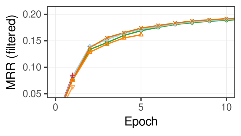
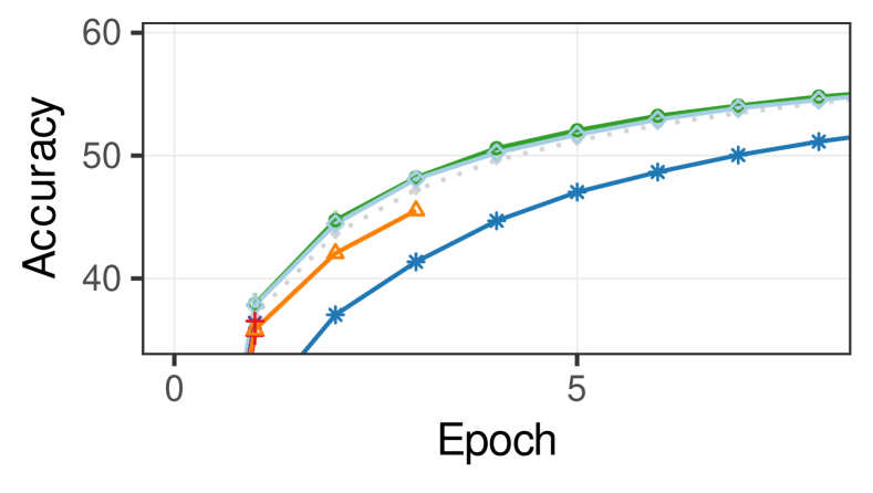
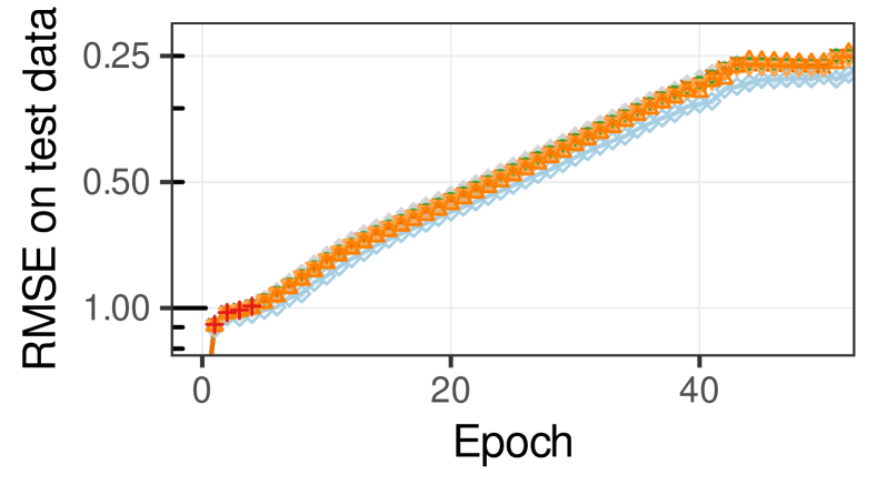
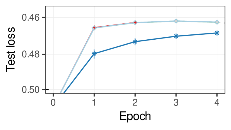
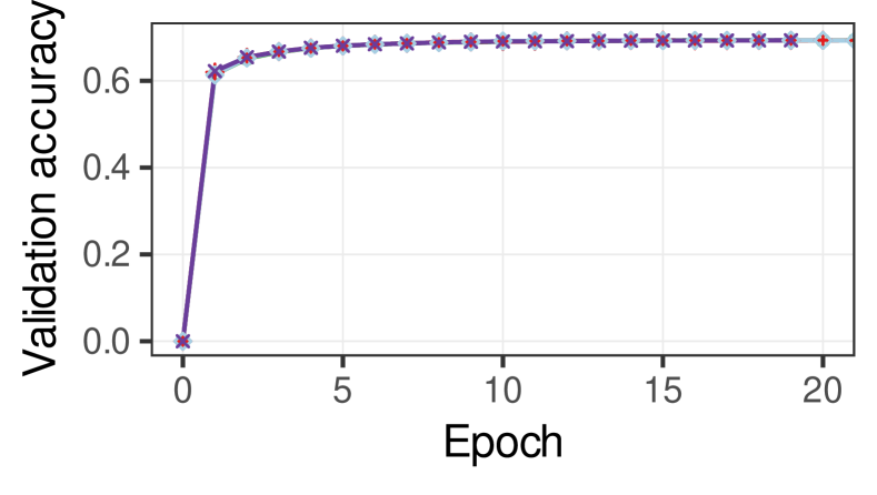
Graph neural networks. GNNs are a class of artificial neural networks that capture graph dependencies via message passing between the nodes of the graph. This task, based on Wang et al. (Wang et al., 2019b), trains a 2-layer graph convolutional network (GCN) (Schlichtkrull et al., 2018) for the node property prediction task for the ogbn-papers100M dataset from the open graph benchmark (Hu et al., 2020), using mini-batch SGD, neighbor sampling (Hamilton et al., 2017), and AdaGrad (Duchi et al., 2011). The task ignores the provided word embedding features and instead learns node embeddings from scratch. We used an embedding dimension of $500$, a batch size of 32 (per worker), and sample $16$ neighbors per layer. We partitioned the graph to the cluster nodes using METIS (Karypis and Kumar, 1998) and report validation accuracy as model quality.

Click-through-rate prediction. CTR models are common in online advertising to evaluate ad performance. This task, based on Wang et al. (Wang et al., 2022), trains the Wide & Deep model (Cheng et al., 2016) (one of the most common CTR models) with mini-batch SGD and AdaGrad (Duchi et al., 2011) on the Criteo Kaggle dataset. We used an embedding dimension of $128$, a batch size of $128$ (per worker), and a learning rate of $0.0001$. As Wang et al. (Wang et al., 2017), we used the first 6 days of data as the training data, and randomly split the 7th day into validation and test data sets. We randomly partitioned the training data to the nodes and report the test loss as model quality.

(a) CTR: raw

(b) GNN: raw

(c) CTR: effective

(d) GNN: effective

Figure 13. Further scalability results (logarithmic axes). Raw (a-b) and effective speedup (c-d).

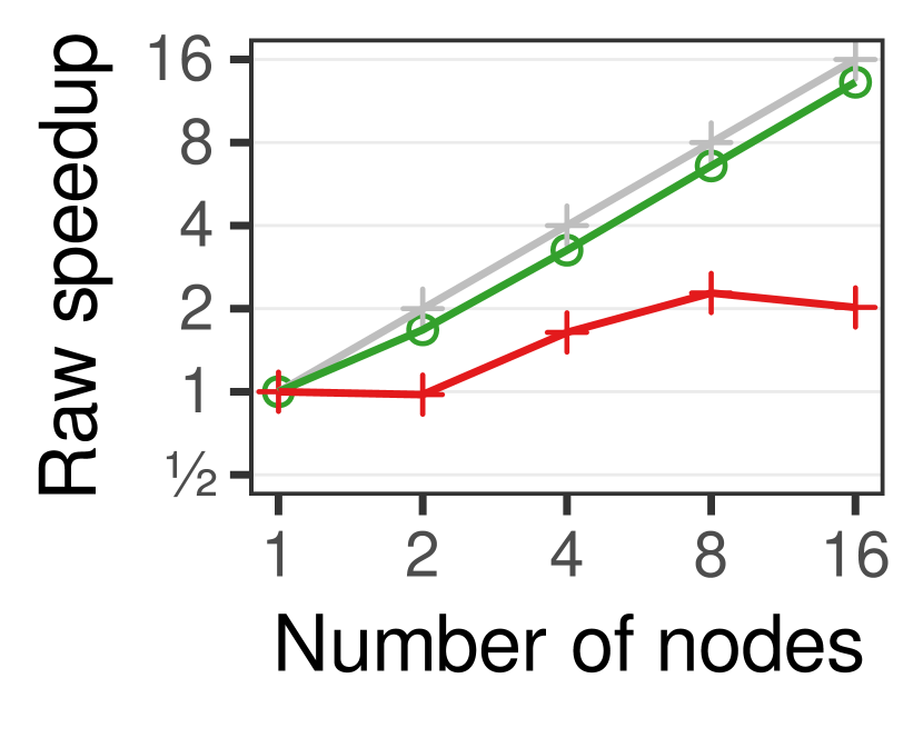
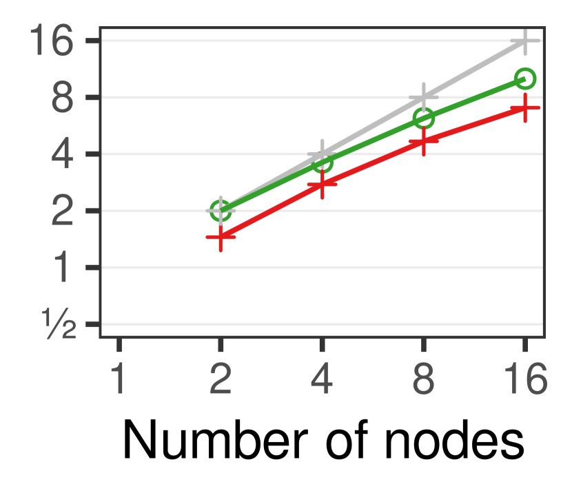
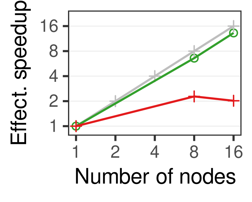
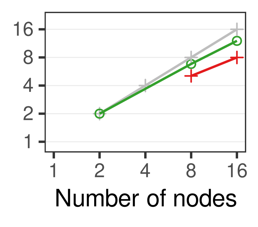
Negative sampling. For the tasks that use negative sampling (KGE and WV), we used local sampling in NuPS and AdaPM. In static parameter partitioning, we used independent sampling, as local sampling provides poor sampling quality when combined with static parameter partitioning (Renz-Wieland et al., 2022).

Default intent signal offset. In AdaPM, we used arbitrary large values for the intent signal offset ($1000$ data points in KGE, $2000$ sentences in WV, and $10\,000$ data points in MF, $100$ batches in DLRS and GNN). When chosen large enough, the offset did not affect AdaPM’s performance (see Section 5.8).

(a) KGE: run time

(b) WV: run time

(c) MF: run time

(d) KGE: quality

(e) WV: quality

(f) MF: quality

Figure 14. The effect of adaptive action timing on epoch run time (a-c) and model quality after one epoch (d-f).

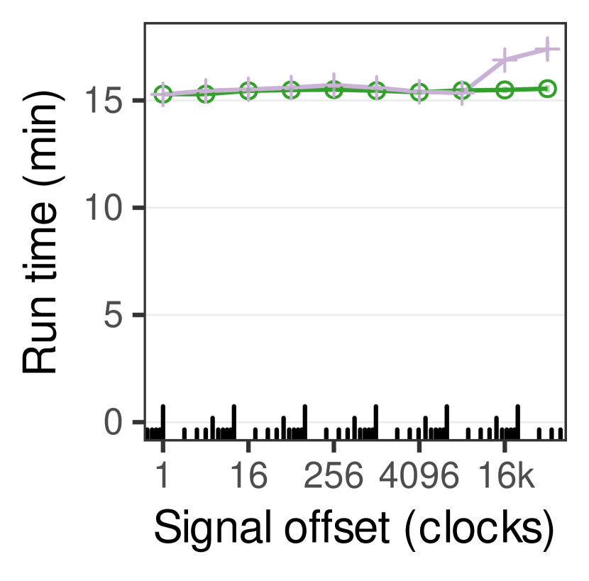
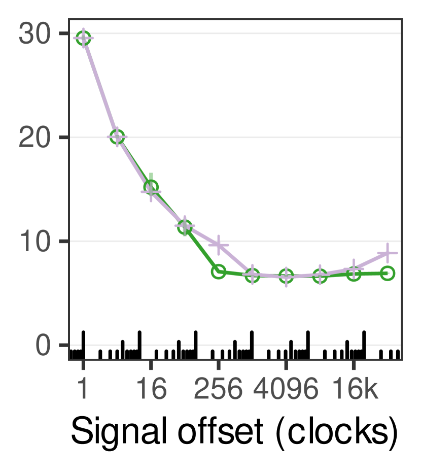
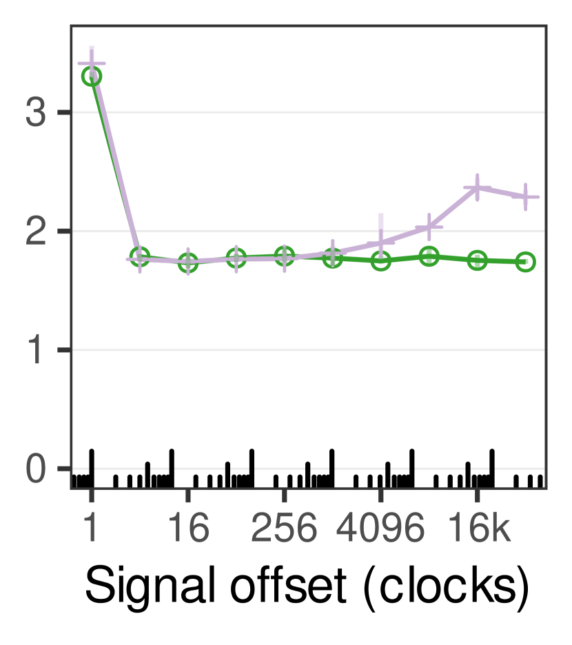
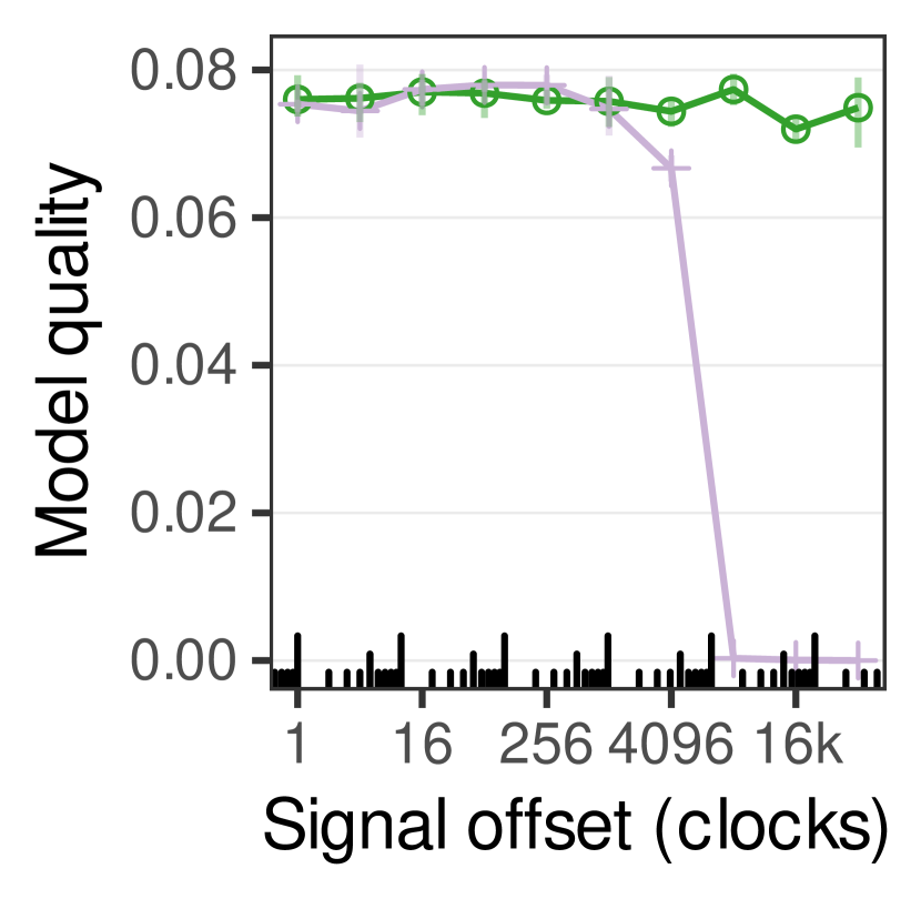
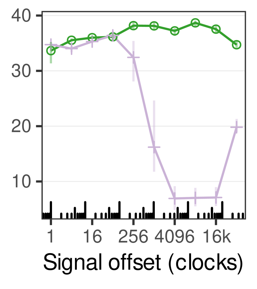
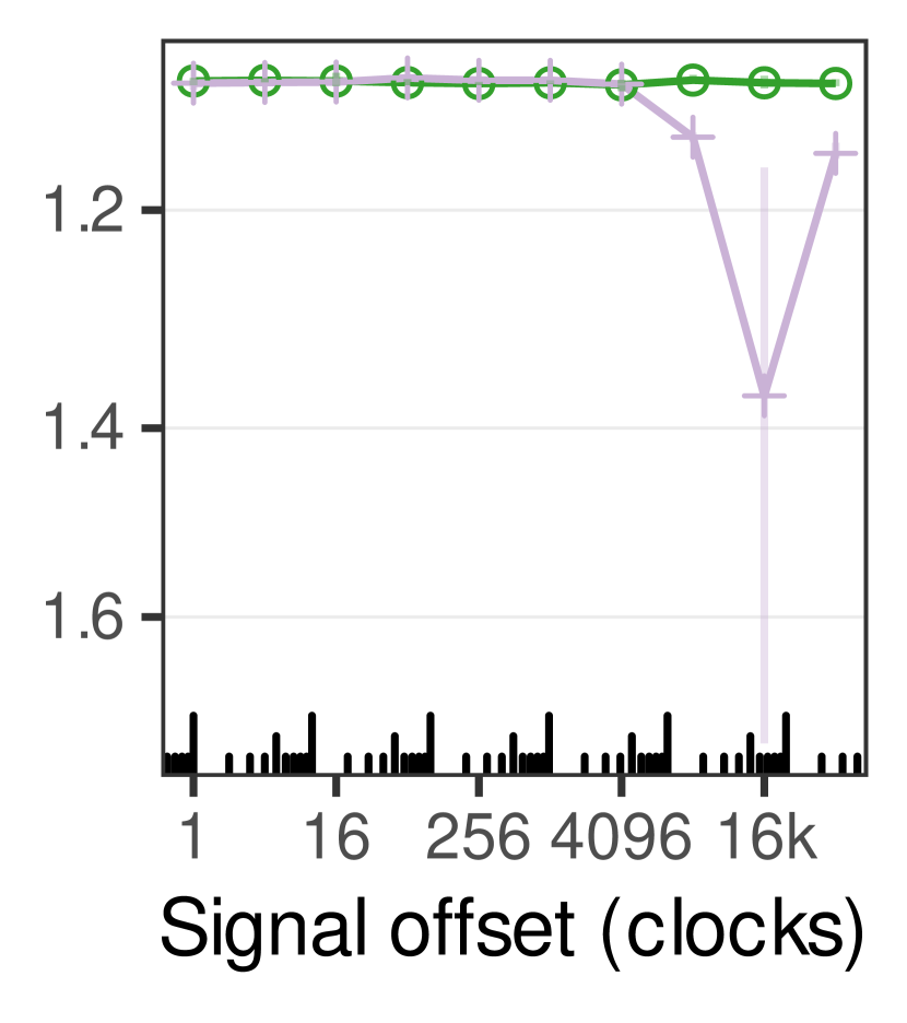
Appendix D NuPS Configurations

The main performance hyperparameters of NuPS are (i) choosing the management techniques for each parameter and (ii) specifying a relocation offset. We generated five configurations quasi-randomly using the Sobol sequence implementation of Ax (Bakshy et al., 2018). For choosing techniques, we narrowed the search range using the NuPS heuristic proposed by Renz-Wieland et al. (Renz-Wieland et al., 2022) (based on pre-computed dataset frequency statistics) for each task. We generated one set of configurations that replicate 0.01x–100x as many parameters (because Renz-Wieland et al. (Renz-Wieland et al., 2022) report that up to 64x deviations from the heuristic were beneficial). For the relocation offset, we set the search space to 1–1000 as we found that offsets of up to 512 can be beneficial (see Section 5.8). We use the same set of configurations for the three tasks. We provide more details on the search and the exact configurations online.

(a) Hot spot parameter (most frequent parameter)

(b) Hot spot parameter (99.997% frequency quantile)

(c) Hot spot parameter (99.991% frequency quantile)

(d) Frequent parameter (99.95% frequency quantile)

(e) Typical parameter (median frequency)

Figure 15. Parameter management for selected parameters in the KGE task. Each row corresponds to one of 8 nodes. The red boxes indicate two short-lived replicas.

Appendix E AdaPM in Action (Figure 15)

AdaPM decides dynamically and automatically between relocation and replication. To explore how AdaPM actually manages parameters, we traced AdaPM’s parameter management. Figure 15 depicts parameter management for selected parameters during the first half of the first epoch of KGE training on 8 nodes. AdaPM managed extreme hot spots and extreme cold spots the same way a multi-technique PS does, but used more efficient approaches for parameters between the extremes.

The extremes. NuPS decides statically how to manage a parameter. The NuPS heuristic would use static full replication for the first three depicted parameters (Figures 15(a), and 15(b), and 15(c)) and relocation for the others. AdaPM ended up managing the two extremes—i.e., the extreme hot spot (Figure 15(a)) and the rarely accessed parameter (Figure 15(e))—as NuPS would.

Between the extremes. For the parameters between these two extremes, AdaPM took more fine-grained approaches than NuPS. For example, for the parameter in Figure 15(b), AdaPM maintained replicas exactly while they were needed. Concretely, the gray areas in Figures 15(b) and 15(c) indicate periods in which AdaPM communicates less than NuPS: in contrast to AdaPM, NuPS would maintain replicas during these periods. For the parameter in Figure 15(d), AdaPM created (short-lived) replicas whenever multiple nodes accessed this parameter concurrently. These short-lived replicas are barely visible in the figure, so we highlighted two of them with red boxes. The short-term replicas prevented workers from having to access the parameter remotely. In contrast, NuPS would manage this parameter exclusively by relocation, such that workers are slowed down by remote parameter accesses.

References

- (1)
- Abadi et al. (2016) Martín Abadi, Paul Barham, Jianmin Chen, Zhifeng Chen, Andy Davis, Jeffrey Dean, Matthieu Devin, Sanjay Ghemawat, Geoffrey Irving, Michael Isard, Manjunath Kudlur, Josh Levenberg, Rajat Monga, Sherry Moore, Derek Murray, Benoit Steiner, Paul Tucker, Vijay Vasudevan, Pete Warden, Martin Wicke, Yuan Yu, and Xiaoqiang Zheng. 2016. TensorFlow: A System for Large-scale Machine Learning. In Proceedings of the 12th Conference on Operating Systems Design and Implementation (Savannah, GA, USA) (OSDI ’16). USENIX, Berkeley, CA, USA, 265–283. http://dl.acm.org/citation.cfm?id=3026877.3026899
- Adnan et al. (2021) Muhammad Adnan, Yassaman Ebrahimzadeh Maboud, Divya Mahajan, and Prashant J. Nair. 2021. Accelerating Recommendation System Training by Leveraging Popular Choices. PVLDB 15, 1 (Sept. 2021), 127–140. https://doi.org/10.14778/3485450.3485462
- Ahmed et al. (2012) Amr Ahmed, Moahmed Aly, Joseph Gonzalez, Shravan Narayanamurthy, and Alexander Smola. 2012. Scalable Inference in Latent Variable Models. In Proceedings of the 5th ACM International Conference on Web Search and Data Mining (Seattle, WA, USA) (WSDM ’12). ACM, New York, NY, USA, 123–132. https://doi.org/10.1145/2124295.2124312
- Bakshy et al. (2018) Eytan Bakshy, Lili Dworkin, Brian Karrer, Konstantin Kashin, Benjamin Letham, Ashwin Murthy, and Shaun Singh. 2018. AE: A domain-agnostic platform for adaptive experimentation. In Workshop on Systems for ML and Open Source Software at NeurIPS 2018.
- Balazevic et al. (2019) Ivana Balazevic, Carl Allen, and Timothy Hospedales. 2019. TuckER: Tensor Factorization for Knowledge Graph Completion. In Proceedings of the 2019 Conference on Empirical Methods in Natural Language Processing and the 9th International Joint Conference on Natural Language Processing (EMNLP-IJCNLP ’19). Association for Computational Linguistics, Hong Kong, China, 5185–5194. https://doi.org/10.18653/v1/D19-1522
- Bordes et al. (2013) Antoine Bordes, Nicolas Usunier, Alberto Garcia-Duran, Jason Weston, and Oksana Yakhnenko. 2013. Translating Embeddings for Modeling Multi-relational Data. In Advances in Neural Information Processing Systems (NeurIPS ’13). Curran Associates. https://proceedings.neurips.cc/paper/2013/file/1cecc7a77928ca8133fa24680a88d2f9-Paper.pdf
- Broscheit et al. (2020) Samuel Broscheit, Daniel Ruffinelli, Adrian Kochsiek, Patrick Betz, and Rainer Gemulla. 2020. LibKGE - A Knowledge Graph Embedding Library for Reproducible research. In Proceedings of the 2020 Conference on Empirical Methods in Natural Language Processing: System Demonstrations. Association for Computational Linguistics, Online, 165–174. https://doi.org/10.18653/v1/2020.emnlp-demos.22
- Chelba et al. (2013) Ciprian Chelba, Tomas Mikolov, Mike Schuster, Qi Ge, Thorsten Brants, and Phillipp Koehn. 2013. One Billion Word Benchmark for Measuring Progress in Statistical Language Modeling. CoRR abs/1312.3005 (2013). arXiv:1312.3005 http://arxiv.org/abs/1312.3005
- Chen et al. (2012) Po-Lung Chen, Chen-Tse Tsai, Yao-Nan Chen, Ku-Chun Chou, Chun-Liang Li, Cheng-Hao Tsai, Kuan-Wei Wu, Yu-Cheng Chou, Chung-Yi Li, Wei-Shih Lin, Shu-Hao Yu, Rong-Bing Chiu, Chieh-Yen Lin, Chien-Chih Wang, Po-Wei Wang, Wei-Lun Su, Chen-Hung Wu, Tsung-Ting Kuo, Todd G. McKenzie, Ya-Hsuan Chang, Chun-Sung Ferng, Chia-Mau Ni, Hsuan-Tien Lin, Chih-Jen Lin, and Shou-De Lin. 2012. A Linear Ensemble of Individual and Blended Models for Music Rating Prediction. In Proceedings of KDD Cup 2011 (Proceedings of Machine Learning Research, Vol. 18). PMLR, 21–60. https://proceedings.mlr.press/v18/chen12a.html
- Chen et al. (2015) Tianqi Chen, Mu Li, Yutian Li, Min Lin, Naiyan Wang, Minjie Wang, Tianjun Xiao, Bing Xu, Chiyuan Zhang, and Zheng Zhang. 2015. MXNet: A Flexible and Efficient Machine Learning Library for Heterogeneous Distributed Systems. CoRR abs/1512.01274 (2015). arXiv:1512.01274 http://arxiv.org/abs/1512.01274
- Cheng et al. (2016) Heng-Tze Cheng, Levent Koc, Jeremiah Harmsen, Tal Shaked, Tushar Chandra, Hrishi Aradhye, Glen Anderson, Greg Corrado, Wei Chai, Mustafa Ispir, Rohan Anil, Zakaria Haque, Lichan Hong, Vihan Jain, Xiaobing Liu, and Hemal Shah. 2016. Wide & Deep Learning for Recommender Systems. In Proceedings of the 1st Workshop on Deep Learning for Recommender Systems (Boston, MA, USA) (DLRS ’16). Association for Computing Machinery, New York, NY, USA, 7–10. https://doi.org/10.1145/2988450.2988454
- Dai et al. (2015) Wei Dai, Abhimanu Kumar, Jinliang Wei, Qirong Ho, Garth Gibson, and Eric P Xing. 2015. High-Performance Distributed ML at Scale through Parameter Server Consistency Models. In Proceedings of the 29th AAAI Conference on Artificial Intelligence (AAAI ’15). 79–87.
- Devlin et al. (2019) Jacob Devlin, Ming-Wei Chang, Kenton Lee, and Kristina Toutanova. 2019. BERT: Pre-training of Deep Bidirectional Transformers for Language Understanding. In Proceedings of the 2019 Conference of the North American Chapter of the Association for Computational Linguistics: Human Language Technologies (NAACL ’19). Association for Computational Linguistics, Minneapolis, Minnesota, 4171–4186. https://doi.org/10.18653/v1/N19-1423
- Duchi et al. (2011) John Duchi, Elad Hazan, and Yoram Singer. 2011. Adaptive Subgradient Methods for Online Learning and Stochastic Optimization. Journal of Machine Learning Research 12 (July 2011), 2121–2159. http://dl.acm.org/citation.cfm?id=1953048.2021068
- Guo et al. (2017) Huifeng Guo, Ruiming Tang, Yunming Ye, Zhenguo Li, and Xiuqiang He. 2017. DeepFM: A Factorization-Machine Based Neural Network for CTR Prediction. In Proceedings of the 26th International Joint Conference on Artificial Intelligence (Melbourne, Australia) (IJCAI’17). AAAI Press, 1725–1731.
- Hamilton et al. (2017) Will Hamilton, Zhitao Ying, and Jure Leskovec. 2017. Inductive Representation Learning on Large Graphs. In Advances in Neural Information Processing Systems (NeurIPS ’17), I. Guyon, U. Von Luxburg, S. Bengio, H. Wallach, R. Fergus, S. Vishwanathan, and R. Garnett (Eds.). Curran Associates. https://proceedings.neurips.cc/paper/2017/file/5dd9db5e033da9c6fb5ba83c7a7ebea9-Paper.pdf
- Ho et al. (2013) Qirong Ho, James Cipar, Henggang Cui, Jin Kyu Kim, Seunghak Lee, Phillip Gibbons, Garth Gibson, Gregory Ganger, and Eric Xing. 2013. More Effective Distributed ML via a Stale Synchronous Parallel Parameter Server. In Advances in Neural Information Processing Systems (Lake Tahoe, NV, USA) (NeurIPS ’13). Curran Associates, USA, 1223–1231. http://dl.acm.org/citation.cfm?id=2999611.2999748
- Hu et al. (2020) Weihua Hu, Matthias Fey, Marinka Zitnik, Yuxiao Dong, Hongyu Ren, Bowen Liu, Michele Catasta, and Jure Leskovec. 2020. Open Graph Benchmark: Datasets for Machine Learning on Graphs. In Advances in Neural Information Processing Systems (NeurIPS ’20), H. Larochelle, M. Ranzato, R. Hadsell, M.F. Balcan, and H. Lin (Eds.). Curran Associates, 22118–22133. https://proceedings.neurips.cc/paper/2020/file/fb60d411a5c5b72b2e7d3527cfc84fd0-Paper.pdf
- Hu et al. (2008) Yifan Hu, Yehuda Koren, and Chris Volinsky. 2008. Collaborative Filtering for Implicit Feedback Datasets. In 8th IEEE International Conference on Data Mining (ICDM ’08). 263–272. https://doi.org/10.1109/ICDM.2008.22
- Huang et al. (2018) Yuzhen Huang, Tatiana Jin, Yidi Wu, Zhenkun Cai, Xiao Yan, Fan Yang, Jinfeng Li, Yuying Guo, and James Cheng. 2018. FlexPS: Flexible Parallelism Control in Parameter Server Architecture. PVLDB 11, 5 (Jan. 2018), 566–579. https://doi.org/10.1145/3187009.3177734
- Karypis and Kumar (1998) George Karypis and Vipin Kumar. 1998. A Fast and High Quality Multilevel Scheme for Partitioning Irregular Graphs. SIAM Journal on Scientific Computing 20, 1 (1998), 359–392. https://doi.org/10.1137/S1064827595287997 arXiv:https://doi.org/10.1137/S1064827595287997
- Kim et al. (2019) Soojeong Kim, Gyeong-In Yu, Hojin Park, Sungwoo Cho, Eunji Jeong, Hyeonmin Ha, Sanha Lee, Joo Seong Jeong, and Byung-Gon Chun. 2019. Parallax: Sparsity-Aware Data Parallel Training of Deep Neural Networks. In Proceedings of the 14th European Conference on Computer Systems (Dresden, Germany) (EuroSys ’19). Association for Computing Machinery, New York, NY, USA, Article 43, 15 pages. https://doi.org/10.1145/3302424.3303957
- Kochsiek and Gemulla (2021) Adrian Kochsiek and Rainer Gemulla. 2021. Parallel Training of Knowledge Graph Embedding Models: A Comparison of Techniques. PVLDB 15, 3 (Nov. 2021), 633–645. https://doi.org/10.14778/3494124.3494144
- Koren et al. (2009) Yehuda Koren, Robert Bell, and Chris Volinsky. 2009. Matrix Factorization Techniques for Recommender Systems. Computer 42, 8 (Aug. 2009), 30–37. https://doi.org/10.1109/MC.2009.263
- LeCun et al. (1989) Y. LeCun, B. Boser, J. S. Denker, D. Henderson, R. E. Howard, W. Hubbard, and L. D. Jackel. 1989. Backpropagation Applied to Handwritten Zip Code Recognition. Neural Computation 1, 4 (Dec. 1989), 541–551. https://doi.org/10.1162/neco.1989.1.4.541
- Lerer et al. (2019) Adam Lerer, Ledell Wu, Jiajun Shen, Timothee Lacroix, Luca Wehrstedt, Abhijit Bose, and Alex Peysakhovich. 2019. PyTorch-BigGraph: A Large-scale Graph Embedding System. In Proceedings of Machine Learning and Systems (MLSys ’19). 120–131. https://proceedings.mlsys.org/paper/2019/file/e2c420d928d4bf8ce0ff2ec19b371514-Paper.pdf
- Li et al. (2014) Mu Li, David Andersen, Jun Woo Park, Alexander Smola, Amr Ahmed, Vanja Josifovski, James Long, Eugene Shekita, and Bor-Yiing Su. 2014. Scaling Distributed Machine Learning with the Parameter Server. In Proceedings of the 11th Conference on Operating Systems Design and Implementation (Broomfield, CO, USA) (OSDI ’14). USENIX, Berkeley, CA, USA, 583–598. http://dl.acm.org/citation.cfm?id=2685048.2685095
- Li et al. (2020) Shen Li, Yanli Zhao, Rohan Varma, Omkar Salpekar, Pieter Noordhuis, Teng Li, Adam Paszke, Jeff Smith, Brian Vaughan, Pritam Damania, and Soumith Chintala. 2020. PyTorch Distributed: Experiences on Accelerating Data Parallel Training. PVLDB 13, 12 (Aug. 2020), 3005–3018. https://doi.org/10.14778/3415478.3415530
- Lian et al. (2015) Xiangru Lian, Yijun Huang, Yuncheng Li, and Ji Liu. 2015. Asynchronous Parallel Stochastic Gradient for Nonconvex Optimization. In Advances in Neural Information Processing Systems (Montreal, Canada) (NeurIPS ’15). MIT Press, Cambridge, MA, USA, 2737–2745.
- Liu et al. (2017) Hanxiao Liu, Yuexin Wu, and Yiming Yang. 2017. Analogical Inference for Multi-relational Embeddings. In Proceedings of the 34th International Conference on Machine Learning (ICML ’17). PMLR, 2168–2178. http://proceedings.mlr.press/v70/liu17d.html
- Liu et al. (2018) Xiaodong Liu, Yelong Shen, Kevin Duh, and Jianfeng Gao. 2018. Stochastic Answer Networks for Machine Reading Comprehension. In Proceedings of the 56th Annual Meeting of the Association for Computational Linguistics (ACL ’18). Association for Computational Linguistics, Melbourne, Australia, 1694–1704. https://doi.org/10.18653/v1/P18-1157
- Miao et al. (2021) Xupeng Miao, Hailin Zhang, Yining Shi, Xiaonan Nie, Zhi Yang, Yangyu Tao, and Bin Cui. 2021. HET: Scaling out Huge Embedding Model Training via Cache-Enabled Distributed Framework. PVLDB 15, 2 (Oct. 2021), 312–320. https://doi.org/10.14778/3489496.3489511
- Mikolov et al. (2013) Tomas Mikolov, Kai Chen, Greg Corrado, and Jeffrey Dean. 2013. Efficient Estimation of Word Representations in Vector Space. In Proceedings of the 1st International Conference on Learning Representations (ICLR ’13). http://arxiv.org/abs/1301.3781
- Min et al. (2021) Seung Won Min, Kun Wu, Sitao Huang, Mert Hidayetoğlu, Jinjun Xiong, Eiman Ebrahimi, Deming Chen, and Wen-mei Hwu. 2021. Large Graph Convolutional Network Training with GPU-Oriented Data Communication Architecture. PVLDB 14, 11 (Oct. 2021), 2087–2100. https://doi.org/10.14778/3476249.3476264
- Nickel et al. (2016) Maximilian Nickel, Kevin Murphy, Volker Tresp, and Evgeniy Gabrilovich. 2016. A Review of Relational Machine Learning for Knowledge Graphs. Proc. IEEE 104, 1 (Jan 2016), 11–33. https://doi.org/10.1109/JPROC.2015.2483592
- Nickel et al. (2011) Maximilian Nickel, Volker Tresp, and Hans-Peter Kriegel. 2011. A Three-way Model for Collective Learning on Multi-relational Data. In Proceedings of the 28th International Conference on Machine Learning (Bellevue, Washington, USA) (ICML ’11). Omnipress, USA, 809–816. http://dl.acm.org/citation.cfm?id=3104482.3104584
- Paszke et al. (2019) Adam Paszke, Sam Gross, Francisco Massa, Adam Lerer, James Bradbury, Gregory Chanan, Trevor Killeen, Zeming Lin, Natalia Gimelshein, Luca Antiga, Alban Desmaison, Andreas Köpf, Edward Yang, Zach DeVito, Martin Raison, Alykhan Tejani, Sasank Chilamkurthy, Benoit Steiner, Lu Fang, Junjie Bai, and Soumith Chintala. 2019. PyTorch: An Imperative Style, High-Performance Deep Learning Library. In Advances in Neural Information Processing Systems (NeurIPS ’19). Curran Associates, Red Hook, NY, USA, Article 721, 12 pages.
- Peng et al. (2022) Jingshu Peng, Zhao Chen, Yingxia Shao, Yanyan Shen, Lei Chen, and Jiannong Cao. 2022. Sancus: Staleness-Aware Communication-Avoiding Full-Graph Decentralized Training in Large-Scale Graph Neural Networks. PVLDB 15, 9 (May 2022), 1937–1950. https://doi.org/10.14778/3538598.3538614
- Pennington et al. (2014) Jeffrey Pennington, Richard Socher, and Christopher Manning. 2014. GloVe: Global Vectors for Word Representation. In Proceedings of the 2014 Conference on Empirical Methods in Natural Language Processing (EMNLP ’14). Association for Computational Linguistics, Doha, Qatar, 1532–1543. https://doi.org/10.3115/v1/D14-1162
- Peters et al. (2018) Matthew Peters, Mark Neumann, Mohit Iyyer, Matt Gardner, Christopher Clark, Kenton Lee, and Luke Zettlemoyer. 2018. Deep Contextualized Word Representations. In Proceedings of the 2018 Conference of the North American Chapter of the Association for Computational Linguistics: Human Language Technologies (NAACL ’18). Association for Computational Linguistics, New Orleans, Louisiana, 2227–2237. https://doi.org/10.18653/v1/N18-1202
- Řehůřek and Sojka (2010) Radim Řehůřek and Petr Sojka. 2010. Software Framework for Topic Modelling with Large Corpora. In Proceedings of the LREC 2010 Workshop on New Challenges for NLP Frameworks (LREC ’10). ELRA, Valletta, Malta, 45–50. http://is.muni.cz/publication/884893/en.
- Renz-Wieland et al. (2022) Alexander Renz-Wieland, Rainer Gemulla, Zoi Kaoudi, and Volker Markl. 2022. NuPS: A Parameter Server for Machine Learning with Non-Uniform Parameter Access. In Proceedings of the 2022 ACM International Conference on Management of Data (Philadelphia, Pennsylvania, USA) (SIGMOD ’22). Association for Computing Machinery, New York, NY, USA.
- Renz-Wieland et al. (2020) Alexander Renz-Wieland, Rainer Gemulla, Steffen Zeuch, and Volker Markl. 2020. Dynamic Parameter Allocation in Parameter Servers. PVLDB 13, 12 (July 2020), 1877–1890. https://doi.org/10.14778/3407790.3407796
- Ruffinelli et al. (2020) Daniel Ruffinelli, Samuel Broscheit, and Rainer Gemulla. 2020. You CAN Teach an Old Dog New Tricks! On Training Knowledge Graph Embeddings. In Proceedings of the 8th International Conference on Learning Representations (ICLR ’20). https://openreview.net/forum?id=BkxSmlBFvr
- Schlichtkrull et al. (2018) Michael Schlichtkrull, Thomas N. Kipf, Peter Bloem, Rianne van den Berg, Ivan Titov, and Max Welling. 2018. Modeling Relational Data with Graph Convolutional Networks. In The Semantic Web (ESWC ’18). Springer International Publishing, Cham, 593–607.
- Sergeev and Balso (2018) Alexander Sergeev and Mike Del Balso. 2018. Horovod: Fast and easy distributed deep learning in TensorFlow. CoRR abs/1802.05799 (2018). arXiv:1802.05799 http://arxiv.org/abs/1802.05799
- Shang et al. (2019) Chao Shang, Yun Tang, Jing Huang, Jinbo Bi, Xiaodong He, and Bowen Zhou. 2019. End-to-End Structure-Aware Convolutional Networks for Knowledge Base Completion. In Proceedings of the 33rd AAAI Conference on Artificial Intelligence (AAAI ’19). 3060–3067. https://doi.org/10.1609/aaai.v33i01.33013060
- Smola and Narayanamurthy (2010) Alexander Smola and Shravan Narayanamurthy. 2010. An Architecture for Parallel Topic Models. PVLDB 3, 1-2 (Sept. 2010), 703–710. https://doi.org/10.14778/1920841.1920931
- Socher et al. (2013) Richard Socher, John Bauer, Christopher Manning, and Andrew Ng. 2013. Parsing with Compositional Vector Grammars. In Proceedings of the 51st Annual Meeting of the Association for Computational Linguistics (ACL ’13). Association for Computational Linguistics, Sofia, Bulgaria, 455–465. https://www.aclweb.org/anthology/P13-1045
- Teflioudi et al. (2012) Christina Teflioudi, Faraz Makari, and Rainer Gemulla. 2012. Distributed Matrix Completion. In 12th IEEE International Conference on Data Mining (ICDM ’12). 655–664. https://doi.org/10.1109/ICDM.2012.120
- Trouillon et al. (2016) Théo Trouillon, Johannes Welbl, Sebastian Riedel, Éric Gaussier, and Guillaume Bouchard. 2016. Complex Embeddings for Simple Link Prediction. In Proceedings of the 33rd International Conference on Machine Learning (New York, NY, USA) (ICML ’16). JMLR.org, 2071–2080. http://dl.acm.org/citation.cfm?id=3045390.3045609
- van Steen and Tanenbaum (2017) Maarten van Steen and Andrew Tanenbaum. 2017. Distributed Systems (3rd ed.).
- Vashishth et al. (2020) Shikhar Vashishth, Soumya Sanyal, Vikram Nitin, and Partha Talukdar. 2020. Composition-based Multi-Relational Graph Convolutional Networks. In Proceedings of the 8th International Conference on Learning Representations (ICLR ’20). https://openreview.net/forum?id=BylA_C4tPr
- Waleffe et al. (2022) Roger Waleffe, Jason Mohoney, Theodoros Rekatsinas, and Shivaram Venkataraman. 2022. Marius++: Large-Scale Training of Graph Neural Networks on a Single Machine. CoRR abs/2202.02365 (2022). arXiv:2202.02365 https://arxiv.org/abs/2202.02365
- Wang et al. (2019b) Minjie Wang, Lingfan Yu, Da Zheng, Quan Gan, Yu Gai, Zihao Ye, Mufei Li, Jinjing Zhou, Qi Huang, Chao Ma, Ziyue Huang, Qipeng Guo, Hao Zhang, Haibin Lin, Junbo Zhao, Jinyang Li, Alexander J. Smola, and Zheng Zhang. 2019b. Deep Graph Library: Towards Efficient and Scalable Deep Learning on Graphs. CoRR abs/1909.01315 (2019). arXiv:1909.01315 http://arxiv.org/abs/1909.01315
- Wang et al. (2017) Ruoxi Wang, Bin Fu, Gang Fu, and Mingliang Wang. 2017. Deep & Cross Network for Ad Click Predictions. In Proceedings of the ADKDD’17 (Halifax, NS, Canada) (ADKDD’17). Association for Computing Machinery, New York, NY, USA, Article 12, 7 pages. https://doi.org/10.1145/3124749.3124754
- Wang et al. (2019a) Xiaozhi Wang, Tianyu Gao, Zhaocheng Zhu, Zhiyuan Liu, Juanzi Li, and Jian Tang. 2019a. KEPLER: A Unified Model for Knowledge Embedding and Pre-trained Language Representation. CoRR abs/1911.06136 (2019). arXiv:1911.06136 http://arxiv.org/abs/1911.06136
- Wang et al. (2022) Zehuan Wang, Yingcan Wei, Minseok Lee, Matthias Langer, Fan Yu, Jie Liu, Shijie Liu, Daniel G. Abel, Xu Guo, Jianbing Dong, Ji Shi, and Kunlun Li. 2022. Merlin HugeCTR: GPU-Accelerated Recommender System Training and Inference. In Proceedings of the 16th ACM Conference on Recommender Systems (Seattle, WA, USA) (RecSys ’22). Association for Computing Machinery, New York, NY, USA, 534–537. https://doi.org/10.1145/3523227.3547405
- Wei et al. (2015) Jinliang Wei, Wei Dai, Aurick Qiao, Qirong Ho, Henggang Cui, Gregory R. Ganger, Phillip B. Gibbons, Garth A. Gibson, and Eric P. Xing. 2015. Managed communication and consistency for fast data-parallel iterative analytics. In Proceedings of the Sixth ACM Symposium on Cloud Computing (SoCC). 381–394.
- Xing et al. (2015) Eric Xing, Qirong Ho, Wei Dai, Jin-Kyu Kim, Jinliang Wei, Seunghak Lee, Xun Zheng, Pengtao Xie, Abhimanu Kumar, and Yaoliang Yu. 2015. Petuum: A New Platform for Distributed Machine Learning on Big Data. In Proceedings of the 21th ACM SIGKDD International Conference on Knowledge Discovery and Data Mining (Sydney, NSW, Australia) (KDD ’15). ACM, New York, NY, USA, 1335–1344. https://doi.org/10.1145/2783258.2783323
- Zhao et al. (2020) Weijie Zhao, Deping Xie, Ronglai Jia, Yulei Qian, Ruiquan Ding, Mingming Sun, and Ping Li. 2020. Distributed Hierarchical GPU Parameter Server for Massive Scale Deep Learning Ads Systems. In Proceedings of Machine Learning and Systems (MLSys ’20). 412–428. https://proceedings.mlsys.org/paper/2020/file/f7e6c85504ce6e82442c770f7c8606f0-Paper.pdf
- Zheng et al. (2021) Qiming Zheng, Quan Chen, Kaihao Bai, Huifeng Guo, Yong Gao, Xiuqiang He, and Minyi Guo. 2021. BiPS: Hotness-aware Bi-tier Parameter Synchronization for Recommendation Models. In 35th IEEE International Parallel and Distributed Processing Symposium (ISDPS ’21). IEEE, 609–618. https://doi.org/10.1109/IPDPS49936.2021.00069
- Zheng et al. (2022) Zangwei Zheng, Pengtai Xu, Xuan Zou, Da Tang, Zhen Li, Chenguang Xi, Peng Wu, Leqi Zou, Yijie Zhu, Ming Chen, Xiangzhuo Ding, Fuzhao Xue, Ziheng Qing, Youlong Cheng, and Yang You. 2022. CowClip: Reducing CTR Prediction Model Training Time from 12 hours to 10 minutes on 1 GPU. CoRR abs/2204.06240 (2022). https://doi.org/10.48550/arXiv.2204.06240 arXiv:2204.06240
- Zhou et al. (2018) Guorui Zhou, Xiaoqiang Zhu, Chenru Song, Ying Fan, Han Zhu, Xiao Ma, Yanghui Yan, Junqi Jin, Han Li, and Kun Gai. 2018. Deep Interest Network for Click-Through Rate Prediction. In Proceedings of the 24th ACM SIGKDD International Conference on Knowledge Discovery and Data Mining (London, United Kingdom) (KDD ’18). Association for Computing Machinery, New York, NY, USA, 1059–1068. https://doi.org/10.1145/3219819.3219823
- Zhu et al. (2019) Rong Zhu, Kun Zhao, Hongxia Yang, Wei Lin, Chang Zhou, Baole Ai, Yong Li, and Jingren Zhou. 2019. AliGraph: A Comprehensive Graph Neural Network Platform. PVLDB 12, 12 (Aug. 2019), 2094–2105. https://doi.org/10.14778/3352063.3352127