Quadratic models for understanding neural network dynamics

Libin Zhu     Chaoyue Liu     Adityanarayanan Radhakrishnan     Mikhail Belkin
Department of Computer Science & Halicioğlu Data Science Institute, University of California, San Diego. E-mail: l5zhu@ucsd.eduHalicioğlu Data Science Institute, University of California, San Diego. E-mail: ch1212@ucsd.eduMassachusetts Institute of Technology & Broad Institute of MIT and Harvard. E-mail: aradha@mit.eduHalicioğlu Data Science Institute & Department of Computer Science, University of California, San Diego. E-mail: mbelkin@ucsd.edu
Abstract

While neural networks can be approximated by linear models as their width increases, certain properties of wide neural networks cannot be captured by linear models. In this work we show that recently proposed Neural Quadratic Models can exhibit the “catapult phase” [15] that arises when training such models with large learning rates. We then empirically show that the behaviour of neural quadratic models parallels that of neural networks in generalization, especially in the catapult phase regime. Our analysis further demonstrates that quadratic models can be an effective tool for analysis of neural networks.

1 Introduction

A recent remarkable finding on neural networks, originating from [9] and termed as the “transition to linearity” [16], is that, as network width goes to infinity, such models become linear functions in the parameter space. Thus, a linear (in parameters) model can be built to accurately approximate wide neural networks under certain conditions. While this finding has helped improve our understanding of trained neural networks [4, 20, 29, 18, 11, 3], not all properties of finite width neural networks can be understood in terms of linear models, as is shown in several recent works [27, 21, 17, 6]. In this work, we show that properties of finitely wide neural networks in optimization and generalization that cannot be captured by linear models are, in fact, manifested in quadratic models.

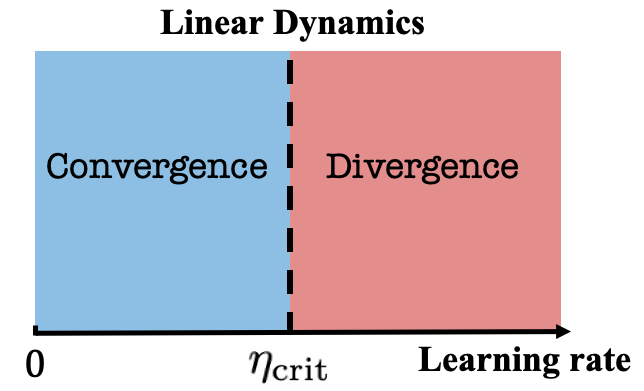
The training dynamics of linear models with respect to the choice of the learning rates111Unless stated otherwise, we always consider the setting where models are trained with squared loss using gradient descent. are well-understood [22]. Indeed, such models exhibit linear training dynamics, i.e., there exists a critical learning rate, ηcritsubscript𝜂crit{\eta_{\mathrm{crit}}}, such that the loss converges monotonically if and only if the learning rate is smaller than ηcritsubscript𝜂crit{\eta_{\mathrm{crit}}} (see Figure 1a).

Refer to caption
(a)
Refer to caption
(b)
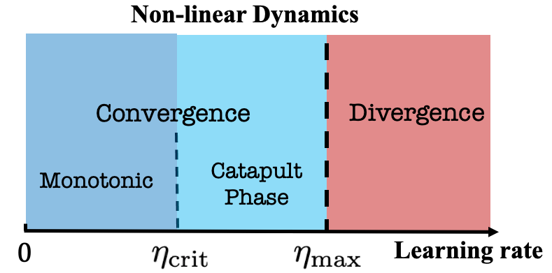
Figure 1: Optimization dynamics for linear and non-linear models based on choice of learning rate. (a) Linear models either converge monotonically if learning rate is less than ηcritsubscript𝜂crit{\eta_{\mathrm{crit}}} and diverge otherwise. (b) Unlike linear models, finitely wide neural networks and NQMs Eq. (2) (or general quadratic models Eq. (3)) can additionally observe a catapult phase when ηcrit<η<ηmaxsubscript𝜂crit𝜂subscript𝜂max{\eta_{\mathrm{crit}}}<\eta<{\eta_{\mathrm{max}}}.
Refer to caption
(a) Optimization dynamics for f𝑓f (wide neural networks): linear dynamics and catapult dynamics.
Refer to caption
(b) Generalization performance for f𝑓f, flinsubscript𝑓linf_{{{\mathrm{lin}}}} and fquadsubscript𝑓quadf_{{\mathrm{quad}}}.
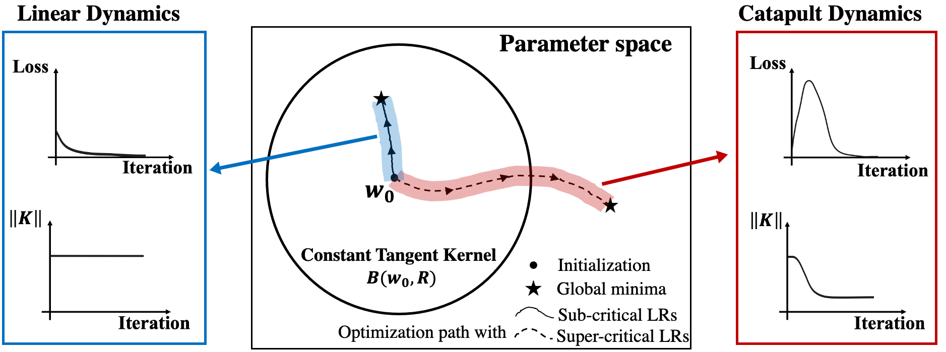
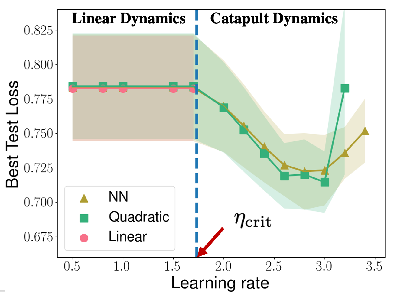
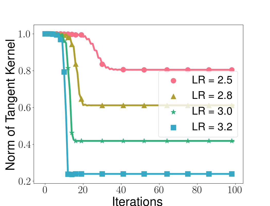
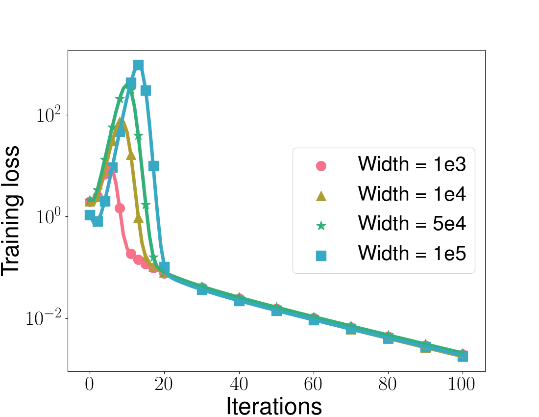
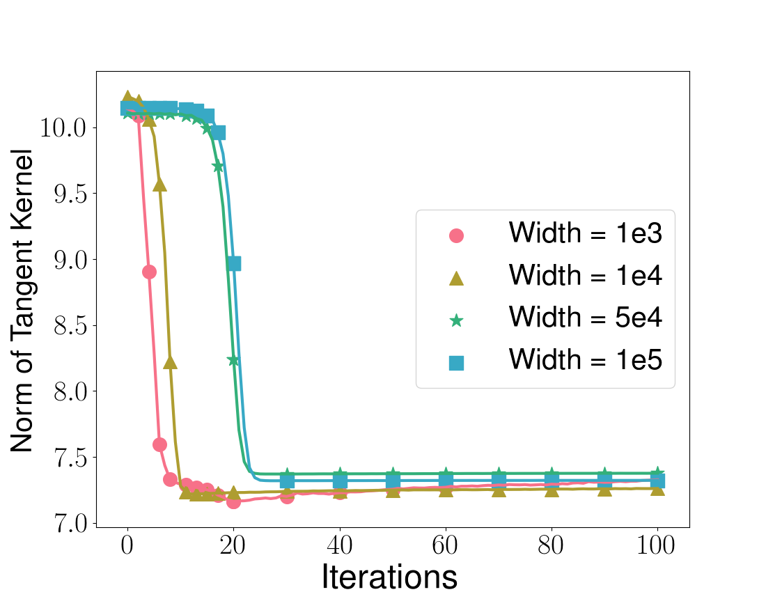
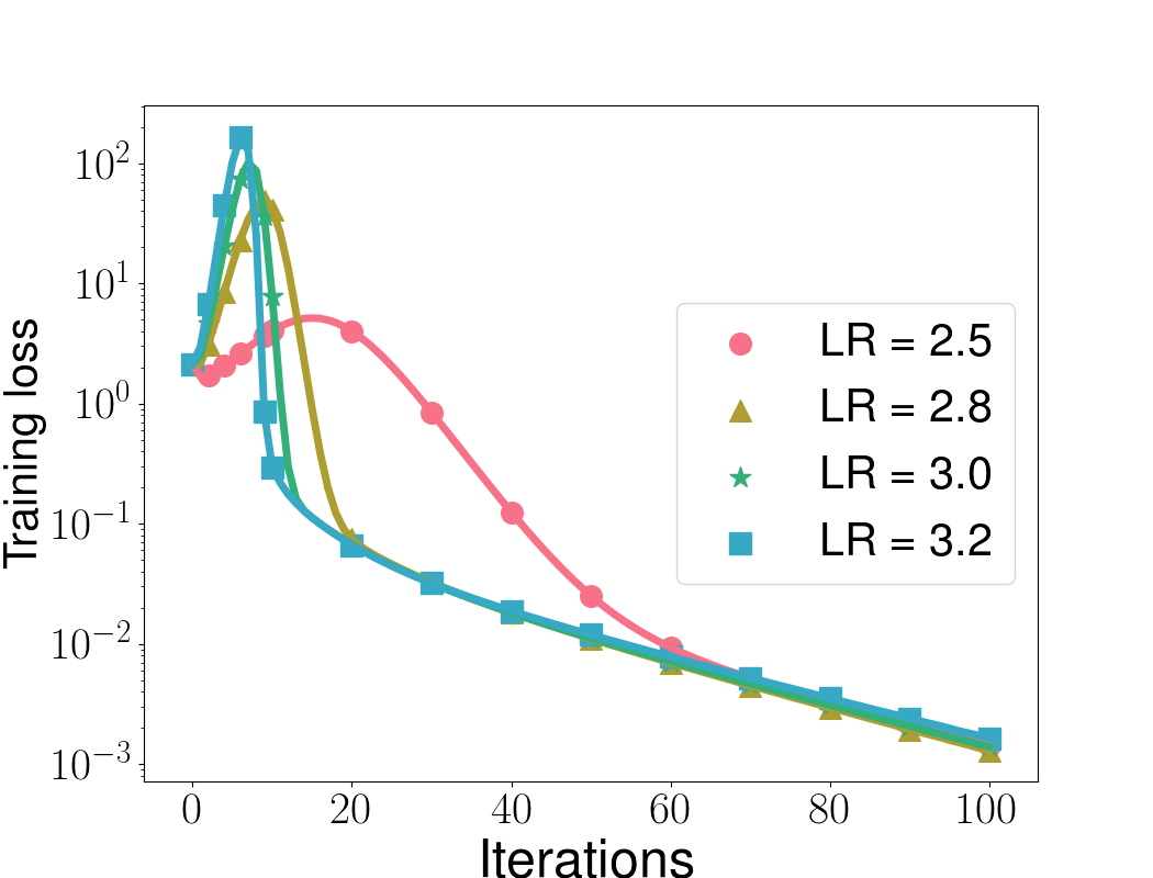
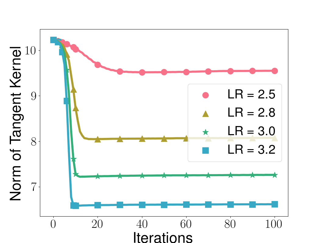
Figure 2: (a) Optimization dynamics of wide neural networks with sub-critical and super-critical learning rates. With sub-critical learning rates (0<η<ηcrit)0<\eta<{\eta_{\mathrm{crit}}}), the tangent kernel of wide neural networks is nearly constant during training, and the loss decreases monotonically. The whole optimization path is contained in the ball B(𝐰0,R):={𝐰:𝐰𝐰0R}assign𝐵subscript𝐰0𝑅conditional-set𝐰norm𝐰subscript𝐰0𝑅B({\mathbf{w}}_{0},R):=\{{\mathbf{w}}:\|{\mathbf{w}}-{\mathbf{w}}_{0}\|\leq R\} with a finite radius R𝑅R. With super-critical learning rates (ηcrit<η<ηmax){\eta_{\mathrm{crit}}}<\eta<{\eta_{\mathrm{max}}}), the catapult phase happens: the loss first increases and then decreases, along with a decrease of the norm of the tangent kernel . The optimization path goes beyond the finite radius ball. (b) Test loss of fquadsubscript𝑓quadf_{{\mathrm{quad}}}, f𝑓f and flinsubscript𝑓linf_{{{\mathrm{lin}}}} plotted against different learning rates. With sub-critical learning rates, all three models have nearly identical test loss for any sub-critical learning rate. With super-critical learning rates, f𝑓f and fquadsubscript𝑓quadf_{{\mathrm{quad}}} have smaller best test loss than the one with sub-critical learning rates. Experimental details are in Appendix N.5.

Recent work [14] showed that the training dynamics of a wide neural network f(𝐰;𝒙)𝑓𝐰𝒙f({\mathbf{w}};{\boldsymbol{x}}) can be accurately approximated by that of a linear model flin(𝐰;𝒙)subscript𝑓lin𝐰𝒙f_{{{\mathrm{lin}}}}({\mathbf{w}};{\boldsymbol{x}}):

flin(𝐰;𝒙)=f(𝐰0;𝒙)+(𝐰𝐰0)Tf(𝐰0;𝒙),subscript𝑓lin𝐰𝒙𝑓subscript𝐰0𝒙superscript𝐰subscript𝐰0𝑇𝑓subscript𝐰0𝒙\displaystyle f_{\mathrm{lin}}({\mathbf{w}};{\boldsymbol{x}})=f({\mathbf{w}}_{0};{\boldsymbol{x}})+({\mathbf{w}}-{\mathbf{w}}_{0})^{T}\nabla f({\mathbf{w}}_{0};{\boldsymbol{x}}), (1)

where f(𝐰0;𝒙)𝑓subscript𝐰0𝒙\nabla f({\mathbf{w}}_{0};{\boldsymbol{x}}) denotes the gradient222For non-differentiable functions, e.g. neural networks with ReLU activation functions, we define the gradient based on the update rule used in practice. Similarly, we use Hfsubscript𝐻𝑓H_{f} to denote the second derivative of f𝑓f in Eq. (2). of f𝑓f with respect to trainable parameters 𝐰𝐰{\mathbf{w}} at an initial point 𝐰0subscript𝐰0{\mathbf{w}}_{0} and input sample 𝒙𝒙{\boldsymbol{x}}. This approximation holds for learning rates less than ηcrit2/f(𝐰0;𝒙)2subscript𝜂crit2superscriptnorm𝑓subscript𝐰0𝒙2{\eta_{\mathrm{crit}}}\approx 2/\|\nabla f({\mathbf{w}}_{0};{\boldsymbol{x}})\|^{2}, when the width is sufficiently large.

However, the training dynamics of finite width neural networks, f𝑓f, can sharply differ from those of linear models when using large learning rates. A striking non-linear property of wide neural networks discovered in [15] is that when the learning rate is larger than ηcritsubscript𝜂crit{\eta_{\mathrm{crit}}} but smaller than a certain maximum learning rate, ηmaxsubscript𝜂max{\eta_{\mathrm{max}}}, gradient descent still converges but experiences a “catapult phase.” Specifically, the loss initially grows exponentially and then decreases after reaching a large value, along with the decrease of the norm of tangent kernel (see Figure 2a), and therefore, such training dynamics are non-linear (see Figure 1b).

As linear models cannot exhibit such a catapult phase, under what models and conditions does this phenomenon arise? The work of [15] first observed the catapult phase phenomenon in finite width neural networks and analyzed this phenomenon for a two-layer linear neural network. However, a theoretical understanding of this phenomenon for general non-linear neural networks remains open. In this work, we utilize a quadratic model as a tool to shed light on the optimization and generalization discrepancies between finite and infinite width neural networks. We define Neural Quadratic Model (NQM) by the second order Taylor series expansion of f(𝐰;𝒙)𝑓𝐰𝒙f({\mathbf{w}};{\boldsymbol{x}}) around the point 𝐰0subscript𝐰0{\mathbf{w}}_{0}:

𝐍𝐐𝐌:fquad(𝐰)=f(𝐰0)+(𝐰𝐰0)Tf(𝐰0)+12(𝐰𝐰0)THf(𝐰0)(𝐰𝐰0).\displaystyle\vspace{-2pt}\mathbf{NQM:}~{}~{}~{}~{}f_{\mathrm{quad}}({\mathbf{w}})=f({\mathbf{w}}_{0})+({\mathbf{w}}-{\mathbf{w}}_{0})^{T}\nabla f({\mathbf{w}}_{0})+\frac{1}{2}({\mathbf{w}}-{\mathbf{w}}_{0})^{T}H_{f}({\mathbf{w}}_{0})({\mathbf{w}}-{\mathbf{w}}_{0}).\vspace{-2pt} (2)

Here in the notation we suppress the dependence on the input data 𝒙𝒙{\boldsymbol{x}}, and Hf(𝐰0)subscript𝐻𝑓subscript𝐰0H_{f}({\mathbf{w}}_{0}) is the Hessian of f𝑓f with respect to 𝐰𝐰{\mathbf{w}} evaluated at 𝐰0subscript𝐰0{\mathbf{w}}_{0}. Note that fquad(𝐰)=flin(𝐰)+12(𝐰𝐰0)THf(𝐰0)(𝐰𝐰0)subscript𝑓quad𝐰subscript𝑓lin𝐰12superscript𝐰subscript𝐰0𝑇subscript𝐻𝑓subscript𝐰0𝐰subscript𝐰0f_{\mathrm{quad}}({\mathbf{w}})=f_{\mathrm{lin}}({\mathbf{w}})+\frac{1}{2}({\mathbf{w}}-{\mathbf{w}}_{0})^{T}H_{f}({\mathbf{w}}_{0})({\mathbf{w}}-{\mathbf{w}}_{0}).

Indeed, we note that NQMs are contained in a more general class of quadratic models:

𝐆𝐞𝐧𝐞𝐫𝐚𝐥𝐐𝐮𝐚𝐝𝐫𝐚𝐭𝐢𝐜𝐌𝐨𝐝𝐞𝐥:g(𝐰;𝒙)=𝐰Tϕ(𝒙)+12γ𝐰TΣ(𝒙)𝐰,\displaystyle\mathbf{General~{}Quadratic~{}Model:}~{}~{}~{}~{}~{}~{}~{}g({\mathbf{w}};{\boldsymbol{x}})={\mathbf{w}}^{T}\phi({\boldsymbol{x}})+\frac{1}{2}\gamma{\mathbf{w}}^{T}\Sigma({\boldsymbol{x}}){\mathbf{w}}, (3)

where 𝐰𝐰{\mathbf{w}} are trainable parameters and 𝒙𝒙{\boldsymbol{x}} is input data. We discuss the optimization dynamics of such general quadratic models in Section 3.3 and show empirically that they exhibit the catapult phase phenomenon in Appendix N.4. Note that the two-layer linear network analyzed in [15] is a special case of Eq. (3), when ϕ(𝒙)=0italic-ϕ𝒙0\phi({\boldsymbol{x}})=0 (See Appendix M).

Main Contributions. We prove that NQMs, fquadsubscript𝑓quadf_{{\mathrm{quad}}}, which approximate shallow fully-connected ReLU activated neural networks, exhibit catapult phase dynamics. Specifically, we analyze the optimization dynamics of fquadsubscript𝑓quadf_{{\mathrm{quad}}} by deriving the evolution of fquadsubscript𝑓quadf_{{\mathrm{quad}}} and the tangent kernel during gradient descent with squared loss, for a single training example and multiple uni-dimensional training examples. We identify three learning rate regimes yielding different optimization dynamics for fquadsubscript𝑓quadf_{{\mathrm{quad}}}, which are (1) converging monotonically (linear dynamics); (2) converging via a catapult phase (catapult dynamics); and (3) diverging. We provide a number of experimental results corroborating our theoretical analysis (See Section 3).

We then empirically show that NQMs, for the architectures of shallow (see Figure 2b as an example) and deep networks, have better test performances when catapult dynamics happens. While this was observed for some synthetic examples of neural networks in [15], we systematically demonstrate the improved generalization of NQMs across a range of experimental settings. Namely, we consider fully-connected and convolutional neural networks with ReLU and other activation functions trained with GD/SGD on multiple vision, speech and text datatsets (See Section 4).

To the best of our knowledge, our work is the first to analyze the non-linear wide neural networks in the catapult regime through the perspective of the quadratic approximation. While NQMs (or quadratic models) were proposed and analyzed in [24], our work focuses on the properties of NQMs in the large learning rate regime, which has not been discussed in [24]. Similarly, the following related works did not study catapult dynamics. [8] analyzed higher order approximations to neural networks under gradient flow (infinitesimal learning rates). [1] studied different quadratic models with randomized second order terms and [28] considered the loss in the quadratic form, where no catapult phase happens.

Discontinuity in dynamics transition.

In the ball B(𝐰0,R):={𝐰:𝐰𝐰0R}assign𝐵subscript𝐰0𝑅conditional-set𝐰norm𝐰subscript𝐰0𝑅B({\mathbf{w}}_{0},R):=\{{\mathbf{w}}:\|{\mathbf{w}}-{\mathbf{w}}_{0}\|\leq R\} with constant radius R>0𝑅0R>0, the transition to linearity of a wide neural network (with linear output layer) is continuous in the network width m𝑚m. That is, the deviation from the network function to its linear approximation within the ball can be continuously controlled by the Hessian of the network function, i.e. Hfsubscript𝐻𝑓H_{f}, which scales with m𝑚m [16]:

f(𝐰)flin(𝐰)sup𝐰B(𝐰0,R)Hf(𝐰)R2=O~(1/m).norm𝑓𝐰subscript𝑓lin𝐰subscriptsupremum𝐰𝐵subscript𝐰0𝑅normsubscript𝐻𝑓𝐰superscript𝑅2~𝑂1𝑚\displaystyle\vspace{-5pt}\|f({\mathbf{w}})-f_{{{\mathrm{lin}}}}({\mathbf{w}})\|\leq\sup_{{\mathbf{w}}\in B({\mathbf{w}}_{0},R)}\|H_{f}({\mathbf{w}})\|R^{2}=\tilde{O}(1/\sqrt{m}).\vspace{-5pt} (4)

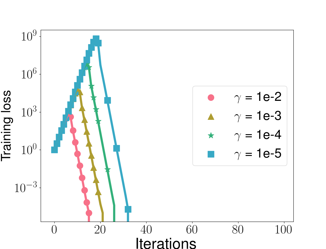
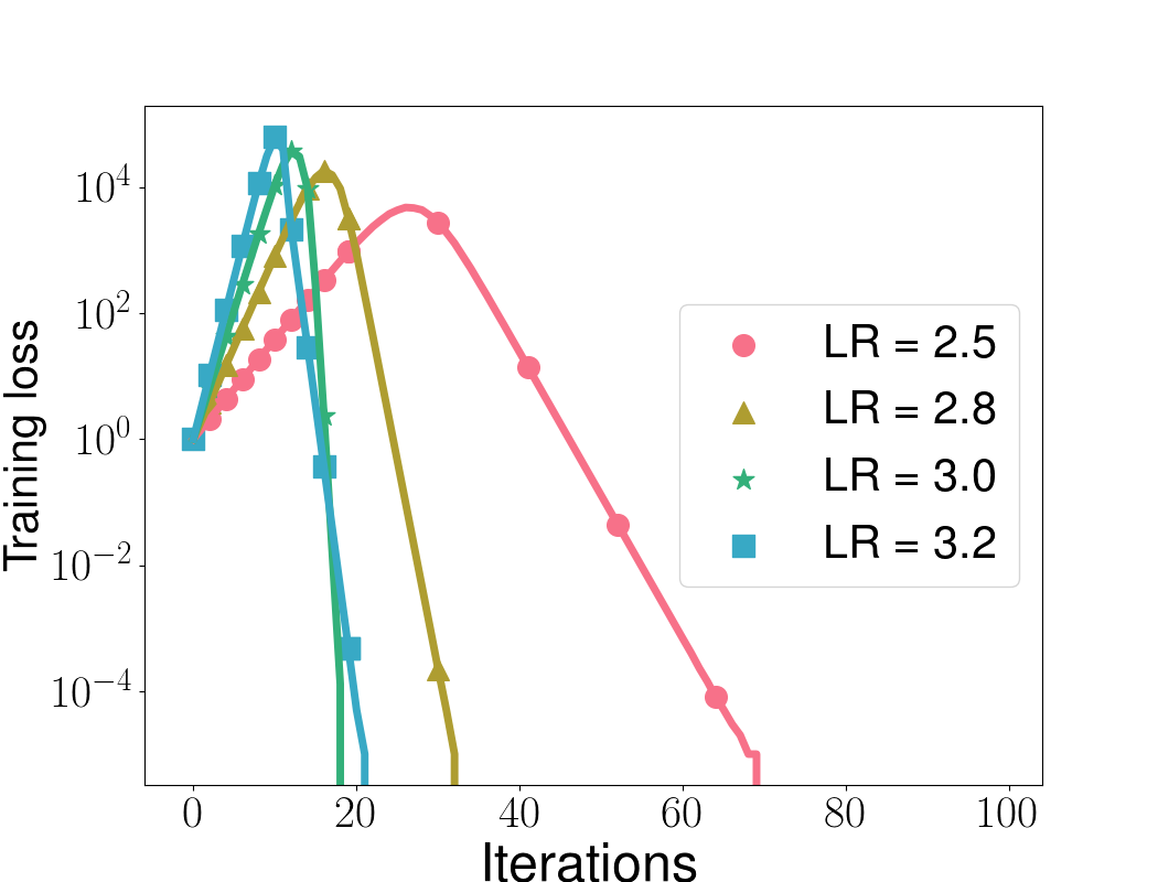
Using the inequality from Eq. (4), we obtain fquadflin=O~(1/m)normsubscript𝑓quadsubscript𝑓lin~𝑂1𝑚\|f_{{\mathrm{quad}}}-f_{{{\mathrm{lin}}}}\|=\tilde{O}(1/\sqrt{m}), hence fquadsubscript𝑓quadf_{{\mathrm{quad}}} transitions to linearity continuously as well in B(𝐰0,R)𝐵subscript𝐰0𝑅B({\mathbf{w}}_{0},R)333For general quadratic models in Eq. (3), the transition to linearity is continuously controlled by γ𝛾\gamma.. Given the continuous nature of the transition to linearity, one may expect that the transition from non-linear dynamics to linear dynamics for f𝑓f and fquadsubscript𝑓quadf_{{\mathrm{quad}}} is continuous in m𝑚m as well. Namely, one would expect that the domain of catapult dynamics, [ηcrit,ηmax]subscript𝜂critsubscript𝜂max[{\eta_{\mathrm{crit}}},{\eta_{\mathrm{max}}}], shrinks and ultimately converges to a single point, i.e., ηcrit=ηmaxsubscript𝜂critsubscript𝜂max{\eta_{\mathrm{crit}}}={\eta_{\mathrm{max}}}, as m𝑚m goes to infinity, with non-linear dynamics turning into linear dynamics. However, as shown both analytically and empirically, the transition is not continuous, for both network functions f𝑓f and NQMs fquadsubscript𝑓quadf_{{\mathrm{quad}}}, since the domain of the catapult dynamics can be independent of the width m𝑚m (or γ𝛾\gamma). Additionally, the length of the optimization path of f𝑓f in catapult dynamics grows with m𝑚m since otherwise, the optimization path could be contained in a ball with a constant radius independent of m𝑚m, in which f𝑓f can be approximated by flinsubscript𝑓linf_{{{\mathrm{lin}}}}. Since the optimization of flinsubscript𝑓linf_{{{\mathrm{lin}}}} diverges in catapult dynamics, by the approximation, the optimization of f𝑓f diverges as well, which contradicts the fact that the optimization of f𝑓f can converge in catapult dynamics (See Figure 2a).

2 Notation and preliminary

We use bold lowercase letters to denote vectors and capital letters to denote matrices. We denote the set {1,2,,n}12𝑛\{1,2,\cdots,n\} by [n]delimited-[]𝑛[n]. We use \|\cdot\| to denote the Euclidean norm for vectors and the spectral norm for matrices. We use direct-product\odot to denote element-wise multiplication (Hadamard product) for vectors. We use λmax(A)subscript𝜆𝐴\lambda_{\max}(A) and λmin(A)subscript𝜆𝐴\lambda_{\min}(A) to denote the largest and smallest eigenvalue of a matrix A𝐴A, respectively.

Given a model f(𝐰;𝒙)𝑓𝐰𝒙f({\mathbf{w}};{\boldsymbol{x}}), where 𝒙𝒙{\boldsymbol{x}} is input data and 𝐰𝐰{\mathbf{w}} are model parameters, we use 𝐰fsubscript𝐰𝑓\nabla_{\mathbf{w}}f to represent the partial first derivative f(𝐰;𝒙)/𝐰𝑓𝐰𝒙𝐰\partial f({\mathbf{w}};{\boldsymbol{x}})/\partial{\mathbf{w}}. When clear from context, we let f:=𝐰fassign𝑓subscript𝐰𝑓\nabla f:=\nabla_{{\mathbf{w}}}f for ease of notation. We use Hfsubscript𝐻𝑓H_{f} and Hsubscript𝐻H_{{\mathcal{L}}} to denote the Hessian (second derivative matrix) of the function f(𝐰;𝒙)𝑓𝐰𝒙f({\mathbf{w}};{\boldsymbol{x}}) and the loss (𝐰)𝐰{\mathcal{L}}({\mathbf{w}}) with respect to parameters 𝐰𝐰{\mathbf{w}}, respectively.

In the paper, we consider the following supervised learning task: given training data {(𝒙i,yi)}i=1nsuperscriptsubscriptsubscript𝒙𝑖subscript𝑦𝑖𝑖1𝑛\{({\boldsymbol{x}}_{i},y_{i})\}_{i=1}^{n} with data 𝒙idsubscript𝒙𝑖superscript𝑑{\boldsymbol{x}}_{i}\in\mathbb{R}^{d} and labels yisubscript𝑦𝑖y_{i}\in\mathbb{R} for i[n]𝑖delimited-[]𝑛i\in[n], we minimize the empirical risk with the squared loss (𝐰)=12i=1n(f(𝐰;𝒙i)yi)2𝐰12superscriptsubscript𝑖1𝑛superscript𝑓𝐰subscript𝒙𝑖subscript𝑦𝑖2{\mathcal{L}}({\mathbf{w}})=\frac{1}{2}\sum_{i=1}^{n}(f({\mathbf{w}};{\boldsymbol{x}}_{i})-y_{i})^{2}. Here f(𝐰;)𝑓𝐰f({\mathbf{w}};\cdot) is a parametric family of models, e.g., a neural network or a kernel machine, with parameters 𝐰p𝐰superscript𝑝{\mathbf{w}}\in\mathbb{R}^{p}. We use full-batch gradient descent to minimize the loss, and we denote trainable parameters 𝐰𝐰{\mathbf{w}} at iteration t𝑡t by 𝐰(t)𝐰𝑡{\mathbf{w}}(t). With constant step size (learning rate) η𝜂\eta, the update rule for the parameters is:

𝐰(t+1)=𝐰(t)ηd(𝐰)d𝐰(t),t0.formulae-sequence𝐰𝑡1𝐰𝑡𝜂𝑑𝐰𝑑𝐰𝑡for-all𝑡0\displaystyle\vspace{-5pt}{\mathbf{w}}(t+1)={\mathbf{w}}(t)-\eta\frac{d{\mathcal{L}}({\mathbf{w}})}{d{\mathbf{w}}}(t),~{}~{}\forall t\geq 0.
Definition 1 (Tangent Kernel).

The tangent kernel K(𝐰;,)𝐾𝐰K({\mathbf{w}};\cdot,\cdot) of f(𝐰;)𝑓𝐰f({\mathbf{w}};\cdot) is defined as

K(𝐰;𝒙,𝒛)=f(𝐰;𝒙),f(𝐰;𝒛),𝒙,𝒛d.formulae-sequence𝐾𝐰𝒙𝒛𝑓𝐰𝒙𝑓𝐰𝒛for-all𝒙𝒛superscript𝑑\displaystyle K({\mathbf{w}};{\boldsymbol{x}},{\boldsymbol{z}})=\langle\nabla f({\mathbf{w}};{\boldsymbol{x}}),\nabla f({\mathbf{w}};{\boldsymbol{z}})\rangle,~{}~{}~{}~{}\forall{\boldsymbol{x}},{\boldsymbol{z}}\in\mathbb{R}^{d}.\vspace{-5pt} (5)

In the context of the optimization problem with n𝑛n training examples, the tangent kernel matrix Kn×n𝐾superscript𝑛𝑛K\in\mathbb{R}^{n\times n} satisfies Ki,j(𝐰)=K(𝐰;𝒙i,𝒙j)subscript𝐾𝑖𝑗𝐰𝐾𝐰subscript𝒙𝑖subscript𝒙𝑗K_{i,j}({\mathbf{w}})=K({\mathbf{w}};{\boldsymbol{x}}_{i},{\boldsymbol{x}}_{j}), i,j[n]𝑖𝑗delimited-[]𝑛i,j\in[n]. The critical learning rate for optimization is given as follows.

Definition 2 (Critical learning rate).

With an initialization of parameters 𝐰0subscript𝐰0{\mathbf{w}}_{0}, the critical learning rate of f(𝐰;)𝑓𝐰f({\mathbf{w}};\cdot) is defined as

ηcrit:=2/λmax(H(𝐰0)).assignsubscript𝜂crit2subscript𝜆subscript𝐻subscript𝐰0\displaystyle\vspace{-10pt}{\eta_{\mathrm{crit}}}:=2/\lambda_{\max}(H_{{\mathcal{L}}}({\mathbf{w}}_{0})). (6)

A learning rate η𝜂\eta is said to be sub-critical if 0<η<ηcrit0𝜂subscript𝜂crit0<\eta<{\eta_{\mathrm{crit}}} or super-critical if ηcrit<η<ηmaxsubscript𝜂crit𝜂subscript𝜂{\eta_{\mathrm{crit}}}<\eta<\eta_{\max}. Here ηmaxsubscript𝜂max{\eta_{\mathrm{max}}} is the maximum leaning rate such that the optimization of (𝐰)𝐰{\mathcal{L}}({\mathbf{w}}) initialized at 𝐰0subscript𝐰0{\mathbf{w}}_{0} can converge.

Dynamics for Linear models.

When f𝑓f is linear in 𝐰𝐰{\mathbf{w}}, the gradient, f𝑓\nabla f, and tangent kernel are constant: K(𝐰(t))=K(𝐰0)𝐾𝐰𝑡𝐾subscript𝐰0K({\mathbf{w}}(t))=K({\mathbf{w}}_{0}). Therefore, gradient descent dynamics are:

F(𝐰(t+1))𝐲𝐹𝐰𝑡1𝐲\displaystyle F({\mathbf{w}}(t+1))-{\mathbf{y}} =(IηK(𝐰0))(F(𝐰(t))𝐲),t0,formulae-sequenceabsent𝐼𝜂𝐾subscript𝐰0𝐹𝐰𝑡𝐲for-all𝑡0\displaystyle=(I-\eta K({\mathbf{w}}_{0}))(F({\mathbf{w}}(t))-{\mathbf{y}}),~{}~{}~{}\forall t\geq 0, (7)

where F(𝐰0)=[f1(𝐰0),,fn(𝐰0)]T𝐹subscript𝐰0superscriptsubscript𝑓1subscript𝐰0subscript𝑓𝑛subscript𝐰0𝑇F({\mathbf{w}}_{0})=[f_{1}({\mathbf{w}}_{0}),...,f_{n}({\mathbf{w}}_{0})]^{T} with fi(𝐰0)=f(𝐰0;𝒙i)subscript𝑓𝑖subscript𝐰0𝑓subscript𝐰0subscript𝒙𝑖f_{i}({\mathbf{w}}_{0})=f({\mathbf{w}}_{0};{\boldsymbol{x}}_{i}).

Noting that H(𝐰0)=F(𝐰0)TF(𝐰0)subscript𝐻subscript𝐰0𝐹superscriptsubscript𝐰0𝑇𝐹subscript𝐰0H_{{\mathcal{L}}}({\mathbf{w}}_{0})=\nabla F({\mathbf{w}}_{0})^{T}\nabla F({\mathbf{w}}_{0}) and that tangent kernel K(𝐰0)=F(𝐰0)F(𝐰0)T𝐾subscript𝐰0𝐹subscript𝐰0𝐹superscriptsubscript𝐰0𝑇K({\mathbf{w}}_{0})=\nabla F({\mathbf{w}}_{0})\nabla F({\mathbf{w}}_{0})^{T} share the same positive eigenvalues, we have λmax(H(𝐰0))=λmax(K(𝐰0))subscript𝜆subscript𝐻subscript𝐰0subscript𝜆𝐾subscript𝐰0\lambda_{\max}(H_{{\mathcal{L}}}({\mathbf{w}}_{0}))=\lambda_{\max}(K({\mathbf{w}}_{0})), and hence,

ηcrit=2/λmax(K(𝐰0)).subscript𝜂crit2subscript𝜆𝐾subscript𝐰0{\eta_{\mathrm{crit}}}=2/\lambda_{\max}(K({\mathbf{w}}_{0})). (8)

Therefore, from Eq. (7), if 0<η<ηcrit0𝜂subscript𝜂crit0<\eta<{\eta_{\mathrm{crit}}}, the loss {\mathcal{L}} decreases monotonically and if η>ηcrit𝜂subscript𝜂crit\eta>{\eta_{\mathrm{crit}}}, the loss {\mathcal{L}} keeps increasing. Note that the critical and maximum learning rates are equal in this setting.

3 Optimization dynamics in Neural Quadratic Models

In this section, we analyze the gradient descent dynamics of the NQM corresponding to a two-layer fully-connected neural network. We show that, unlike a linear model, the NQM exhibits a catapult dynamics: the loss increases at the early stage of training then decreases afterwards. We further show that the top eigenvalues of the tangent kernel typically become smaller as a consequence of the catapult.

Neural Quadratic Model (NQM).

Consider the NQM that approximates the following two-layer neural network:

f(𝐮,𝐯;𝒙)=1mi=1mviσ(1d𝐮iT𝒙),𝑓𝐮𝐯𝒙1𝑚superscriptsubscript𝑖1𝑚subscript𝑣𝑖𝜎1𝑑superscriptsubscript𝐮𝑖𝑇𝒙\displaystyle f({\mathbf{u}},{\mathbf{v}};{\boldsymbol{x}})=\frac{1}{\sqrt{m}}\sum_{i=1}^{m}v_{i}\sigma\left(\frac{1}{\sqrt{d}}{\mathbf{u}}_{i}^{T}{\boldsymbol{x}}\right), (9)

where 𝐮idsubscript𝐮𝑖superscript𝑑{\mathbf{u}}_{i}\in\mathbb{R}^{d}, visubscript𝑣𝑖v_{i}\in\mathbb{R} for i[m]𝑖delimited-[]𝑚i\in[m] are trainable parameters, 𝒙d𝒙superscript𝑑{\boldsymbol{x}}\in\mathbb{R}^{d} is the input, and σ()𝜎\sigma(\cdot) is the ReLU activation function. We initialize 𝐮i𝒩(0,Id)similar-tosubscript𝐮𝑖𝒩0subscript𝐼𝑑{\mathbf{u}}_{i}\sim\mathcal{N}(0,I_{d}) and viUnif[{1,1}]subscript𝑣𝑖Unifdelimited-[]11v_{i}\in\mathrm{Unif}[\{-1,1\}] for each i𝑖i independently. Letting g(𝐮,𝐯;𝒙):=fquad(𝐮,𝐯;𝒙)assign𝑔𝐮𝐯𝒙subscript𝑓quad𝐮𝐯𝒙g({\mathbf{u}},{\mathbf{v}};{\boldsymbol{x}}):=f_{\mathrm{quad}}({\mathbf{u}},{\mathbf{v}};{\boldsymbol{x}}), this NQM has the following expression (See the full derivation in Appendix A):

g(𝐮,𝐯;𝒙)𝑔𝐮𝐯𝒙\displaystyle g({\mathbf{u}},{\mathbf{v}};{\boldsymbol{x}}) =f(𝐮0,𝐯0;𝒙)+1mdi=1mv0,i(𝐮i𝐮0,i)T𝒙𝟙{𝐮0,iT𝒙0}+1mdi=1m(viv0,i)σ(𝐮0,iT𝒙)absent𝑓subscript𝐮0subscript𝐯0𝒙1𝑚𝑑superscriptsubscript𝑖1𝑚subscript𝑣0𝑖superscriptsubscript𝐮𝑖subscript𝐮0𝑖𝑇𝒙subscript1superscriptsubscript𝐮0𝑖𝑇𝒙01𝑚𝑑superscriptsubscript𝑖1𝑚subscript𝑣𝑖subscript𝑣0𝑖𝜎superscriptsubscript𝐮0𝑖𝑇𝒙\displaystyle=f({\mathbf{u}}_{0},{\mathbf{v}}_{0};{\boldsymbol{x}})+\frac{1}{\sqrt{md}}\sum_{i=1}^{m}v_{0,i}({\mathbf{u}}_{i}-{\mathbf{u}}_{0,i})^{T}{\boldsymbol{x}}\mathbbm{1}_{\left\{{\mathbf{u}}_{0,i}^{T}{\boldsymbol{x}}\geq 0\right\}}+\frac{1}{\sqrt{md}}\sum_{i=1}^{m}(v_{i}-v_{0,i})\sigma\left({\mathbf{u}}_{0,i}^{T}{\boldsymbol{x}}\right)
+1mdi=1m(viv0,i)(𝐮i𝐮0,i)T𝒙𝟙{𝐮0,iT𝒙0}.1𝑚𝑑superscriptsubscript𝑖1𝑚subscript𝑣𝑖subscript𝑣0𝑖superscriptsubscript𝐮𝑖subscript𝐮0𝑖𝑇𝒙subscript1superscriptsubscript𝐮0𝑖𝑇𝒙0\displaystyle~{}~{}~{}~{}+\frac{1}{\sqrt{md}}\sum_{i=1}^{m}(v_{i}-v_{0,i})({\mathbf{u}}_{i}-{\mathbf{u}}_{0,i})^{T}{\boldsymbol{x}}\mathbbm{1}_{\left\{{\mathbf{u}}_{0,i}^{T}{\boldsymbol{x}}\geq 0\right\}}. (10)

Given training data {𝒙i,yi}i=1nsuperscriptsubscriptsubscript𝒙𝑖subscript𝑦𝑖𝑖1𝑛\{{\boldsymbol{x}}_{i},y_{i}\}_{i=1}^{n}, we minimize the empirical risk with the squared loss (𝐰)=12i=1n(g(𝐰;𝒙i)yi)2𝐰12superscriptsubscript𝑖1𝑛superscript𝑔𝐰subscript𝒙𝑖subscript𝑦𝑖2{\mathcal{L}}({\mathbf{w}})=\frac{1}{2}\sum_{i=1}^{n}(g({\mathbf{w}};{\boldsymbol{x}}_{i})-y_{i})^{2} using GD with constant learning rate η𝜂\eta. Throughout this section, we denote g(𝐮(t),𝐯(t);𝒙)𝑔𝐮𝑡𝐯𝑡𝒙g({\mathbf{u}}(t),{\mathbf{v}}(t);{\boldsymbol{x}}) by g(t)𝑔𝑡g(t) and its tangent kernel K(𝐮(t),𝐯(t))𝐾𝐮𝑡𝐯𝑡K({\mathbf{u}}(t),{\mathbf{v}}(t)) by K(t)𝐾𝑡K(t), where t𝑡t is the iteration of GD. We assume 𝒙i=O(1)normsubscript𝒙𝑖𝑂1\|{\boldsymbol{x}}_{i}\|=O(1) and |yi|=O(1)subscript𝑦𝑖𝑂1|y_{i}|=O(1) for i[n]𝑖delimited-[]𝑛i\in[n], and we assume the width of f𝑓f is much larger than the input dimension d𝑑d and the data size n𝑛n, i.e., mmax{d,n}much-greater-than𝑚𝑑𝑛m\gg\max\{d,n\}. Hence, d𝑑d and n𝑛n can be regarded as small constants. In the whole paper, we use the big-O and small-o notation with respect to the width m𝑚m. Below, we start with the single training example case, which already showcases the non-linear dynamics of NQMs.

3.1 Catapult dynamics with a single training example

In this subsection, we consider training dynamics of NQM Eq. (3) with a single training example (𝒙,y)𝒙𝑦({\boldsymbol{x}},y) where 𝒙d𝒙superscript𝑑{\boldsymbol{x}}\in\mathbb{R}^{d} and y𝑦y\in\mathbb{R}. In this case, the tangent kernel matrix K𝐾K reduces to a scalar, and we denote K𝐾K by λ𝜆\lambda to distinguish it from a matrix.

By gradient descent with step size η𝜂\eta, the updates for g(t)y𝑔𝑡𝑦g(t)-y and λ(t)𝜆𝑡\lambda(t), which we refer to as dynamics equations, can be derived as follows (see the derivation in Appendix B.1):

Dynamics equations.

g(t+1)y𝑔𝑡1𝑦\displaystyle g(t+1)-y =(1ηλ(t)+𝒙2mdη2(g(t)y)g(t)Rg(t))(g(t)y):=μ(t)(g(t)y),absent1𝜂𝜆𝑡subscriptsuperscriptnorm𝒙2𝑚𝑑superscript𝜂2𝑔𝑡𝑦𝑔𝑡subscript𝑅𝑔𝑡𝑔𝑡𝑦assign𝜇𝑡𝑔𝑡𝑦\displaystyle=\left(1-\eta\lambda(t)+\underbrace{\frac{\|{\boldsymbol{x}}\|^{2}}{md}\eta^{2}(g(t)-y)g(t)}_{R_{g}(t)}\right)(g(t)-y):=\mu(t)(g(t)-y), (11)
λ(t+1)𝜆𝑡1\displaystyle\lambda(t+1) =λ(t)η𝒙2md(g(t)y)2(4g(t)g(t)yηλ(t))Rλ(t),t0.formulae-sequenceabsent𝜆𝑡subscript𝜂superscriptnorm𝒙2𝑚𝑑superscript𝑔𝑡𝑦24𝑔𝑡𝑔𝑡𝑦𝜂𝜆𝑡subscript𝑅𝜆𝑡for-all𝑡0\displaystyle=\lambda(t)-\underbrace{\eta\frac{\|{\boldsymbol{x}}\|^{2}}{md}(g(t)-y)^{2}\left(4\frac{g(t)}{g(t)-y}-\eta\lambda(t)\right)}_{R_{\lambda}(t)},~{}~{}~{}~{}\forall t\geq 0.\vspace{-5pt} (12)

Note that as the loss is given by (t)=12(g(t)y)2𝑡12superscript𝑔𝑡𝑦2{\mathcal{L}}(t)=\frac{1}{2}(g(t)-y)^{2}, to understand convergence, it suffices to analyze the dynamics equations above. Compared to the linear dynamics Eq. (7), this non-linear dynamics has extra terms Rg(t)subscript𝑅𝑔𝑡R_{g}(t) and Rλ(t)subscript𝑅𝜆𝑡R_{\lambda}(t), which are induced by the non-linear term in the NQM. We will see that the convergence of gradient descent depends on the scale and sign of Rg(t)subscript𝑅𝑔𝑡R_{g}(t) and Rλ(t)subscript𝑅𝜆𝑡R_{\lambda}(t). For example, for constant learning rate that is slightly larger than ηcritsubscript𝜂crit{\eta_{\mathrm{crit}}} (which would result in divergence for linear models), Rλ(t)subscript𝑅𝜆𝑡R_{\lambda}(t) stays positive during training, resulting in both monotonic decrease of tangent kernel λ𝜆\lambda and the loss.

As λ(t)=λ0+τ=0tRλ(τ)𝜆𝑡subscript𝜆0superscriptsubscript𝜏0𝑡subscript𝑅𝜆𝜏\lambda(t)=\lambda_{0}+\sum_{\tau=0}^{t}R_{\lambda}(\tau), to track the scale of |μ(t)|𝜇𝑡|\mu(t)|, we will focus on the scale and sign of Rg(t)subscript𝑅𝑔𝑡R_{g}(t) and Rλ(t)subscript𝑅𝜆𝑡R_{\lambda}(t) in the following analysis. For the scale of λ0subscript𝜆0\lambda_{0}, which is non-negative by Definition 1, we can show that with high probability over random initialization, |λ0|=Θ(1)subscript𝜆0Θ1|\lambda_{0}|=\Theta(1) (see Appendix I). And |g(0)|=O(1)𝑔0𝑂1|g(0)|=O(1) with high probability as well [5]. Therefore the following discussion is with high probability over random initialization. We start by establishing monotonic convergence for sub-critical learning rates.

Monotonic convergence: sub-critical learning rates (η<2/λ0=ηcrit𝜂2subscript𝜆0subscript𝜂crit\eta<2/\lambda_{0}={\eta_{\mathrm{crit}}}).

The key observation is that when |g(t)|=O(1)𝑔𝑡𝑂1|g(t)|=O(1), and λ(t)=Θ(1)𝜆𝑡Θ1\lambda(t)=\Theta(1), |Rg(t)|subscript𝑅𝑔𝑡|R_{g}(t)| and |Rλ(t)|subscript𝑅𝜆𝑡|R_{\lambda}(t)| are of the order o(1)𝑜1o(1). Then, the dynamics equations approximately reduce to the ones of linear dynamics:

g(t+1)y𝑔𝑡1𝑦\displaystyle g(t+1)-y =(1ηλ(t)+o(1))(g(t)y),absent1𝜂𝜆𝑡𝑜1𝑔𝑡𝑦\displaystyle=\left(1-\eta\lambda(t)+o(1)\right)(g(t)-y),
λ(t+1)𝜆𝑡1\displaystyle\lambda(t+1) =λ(t)+o(1).absent𝜆𝑡𝑜1\displaystyle=\lambda(t)+o(1).

Note that at initialization, the output satisfies |g(0)|=O(1)𝑔0𝑂1|g(0)|=O(1), and we have shown λ0=Θ(1)subscript𝜆0Θ1\lambda_{0}=\Theta(1). With the choice of η𝜂\eta, we have for all t0𝑡0t\geq 0, |μ(t)|=|1ηλ(t)+o(1)|<1𝜇𝑡1𝜂𝜆𝑡𝑜11|\mu(t)|=|1-\eta\lambda(t)+o(1)|<1; hence, |g(t)y|𝑔𝑡𝑦|g(t)-y| decreases monotonically. The cumulative change on the tangent kernel will be o(1)𝑜1o(1), i.e., t|Rλ(t)|=o(1)subscript𝑡subscript𝑅𝜆𝑡𝑜1\sum_{t}|R_{\lambda}(t)|=o(1), since for all t𝑡t, |Rλ(t)|=O(1/m)subscript𝑅𝜆𝑡𝑂1𝑚|R_{\lambda}(t)|=O(1/m) and the loss decreases exponentially hence |Rλ(t)|=O(1/m)logO(1)=o(1)subscript𝑅𝜆𝑡𝑂1𝑚𝑂1𝑜1\sum|R_{\lambda}(t)|=O(1/m)\cdot\log O(1)=o(1). See Appendix C for a detailed discussion.

Catapult convergence: super-critical learning rates (ηcrit=2/λ0<η<4/λ0=ηmaxsubscript𝜂crit2subscript𝜆0𝜂4subscript𝜆0subscript𝜂max{\eta_{\mathrm{crit}}}=2/\lambda_{0}<\eta<4/\lambda_{0}={\eta_{\mathrm{max}}}).

The training dynamics are given by the following theorem.

Theorem 1 (Catapult dynamics on a single training example).

Consider training the NQM Eq. (3) with squared loss on a single training example by GD. With a super-critical learning rate η[2+ϵλ0,4ϵλ0]𝜂2italic-ϵsubscript𝜆04italic-ϵsubscript𝜆0\eta\in\left[\frac{2+\epsilon}{\lambda_{0}},\frac{4-\epsilon}{\lambda_{0}}\right] where ϵ=Θ(logmm)italic-ϵΘ𝑚𝑚\epsilon=\Theta\left(\frac{\log m}{\sqrt{m}}\right), the catapult happens: the loss increases to the order of Ω(m(η2/λ0)2logm)Ω𝑚superscript𝜂2subscript𝜆02𝑚\Omega\left(\frac{m(\eta-2/\lambda_{0})^{2}}{\log m}\right) then decreases to O(1)𝑂1O(1).

Proof of Theorem 1.

We use the following transformation of the variables to simplify notations.

u(t)=𝒙2mdη2(g(t)y)2,w(t)=𝒙2mdη2(g(t)y)y,v(t)=ηλ(t).formulae-sequence𝑢𝑡superscriptnorm𝒙2𝑚𝑑superscript𝜂2superscript𝑔𝑡𝑦2formulae-sequence𝑤𝑡superscriptnorm𝒙2𝑚𝑑superscript𝜂2𝑔𝑡𝑦𝑦𝑣𝑡𝜂𝜆𝑡\displaystyle u(t)=\frac{\norm{{\boldsymbol{x}}}^{2}}{md}\eta^{2}(g(t)-y)^{2},~{}~{}~{}w(t)=\frac{\|{\boldsymbol{x}}\|^{2}}{md}\eta^{2}(g(t)-y)y,~{}~{}~{}v(t)=\eta\lambda(t).

Then the Eq. (11) and Eq. (12) are reduced to

u(t+1)𝑢𝑡1\displaystyle u(t+1) =(1v(t)+u(t)+w(t))2u(t):=κ(t)u(t),absentsuperscript1𝑣𝑡𝑢𝑡𝑤𝑡2𝑢𝑡assign𝜅𝑡𝑢𝑡\displaystyle=(1-v(t)+u(t)+w(t))^{2}u(t):=\kappa(t)u(t), (13)
v(t+1)𝑣𝑡1\displaystyle v(t+1) =v(t)u(t)(4v(t))4w(t).absent𝑣𝑡𝑢𝑡4𝑣𝑡4𝑤𝑡\displaystyle=v(t)-u(t)(4-v(t))-4w(t). (14)

At initialization, since |g(0)|=O(1)𝑔0𝑂1|g(0)|=O(1), we have u(0)=O(1m)𝑢0𝑂1𝑚u(0)=O\left(\frac{1}{m}\right) and w(0)=O(1m)𝑤0𝑂1𝑚w(0)=O\left(\frac{1}{m}\right). Note that by definition, for all t0𝑡0t\geq 0, u(t)0𝑢𝑡0u(t)\geq 0 and we have v(t)0𝑣𝑡0v(t)\geq 0 since λ(t)𝜆𝑡\lambda(t) is the tangent kernel for a single training example.

In the following, we will analyze the above dynamical equations. To make the analysis more understandable, we separate the dynamics during training into increasing phase and decreasing phase. We denote δ:=ηηcrit=η2/λ0assign𝛿𝜂subscript𝜂crit𝜂2subscript𝜆0\delta:=\eta-{\eta_{\mathrm{crit}}}=\eta-2/\lambda_{0}.

Increasing phase.

In this phase, |u(t)|𝑢𝑡|u(t)| increases exponentially from O(1m)𝑂1𝑚O\left(\frac{1}{m}\right) to Θ(δ2logm)Θsuperscript𝛿2𝑚\Theta\left(\frac{\delta^{2}}{\log m}\right) and |v(t)v(0)|=O(δ2logm)𝑣𝑡𝑣0𝑂superscript𝛿2𝑚|v(t)-v(0)|=O\left(\frac{\delta^{2}}{\log m}\right). This can be shown by the following lemma.

Lemma 1.

For T>0𝑇0T>0 such that supt[0,T]u(t)=O(δ2logm)subscriptsupremum𝑡0𝑇𝑢𝑡𝑂superscript𝛿2𝑚\sup_{t\in[0,T]}u(t)=O\left(\frac{\delta^{2}}{\log m}\right), u(t)𝑢𝑡u(t) increases exponentially with inft[0,T]κ(t)=(1+δO(δ2logm))2>1subscriptinfimum𝑡0𝑇𝜅𝑡superscript1𝛿𝑂superscript𝛿2𝑚21\inf_{t\in[0,T]}\kappa(t)=\left(1+\delta-O\left(\frac{\delta^{2}}{\log m}\right)\right)^{2}>1 and supt[0,T]|v(t)v(0)|=O(δ2logm)subscriptsupremum𝑡0𝑇𝑣𝑡𝑣0𝑂superscript𝛿2𝑚\sup_{t\in[0,T]}|v(t)-v(0)|=O\left(\frac{\delta^{2}}{\log m}\right).

Proof.

See the proof in Section D. ∎

After the increasing phase, based on the order of u(t)𝑢𝑡u(t) we can infer the order of loss is Θ(mδ2logm)Θ𝑚superscript𝛿2𝑚\Theta\left(\frac{m\delta^{2}}{\log m}\right).

Decreasing phase.

When u(t)𝑢𝑡u(t) is sufficiently large, v(t)𝑣𝑡v(t) will have non-negligible decrease which leads to the decreasing of κ(t)𝜅𝑡\kappa(t), hence in turn making u(t)𝑢𝑡u(t) decrease as well. Consequently, we have:

Lemma 2.

There exists T>0superscript𝑇0T^{*}>0 such that u(T)=O(1m)𝑢superscript𝑇𝑂1𝑚u(T^{*})=O\left(\frac{1}{m}\right).

Proof.

See the proof in Section E. ∎

Then accordingly, the loss is of the order O(1)𝑂1O(1). ∎ Once the loss decreases to the order of O(1)𝑂1O(1), the catapult finishes and we in general have η<2/λ(t)𝜂2𝜆𝑡\eta<2/\lambda(t) as |μ(t)|=|1ηλ(t)+R𝐠(t)|<1𝜇𝑡1𝜂𝜆𝑡subscript𝑅𝐠𝑡1|\mu(t)|=|1-\eta\lambda(t)+R_{\mathbf{g}}(t)|<1 where |R𝐠(t)|=O((t)/m)=O(1/m)subscript𝑅𝐠𝑡𝑂𝑡𝑚𝑂1𝑚|R_{\mathbf{g}}(t)|=O({\mathcal{L}}(t)/m)=O(1/m). Therefore the training dynamics fall into linear dynamics, and we can use the same analysis for sub-critical learning rates for the remaining training dynamics. The stableness of the steady-state equilibria of dynamical equations can be guaranteed by the following:

Theorem 2.

For dynamical equations Eq. (11) and (12), the stable steady-state equilibria satisfy g(t)=y𝑔𝑡𝑦g(t)=y (i.e.,loss is 00), and λ(t)[ϵ,2/ηϵ]𝜆𝑡italic-ϵ2𝜂italic-ϵ\lambda(t)\in[\epsilon,2/\eta-\epsilon] with ϵ=Θ(logm/m)italic-ϵΘ𝑚𝑚\epsilon=\Theta(\log m/\sqrt{m}).

Divergence (η>ηmax=4/λ0𝜂subscript𝜂4subscript𝜆0\eta>\eta_{\max}=4/\lambda_{0}).

Initially, it follows the same dynamics with that in the increasing phase in catapult convergence: |g(t)y|𝑔𝑡𝑦|g(t)-y| increases exponentially as |μ(t)|>1𝜇𝑡1|\mu(t)|>1 and the λ(t)𝜆𝑡\lambda(t) almost does not change as Rλ(t)subscript𝑅𝜆𝑡R_{\lambda}(t) is small. However, note that Rλ(t)>0subscript𝑅𝜆𝑡0R_{\lambda}(t)>0 since 1) g(t)/(g(t)y)1𝑔𝑡𝑔𝑡𝑦1g(t)/(g(t)-y)\approx 1 when g(t)𝑔𝑡g(t) becomes large and 2) η>4/λ(t)𝜂4𝜆𝑡\eta>4/\lambda(t). Therefore, λ(t)𝜆𝑡\lambda(t) keeps increasing during training, which consequently leads to the divergence of the optimization. See Appendix G for a detailed discussion.

3.2 Catapult dynamics with multiple training examples

In this subsection we show the catapult phase will happen for NQMs Eq. (9) with multiple training examples. We assume unidimensional input data, which is common in the literature and simplifies the analysis for neural networks (see for example  [26, 25]).

Assumption 1.

The input dimension d=1𝑑1d=1 and not all xisubscript𝑥𝑖x_{i} is 00, i.e., |xi|>0subscript𝑥𝑖0\sum|x_{i}|>0.

We similarly analyze the dynamics equations with different learning rates for multiple training examples (see the derivation of Eq. (18) and (19) in Appendix) which are update equations of 𝐠(t)𝐲𝐠𝑡𝐲{\mathbf{g}}(t)-{\mathbf{y}} and K(t)𝐾𝑡K(t). And similarly, we show there are three training dynamics: monotonic convergence, catapult convergence and divergence.

In the analysis, we consider the training dynamics projected to two orthogonal eigenvectors of the tangent kernel, i.e., 𝒑1subscript𝒑1{\boldsymbol{p}}_{1} and 𝒑2subscript𝒑2{\boldsymbol{p}}_{2}, and we show with different learning rates, the catapult phase can occur only in the direction of 𝒑1subscript𝒑1{\boldsymbol{p}}_{1}, or occur in both directions. We consider the case where 2/λ2(0)<4/λ1(0)2subscript𝜆204subscript𝜆102/\lambda_{2}(0)<4/\lambda_{1}(0) hence the catapult can occur in both directions. The analysis for the other case can be directly obtained from our results. We denote the loss projected to 𝒑isubscript𝒑𝑖{\boldsymbol{p}}_{i} by Πi:=12𝐠𝐲,𝒑i2assignsubscriptΠ𝑖12superscript𝐠𝐲subscript𝒑𝑖2\Pi_{i}{\mathcal{L}}:=\frac{1}{2}\left<{\mathbf{g}}-{\mathbf{y}},{\boldsymbol{p}}_{i}\right>^{2} for i=1,2𝑖12i=1,2. We have Πi(0)=O(1)subscriptΠ𝑖0𝑂1\Pi_{i}{\mathcal{L}}(0)=O(1) with high probability over random initialization of weights.

We formulate the result for the catapult dynamics, which happens when training with super-critical learning rates, into the following theorem, and defer the proof of it and the full discussion of training dynamics to Appendix K.

Theorem 3 (Catapult dynamics on multiple training examples).

Supposing Assumption 1 holds, consider training the NQM Eq. (3) with squared loss on multiple training examples by GD. Then,

  1. 1.

    with η[2+ϵλ1(0),2ϵλ2(0)]𝜂2italic-ϵsubscript𝜆102italic-ϵsubscript𝜆20\eta\in\left[\frac{2+\epsilon}{\lambda_{1}(0)},\frac{2-\epsilon}{\lambda_{2}(0)}\right] , the catapult only occurs in eigendirection 𝒑1subscript𝒑1{\boldsymbol{p}}_{1}: Π1subscriptΠ1\Pi_{1}{\mathcal{L}} increases to the order of Ω(m(η2/λ1(0))2logm)Ω𝑚superscript𝜂2subscript𝜆102𝑚\Omega\left(\frac{m(\eta-2/\lambda_{1}(0))^{2}}{\log m}\right) then decreases to O(1)𝑂1O(1);

  2. 2.

    with η[2+ϵλ2(0),4ϵλ1(0)]𝜂2italic-ϵsubscript𝜆204italic-ϵsubscript𝜆10\eta\in\left[\frac{2+\epsilon}{\lambda_{2}(0)},\frac{4-\epsilon}{\lambda_{1}(0)}\right], the catapult occurs in both eigendirections 𝒑1subscript𝒑1{\boldsymbol{p}}_{1} and 𝒑2subscript𝒑2{\boldsymbol{p}}_{2}: ΠisubscriptΠ𝑖\Pi_{i}{\mathcal{L}} for i=1,2𝑖12i=1,2 increases to the order of Ω(m(η2/λi(0))2logm)Ω𝑚superscript𝜂2subscript𝜆𝑖02𝑚\Omega\left(\frac{m(\eta-2/\lambda_{i}(0))^{2}}{\log m}\right) then decreases to O(1)𝑂1O(1),

where ϵ=Θ(logmm)italic-ϵΘ𝑚𝑚\epsilon=\Theta\left(\frac{\log m}{\sqrt{m}}\right).

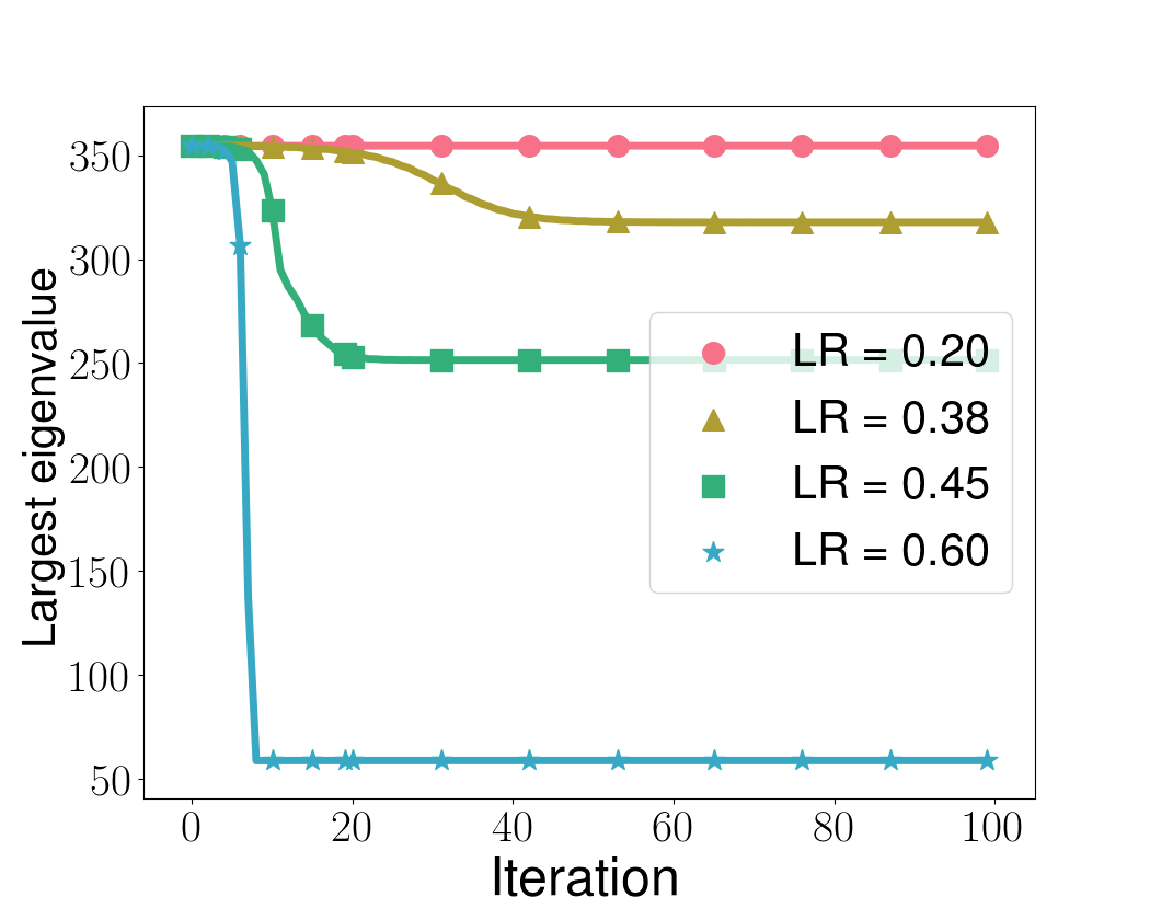
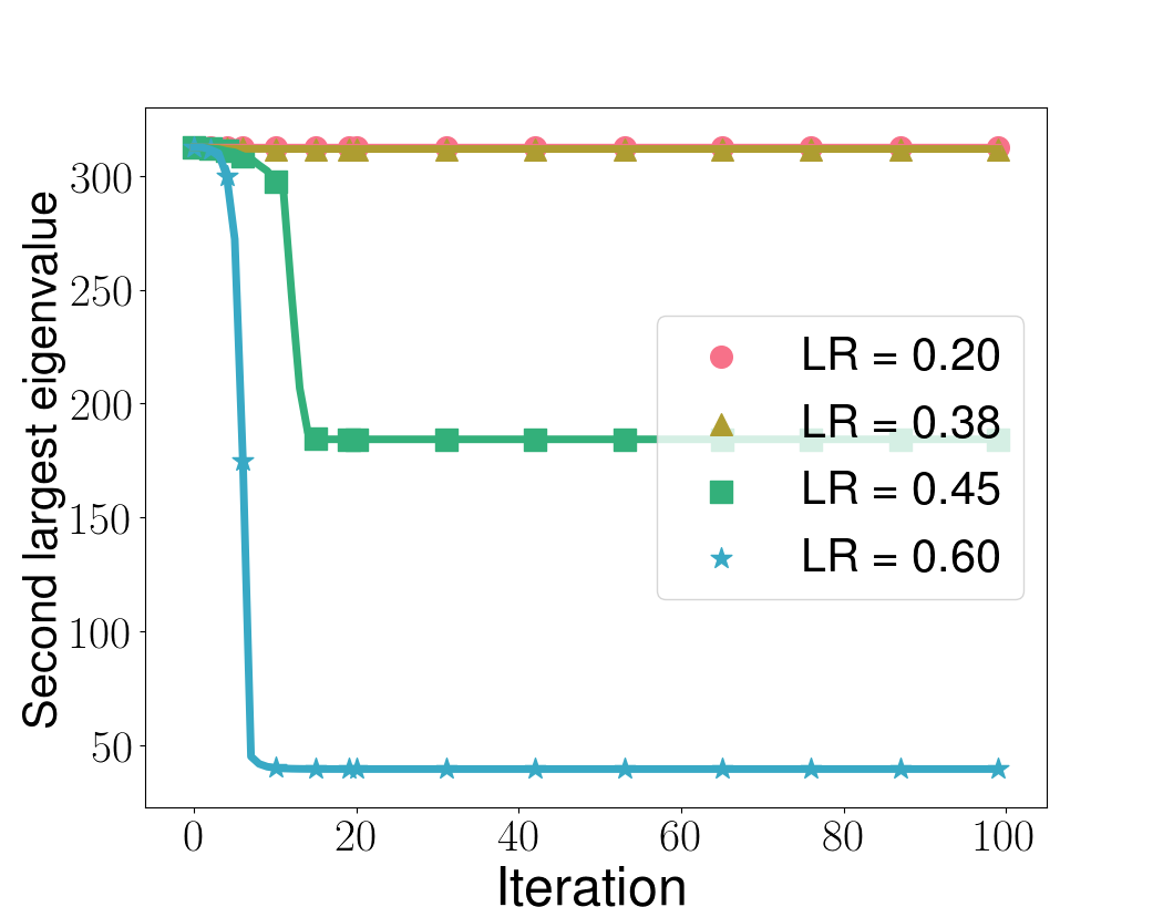
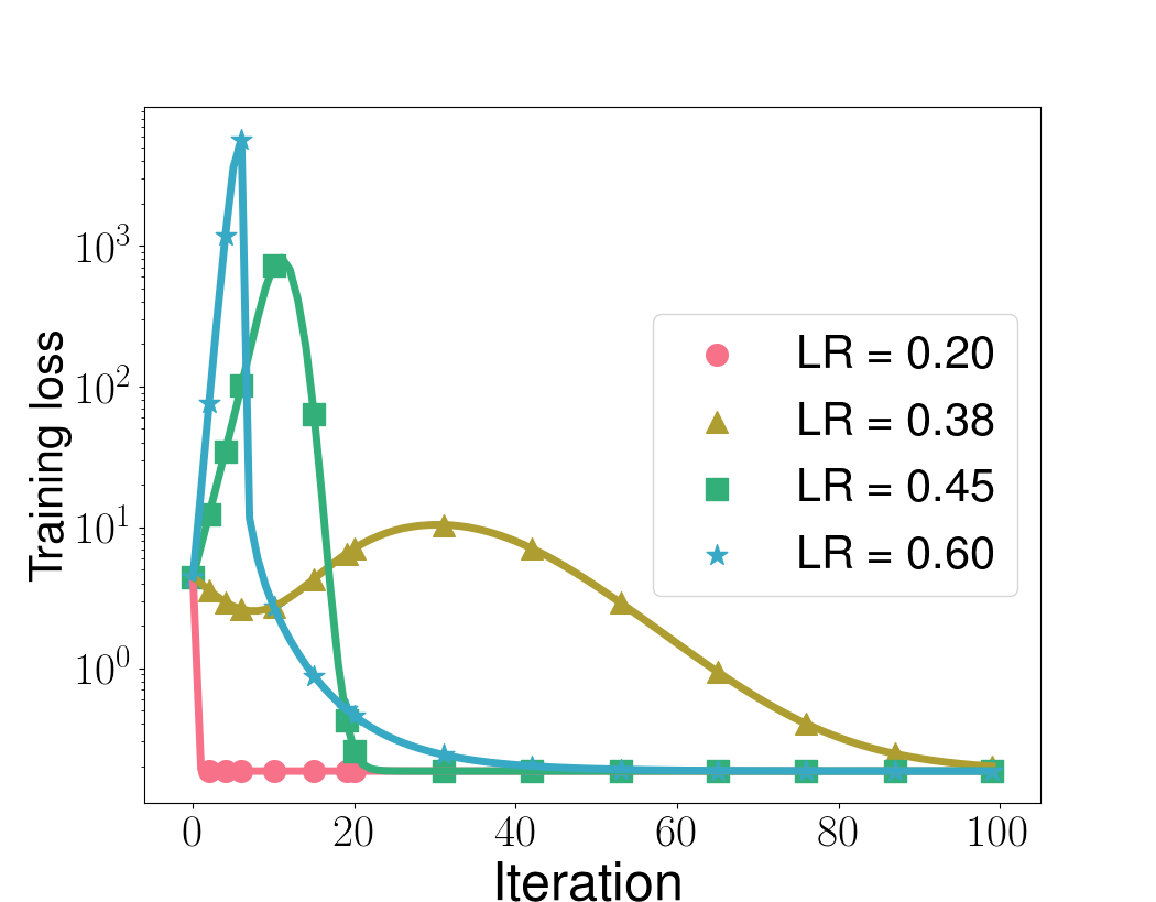
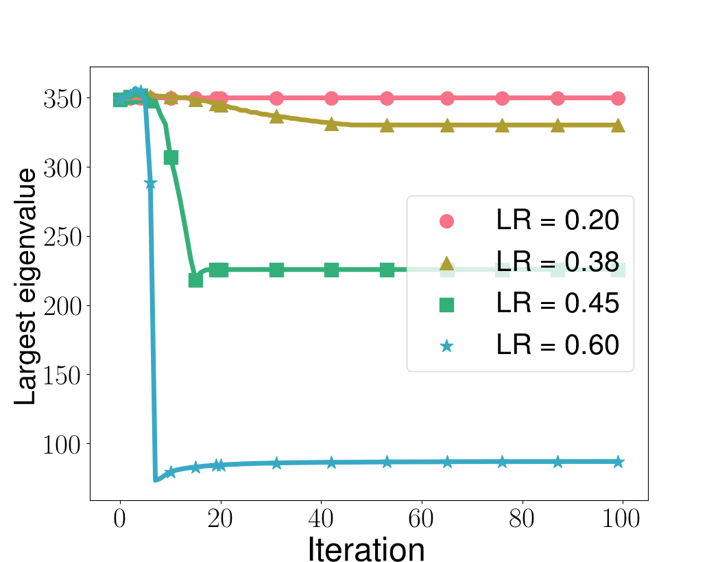
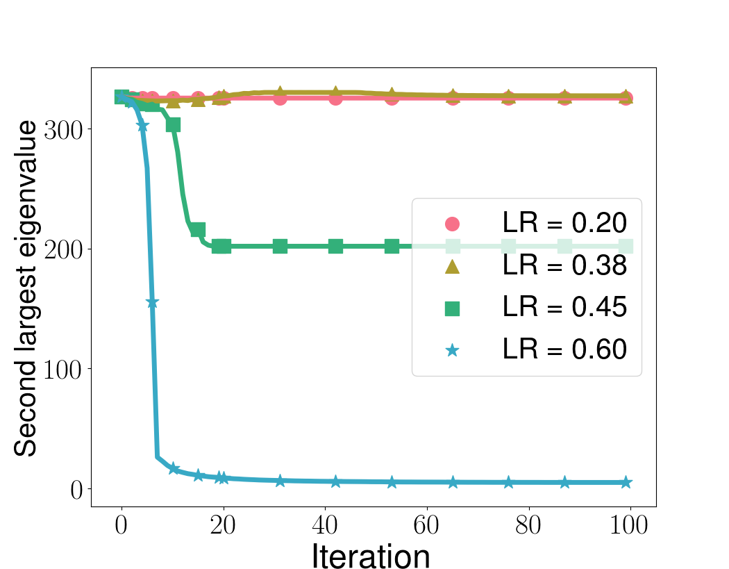
We verify the results for multiple training examples via the experiments in Figure 3.
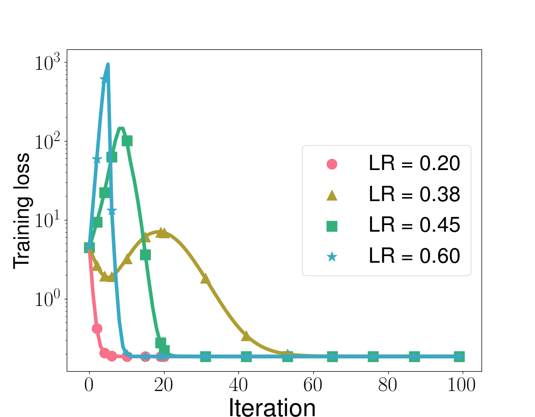
Refer to caption
(a) Training loss
Refer to caption
(b) Largest eigenvalue of tangent kernel
Refer to caption
(c) Second largest eigenvalue of tangent kernel
Figure 3: Training dynamics of NQMs for multiple examples case with different learning rates. By our analysis, two critical values are 2/λ1(0)=0.372subscript𝜆100.372/\lambda_{1}(0)=0.37 and 2/λ2(0)=0.392subscript𝜆200.392/\lambda_{2}(0)=0.39. When η<0.37𝜂0.37\eta<0.37, linear dynamics dominate hence the kernel is nearly constant; when 0.37<η<0.390.37𝜂0.390.37<\eta<0.39, the catapult phase happens in 𝒑1subscript𝒑1{\boldsymbol{p}}_{1} and only λ1(t)subscript𝜆1𝑡\lambda_{1}(t) decreases; when 0.39<η<ηmax0.39𝜂subscript𝜂max0.39<\eta<{\eta_{\mathrm{max}}}, the catapult phase happens in 𝒑1subscript𝒑1{\boldsymbol{p}}_{1} and 𝒑2subscript𝒑2{\boldsymbol{p}}_{2} hence both λ1(t)subscript𝜆1𝑡\lambda_{1}(t) and λ2(t)subscript𝜆2𝑡\lambda_{2}(t) decreases. The experiment details can be found in Appendix N.1.

3.3 Connection to general quadratic models and wide neural networks

General quadratic models.

As mentioned in the introduction, NQMs are contained in a general class of quadratic models of the form given in Eq. (3). Additionally, we show that the two-layer linear neural network analyzed in [15] is a special case of Eq. (3), and we provide a more general condition for such models to have catapult dynamics in Appendix M. Furthermore, we empirically observe that a broader class of quadratic models g𝑔g can have catapult dynamics simply by letting ϕ(𝒙)italic-ϕ𝒙\phi({\boldsymbol{x}}) and ΣΣ\Sigma be random and assigning a small value to γ𝛾\gamma (See Appendix N.4).

Wide neural networks.

We have seen that NQMs, with fixed Hessian, exhibit the catapult phase phenomenon. Therefore, the change in the Hessian of wide neural networks during training is not required to produce the catapult phase. We will discuss the high-level idea of analyzing the catapult phase for a general NQM with large learning rates, and empirically show that this idea applies to neural networks. We train an NQM Eq. (2) fquadsubscript𝑓quadf_{\mathrm{quad}} on n𝑛n data points {(𝒙i,yi)}i=1nd×superscriptsubscriptsubscript𝒙𝑖subscript𝑦𝑖𝑖1𝑛superscript𝑑\{({\boldsymbol{x}}_{i},y_{i})\}_{i=1}^{n}\in\mathbb{R}^{d}\times\mathbb{R} with GD. The dynamics equations take the following form:

𝐟quad(t+1)𝐲subscript𝐟quad𝑡1𝐲\displaystyle{\mathbf{f}}_{\mathrm{quad}}(t+1)-{\mathbf{y}} =(IηK(t)+12η2G(t)𝐟quad(t)TR𝐟quad(t))(𝐟quad(t)𝐲),absent𝐼𝜂𝐾𝑡subscript12superscript𝜂2𝐺𝑡subscript𝐟quadsuperscript𝑡𝑇subscript𝑅subscript𝐟quad𝑡subscript𝐟quad𝑡𝐲\displaystyle=\left(I-\eta K(t)+\underbrace{\frac{1}{2}\eta^{2}G(t)\nabla{\mathbf{f}}_{\mathrm{quad}}(t)^{T}}_{R_{{\mathbf{f}}_{\mathrm{quad}}}(t)}\right)({\mathbf{f}}_{\mathrm{quad}}(t)-{\mathbf{y}}), (15)
K(t+1)𝐾𝑡1\displaystyle K(t+1) =K(t)14η(4G(t)𝐟quad(t)TηG(t)G(t)T)RK(t),absent𝐾𝑡subscript14𝜂4𝐺𝑡subscript𝐟quadsuperscript𝑡𝑇𝜂𝐺𝑡𝐺superscript𝑡𝑇subscript𝑅𝐾𝑡\displaystyle=K(t)-\underbrace{\frac{1}{4}\eta\left(4G(t)\nabla{\mathbf{f}}_{\mathrm{quad}}(t)^{T}-\eta G(t)G(t)^{T}\right)}_{R_{K}(t)}, (16)

where Gi,:(t)=(𝐟quad(t)𝐲)T𝐟quad(t)Hf(𝒙i)msubscript𝐺𝑖:𝑡superscriptsubscript𝐟quad𝑡𝐲𝑇subscript𝐟quad𝑡subscript𝐻𝑓subscript𝒙𝑖superscript𝑚G_{i,:}(t)=({\mathbf{f}}_{\mathrm{quad}}(t)-{\mathbf{y}})^{T}\nabla{\mathbf{f}}_{\mathrm{quad}}(t)H_{f}({\boldsymbol{x}}_{i})\in\mathbb{R}^{m} for i[n]𝑖delimited-[]𝑛i\in[n].

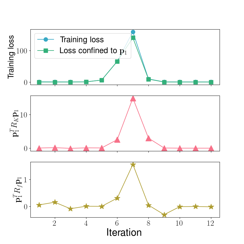
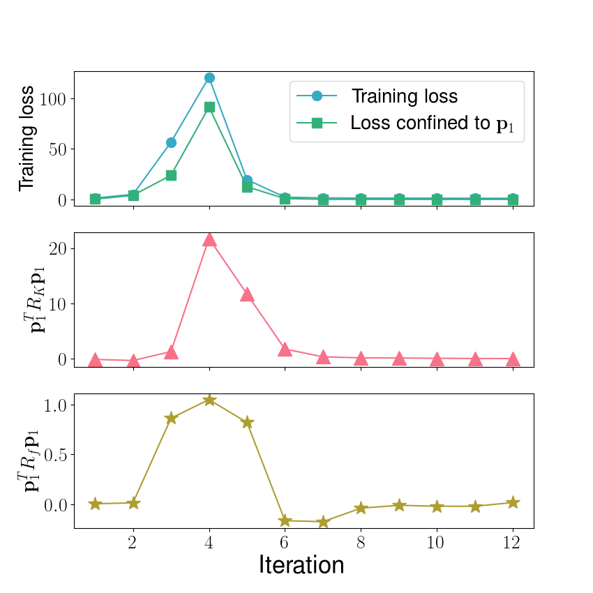
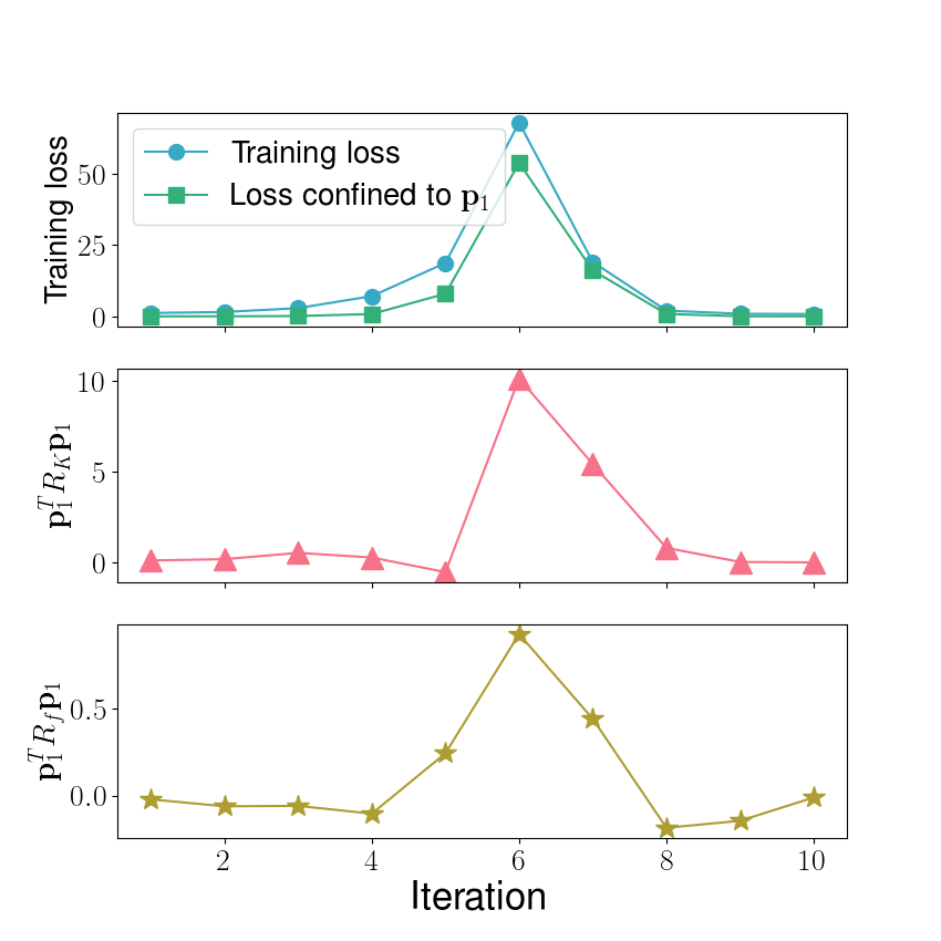
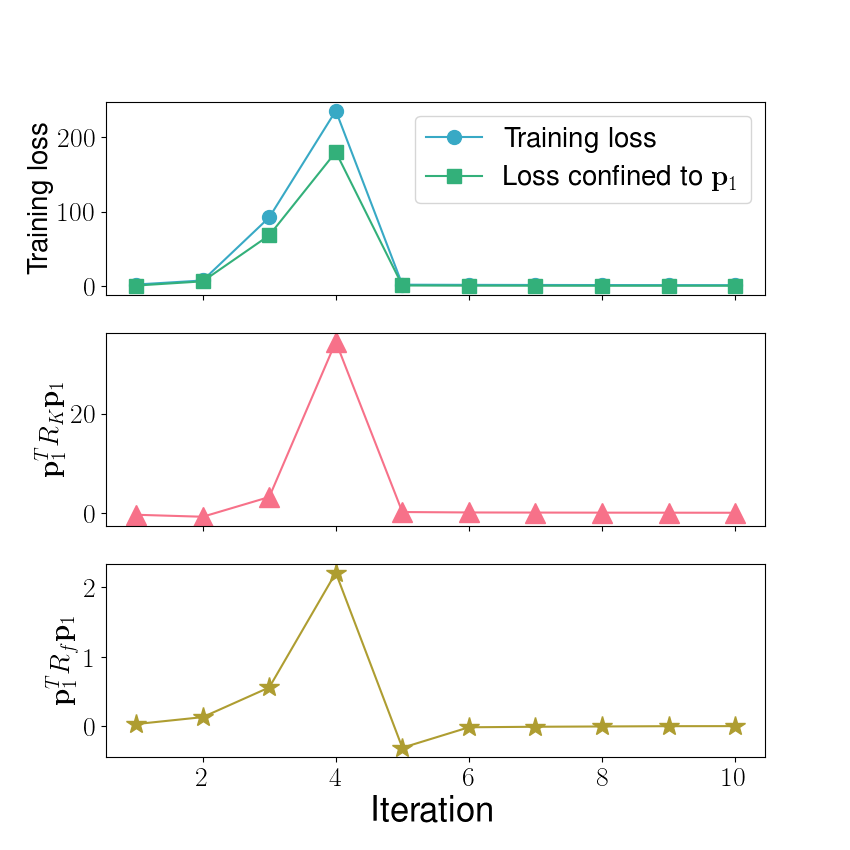
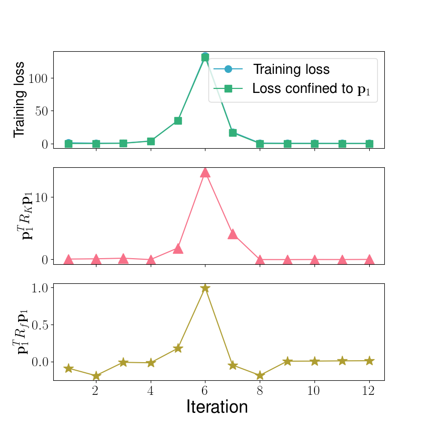
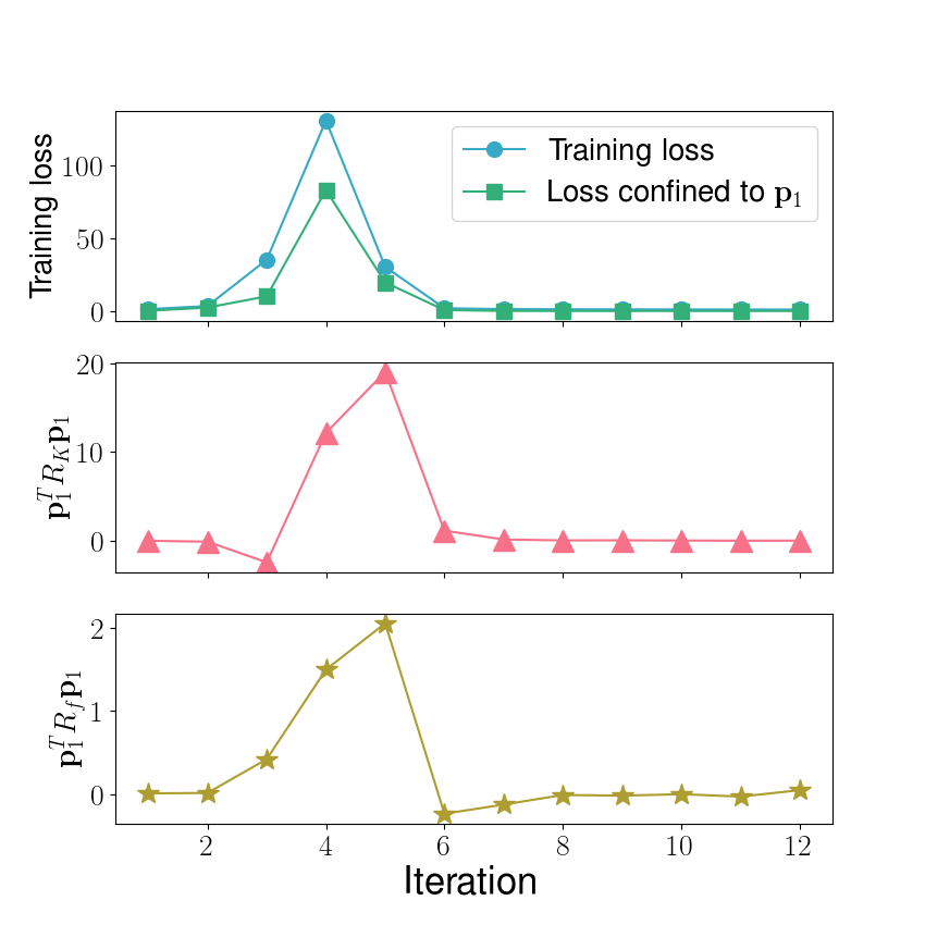
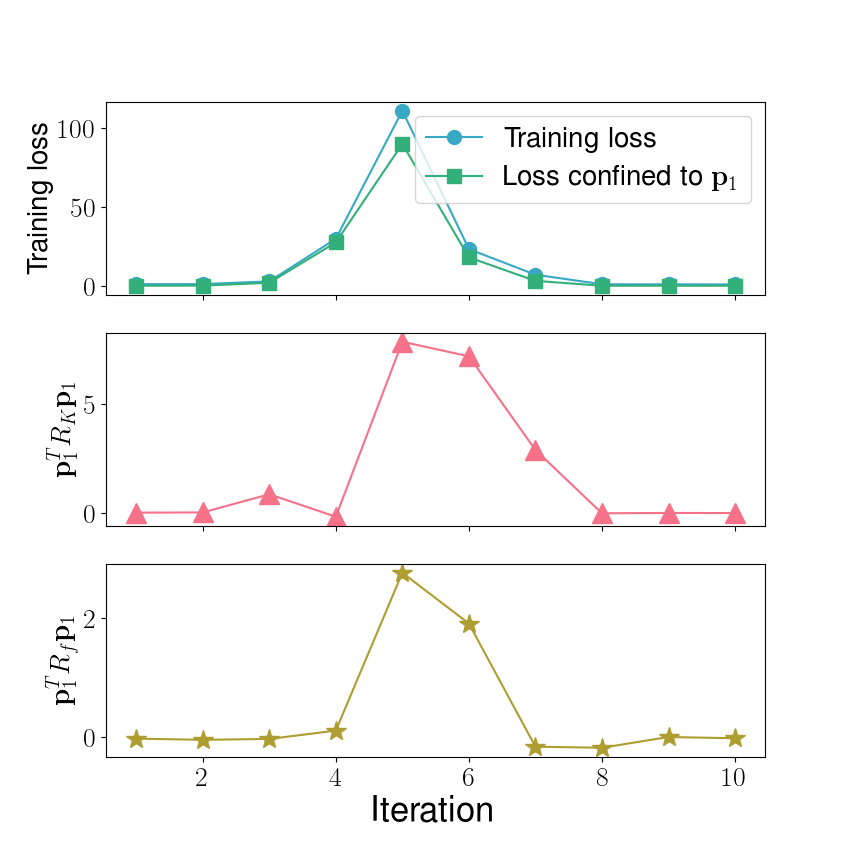
In our analysis for fquadsubscript𝑓quadf_{{\mathrm{quad}}} which approximates two-layer networks in Section 3.2, we show that catapult dynamics occur in the top eigenspace of the tangent kernel. Specifically, we analyze the dynamics equations confined to the top eigendirection of the tangent kernel 𝒑1subscript𝒑1{\boldsymbol{p}}_{1} (i.e, Π1subscriptΠ1\Pi_{1}{\mathcal{L}} and λ1(t)subscript𝜆1𝑡\lambda_{1}(t)). We show that 𝒑1TR𝐟quad𝒑1superscriptsubscript𝒑1𝑇subscript𝑅subscript𝐟quadsubscript𝒑1{\boldsymbol{p}}_{1}^{T}R_{{\mathbf{f}}_{\mathrm{quad}}}{\boldsymbol{p}}_{1} and 𝒑1TRK𝒑1superscriptsubscript𝒑1𝑇subscript𝑅𝐾subscript𝒑1{\boldsymbol{p}}_{1}^{T}R_{K}{\boldsymbol{p}}_{1} scale with the loss and remain positive when the loss becomes large, therefore 𝒑1TK𝒑1superscriptsubscript𝒑1𝑇𝐾subscript𝒑1{\boldsymbol{p}}_{1}^{T}K{\boldsymbol{p}}_{1} (i.e., λmax(K)subscript𝜆𝐾\lambda_{\max}(K)) as well as the loss will be driven down, and consequently we yield catapult convergence.

We empirically verify catapults indeed happen in the top eigenspace of the tangent kernel for additional NQMs and wide neural networks in Appendix N.3. Furthermore, a similar behaviour of top eigenvalues of the tangent kernel with the one for NQMs is observed for wide neural networks when training with different learning rates (See Figure 5 in Appendix N).

4 Quadratic models parallel neural networks in generalization

In this section, we empirically compare the test performance of three different models considered in this paper upon varying learning rate. In particular, we consider (1) the NQM, fquadsubscript𝑓quadf_{\mathrm{quad}}; (2) corresponding neural networks, f𝑓f; and (3) the linear model, flinsubscript𝑓linf_{\mathrm{lin}}.

Refer to caption
Refer to caption
Refer to caption
Refer to caption
Refer to caption
Refer to caption
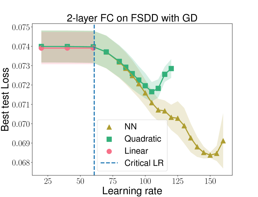
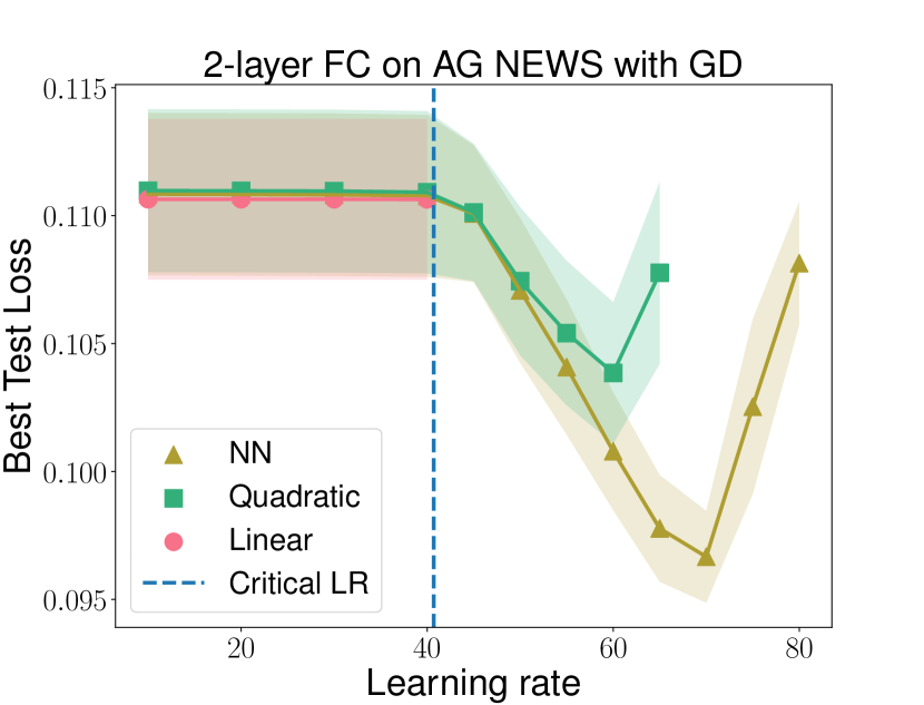
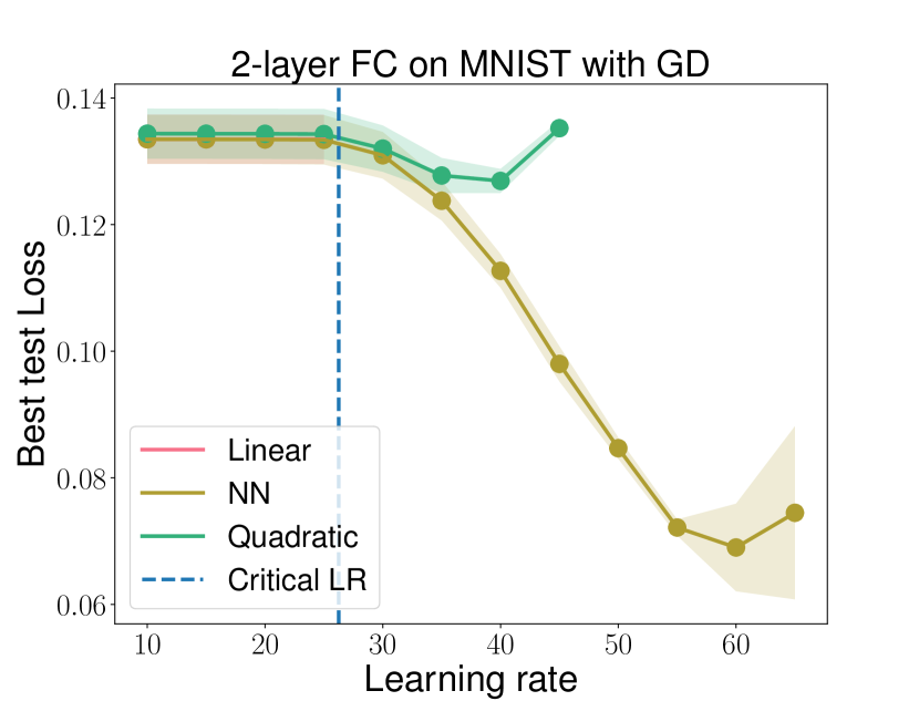
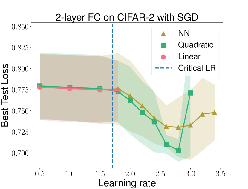
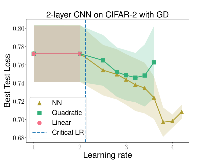
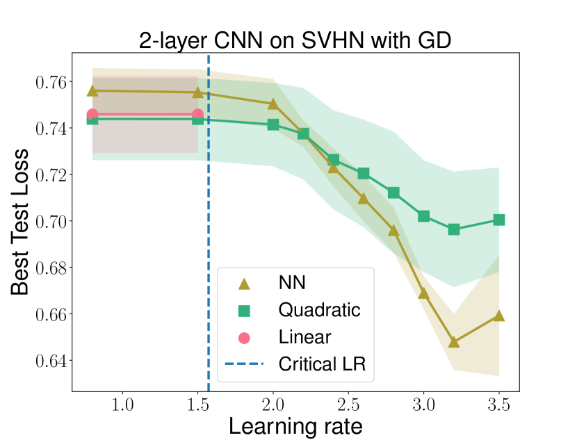
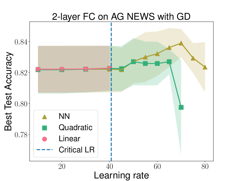
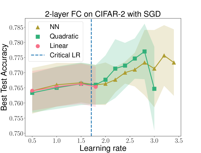
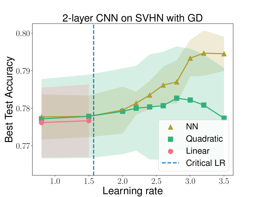
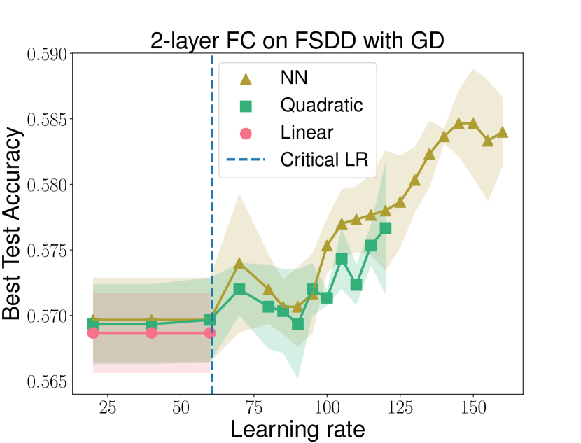
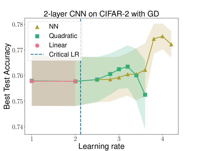
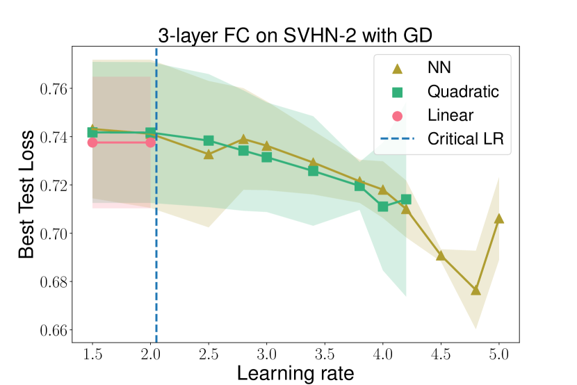
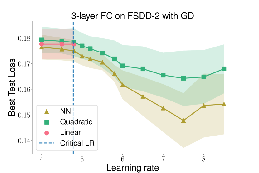
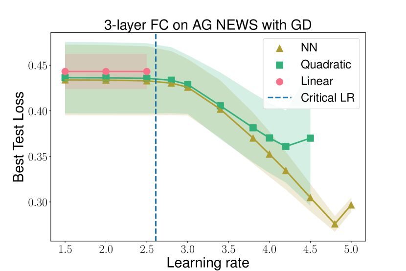
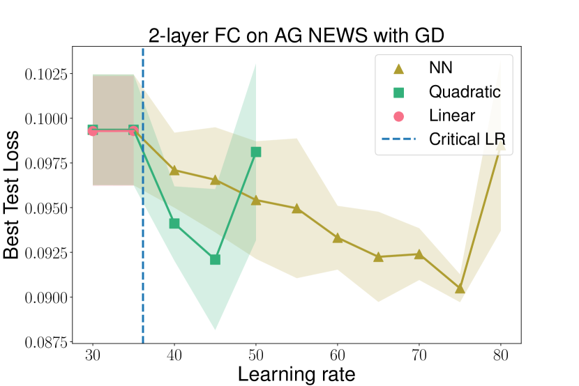
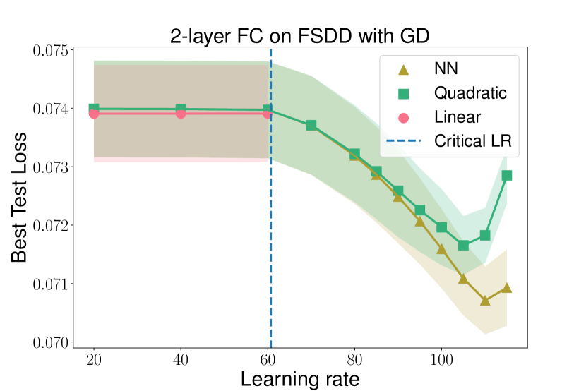
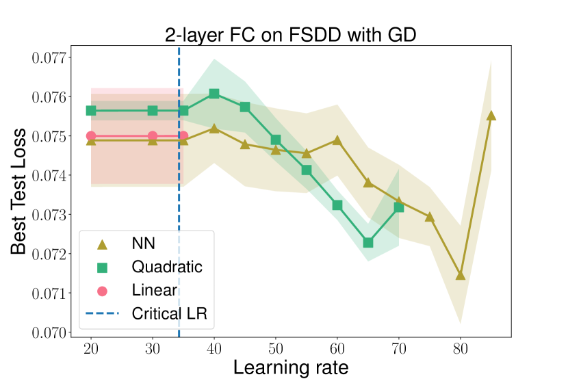
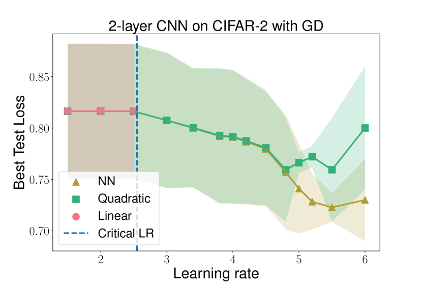
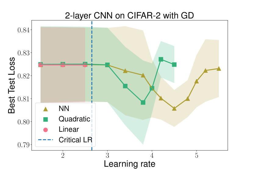
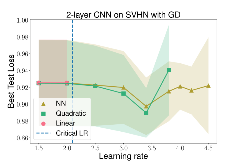
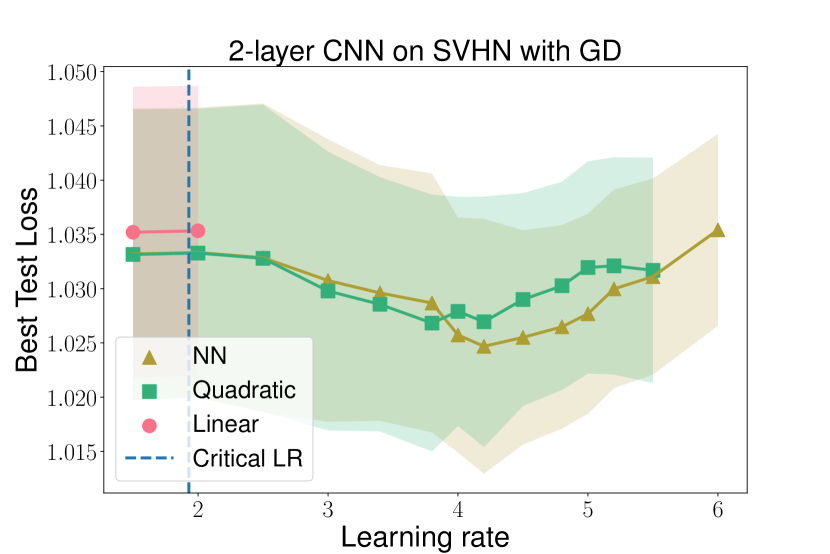
Figure 4: Best test loss plotted against different learning rates for f(𝐰)𝑓𝐰f({\mathbf{w}}), flin(𝐰)subscript𝑓lin𝐰f_{{{\mathrm{lin}}}}({\mathbf{w}}) and fquad(𝐰)subscript𝑓quad𝐰f_{{\mathrm{quad}}}({\mathbf{w}}) across a variety of datasets and network architectures.

We implement our experiments on 3 vision datasets: CIFAR-2 (a 2-class subset of CIFAR-10 [12]), MNIST [13], and SVHN (The Street View House Numbers) [19], 1 speech dataset: Free Spoken Digit dataset (FSDD) [10] and 1 text dataset: AG NEWS [7].

In all experiments, we train the models by minimizing the squared loss using standard GD/SGD with constant learning rate η𝜂\eta. We report the best test loss achieved during the training process with each learning rate. Experimental details can be found in Appendix N.5. We also report the best test accuracy in Appendix N.6. For networks with 333 layers, see Appendix N.7. From the experimental results, we observe the following:

Sub-critical learning rates.

In accordance with our theoretical analyses, we observe that all three models have nearly identical test loss for any sub-critical learning rate. Specifically, note that as the width m𝑚m increases, f𝑓f and fquadsubscript𝑓quadf_{{\mathrm{quad}}} will transition to linearity in the ball B(𝐰0,R)𝐵subscript𝐰0𝑅B({\mathbf{w}}_{0},R):

fflin=O~(1/m),fquadflin=O~(1/m),formulae-sequencenorm𝑓subscript𝑓lin~𝑂1𝑚normsubscript𝑓quadsubscript𝑓lin~𝑂1𝑚\displaystyle\|f-f_{{{\mathrm{lin}}}}\|=\tilde{O}(1/\sqrt{m}),~{}~{}~{}\|f_{{\mathrm{quad}}}-f_{{{\mathrm{lin}}}}\|=\tilde{O}(1/\sqrt{m}),

where R>0𝑅0R>0 is a constant which is large enough to contain the optimization path with respect to sub-critical learning rates. Thus, the generalization performance of these three models will be similar when m𝑚m is large, as shown in Figure 4.

Super-critical learning rates.

The best test loss of both f(𝐰)𝑓𝐰f({\mathbf{w}}) and fquad(𝐰)subscript𝑓quad𝐰f_{{\mathrm{quad}}}({\mathbf{w}}) is consistently smaller than the one with sub-critical learning rates, and decreases for an increasing learning rate in a range of values beyond ηcritsubscript𝜂crit{\eta_{\mathrm{crit}}}, which was observed for wide neural networks in [15].

As discussed in the introduction, with super-critical learning rates, both fquadsubscript𝑓quadf_{{\mathrm{quad}}} and f𝑓f can be observed to have catapult phase, while the loss of flinsubscript𝑓linf_{{{\mathrm{lin}}}} diverges. Together with the similar behaviour of fquadsubscript𝑓quadf_{{\mathrm{quad}}} and f𝑓f in generalization with super-critical learning rates, we believe NQMs are a better model to understand f𝑓f in training and testing dynamics, than the linear approximation flinsubscript𝑓linf_{{{\mathrm{lin}}}}.

In Figure 4 we report the results for networks with ReLU activation function. We also implement the experiments using networks with Tanh and Swish [23] activation functions, and observe the same phenomena in generalization for f𝑓f, flinsubscript𝑓linf_{{{\mathrm{lin}}}} and fquadsubscript𝑓quadf_{{\mathrm{quad}}} (See Appendix N.8).

5 Summary and Discussion

Summary.

In this paper, we use quadratic models as a tool to better understand optimization and generalization properties of finite width neural networks trained using large learning rates. Notably, we prove that quadratic models exhibit properties of neural networks such as the catapult phase that cannot be explained using linear models, which importantly includes linear approximations to neural networks given by the neural tangent kernel. Interestingly, we show empirically that quadratic models mimic the generalization properties of neural networks when trained with large learning rate, and that such models perform better than linearized neural networks.

Future directions.

As quadratic models are more analytically tractable than finite width neural networks, these models open further avenues for understanding the good performance of finite width networks in practice. In particular, one interesting direction of future work is to understand the change in the kernel corresponding to a trained quadratic model. As we showed, training a quadratic model with large learning rate causes a decrease in the eigenvalues of the neural tangent kernel, and it would be interesting to understand the properties of this changed kernel that correspond with improved generalization. Indeed, prior work [17] has analyzed the properties of the “after kernel” corresponding to finite width neural networks, and it would be interesting to observe whether similar properties hold for the kernel corresponding to trained quadratic models.

Another interesting avenue of research is to understand whether quadratic models can be used for representation learning. Indeed, prior work [27] argues that networks in the neural tangent kernel regime do not learn useful representations of data through training. As quadratic models trained with large learning rate can already exhibit nonlinear dynamics and better capture generalization properties of finite width networks, it would be interesting to understand whether such models learn useful representations of data as well.

Acknowledgements

We thank Boris Hanin, Daniel A. Roberts and Sho Yaida for the discussion about quadratic models and catapults. A.R. is supported by the Eric and Wendy Schmidt Center at the Broad Institute. We are grateful for the support from the National Science Foundation (NSF) and the Simons Foundation for the Collaboration on the Theoretical Foundations of Deep Learning (https://deepfoundations.ai/) through awards DMS-2031883 and #814639 and the TILOS institute (NSF CCF-2112665). This work used NVIDIA V100 GPUs NVLINK and HDR IB (Expanse GPU) at SDSC Dell Cluster through allocation TG-CIS220009 and also, Delta system at the National Center for Supercomputing Applications through allocation bbjr-delta-gpu from the Advanced Cyberinfrastructure Coordination Ecosystem: Services & Support (ACCESS) program, which is supported by National Science Foundation grants #2138259, #2138286, #2138307, #2137603, and #2138296.

References

  • [1] Yu Bai and Jason D Lee “Beyond Linearization: On Quadratic and Higher-Order Approximation of Wide Neural Networks” In International Conference on Learning Representations, 2019
  • [2] Nicoletta Bof, Ruggero Carli and Luca Schenato “Lyapunov theory for discrete time systems” In arXiv preprint arXiv:1809.05289, 2018
  • [3] Lenaic Chizat, Edouard Oyallon and Francis Bach “On lazy training in differentiable programming” In Advances in Neural Information Processing Systems 32, 2019
  • [4] Simon Du, Jason Lee, Haochuan Li, Liwei Wang and Xiyu Zhai “Gradient Descent Finds Global Minima of Deep Neural Networks” In International Conference on Machine Learning, 2019, pp. 1675–1685
  • [5] Simon S Du, Xiyu Zhai, Barnabas Poczos and Aarti Singh “Gradient descent provably optimizes over-parameterized neural networks” In arXiv preprint arXiv:1810.02054, 2018
  • [6] Stanislav Fort, Gintare Karolina Dziugaite, Mansheej Paul, Sepideh Kharaghani, Daniel M Roy and Surya Ganguli “Deep learning versus kernel learning: an empirical study of loss landscape geometry and the time evolution of the neural tangent kernel” In Advances in Neural Information Processing Systems 33, 2020, pp. 5850–5861
  • [7] Antonio Gulli “AG’s corpus of news articles” http://groups.di.unipi.it/~gulli/AG_corpus_of_news_articles.html
  • [8] Jiaoyang Huang and Horng-Tzer Yau “Dynamics of deep neural networks and neural tangent hierarchy” In International Conference on Machine Learning, 2020, pp. 4542–4551 PMLR
  • [9] Arthur Jacot, Franck Gabriel and Clément Hongler “Neural tangent kernel: Convergence and generalization in neural networks” In Advances in neural information processing systems, 2018, pp. 8571–8580
  • [10] Jakobovski “Free-Spoken-Digit-Dataset” https://github.com/Jakobovski/free-spoken-digit-dataset
  • [11] Ziwei Ji and Matus Telgarsky “Polylogarithmic width suffices for gradient descent to achieve arbitrarily small test error with shallow ReLU networks” In International Conference on Learning Representations, 2019
  • [12] Alex Krizhevsky and Geoffrey Hinton “Learning multiple layers of features from tiny images” Citeseer, 2009
  • [13] Yann LeCun, Léon Bottou, Yoshua Bengio and Patrick Haffner “Gradient-based learning applied to document recognition” In Proceedings of the IEEE 86.11 Ieee, 1998, pp. 2278–2324
  • [14] Jaehoon Lee, Lechao Xiao, Samuel Schoenholz, Yasaman Bahri, Roman Novak, Jascha Sohl-Dickstein and Jeffrey Pennington “Wide neural networks of any depth evolve as linear models under gradient descent” In Advances in neural information processing systems, 2019, pp. 8570–8581
  • [15] Aitor Lewkowycz, Yasaman Bahri, Ethan Dyer, Jascha Sohl-Dickstein and Guy Gur-Ari “The large learning rate phase of deep learning: the catapult mechanism” In arXiv preprint arXiv:2003.02218, 2020
  • [16] Chaoyue Liu, Libin Zhu and Mikhail Belkin “On the linearity of large non-linear models: when and why the tangent kernel is constant” In Advances in Neural Information Processing Systems 33, 2020
  • [17] Philip M Long “Properties of the After Kernel” In arXiv preprint arXiv:2105.10585, 2021
  • [18] Andrea Montanari and Yiqiao Zhong “The interpolation phase transition in neural networks: Memorization and generalization under lazy training” In arXiv preprint arXiv:2007.12826, 2020
  • [19] Yuval Netzer, Tao Wang, Adam Coates, Alessandro Bissacco, Bo Wu and Andrew Y Ng “Reading digits in natural images with unsupervised feature learning”, 2011
  • [20] Eshaan Nichani, Adityanarayanan Radhakrishnan and Caroline Uhler “Increasing Depth Leads to U-Shaped Test Risk in Over-parameterized Convolutional Networks” In International Conference on Machine Learning Workshop on Over-parameterization: Pitfalls and Opportunities, 2021
  • [21] Guillermo Ortiz-Jiménez, Seyed-Mohsen Moosavi-Dezfooli and Pascal Frossard “What can linearized neural networks actually say about generalization?” In Advances in Neural Information Processing Systems 34, 2021
  • [22] Boris T Polyak “Introduction to optimization” In Optimization Software, Inc, New York, 1987
  • [23] Prajit Ramachandran, Barret Zoph and Quoc V Le “Searching for activation functions” In arXiv preprint arXiv:1710.05941, 2017
  • [24] Daniel A Roberts, Sho Yaida and Boris Hanin “The principles of deep learning theory” Cambridge University Press, 2022
  • [25] Pedro Savarese, Itay Evron, Daniel Soudry and Nathan Srebro “How do infinite width bounded norm networks look in function space?” In Conference on Learning Theory, 2019, pp. 2667–2690 PMLR
  • [26] Francis Williams, Matthew Trager, Daniele Panozzo, Claudio Silva, Denis Zorin and Joan Bruna “Gradient dynamics of shallow univariate relu networks” In Advances in Neural Information Processing Systems 32, 2019
  • [27] Greg Yang and Edward J Hu “Feature learning in infinite-width neural networks” In arXiv preprint arXiv:2011.14522, 2020
  • [28] Guodong Zhang, Lala Li, Zachary Nado, James Martens, Sushant Sachdeva, George Dahl, Chris Shallue and Roger B Grosse “Which algorithmic choices matter at which batch sizes? insights from a noisy quadratic model” In Advances in neural information processing systems 32, 2019
  • [29] Difan Zou and Quanquan Gu “An improved analysis of training over-parameterized deep neural networks” In Advances in Neural Information Processing Systems, 2019, pp. 2053–2062

Appendix A Derivation of NQM

We will derive the NQM that approximate the two-layer fully connected ReLU activated neural networks based on Eq. (2).

The first derivative of f𝑓f can be computed by:

f𝐮i=1mdvi𝟙{𝐮iT𝒙0}𝒙T,fvi=1mσ(1d𝐮iT𝒙),i[m].formulae-sequence𝑓subscript𝐮𝑖1𝑚𝑑subscript𝑣𝑖subscript1superscriptsubscript𝐮𝑖𝑇𝒙0superscript𝒙𝑇formulae-sequence𝑓subscript𝑣𝑖1𝑚𝜎1𝑑superscriptsubscript𝐮𝑖𝑇𝒙for-all𝑖delimited-[]𝑚\displaystyle\frac{\partial f}{\partial{\mathbf{u}}_{i}}=\frac{1}{\sqrt{md}}v_{i}\mathbbm{1}_{\left\{{\mathbf{u}}_{i}^{T}{\boldsymbol{x}}\geq 0\right\}}{\boldsymbol{x}}^{T},~{}~{}~{}~{}\frac{\partial f}{\partial v_{i}}=\frac{1}{\sqrt{m}}\sigma\left(\frac{1}{\sqrt{d}}{\mathbf{u}}_{i}^{T}{\boldsymbol{x}}\right),~{}~{}~{}\forall i\in[m].

And each entry of the Hessian of f𝑓f, i.e., Hfsubscript𝐻𝑓H_{f}, can be computed by

2f𝐮i2=𝟎,2fvi2=0,2f𝐮ivi=1md𝟙{𝐮iT𝒙0}𝒙T,i[m].formulae-sequencesuperscript2𝑓superscriptsubscript𝐮𝑖20formulae-sequencesuperscript2𝑓superscriptsubscript𝑣𝑖20formulae-sequencesuperscript2𝑓subscript𝐮𝑖subscript𝑣𝑖1𝑚𝑑subscript1superscriptsubscript𝐮𝑖𝑇𝒙0superscript𝒙𝑇for-all𝑖delimited-[]𝑚\displaystyle\frac{\partial^{2}f}{\partial{\mathbf{u}}_{i}^{2}}=\mathbf{0},~{}~{}\frac{\partial^{2}f}{\partial v_{i}^{2}}=0,~{}~{}~{}\frac{\partial^{2}f}{\partial{\mathbf{u}}_{i}v_{i}}=\frac{1}{\sqrt{md}}\mathbbm{1}_{\left\{{\mathbf{u}}_{i}^{T}{\boldsymbol{x}}\geq 0\right\}}{\boldsymbol{x}}^{T},~{}~{}~{}~{}\forall i\in[m].

Now we get fquadsubscript𝑓quadf_{{\mathrm{quad}}} taking the following form

𝐍𝐐𝐌:fquad(𝐮,𝐯;𝒙):𝐍𝐐𝐌subscript𝑓quad𝐮𝐯𝒙\displaystyle\mathbf{NQM:}~{}~{}f_{\mathrm{quad}}({\mathbf{u}},{\mathbf{v}};{\boldsymbol{x}}) =f(𝐮0,𝐯0;𝒙)+1mdi=1m(𝐮i𝐮0,i)T𝒙𝟙{𝐮0,iT𝒙0}v0,i+1mi=1m(viv0,i)σ(1d𝐮0,iT𝒙)absent𝑓subscript𝐮0subscript𝐯0𝒙1𝑚𝑑superscriptsubscript𝑖1𝑚superscriptsubscript𝐮𝑖subscript𝐮0𝑖𝑇𝒙subscript1superscriptsubscript𝐮0𝑖𝑇𝒙0subscript𝑣0𝑖1𝑚superscriptsubscript𝑖1𝑚subscript𝑣𝑖subscript𝑣0𝑖𝜎1𝑑superscriptsubscript𝐮0𝑖𝑇𝒙\displaystyle=f({\mathbf{u}}_{0},{\mathbf{v}}_{0};{\boldsymbol{x}})+\frac{1}{\sqrt{md}}\sum_{i=1}^{m}({\mathbf{u}}_{i}-{\mathbf{u}}_{0,i})^{T}{\boldsymbol{x}}\mathbbm{1}_{\left\{{\mathbf{u}}_{0,i}^{T}{\boldsymbol{x}}\geq 0\right\}}v_{0,i}+\frac{1}{\sqrt{m}}\sum_{i=1}^{m}(v_{i}-v_{0,i})\sigma\left(\frac{1}{\sqrt{d}}{\mathbf{u}}_{0,i}^{T}{\boldsymbol{x}}\right)
+1mdi=1m(𝐮i𝐮0,i)T𝒙𝟙{𝐮0,iT𝒙0}(viv0,i).1𝑚𝑑superscriptsubscript𝑖1𝑚superscriptsubscript𝐮𝑖subscript𝐮0𝑖𝑇𝒙subscript1superscriptsubscript𝐮0𝑖𝑇𝒙0subscript𝑣𝑖subscript𝑣0𝑖\displaystyle~{}~{}~{}~{}+\frac{1}{\sqrt{md}}\sum_{i=1}^{m}({\mathbf{u}}_{i}-{\mathbf{u}}_{0,i})^{T}{\boldsymbol{x}}\mathbbm{1}_{\left\{{\mathbf{u}}_{0,i}^{T}{\boldsymbol{x}}\geq 0\right\}}(v_{i}-v_{0,i}). (17)

Appendix B Derivation of dynamics equations

B.1 Single training example

The NQM can be equivalently written as:

g(𝐮,𝐯;𝒙)𝑔𝐮𝐯𝒙\displaystyle g({\mathbf{u}},{\mathbf{v}};{\boldsymbol{x}}) =g(𝐮0,𝐯0;𝒙)+𝐮𝐮0,𝐮g(𝐮,𝐯;𝒙)|𝐮=𝐮0,𝐯=𝐯0+𝐯𝐯0,𝐯g(𝐮,𝐯;𝒙)|𝐮=𝐮0,𝐯=𝐯0absent𝑔subscript𝐮0subscript𝐯0𝒙𝐮subscript𝐮0evaluated-atsubscript𝐮𝑔𝐮𝐯𝒙formulae-sequence𝐮subscript𝐮0𝐯subscript𝐯0𝐯subscript𝐯0evaluated-atsubscript𝐯𝑔𝐮𝐯𝒙formulae-sequence𝐮subscript𝐮0𝐯subscript𝐯0\displaystyle=g({\mathbf{u}}_{0},{\mathbf{v}}_{0};{\boldsymbol{x}})+\left<{\mathbf{u}}-{\mathbf{u}}_{0},\evaluated{\nabla_{{\mathbf{u}}}g({\mathbf{u}},{\mathbf{v}};{\boldsymbol{x}})}_{{\mathbf{u}}={\mathbf{u}}_{0},{\mathbf{v}}={\mathbf{v}}_{0}}\right>+\left<{\mathbf{v}}-{\mathbf{v}}_{0},\evaluated{\nabla_{{\mathbf{v}}}g({\mathbf{u}},{\mathbf{v}};{\boldsymbol{x}})}_{{\mathbf{u}}={\mathbf{u}}_{0},{\mathbf{v}}={\mathbf{v}}_{0}}\right>
+𝐮𝐮0,2g(𝐮,𝐯;𝒙)𝐮𝐯|𝐮=𝐮0,𝐯=𝐯0(𝐯𝐯0),𝐮subscript𝐮0evaluated-atsuperscript2𝑔𝐮𝐯𝒙𝐮𝐯formulae-sequence𝐮subscript𝐮0𝐯subscript𝐯0𝐯subscript𝐯0\displaystyle~{}~{}~{}~{}+\left<{\mathbf{u}}-{\mathbf{u}}_{0},\evaluated{\frac{\partial^{2}g({\mathbf{u}},{\mathbf{v}};{\boldsymbol{x}})}{\partial{\mathbf{u}}\partial{\mathbf{v}}}}_{{\mathbf{u}}={\mathbf{u}}_{0},{\mathbf{v}}={\mathbf{v}}_{0}}({\mathbf{v}}-{\mathbf{v}}_{0})\right>,

since 2g𝐮2=0superscript2𝑔superscript𝐮20\frac{\partial^{2}g}{\partial{\mathbf{u}}^{2}}=0 and 2g𝐯2=0superscript2𝑔superscript𝐯20\frac{\partial^{2}g}{\partial{\mathbf{v}}^{2}}=0.

And the tangent kernel λ(𝐮,𝐯;𝒙)𝜆𝐮𝐯𝒙\lambda({\mathbf{u}},{\mathbf{v}};{\boldsymbol{x}}) takes the form

λ(𝐮,𝐯;𝒙)𝜆𝐮𝐯𝒙\displaystyle\lambda({\mathbf{u}},{\mathbf{v}};{\boldsymbol{x}}) =𝐮g(𝐮,𝐯;𝒙)|𝐮=𝐮0,𝐯=𝐯0+2g(𝐮,𝐯;𝒙)𝐮𝐯|𝐮=𝐮0(𝐯𝐯0)F2absentsuperscriptsubscriptnormevaluated-atsubscript𝐮𝑔𝐮𝐯𝒙formulae-sequence𝐮subscript𝐮0𝐯subscript𝐯0evaluated-atsuperscript2𝑔𝐮𝐯𝒙𝐮𝐯𝐮subscript𝐮0𝐯subscript𝐯0𝐹2\displaystyle=\norm{\evaluated{\nabla_{{\mathbf{u}}}g({\mathbf{u}},{\mathbf{v}};{\boldsymbol{x}})}_{{\mathbf{u}}={\mathbf{u}}_{0},{\mathbf{v}}={\mathbf{v}}_{0}}+\evaluated{\frac{\partial^{2}g({\mathbf{u}},{\mathbf{v}};{\boldsymbol{x}})}{\partial{\mathbf{u}}\partial{\mathbf{v}}}}_{{\mathbf{u}}={\mathbf{u}}_{0}}({\mathbf{v}}-{\mathbf{v}}_{0})}_{F}^{2}
+𝐯g(𝐮,𝐯;𝒙)|𝐮=𝐮0,𝐯=𝐯0+(𝐮𝐮0)T2g(𝐮,𝐯;𝒙)𝐮𝐯|𝐮=𝐮0,𝐯=𝐯02.superscriptnormevaluated-atsubscript𝐯𝑔𝐮𝐯𝒙formulae-sequence𝐮subscript𝐮0𝐯subscript𝐯0superscript𝐮subscript𝐮0𝑇evaluated-atsuperscript2𝑔𝐮𝐯𝒙𝐮𝐯formulae-sequence𝐮subscript𝐮0𝐯subscript𝐯02\displaystyle~{}~{}~{}~{}+\norm{\evaluated{\nabla_{{\mathbf{v}}}g({\mathbf{u}},{\mathbf{v}};{\boldsymbol{x}})}_{{\mathbf{u}}={\mathbf{u}}_{0},{\mathbf{v}}={\mathbf{v}}_{0}}+({\mathbf{u}}-{\mathbf{u}}_{0})^{T}\evaluated{\frac{\partial^{2}g({\mathbf{u}},{\mathbf{v}};{\boldsymbol{x}})}{\partial{\mathbf{u}}\partial{\mathbf{v}}}}_{{\mathbf{u}}={\mathbf{u}}_{0},{\mathbf{v}}={\mathbf{v}}_{0}}}^{2}.

Here

𝐮ig(𝐮,𝐯;𝒙)|𝐮=𝐮0,𝐯=𝐯0evaluated-atsubscriptsubscript𝐮𝑖𝑔𝐮𝐯𝒙formulae-sequence𝐮subscript𝐮0𝐯subscript𝐯0\displaystyle\evaluated{\nabla_{{\mathbf{u}}_{i}}g({\mathbf{u}},{\mathbf{v}};{\boldsymbol{x}})}_{{\mathbf{u}}={\mathbf{u}}_{0},{\mathbf{v}}={\mathbf{v}}_{0}} =1mdi=1mv0,i𝟙{𝐮0,iT𝒙0}𝒙,i[m],formulae-sequenceabsent1𝑚𝑑superscriptsubscript𝑖1𝑚subscript𝑣0𝑖subscript1superscriptsubscript𝐮0𝑖𝑇𝒙0𝒙for-all𝑖delimited-[]𝑚\displaystyle=\frac{1}{\sqrt{md}}\sum_{i=1}^{m}v_{0,i}\mathbbm{1}_{\left\{{\mathbf{u}}_{0,i}^{T}{\boldsymbol{x}}\geq 0\right\}}{\boldsymbol{x}},~{}~{}~{}\forall i\in[m],
𝐯g(𝐮,𝐯;𝒙)|𝐮=𝐮0,𝐯=𝐯0evaluated-atsubscript𝐯𝑔𝐮𝐯𝒙formulae-sequence𝐮subscript𝐮0𝐯subscript𝐯0\displaystyle\evaluated{\nabla_{{\mathbf{v}}}g({\mathbf{u}},{\mathbf{v}};{\boldsymbol{x}})}_{{\mathbf{u}}={\mathbf{u}}_{0},{\mathbf{v}}={\mathbf{v}}_{0}} =1mdσ(𝐮0T𝒙).absent1𝑚𝑑𝜎superscriptsubscript𝐮0𝑇𝒙\displaystyle=\frac{1}{\sqrt{md}}\sigma\left({\mathbf{u}}_{0}^{T}{\boldsymbol{x}}\right).

In the following, we will consider the dynamics of g𝑔g and λ𝜆\lambda with GD, hence for simplicity of notations, we denote

𝐮g(0)subscript𝐮𝑔0\displaystyle\nabla_{\mathbf{u}}g(0) :=𝐮g(𝐮,𝐯;𝒙)|𝐮=𝐮0,𝐯=𝐯0,assignabsentevaluated-atsubscript𝐮𝑔𝐮𝐯𝒙formulae-sequence𝐮subscript𝐮0𝐯subscript𝐯0\displaystyle:=\evaluated{\nabla_{{\mathbf{u}}}g({\mathbf{u}},{\mathbf{v}};{\boldsymbol{x}})}_{{\mathbf{u}}={\mathbf{u}}_{0},{\mathbf{v}}={\mathbf{v}}_{0}},
𝐯g(0)subscript𝐯𝑔0\displaystyle\nabla_{\mathbf{v}}g(0) :=𝐯g(𝐮,𝐯;𝒙)|𝐮=𝐮0,𝐯=𝐯0,assignabsentevaluated-atsubscript𝐯𝑔𝐮𝐯𝒙formulae-sequence𝐮subscript𝐮0𝐯subscript𝐯0\displaystyle:=\evaluated{\nabla_{{\mathbf{v}}}g({\mathbf{u}},{\mathbf{v}};{\boldsymbol{x}})}_{{\mathbf{u}}={\mathbf{u}}_{0},{\mathbf{v}}={\mathbf{v}}_{0}},
2g(0)𝐮𝐯superscript2𝑔0𝐮𝐯\displaystyle\frac{\partial^{2}g(0)}{\partial{\mathbf{u}}\partial{\mathbf{v}}} :=2g(𝐮,𝐯;𝒙)𝐮𝐯|𝐮=𝐮0,𝐯=𝐯0.assignabsentevaluated-atsuperscript2𝑔𝐮𝐯𝒙𝐮𝐯formulae-sequence𝐮subscript𝐮0𝐯subscript𝐯0\displaystyle:=\evaluated{\frac{\partial^{2}g({\mathbf{u}},{\mathbf{v}};{\boldsymbol{x}})}{\partial{\mathbf{u}}\partial{\mathbf{v}}}}_{{\mathbf{u}}={\mathbf{u}}_{0},{\mathbf{v}}={\mathbf{v}}_{0}}.

By gradient descent with learning rate η𝜂\eta, at iteration t𝑡t, we have the update equations for weights 𝐮𝐮{\mathbf{u}} and 𝐯𝐯{\mathbf{v}}:

𝐮(t+1)𝐮𝑡1\displaystyle{\mathbf{u}}(t+1) =𝐮(t)η(g(t)y)(𝐮g(0)+2g(0)𝐮𝐯(𝐯(t)𝐯(0))),absent𝐮𝑡𝜂𝑔𝑡𝑦subscript𝐮𝑔0superscript2𝑔0𝐮𝐯𝐯𝑡𝐯0\displaystyle={\mathbf{u}}(t)-\eta(g(t)-y)\left(\nabla_{{\mathbf{u}}}g(0)+\frac{\partial^{2}g(0)}{\partial{\mathbf{u}}\partial{\mathbf{v}}}({\mathbf{v}}(t)-{\mathbf{v}}(0))\right),
𝐯(t+1)𝐯𝑡1\displaystyle{\mathbf{v}}(t+1) =𝐯(t)η(g(t)y)(𝐯g(0)+(𝐮(t)𝐮(0))T2g(0)𝐮𝐯).absent𝐯𝑡𝜂𝑔𝑡𝑦subscript𝐯𝑔0superscript𝐮𝑡𝐮0𝑇superscript2𝑔0𝐮𝐯\displaystyle={\mathbf{v}}(t)-\eta(g(t)-y)\left(\nabla_{{\mathbf{v}}}g(0)+({\mathbf{u}}(t)-{\mathbf{u}}(0))^{T}\frac{\partial^{2}g(0)}{\partial{\mathbf{u}}\partial{\mathbf{v}}}\right).

Then we plug them in the expression of λ(t+1)𝜆𝑡1\lambda(t+1) and we get

λ(t+1)𝜆𝑡1\displaystyle\lambda(t+1) =𝐮g(0)+2g(0)𝐮𝐯(𝐯(t+1)𝐯(0))F2+𝐯g(0)+(𝐮(t+1)𝐮(0))T2g(0)𝐮𝐯2absentsuperscriptsubscriptnormsubscript𝐮𝑔0superscript2𝑔0𝐮𝐯𝐯𝑡1𝐯0𝐹2superscriptnormsubscript𝐯𝑔0superscript𝐮𝑡1𝐮0𝑇superscript2𝑔0𝐮𝐯2\displaystyle=\norm{\nabla_{{\mathbf{u}}}g(0)+\frac{\partial^{2}g(0)}{\partial{\mathbf{u}}\partial{\mathbf{v}}}({\mathbf{v}}(t+1)-{\mathbf{v}}(0))}_{F}^{2}+\norm{\nabla_{{\mathbf{v}}}g(0)+({\mathbf{u}}(t+1)-{\mathbf{u}}(0))^{T}\frac{\partial^{2}g(0)}{\partial{\mathbf{u}}\partial{\mathbf{v}}}}^{2}
=𝐮g(0)+2g(0)𝐮𝐯(𝐯(t)η(g(t)y)(𝐯g(0)+(𝐮(t)𝐮(0))T2g(0)𝐮𝐯)𝐯(0))F2absentsuperscriptsubscriptnormsubscript𝐮𝑔0superscript2𝑔0𝐮𝐯𝐯𝑡𝜂𝑔𝑡𝑦subscript𝐯𝑔0superscript𝐮𝑡𝐮0𝑇superscript2𝑔0𝐮𝐯𝐯0𝐹2\displaystyle=\norm{\nabla_{{\mathbf{u}}}g(0)+\frac{\partial^{2}g(0)}{\partial{\mathbf{u}}\partial{\mathbf{v}}}\left({\mathbf{v}}(t)-\eta(g(t)-y)\left(\nabla_{{\mathbf{v}}}g(0)+({\mathbf{u}}(t)-{\mathbf{u}}(0))^{T}\frac{\partial^{2}g(0)}{\partial{\mathbf{u}}\partial{\mathbf{v}}}\right)-{\mathbf{v}}(0)\right)}_{F}^{2}
+𝐯g(0)+(𝐮(t)η(g(t)y)(𝐮g(0)+2g(0)𝐮𝐯(𝐯(t)𝐯(0)))𝐮(0))T2g(0)𝐮𝐯2superscriptnormsubscript𝐯𝑔0superscript𝐮𝑡𝜂𝑔𝑡𝑦subscript𝐮𝑔0superscript2𝑔0𝐮𝐯𝐯𝑡𝐯0𝐮0𝑇superscript2𝑔0𝐮𝐯2\displaystyle~{}~{}~{}~{}+\norm{\nabla_{{\mathbf{v}}}g(0)+\left({\mathbf{u}}(t)-\eta(g(t)-y)\left(\nabla_{{\mathbf{u}}}g(0)+\frac{\partial^{2}g(0)}{\partial{\mathbf{u}}\partial{\mathbf{v}}}({\mathbf{v}}(t)-{\mathbf{v}}(0))\right)-{\mathbf{u}}(0)\right)^{T}\frac{\partial^{2}g(0)}{\partial{\mathbf{u}}\partial{\mathbf{v}}}}^{2}
=λ(t)+η2(g(t)y)22g(0)𝐮𝐯(𝐯g(0)+(𝐮(t)𝐮(0))T2g(0)𝐮𝐯)F2absent𝜆𝑡superscript𝜂2superscript𝑔𝑡𝑦2superscriptsubscriptnormsuperscript2𝑔0𝐮𝐯subscript𝐯𝑔0superscript𝐮𝑡𝐮0𝑇superscript2𝑔0𝐮𝐯𝐹2\displaystyle=\lambda(t)+\eta^{2}(g(t)-y)^{2}\norm{\frac{\partial^{2}g(0)}{\partial{\mathbf{u}}\partial{\mathbf{v}}}\left(\nabla_{{\mathbf{v}}}g(0)+({\mathbf{u}}(t)-{\mathbf{u}}(0))^{T}\frac{\partial^{2}g(0)}{\partial{\mathbf{u}}\partial{\mathbf{v}}}\right)}_{F}^{2}
+η2(g(t)y)2(𝐮g(0)+2g(0)𝐮𝐯(𝐯(t)𝐯(0)))T2g(0)𝐮𝐯2superscript𝜂2superscript𝑔𝑡𝑦2superscriptnormsuperscriptsubscript𝐮𝑔0superscript2𝑔0𝐮𝐯𝐯𝑡𝐯0𝑇superscript2𝑔0𝐮𝐯2\displaystyle~{}~{}~{}~{}+\eta^{2}(g(t)-y)^{2}\norm{\left(\nabla_{{\mathbf{u}}}g(0)+\frac{\partial^{2}g(0)}{\partial{\mathbf{u}}\partial{\mathbf{v}}}({\mathbf{v}}(t)-{\mathbf{v}}(0))\right)^{T}\frac{\partial^{2}g(0)}{\partial{\mathbf{u}}\partial{\mathbf{v}}}}^{2}
2η(g(t)y)𝐮g(0)+2g(0)𝐮𝐯(𝐯(t)𝐯(0)),2g(0)𝐮𝐯(𝐯g(0)+(𝐮(t)𝐮(0))T2g(0)𝐮𝐯)2𝜂𝑔𝑡𝑦subscript𝐮𝑔0superscript2𝑔0𝐮𝐯𝐯𝑡𝐯0superscript2𝑔0𝐮𝐯subscript𝐯𝑔0superscript𝐮𝑡𝐮0𝑇superscript2𝑔0𝐮𝐯\displaystyle~{}~{}~{}~{}-2\eta(g(t)-y)\left<\nabla_{{\mathbf{u}}}g(0)+\frac{\partial^{2}g(0)}{\partial{\mathbf{u}}\partial{\mathbf{v}}}({\mathbf{v}}(t)-{\mathbf{v}}(0)),\frac{\partial^{2}g(0)}{\partial{\mathbf{u}}\partial{\mathbf{v}}}\left(\nabla_{{\mathbf{v}}}g(0)+({\mathbf{u}}(t)-{\mathbf{u}}(0))^{T}\frac{\partial^{2}g(0)}{\partial{\mathbf{u}}\partial{\mathbf{v}}}\right)\right>
2η(g(t)y)𝐯g(0)+(𝐮(t)𝐮(0))T2g(0)𝐮𝐯,(𝐮g(0)+2g(0)𝐮𝐯(𝐯(t)𝐯(0)))T2g(0)𝐮𝐯.2𝜂𝑔𝑡𝑦subscript𝐯𝑔0superscript𝐮𝑡𝐮0𝑇superscript2𝑔0𝐮𝐯superscriptsubscript𝐮𝑔0superscript2𝑔0𝐮𝐯𝐯𝑡𝐯0𝑇superscript2𝑔0𝐮𝐯\displaystyle~{}~{}~{}~{}-2\eta(g(t)-y)\left<\nabla_{{\mathbf{v}}}g(0)+({\mathbf{u}}(t)-{\mathbf{u}}(0))^{T}\frac{\partial^{2}g(0)}{\partial{\mathbf{u}}\partial{\mathbf{v}}},\left(\nabla_{{\mathbf{u}}}g(0)+\frac{\partial^{2}g(0)}{\partial{\mathbf{u}}\partial{\mathbf{v}}}({\mathbf{v}}(t)-{\mathbf{v}}(0))\right)^{T}\frac{\partial^{2}g(0)}{\partial{\mathbf{u}}\partial{\mathbf{v}}}\right>.

Due to the structure of 2g(0)𝐮𝐯superscript2𝑔0𝐮𝐯\frac{\partial^{2}g(0)}{\partial{\mathbf{u}}\partial{\mathbf{v}}}, we have

2g(0)𝐮𝐯(𝐯g(0)+(𝐮(t)𝐮(0))T2g(0)𝐮𝐯)F2superscriptsubscriptnormsuperscript2𝑔0𝐮𝐯subscript𝐯𝑔0superscript𝐮𝑡𝐮0𝑇superscript2𝑔0𝐮𝐯𝐹2\displaystyle\norm{\frac{\partial^{2}g(0)}{\partial{\mathbf{u}}\partial{\mathbf{v}}}\left(\nabla_{{\mathbf{v}}}g(0)+({\mathbf{u}}(t)-{\mathbf{u}}(0))^{T}\frac{\partial^{2}g(0)}{\partial{\mathbf{u}}\partial{\mathbf{v}}}\right)}_{F}^{2} =𝒙2md𝐯g(0)+(𝐮(t)𝐮(0))T2g(0)𝐮𝐯2absentsuperscriptnorm𝒙2𝑚𝑑superscriptnormsubscript𝐯𝑔0superscript𝐮𝑡𝐮0𝑇superscript2𝑔0𝐮𝐯2\displaystyle=\frac{\|{\boldsymbol{x}}\|^{2}}{md}\norm{\nabla_{{\mathbf{v}}}g(0)+({\mathbf{u}}(t)-{\mathbf{u}}(0))^{T}\frac{\partial^{2}g(0)}{\partial{\mathbf{u}}\partial{\mathbf{v}}}}^{2}
=𝒙2md𝐯g(t)2,absentsuperscriptnorm𝒙2𝑚𝑑superscriptnormsubscript𝐯𝑔𝑡2\displaystyle=\frac{\|{\boldsymbol{x}}\|^{2}}{md}\norm{\nabla_{{\mathbf{v}}}g(t)}^{2},

and

(𝐮g(0)+2g(0)𝐮𝐯(𝐯(t)𝐯(0)))T2g(0)𝐮𝐯2superscriptnormsuperscriptsubscript𝐮𝑔0superscript2𝑔0𝐮𝐯𝐯𝑡𝐯0𝑇superscript2𝑔0𝐮𝐯2\displaystyle\norm{\left(\nabla_{{\mathbf{u}}}g(0)+\frac{\partial^{2}g(0)}{\partial{\mathbf{u}}\partial{\mathbf{v}}}({\mathbf{v}}(t)-{\mathbf{v}}(0))\right)^{T}\frac{\partial^{2}g(0)}{\partial{\mathbf{u}}\partial{\mathbf{v}}}}^{2} =𝒙2md𝐮g(0)+2g(0)𝐮𝐯(𝐯(t)𝐯(0))F2absentsuperscriptnorm𝒙2𝑚𝑑superscriptsubscriptnormsubscript𝐮𝑔0superscript2𝑔0𝐮𝐯𝐯𝑡𝐯0𝐹2\displaystyle=\frac{\|{\boldsymbol{x}}\|^{2}}{md}\norm{\nabla_{{\mathbf{u}}}g(0)+\frac{\partial^{2}g(0)}{\partial{\mathbf{u}}\partial{\mathbf{v}}}({\mathbf{v}}(t)-{\mathbf{v}}(0))}_{F}^{2}
=𝒙2md𝐮g(t)F2.absentsuperscriptnorm𝒙2𝑚𝑑superscriptsubscriptnormsubscript𝐮𝑔𝑡𝐹2\displaystyle=\frac{\|{\boldsymbol{x}}\|^{2}}{md}\norm{\nabla_{{\mathbf{u}}}g(t)}_{F}^{2}.

Furthermore,

𝐮g(0)+2g(0)𝐮𝐯(𝐯(t)𝐯(0)),2g(0)𝐮𝐯(𝐯g(0)+(𝐮(t)𝐮(0))T2g(0)𝐮𝐯)subscript𝐮𝑔0superscript2𝑔0𝐮𝐯𝐯𝑡𝐯0superscript2𝑔0𝐮𝐯subscript𝐯𝑔0superscript𝐮𝑡𝐮0𝑇superscript2𝑔0𝐮𝐯\displaystyle\left<\nabla_{{\mathbf{u}}}g(0)+\frac{\partial^{2}g(0)}{\partial{\mathbf{u}}\partial{\mathbf{v}}}({\mathbf{v}}(t)-{\mathbf{v}}(0)),\frac{\partial^{2}g(0)}{\partial{\mathbf{u}}\partial{\mathbf{v}}}\left(\nabla_{{\mathbf{v}}}g(0)+({\mathbf{u}}(t)-{\mathbf{u}}(0))^{T}\frac{\partial^{2}g(0)}{\partial{\mathbf{u}}\partial{\mathbf{v}}}\right)\right>
=𝒙2md𝐯(t)𝐯(0),𝐯g(0)+𝒙2md𝐮g(0),𝐮(t)𝐮(0)+𝐮g(0),2g(0)𝐮𝐯𝐯g(0)absentsuperscriptnorm𝒙2𝑚𝑑𝐯𝑡𝐯0subscript𝐯𝑔0superscriptnorm𝒙2𝑚𝑑subscript𝐮𝑔0𝐮𝑡𝐮0subscript𝐮𝑔0superscript2𝑔0𝐮𝐯subscript𝐯𝑔0\displaystyle~{}~{}=\frac{\|{\boldsymbol{x}}\|^{2}}{md}\left<{\mathbf{v}}(t)-{\mathbf{v}}(0),\nabla_{\mathbf{v}}g(0)\right>+\frac{\|{\boldsymbol{x}}\|^{2}}{md}\left<\nabla_{\mathbf{u}}g(0),{\mathbf{u}}(t)-{\mathbf{u}}(0)\right>+\left<\nabla_{\mathbf{u}}g(0),\frac{\partial^{2}g(0)}{\partial{\mathbf{u}}\partial{\mathbf{v}}}\nabla_{{\mathbf{v}}}g(0)\right>
+2g(0)𝐮𝐯(𝐯(t)𝐯(0)),2g(0)𝐮𝐯(𝐮(t)𝐮(0))T2g(0)𝐮𝐯superscript2𝑔0𝐮𝐯𝐯𝑡𝐯0superscript2𝑔0𝐮𝐯superscript𝐮𝑡𝐮0𝑇superscript2𝑔0𝐮𝐯\displaystyle~{}~{}~{}~{}+\left<\frac{\partial^{2}g(0)}{\partial{\mathbf{u}}\partial{\mathbf{v}}}({\mathbf{v}}(t)-{\mathbf{v}}(0)),\frac{\partial^{2}g(0)}{\partial{\mathbf{u}}\partial{\mathbf{v}}}({\mathbf{u}}(t)-{\mathbf{u}}(0))^{T}\frac{\partial^{2}g(0)}{\partial{\mathbf{u}}\partial{\mathbf{v}}}\right>
=𝒙2md𝐯(t)𝐯(0),𝐯g(0)+𝒙2md𝐮g(0),𝐮(t)𝐮(0)+g(0)+𝒙2md𝐯(t)𝐯(0),2g(0)𝐮𝐯(𝐮(t)𝐮(0))Tabsentsuperscriptnorm𝒙2𝑚𝑑𝐯𝑡𝐯0subscript𝐯𝑔0superscriptnorm𝒙2𝑚𝑑subscript𝐮𝑔0𝐮𝑡𝐮0𝑔0superscriptnorm𝒙2𝑚𝑑𝐯𝑡𝐯0superscript2𝑔0𝐮𝐯superscript𝐮𝑡𝐮0𝑇\displaystyle~{}~{}=\frac{\|{\boldsymbol{x}}\|^{2}}{md}\left<{\mathbf{v}}(t)-{\mathbf{v}}(0),\nabla_{\mathbf{v}}g(0)\right>+\frac{\|{\boldsymbol{x}}\|^{2}}{md}\left<\nabla_{\mathbf{u}}g(0),{\mathbf{u}}(t)-{\mathbf{u}}(0)\right>+g(0)+\frac{\|{\boldsymbol{x}}\|^{2}}{md}\left<{\mathbf{v}}(t)-{\mathbf{v}}(0),\frac{\partial^{2}g(0)}{\partial{\mathbf{u}}\partial{\mathbf{v}}}({\mathbf{u}}(t)-{\mathbf{u}}(0))^{T}\right>
=g(t)𝒙2/md.absent𝑔𝑡superscriptnorm𝒙2𝑚𝑑\displaystyle~{}~{}=g(t){\|{\boldsymbol{x}}\|^{2}}/{md}.

Similarly, we have

𝐯g(0)+(𝐮(t)𝐮(0))T2g(0)𝐮𝐯,(𝐮g(0)+2g(0)𝐮𝐯(𝐯(t)𝐯(0)))T2g(0)𝐮𝐯=g(t)𝒙2/md.subscript𝐯𝑔0superscript𝐮𝑡𝐮0𝑇superscript2𝑔0𝐮𝐯superscriptsubscript𝐮𝑔0superscript2𝑔0𝐮𝐯𝐯𝑡𝐯0𝑇superscript2𝑔0𝐮𝐯𝑔𝑡superscriptnorm𝒙2𝑚𝑑\displaystyle\left<\nabla_{{\mathbf{v}}}g(0)+({\mathbf{u}}(t)-{\mathbf{u}}(0))^{T}\frac{\partial^{2}g(0)}{\partial{\mathbf{u}}\partial{\mathbf{v}}},\left(\nabla_{{\mathbf{u}}}g(0)+\frac{\partial^{2}g(0)}{\partial{\mathbf{u}}\partial{\mathbf{v}}}({\mathbf{v}}(t)-{\mathbf{v}}(0))\right)^{T}\frac{\partial^{2}g(0)}{\partial{\mathbf{u}}\partial{\mathbf{v}}}\right>=g(t){\|{\boldsymbol{x}}\|^{2}}/{md}.

As a result,

λ(t+1)𝜆𝑡1\displaystyle\lambda(t+1) =λ(t)+𝒙2mdη2(g(t)y)2λ(t)4𝒙2mdη(g(t)y)g(t)absent𝜆𝑡superscriptnorm𝒙2𝑚𝑑superscript𝜂2superscript𝑔𝑡𝑦2𝜆𝑡4superscriptnorm𝒙2𝑚𝑑𝜂𝑔𝑡𝑦𝑔𝑡\displaystyle=\lambda(t)+\frac{\|{\boldsymbol{x}}\|^{2}}{md}\eta^{2}(g(t)-y)^{2}\lambda(t)-\frac{4\|{\boldsymbol{x}}\|^{2}}{md}\eta(g(t)-y)g(t)
=λ(t)+η𝒙2md(g(t)y)2(ηλ(t)4g(t)g(t)y).absent𝜆𝑡𝜂superscriptnorm𝒙2𝑚𝑑superscript𝑔𝑡𝑦2𝜂𝜆𝑡4𝑔𝑡𝑔𝑡𝑦\displaystyle=\lambda(t)+\eta\frac{\|{\boldsymbol{x}}\|^{2}}{md}(g(t)-y)^{2}\left(\eta\lambda(t)-4\frac{g(t)}{g(t)-y}\right).

For g𝑔g, we plug the update equations for 𝐮𝐮{\mathbf{u}} and 𝐯𝐯{\mathbf{v}} in the expression of g(t+1)𝑔𝑡1g(t+1) and we can get

g(t+1)𝑔𝑡1\displaystyle g(t+1) =g(0)+𝐮(t+1)𝐮(0),𝐮g(0)+𝐯(t+1)𝐯(0),𝐯g(0)absent𝑔0𝐮𝑡1𝐮0subscript𝐮𝑔0𝐯𝑡1𝐯0subscript𝐯𝑔0\displaystyle=g(0)+\left<{\mathbf{u}}(t+1)-{\mathbf{u}}(0),\nabla_{\mathbf{u}}g(0)\right>+\left<{\mathbf{v}}(t+1)-{\mathbf{v}}(0),\nabla_{\mathbf{v}}g(0)\right>
+𝐮(t+1)𝐮(0),2g(0)𝐮𝐯(𝐯(t+1)𝐯(0)\displaystyle~{}~{}~{}+\left<{\mathbf{u}}(t+1)-{\mathbf{u}}(0),\frac{\partial^{2}g(0)}{\partial{\mathbf{u}}\partial{\mathbf{v}}}({\mathbf{v}}(t+1)-{\mathbf{v}}(0)\right>
=g(0)+𝐮(t)η(g(t)y)(𝐮g(0)+2g(0)𝐮𝐯(𝐯(t)𝐯(0)))𝐮(0),𝐮g(0)absent𝑔0𝐮𝑡𝜂𝑔𝑡𝑦subscript𝐮𝑔0superscript2𝑔0𝐮𝐯𝐯𝑡𝐯0𝐮0subscript𝐮𝑔0\displaystyle=g(0)+\left<{\mathbf{u}}(t)-\eta(g(t)-y)\left(\nabla_{{\mathbf{u}}}g(0)+\frac{\partial^{2}g(0)}{\partial{\mathbf{u}}\partial{\mathbf{v}}}({\mathbf{v}}(t)-{\mathbf{v}}(0))\right)-{\mathbf{u}}(0),\nabla_{\mathbf{u}}g(0)\right>
+𝐯(t)η(g(t)y)(𝐯g(0)+(𝐮(t)𝐮(0))T2g(0)𝐮𝐯)𝐯(0),𝐯g(0)𝐯𝑡𝜂𝑔𝑡𝑦subscript𝐯𝑔0superscript𝐮𝑡𝐮0𝑇superscript2𝑔0𝐮𝐯𝐯0subscript𝐯𝑔0\displaystyle~{}~{}~{}+\left<{\mathbf{v}}(t)-\eta(g(t)-y)\left(\nabla_{{\mathbf{v}}}g(0)+({\mathbf{u}}(t)-{\mathbf{u}}(0))^{T}\frac{\partial^{2}g(0)}{\partial{\mathbf{u}}\partial{\mathbf{v}}}\right)-{\mathbf{v}}(0),\nabla_{\mathbf{v}}g(0)\right>
+𝐮(t)η(g(t)y)(𝐮g(0)+2g(0)𝐮𝐯(𝐯(t)𝐯(0)))𝐮(0),\displaystyle~{}~{}~{}+\left\langle{\mathbf{u}}(t)-\eta(g(t)-y)\left(\nabla_{{\mathbf{u}}}g(0)+\frac{\partial^{2}g(0)}{\partial{\mathbf{u}}\partial{\mathbf{v}}}({\mathbf{v}}(t)-{\mathbf{v}}(0))\right)-{\mathbf{u}}(0)\right.,
2g(0)𝐮𝐯(𝐯(t)η(g(t)y)(𝐯g(0)+(𝐮(t)𝐮(0))T2g(0)𝐮𝐯)𝐯(0))\displaystyle~{}~{}~{}~{}~{}~{}\left.\frac{\partial^{2}g(0)}{\partial{\mathbf{u}}\partial{\mathbf{v}}}\left({\mathbf{v}}(t)-\eta(g(t)-y)\left(\nabla_{{\mathbf{v}}}g(0)+({\mathbf{u}}(t)-{\mathbf{u}}(0))^{T}\frac{\partial^{2}g(0)}{\partial{\mathbf{u}}\partial{\mathbf{v}}}\right)-{\mathbf{v}}(0)\right)\right\rangle
=g(t)η(g(t)y)𝐮g(0)+2g(0)𝐮𝐯(𝐯(t)𝐯(0)),𝐮g(0)absent𝑔𝑡𝜂𝑔𝑡𝑦subscript𝐮𝑔0superscript2𝑔0𝐮𝐯𝐯𝑡𝐯0subscript𝐮𝑔0\displaystyle=g(t)-\eta(g(t)-y)\left<\nabla_{{\mathbf{u}}}g(0)+\frac{\partial^{2}g(0)}{\partial{\mathbf{u}}\partial{\mathbf{v}}}({\mathbf{v}}(t)-{\mathbf{v}}(0)),\nabla_{\mathbf{u}}g(0)\right>
η(g(t)y)𝐯g(0)+(𝐮(t)𝐮(0))T2g(0)𝐮𝐯,𝐯g(0)𝜂𝑔𝑡𝑦subscript𝐯𝑔0superscript𝐮𝑡𝐮0𝑇superscript2𝑔0𝐮𝐯subscript𝐯𝑔0\displaystyle~{}~{}~{}-\eta(g(t)-y)\left<\nabla_{{\mathbf{v}}}g(0)+({\mathbf{u}}(t)-{\mathbf{u}}(0))^{T}\frac{\partial^{2}g(0)}{\partial{\mathbf{u}}\partial{\mathbf{v}}},\nabla_{\mathbf{v}}g(0)\right>
+η2(g(t)y)2𝐮g(0)+2g(0)𝐮𝐯(𝐯(t)𝐯(0)),2g(0)𝐮𝐯(𝐯g(0)+(𝐮(t)𝐮(0))T2g(0)𝐮𝐯)superscript𝜂2superscript𝑔𝑡𝑦2subscript𝐮𝑔0superscript2𝑔0𝐮𝐯𝐯𝑡𝐯0superscript2𝑔0𝐮𝐯subscript𝐯𝑔0superscript𝐮𝑡𝐮0𝑇superscript2𝑔0𝐮𝐯\displaystyle~{}~{}~{}+\eta^{2}(g(t)-y)^{2}\left<\nabla_{{\mathbf{u}}}g(0)+\frac{\partial^{2}g(0)}{\partial{\mathbf{u}}\partial{\mathbf{v}}}({\mathbf{v}}(t)-{\mathbf{v}}(0)),\frac{\partial^{2}g(0)}{\partial{\mathbf{u}}\partial{\mathbf{v}}}\left(\nabla_{{\mathbf{v}}}g(0)+({\mathbf{u}}(t)-{\mathbf{u}}(0))^{T}\frac{\partial^{2}g(0)}{\partial{\mathbf{u}}\partial{\mathbf{v}}}\right)\right>
η(g(t)y)𝐮(t)𝐮(0),2g(0)𝐮𝐯(𝐯g(0)+(𝐮(t)𝐮(0))T2g(0)𝐮𝐯)𝜂𝑔𝑡𝑦𝐮𝑡𝐮0superscript2𝑔0𝐮𝐯subscript𝐯𝑔0superscript𝐮𝑡𝐮0𝑇superscript2𝑔0𝐮𝐯\displaystyle~{}~{}~{}-\eta(g(t)-y)\left<{\mathbf{u}}(t)-{\mathbf{u}}(0),\frac{\partial^{2}g(0)}{\partial{\mathbf{u}}\partial{\mathbf{v}}}\left(\nabla_{{\mathbf{v}}}g(0)+({\mathbf{u}}(t)-{\mathbf{u}}(0))^{T}\frac{\partial^{2}g(0)}{\partial{\mathbf{u}}\partial{\mathbf{v}}}\right)\right>
η(g(t)y)𝐮g(0)+2g(0)𝐮𝐯(𝐯(t)𝐯(0)),2g(0)𝐮𝐯(𝐯(t)𝐯(0))𝜂𝑔𝑡𝑦subscript𝐮𝑔0superscript2𝑔0𝐮𝐯𝐯𝑡𝐯0superscript2𝑔0𝐮𝐯𝐯𝑡𝐯0\displaystyle~{}~{}~{}~{}-\eta(g(t)-y)\left<\nabla_{{\mathbf{u}}}g(0)+\frac{\partial^{2}g(0)}{\partial{\mathbf{u}}\partial{\mathbf{v}}}({\mathbf{v}}(t)-{\mathbf{v}}(0)),\frac{\partial^{2}g(0)}{\partial{\mathbf{u}}\partial{\mathbf{v}}}({\mathbf{v}}(t)-{\mathbf{v}}(0))\right>
=g(t)η(g(t)y)λ(t)absent𝑔𝑡𝜂𝑔𝑡𝑦𝜆𝑡\displaystyle=g(t)-\eta(g(t)-y)\lambda(t)
+η2(g(t)y)2𝐮g(0)+2g(0)𝐮𝐯(𝐯(t)𝐯(0)),2g(0)𝐮𝐯(𝐯g(0)+(𝐮(t)𝐮(0))T2g(0)𝐮𝐯)superscript𝜂2superscript𝑔𝑡𝑦2subscript𝐮𝑔0superscript2𝑔0𝐮𝐯𝐯𝑡𝐯0superscript2𝑔0𝐮𝐯subscript𝐯𝑔0superscript𝐮𝑡𝐮0𝑇superscript2𝑔0𝐮𝐯\displaystyle~{}~{}~{}+\eta^{2}(g(t)-y)^{2}\left<\nabla_{{\mathbf{u}}}g(0)+\frac{\partial^{2}g(0)}{\partial{\mathbf{u}}\partial{\mathbf{v}}}({\mathbf{v}}(t)-{\mathbf{v}}(0)),\frac{\partial^{2}g(0)}{\partial{\mathbf{u}}\partial{\mathbf{v}}}\left(\nabla_{{\mathbf{v}}}g(0)+({\mathbf{u}}(t)-{\mathbf{u}}(0))^{T}\frac{\partial^{2}g(0)}{\partial{\mathbf{u}}\partial{\mathbf{v}}}\right)\right>
=g(t)η(g(t)y)λ(t)+𝒙2mdη2(g(t)y)2g(t)absent𝑔𝑡𝜂𝑔𝑡𝑦𝜆𝑡superscriptnorm𝒙2𝑚𝑑superscript𝜂2superscript𝑔𝑡𝑦2𝑔𝑡\displaystyle=g(t)-\eta(g(t)-y)\lambda(t)+\frac{\|{\boldsymbol{x}}\|^{2}}{md}\eta^{2}(g(t)-y)^{2}g(t)

Therefore,

g(t+1)y=(1ηλ(t)+𝒙2mdη2(g(t)y)g(t))(g(t)y).𝑔𝑡1𝑦1𝜂𝜆𝑡superscriptnorm𝒙2𝑚𝑑superscript𝜂2𝑔𝑡𝑦𝑔𝑡𝑔𝑡𝑦\displaystyle g(t+1)-y=\left(1-\eta\lambda(t)+\frac{\|{\boldsymbol{x}}\|^{2}}{md}\eta^{2}(g(t)-y)g(t)\right)(g(t)-y).

B.2 Multiple training examples

We follow the similar notation on the first and second order derivative of g𝑔g with Appendix B.1. Specifically, for k[n]𝑘delimited-[]𝑛k\in[n], we denote

𝐮gk(0)subscript𝐮subscript𝑔𝑘0\displaystyle\nabla_{\mathbf{u}}g_{k}(0) :=𝐮g(𝐮,𝐯;xk)|𝐮=𝐮0,𝐯=𝐯0,assignabsentevaluated-atsubscript𝐮𝑔𝐮𝐯subscript𝑥𝑘formulae-sequence𝐮subscript𝐮0𝐯subscript𝐯0\displaystyle:=\evaluated{\nabla_{{\mathbf{u}}}g({\mathbf{u}},{\mathbf{v}};x_{k})}_{{\mathbf{u}}={\mathbf{u}}_{0},{\mathbf{v}}={\mathbf{v}}_{0}},
𝐯gk(0)subscript𝐯subscript𝑔𝑘0\displaystyle\nabla_{\mathbf{v}}g_{k}(0) :=𝐯g(𝐮,𝐯;xk)|𝐮=𝐮0,𝐯=𝐯0,assignabsentevaluated-atsubscript𝐯𝑔𝐮𝐯subscript𝑥𝑘formulae-sequence𝐮subscript𝐮0𝐯subscript𝐯0\displaystyle:=\evaluated{\nabla_{{\mathbf{v}}}g({\mathbf{u}},{\mathbf{v}};x_{k})}_{{\mathbf{u}}={\mathbf{u}}_{0},{\mathbf{v}}={\mathbf{v}}_{0}},
2gk(0)𝐮𝐯superscript2subscript𝑔𝑘0𝐮𝐯\displaystyle\frac{\partial^{2}g_{k}(0)}{\partial{\mathbf{u}}\partial{\mathbf{v}}} :=2g(𝐮,𝐯;xk)𝐮𝐯|𝐮=𝐮0,𝐯=𝐯0.assignabsentevaluated-atsuperscript2𝑔𝐮𝐯subscript𝑥𝑘𝐮𝐯formulae-sequence𝐮subscript𝐮0𝐯subscript𝐯0\displaystyle:=\evaluated{\frac{\partial^{2}g({\mathbf{u}},{\mathbf{v}};x_{k})}{\partial{\mathbf{u}}\partial{\mathbf{v}}}}_{{\mathbf{u}}={\mathbf{u}}_{0},{\mathbf{v}}={\mathbf{v}}_{0}}.

By GD with learning rate η𝜂\eta, we have the update equations for weights 𝐮𝐮{\mathbf{u}} and 𝐯𝐯{\mathbf{v}} at iteration t𝑡t:

𝐮(t+1)𝐮𝑡1\displaystyle{\mathbf{u}}(t+1) =𝐮(t)ηk=1n(gk(t)yk)(𝐮gk(0)+2gk(0)𝐮𝐯(𝐯(t)𝐯(0))),absent𝐮𝑡𝜂superscriptsubscript𝑘1𝑛subscript𝑔𝑘𝑡subscript𝑦𝑘subscript𝐮subscript𝑔𝑘0superscript2subscript𝑔𝑘0𝐮𝐯𝐯𝑡𝐯0\displaystyle={\mathbf{u}}(t)-\eta\sum_{k=1}^{n}(g_{k}(t)-y_{k})\left(\nabla_{\mathbf{u}}g_{k}(0)+\frac{\partial^{2}g_{k}(0)}{\partial{\mathbf{u}}\partial{\mathbf{v}}}({\mathbf{v}}(t)-{\mathbf{v}}(0))\right),
𝐯(t+1)𝐯𝑡1\displaystyle{\mathbf{v}}(t+1) =𝐯(t)ηk=1n(gk(t)yk)(𝐯gk(0)+(𝐮(t)𝐮(0))T2gk(0)𝐮𝐯).absent𝐯𝑡𝜂superscriptsubscript𝑘1𝑛subscript𝑔𝑘𝑡subscript𝑦𝑘subscript𝐯subscript𝑔𝑘0superscript𝐮𝑡𝐮0𝑇superscript2subscript𝑔𝑘0𝐮𝐯\displaystyle={\mathbf{v}}(t)-\eta\sum_{k=1}^{n}(g_{k}(t)-y_{k})\left(\nabla_{\mathbf{v}}g_{k}(0)+({\mathbf{u}}(t)-{\mathbf{u}}(0))^{T}\frac{\partial^{2}g_{k}(0)}{\partial{\mathbf{u}}\partial{\mathbf{v}}}\right).

We consider the evolution of K(t)𝐾𝑡K(t) first.

Ki,j(t+1)subscript𝐾𝑖𝑗𝑡1\displaystyle K_{i,j}(t+1) =𝐮gi(0)+2gi(0)𝐮𝐯(𝐯(t+1)𝐯(0)),𝐮gj(0)+2gj(0)𝐮𝐯(𝐯(t+1)𝐯(0))absentsubscript𝐮subscript𝑔𝑖0superscript2subscript𝑔𝑖0𝐮𝐯𝐯𝑡1𝐯0subscript𝐮subscript𝑔𝑗0superscript2subscript𝑔𝑗0𝐮𝐯𝐯𝑡1𝐯0\displaystyle=\left<\nabla_{\mathbf{u}}g_{i}(0)+\frac{\partial^{2}g_{i}(0)}{\partial{\mathbf{u}}\partial{\mathbf{v}}}({\mathbf{v}}(t+1)-{\mathbf{v}}(0)),\nabla_{\mathbf{u}}g_{j}(0)+\frac{\partial^{2}g_{j}(0)}{\partial{\mathbf{u}}\partial{\mathbf{v}}}({\mathbf{v}}(t+1)-{\mathbf{v}}(0))\right>
+𝐯gi(0)+(𝐮(t+1)𝐮(0))T2gi(0)𝐮𝐯,𝐯gj(0)+(𝐮(t+1)𝐮(0))T2gj(0)𝐮𝐯subscript𝐯subscript𝑔𝑖0superscript𝐮𝑡1𝐮0𝑇superscript2subscript𝑔𝑖0𝐮𝐯subscript𝐯subscript𝑔𝑗0superscript𝐮𝑡1𝐮0𝑇superscript2subscript𝑔𝑗0𝐮𝐯\displaystyle~{}~{}~{}+\left<\nabla_{\mathbf{v}}g_{i}(0)+({\mathbf{u}}(t+1)-{\mathbf{u}}(0))^{T}\frac{\partial^{2}g_{i}(0)}{\partial{\mathbf{u}}\partial{\mathbf{v}}},\nabla_{\mathbf{v}}g_{j}(0)+({\mathbf{u}}(t+1)-{\mathbf{u}}(0))^{T}\frac{\partial^{2}g_{j}(0)}{\partial{\mathbf{u}}\partial{\mathbf{v}}}\right>
=Ki,j(t)η2gi(0)𝐮𝐯k=1n(gk(t)yk)(𝐯gk(0)+(𝐮(t)𝐮(0))T2gk(0)𝐮𝐯),\displaystyle=K_{i,j}(t)-\left\langle\eta\frac{\partial^{2}g_{i}(0)}{\partial{\mathbf{u}}\partial{\mathbf{v}}}\sum_{k=1}^{n}(g_{k}(t)-y_{k})\left(\nabla_{\mathbf{v}}g_{k}(0)+({\mathbf{u}}(t)-{\mathbf{u}}(0))^{T}\frac{\partial^{2}g_{k}(0)}{\partial{\mathbf{u}}\partial{\mathbf{v}}}\right)\right.,
𝐮gj(0)+2gj(0)𝐮𝐯(𝐯(t)𝐯(0))\displaystyle~{}~{}~{}~{}~{}~{}~{}~{}~{}~{}~{}~{}~{}~{}~{}~{}~{}~{}~{}~{}~{}~{}~{}\left.\nabla_{\mathbf{u}}g_{j}(0)+\frac{\partial^{2}g_{j}(0)}{\partial{\mathbf{u}}\partial{\mathbf{v}}}({\mathbf{v}}(t)-{\mathbf{v}}(0))\right\rangle
η2gj(0)𝐮𝐯k=1n(gk(t)yk)(𝐯gk(0)+(𝐮(t)𝐮(0))T2gk(0)𝐮𝐯),𝐮gi(0)+2gi(0)𝐮𝐯(𝐯(t)𝐯(0))𝜂superscript2subscript𝑔𝑗0𝐮𝐯superscriptsubscript𝑘1𝑛subscript𝑔𝑘𝑡subscript𝑦𝑘subscript𝐯subscript𝑔𝑘0superscript𝐮𝑡𝐮0𝑇superscript2subscript𝑔𝑘0𝐮𝐯subscript𝐮subscript𝑔𝑖0superscript2subscript𝑔𝑖0𝐮𝐯𝐯𝑡𝐯0\displaystyle~{}~{}~{}-\left<\eta\frac{\partial^{2}g_{j}(0)}{\partial{\mathbf{u}}\partial{\mathbf{v}}}\sum_{k=1}^{n}(g_{k}(t)-y_{k})\left(\nabla_{\mathbf{v}}g_{k}(0)+({\mathbf{u}}(t)-{\mathbf{u}}(0))^{T}\frac{\partial^{2}g_{k}(0)}{\partial{\mathbf{u}}\partial{\mathbf{v}}}\right),\nabla_{\mathbf{u}}g_{i}(0)+\frac{\partial^{2}g_{i}(0)}{\partial{\mathbf{u}}\partial{\mathbf{v}}}({\mathbf{v}}(t)-{\mathbf{v}}(0))\right>
+η2gi(0)𝐮𝐯k=1n(gk(t)yk)(𝐯gk(0)+(𝐮(t)𝐮(0))T2gk(0)𝐮𝐯),\displaystyle~{}~{}~{}+\left\langle\eta\frac{\partial^{2}g_{i}(0)}{\partial{\mathbf{u}}\partial{\mathbf{v}}}\sum_{k=1}^{n}(g_{k}(t)-y_{k})\left(\nabla_{\mathbf{v}}g_{k}(0)+({\mathbf{u}}(t)-{\mathbf{u}}(0))^{T}\frac{\partial^{2}g_{k}(0)}{\partial{\mathbf{u}}\partial{\mathbf{v}}}\right),\right.
η2gj(0)𝐮𝐯k=1n(gk(t)yk)(𝐯gk(0)+(𝐮(t)𝐮(0))T2gk(0)𝐮𝐯)\displaystyle~{}~{}~{}~{}~{}~{}~{}~{}~{}\left.\eta\frac{\partial^{2}g_{j}(0)}{\partial{\mathbf{u}}\partial{\mathbf{v}}}\sum_{k=1}^{n}(g_{k}(t)-y_{k})\left(\nabla_{\mathbf{v}}g_{k}(0)+({\mathbf{u}}(t)-{\mathbf{u}}(0))^{T}\frac{\partial^{2}g_{k}(0)}{\partial{\mathbf{u}}\partial{\mathbf{v}}}\right)\right\rangle
η2gj(0)𝐮𝐯k=1n(gk(t)yk)(𝐮gk(0)+2gk(0)𝐮𝐯(𝐯(t)𝐯(0))),𝐯gi(0)+(𝐮(t)𝐮(0))T2gi(0)𝐮𝐯𝜂superscript2subscript𝑔𝑗0𝐮𝐯superscriptsubscript𝑘1𝑛subscript𝑔𝑘𝑡subscript𝑦𝑘subscript𝐮subscript𝑔𝑘0superscript2subscript𝑔𝑘0𝐮𝐯𝐯𝑡𝐯0subscript𝐯subscript𝑔𝑖0superscript𝐮𝑡𝐮0𝑇superscript2subscript𝑔𝑖0𝐮𝐯\displaystyle~{}~{}~{}-\left<\eta\frac{\partial^{2}g_{j}(0)}{\partial{\mathbf{u}}\partial{\mathbf{v}}}\sum_{k=1}^{n}(g_{k}(t)-y_{k})\left(\nabla_{\mathbf{u}}g_{k}(0)+\frac{\partial^{2}g_{k}(0)}{\partial{\mathbf{u}}\partial{\mathbf{v}}}({\mathbf{v}}(t)-{\mathbf{v}}(0))\right),\nabla_{\mathbf{v}}g_{i}(0)+({\mathbf{u}}(t)-{\mathbf{u}}(0))^{T}\frac{\partial^{2}g_{i}(0)}{\partial{\mathbf{u}}\partial{\mathbf{v}}}\right>
η2gi(0)𝐮𝐯k=1n(gk(t)yk)(𝐮gk(0)+2gk(0)𝐮𝐯(𝐯(t)𝐯(0))),𝐯gj(0)+(𝐮(t)𝐮(0))T2gj(0)𝐮𝐯𝜂superscript2subscript𝑔𝑖0𝐮𝐯superscriptsubscript𝑘1𝑛subscript𝑔𝑘𝑡subscript𝑦𝑘subscript𝐮subscript𝑔𝑘0superscript2subscript𝑔𝑘0𝐮𝐯𝐯𝑡𝐯0subscript𝐯subscript𝑔𝑗0superscript𝐮𝑡𝐮0𝑇superscript2subscript𝑔𝑗0𝐮𝐯\displaystyle~{}~{}~{}-\left<\eta\frac{\partial^{2}g_{i}(0)}{\partial{\mathbf{u}}\partial{\mathbf{v}}}\sum_{k=1}^{n}(g_{k}(t)-y_{k})\left(\nabla_{\mathbf{u}}g_{k}(0)+\frac{\partial^{2}g_{k}(0)}{\partial{\mathbf{u}}\partial{\mathbf{v}}}({\mathbf{v}}(t)-{\mathbf{v}}(0))\right),\nabla_{\mathbf{v}}g_{j}(0)+({\mathbf{u}}(t)-{\mathbf{u}}(0))^{T}\frac{\partial^{2}g_{j}(0)}{\partial{\mathbf{u}}\partial{\mathbf{v}}}\right>
+η2gi(0)𝐮𝐯k=1n(gk(t)yk)(𝐮gk(0)+2gk(0)𝐮𝐯(𝐯(t)𝐯(0))),\displaystyle~{}~{}~{}+\left\langle\eta\frac{\partial^{2}g_{i}(0)}{\partial{\mathbf{u}}\partial{\mathbf{v}}}\sum_{k=1}^{n}(g_{k}(t)-y_{k})\left(\nabla_{\mathbf{u}}g_{k}(0)+\frac{\partial^{2}g_{k}(0)}{\partial{\mathbf{u}}\partial{\mathbf{v}}}({\mathbf{v}}(t)-{\mathbf{v}}(0))\right),\right.
η2gj(0)𝐮𝐯k=1n(gk(t)yk)(𝐮gk(0)+2gk(0)𝐮𝐯(𝐯(t)𝐯(0))).\displaystyle~{}~{}~{}~{}~{}~{}~{}~{}~{}\left.\eta\frac{\partial^{2}g_{j}(0)}{\partial{\mathbf{u}}\partial{\mathbf{v}}}\sum_{k=1}^{n}(g_{k}(t)-y_{k})\left(\nabla_{\mathbf{u}}g_{k}(0)+\frac{\partial^{2}g_{k}(0)}{\partial{\mathbf{u}}\partial{\mathbf{v}}}({\mathbf{v}}(t)-{\mathbf{v}}(0))\right)\right\rangle.

We separate the data into two sets according to their sign:

𝒮+:={i:xi0,i[n]},𝒮:={i:xi<0,i[n]}.formulae-sequenceassignsubscript𝒮conditional-set𝑖formulae-sequencesubscript𝑥𝑖0𝑖delimited-[]𝑛assignsubscript𝒮conditional-set𝑖formulae-sequencesubscript𝑥𝑖0𝑖delimited-[]𝑛\displaystyle{\mathcal{S}}_{+}:=\{i:x_{i}\geq 0,i\in[n]\},~{}~{}~{}~{}~{}{\mathcal{S}}_{-}:=\{i:x_{i}<0,i\in[n]\}.

We consider two scenarios: (1) xisubscript𝑥𝑖x_{i} and xjsubscript𝑥𝑗x_{j} have different signs; (2) xisubscript𝑥𝑖x_{i} and xjsubscript𝑥𝑗x_{j} have the same sign.

(1)

With simple calculation, we get if xisubscript𝑥𝑖x_{i} and xjsubscript𝑥𝑗x_{j} have different signs, i.e., i𝒮+,j𝒮formulae-sequence𝑖subscript𝒮𝑗subscript𝒮i\in{\mathcal{S}}_{+},j\in{\mathcal{S}}_{-} or i𝒮,j𝒮+formulae-sequence𝑖subscript𝒮𝑗subscript𝒮i\in{\mathcal{S}}_{-},j\in{\mathcal{S}}_{+},

2gi(0)𝐮𝐯2gj(0)𝐮𝐯=0,2gi(0)𝐮𝐯𝐮gj(0)=0,2gi(0)𝐮𝐯𝐯gj(0)=0.formulae-sequencesuperscript2subscript𝑔𝑖0𝐮𝐯superscript2subscript𝑔𝑗0𝐮𝐯0formulae-sequencesuperscript2subscript𝑔𝑖0𝐮𝐯subscript𝐮subscript𝑔𝑗00superscript2subscript𝑔𝑖0𝐮𝐯subscript𝐯subscript𝑔𝑗00\displaystyle\frac{\partial^{2}g_{i}(0)}{\partial{\mathbf{u}}\partial{\mathbf{v}}}\frac{\partial^{2}g_{j}(0)}{\partial{\mathbf{u}}\partial{\mathbf{v}}}=0,~{}~{}~{}\frac{\partial^{2}g_{i}(0)}{\partial{\mathbf{u}}\partial{\mathbf{v}}}\nabla_{\mathbf{u}}g_{j}(0)=0,~{}~{}~{}\frac{\partial^{2}g_{i}(0)}{\partial{\mathbf{u}}\partial{\mathbf{v}}}\nabla_{\mathbf{v}}g_{j}(0)=0.

Without lose of generality, we assume i𝒮+𝑖subscript𝒮i\in{\mathcal{S}}_{+}, j𝒮𝑗subscript𝒮j\in{\mathcal{S}}_{-}. Then we have

Ki,j(t+1)subscript𝐾𝑖𝑗𝑡1\displaystyle K_{i,j}(t+1) =Ki,j(t).absentsubscript𝐾𝑖𝑗𝑡\displaystyle=K_{i,j}(t).

(2)

If xisubscript𝑥𝑖x_{i} and xjsubscript𝑥𝑗x_{j} have the same sign, i.e., i,j𝒮+𝑖𝑗subscript𝒮i,j\in{\mathcal{S}}_{+} or i,j𝒮𝑖𝑗subscript𝒮i,j\in{\mathcal{S}}_{-},

2gi(0)𝐮𝐯2gj(0)𝐮𝐯=1m2gi(0)𝐮𝐯xj,2gi(0)𝐮𝐯𝐮gj(0)=1m𝐮gi(0)xj,2gi(0)𝐮𝐯𝐯gj(0)=1m𝐯gi(0)xj.formulae-sequencesuperscript2subscript𝑔𝑖0𝐮𝐯superscript2subscript𝑔𝑗0𝐮𝐯1𝑚superscript2subscript𝑔𝑖0𝐮𝐯subscript𝑥𝑗formulae-sequencesuperscript2subscript𝑔𝑖0𝐮𝐯subscript𝐮subscript𝑔𝑗01𝑚subscript𝐮subscript𝑔𝑖0subscript𝑥𝑗superscript2subscript𝑔𝑖0𝐮𝐯subscript𝐯subscript𝑔𝑗01𝑚subscript𝐯subscript𝑔𝑖0subscript𝑥𝑗\displaystyle\frac{\partial^{2}g_{i}(0)}{\partial{\mathbf{u}}\partial{\mathbf{v}}}\frac{\partial^{2}g_{j}(0)}{\partial{\mathbf{u}}\partial{\mathbf{v}}}=\frac{1}{\sqrt{m}}\frac{\partial^{2}g_{i}(0)}{\partial{\mathbf{u}}\partial{\mathbf{v}}}x_{j},~{}~{}~{}\frac{\partial^{2}g_{i}(0)}{\partial{\mathbf{u}}\partial{\mathbf{v}}}\nabla_{\mathbf{u}}g_{j}(0)=\frac{1}{\sqrt{m}}\nabla_{\mathbf{u}}g_{i}(0)x_{j},~{}~{}~{}\frac{\partial^{2}g_{i}(0)}{\partial{\mathbf{u}}\partial{\mathbf{v}}}\nabla_{\mathbf{v}}g_{j}(0)=\frac{1}{\sqrt{m}}\nabla_{\mathbf{v}}g_{i}(0)x_{j}.

For i,j𝒮+𝑖𝑗subscript𝒮i,j\in{\mathcal{S}}_{+}, we have

Ki,j(t+1)subscript𝐾𝑖𝑗𝑡1\displaystyle K_{i,j}(t+1) =Ki,j(t)2ηmk𝒮+(gk(t)yk)xi𝐯gk(0)+(𝐮(t)𝐮(0))T2gk(0)𝐮𝐯,\displaystyle=K_{i,j}(t)-\frac{2\eta}{\sqrt{m}}\sum_{k\in{\mathcal{S}}_{+}}(g_{k}(t)-y_{k})x_{i}\left\langle\nabla_{\mathbf{v}}g_{k}(0)+({\mathbf{u}}(t)-{\mathbf{u}}(0))^{T}\frac{\partial^{2}g_{k}(0)}{\partial{\mathbf{u}}\partial{\mathbf{v}}}\right.,
𝐮gj(0)+2gj(0)𝐮𝐯(𝐯(t)𝐯(0))\displaystyle~{}~{}~{}~{}~{}~{}~{}~{}~{}~{}~{}~{}~{}~{}~{}~{}~{}~{}~{}~{}~{}~{}~{}~{}~{}~{}~{}~{}~{}~{}~{}~{}~{}~{}~{}~{}~{}~{}~{}~{}~{}~{}~{}~{}~{}~{}~{}~{}~{}~{}~{}~{}~{}~{}~{}~{}~{}~{}~{}~{}~{}~{}~{}~{}~{}\left.\nabla_{\mathbf{u}}g_{j}(0)+\frac{\partial^{2}g_{j}(0)}{\partial{\mathbf{u}}\partial{\mathbf{v}}}({\mathbf{v}}(t)-{\mathbf{v}}(0))\right\rangle
2ηmk𝒮+(gk(t)yk)xi𝐮gk(0)+2gk(0)𝐮𝐯(𝐯(t)𝐯(0)),𝐯gj(0)+(𝐮(t)𝐮(0))T2gj(0)𝐮𝐯2𝜂𝑚subscript𝑘subscript𝒮subscript𝑔𝑘𝑡subscript𝑦𝑘subscript𝑥𝑖subscript𝐮subscript𝑔𝑘0superscript2subscript𝑔𝑘0𝐮𝐯𝐯𝑡𝐯0subscript𝐯subscript𝑔𝑗0superscript𝐮𝑡𝐮0𝑇superscript2subscript𝑔𝑗0𝐮𝐯\displaystyle~{}~{}~{}-\frac{2\eta}{\sqrt{m}}\sum_{k\in{\mathcal{S}}_{+}}(g_{k}(t)-y_{k})x_{i}\left<\nabla_{\mathbf{u}}g_{k}(0)+\frac{\partial^{2}g_{k}(0)}{\partial{\mathbf{u}}\partial{\mathbf{v}}}({\mathbf{v}}(t)-{\mathbf{v}}(0)),\nabla_{\mathbf{v}}g_{j}(0)+({\mathbf{u}}(t)-{\mathbf{u}}(0))^{T}\frac{\partial^{2}g_{j}(0)}{\partial{\mathbf{u}}\partial{\mathbf{v}}}\right>
+η2mxixjk𝒮+(gk(t)yk)(𝐯gk(0)+(𝐮(t)𝐮(0))T2gk(0)𝐮𝐯)2superscript𝜂2𝑚subscript𝑥𝑖subscript𝑥𝑗superscriptnormsubscript𝑘subscript𝒮subscript𝑔𝑘𝑡subscript𝑦𝑘subscript𝐯subscript𝑔𝑘0superscript𝐮𝑡𝐮0𝑇superscript2subscript𝑔𝑘0𝐮𝐯2\displaystyle~{}~{}~{}~{}+\frac{\eta^{2}}{m}x_{i}x_{j}\norm{\sum_{k\in{\mathcal{S}}_{+}}(g_{k}(t)-y_{k})\left(\nabla_{\mathbf{v}}g_{k}(0)+({\mathbf{u}}(t)-{\mathbf{u}}(0))^{T}\frac{\partial^{2}g_{k}(0)}{\partial{\mathbf{u}}\partial{\mathbf{v}}}\right)}^{2}
+η2mxixjk𝒮+(gk(t)yk)(𝐮gk(0)+2gk(0)𝐮𝐯(𝐯(t)𝐯(0)))2superscript𝜂2𝑚subscript𝑥𝑖subscript𝑥𝑗superscriptnormsubscript𝑘subscript𝒮subscript𝑔𝑘𝑡subscript𝑦𝑘subscript𝐮subscript𝑔𝑘0superscript2subscript𝑔𝑘0𝐮𝐯𝐯𝑡𝐯02\displaystyle~{}~{}~{}~{}+\frac{\eta^{2}}{m}x_{i}x_{j}\norm{\sum_{k\in{\mathcal{S}}_{+}}(g_{k}(t)-y_{k})\left(\nabla_{\mathbf{u}}g_{k}(0)+\frac{\partial^{2}g_{k}(0)}{\partial{\mathbf{u}}\partial{\mathbf{v}}}({\mathbf{v}}(t)-{\mathbf{v}}(0))\right)}^{2}
=Ki,j(t)4ηmxixjk𝒮+(gk(t)yk)gk(t)+η2mxixj((𝐠(t)𝐲)𝒎+)TK(t)((𝐠(t)𝐲)𝒎+)absentsubscript𝐾𝑖𝑗𝑡4𝜂𝑚subscript𝑥𝑖subscript𝑥𝑗subscript𝑘subscript𝒮subscript𝑔𝑘𝑡subscript𝑦𝑘subscript𝑔𝑘𝑡superscript𝜂2𝑚subscript𝑥𝑖subscript𝑥𝑗superscriptdirect-product𝐠𝑡𝐲subscript𝒎𝑇𝐾𝑡direct-product𝐠𝑡𝐲subscript𝒎\displaystyle=K_{i,j}(t)-\frac{4\eta}{m}x_{i}x_{j}\sum_{k\in{\mathcal{S}}_{+}}(g_{k}(t)-y_{k})g_{k}(t)+\frac{\eta^{2}}{m}x_{i}x_{j}\left(({\mathbf{g}}(t)-{\mathbf{y}})\odot{\boldsymbol{m}}_{+}\right)^{T}K(t)\left(({\mathbf{g}}(t)-{\mathbf{y}})\odot{\boldsymbol{m}}_{+}\right)
=Ki,j(t)4ηmxixj((𝐠(t)𝐲)𝒎+)T(𝐠(t)𝒎+)absentsubscript𝐾𝑖𝑗𝑡4𝜂𝑚subscript𝑥𝑖subscript𝑥𝑗superscriptdirect-product𝐠𝑡𝐲subscript𝒎𝑇direct-product𝐠𝑡subscript𝒎\displaystyle=K_{i,j}(t)-\frac{4\eta}{m}x_{i}x_{j}\left(({\mathbf{g}}(t)-{\mathbf{y}})\odot{\boldsymbol{m}}_{+}\right)^{T}\left({\mathbf{g}}(t)\odot{\boldsymbol{m}}_{+}\right)
+η2mxixj((𝐠(t)𝐲)𝒎+)TK(t)((𝐠(t)𝐲)𝒎+).superscript𝜂2𝑚subscript𝑥𝑖subscript𝑥𝑗superscriptdirect-product𝐠𝑡𝐲subscript𝒎𝑇𝐾𝑡direct-product𝐠𝑡𝐲subscript𝒎\displaystyle~{}~{}~{}~{}+\frac{\eta^{2}}{m}x_{i}x_{j}\left(({\mathbf{g}}(t)-{\mathbf{y}})\odot{\boldsymbol{m}}_{+}\right)^{T}K(t)\left(({\mathbf{g}}(t)-{\mathbf{y}})\odot{\boldsymbol{m}}_{+}\right).

Similarly, for i,j𝒮𝑖𝑗subscript𝒮i,j\in{\mathcal{S}}_{-}, we have

Ki,j(t+1)subscript𝐾𝑖𝑗𝑡1\displaystyle K_{i,j}(t+1) =Ki,j(t)4ηmxixj((𝐠(t)𝐲)𝒎)T(𝐠(t)𝒎)absentsubscript𝐾𝑖𝑗𝑡4𝜂𝑚subscript𝑥𝑖subscript𝑥𝑗superscriptdirect-product𝐠𝑡𝐲subscript𝒎𝑇direct-product𝐠𝑡subscript𝒎\displaystyle=K_{i,j}(t)-\frac{4\eta}{m}x_{i}x_{j}\left(({\mathbf{g}}(t)-{\mathbf{y}})\odot{\boldsymbol{m}}_{-}\right)^{T}\left({\mathbf{g}}(t)\odot{\boldsymbol{m}}_{-}\right)
+η2mxixj((𝐠(t)𝐲)𝒎)TK(t)((𝐠(t)𝐲)𝒎).superscript𝜂2𝑚subscript𝑥𝑖subscript𝑥𝑗superscriptdirect-product𝐠𝑡𝐲subscript𝒎𝑇𝐾𝑡direct-product𝐠𝑡𝐲subscript𝒎\displaystyle~{}~{}~{}~{}~{}+\frac{\eta^{2}}{m}x_{i}x_{j}\left(({\mathbf{g}}(t)-{\mathbf{y}})\odot{\boldsymbol{m}}_{-}\right)^{T}K(t)\left(({\mathbf{g}}(t)-{\mathbf{y}})\odot{\boldsymbol{m}}_{-}\right).

Combining the results together, we have

K(t+1)𝐾𝑡1\displaystyle K(t+1) =K(t)+η2m((𝐠(t)𝐲)𝒎+)TK(t)((𝐠(t)𝐲)𝒎+)𝒑1𝒑1Tabsent𝐾𝑡superscript𝜂2𝑚superscriptdirect-product𝐠𝑡𝐲subscript𝒎𝑇𝐾𝑡direct-product𝐠𝑡𝐲subscript𝒎subscript𝒑1superscriptsubscript𝒑1𝑇\displaystyle=K(t)+\frac{\eta^{2}}{m}\left(({\mathbf{g}}(t)-{\mathbf{y}})\odot{\boldsymbol{m}}_{+}\right)^{T}K(t)\left(({\mathbf{g}}(t)-{\mathbf{y}})\odot{\boldsymbol{m}}_{+}\right){\boldsymbol{p}}_{1}{\boldsymbol{p}}_{1}^{T}
+η2m((𝐠(t)𝐲)𝒎)TK(t)((𝐠(t)𝐲)𝒎)𝒑2𝒑2Tsuperscript𝜂2𝑚superscriptdirect-product𝐠𝑡𝐲subscript𝒎𝑇𝐾𝑡direct-product𝐠𝑡𝐲subscript𝒎subscript𝒑2superscriptsubscript𝒑2𝑇\displaystyle~{}~{}~{}+\frac{\eta^{2}}{m}\left(({\mathbf{g}}(t)-{\mathbf{y}})\odot{\boldsymbol{m}}_{-}\right)^{T}K(t)\left(({\mathbf{g}}(t)-{\mathbf{y}})\odot{\boldsymbol{m}}_{-}\right){\boldsymbol{p}}_{2}{\boldsymbol{p}}_{2}^{T}
4ηm((𝐠(t)𝐲)𝒎+)T(𝐠(t)𝒎+)𝒑1𝒑1T4𝜂𝑚superscriptdirect-product𝐠𝑡𝐲subscript𝒎𝑇direct-product𝐠𝑡subscript𝒎subscript𝒑1superscriptsubscript𝒑1𝑇\displaystyle~{}~{}~{}-\frac{4\eta}{m}\left(({\mathbf{g}}(t)-{\mathbf{y}})\odot{\boldsymbol{m}}_{+}\right)^{T}\left({\mathbf{g}}(t)\odot{\boldsymbol{m}}_{+}\right){\boldsymbol{p}}_{1}{\boldsymbol{p}}_{1}^{T}
4ηm((𝐠(t)𝐲)𝒎)T(𝐠(t)𝒎)𝒑2𝒑2T.4𝜂𝑚superscriptdirect-product𝐠𝑡𝐲subscript𝒎𝑇direct-product𝐠𝑡subscript𝒎subscript𝒑2superscriptsubscript𝒑2𝑇\displaystyle~{}~{}~{}-\frac{4\eta}{m}\left(({\mathbf{g}}(t)-{\mathbf{y}})\odot{\boldsymbol{m}}_{-}\right)^{T}\left({\mathbf{g}}(t)\odot{\boldsymbol{m}}_{-}\right){\boldsymbol{p}}_{2}{\boldsymbol{p}}_{2}^{T}.

Now we derive the evolution of 𝐠(t)𝐲𝐠𝑡𝐲{\mathbf{g}}(t)-{\mathbf{y}}. Suppose i𝒮+𝑖subscript𝒮i\in{\mathcal{S}}_{+}. Then we have

gi(t+1)subscript𝑔𝑖𝑡1\displaystyle g_{i}(t+1) =gi(0)+𝐮(t+1)𝐮(0),𝐮gi(0)+𝐯(t+1)𝐯(0),𝐯gi(0)absentsubscript𝑔𝑖0𝐮𝑡1𝐮0subscript𝐮subscript𝑔𝑖0𝐯𝑡1𝐯0subscript𝐯subscript𝑔𝑖0\displaystyle=g_{i}(0)+\left<{\mathbf{u}}(t+1)-{\mathbf{u}}(0),\nabla_{\mathbf{u}}g_{i}(0)\right>+\left<{\mathbf{v}}(t+1)-{\mathbf{v}}(0),\nabla_{\mathbf{v}}g_{i}(0)\right>
+𝐮(t+1)𝐮(0),2gi(0)𝐮𝐯(𝐯(t+1)𝐯(0)\displaystyle~{}~{}~{}~{}~{}+\left<{\mathbf{u}}(t+1)-{\mathbf{u}}(0),\frac{\partial^{2}g_{i}(0)}{\partial{\mathbf{u}}\partial{\mathbf{v}}}({\mathbf{v}}(t+1)-{\mathbf{v}}(0)\right>
=gi(t)ηk=1n(gk(t)yk)(𝐮gk(0)+2gk(0)𝐮𝐯(𝐯(t)𝐯(0))),𝐮gi(0)absentsubscript𝑔𝑖𝑡𝜂superscriptsubscript𝑘1𝑛subscript𝑔𝑘𝑡subscript𝑦𝑘subscript𝐮subscript𝑔𝑘0superscript2subscript𝑔𝑘0𝐮𝐯𝐯𝑡𝐯0subscript𝐮subscript𝑔𝑖0\displaystyle=g_{i}(t)-\eta\left<\sum_{k=1}^{n}(g_{k}(t)-y_{k})\left(\nabla_{\mathbf{u}}g_{k}(0)+\frac{\partial^{2}g_{k}(0)}{\partial{\mathbf{u}}\partial{\mathbf{v}}}({\mathbf{v}}(t)-{\mathbf{v}}(0))\right),\nabla_{\mathbf{u}}g_{i}(0)\right>
ηk=1n(gk(t)yk)(𝐯gk(0)+(𝐮(t)𝐮(0))T2gk(0)𝐮𝐯),𝐯gi(0)𝜂superscriptsubscript𝑘1𝑛subscript𝑔𝑘𝑡subscript𝑦𝑘subscript𝐯subscript𝑔𝑘0superscript𝐮𝑡𝐮0𝑇superscript2subscript𝑔𝑘0𝐮𝐯subscript𝐯subscript𝑔𝑖0\displaystyle~{}~{}~{}-\eta\left<\sum_{k=1}^{n}(g_{k}(t)-y_{k})\left(\nabla_{\mathbf{v}}g_{k}(0)+({\mathbf{u}}(t)-{\mathbf{u}}(0))^{T}\frac{\partial^{2}g_{k}(0)}{\partial{\mathbf{u}}\partial{\mathbf{v}}}\right),\nabla_{\mathbf{v}}g_{i}(0)\right>
ηk=1n(gk(t)yk)(𝐮gk(0)+2gk(0)𝐮𝐯(𝐯(t)𝐯(0))),2gi(0)𝐮𝐯(𝐯(t)𝐯(0)\displaystyle~{}~{}~{}-\eta\left<\sum_{k=1}^{n}(g_{k}(t)-y_{k})\left(\nabla_{\mathbf{u}}g_{k}(0)+\frac{\partial^{2}g_{k}(0)}{\partial{\mathbf{u}}\partial{\mathbf{v}}}({\mathbf{v}}(t)-{\mathbf{v}}(0))\right),\frac{\partial^{2}g_{i}(0)}{\partial{\mathbf{u}}\partial{\mathbf{v}}}({\mathbf{v}}(t)-{\mathbf{v}}(0)\right>
ηk=1n(gk(t)yk)(𝐯gk(0)+(𝐮(t)𝐮(0))T2gk(0)𝐮𝐯),(𝐮(t)𝐮(0)T2gi(0)𝐮𝐯\displaystyle~{}~{}~{}-\eta\left<\sum_{k=1}^{n}(g_{k}(t)-y_{k})\left(\nabla_{\mathbf{v}}g_{k}(0)+({\mathbf{u}}(t)-{\mathbf{u}}(0))^{T}\frac{\partial^{2}g_{k}(0)}{\partial{\mathbf{u}}\partial{\mathbf{v}}}\right),({\mathbf{u}}(t)-{\mathbf{u}}(0)^{T}\frac{\partial^{2}g_{i}(0)}{\partial{\mathbf{u}}\partial{\mathbf{v}}}\right>
+η2k=1n(gk(t)yk)(𝐮gk(0)+2gk(0)𝐮𝐯(𝐯(t)𝐯(0))),\displaystyle~{}~{}~{}+\eta^{2}\left\langle\sum_{k=1}^{n}(g_{k}(t)-y_{k})\left(\nabla_{\mathbf{u}}g_{k}(0)+\frac{\partial^{2}g_{k}(0)}{\partial{\mathbf{u}}\partial{\mathbf{v}}}({\mathbf{v}}(t)-{\mathbf{v}}(0))\right)\right.,
2gi(0)𝐮𝐯k=1n(gk(t)yk)(𝐯gk(0)+(𝐮(t)𝐮(0))T2gk(0)𝐮𝐯)\displaystyle~{}~{}~{}~{}~{}~{}~{}~{}~{}~{}~{}\left.\frac{\partial^{2}g_{i}(0)}{\partial{\mathbf{u}}\partial{\mathbf{v}}}\sum_{k=1}^{n}(g_{k}(t)-y_{k})\left(\nabla_{\mathbf{v}}g_{k}(0)+({\mathbf{u}}(t)-{\mathbf{u}}(0))^{T}\frac{\partial^{2}g_{k}(0)}{\partial{\mathbf{u}}\partial{\mathbf{v}}}\right)\right\rangle
=gi(t)ηk𝒮+(gk(t)yk)Kk,i(t)+η2mk𝒮+j𝒮+(gk(t)yk)(gj(t)yj)gj(t)xkxi.absentsubscript𝑔𝑖𝑡𝜂subscript𝑘subscript𝒮subscript𝑔𝑘𝑡subscript𝑦𝑘subscript𝐾𝑘𝑖𝑡superscript𝜂2𝑚subscript𝑘subscript𝒮subscript𝑗subscript𝒮subscript𝑔𝑘𝑡subscript𝑦𝑘subscript𝑔𝑗𝑡subscript𝑦𝑗subscript𝑔𝑗𝑡subscript𝑥𝑘subscript𝑥𝑖\displaystyle=g_{i}(t)-\eta\sum_{k\in{\mathcal{S}}_{+}}(g_{k}(t)-y_{k})K_{k,i}(t)+\frac{\eta^{2}}{m}\sum_{k\in{\mathcal{S}}_{+}}\sum_{j\in{\mathcal{S}}_{+}}(g_{k}(t)-y_{k})(g_{j}(t)-y_{j})g_{j}(t)x_{k}x_{i}.

Similarly, for i𝒮𝑖subscript𝒮i\in{\mathcal{S}}_{-}, we have

gi(t+1)=gi(t)ηk𝒮(gk(t)yk)Kk,i(t)+η2mk𝒮fj𝒮(gk(t)yk)(gj(t)yj)gj(t)xkxi.subscript𝑔𝑖𝑡1subscript𝑔𝑖𝑡𝜂subscript𝑘subscript𝒮subscript𝑔𝑘𝑡subscript𝑦𝑘subscript𝐾𝑘𝑖𝑡superscript𝜂2𝑚subscript𝑘subscript𝒮𝑓subscript𝑗subscript𝒮subscript𝑔𝑘𝑡subscript𝑦𝑘subscript𝑔𝑗𝑡subscript𝑦𝑗subscript𝑔𝑗𝑡subscript𝑥𝑘subscript𝑥𝑖\displaystyle g_{i}(t+1)=g_{i}(t)-\eta\sum_{k\in{\mathcal{S}}_{-}}(g_{k}(t)-y_{k})K_{k,i}(t)+\frac{\eta^{2}}{m}\sum_{k\in{\mathcal{S}}_{-}f}\sum_{j\in{\mathcal{S}}_{-}}(g_{k}(t)-y_{k})(g_{j}(t)-y_{j})g_{j}(t)x_{k}x_{i}.

Combining the results together, we have

𝐠(t+1)𝐲𝐠𝑡1𝐲\displaystyle{\mathbf{g}}(t+1)-{\mathbf{y}} =(IηK(t)+η2m((𝐠(t)𝐲)𝒎+)T(𝐠(t)𝒎+)𝒑1𝒑1T\displaystyle=\left(I-\eta K(t)+\frac{\eta^{2}}{m}(({\mathbf{g}}(t)-{\mathbf{y}})\odot{\boldsymbol{m}}_{+})^{T}({\mathbf{g}}(t)\odot{\boldsymbol{m}}_{+}){\boldsymbol{p}}_{1}{\boldsymbol{p}}_{1}^{T}\right.
+η2m((𝐠(t)𝐲)𝒎)T(𝐠(t)𝒎)𝒑2𝒑2T)(𝐠(t)𝐲).\displaystyle~{}~{}~{}~{}~{}~{}~{}+\left.\frac{\eta^{2}}{m}(({\mathbf{g}}(t)-{\mathbf{y}})\odot{\boldsymbol{m}}_{-})^{T}({\mathbf{g}}(t)\odot{\boldsymbol{m}}_{-}){\boldsymbol{p}}_{2}{\boldsymbol{p}}_{2}^{T}\right)({\mathbf{g}}(t)-{\mathbf{y}}).

Appendix C Optimization with sub-critical learning rates

Theorem 4.

Consider training the NQM Eq. (3), with squared loss on a single training example by GD. With a sub-critical learning rate η[ϵ,2ϵλ0]𝜂italic-ϵ2italic-ϵsubscript𝜆0\eta\in[\epsilon,\frac{2-\epsilon}{\lambda_{0}}] with ϵ=Θ(logmm)italic-ϵΘ𝑚𝑚\epsilon=\Theta\left(\frac{\log m}{\sqrt{m}}\right), the loss decreases exponentially with

(t+1)(1δ+O(1mδ))2(t)=(1δ+o(δ))2(t),𝑡1superscript1𝛿𝑂1𝑚𝛿2𝑡superscript1𝛿𝑜𝛿2𝑡\displaystyle{\mathcal{L}}(t+1)\leq\left(1-\delta+O\left(\frac{1}{m\delta}\right)\right)^{2}{\mathcal{L}}(t)=(1-\delta+o(\delta))^{2}{\mathcal{L}}(t),

where δ=min(ηλ0,2ηλ0)𝛿𝜂subscript𝜆02𝜂subscript𝜆0\delta=\min(\eta\lambda_{0},2-\eta\lambda_{0}).

Furthermore, supt|λ(t)λ(0)|=O(1mδ)subscriptsupremum𝑡𝜆𝑡𝜆0𝑂1𝑚𝛿\sup_{t}|\lambda(t)-\lambda(0)|=O\left(\frac{1}{m\delta}\right).

We use the following transformation of the variables to simplify notations.

u(t)=𝒙2mdη2(g(t)y)2,w(t)=𝒙2mdη2(g(t)y)y,v(t)=ηλ(t).formulae-sequence𝑢𝑡superscriptnorm𝒙2𝑚𝑑superscript𝜂2superscript𝑔𝑡𝑦2formulae-sequence𝑤𝑡superscriptnorm𝒙2𝑚𝑑superscript𝜂2𝑔𝑡𝑦𝑦𝑣𝑡𝜂𝜆𝑡\displaystyle u(t)=\frac{\norm{{\boldsymbol{x}}}^{2}}{md}\eta^{2}(g(t)-y)^{2},~{}~{}~{}w(t)=\frac{\|{\boldsymbol{x}}\|^{2}}{md}\eta^{2}(g(t)-y)y,~{}~{}~{}v(t)=\eta\lambda(t).

Then the Eq. (11) and Eq. (12) are reduced to

u(t+1)𝑢𝑡1\displaystyle u(t+1) =(1v(t)+u(t)+w(t))2u(t):=κ(t)u(t)absentsuperscript1𝑣𝑡𝑢𝑡𝑤𝑡2𝑢𝑡assign𝜅𝑡𝑢𝑡\displaystyle=(1-v(t)+u(t)+w(t))^{2}u(t):=\kappa(t)u(t)
v(t+1)𝑣𝑡1\displaystyle v(t+1) =v(t)u(t)(4v(t))4w(t).absent𝑣𝑡𝑢𝑡4𝑣𝑡4𝑤𝑡\displaystyle=v(t)-u(t)(4-v(t))-4w(t).

At initialization, since |g(0)|=O(1)𝑔0𝑂1|g(0)|=O(1), we have u(0)=O(1m)𝑢0𝑂1𝑚u(0)=O\left(\frac{1}{m}\right) and w(0)=O(1m)𝑤0𝑂1𝑚w(0)=O\left(\frac{1}{m}\right). Note that by definition, for all t0𝑡0t\geq 0, u(t)0𝑢𝑡0u(t)\geq 0 and we have v(t)0𝑣𝑡0v(t)\geq 0 since λ(t)𝜆𝑡\lambda(t) is the tangent kernel for a single training example.

In the following, we will show that if v(0)[ϵ,2ϵ]𝑣0italic-ϵ2italic-ϵv(0)\in[\epsilon,2-\epsilon] with ϵ=Θ(logmm)italic-ϵΘ𝑚𝑚\epsilon=\Theta\left(\frac{\log m}{\sqrt{m}}\right), then for all t0𝑡0t\geq 0,

κ(t)(1δ+O(1mδ))2<1,|v(t)v(0)|=O(1mδ).formulae-sequence𝜅𝑡superscript1𝛿𝑂1𝑚𝛿21𝑣𝑡𝑣0𝑂1𝑚𝛿\displaystyle\kappa(t)\leq\left(1-\delta+O\left(\frac{1}{m\delta}\right)\right)^{2}<1,|v(t)-v(0)|=O\left(\frac{1}{m\delta}\right).

Note that as δ>ϵ=Θ(logmm)𝛿italic-ϵΘ𝑚𝑚\delta>\epsilon=\Theta\left(\frac{\log m}{\sqrt{m}}\right), we have (1δ+O(1mδ))2<1superscript1𝛿𝑂1𝑚𝛿21(1-\delta+O\left(\frac{1}{m\delta}\right))^{2}<1.

We will prove the result by induction. When t=0𝑡0t=0, we have

κ(0)=(1v(0)O(1m)+O(1m))2<(1δ+O(1mδ))2.𝜅0superscript1𝑣0𝑂1𝑚𝑂1𝑚2superscript1𝛿𝑂1𝑚𝛿2\displaystyle\kappa(0)=\left(1-v(0)-O\left(\frac{1}{m}\right)+O\left(\frac{1}{m}\right)\right)^{2}<\left(1-\delta+O\left(\frac{1}{m\delta}\right)\right)^{2}.

Therefore the result holds at t=0𝑡0t=0.

Suppose when t=T𝑡𝑇t=T the results hold. Then at t=T+1𝑡𝑇1t=T+1, by the inductive hypothesis that u(t)𝑢𝑡u(t) decreases exponentially with κ(t)<(1δ+o(δ))2𝜅𝑡superscript1𝛿𝑜𝛿2\kappa(t)<(1-\delta+o(\delta))^{2}, we can bound the change of v(T+1)𝑣𝑇1v(T+1) from v(0)𝑣0v(0):

|v(T+1)v(0)|𝑣𝑇1𝑣0\displaystyle|v(T+1)-v(0)| =t=0T|u(t)(4v(t))+4w(t)|absentsuperscriptsubscript𝑡0𝑇𝑢𝑡4𝑣𝑡4𝑤𝑡\displaystyle=\sum_{t=0}^{T}|u(t)(4-v(t))+4w(t)|
t=0T|u(t)||4v(t)|+t=0T4|w(t)|absentsuperscriptsubscript𝑡0𝑇𝑢𝑡4𝑣𝑡superscriptsubscript𝑡0𝑇4𝑤𝑡\displaystyle\leq\sum_{t=0}^{T}|u(t)||4-v(t)|+\sum_{t=0}^{T}4|w(t)|
maxt[0,T]|v(t)4|u(0)u(T)mint[0,T]κ(t)1maxt[0,T]κ(t)+w(0)w(T)mint[0,T]κ(t)1maxt[0,T]κ(t)absentsubscript𝑡0𝑇𝑣𝑡4𝑢0𝑢𝑇subscript𝑡0𝑇𝜅𝑡1subscript𝑡0𝑇𝜅𝑡𝑤0𝑤𝑇subscript𝑡0𝑇𝜅𝑡1subscript𝑡0𝑇𝜅𝑡\displaystyle\leq\max_{t\in[0,T]}|v(t)-4|\cdot\frac{u(0)-u(T)\min_{t\in[0,T]}\kappa(t)}{1-\max_{t\in[0,T]}\kappa(t)}+\frac{w(0)-w(T)\min_{t\in[0,T]}\sqrt{\kappa(t)}}{1-\max_{t\in[0,T]}\sqrt{\kappa(t)}}
O(1)u(0)1maxt[0,T]κ(t)+w(0)1maxt[0,T]κ(t)absent𝑂1𝑢01subscript𝑡0𝑇𝜅𝑡𝑤01subscript𝑡0𝑇𝜅𝑡\displaystyle\leq O(1)\cdot\frac{u(0)}{1-\max_{t\in[0,T]}\kappa(t)}+\frac{w(0)}{1-\max_{t\in[0,T]}\sqrt{\kappa(t)}}
O(1)O(1/m)Ω(δ)+O(1/m)Ω(δ)absent𝑂1𝑂1𝑚Ω𝛿𝑂1𝑚Ω𝛿\displaystyle\leq O(1)\cdot\frac{O(1/m)}{\Omega(\delta)}+\frac{O(1/m)}{\Omega(\delta)}
=O(1mδ).absent𝑂1𝑚𝛿\displaystyle=O\left(\frac{1}{m\delta}\right).

Here we use the relation that |w(t)|=Cu(t)m𝑤𝑡𝐶𝑢𝑡𝑚|w(t)|=\frac{C\sqrt{u(t)}}{\sqrt{m}}. where C:=η𝒙|y|d>0assign𝐶𝜂norm𝒙𝑦𝑑0C:=\frac{\eta\|{\boldsymbol{x}}\||y|}{\sqrt{d}}>0. For the summation of the “geometric sequence” i.e., {u(0),u(1),,u(T)}𝑢0𝑢1𝑢𝑇\{u(0),u(1),\cdots,u(T)\} where u(0)𝑢0u(0) and u(T)𝑢𝑇u(T) have the determined order but the ratio has a upper bound, we use the maximum ratio, i.e., maxκ(t)𝜅𝑡\max\kappa(t) in the denominator to upper bound the summation.

Furthermore,

κ(T+1)𝜅𝑇1\displaystyle\kappa(T+1) =(1v(T+1)+u(T+1)+w(T+1))2absentsuperscript1𝑣𝑇1𝑢𝑇1𝑤𝑇12\displaystyle=(1-v(T+1)+u(T+1)+w(T+1))^{2}
=(1v(0)+v(0)v(T+1)+u(T+1)+w(T+1))2absentsuperscript1𝑣0𝑣0𝑣𝑇1𝑢𝑇1𝑤𝑇12\displaystyle=(1-v(0)+v(0)-v(T+1)+u(T+1)+w(T+1))^{2}
(1δ+O(1mδ))2.absentsuperscript1𝛿𝑂1𝑚𝛿2\displaystyle\leq\left(1-\delta+O\left(\frac{1}{m\delta}\right)\right)^{2}.

Here we use the bound that |v(T+1)v(0)|=O(1mδ)𝑣𝑇1𝑣0𝑂1𝑚𝛿|v(T+1)-v(0)|=O\left(\frac{1}{m\delta}\right). Also note that u(t)𝑢𝑡u(t) and |w(t)|𝑤𝑡|w(t)| decreases therefore u(t)<u(0)=O(1/m)𝑢𝑡𝑢0𝑂1𝑚u(t)<u(0)=O(1/m) which is of a smaller order than O(1mδ)𝑂1𝑚𝛿O\left(\frac{1}{m\delta}\right) hence can be omitted. The same works for w(T+1)𝑤𝑇1w(T+1).

Therefore, we finish the inductive step hence finishing the proof.

Appendix D Proof of Lemma 1

Proof.

Note that as δ>ϵ=Θ(logmm)𝛿italic-ϵΘ𝑚𝑚\delta>\epsilon=\Theta\left(\frac{\log m}{\sqrt{m}}\right), we have (1+δO(δ2logm))2>1superscript1𝛿𝑂superscript𝛿2𝑚21\left(1+\delta-O\left(\frac{\delta^{2}}{\log m}\right)\right)^{2}>1.

We prove the results by induction.

When t=0𝑡0t=0, we have

u(1)𝑢1\displaystyle u(1) =κ(0)u(0)=(1+δO(1m)+O(1m))2u(0),absent𝜅0𝑢0superscript1𝛿𝑂1𝑚𝑂1𝑚2𝑢0\displaystyle=\kappa(0)u(0)=\left(1+\delta-O\left(\frac{1}{m}\right)+O\left(\frac{1}{m}\right)\right)^{2}u(0),
v(1)𝑣1\displaystyle v(1) =v(0)O(1m)(2δ)O(1m).absent𝑣0𝑂1𝑚2𝛿𝑂1𝑚\displaystyle=v(0)-O\left(\frac{1}{m}\right)\cdot(2-\delta)-O\left(\frac{1}{m}\right).

Then we can see κ(0)>(1+δO(1m))2>(1+δO(δ2logm))2𝜅0superscript1𝛿𝑂1𝑚2superscript1𝛿𝑂superscript𝛿2𝑚2\kappa(0)>\left(1+\delta-O\left(\frac{1}{m}\right)\right)^{2}>\left(1+\delta-O\left(\frac{\delta^{2}}{\log m}\right)\right)^{2} and |v(1)v(0)|=O(1m)𝑣1𝑣0𝑂1𝑚|v(1)-v(0)|=O\left(\frac{1}{m}\right). Therefore the results hold at t=0𝑡0t=0.

Suppose when t=T𝑡𝑇t=T the results hold. Then at t=T+1𝑡𝑇1t=T+1, by the inductive hypothesis that u(t)𝑢𝑡u(t) increases exponentially with a rate at least (1+δO(δ2logm))2superscript1𝛿𝑂superscript𝛿2𝑚2\left(1+\delta-O\left(\frac{\delta^{2}}{\log m}\right)\right)^{2} from O(1m)𝑂1𝑚O\left(\frac{1}{m}\right) to O(δ2logm)𝑂superscript𝛿2𝑚O\left(\frac{\delta^{2}}{\log m}\right), we can bound the change of v(t)𝑣𝑡v(t):

|v(T+1)v(0)|𝑣𝑇1𝑣0\displaystyle|v(T+1)-v(0)| =|t=1Tu(t)(v(t)4)+4w(t)|absentsuperscriptsubscript𝑡1𝑇𝑢𝑡𝑣𝑡44𝑤𝑡\displaystyle=\left|\sum_{t=1}^{T}u(t)(v(t)-4)+4w(t)\right|
maxt[0,T]|v(t)4|t=1Tu(t)+4t=1T|w(t)|absentsubscript𝑡0𝑇𝑣𝑡4superscriptsubscript𝑡1𝑇𝑢𝑡4superscriptsubscript𝑡1𝑇𝑤𝑡\displaystyle\leq\max_{t\in[0,T]}|v(t)-4|\sum_{t=1}^{T}u(t)+4\sum_{t=1}^{T}|w(t)|
maxt[0,T]|v(t)4|u(T)maxt[0,T]κ(t)u(0)mint[0,T]κ(t)1+|w(T)|maxt[0,T]κ(t)|w(0)|mint[0,T]κ(t)1absentsubscript𝑡0𝑇𝑣𝑡4𝑢𝑇subscript𝑡0𝑇𝜅𝑡𝑢0subscript𝑡0𝑇𝜅𝑡1𝑤𝑇subscript𝑡0𝑇𝜅𝑡𝑤0subscript𝑡0𝑇𝜅𝑡1\displaystyle\leq\max_{t\in[0,T]}|v(t)-4|\frac{u(T)\max_{t\in[0,T]}\kappa(t)-u(0)}{\min_{t\in[0,T]}\kappa(t)-1}+\frac{|w(T)|\max_{t\in[0,T]}\sqrt{\kappa(t)}-|w(0)|}{\min_{t\in[0,T]}\sqrt{\kappa(t)}-1}
(maxt[0,T]|v(t)v(0)|+|v(0)4|)O(δ2logm)(1+δ)2O(1m)(1+δO(δ2logm))21absentsubscript𝑡0𝑇𝑣𝑡𝑣0𝑣04𝑂superscript𝛿2𝑚superscript1𝛿2𝑂1𝑚superscript1𝛿𝑂superscript𝛿2𝑚21\displaystyle\leq\left(\max_{t\in[0,T]}|v(t)-v(0)|+|v(0)-4|\right)\frac{O\left(\frac{\delta^{2}}{\log m}\right)\cdot(1+\delta)^{2}-O\left(\frac{1}{m}\right)}{\left(1+\delta-O\left(\frac{\delta^{2}}{\log m}\right)\right)^{2}-1}
+O(δmlogm)(1+δ)O(1m)(1+δO(δ2logm))1𝑂𝛿𝑚𝑚1𝛿𝑂1𝑚1𝛿𝑂superscript𝛿2𝑚1\displaystyle~{}~{}~{}~{}~{}+\frac{O\left(\frac{\delta}{\sqrt{m\log m}}\right)\cdot(1+\delta)-O\left(\frac{1}{m}\right)}{\left(1+\delta-O\left(\frac{\delta^{2}}{\log m}\right)\right)-1}
(2δ+O(δ2logm))O(δ2logm)+O(δmlogm)absent2𝛿𝑂superscript𝛿2𝑚𝑂superscript𝛿2𝑚𝑂𝛿𝑚𝑚\displaystyle\leq\left(2-\delta+O\left(\frac{\delta^{2}}{\log m}\right)\right)\cdot O\left(\frac{\delta^{2}}{\log m}\right)+O\left(\frac{\delta}{\sqrt{m\log m}}\right)
=O(δ2logm).absent𝑂superscript𝛿2𝑚\displaystyle=O\left(\frac{\delta^{2}}{\log m}\right).

Here we use the relation that |w(t)|=Cu(t)m𝑤𝑡𝐶𝑢𝑡𝑚|w(t)|=\frac{C\sqrt{u(t)}}{\sqrt{m}}. where C:=η𝒙|y|d>0assign𝐶𝜂norm𝒙𝑦𝑑0C:=\frac{\eta\|{\boldsymbol{x}}\||y|}{\sqrt{d}}>0. For the summation of the “geometric sequence” i.e., {u(0),u(1),,u(T)}𝑢0𝑢1𝑢𝑇\{u(0),u(1),\cdots,u(T)\} where u(0)𝑢0u(0) and u(T)𝑢𝑇u(T) have the determined order but the ratio has a lower bound, we use the smallest ratio, i.e., infκ(t)infimum𝜅𝑡\inf\kappa(t) to upper bound the summation.

As u(T)=O(δ2logm)𝑢𝑇𝑂superscript𝛿2𝑚u(T)=O\left(\frac{\delta^{2}}{\log m}\right), we have

u(T+1)𝑢𝑇1\displaystyle u(T+1) =(1v(T)+u(T)+w(T))2u(T)absentsuperscript1𝑣𝑇𝑢𝑇𝑤𝑇2𝑢𝑇\displaystyle=\left(1-v(T)+u(T)+w(T)\right)^{2}u(T)
(1+δO(δ2logm)O(δmlogm))2u(T)absentsuperscript1𝛿𝑂superscript𝛿2𝑚𝑂𝛿𝑚𝑚2𝑢𝑇\displaystyle\leq\left(1+\delta-O\left(\frac{\delta^{2}}{\log m}\right)-O\left(\frac{\delta}{\sqrt{m\log m}}\right)\right)^{2}u(T)
=O(δ2logm).absent𝑂superscript𝛿2𝑚\displaystyle=O\left(\frac{\delta^{2}}{\log m}\right).

Note that if δ𝛿\delta is of the order smaller than Θ(1)Θ1\Theta(1), then 1+δ1𝛿1+\delta is dominated by 111 hence being absorbed in O()𝑂O(\cdot).

And the rate κ(T+1)𝜅𝑇1\kappa(T+1) satisfies

κ(T+1)=(1v(T+1)+u(T+1)+w(T+1))2(1+δO(δ2logm))2.𝜅𝑇1superscript1𝑣𝑇1𝑢𝑇1𝑤𝑇12superscript1𝛿𝑂superscript𝛿2𝑚2\displaystyle\kappa(T+1)=(1-v(T+1)+u(T+1)+w(T+1))^{2}\geq\left(1+\delta-O\left(\frac{\delta^{2}}{\log m}\right)\right)^{2}.

Then we finish the inductive step hence finishing the proof.

Appendix E Proof of Lemma 2

Proof.

The main idea of the proof is the following: as u(t)𝑢𝑡u(t) increases, v(t)𝑣𝑡v(t) decreases since u(t)(4v(t))w(t)=Θ(u(t)/m)much-greater-than𝑢𝑡4𝑣𝑡𝑤𝑡Θ𝑢𝑡𝑚u(t)(4-v(t))\gg w(t)=\Theta(\sqrt{u(t)}/\sqrt{m}) in Eq. (14) and u(t)(4v(t))<0𝑢𝑡4𝑣𝑡0u(t)(4-v(t))<0. Furthermore, the increase of u(t)𝑢𝑡u(t) speeds up the decrease of v(t)𝑣𝑡v(t). However, v(t)𝑣𝑡v(t) cannot decrease infinitely as v(t)0𝑣𝑡0v(t)\geq 0 by definition. Therefore, u(t)𝑢𝑡u(t) has to stop increasing at some point and decrease to a small value.

We first show that by the choice of the learning rate that 4v(0)ϵ4𝑣0italic-ϵ4-v(0)\geq\epsilon where ϵ=Θ(logmm)italic-ϵΘ𝑚𝑚\epsilon=\Theta\left(\frac{\log m}{\sqrt{m}}\right), we will have 4v(t)>04𝑣𝑡04-v(t)>0 for all t𝑡t in the increasing phase. Recall that δ:=η2/λ0assign𝛿𝜂2subscript𝜆0\delta:=\eta-2/\lambda_{0}.

Proposition 1.

For T>0𝑇0T>0 such that supt[0,T]u(t)=O(δ2logm)subscriptsupremum𝑡0𝑇𝑢𝑡𝑂superscript𝛿2𝑚\sup_{t\in[0,T]}u(t)=O\left(\frac{\delta^{2}}{\log m}\right), we have v(T)<4𝑣𝑇4v(T)<4.

See the proof in Appendix H.1

We denote the end of the increasing phase by T1subscript𝑇1T_{1}, i.e., T1:=inf{t:u(t)=Θ(δ2logm)}assignsubscript𝑇1infimumconditional-set𝑡𝑢𝑡Θsuperscript𝛿2𝑚T_{1}:=\inf\left\{t:u(t)=\Theta\left(\frac{\delta^{2}}{\log m}\right)\right\}.

And we further show that v(t)𝑣𝑡v(t) cannot be close to 444 infinitely by the following proposition:

Proposition 2.

There exists T2T1subscript𝑇2subscript𝑇1T_{2}\geq T_{1} such that 4v(T2)=Ω(1)4𝑣subscript𝑇2Ω14-v(T_{2})=\Omega(1).

See the proof in Appendix H.2

We use a simple observation that when u(t)𝑢𝑡u(t) is of the order strictly greater than Θ(1/m)Θ1𝑚\Theta(1/m), |w(t)|=Cu(t)/m=o(u(t)|4v(t)|)𝑤𝑡𝐶𝑢𝑡𝑚𝑜𝑢𝑡4𝑣𝑡|w(t)|=C\sqrt{u(t)/m}=o(u(t)|4-v(t)|) hence can be neglected when tT2𝑡subscript𝑇2t\geq T_{2}. Therefore, for tT2𝑡subscript𝑇2t\geq T_{2} such that u(t)𝑢𝑡u(t) is of the order greater than O(1/m)𝑂1𝑚O(1/m), the dynamics equations Eq. (13) and Eq. (14) can be reduced to

u(t+1)𝑢𝑡1\displaystyle u(t+1) =(1v(t)+u(t)+o(u(t))2u(t)(1v(t)+u(t))2u(t),\displaystyle=(1-v(t)+u(t)+o(u(t))^{2}u(t)\approx(1-v(t)+u(t))^{2}u(t),
v(t+1)𝑣𝑡1\displaystyle v(t+1) =v(t)u(t)(4v(t))o(u(t))v(t)u(t)(4v(t)).absent𝑣𝑡𝑢𝑡4𝑣𝑡𝑜𝑢𝑡𝑣𝑡𝑢𝑡4𝑣𝑡\displaystyle=v(t)-u(t)(4-v(t))-o(u(t))\approx v(t)-u(t)(4-v(t)).

Since the above approximation holds when u(t)𝑢𝑡u(t) is of the order strictly greater than O(1/m)𝑂1𝑚O(1/m), then the following proposition is obvious:

Proposition 3.

v(t)𝑣𝑡v(t) keeps decreasing after T2subscript𝑇2T_{2} until u(t)=O(1m)𝑢𝑡𝑂1𝑚u(t)=O\left(\frac{1}{m}\right).

By definition v(t)=ηλ(t)𝑣𝑡𝜂𝜆𝑡v(t)=\eta\lambda(t) where λ(t)0𝜆𝑡0\lambda(t)\geq 0, v(t)𝑣𝑡v(t) will not keep decreasing for t𝑡t\rightarrow\infty hence there exists Tsuperscript𝑇T^{*} such that u(T)=O(1m)𝑢superscript𝑇𝑂1𝑚u(T^{*})=O\left(\frac{1}{m}\right). And it indicates that the loss will decrease to the order of O(1)𝑂1O(1).

Appendix F Proof of Theorem 2

We compute the steady-state equilibira of Eq. (13) and (14). By letting u(t+1)=u(t)𝑢𝑡1𝑢𝑡u(t+1)=u(t) and v(t+1)=v(t)𝑣𝑡1𝑣𝑡v(t+1)=v(t), we have the steady-state equilibria (u,v)superscript𝑢superscript𝑣(u^{*},v^{*}) satisfy:

  1. (1)

    u=0superscript𝑢0u^{*}=0, vsuperscript𝑣v^{*}\in\mathbb{R};

  2. (2)

    |1v+u+w|=11superscript𝑣superscript𝑢superscript𝑤1|1-v^{*}+u^{*}+w^{*}|=1, u(4v)+4w=0superscript𝑢4superscript𝑣4superscript𝑤0u^{*}(4-v^{*})+4w^{*}=0.

As w(t)2=C2u(t)m𝑤superscript𝑡2superscript𝐶2𝑢𝑡𝑚w(t)^{2}=\frac{C^{2}u(t)}{{m}} where C:=η𝒙|y|d>0assign𝐶𝜂norm𝒙𝑦𝑑0C:=\frac{\eta\|{\boldsymbol{x}}\||y|}{\sqrt{d}}>0, we write w𝑤w as a function of u𝑢u for simplicity, hence w=w(u)superscript𝑤𝑤superscript𝑢w^{*}=w(u^{*}).

As the dynamics equations are non-linear, we analyze the local stability of the steady-state equilibira. We consider the Jacobian matrix of the dynamical systems:

J(u,v)=[2(1v+u+w)(1+dwdu)u+(1v+u+w)22(1v+u+w)uv44dwdu1+u].𝐽𝑢𝑣matrix21𝑣𝑢𝑤1𝑑𝑤𝑑𝑢𝑢superscript1𝑣𝑢𝑤221𝑣𝑢𝑤𝑢𝑣44𝑑𝑤𝑑𝑢1𝑢\displaystyle J(u,v)=\begin{bmatrix}2(1-v+u+w)(1+\frac{dw}{du})u+(1-v+u+w)^{2}&-2(1-v+u+w)u\\ v-4-4\frac{dw}{du}&1+u\end{bmatrix}.

For Scenario (1), we evaluate J(u,v)𝐽𝑢𝑣J(u,v) at the steady-state equilibrium (u,v)superscript𝑢superscript𝑣(u^{*},v^{*}) then we get

J(u,v)=[(1v)20v44dwdu1].𝐽superscript𝑢superscript𝑣matrixsuperscript1superscript𝑣20superscript𝑣44𝑑𝑤𝑑𝑢1\displaystyle J(u^{*},v^{*})=\begin{bmatrix}(1-v^{*})^{2}&0\\ v^{*}-4-4\frac{dw}{du}&1\end{bmatrix}.

By simple computation, we get the two eigenvalues of J(u,v)𝐽superscript𝑢superscript𝑣J(u^{*},v^{*}) are 111 and (1v)2superscript1superscript𝑣2(1-v^{*})^{2}. We will verify that (u,v)superscript𝑢superscript𝑣(u^{*},v^{*}) is locally stable under certain conditions. Using Theorem 1.2 in [2], we can find a Lyapunov function V(u,v)=u𝑉𝑢𝑣𝑢V(u,v)=u in the domain D={(u,v):uC1,|vv|min(|C2v|,|2C2v|}D=\{(u,v):u\leq C_{1},|v-v^{*}|\leq\min(|C_{2}-v^{*}|,|2-C_{2}-v^{*}|\}, where C1=Θ(1/m)subscript𝐶1Θ1𝑚C_{1}=\Theta(1/m) and C2=Θ(1/m)subscript𝐶2Θ1𝑚C_{2}=\Theta(1/\sqrt{m}), and v[ϵ,2ϵ]superscript𝑣italic-ϵ2italic-ϵv^{*}\in[\epsilon,2-\epsilon] where ϵ=Θ(logm/m)italic-ϵΘ𝑚𝑚\epsilon=\Theta(\log m/\sqrt{m}). Applying the analysis in Appendix C, the Lyapunov function can be validated. Therefore, (u,v)superscript𝑢superscript𝑣(u^{*},v^{*}) with u=0superscript𝑢0u^{*}=0 and v[ϵ,2ϵ]superscript𝑣italic-ϵ2italic-ϵv^{*}\in[\epsilon,2-\epsilon] is locally stable in D𝐷D.

For Scenario (2), we again evaluate J(u,v)𝐽𝑢𝑣J(u,v) at the steady-state equilibrium (u,v)superscript𝑢superscript𝑣(u^{*},v^{*}) then we get

J(u,v)=[2u+Cum+12u2Cmu1+u],𝐽superscript𝑢superscript𝑣matrix2superscript𝑢𝐶superscript𝑢𝑚12superscript𝑢2𝐶𝑚superscript𝑢1superscript𝑢\displaystyle J(u^{*},v^{*})=\begin{bmatrix}-2u^{*}+\frac{C\sqrt{u^{*}}}{\sqrt{m}}+1&2u^{*}\\ -\frac{2C}{\sqrt{mu^{*}}}&1+u^{*}\end{bmatrix},

where we replace vsuperscript𝑣v^{*} by 4+4w/u44superscript𝑤superscript𝑢4+4w^{*}/u^{*} based on the second equality in (2). Note that u(4v)>0superscript𝑢4superscript𝑣0u^{*}(4-v^{*})>0 hence w<0superscript𝑤0w^{*}<0 to achieve the equilibrium.

We can compute the eigenvalue of J(u,v)𝐽superscript𝑢superscript𝑣J(u^{*},v^{*}) then we get

λJ=1+C2muu2±12(u)1/416CmC2um+6Cum9(u)3/2i.subscript𝜆𝐽plus-or-minus1𝐶2𝑚superscript𝑢superscript𝑢212superscriptsuperscript𝑢1416𝐶𝑚superscript𝐶2superscript𝑢𝑚6𝐶superscript𝑢𝑚9superscriptsuperscript𝑢32𝑖\displaystyle\lambda_{J}=1+\frac{C}{2\sqrt{m}}\sqrt{u^{*}}-\frac{u^{*}}{2}\pm\frac{1}{2}(u^{*})^{1/4}\sqrt{16\frac{C}{\sqrt{m}}-\frac{C^{2}\sqrt{u^{*}}}{m}+6\frac{Cu^{*}}{\sqrt{m}}-9(u^{*})^{3/2}}i.

Note that when Scenario (2) holds, we have 1) u=Θ(1/m)superscript𝑢Θ1𝑚u^{*}=\Theta(1/m), |w|=Θ(1/m)superscript𝑤Θ1𝑚|w^{*}|=\Theta(1/m) and v=Θ(1)superscript𝑣Θ1v^{*}=\Theta(1) or 2) u=Θ(1/m)superscript𝑢Θ1𝑚u^{*}=\Theta(1/m), |w|=Θ(1/m)superscript𝑤Θ1𝑚|w^{*}|=\Theta(1/m) and v=Θ(1/m)superscript𝑣Θ1𝑚v^{*}=\Theta(1/m).

For 1), by the first equality v=2u+w(1,2)superscript𝑣2superscript𝑢superscript𝑤12v^{*}=2-u^{*}+w^{*}\in(1,2). Then plugging vsuperscript𝑣v^{*} into the second equality yields u(43C2m,2C2m)superscript𝑢43superscript𝐶2𝑚2superscript𝐶2𝑚u^{*}\in\left(\frac{4}{3}\frac{C^{2}}{m},2\frac{C^{2}}{m}\right).

For 2), by the second equality that u(4v)+4w=0superscript𝑢4superscript𝑣4superscript𝑤0u^{*}(4-v^{*})+4w^{*}=0, we have u=C2m+o(1/m)superscript𝑢superscript𝐶2𝑚𝑜1𝑚u^{*}=\frac{C^{2}}{m}+o(1/m).

By computing the modulo of λJsubscript𝜆𝐽\lambda_{J}, we have

|λJ|=1+5Cmuu+o(1m).subscript𝜆𝐽15𝐶𝑚superscript𝑢superscript𝑢𝑜1𝑚\displaystyle|\lambda_{J}|=1+\frac{5C}{\sqrt{m}}\sqrt{u^{*}}-u^{*}+o\left(\frac{1}{m}\right).

Therefore, for both 1) and 2) we have |λJ|>1subscript𝜆𝐽1|\lambda_{J}|>1 which indicates (u,v)superscript𝑢superscript𝑣(u^{*},v^{*}) is unstable.

Appendix G Optimization with η>ηmax𝜂subscript𝜂max\eta>{\eta_{\mathrm{max}}}

Theorem 5.

Consider training the NQM Eq. (3), with squared loss on a single training example by GD. If the learning rate satisfies η[4+ϵλ0,)𝜂4italic-ϵsubscript𝜆0\eta\in\left[\frac{4+\epsilon}{\lambda_{0}},\infty\right) with ϵ=Θ(logmm)italic-ϵΘ𝑚𝑚\epsilon=\Theta\left(\frac{\log m}{\sqrt{m}}\right), then GD diverges.

Proof.

We similarly use the transformation transformation of the variables to simplify notations.

u(t)=𝒙2mdη2(g(t)y)2,w(t)=𝒙2mdη2(g(t)y)y,v(t)=ηλ(t).formulae-sequence𝑢𝑡superscriptnorm𝒙2𝑚𝑑superscript𝜂2superscript𝑔𝑡𝑦2formulae-sequence𝑤𝑡superscriptnorm𝒙2𝑚𝑑superscript𝜂2𝑔𝑡𝑦𝑦𝑣𝑡𝜂𝜆𝑡\displaystyle u(t)=\frac{\norm{{\boldsymbol{x}}}^{2}}{md}\eta^{2}(g(t)-y)^{2},~{}~{}~{}w(t)=\frac{\|{\boldsymbol{x}}\|^{2}}{md}\eta^{2}(g(t)-y)y,~{}~{}~{}v(t)=\eta\lambda(t).

Then the Eq. (11) and Eq. (12) are reduced to

u(t+1)𝑢𝑡1\displaystyle u(t+1) =(1v(t)+u(t)+w(t))2u(t):=κ(t)u(t)absentsuperscript1𝑣𝑡𝑢𝑡𝑤𝑡2𝑢𝑡assign𝜅𝑡𝑢𝑡\displaystyle=(1-v(t)+u(t)+w(t))^{2}u(t):=\kappa(t)u(t)
v(t+1)𝑣𝑡1\displaystyle v(t+1) =v(t)u(t)(4v(t))4w(t).absent𝑣𝑡𝑢𝑡4𝑣𝑡4𝑤𝑡\displaystyle=v(t)-u(t)(4-v(t))-4w(t).

We similarly consider the interval [0,T]0𝑇[0,T] such that supt[0,T]u(t)=O(1logm)subscriptsupremum𝑡0𝑇𝑢𝑡𝑂1𝑚\sup_{t\in[0,T]}u(t)=O\left(\frac{1}{\log m}\right). By Lemma 1, in [0,T]0𝑇[0,T], u(t)𝑢𝑡u(t) increases exponentially with a rate supt[0,T]κ(t)>9subscriptsupremum𝑡0𝑇𝜅𝑡9\sup_{t\in[0,T]}\kappa(t)>9. We assume |w(t)|>|u(t)(4v(t))|𝑤𝑡𝑢𝑡4𝑣𝑡|w(t)|>|u(t)(4-v(t))| for all t[0,T]𝑡0𝑇t\in[0,T], which is the worst case as v(t)𝑣𝑡v(t) will increase the least. By Lemma 1, we have t=0T|w(t)|=O(1mlogm)superscriptsubscript𝑡0𝑇𝑤𝑡𝑂1𝑚𝑚\sum_{t=0}^{T}|w(t)|=O\left(\frac{1}{\sqrt{m\log m}}\right), which is less than ϵitalic-ϵ\epsilon. Therefore, we have v(T)>4𝑣𝑇4v(T)>4.

Then at the end of the increasing phase, we have |u(T1)(4v(T1))|=Ω(1/m)𝑢subscript𝑇14𝑣subscript𝑇1Ω1𝑚|u(T_{1})(4-v(T_{1}))|=\Omega(1/\sqrt{m}) is of a greater order than |w(T1)|=O(1/mlogm)𝑤subscript𝑇1𝑂1𝑚𝑚|w(T_{1})|=O(1/\sqrt{m\log m}), hence v(t)𝑣𝑡v(t) will increase at T1subscript𝑇1T_{1}. Note that κ(T1)=(14+o(1))2=9+o(1)𝜅subscript𝑇1superscript14𝑜129𝑜1\kappa(T_{1})=(1-4+o(1))^{2}=9+o(1), hence u((t)u((t) also increases at T1subscript𝑇1T_{1}.

It is not hard to see that v(t)𝑣𝑡v(t) will keep increasing unless u(t)𝑢𝑡u(t) decreases to a smaller order. Specifically, if |u(t)(4v(t))|=|4w(t)|𝑢𝑡4𝑣𝑡4𝑤𝑡|u(t)(4-v(t))|=|4w(t)|, it requires u(t)𝑢𝑡u(t) to be of the order at least O(1/logm)𝑂1𝑚O(1/\sqrt{\log m}) (by letting ϵu(t)=Θ(w(t))=Θ(u(t)/m)italic-ϵ𝑢𝑡Θ𝑤𝑡Θ𝑢𝑡𝑚\epsilon u(t)=\Theta(w(t))=\Theta(\sqrt{u(t)/m})), which will not happen as κ(t)=(1v(t)+o(1))2>1𝜅𝑡superscript1𝑣𝑡𝑜121\kappa(t)=(1-v(t)+o(1))^{2}>1 and it contradicts the decrease of u(t)𝑢𝑡u(t).

Therefore, both u(t)𝑢𝑡u(t) and v(t)𝑣𝑡v(t) keep increasing which leads to the divergence of GD.

Appendix H Proof of propositions

H.1 Proof of Proposition 1

Proof.

By Lemma 1, we have supt[0,T]|v(t)v(0)|=O(δ2logm)subscriptsupremum𝑡0𝑇𝑣𝑡𝑣0𝑂superscript𝛿2𝑚\sup_{t\in[0,T]}|v(t)-v(0)|=O\left(\frac{\delta^{2}}{\log m}\right). Therefore, if 4v(0)=2δ=Θ(1)4𝑣02𝛿Θ14-v(0)=2-\delta=\Theta(1), then the change of v(t)𝑣𝑡v(t) is of the order O(1/logm)𝑂1𝑚O(1/\log m), hence v(T)<4𝑣𝑇4v(T)<4.

Therefore, we only need to consider the case where v(0)𝑣0v(0) is close to 444, that is, 4v(0)=o(1)4𝑣0𝑜14-v(0)=o(1)(i.e., δ=2o(1)𝛿2𝑜1\delta=2-o(1)). In the following we will show that if 4v(0)=Ω(ϵ)4𝑣0Ωitalic-ϵ4-v(0)=\Omega(\epsilon) where ϵ=Θ(logmm)italic-ϵΘ𝑚𝑚\epsilon=\Theta\left(\frac{\log m}{\sqrt{m}}\right), then v(T)<4𝑣𝑇4v(T)<4 can be guaranteed.

We consider the interval [0,T]0𝑇[0,T] such that supt[0,T]u(t)=O(1logm)subscriptsupremum𝑡0𝑇𝑢𝑡𝑂1𝑚\sup_{t\in[0,T]}u(t)=O\left(\frac{1}{\log m}\right). We assume |w(t)|>|u(t)(4v(t))|𝑤𝑡𝑢𝑡4𝑣𝑡|w(t)|>|u(t)(4-v(t))| for all t[0,T]𝑡0𝑇t\in[0,T], which is the worst case as v(t)𝑣𝑡v(t) will decease the least. By Lemma 1, we have t=0T|w(t)|=O(1mlogm)superscriptsubscript𝑡0𝑇𝑤𝑡𝑂1𝑚𝑚\sum_{t=0}^{T}|w(t)|=O\left(\frac{1}{\sqrt{m\log m}}\right), which is less than ϵitalic-ϵ\epsilon. Therefore, we have v(T)<4𝑣𝑇4v(T)<4.

H.2 Proof of Proposition 2

Proof.

If 4v(0)=Θ(1)4𝑣0Θ14-v(0)=\Theta(1), then we can simply choose T2=T1subscript𝑇2subscript𝑇1T_{2}=T_{1} as |v(T1)v(0)|=O(δ2/logm)𝑣subscript𝑇1𝑣0𝑂superscript𝛿2𝑚|v(T_{1})-v(0)|=O(\delta^{2}/\log m) by Lemma 1.

If 4v(T1)=o(1)4𝑣subscript𝑇1𝑜14-v(T_{1})=o(1), then we prove the result by contradiction. Suppose v(t)=4o(1)𝑣𝑡4𝑜1v(t)=4-o(1) for all tT1𝑡subscript𝑇1t\geq T_{1}. Since |u(T1)|=Ω(1logm)𝑢subscript𝑇1Ω1𝑚|u(T_{1})|=\Omega\left(\frac{1}{\log m}\right) and 4v(T1)=Ω(ϵ)4𝑣subscript𝑇1Ωitalic-ϵ4-v(T_{1})=\Omega(\epsilon), we have |u(T1)(4v(T1))|>|w(T1)|=Θ(u(T1)/m)𝑢subscript𝑇14𝑣subscript𝑇1𝑤subscript𝑇1Θ𝑢subscript𝑇1𝑚|u(T_{1})(4-v(T_{1}))|>|w(T_{1})|=\Theta(\sqrt{u(T_{1})}/\sqrt{m}). As u(T1)(4v(T1))<0𝑢subscript𝑇14𝑣subscript𝑇10u(T_{1})(4-v(T_{1}))<0, we have v(t)𝑣𝑡v(t) decreases after T1subscript𝑇1T_{1}.

By the same reason, it is not hard to see that with |u(t)|=Ω(1logm)𝑢𝑡Ω1𝑚|u(t)|=\Omega\left(\frac{1}{\log m}\right), we have |u(t)(4v(t))|>|w(t)|𝑢𝑡4𝑣𝑡𝑤𝑡|u(t)(4-v(t))|>|w(t)| then v(t)𝑣𝑡v(t) will always decrease. Therefore, only if u(t)𝑢𝑡u(t) decreases to a small order, v(t)𝑣𝑡v(t) can stop decreasing. Specifically, if |u(t)(4v(t))|=|4w(t)|𝑢𝑡4𝑣𝑡4𝑤𝑡|u(t)(4-v(t))|=|4w(t)|, it requires u(t)𝑢𝑡u(t) to be of the order at least O(1/logm)𝑂1𝑚O(1/\sqrt{\log m}) (by letting ϵu(t)=Θ(w(t))=Θ(u(t)/m)italic-ϵ𝑢𝑡Θ𝑤𝑡Θ𝑢𝑡𝑚\epsilon u(t)=\Theta(w(t))=\Theta(\sqrt{u(t)/m})). However, it will not happen if v(t)=4o(1)𝑣𝑡4𝑜1v(t)=4-o(1) for all tT1𝑡subscript𝑇1t\geq T_{1} since κ(t)=3+o(1)>1𝜅𝑡3𝑜11\kappa(t)=3+o(1)>1 which indicates u(t)𝑢𝑡u(t) increases. Therefore, there exists T2T1subscript𝑇2subscript𝑇1T_{2}\geq T_{1} such that 4v(T2)=Ω(1)4𝑣subscript𝑇2Ω14-v(T_{2})=\Omega(1). ∎

H.3 Proof of Proposition 5

Restate Proposition 5:

For any 𝐮,𝐯m𝐮𝐯superscript𝑚{\mathbf{u}},{\mathbf{v}}\in\mathbb{R}^{m}, rank(K)2rank𝐾2\mathrm{rank}(K)\leq 2. Furthermore, 𝐩1subscript𝐩1{\boldsymbol{p}}_{1}, 𝐩2subscript𝐩2{\boldsymbol{p}}_{2} are eigenvectors of K𝐾K, where p1,i=xi𝟙{i𝒮+}subscript𝑝1𝑖subscript𝑥𝑖subscript1𝑖subscript𝒮p_{1,i}=x_{i}\mathbbm{1}_{\{i\in{\mathcal{S}}_{+}\}}, p2,i=xi𝟙{i𝒮},subscript𝑝2𝑖subscript𝑥𝑖subscript1𝑖subscript𝒮p_{2,i}=x_{i}\mathbbm{1}_{\{i\in{\mathcal{S}}_{-}\}}, for i[n]𝑖delimited-[]𝑛i\in[n].

Proof.

By Definition 1,

Ki,j=1mk=1m(vk2+uk2)xixj𝟙{ukxi0}𝟙{ukxj0},i,j[n].formulae-sequencesubscript𝐾𝑖𝑗1𝑚superscriptsubscript𝑘1𝑚superscriptsubscript𝑣𝑘2superscriptsubscript𝑢𝑘2subscript𝑥𝑖subscript𝑥𝑗subscript1subscript𝑢𝑘subscript𝑥𝑖0subscript1subscript𝑢𝑘subscript𝑥𝑗0𝑖𝑗delimited-[]𝑛\displaystyle K_{i,j}=\frac{1}{m}\sum_{k=1}^{m}(v_{k}^{2}+u_{k}^{2})x_{i}x_{j}\mathbbm{1}_{\{u_{k}x_{i}\geq 0\}}\mathbbm{1}_{\{u_{k}x_{j}\geq 0\}},~{}~{}~{}i,j\in[n].

By definition of eigenvector, we can see

j=1nKi,jp1,jsuperscriptsubscript𝑗1𝑛subscript𝐾𝑖𝑗subscript𝑝1𝑗\displaystyle\sum_{j=1}^{n}K_{i,j}p_{1,j} =1mj=1nk=1m(vk2+uk2)xixj2𝟙{ukxi0}𝟙{ukxj0}𝟙{j𝒮+}absent1𝑚superscriptsubscript𝑗1𝑛superscriptsubscript𝑘1𝑚superscriptsubscript𝑣𝑘2superscriptsubscript𝑢𝑘2subscript𝑥𝑖superscriptsubscript𝑥𝑗2subscript1subscript𝑢𝑘subscript𝑥𝑖0subscript1subscript𝑢𝑘subscript𝑥𝑗0subscript1𝑗subscript𝒮\displaystyle=\frac{1}{m}\sum_{j=1}^{n}\sum_{k=1}^{m}(v_{k}^{2}+u_{k}^{2})x_{i}x_{j}^{2}\mathbbm{1}_{\{u_{k}x_{i}\geq 0\}}\mathbbm{1}_{\{u_{k}x_{j}\geq 0\}}\mathbbm{1}_{\{j\in{\mathcal{S}}_{+}\}}
=j=1nxj2𝟙{j𝒮+}1mk=1m(vk2+uk2)xi𝟙{ukxi0}𝟙{ukxj0}absentsuperscriptsubscript𝑗1𝑛superscriptsubscript𝑥𝑗2subscript1𝑗subscript𝒮1𝑚superscriptsubscript𝑘1𝑚superscriptsubscript𝑣𝑘2superscriptsubscript𝑢𝑘2subscript𝑥𝑖subscript1subscript𝑢𝑘subscript𝑥𝑖0subscript1subscript𝑢𝑘subscript𝑥𝑗0\displaystyle=\sum_{j=1}^{n}x_{j}^{2}\mathbbm{1}_{\{j\in{\mathcal{S}}_{+}\}}\frac{1}{m}\sum_{k=1}^{m}(v_{k}^{2}+u_{k}^{2})x_{i}\mathbbm{1}_{\{u_{k}x_{i}\geq 0\}}\mathbbm{1}_{\{u_{k}x_{j}\geq 0\}}
=xi𝟙{xiS+}j=1nxj2𝟙{j𝒮+}1mk=1m(vk2+uk2)𝟙{ukxj0},absentsubscript𝑥𝑖subscript1subscript𝑥𝑖subscript𝑆superscriptsubscript𝑗1𝑛superscriptsubscript𝑥𝑗2subscript1𝑗subscript𝒮1𝑚superscriptsubscript𝑘1𝑚superscriptsubscript𝑣𝑘2superscriptsubscript𝑢𝑘2subscript1subscript𝑢𝑘subscript𝑥𝑗0\displaystyle=x_{i}\mathbbm{1}_{\{x_{i}\in S_{+}\}}\sum_{j=1}^{n}x_{j}^{2}\mathbbm{1}_{\{j\in{\mathcal{S}}_{+}\}}\frac{1}{m}\sum_{k=1}^{m}(v_{k}^{2}+u_{k}^{2})\mathbbm{1}_{\{u_{k}x_{j}\geq 0\}},

where we use the fact that if xixj<0subscript𝑥𝑖subscript𝑥𝑗0x_{i}x_{j}<0, Ki,j=0subscript𝐾𝑖𝑗0K_{i,j}=0.
As p1,i=xi𝟙{xiS+}subscript𝑝1𝑖subscript𝑥𝑖subscript1subscript𝑥𝑖subscript𝑆p_{1,i}=x_{i}\mathbbm{1}_{\{x_{i}\in S_{+}\}} and j=1nxj2𝟙{j𝒮+}1mk=1m(vk2+uk2)𝟙{ukxj0}superscriptsubscript𝑗1𝑛superscriptsubscript𝑥𝑗2subscript1𝑗subscript𝒮1𝑚superscriptsubscript𝑘1𝑚superscriptsubscript𝑣𝑘2superscriptsubscript𝑢𝑘2subscript1subscript𝑢𝑘subscript𝑥𝑗0\sum_{j=1}^{n}x_{j}^{2}\mathbbm{1}_{\{j\in{\mathcal{S}}_{+}\}}\frac{1}{m}\sum_{k=1}^{m}(v_{k}^{2}+u_{k}^{2})\mathbbm{1}_{\{u_{k}x_{j}\geq 0\}} does not depend on i𝑖i, we can see 𝒑1subscript𝒑1{\boldsymbol{p}}_{1} is an eigenvector of K𝐾K with corresponding eigenvalue λ1=j=1nxj2𝟙{j𝒮+}1mk=1m(vk2+uk2)𝟙{ukxj0}subscript𝜆1superscriptsubscript𝑗1𝑛superscriptsubscript𝑥𝑗2subscript1𝑗subscript𝒮1𝑚superscriptsubscript𝑘1𝑚superscriptsubscript𝑣𝑘2superscriptsubscript𝑢𝑘2subscript1subscript𝑢𝑘subscript𝑥𝑗0\lambda_{1}=\sum_{j=1}^{n}x_{j}^{2}\mathbbm{1}_{\{j\in{\mathcal{S}}_{+}\}}\frac{1}{m}\sum_{k=1}^{m}(v_{k}^{2}+u_{k}^{2})\mathbbm{1}_{\{u_{k}x_{j}\geq 0\}}.
The same analysis can be applied to show 𝒑2subscript𝒑2{\boldsymbol{p}}_{2} is another eigenvector of K𝐾K with corresponding λ2=j=1nxj2𝟙{j𝒮}1mk=1m(vk2+uk2)𝟙{ukxj0}subscript𝜆2superscriptsubscript𝑗1𝑛superscriptsubscript𝑥𝑗2subscript1𝑗subscript𝒮1𝑚superscriptsubscript𝑘1𝑚superscriptsubscript𝑣𝑘2superscriptsubscript𝑢𝑘2subscript1subscript𝑢𝑘subscript𝑥𝑗0\lambda_{2}=\sum_{j=1}^{n}x_{j}^{2}\mathbbm{1}_{\{j\in{\mathcal{S}}_{-}\}}\frac{1}{m}\sum_{k=1}^{m}(v_{k}^{2}+u_{k}^{2})\mathbbm{1}_{\{u_{k}x_{j}\geq 0\}}.
For the rank of K𝐾K, it is not hard to verify that K=λ1𝒑1𝒑1T+λ2𝒑2𝒑2T𝐾subscript𝜆1subscript𝒑1superscriptsubscript𝒑1𝑇subscript𝜆2subscript𝒑2superscriptsubscript𝒑2𝑇K=\lambda_{1}{\boldsymbol{p}}_{1}{\boldsymbol{p}}_{1}^{T}+\lambda_{2}{\boldsymbol{p}}_{2}{\boldsymbol{p}}_{2}^{T} hence the rank of K𝐾K is at most 222. ∎

Appendix I Scale of the tangent kernel for single training example

Proposition 4 (Scale of tangent kernel).

For any δ(0,1)𝛿01\delta\in(0,1), if mclog(4/δ)𝑚superscript𝑐4𝛿m\geq c^{\prime}\log(4/\delta) where csuperscript𝑐c^{\prime} is an absolute constant, with probability at least 1δ1𝛿1-\delta, 𝐱2/(2d)λ(0)3𝐱2/(2d)superscriptnorm𝐱22𝑑𝜆03superscriptnorm𝐱22𝑑\|{\boldsymbol{x}}\|^{2}/(2d)\leq\lambda(0)\leq 3\|{\boldsymbol{x}}\|^{2}/(2d).

Proof.

Note that when t=0𝑡0t=0,

λ(0)=1mdi=1m(𝐮0,iT𝒙𝟙{𝐮0,iT𝒙0})2+1mdi=1m(v0,i)2𝒙2(𝟙{𝐮0,iT𝒙0})2.𝜆01𝑚𝑑superscriptsubscript𝑖1𝑚superscriptsuperscriptsubscript𝐮0𝑖𝑇𝒙subscript1superscriptsubscript𝐮0𝑖𝑇𝒙021𝑚𝑑superscriptsubscript𝑖1𝑚superscriptsubscript𝑣0𝑖2superscriptnorm𝒙2superscriptsubscript1superscriptsubscript𝐮0𝑖𝑇𝒙02\displaystyle\lambda(0)=\frac{1}{md}\sum_{i=1}^{m}\left({\mathbf{u}}_{0,i}^{T}{\boldsymbol{x}}\mathbbm{1}_{\left\{{\mathbf{u}}_{0,i}^{T}{\boldsymbol{x}}\geq 0\right\}}\right)^{2}+\frac{1}{md}\sum_{i=1}^{m}(v_{0,i})^{2}\|{\boldsymbol{x}}\|^{2}\left(\mathbbm{1}_{\left\{{\mathbf{u}}_{0,i}^{T}{\boldsymbol{x}}\geq 0\right\}}\right)^{2}.

According to NTK initialization, for each i[m]𝑖delimited-[]𝑚i\in[m], v0,i𝒩(0,1)similar-tosubscript𝑣0𝑖𝒩01v_{0,i}\sim\mathcal{N}(0,1) and 𝐮0,i𝒩(0,I)similar-tosubscript𝐮0𝑖𝒩0𝐼{\mathbf{u}}_{0,i}\sim\mathcal{N}(0,I). We consider the random variable

ζi:=𝐮0,iT𝒙𝟙{𝐮0,iT𝒙0},ξi:=v0,i𝟙{𝐮0,iT𝒙0}.formulae-sequenceassignsubscript𝜁𝑖superscriptsubscript𝐮0𝑖𝑇𝒙subscript1superscriptsubscript𝐮0𝑖𝑇𝒙0assignsubscript𝜉𝑖subscript𝑣0𝑖subscript1superscriptsubscript𝐮0𝑖𝑇𝒙0\displaystyle\zeta_{i}:={\mathbf{u}}_{0,i}^{T}{\boldsymbol{x}}\mathbbm{1}_{\left\{{\mathbf{u}}_{0,i}^{T}{\boldsymbol{x}}\geq 0\right\}},~{}~{}~{}~{}\xi_{i}:=v_{0,i}\mathbbm{1}_{\left\{{\mathbf{u}}_{0,i}^{T}{\boldsymbol{x}}\geq 0\right\}}.

it is not hard to see that ζisubscript𝜁𝑖\zeta_{i} and ξisubscript𝜉𝑖\xi_{i} are sub-guassian since 𝐮0,iT𝒙superscriptsubscript𝐮0𝑖𝑇𝒙{\mathbf{u}}_{0,i}^{T}{\boldsymbol{x}} and v0,isubscript𝑣0𝑖v_{0,i} are sub-gaussian. Specifically, for any t0𝑡0t\geq 0,

{|ζi|t}{|𝐮0,iT𝒙|t}2exp(t2/(2𝒙2)),subscript𝜁𝑖𝑡superscriptsubscript𝐮0𝑖𝑇𝒙𝑡2superscript𝑡22superscriptnorm𝒙2\displaystyle\mathbb{P}\{|\zeta_{i}|\geq t\}\leq\mathbb{P}\{|{\mathbf{u}}_{0,i}^{T}{\boldsymbol{x}}|\geq t\}\leq 2\exp(-t^{2}/(2\|{\boldsymbol{x}}\|^{2})),
{|ξi|t}{|v0,i|t}2exp(t2/2),subscript𝜉𝑖𝑡subscript𝑣0𝑖𝑡2superscript𝑡22\displaystyle\mathbb{P}\{|\xi_{i}|\geq t\}\leq\mathbb{P}\{|v_{0,i}|\geq t\}\leq 2\exp(-t^{2}/2),

where the second inequality comes from the definition of sub-gaussian variables.

Since ξisubscript𝜉𝑖\xi_{i} is sub-gaussian, by definition, ξ2superscript𝜉2\xi^{2} is sub-exponential, and its sub-exponential norm is bounded:

ξi2ψ1ξiψ22C,subscriptnormsuperscriptsubscript𝜉𝑖2subscript𝜓1superscriptsubscriptnormsubscript𝜉𝑖subscript𝜓22𝐶\displaystyle\|\xi_{i}^{2}\|_{\psi_{1}}\leq\|\xi_{i}\|_{\psi_{2}}^{2}\leq C,

where C>0𝐶0C>0 is a absolute constant. Similarly we have ζiψ22C𝒙2superscriptsubscriptnormsubscript𝜁𝑖subscript𝜓22𝐶superscriptnorm𝒙2\|\zeta_{i}\|_{\psi_{2}}^{2}\leq C\|{\boldsymbol{x}}\|^{2}.

By Bernstein’s inequality, for every t0𝑡0t\geq 0, we have

{|i=1mξi2m2|t}2exp(cmin(t2i=1mξi2ψ12,tmaxiξi2ψ1)),superscriptsubscript𝑖1𝑚superscriptsubscript𝜉𝑖2𝑚2𝑡2𝑐superscript𝑡2superscriptsubscript𝑖1𝑚superscriptsubscriptnormsuperscriptsubscript𝜉𝑖2subscript𝜓12𝑡subscript𝑖subscriptnormsuperscriptsubscript𝜉𝑖2subscript𝜓1\displaystyle\mathbb{P}\left\{\left|\sum_{i=1}^{m}\xi_{i}^{2}-\frac{m}{2}\right|\geq t\right\}\leq 2\exp\left(-c\min\left(\frac{t^{2}}{\sum_{i=1}^{m}\|\xi_{i}^{2}\|_{\psi_{1}}^{2}},\frac{t}{\max_{i}\|\xi_{i}^{2}\|_{\psi_{1}}}\right)\right),

where c>0𝑐0c>0 is an absolute constant.

Letting t=m/4𝑡𝑚4t=m/4, we have with probability at least 12exp(m/c)12𝑚superscript𝑐1-2\exp\left(-m/c^{\prime}\right),

m4i=1mξi23m4,𝑚4superscriptsubscript𝑖1𝑚superscriptsubscript𝜉𝑖23𝑚4\displaystyle\frac{m}{4}\leq\sum_{i=1}^{m}\xi_{i}^{2}\leq\frac{3m}{4},

where c=c/(4C)superscript𝑐𝑐4𝐶c^{\prime}=c/(4C).

Similarity, we have with probability at least 12exp(m/c)12𝑚superscript𝑐1-2\exp\left(-m/c^{\prime}\right),

m4𝒙2i=1mζi23m4𝒙2.𝑚4superscriptnorm𝒙2superscriptsubscript𝑖1𝑚superscriptsubscript𝜁𝑖23𝑚4superscriptnorm𝒙2\displaystyle\frac{m}{4}\|{\boldsymbol{x}}\|^{2}\leq\sum_{i=1}^{m}\zeta_{i}^{2}\leq\frac{3m}{4}\|{\boldsymbol{x}}\|^{2}.

As a result, using union bound, we have probability at least 14exp(m/c)14𝑚superscript𝑐1-4\exp\left(-m/c^{\prime}\right),

𝒙22dλ(0)3𝒙22d.superscriptnorm𝒙22𝑑𝜆03superscriptnorm𝒙22𝑑\displaystyle\frac{\|{\boldsymbol{x}}\|^{2}}{2d}\leq\lambda(0)\leq\frac{3\|{\boldsymbol{x}}\|^{2}}{2d}.

Appendix J Scale of the tangent kernel for multiple training examples

Proof.

As shown in Proposition 5, 𝒑1subscript𝒑1{\boldsymbol{p}}_{1} and 𝒑2subscript𝒑2{\boldsymbol{p}}_{2} are eigenvectors of K𝐾K, hence we have two eigenvalues:

λ1(0)=𝒑1TK(0)𝒑1𝒑12,λ2(0)=𝒑2TK(0)𝒑2𝒑22.formulae-sequencesubscript𝜆10superscriptsubscript𝒑1𝑇𝐾0subscript𝒑1superscriptnormsubscript𝒑12subscript𝜆20superscriptsubscript𝒑2𝑇𝐾0subscript𝒑2superscriptnormsubscript𝒑22\displaystyle\lambda_{1}(0)=\frac{{\boldsymbol{p}}_{1}^{T}K(0){\boldsymbol{p}}_{1}}{\|{\boldsymbol{p}}_{1}\|^{2}},~{}~{}~{}~{}\lambda_{2}(0)=\frac{{\boldsymbol{p}}_{2}^{T}K(0){\boldsymbol{p}}_{2}}{{\|{\boldsymbol{p}}_{2}\|^{2}}}.

Take λ1(0)subscript𝜆10\lambda_{1}(0) as an example:

λ1(0)𝒑12subscript𝜆10superscriptnormsubscript𝒑12\displaystyle\lambda_{1}(0)\|{\boldsymbol{p}}_{1}\|^{2} =i,j=1nxixj𝟙{xi0}𝟙{xj0}k=1m(u0,k2+v0,k2)xixj𝟙{u0,kxi0}𝟙{u0,kxj0}absentsuperscriptsubscript𝑖𝑗1𝑛subscript𝑥𝑖subscript𝑥𝑗subscript1subscript𝑥𝑖0subscript1subscript𝑥𝑗0superscriptsubscript𝑘1𝑚superscriptsubscript𝑢0𝑘2superscriptsubscript𝑣0𝑘2subscript𝑥𝑖subscript𝑥𝑗subscript1subscript𝑢0𝑘subscript𝑥𝑖0subscript1subscript𝑢0𝑘subscript𝑥𝑗0\displaystyle=\sum_{i,j=1}^{n}x_{i}x_{j}\mathbbm{1}_{\{x_{i}\geq 0\}}\mathbbm{1}_{\{x_{j}\geq 0\}}\sum_{k=1}^{m}(u_{0,k}^{2}+v_{0,k}^{2})x_{i}x_{j}\mathbbm{1}_{\left\{u_{0,k}x_{i}\geq 0\right\}}\mathbbm{1}_{\left\{u_{0,k}x_{j}\geq 0\right\}}
=k=1m(u0,k2+v0,k2)(𝟙{u0,k0})2i,j=1nxi2xj2𝟙{xi0}𝟙{xj0}.absentsuperscriptsubscript𝑘1𝑚superscriptsubscript𝑢0𝑘2superscriptsubscript𝑣0𝑘2superscriptsubscript1subscript𝑢0𝑘02superscriptsubscript𝑖𝑗1𝑛superscriptsubscript𝑥𝑖2superscriptsubscript𝑥𝑗2subscript1subscript𝑥𝑖0subscript1subscript𝑥𝑗0\displaystyle=\sum_{k=1}^{m}(u_{0,k}^{2}+v_{0,k}^{2})\left(\mathbbm{1}_{\left\{u_{0,k}\geq 0\right\}}\right)^{2}\sum_{i,j=1}^{n}x_{i}^{2}x_{j}^{2}\mathbbm{1}_{\{x_{i}\geq 0\}}\mathbbm{1}_{\{x_{j}\geq 0\}}.

Similar to the proof of Proposition 4, we consider ξk:=v0,k𝟙{u0,k0}assignsubscript𝜉𝑘subscript𝑣0𝑘subscript1subscript𝑢0𝑘0\xi_{k}:=v_{0,k}\mathbbm{1}_{\left\{u_{0,k}\geq 0\right\}} which is a sub-gaussian random variable. Hence ξk2superscriptsubscript𝜉𝑘2\xi_{k}^{2} is sub-exponential so that ξk2ψ1Csubscriptnormsuperscriptsubscript𝜉𝑘2subscript𝜓1𝐶\|\xi_{k}^{2}\|_{\psi_{1}}\leq C where C>0𝐶0C>0 is an absolute constant. By Bernstein’s inequality, for every t0𝑡0t\geq 0, we have

{|i=1mξi2m2|t}2exp(cmin(t2i=1mξi2ψ12,tmaxiξi2ψ1)),superscriptsubscript𝑖1𝑚superscriptsubscript𝜉𝑖2𝑚2𝑡2𝑐superscript𝑡2superscriptsubscript𝑖1𝑚superscriptsubscriptnormsuperscriptsubscript𝜉𝑖2subscript𝜓12𝑡subscript𝑖subscriptnormsuperscriptsubscript𝜉𝑖2subscript𝜓1\displaystyle\mathbb{P}\left\{\left|\sum_{i=1}^{m}\xi_{i}^{2}-\frac{m}{2}\right|\geq t\right\}\leq 2\exp\left(-c\min\left(\frac{t^{2}}{\sum_{i=1}^{m}\|\xi_{i}^{2}\|_{\psi_{1}}^{2}},\frac{t}{\max_{i}\|\xi_{i}^{2}\|_{\psi_{1}}}\right)\right),

where c>0𝑐0c>0 is an absolute constant.

Letting t=m/4𝑡𝑚4t=m/4, we have with probability at least 12exp(m/c)12𝑚superscript𝑐1-2\exp\left(-m/c^{\prime}\right),

m4i=1mξi23m4,𝑚4superscriptsubscript𝑖1𝑚superscriptsubscript𝜉𝑖23𝑚4\displaystyle\frac{m}{4}\leq\sum_{i=1}^{m}\xi_{i}^{2}\leq\frac{3m}{4},

where c=c/(4C)superscript𝑐𝑐4𝐶c^{\prime}=c/(4C).

The same analysis applies to ζk:=u0,k𝟙{u0,k0}assignsubscript𝜁𝑘subscript𝑢0𝑘subscript1subscript𝑢0𝑘0\zeta_{k}:=u_{0,k}\mathbbm{1}_{\left\{u_{0,k}\geq 0\right\}} as well and we have with probability at least 12exp(m/c)12𝑚superscript𝑐1-2\exp\left(-m/c^{\prime}\right),

m4i=1mζi23m4.𝑚4superscriptsubscript𝑖1𝑚superscriptsubscript𝜁𝑖23𝑚4\displaystyle\frac{m}{4}\leq\sum_{i=1}^{m}\zeta_{i}^{2}\leq\frac{3m}{4}.

As a result, we have probability at least 14exp(m/c)14𝑚superscript𝑐1-4\exp\left(-m/c^{\prime}\right),

λ1(0)𝒑12subscript𝜆10superscriptnormsubscript𝒑12\displaystyle\lambda_{1}(0)\|{\boldsymbol{p}}_{1}\|^{2} =1mi=km(u0,k2+v0,k2)(𝟙{uk(0)0})2i,j=1nxi2xj2𝟙{xi0}𝟙{xj0}absent1𝑚superscriptsubscript𝑖𝑘𝑚superscriptsubscript𝑢0𝑘2superscriptsubscript𝑣0𝑘2superscriptsubscript1subscript𝑢𝑘002superscriptsubscript𝑖𝑗1𝑛superscriptsubscript𝑥𝑖2superscriptsubscript𝑥𝑗2subscript1subscript𝑥𝑖0subscript1subscript𝑥𝑗0\displaystyle=\frac{1}{m}\sum_{i=k}^{m}(u_{0,k}^{2}+v_{0,k}^{2})\left(\mathbbm{1}_{\left\{u_{k}(0)\geq 0\right\}}\right)^{2}\sum_{i,j=1}^{n}x_{i}^{2}x_{j}^{2}\mathbbm{1}_{\{x_{i}\geq 0\}}\mathbbm{1}_{\{x_{j}\geq 0\}}
[12i,j=1nxi2xj2𝟙{xi0}𝟙{xj0},32i,j=1nxi2xj2𝟙{xi0}𝟙{xj0}].absent12superscriptsubscript𝑖𝑗1𝑛superscriptsubscript𝑥𝑖2superscriptsubscript𝑥𝑗2subscript1subscript𝑥𝑖0subscript1subscript𝑥𝑗032superscriptsubscript𝑖𝑗1𝑛superscriptsubscript𝑥𝑖2superscriptsubscript𝑥𝑗2subscript1subscript𝑥𝑖0subscript1subscript𝑥𝑗0\displaystyle\in\left[\frac{1}{2}\sum_{i,j=1}^{n}x_{i}^{2}x_{j}^{2}\mathbbm{1}_{\{x_{i}\geq 0\}}\mathbbm{1}_{\{x_{j}\geq 0\}},\frac{3}{2}\sum_{i,j=1}^{n}x_{i}^{2}x_{j}^{2}\mathbbm{1}_{\{x_{i}\geq 0\}}\mathbbm{1}_{\{x_{j}\geq 0\}}\right].

Applying the same analysis to λ2(0)subscript𝜆20\lambda_{2}(0), we have with probability 14exp(m/c)14𝑚superscript𝑐1-4\exp\left(-m/c^{\prime}\right),

λ2(0)𝒑22subscript𝜆20superscriptnormsubscript𝒑22\displaystyle\lambda_{2}(0)\|{\boldsymbol{p}}_{2}\|^{2} =1mi=km(u0,k2+v0,k2)(𝟙{uk(0)0})2i,j=1nxi2xj2𝟙{xi0}𝟙{xj0}absent1𝑚superscriptsubscript𝑖𝑘𝑚superscriptsubscript𝑢0𝑘2superscriptsubscript𝑣0𝑘2superscriptsubscript1subscript𝑢𝑘002superscriptsubscript𝑖𝑗1𝑛superscriptsubscript𝑥𝑖2superscriptsubscript𝑥𝑗2subscript1subscript𝑥𝑖0subscript1subscript𝑥𝑗0\displaystyle=\frac{1}{m}\sum_{i=k}^{m}(u_{0,k}^{2}+v_{0,k}^{2})\left(\mathbbm{1}_{\left\{u_{k}(0)\leq 0\right\}}\right)^{2}\sum_{i,j=1}^{n}x_{i}^{2}x_{j}^{2}\mathbbm{1}_{\{x_{i}\leq 0\}}\mathbbm{1}_{\{x_{j}\leq 0\}}
[12i,j=1nxi2xj2𝟙{xi0}𝟙{xj0},32i,j=1nxi2xj2𝟙{xi0}𝟙{xj0}].absent12superscriptsubscript𝑖𝑗1𝑛superscriptsubscript𝑥𝑖2superscriptsubscript𝑥𝑗2subscript1subscript𝑥𝑖0subscript1subscript𝑥𝑗032superscriptsubscript𝑖𝑗1𝑛superscriptsubscript𝑥𝑖2superscriptsubscript𝑥𝑗2subscript1subscript𝑥𝑖0subscript1subscript𝑥𝑗0\displaystyle\in\left[\frac{1}{2}\sum_{i,j=1}^{n}x_{i}^{2}x_{j}^{2}\mathbbm{1}_{\{x_{i}\leq 0\}}\mathbbm{1}_{\{x_{j}\leq 0\}},\frac{3}{2}\sum_{i,j=1}^{n}x_{i}^{2}x_{j}^{2}\mathbbm{1}_{\{x_{i}\leq 0\}}\mathbbm{1}_{\{x_{j}\leq 0\}}\right].

The largest eigenvalue is max{λ1(0),λ2(0)}subscript𝜆10subscript𝜆20\max\{\lambda_{1}(0),\lambda_{2}(0)\}. Combining the results together, we have with probability at least 14exp(m/c)14𝑚superscript𝑐1-4\exp\left(-m/c^{\prime}\right),

12MK(0)32M,12𝑀norm𝐾032𝑀\displaystyle\frac{1}{2}M\leq\|K(0)\|\leq\frac{3}{2}M,

where M=max{i,j=1nxi2xj2𝟙{xi0}𝟙{xj0}i=1nxi2𝟙{xi0},i,j=1nxi2xj2𝟙{xi0}𝟙{xj0}i=1nxi2𝟙{xi0}}.𝑀superscriptsubscript𝑖𝑗1𝑛superscriptsubscript𝑥𝑖2superscriptsubscript𝑥𝑗21subscript𝑥𝑖01subscript𝑥𝑗0superscriptsubscript𝑖1𝑛superscriptsubscript𝑥𝑖21subscript𝑥𝑖0superscriptsubscript𝑖𝑗1𝑛superscriptsubscript𝑥𝑖2superscriptsubscript𝑥𝑗21subscript𝑥𝑖01subscript𝑥𝑗0superscriptsubscript𝑖1𝑛superscriptsubscript𝑥𝑖21subscript𝑥𝑖0M=\max\left\{\frac{\sum_{i,j=1}^{n}x_{i}^{2}x_{j}^{2}\mathbbm{1}\{x_{i}\geq 0\}\mathbbm{1}\{x_{j}\geq 0\}}{\sum_{i=1}^{n}x_{i}^{2}\mathbbm{1}\{x_{i}\geq 0\}},\frac{\sum_{i,j=1}^{n}x_{i}^{2}x_{j}^{2}\mathbbm{1}\{x_{i}\leq 0\}\mathbbm{1}\{x_{j}\leq 0\}}{\sum_{i=1}^{n}x_{i}^{2}\mathbbm{1}\{x_{i}\leq 0\}}\right\}.

Appendix K Analysis on optimization dynamics for multiple training examples

In this section, we discuss the optimization dynamics for multiple training examples. We will see that by confining the dynamics into each eigendirection of the tangent kernel, the training dynamics is similar to that for a single training example.

Since xisubscript𝑥𝑖x_{i} is a scalar for all i[n]𝑖delimited-[]𝑛i\in[n], with the homogeneity of ReLU activation function, we can compute the exact eigenvectors of K(t)𝐾𝑡K(t) for all t0𝑡0t\geq 0. To that end, we group the data into two sets 𝒮+subscript𝒮{\mathcal{S}}_{+} and 𝒮subscript𝒮{\mathcal{S}}_{-} according to their sign:

𝒮+:={i:xi0,i[n]},𝒮:={i:xi<0,i[n]}.formulae-sequenceassignsubscript𝒮conditional-set𝑖formulae-sequencesubscript𝑥𝑖0𝑖delimited-[]𝑛assignsubscript𝒮conditional-set𝑖formulae-sequencesubscript𝑥𝑖0𝑖delimited-[]𝑛\displaystyle{\mathcal{S}}_{+}:=\{i:x_{i}\geq 0,i\in[n]\},~{}~{}~{}~{}~{}{\mathcal{S}}_{-}:=\{i:x_{i}<0,i\in[n]\}.

Now we have the proposition for the tangent kernel K𝐾K(the proof is deferred to Appendix H.3):

Proposition 5 (Eigenvectors and low rank structure of K𝐾K).

For any 𝐮,𝐯m𝐮𝐯superscript𝑚{\mathbf{u}},{\mathbf{v}}\in\mathbb{R}^{m}, rank(K)2rank𝐾2\mathrm{rank}(K)\leq 2. Furthermore, 𝐩1subscript𝐩1{\boldsymbol{p}}_{1}, 𝐩2subscript𝐩2{\boldsymbol{p}}_{2} are eigenvectors of K𝐾K, where p1,i=xi𝟙{i𝒮+}subscript𝑝1𝑖subscript𝑥𝑖subscript1𝑖subscript𝒮p_{1,i}=x_{i}\mathbbm{1}_{\{i\in{\mathcal{S}}_{+}\}}, p2,i=xi𝟙{i𝒮},subscript𝑝2𝑖subscript𝑥𝑖subscript1𝑖subscript𝒮p_{2,i}=x_{i}\mathbbm{1}_{\{i\in{\mathcal{S}}_{-}\}}, for i[n]𝑖delimited-[]𝑛i\in[n].

Note that when all xisubscript𝑥𝑖x_{i} are of the same sign, rank(K)=1rank𝐾1\mathrm{rank}(K)=1 and K𝐾K only has one eigenvector (either 𝒑1subscript𝒑1{\boldsymbol{p}}_{1} or 𝒑2subscript𝒑2{\boldsymbol{p}}_{2} depending on the sign). It is in fact a simpler setting since we only need to consider one direction, whose analysis is covered by the one for rank(K)=2rank𝐾2\mathrm{rank}(K)=2. Therefore, in the following we will assume rank(K)=2rank𝐾2\mathrm{rank}(K)=2. We denote two eigenvalues of K(t)𝐾𝑡K(t) by λ1(t)subscript𝜆1𝑡\lambda_{1}(t) and λ2(t)subscript𝜆2𝑡\lambda_{2}(t) corresponding to 𝒑1subscript𝒑1{\boldsymbol{p}}_{1} and 𝒑2subscript𝒑2{\boldsymbol{p}}_{2} respectively, i.e., K(t)𝒑1=λ1(t)𝒑1𝐾𝑡subscript𝒑1subscript𝜆1𝑡subscript𝒑1K(t){\boldsymbol{p}}_{1}=\lambda_{1}(t){\boldsymbol{p}}_{1}, K(t)𝒑2=λ2(t)𝒑2𝐾𝑡subscript𝒑2subscript𝜆2𝑡subscript𝒑2K(t){\boldsymbol{p}}_{2}=\lambda_{2}(t){\boldsymbol{p}}_{2}. Without loss of generality, we assume λ1(0)λ2(0)subscript𝜆10subscript𝜆20\lambda_{1}(0)\geq\lambda_{2}(0).

By Eq. (5), the tangent kernel K𝐾K at step t𝑡t is defined as:

Ki,j(t)subscript𝐾𝑖𝑗𝑡\displaystyle K_{i,j}(t) =𝐯gi(t),𝐯gj(t)+𝐮gi(t),𝐮gj(t)absentsubscript𝐯subscript𝑔𝑖𝑡subscript𝐯subscript𝑔𝑗𝑡subscript𝐮subscript𝑔𝑖𝑡subscript𝐮subscript𝑔𝑗𝑡\displaystyle=\langle\nabla_{\mathbf{v}}g_{i}(t),\nabla_{\mathbf{v}}g_{j}(t)\rangle+\langle\nabla_{\mathbf{u}}g_{i}(t),\nabla_{\mathbf{u}}g_{j}(t)\rangle
=1mk=1m((uk(t))2+(vk(t))2)xixj𝟙{uk(0)xi0}𝟙{uk(0)xj0},i,j[n].formulae-sequenceabsent1𝑚superscriptsubscript𝑘1𝑚superscriptsubscript𝑢𝑘𝑡2superscriptsubscript𝑣𝑘𝑡2subscript𝑥𝑖subscript𝑥𝑗subscript1subscript𝑢𝑘0subscript𝑥𝑖0subscript1subscript𝑢𝑘0subscript𝑥𝑗0for-all𝑖𝑗delimited-[]𝑛\displaystyle=\frac{1}{m}\sum_{k=1}^{m}\left((u_{k}(t))^{2}+(v_{k}(t))^{2}\right)x_{i}x_{j}\mathbbm{1}_{\left\{u_{k}(0)x_{i}\geq 0\right\}}\mathbbm{1}_{\left\{u_{k}(0)x_{j}\geq 0\right\}},~{}~{}~{}~{}\forall i,j\in[n].

Similar to single example case, the largest eigenvalue of of tangent kernel is bounded from 00:

Proposition 6.

For any δ(0,1)𝛿01\delta\in(0,1), if mclog(4/δ)𝑚superscript𝑐4𝛿m\geq c^{\prime}\log(4/\delta) where csuperscript𝑐c^{\prime} is an absolute constant, with probability at least 1δ1𝛿1-\delta, M/2λmax(K(0))3M/2𝑀2subscript𝜆𝐾03𝑀2M/2\leq\lambda_{\max}(K(0))\leq 3M/2 where M=max{i,j=1nxi2xj2𝟙{xi0}𝟙{xj0}i=1nxi2𝟙{xi0},i,j=1nxi2xj2𝟙{xi0}𝟙{xj0}i=1nxi2𝟙{xi0}}𝑀superscriptsubscript𝑖𝑗1𝑛superscriptsubscript𝑥𝑖2superscriptsubscript𝑥𝑗2subscript1subscript𝑥𝑖0subscript1subscript𝑥𝑗0superscriptsubscript𝑖1𝑛superscriptsubscript𝑥𝑖2subscript1subscript𝑥𝑖0superscriptsubscript𝑖𝑗1𝑛superscriptsubscript𝑥𝑖2superscriptsubscript𝑥𝑗2subscript1subscript𝑥𝑖0subscript1subscript𝑥𝑗0superscriptsubscript𝑖1𝑛superscriptsubscript𝑥𝑖2subscript1subscript𝑥𝑖0M=\max\left\{\frac{\sum_{i,j=1}^{n}x_{i}^{2}x_{j}^{2}\mathbbm{1}_{\{x_{i}\geq 0\}}\mathbbm{1}_{\{x_{j}\geq 0\}}}{\sum_{i=1}^{n}x_{i}^{2}\mathbbm{1}_{\{x_{i}\geq 0\}}},\frac{\sum_{i,j=1}^{n}x_{i}^{2}x_{j}^{2}\mathbbm{1}_{\{x_{i}\leq 0\}}\mathbbm{1}_{\{x_{j}\leq 0\}}}{\sum_{i=1}^{n}x_{i}^{2}\mathbbm{1}_{\{x_{i}\leq 0\}}}\right\}.

The proof can be found in Appendix J.

For the simplicity of notation, given 𝒑,𝒎n𝒑𝒎superscript𝑛{\boldsymbol{p}},{\boldsymbol{m}}\in\mathbb{R}^{n}, we define the matrices K𝒑,𝒎subscript𝐾𝒑𝒎K_{{\boldsymbol{p}},{\boldsymbol{m}}}and Q𝒑,𝒎subscript𝑄𝒑𝒎Q_{{\boldsymbol{p}},{\boldsymbol{m}}}:

K𝒑,𝒎(t)subscript𝐾𝒑𝒎𝑡\displaystyle K_{{\boldsymbol{p}},{\boldsymbol{m}}}(t) :=((𝐠(t)𝐲)𝒎)TK(t)((𝐠(t)𝐲)𝒎)𝒑𝒑T,assignabsentsuperscriptdirect-product𝐠𝑡𝐲𝒎𝑇𝐾𝑡direct-product𝐠𝑡𝐲𝒎𝒑superscript𝒑𝑇\displaystyle:=\left(({\mathbf{g}}(t)-{\mathbf{y}})\odot{\boldsymbol{m}}\right)^{T}K(t)\left(({\mathbf{g}}(t)-{\mathbf{y}})\odot{\boldsymbol{m}}\right){\boldsymbol{p}}{\boldsymbol{p}}^{T},
Q𝒑,𝒎(t)subscript𝑄𝒑𝒎𝑡\displaystyle Q_{{\boldsymbol{p}},{\boldsymbol{m}}}(t) :=((𝐠(t)𝐲)𝒎)T(𝐠(t)𝒎)𝒑𝒑Tassignabsentsuperscriptdirect-product𝐠𝑡𝐲𝒎𝑇direct-product𝐠𝑡𝒎𝒑superscript𝒑𝑇\displaystyle:=\left(({\mathbf{g}}(t)-{\mathbf{y}})\odot{\boldsymbol{m}}\right)^{T}\left({\mathbf{g}}(t)\odot{\boldsymbol{m}}\right){\boldsymbol{p}}{\boldsymbol{p}}^{T}

It is not hard to see that for all t𝑡t, K𝒑,𝒎subscript𝐾𝒑𝒎K_{{\boldsymbol{p}},{\boldsymbol{m}}} and Q𝒑,𝒎subscript𝑄𝒑𝒎Q_{{\boldsymbol{p}},{\boldsymbol{m}}} are rank-1 matrices. Specially, 𝒑𝒑{\boldsymbol{p}} is the only eigenvector of K𝒑,𝒎subscript𝐾𝒑𝒎K_{{\boldsymbol{p}},{\boldsymbol{m}}} and Q𝒑,𝒎subscript𝑄𝒑𝒎Q_{{\boldsymbol{p}},{\boldsymbol{m}}}.

With the above notations, we can write the update equations for 𝐠(t)𝐲𝐠𝑡𝐲{\mathbf{g}}(t)-{\mathbf{y}} and K(t)𝐾𝑡K(t) during gradient descent with learning rate η𝜂\eta:

Dynamics equations.

𝐠(t+1)𝐲=𝐠𝑡1𝐲absent\displaystyle{\mathbf{g}}(t+1)-{\mathbf{y}}= (IηK(t)+η2m(Q𝒑1,𝒎+(t)+Q𝒑2,𝒎(t))R𝐠(t))(𝐠(t)𝐲),𝐼𝜂𝐾𝑡subscriptsuperscript𝜂2𝑚subscript𝑄subscript𝒑1subscript𝒎𝑡subscript𝑄subscript𝒑2subscript𝒎𝑡subscript𝑅𝐠𝑡𝐠𝑡𝐲\displaystyle\left(I-\eta K(t)+\underbrace{\frac{\eta^{2}}{m}\left(Q_{{\boldsymbol{p}}_{1},{\boldsymbol{m}}_{+}}(t)+Q_{{\boldsymbol{p}}_{2},{\boldsymbol{m}}_{-}}(t)\right)}_{R_{{\mathbf{g}}}(t)}\right)({\mathbf{g}}(t)-{\mathbf{y}}), (18)
K(t+1)=K(t)+η2m(K𝒑1,𝒎+(t)+K𝒑2,𝒎(t))4ηm(Q𝒑1,𝒎+(t)+Q𝒑2,𝒎(t))RK(t),𝐾𝑡1𝐾𝑡subscriptsuperscript𝜂2𝑚subscript𝐾subscript𝒑1subscript𝒎𝑡subscript𝐾subscript𝒑2subscript𝒎𝑡4𝜂𝑚subscript𝑄subscript𝒑1subscript𝒎𝑡subscript𝑄subscript𝒑2subscript𝒎𝑡subscript𝑅𝐾𝑡\displaystyle K(t+1)=K(t)+\underbrace{\frac{\eta^{2}}{m}\left(K_{{\boldsymbol{p}}_{1},{\boldsymbol{m}}_{+}}(t)+K_{{\boldsymbol{p}}_{2},{\boldsymbol{m}}_{-}}(t)\right)-\frac{4\eta}{m}\left(Q_{{\boldsymbol{p}}_{1},{\boldsymbol{m}}_{+}}(t)+Q_{{\boldsymbol{p}}_{2},{\boldsymbol{m}}_{-}}(t)\right)}_{R_{K}(t)}, (19)

where 𝒎+,𝒎nsubscript𝒎subscript𝒎superscript𝑛{\boldsymbol{m}}_{+},{\boldsymbol{m}}_{-}\in\mathbb{R}^{n} are mask vectors:

m+,i=𝟙{i𝒮+},m,i=𝟙{i𝒮}.formulae-sequencesubscript𝑚𝑖subscript1𝑖subscript𝒮subscript𝑚𝑖subscript1𝑖subscript𝒮\displaystyle m_{+,i}=\mathbbm{1}_{\{i\in{\mathcal{S}}_{+}\}},~{}~{}~{}~{}m_{-,i}=\mathbbm{1}_{\{i\in{\mathcal{S}}_{-}\}}.

Now we are ready to discuss different three optimization dynamics for multiple training examples case, similar to the single training example case in the following.

Monotonic convergence: sub-critical learning rates (η<2/λ1(0)𝜂2subscript𝜆10\eta<2/\lambda_{1}(0)).

We use the key observation that when 𝐠(t)norm𝐠𝑡\|{\mathbf{g}}(t)\| is small, i.e., O(1)𝑂1O(1), and K(t)norm𝐾𝑡\|K(t)\| is bounded, then R𝐠(t)normsubscript𝑅𝐠𝑡\|R_{\mathbf{g}}(t)\| and RK(t)normsubscript𝑅𝐾𝑡\|R_{K}(t)\| are of the order o(1)𝑜1o(1). Then the dynamics equations approximately reduce to the ones of linear dynamics for multiple training examples:

𝐠(t+1)𝐲𝐠𝑡1𝐲\displaystyle{\mathbf{g}}(t+1)-{\mathbf{y}} =(IηK(t)+o(1))(𝐠(t)𝐲),absent𝐼𝜂𝐾𝑡𝑜1𝐠𝑡𝐲\displaystyle=\left(I-\eta K(t)+o(1)\right)({\mathbf{g}}(t)-{\mathbf{y}}),
K(t+1)𝐾𝑡1\displaystyle K(t+1) =K(t)+o(1).absent𝐾𝑡𝑜1\displaystyle=K(t)+o(1).

At initialization, 𝐠(0)=O(1)norm𝐠0𝑂1\|{\mathbf{g}}(0)\|=O(1) with high probability over random initialization. By the choice of the learning rate, we will have for all t0𝑡0t\geq 0, IηK(t)<2norm𝐼𝜂𝐾𝑡2\|I-\eta K(t)\|<2, hence 𝐠(t)𝐲norm𝐠𝑡𝐲\|{\mathbf{g}}(t)-{\mathbf{y}}\| decreases exponentially. The cumulative change on the norm of tangent kernel is o(1)𝑜1o(1) since RK(t)=O(1/m)normsubscript𝑅𝐾𝑡𝑂1𝑚\|R_{K}(t)\|=O(1/m) and the loss decreases exponentially hence RK(t)=O(1/m)logO(1)=o(1)normsubscript𝑅𝐾𝑡𝑂1𝑚𝑂1𝑜1\sum\|R_{K}(t)\|=O(1/m)\cdot\log O(1)=o(1).

Catapult convergence: super-critical learning rates (2/λ1(0)<η<min{2/λ2(0),4/λ1(0)}2subscript𝜆10𝜂2subscript𝜆204subscript𝜆102/\lambda_{1}(0)<\eta<\min\{2/\lambda_{2}(0),4/\lambda_{1}(0)\}).

We summarize the catapult dynamics in the following:

Restate Theorem 3

(Catapult dynamics on multiple training examples). Supposing Assumption 1 holds, consider training the NQM Eq. (3) with squared loss on multiple training examples by GD. Then,

  1. 1.

    with η[2+ϵλ1(0),2ϵλ2(0)]𝜂2italic-ϵsubscript𝜆102italic-ϵsubscript𝜆20\eta\in\left[\frac{2+\epsilon}{\lambda_{1}(0)},\frac{2-\epsilon}{\lambda_{2}(0)}\right] , the catapult only occurs in eigendirection 𝒑1subscript𝒑1{\boldsymbol{p}}_{1}: Π1subscriptΠ1\Pi_{1}{\mathcal{L}} increases to the order of Ω(m(η2/λ1(0))2logm)Ω𝑚superscript𝜂2subscript𝜆102𝑚\Omega\left(\frac{m(\eta-2/\lambda_{1}(0))^{2}}{\log m}\right) then decreases to O(1)𝑂1O(1);

  2. 2.

    with η[2+ϵλ2(0),4ϵλ1(0)]𝜂2italic-ϵsubscript𝜆204italic-ϵsubscript𝜆10\eta\in\left[\frac{2+\epsilon}{\lambda_{2}(0)},\frac{4-\epsilon}{\lambda_{1}(0)}\right], the catapult occurs in both eigendirections 𝒑1subscript𝒑1{\boldsymbol{p}}_{1} and 𝒑2subscript𝒑2{\boldsymbol{p}}_{2}: ΠisubscriptΠ𝑖\Pi_{i}{\mathcal{L}} for i=1,2𝑖12i=1,2 increases to the order of Ω(m(η2/λi(0))2logm)Ω𝑚superscript𝜂2subscript𝜆𝑖02𝑚\Omega\left(\frac{m(\eta-2/\lambda_{i}(0))^{2}}{\log m}\right) then decreases to O(1)𝑂1O(1),

where ϵ=Θ(logmm)italic-ϵΘ𝑚𝑚\epsilon=\Theta\left(\frac{\log m}{\sqrt{m}}\right).

The proof can be found in Appendix L.

For the remaining eigendirections 𝒑3,,𝒑nsubscript𝒑3subscript𝒑𝑛{\boldsymbol{p}}_{3},\cdots,{\boldsymbol{p}}_{n}, i.e., the basis of the subspace orthogonal to 𝒑1subscript𝒑1{\boldsymbol{p}}_{1} and 𝒑2subscript𝒑2{\boldsymbol{p}}_{2}, we can show that the loss projected to this subspace does not change during training in the following proposition. It follows from the fact that K𝐾K, R𝐠(t)subscript𝑅𝐠𝑡R_{{\mathbf{g}}}(t) and RK(t)subscript𝑅𝐾𝑡R_{K}(t) are orthogonal to 𝒑i𝒑iTsubscript𝒑𝑖superscriptsubscript𝒑𝑖𝑇{\boldsymbol{p}}_{i}{\boldsymbol{p}}_{i}^{T} for i=3,,n𝑖3𝑛i=3,\cdots,n.

Proposition 7.

t0for-all𝑡0\forall t\geq 0, Πi(t)=Πi(0)subscriptΠ𝑖𝑡subscriptΠ𝑖0\Pi_{i}{\mathcal{L}}(t)=\Pi_{i}{\mathcal{L}}(0) for i=3,,n𝑖3𝑛i=3,\cdots,n.

Once the catapult finishes as the loss decreases to the order of O(1)𝑂1O(1), we generally have η>2/λ1𝜂2subscript𝜆1\eta>2/\lambda_{1} and η>2/λ2𝜂2subscript𝜆2\eta>2/\lambda_{2}. Therefore the training dynamics fall into linear dynamics, and we can use the same analysis for sub-critical learning rates for the remaining training dynamics.

Divergence: (η>ηmax=4/λ1(0)𝜂subscript𝜂4subscript𝜆10\eta>\eta_{\max}=4/\lambda_{1}(0)).

Similar to the increasing phase in the catapult convergence, initially 𝐠(t)𝐲norm𝐠𝑡𝐲\|{\mathbf{g}}(t)-{\mathbf{y}}\| increases in direction 𝒑1subscript𝒑1{\boldsymbol{p}}_{1} and 𝒑2subscript𝒑2{\boldsymbol{p}}_{2} since linear dynamics dominate and the learning rate is chosen to be larger than ηcritsubscript𝜂crit{\eta_{\mathrm{crit}}}. Also, we approximately have η>4/λ1(t)𝜂4subscript𝜆1𝑡\eta>4/\lambda_{1}(t) at the end of the increasing phase, by a similar analysis for the catapult convergence. We consider the evolution of K(t)𝐾𝑡K(t) in the direction 𝒑1subscript𝒑1{\boldsymbol{p}}_{1}. Note that when 𝐠(t)norm𝐠𝑡\|{\mathbf{g}}(t)\| increases to the order of Θ(m)Θ𝑚\Theta(\sqrt{m}), 𝐠(t)𝒎+direct-product𝐠𝑡subscript𝒎{\mathbf{g}}(t)\odot{\boldsymbol{m}}_{+} will be aligned with 𝒑1subscript𝒑1{\boldsymbol{p}}_{1}, hence with simple calculation, we approximately have

𝒑1TRK(t)𝒑1𝐠(t)2𝒑12mη(λ1(t)4η)>0.superscriptsubscript𝒑1𝑇subscript𝑅𝐾𝑡subscript𝒑1superscriptnorm𝐠𝑡2superscriptnormsubscript𝒑12𝑚𝜂subscript𝜆1𝑡4𝜂0\displaystyle{\boldsymbol{p}}_{1}^{T}R_{K}(t){\boldsymbol{p}}_{1}\approx\frac{\|{\mathbf{g}}(t)\|^{2}\|{\boldsymbol{p}}_{1}\|^{2}}{m}\eta(\lambda_{1}(t)-4\eta)>0.

Therefore, λ1(t)subscript𝜆1𝑡\lambda_{1}(t) increases since 𝒑1TK(t+1)𝒑1=𝒑1TK(t)𝒑1+𝒑1TRK(t)𝒑1>𝒑1TK(t)𝒑1superscriptsubscript𝒑1𝑇𝐾𝑡1subscript𝒑1superscriptsubscript𝒑1𝑇𝐾𝑡subscript𝒑1superscriptsubscript𝒑1𝑇subscript𝑅𝐾𝑡subscript𝒑1superscriptsubscript𝒑1𝑇𝐾𝑡subscript𝒑1{\boldsymbol{p}}_{1}^{T}K(t+1){\boldsymbol{p}}_{1}={\boldsymbol{p}}_{1}^{T}K(t){\boldsymbol{p}}_{1}+{\boldsymbol{p}}_{1}^{T}R_{K}(t){\boldsymbol{p}}_{1}>{\boldsymbol{p}}_{1}^{T}K(t){\boldsymbol{p}}_{1}. As a result, IηK(t)+R𝐠(t)norm𝐼𝜂𝐾𝑡subscript𝑅𝐠𝑡\|I-\eta K(t)+R_{\mathbf{g}}(t)\| becomes even larger which makes 𝐠(t)𝐲norm𝐠𝑡𝐲\|{\mathbf{g}}(t)-{\mathbf{y}}\| grows faster, and ultimately leads to divergence of the optimization.

Appendix L Proof of Theorem 3

As the tangent kernel K𝐾K has rank 2 by Proposition 5, the update of weight parameters 𝐰𝐰{\mathbf{w}} is in a subspace with dimension 222. Specifically,

𝐰(t+1)=𝐰(t)η𝐠𝐰𝐠(t),𝐰𝑡1𝐰𝑡𝜂𝐠𝐰𝐠𝑡\displaystyle{\mathbf{w}}(t+1)={\mathbf{w}}(t)-\eta\frac{\partial{\mathbf{g}}}{\partial{\mathbf{w}}}\frac{\partial{\mathcal{L}}}{\partial{\mathbf{g}}}(t),

where 𝐠/𝐰𝐠𝐰\partial{\mathbf{g}}/\partial{\mathbf{w}} has rank 222. Therefore, to understand the whole training dynamics, it is sufficient to analyze the dynamics of the loss in eigendirection 𝒑1subscript𝒑1{\boldsymbol{p}}_{1} and 𝒑2subscript𝒑2{\boldsymbol{p}}_{2}.

We will analyze the dynamics of the loss {\mathcal{L}} and the tangent kernel K𝐾K confined to 𝒑1subscript𝒑1{\boldsymbol{p}}_{1} and 𝒑2subscript𝒑2{\boldsymbol{p}}_{2}. It turns out that the dynamics in each eigen direction is almost independent on the other hence can be reduced to the same training dynamics for a single training example.

We start with eigendirection 𝒑1subscript𝒑1{\boldsymbol{p}}_{1}. For dynamics equations Eq. (18) and (19), we consider the training dynamics confined to direction 𝒑1subscript𝒑1{\boldsymbol{p}}_{1} and we have

Π1(t)subscriptΠ1𝑡\displaystyle\Pi_{1}{\mathcal{L}}(t) =(1ηλ1(t)+𝒑1TR𝐠(t)𝒑1)2Π1(t):=κ1(t)Π1(t),absentsuperscript1𝜂subscript𝜆1𝑡superscriptsubscript𝒑1𝑇subscript𝑅𝐠𝑡subscript𝒑12subscriptΠ1𝑡assignsubscript𝜅1𝑡subscriptΠ1𝑡\displaystyle=\left(1-\eta\lambda_{1}(t)+{\boldsymbol{p}}_{1}^{T}R_{\mathbf{g}}(t){\boldsymbol{p}}_{1}\right)^{2}\Pi_{1}{\mathcal{L}}(t):=\kappa_{1}(t)\Pi_{1}{\mathcal{L}}(t),
λ1(t+1)subscript𝜆1𝑡1\displaystyle\lambda_{1}(t+1) =λ1(t)+𝒑1TRK(t)𝒑1,absentsubscript𝜆1𝑡superscriptsubscript𝒑1𝑇subscript𝑅𝐾𝑡subscript𝒑1\displaystyle=\lambda_{1}(t)+{\boldsymbol{p}}_{1}^{T}R_{K}(t){\boldsymbol{p}}_{1},

where we use the notation Π1(t)=12𝐠(t)𝐲,𝒑12subscriptΠ1𝑡12superscript𝐠𝑡𝐲subscript𝒑12\Pi_{1}{\mathcal{L}}(t)=\frac{1}{2}\left<{\mathbf{g}}(t)-{\mathbf{y}},{\boldsymbol{p}}_{1}\right>^{2}.

We further expand 𝒑1TR𝐠(t)𝒑1superscriptsubscript𝒑1𝑇subscript𝑅𝐠𝑡subscript𝒑1{\boldsymbol{p}}_{1}^{T}R_{\mathbf{g}}(t){\boldsymbol{p}}_{1} and 𝒑1TRK(t)𝒑1superscriptsubscript𝒑1𝑇subscript𝑅𝐾𝑡subscript𝒑1{\boldsymbol{p}}_{1}^{T}R_{K}(t){\boldsymbol{p}}_{1} and we have

𝒑1TR𝐠(t)𝒑1superscriptsubscript𝒑1𝑇subscript𝑅𝐠𝑡subscript𝒑1\displaystyle{\boldsymbol{p}}_{1}^{T}R_{\mathbf{g}}(t){\boldsymbol{p}}_{1} =2η2mΠ1(t)+η2m(𝐠(t)𝐲)𝒎+,𝐲𝒎+,absent2superscript𝜂2𝑚subscriptΠ1𝑡superscript𝜂2𝑚direct-product𝐠𝑡𝐲subscript𝒎direct-product𝐲subscript𝒎\displaystyle=\frac{2\eta^{2}}{m}\Pi_{1}{\mathcal{L}}(t)+\frac{\eta^{2}}{m}\left<({\mathbf{g}}(t)-{\mathbf{y}})\odot{\boldsymbol{m}}_{+},{\mathbf{y}}\odot{\boldsymbol{m}}_{+}\right>,
𝒑1TRK(t)𝒑1superscriptsubscript𝒑1𝑇subscript𝑅𝐾𝑡subscript𝒑1\displaystyle{\boldsymbol{p}}_{1}^{T}R_{K}(t){\boldsymbol{p}}_{1} =2ηmΠ1(t)(ηλ1(t)4)4ηm(𝐠(t)𝐲)𝒎+,𝐲𝒎+.absent2𝜂𝑚subscriptΠ1𝑡𝜂subscript𝜆1𝑡44𝜂𝑚direct-product𝐠𝑡𝐲subscript𝒎direct-product𝐲subscript𝒎\displaystyle=\frac{2\eta}{m}\Pi_{1}{\mathcal{L}}(t)(\eta\lambda_{1}(t)-4)-\frac{4\eta}{m}\left<({\mathbf{g}}(t)-{\mathbf{y}})\odot{\boldsymbol{m}}_{+},{\mathbf{y}}\odot{\boldsymbol{m}}_{+}\right>.

Analogous to the transformation for Eq. (11) and (12) as we have done in the proof of Theorem 1, we let

u1(t)=2η2mΠ1(t),w1(t)=η2m(𝐠(t)𝐲)𝒎+,𝐲𝒎+,v1(t)=ηλ1(t).formulae-sequencesubscript𝑢1𝑡2superscript𝜂2𝑚subscriptΠ1𝑡formulae-sequencesubscript𝑤1𝑡superscript𝜂2𝑚direct-product𝐠𝑡𝐲subscript𝒎direct-product𝐲subscript𝒎subscript𝑣1𝑡𝜂subscript𝜆1𝑡\displaystyle u_{1}(t)=\frac{2\eta^{2}}{m}\Pi_{1}{\mathcal{L}}(t),~{}~{}~{}w_{1}(t)=\frac{\eta^{2}}{m}\left<({\mathbf{g}}(t)-{\mathbf{y}})\odot{\boldsymbol{m}}_{+},{\mathbf{y}}\odot{\boldsymbol{m}}_{+}\right>,~{}~{}~{}v_{1}(t)=\eta\lambda_{1}(t).

Then the dynamic equations can be written as:

u1(t+1)subscript𝑢1𝑡1\displaystyle u_{1}(t+1) =(1v1(t)+u1(t)+w1(t))2u1(t),absentsuperscript1subscript𝑣1𝑡subscript𝑢1𝑡subscript𝑤1𝑡2subscript𝑢1𝑡\displaystyle=(1-v_{1}(t)+u_{1}(t)+w_{1}(t))^{2}u_{1}(t), (20)
v1(t+1)subscript𝑣1𝑡1\displaystyle v_{1}(t+1) =v1(t)u1(t)(4v1(t))4w1(t).absentsubscript𝑣1𝑡subscript𝑢1𝑡4subscript𝑣1𝑡4subscript𝑤1𝑡\displaystyle=v_{1}(t)-u_{1}(t)(4-v_{1}(t))-4w_{1}(t). (21)

Note that at initialization, 𝐠(t)=O(1)norm𝐠𝑡𝑂1\|{\mathbf{g}}(t)\|=O(\sqrt{1}) with high probability, hence we have u1(0)=O(1m)subscript𝑢10𝑂1𝑚u_{1}(0)=O\left(\frac{1}{m}\right) and w1(0)=O(1m)subscript𝑤10𝑂1𝑚w_{1}(0)=O\left(\frac{1}{m}\right) (we omit the factor n𝑛n as n𝑛n is a constant). Furthermore, |w1(t)|=Θ(u1(t)m)subscript𝑤1𝑡Θsubscript𝑢1𝑡𝑚|w_{1}(t)|=\Theta\left(\frac{\sqrt{u_{1}(t)}}{\sqrt{m}}\right). Therefore, both the dynamic equations and the initial condition are exactly the same with the ones for a single training example (Eq. (13) and (14)). Then we can follow the same idea of the proof of Theorem 1 to show the catapult in eigendirection 𝒑1subscript𝒑1{\boldsymbol{p}}_{1}.

Similarly, when we consider the training dynamics confined to 𝒑2subscript𝒑2{\boldsymbol{p}}_{2}, we have

u2(t+1)subscript𝑢2𝑡1\displaystyle u_{2}(t+1) =(1v2(t)+u2(t)+w2(t))2u2(t),absentsuperscript1subscript𝑣2𝑡subscript𝑢2𝑡subscript𝑤2𝑡2subscript𝑢2𝑡\displaystyle=(1-v_{2}(t)+u_{2}(t)+w_{2}(t))^{2}u_{2}(t), (22)
v2(t+1)subscript𝑣2𝑡1\displaystyle v_{2}(t+1) =v2(t)u2(t)(4v2(t))4w2(t),absentsubscript𝑣2𝑡subscript𝑢2𝑡4subscript𝑣2𝑡4subscript𝑤2𝑡\displaystyle=v_{2}(t)-u_{2}(t)(4-v_{2}(t))-4w_{2}(t), (23)

where

u2(t)=2η2mΠ2(t),w2(t)=η2m(𝐠(t)𝐲)𝒎,𝐲𝒎,v2(t)=ηλ2(t).formulae-sequencesubscript𝑢2𝑡2superscript𝜂2𝑚subscriptΠ2𝑡formulae-sequencesubscript𝑤2𝑡superscript𝜂2𝑚direct-product𝐠𝑡𝐲subscript𝒎direct-product𝐲subscript𝒎subscript𝑣2𝑡𝜂subscript𝜆2𝑡\displaystyle u_{2}(t)=\frac{2\eta^{2}}{m}\Pi_{2}{\mathcal{L}}(t),~{}~{}~{}w_{2}(t)=\frac{\eta^{2}}{m}\left<({\mathbf{g}}(t)-{\mathbf{y}})\odot{\boldsymbol{m}}_{-},{\mathbf{y}}\odot{\boldsymbol{m}}_{-}\right>,~{}~{}~{}v_{2}(t)=\eta\lambda_{2}(t).

Then the same analysis with Theorem 1 can be used to show the catapult in direction 𝒑2subscript𝒑2{\boldsymbol{p}}_{2}.

Note that when 2/λ2(0)>4/λ1(0)2subscript𝜆204subscript𝜆102/\lambda_{2}(0)>4/\lambda_{1}(0), the learning rate is only allowed to be less than 4/λ1(0)4subscript𝜆104/\lambda_{1}(0) otherwise GD will diverge, therefore, there will be no catapult in direction 𝒑2subscript𝒑2{\boldsymbol{p}}_{2}.

Appendix M Special case of quadratic models when ϕ(𝒙)=0italic-ϕ𝒙0\phi({\boldsymbol{x}})=0

In this section we will show under some special settings, the catapult phase phenomenon also happens and how two layer linear neural networks fit in our quadratic model.

We consider one training example (𝒙,y)𝒙𝑦({\boldsymbol{x}},y) with label y=0𝑦0y=0 and assume the initial tangent kernel λ(0)=Ω(1)𝜆0Ω1\lambda(0)=\Omega(1). Letting the feature vector ϕ(𝒙)=0italic-ϕ𝒙0\phi({\boldsymbol{x}})=0, the quadratic model Eq.(3) becomes:

g(𝐰)=12γ𝐰TΣ(𝒙)𝐰.𝑔𝐰12𝛾superscript𝐰𝑇Σ𝒙𝐰\displaystyle g({\mathbf{w}})=\frac{1}{2}\gamma{\mathbf{w}}^{T}\Sigma({\boldsymbol{x}}){\mathbf{w}}.

For this quadratic model, we have the following proposition:

Proposition 8.

With learning rate 2λ(0)<η<4λ(0)2𝜆0𝜂4𝜆0\frac{2}{\lambda(0)}<\eta<\frac{4}{\lambda(0)}, if Σ(𝐱)2=𝐱2IΣsuperscript𝐱2superscriptnorm𝐱2𝐼\Sigma({\boldsymbol{x}})^{2}=\|{\boldsymbol{x}}\|^{2}\cdot I, g(𝐰)𝑔𝐰g({\mathbf{w}}) exhibits catapult phase.

Proof.

With simple computation, we get

g(t+1)𝑔𝑡1\displaystyle g(t+1) =(1ηλ(t)+γη2𝒙2(g(t))2)g(t),absent1𝜂𝜆𝑡𝛾superscript𝜂2superscriptnorm𝒙2superscript𝑔𝑡2𝑔𝑡\displaystyle=\left(1-\eta\lambda(t)+\gamma\eta^{2}\|{\boldsymbol{x}}\|^{2}(g(t))^{2}\right)g(t),
λ(t+1)𝜆𝑡1\displaystyle\lambda(t+1) =λ(t)γ𝒙2(g(t))2(4ηλ(t)).absent𝜆𝑡𝛾superscriptnorm𝒙2superscript𝑔𝑡24𝜂𝜆𝑡\displaystyle=\lambda(t)-\gamma\|{\boldsymbol{x}}\|^{2}(g(t))^{2}(4-\eta\lambda(t)).

We note that the evolution of g𝑔g and λ𝜆\lambda is almost the same with Eq. (11) and Eq. (12) if we regard γ=1/m𝛾1𝑚\gamma=1/m. Hence we can apply the same analysis to show the catapult phase phenomenon. ∎

It is worth pointing out that the two-layer linear neural network with input 𝒙d𝒙superscript𝑑{\boldsymbol{x}}\in\mathbb{R}^{d} analyzed in [15] that

f(𝐔,𝐯;x)=1m𝐯T𝐔𝒙,𝑓𝐔𝐯𝑥1𝑚superscript𝐯𝑇𝐔𝒙\displaystyle f({\mathbf{U}},{\mathbf{v}};x)=\frac{1}{\sqrt{m}}{\mathbf{v}}^{T}{\mathbf{U}}{\boldsymbol{x}},

where 𝐯m,𝐔m×dformulae-sequence𝐯superscript𝑚𝐔superscript𝑚𝑑{\mathbf{v}}\in\mathbb{R}^{m},{\mathbf{U}}\in\mathbb{R}^{m\times d} is a special case of our model with 𝐰=[Vec(𝐔)T,𝐯T]T𝐰superscriptVecsuperscript𝐔𝑇superscript𝐯𝑇𝑇{\mathbf{w}}=\left[\mathrm{Vec}({{\mathbf{U}}})^{T},{\mathbf{v}}^{T}\right]^{T}, γ=1/m𝛾1𝑚\gamma=1/\sqrt{m} and

Σ=(0Im𝒙Im𝒙T0)md+m.Σmatrix0tensor-productsubscript𝐼𝑚𝒙tensor-productsubscript𝐼𝑚superscript𝒙𝑇0superscript𝑚𝑑𝑚\displaystyle\Sigma=\begin{pmatrix}0&I_{m}\otimes{\boldsymbol{x}}\\ I_{m}\otimes{\boldsymbol{x}}^{T}&0\end{pmatrix}\in\mathbb{R}^{md+m}.

Appendix N Experimental settings and additional results

N.1 Verification of non-linear training dynamics of NQMs, i.e., Figure 3

We train the NQM which approximates the two-layer fully-connected neural network with ReLU activation function on 128128128 data points where each input is drawn i.i.d. from 𝒩(2,1)𝒩21\mathcal{N}(-2,1) if the label is 11-1 or 𝒩(2,1)𝒩21\mathcal{N}(2,1) if the label is 111. The network width is 5,00050005,000.

N.2 Experiments for training dynamics of wide neural networks with multiple examples.

We train a two-layer fully-connected neural network with ReLU activation function on 128128128 data points where each input is drawn i.i.d. from 𝒩(2,1)𝒩21\mathcal{N}(-2,1) if the label is 11-1 or 𝒩(2,1)𝒩21\mathcal{N}(2,1) if the label is 111. The network width is 5,00050005,000. See the results in Figure 5.

Refer to caption
(a) Training loss
Refer to caption
(b) Largest eigenvalue of tangent kernel
Refer to caption
(c) Second largest eigenvalue of tangent kernel
Figure 5: Training dynamics of wide neural networks for multiple examples case with different learning rates. Compared to the training dynamics of NQMs, i.e., Figure 3, the behaviour of of top eigenvalues is almost the same with different learning rates: when η<0.37𝜂0.37\eta<0.37, the kernel is nearly constant; when 0.37<η<0.390.37𝜂0.390.37<\eta<0.39, only λ1(t)subscript𝜆1𝑡\lambda_{1}(t) decreases; when 0.39<η<ηmax0.39𝜂subscript𝜂max0.39<\eta<{\eta_{\mathrm{max}}}, both λ1(t)subscript𝜆1𝑡\lambda_{1}(t) and λ2(t)subscript𝜆2𝑡\lambda_{2}(t) decreases. See the experiment setting in Appendix N.2.

N.3 Training dynamics confined to top eigenspace of the tangent kernel

We consider the corresponding dynamics equations (15) and (16) for neural networks:

𝐟(t+1)𝐲𝐟𝑡1𝐲\displaystyle{\mathbf{f}}(t+1)-{\mathbf{y}} =(IηK(t)+R𝐟(t))(𝐟(t)𝐲),absent𝐼𝜂𝐾𝑡subscript𝑅𝐟𝑡𝐟𝑡𝐲\displaystyle=\left(I-\eta K(t)+{R_{{\mathbf{f}}}(t)}\right)({\mathbf{f}}(t)-{\mathbf{y}}), (24)
K(t+1)𝐾𝑡1\displaystyle K(t+1) =K(t)RK(t).absent𝐾𝑡subscript𝑅𝐾𝑡\displaystyle=K(t)-{R_{K}(t)}. (25)

Note that for NQMs, R𝐟(t)subscript𝑅𝐟𝑡R_{\mathbf{f}}(t) and RK(t)subscript𝑅𝐾𝑡R_{K}(t) have closed-form expressions but generally for neural networks they do not have.

We consider the training dynamics confined to the top eigenvector of the tangent kernel 𝒑1(t)subscript𝒑1𝑡{\boldsymbol{p}}_{1}(t):

𝒑1(t+1),𝐟(t+1)𝐲subscript𝒑1𝑡1𝐟𝑡1𝐲\displaystyle\left<{\boldsymbol{p}}_{1}(t+1),{\mathbf{f}}(t+1)-{\mathbf{y}}\right> =(Iηλ1(t)+𝒑1(t)TR𝐟(t)𝒑1(t))𝒑1(t),𝐟(t)𝐲,absent𝐼𝜂subscript𝜆1𝑡subscript𝒑1superscript𝑡𝑇subscript𝑅𝐟𝑡subscript𝒑1𝑡subscript𝒑1𝑡𝐟𝑡𝐲\displaystyle=\left(I-\eta\lambda_{1}(t)+{\boldsymbol{p}}_{1}(t)^{T}{R_{{\mathbf{f}}}(t)}{\boldsymbol{p}}_{1}(t)\right)\left<{\boldsymbol{p}}_{1}(t),{\mathbf{f}}(t)-{\mathbf{y}}\right>,
λ1(t+1)subscript𝜆1𝑡1\displaystyle\lambda_{1}(t+1) =λ1(t)𝒑1(t)TRK(t)𝒑1(t).absentsubscript𝜆1𝑡subscript𝒑1superscript𝑡𝑇subscript𝑅𝐾𝑡subscript𝒑1𝑡\displaystyle=\lambda_{1}(t)-{\boldsymbol{p}}_{1}(t)^{T}{R_{K}(t)}{\boldsymbol{p}}_{1}(t).

We conduct experiments to show that 𝒑1(t)TR𝐟(t)𝒑1(t)subscript𝒑1superscript𝑡𝑇subscript𝑅𝐟𝑡subscript𝒑1𝑡{\boldsymbol{p}}_{1}(t)^{T}{R_{{\mathbf{f}}}(t)}{\boldsymbol{p}}_{1}(t) and 𝒑1(t)TRK(t)𝒑1(t)subscript𝒑1superscript𝑡𝑇subscript𝑅𝐾𝑡subscript𝒑1𝑡{\boldsymbol{p}}_{1}(t)^{T}{R_{K}(t)}{\boldsymbol{p}}_{1}(t) scale with the loss and remain positive when the loss is large. Furthermore, the loss confined to 𝒑1subscript𝒑1{\boldsymbol{p}}_{1} can almost capture the spike in the training loss.

In the experiments, we train a two-layer FC and CNN with width 204820482048 and 102410241024 respectively on 128128128 points from CIFAR-2 (2 class subset of CIFAR-10) and SVHN-2 (2 class subset from SVHN-10). The results for NQM can be seen in Figure 6 and for neural networks can be seen in Figure 7.
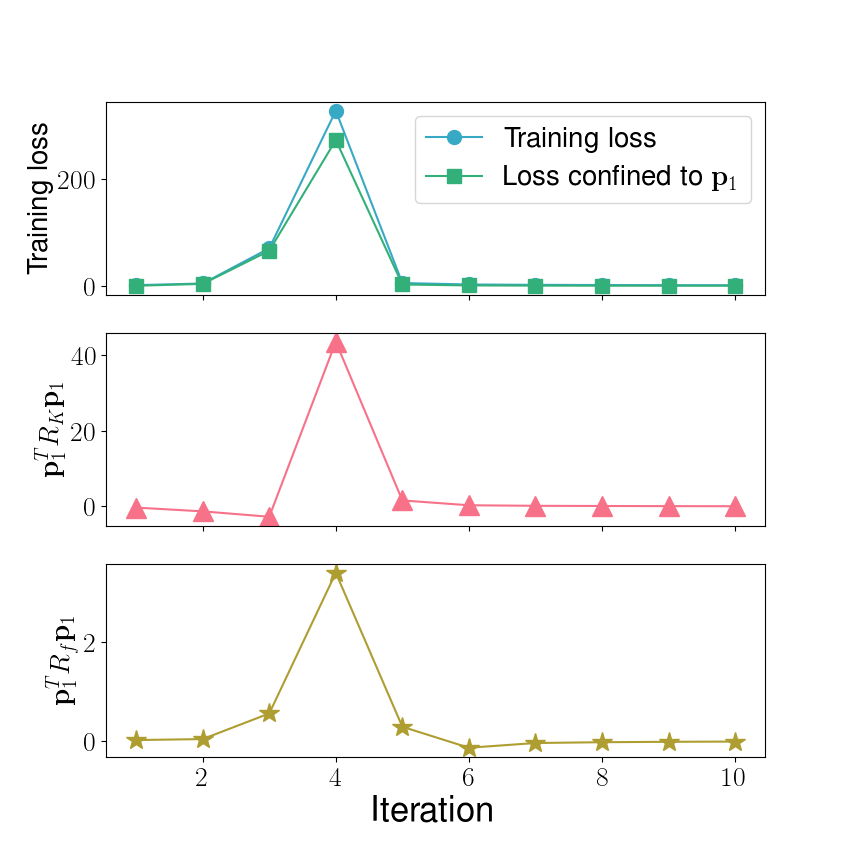
Refer to caption
(a) FC on CIFAR-2
Refer to caption
(b) CNN on CIFAR-2
Refer to caption
(c) FC on SVHN-2
Refer to caption
(d) CNN on SVHN-2
Figure 6: Training dynamics confined to the top eigenspace of the tangent kernel for NQMs.
Refer to caption
(a) FC on CIFAR-2
Refer to caption
(b) CNN on CIFAR-2
Refer to caption
(c) FC on SVHN-2
Refer to caption
(d) CNN on SVHN-2
Figure 7: Training dynamics confined to the top eigenspace of the tangent kernel for wide neural networks.

N.4 Training dynamics of general quadratic models and neural networks.

As discussed at the end of Section 3, a more general quadratic model can exhibit the catapult phase phenomenon. Specifically, we consider a general quadratic model:

g(𝐰;𝒙)=𝐰Tϕ(𝒙)+12γ𝐰TΣ(𝒙)𝐰.𝑔𝐰𝒙superscript𝐰𝑇italic-ϕ𝒙12𝛾superscript𝐰𝑇Σ𝒙𝐰\displaystyle g({\mathbf{w}};{\boldsymbol{x}})={\mathbf{w}}^{T}\phi({\boldsymbol{x}})+\frac{1}{2}\gamma{\mathbf{w}}^{T}\Sigma({\boldsymbol{x}}){\mathbf{w}}.

We will train the general quadratic model with different learning rates, and different γ𝛾\gamma respectively, to see how the catapult phase phenomenon depends on these two factors. For comparison, we also implement the experiments for neural networks. See the experiment setting in the following:

General quadratic models.

We set the dimension of the input d=100𝑑100d=100. We let the feature vector ϕ(𝒙)=𝒙/𝒙italic-ϕ𝒙𝒙norm𝒙\phi({\boldsymbol{x}})={\boldsymbol{x}}/\|{\boldsymbol{x}}\| where xi𝒩(0,1)similar-tosubscript𝑥𝑖𝒩01x_{i}\sim\mathcal{N}(0,1) i.i.d. for each i[d]𝑖delimited-[]𝑑i\in[d]. We let ΣΣ\Sigma be a diagonal matrix with Σi,i{1,1}subscriptΣ𝑖𝑖11\Sigma_{i,i}\in\{-1,1\} randomly and independently. The weight parameters 𝐰𝐰{\mathbf{w}} are initialized by 𝒩(0,Id)𝒩0subscript𝐼𝑑\mathcal{N}(0,I_{d}). Unless stated otherwise, γ=103𝛾superscript103\gamma=10^{-3}, and the learning rate is set to be 2.82.82.8.

Neural networks.

We train a two-layer fully-connected neural networks with ReLU activation function on 202020 data points of CIFAR-2. Unless stated otherwise, the network width is 104superscript10410^{4}, and the learning rate is set to be 2.82.82.8.

See the results in Figure 8.

(A) (B)
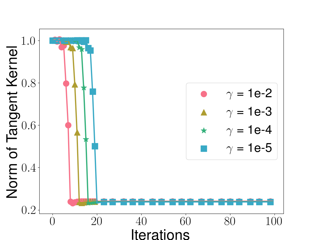
Refer to caption
Refer to caption
Refer to caption
Refer to caption
Refer to caption
(a) Loss (log scaled) vs. γ𝛾\gamma/width
Refer to caption
(b) Tangent kernel norm vs. γ𝛾\gamma/width
Refer to caption
(c) Loss vs. learning rate
Refer to caption
(d) Tangent kernel norm vs. learning rate
Figure 8: General quadratic models have similar training dynamics with neural networks when trained with super-critical learning rates. Panel (A): experiments on general quadratic models. Smaller γ𝛾\gamma or larger learning rates lead to larger training loss at the peak. Larger learning rates make tangent kernel decrease more. Panel (B): experiments on two-layer neural networks. Larger width (corresponding to smaller γ𝛾\gamma) and larger learning rates have similar effect on the training loss at the peak and decrease of tangent kernel norm with quadratic models. Note that width or γ𝛾\gamma seems to have no effect on the tangent kernel norm at convergence.

N.5 Test performance of f𝑓f, flinsubscript𝑓linf_{{{\mathrm{lin}}}} and fquadsubscript𝑓quadf_{{\mathrm{quad}}}, i.e., Figure 2(b) and Figure 4

For the architectures of two-layer fully connected neural network and two-layer convolutional neural network, we set the width to be 5,00050005,000 and 1,00010001,000 respectively. Specific to Figure 2(b), we use the architecture of a two-layer fully connected neural network.

Due to the large number of parameters in NQMs, we choose a small subset of all the datasets. We use the first class (airplanes) and third class (birds) of CIFAR-10, which we call CIFAR-2, and select 256256256 data points out of it as the training set. We use the number 00 and 222 of SVHN, and select 256256256 data points as the training set. We select 128128128, 256256256, 128128128 data points out of MNIST, FSDD and AG NEWS dataset respectively as the training sets. The size of testing set is 2,00020002,000 for all. When implementing SGD, we choose batch size to be 323232.

For each setting, we report the average result of 5 independent runs.

N.6 Test performance of f𝑓f, flinsubscript𝑓linf_{{{\mathrm{lin}}}} and fquadsubscript𝑓quadf_{{\mathrm{quad}}} in terms of accuracy

In this section, we report the best test accuracy for f𝑓f, flinsubscript𝑓linf_{{{\mathrm{lin}}}} and fquadsubscript𝑓quadf_{{\mathrm{quad}}} corresponding to the best test loss in Figure 4. We use the same setting as in Appendix N.5.
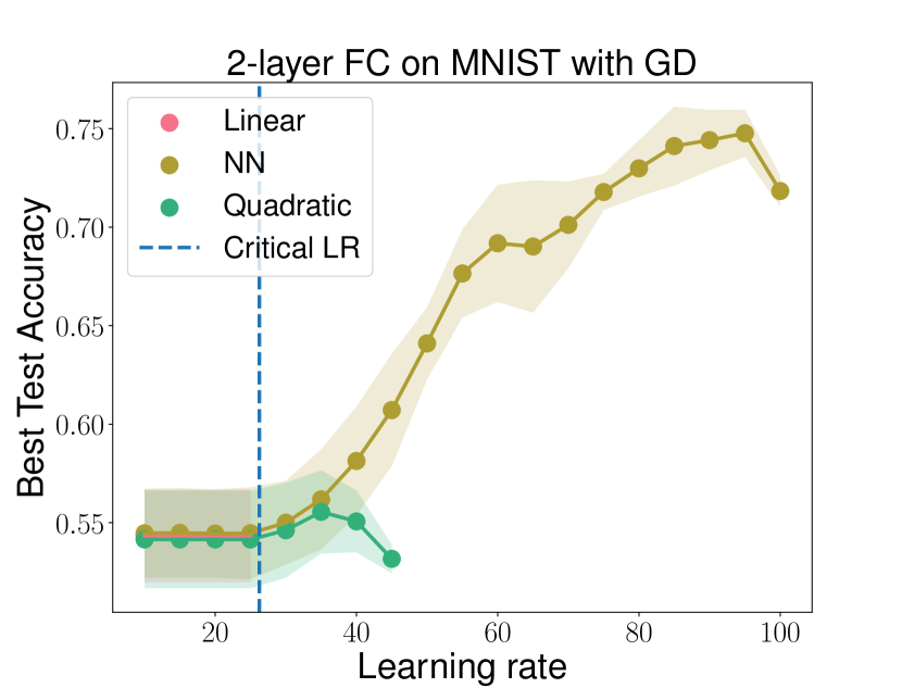
Refer to caption
Refer to caption
Figure 9: Best test accuracy plotted against different learning rates for fquadsubscript𝑓quadf_{{\mathrm{quad}}}, f𝑓f, and flinsubscript𝑓linf_{{{\mathrm{lin}}}}. Left panel: 2-layer FC on MNIST trained with GD. Right panel: 2-layer FC on AG NEWS trained with GD.
Refer to caption
Refer to caption
Figure 10: Best test accuracy plotted against different learning rates for fquadsubscript𝑓quadf_{{\mathrm{quad}}}, f𝑓f, and flinsubscript𝑓linf_{{{\mathrm{lin}}}}. Left panel: 2-layer FC on CIFAR-2 trained with SGD. Right panel: 2-layer CNN on SVHN trained with GD.
Refer to caption
Refer to caption
Figure 11: Best test accuracy plotted against different learning rates for fquadsubscript𝑓quadf_{{\mathrm{quad}}}, f𝑓f, and flinsubscript𝑓linf_{{{\mathrm{lin}}}}. Left panel: 2-layer FC on FSDD trained with GD. Right panel: 2-layer CNN on CIFAR-2 trained with GD.

N.7 Test performance of f𝑓f, flinsubscript𝑓linf_{{{\mathrm{lin}}}} and fquadsubscript𝑓quadf_{{\mathrm{quad}}} with architecture of 3-layer FC

In this section, we extend our results for shallow neural networks discussed in Section 4 to 3-layer fully connected neural networks. In the same way, we compare the test performance of three models, f𝑓f, flinsubscript𝑓linf_{{{\mathrm{lin}}}} and fquadsubscript𝑓quadf_{{\mathrm{quad}}} upon varying learning rate. We observe the same phenomenon for 3-layer ReLU activated FC with shallow neural networks. See Figure 12 and 13.

We use the first class (airplanes) and third class (birds) of CIFAR-10, which we call CIFAR-2, and select 100100100 data points out of it as the training set. We use the number 00 and 222 of SVHN, and select 100100100 data points as the training set. We select 100100100 data points out of AG NEWS dataset as the training set. For the speech data set FSDD, we select 100100100 data points in class 111 and 333 as the training set. The size of testing set is 500500500 for all.

For each setting, we report the average result of 5 independent runs.
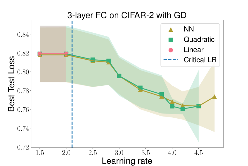
Refer to caption
Refer to caption
Figure 12: Best test accuracy plotted against different learning rates for fquadsubscript𝑓quadf_{{\mathrm{quad}}}, f𝑓f, and flinsubscript𝑓linf_{{{\mathrm{lin}}}}. Left panel: 3-layer FC on CIFAR-2 trained with GD. Right panel: 3-layer FC on SVHN-2 trained with GD.
Refer to caption
Refer to caption
Figure 13: Best test accuracy plotted against different learning rates for fquadsubscript𝑓quadf_{{\mathrm{quad}}}, f𝑓f, and flinsubscript𝑓linf_{{{\mathrm{lin}}}}. Left panel: 3-layer FC on FSDD-2 trained with GD. Right panel: 3-layer FC on AG NEWS trained with GD.

N.8 Test performance with Tanh and Swish activation functions

We replace ReLU by Tanh and Swish activation functions to train the models with the same setting as Figure 4. We observe the same phenomenon as we describe in Section 4.
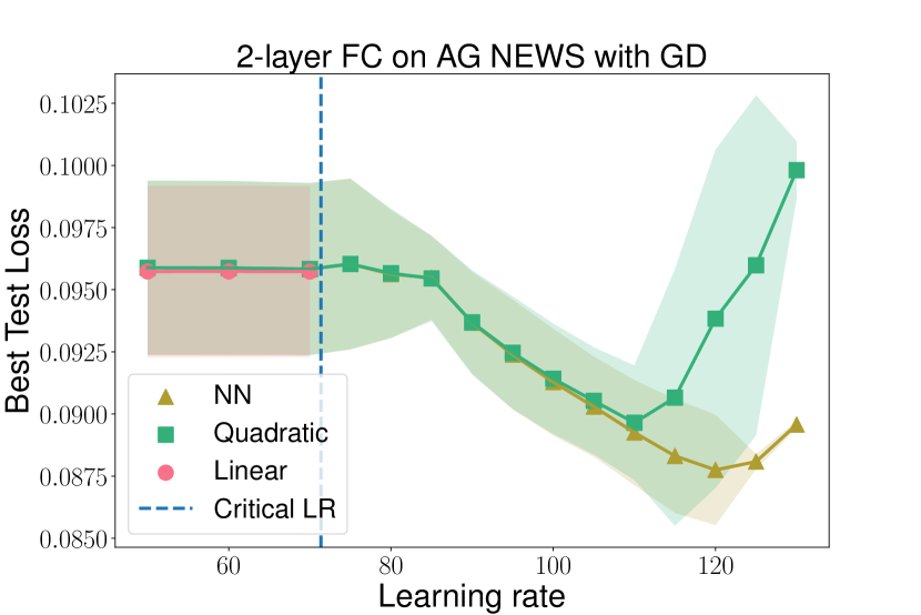
Refer to caption
(a) Swish activation function
Refer to caption
(b) Tanh activation function
Figure 14: Best test loss plotted against different learning rates for fquadsubscript𝑓quadf_{{\mathrm{quad}}}, f𝑓f, and flinsubscript𝑓linf_{{{\mathrm{lin}}}}. We choose 2-layer FC as the architecture and train the models on AG NEWS with GD.
Refer to caption
(a) Swish activation function
Refer to caption
(b) Tanh activation function
Figure 15: Best test loss plotted against different learning rates for fquadsubscript𝑓quadf_{{\mathrm{quad}}}, f𝑓f, and flinsubscript𝑓linf_{{{\mathrm{lin}}}}. We choose 2-layer FC as the architecture and train the models on FSDD with GD.
Refer to caption
(a) Swish activation function
Refer to caption
(b) Tanh activation function
Figure 16: Best test loss plotted against different learning rates for fquadsubscript𝑓quadf_{{\mathrm{quad}}}, f𝑓f, and flinsubscript𝑓linf_{{{\mathrm{lin}}}}. We choose 2-layer CNN as the architecture and train the models on CIFAR-2 with GD.
Refer to caption
(a) Swish activation function
Refer to caption
(b) Tanh activation function
Figure 17: Best test loss plotted against different learning rates for fquadsubscript𝑓quadf_{{\mathrm{quad}}}, f𝑓f, and flinsubscript𝑓linf_{{{\mathrm{lin}}}}. We choose 2-layer CNN as the architecture and train the models on SVHN with GD.