Semi-Parametric Inducing Point Networks and Neural Processes

Abstract

We introduce semi-parametric inducing point networks (SPIN), a general-purpose architecture that can query the training set at inference time in a compute-efficient manner. Semi-parametric architectures are typically more compact than parametric models, but their computational complexity is often quadratic. In contrast, SPIN attains linear complexity via a cross-attention mechanism between datapoints inspired by inducing point methods. Querying large training sets can be particularly useful in meta-learning, as it unlocks additional training signal, but often exceeds the scaling limits of existing models. We use SPIN as the basis of the Inducing Point Neural Process, a probabilistic model which supports large contexts in meta-learning and achieves high accuracy where existing models fail. In our experiments, SPIN reduces memory requirements, improves accuracy across a range of meta-learning tasks, and improves state-of-the-art performance on an important practical problem, genotype imputation.

1 Introduction

Recent advances in deep learning have been driven by large-scale parametric models (Krizhevsky et al., 2012; Peters et al., 2018; Devlin et al., 2019; Brown et al., 2020; Ramesh et al., 2022). Modern parametric models rely on large numbers of weights to capture the signal contained in the training set and to facilitate generalization (Frankle & Carbin, 2018; Kaplan et al., 2020); as a result, they require non-trivial computational resources (Hoffmann et al., 2022), have limited interpretability (Belinkov, 2022), and impose a significant carbon footprint (Bender et al., 2021).

This paper focuses on an alternative semi-parametric approach, in which we have access to the training set $\mathcal{D}_{\mathrm{train}}=\{\mathbf{x}^{(i)},\mathbf{y}^{(i)}\}_{i=1}^{n}$ at inference time and learn a parametric mapping $\mathbf{y}=f_{\theta}(\mathbf{x}\mid\mathcal{D}_{\mathrm{train}})$ conditioned on this dataset. Semi-parametric models can query the training set $\mathcal{D}_{\mathrm{train}}$ and can therefore express rich and interpretable mappings with a compact $f_{\theta}$. Examples of the semi-parametric framework include retrieval-augmented language models (Grave et al., 2016; Guu et al., 2020; Rae et al., 2021) and non-parametric transformers (Wiseman & Stratos, 2019; Kossen et al., 2021). However, existing approaches are often specialized to specific tasks (e.g., language modeling (Grave et al., 2016; Guu et al., 2020; Rae et al., 2021) or sequence generation (Graves et al., 2014)), and their computation scales superlinearly in the size of the training set (Kossen et al., 2021).

Here, we introduce semi-parametric inducing point networks (SPIN), a general-purpose architecture whose computational complexity at training time scales linearly in the size of the training set $\mathcal{D}_{\mathrm{train}}$ and in the dimensionality of $\mathbf{x}$ and that is constant in $\mathcal{D}_{\mathrm{train}}$ at inference time. Our architecture is inspired by inducing point approximations (Snelson & Ghahramani, 2005; Titsias, 2009; Wilson & Nickisch, 2015; Evans & Nair, 2018; Lee et al., 2018) and relies on a cross-attention mechanism between datapoints (Kossen et al., 2021). An important application of SPIN is in meta-learning, where conditioning on large training sets provides the model additional signal and improves accuracy, but poses challenges for methods that scale superlinearly with $\mathcal{D}_{\mathrm{train}}$. We use SPIN as the basis of the Inducing Point Neural Process (IPNP), a scalable probabilistic model that supports accurate meta-learning with large context sizes that cause existing methods to fail. We evaluate SPIN and IPNP on a range of supervised and meta-learning benchmarks and demonstrate the efficacy of SPIN on a real-world task in genomics—genotype imputation (Li et al., 2009). In meta-learning experiments, IPNP supports querying larger training sets, which yields high accuracy in settings where existing methods run out of memory. In the genomics setting, SPIN outperforms highly engineered state-of-the-art software packages widely used within commercial genomics pipelines (Browning et al., 2018b), indicating that our technique has the potential to impact real-world systems.

Contributions

In summary, we introduce SPIN, a semi-parametric neural architecture inspired by inducing point methods that is the first to achieve the following characteristics:

1. Linear time and space complexity in the size and the dimension of the data during training.

2. The ability to learn a compact encoding of the training set for downstream applications. As a result, at inference time, computational complexity does not depend on training set size.

We use SPIN as the basis of the IPNP, a probabilistic model that enables performing meta-learning with context sizes that are larger than what existing methods support and that achieves high accuracy on important real-world tasks such as genotype imputation.

2 Background

Parametric and Semi-Parametric Machine Learning

Most supervised methods in deep learning are parametric. Formally, given a training set $\mathcal{D}_{\mathrm{train}}=\{\mathbf{x}^{(i)},\mathbf{y}^{(i)}\}_{i=1}^{n}$ with features $\mathbf{x}\in\mathcal{X}$ and labels $\mathbf{y}\in\mathcal{Y}$, we seek to learn a fixed number of parameters $\theta\in\Theta$ of a mapping $\mathbf{y}=f_{\theta}(\mathbf{x})$ using supervised learning. In contrast, non-parametric approaches learn a mapping $\mathbf{y}=f_{\theta}(\mathbf{x}\mid\mathcal{D}_{\mathrm{train}})$ that can query the training set $\mathcal{D}_{\mathrm{train}}$ at inference time; when the mapping $f_{\theta}$ has parameters, the approach is called semi-parametric. Many deep learning algorithms—including memory-augmented architectures (Graves et al., 2014; Santoro et al., 2016), retrieval-based language models (Grave et al., 2016; Guu et al., 2020; Rae et al., 2021), and non-parametric transformers (Kossen et al., 2021)—are instances of this approach, but they are often specialized to specific tasks, and their computation scales superlinearly in $n$. This paper develops scalable and domain-agnostic semi-parametric methods.

Meta-Learning and Neural Processes

An important application of semi-parametric methods is in meta-learning, where we train a model to achieve high performance on new tasks using only a small amount of data from these tasks. Formally, consider a collection of $D$ datasets (or a meta-dataset) $\{\mathcal{D}^{(d)}\}_{d=1}^{D}$, each defining a task. Each $\mathcal{D}^{(d)}=(\mathcal{D}^{(d)}_{c},\mathcal{D}^{(d)}_{t})$ contains a set of context points $\mathcal{D}^{(d)}_{c}=\{\mathbf{x}^{(di)}_{c},\mathbf{y}^{(di)}_{c}\}_{i=1}^{m}$ and target points $\mathcal{D}^{(d)}_{t}=\{\mathbf{x}^{(di)}_{t},\mathbf{y}^{(di)}_{t}\}_{i=1}^{n}$. Meta-learning seeks to produce a model $f(\mathbf{x};\mathcal{D}_{c})$ that outputs accurate predictions for $\mathbf{y}$ on $\mathcal{D}_{t}$ and on pairs $(\mathcal{D}_{c},\mathcal{D}_{t})$ not seen at training time. Neural Process (NP) architectures perform uncertainty aware meta-learning by mapping context sets to representations $\mathbf{r}_{c}(\mathcal{D}_{c}),$ which can be combined with target inputs to provide a distribution on target labels $\mathbf{y}_{t}\sim p(\mathbf{y}|\mathbf{x}_{t},\mathbf{r}_{c}(\mathcal{D}_{c}))$, where $p$ is a probabilistic model. Recent successes in NPs have been driven by attention-based architectures (Kim et al., 2018; Nguyen & Grover, 2022), whose complexity scales super-linearly with context size $\mathcal{D}_{c}$—our method yields linear complexity. In concurrent work, Feng et al. (2023) propose a linear time method, using cross attention to reduce the size of context datasets.

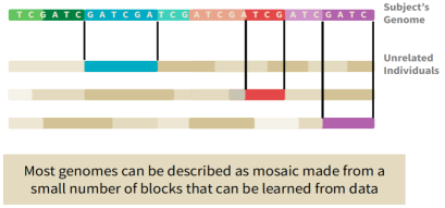
Figure 1: Genotype recombination

A Motivating Application: Genotype Imputation

A specific motivating example for developing efficient semi-parametric methods is the problem of genotype imputation. Consider the problem of determining the genomic sequence $\mathbf{y}\in\{\mathrm{A},\mathrm{T},\mathrm{C},\mathrm{G}\}^{k}$ of an individual; rather than directly measuring $\mathbf{y}$, it is common to use an inexpensive microarray device to measure a small subset of genomic positions $\mathbf{x}\in\{\mathrm{A},\mathrm{T},\mathrm{C},\mathrm{G}\}^{p}$, where $p\ll k$. Genotype imputation is the task of determining $\mathbf{y}$ from $\mathbf{x}$ via statistical methods and a dataset $\mathcal{D}_{\mathrm{train}}=\{\mathbf{x}^{(i)},\mathbf{y}^{(i)}\}_{i=1}^{n}$ of fully-sequenced individuals (Li et al., 2009). Imputation is part of most standard genome analysis workflows. It is also a natural candidate for semi-parametric approaches (Li & Stephens, 2003): a query genome $\mathbf{y}$ can normally be represented as a combination of sequences $\mathbf{y}^{(i)}$ from $\mathcal{D}_{\mathrm{train}}$ because of the biological principle of recombination (Kendrew, 2009), as shown in Figure 1. Additionally, the problem is a poor fit for parametric models: $k$ can be as high as $10^{9}$ and there is little correlation across non-proximal parts of $\mathbf{y}$. Thus, we need an unwieldy number of parametric models (one per subset of $\mathbf{y}$), whereas a single semi-parametric model can run imputation across the genome.

Attention Mechanisms

Our approach for designing semi-parametric models relies on modern attention mechanisms (Vaswani et al., 2017), specifically dot-product attention $\mathrm{Att}(\mathbf{Q},\mathbf{K},\mathbf{V})$, which combines a query matrix $\mathbf{Q}\in\mathbb{R}^{d_{q}\times e_{q}}$ with key and value matrices $\mathbf{K}\in\mathbb{R}^{d_{v}\times e_{q}}$, $\mathbf{V}\in\mathbb{R}^{d_{v}\times e_{v}}$ as

$$\mathrm{Att}(\mathbf{Q},\mathbf{K},\mathbf{V})=\mathrm{softmax}(\mathbf{Q}\mathbf{K}^{\top}/\sqrt{e_{q}})\mathbf{V}\vspace{-5pt}$$

To attend to different aspects of the keys and values, multi-head attention (MHA) extends this mechanism via $e_{h}$ attention heads:

$$\mathrm{MHA}(\mathbf{Q},\mathbf{K},\mathbf{V})=\textrm{concat}(\mathbf{O}_{1},...\mathbf{O}_{e_{h}})\mathbf{W}^{O} \mathbf{O}_{j}=\mathrm{Att}(\mathbf{Q}\mathbf{W}^{Q}_{j},\mathbf{K}\mathbf{W}^{K}_{j},\mathbf{V}\mathbf{W}^{V}_{j})$$

Each attention head projects $\mathbf{Q},\mathbf{K},\mathbf{V}$ into a lower-dimensional space using learnable projection matrices $\mathbf{W}_{j}^{Q},\mathbf{W}_{j}^{K}\in\mathbb{R}^{e_{q}\times e_{qh}}$, $\mathbf{W}_{j}^{V}\in\mathbb{R}^{e_{v},e_{vh}}$ and mixes the outputs of the heads using $\mathbf{W}^{O}\in\mathbb{R}^{e_{h}e_{vh}\times e_{o}}$. As is commonly done, we assume that $e_{vh}=e_{v}/e_{h}$, $e_{qh}=e_{q}/e_{h}$, and $e_{o}=e_{q}$. Given two matrices $\mathbf{X},\mathbf{H}\in\mathbb{R}^{d\times e}$, a multi-head attention block (MAB) wraps MHA together with layer normalization and a fully connected layer:

$$\mathrm{MAB}(\mathbf{X},\mathbf{H})=\mathbf{O}+\textrm{FF}(\textrm{LayerNorm}(\mathbf{O})) \mathbf{O}=\mathbf{X}+\mathrm{MHA}(\textrm{LayerNorm}(\mathbf{X}),\mathbf{H},\mathbf{H})$$

Attention in semi-parametric models normally scales quadratically in the dataset size (Kossen et al., 2021); our work is inspired by efficient attention architectures (Lee et al., 2018; Jaegle et al., 2021b) and develops scalable semi-parametric models with linear computational complexity.

3 Semi-Parametric Inducing Point Networks

3.1 Semi-Parametric Learning Based on Neural Inducing Points

A key challenge posed by semi-parametric methods—one affecting both classical kernel methods (Hearst et al., 1998) as well as recent attention-based approaches (Kossen et al., 2021)—is the $O(n^{2})$ computational cost per gradient update at training time, due to pairwise comparisons between training set points . Our work introduces methods that reduce this cost to $O(hn)$—where $h\ll n$ is a hyper-parameter—without sacrificing performance.

Neural Inducing Points

Our approach is based on inducing points, a technique popular in approximate kernel methods (Wilson & Nickisch, 2015; Lee et al., 2018). A set of inducing points $\mathcal{H}=\{\mathbf{h}^{(j)}\}_{j=1}^{h}$ can be thought of as a “virtual” set of training instances that can replace the training set $\mathcal{D}_{\mathrm{train}}$. Intuitively, when $\mathcal{D}_{\mathrm{train}}$ is large, many datapoints are redundant—for example, groups of similar $\mathbf{x}^{(i)}$ can be replaced with a single inducing point $\mathbf{h}^{(j)}$ with little loss of information.

The key challenge in developing inducing point methods is finding a good set $\mathcal{H}$. While classical approaches rely on optimization techniques (Wilson & Nickisch, 2015), we use an attention mechanism to produce $\mathcal{H}$. Each inducing point $\mathbf{h}^{(j)}\in\mathcal{H}$ attends over the training set $\mathcal{D}_{\mathrm{train}}$ to select its relevant “neighbors” and updates itself based on them. We implement attention between $\mathcal{H}$ and $\mathcal{D}_{\mathrm{train}}$ in $O(hn)$ time.

Dataset Encoding

Note that once we have a good set of inducing points $\mathcal{H}$, it becomes possible to discard $\mathcal{D}_{\mathrm{train}}$ and use $\mathcal{H}$ instead for all future predictions. The parametric part of the model makes predictions based on $\mathcal{H}$ only. This feature is an important capability of our architecture; computational complexity is now independent of $\mathcal{D}$ and we envision this feature being useful in applications where sharing $\mathcal{D}_{\mathrm{train}}$ is not possible (e.g., for computational or privacy reasons).

3.2 Semi-Parametric Inducing Point Networks

Next, we describe semi-parametric inducing point networks (SPIN), a domain-agnostic architecture with linear-time complexity.

Notation and Data Embedding

The SPIN model relies on a training set $\mathcal{D}_{\mathrm{train}}=\{\mathbf{x}^{(i)},\mathbf{y}^{(i)}\}_{i=1}^{n}$ with input features $\mathbf{x}^{(i)}\in\mathcal{X}$ and labels $\mathbf{y}^{(i)}\in\mathcal{Y}$ where $\mathcal{X},\mathcal{Y}\in\mathcal{V}$, which is the input and output vocabulary . We embed each dimension (each attribute) of $\mathbf{x}$ and $\mathbf{y}$ into an $e$-dimensional embedding and represent $\mathcal{D}_{\mathrm{train}}$ as a tensor of embeddings $\mathbf{D}=\text{Embed}(\mathcal{D}_{\text{train}})$, $\mathbf{D}\in\mathbb{R}^{n\times d\times e}$, where $d=p+k$ is obtained from concatenating the sequence of embeddings for each $\mathbf{x}^{(i)}$ and $\mathbf{y}^{(i)}$.

The set $\mathcal{D}_{\mathrm{train}}$ is used to learn inducing points $\mathcal{H}=\{\mathbf{h}^{(j)}\}_{j=1}^{h}$; similarly, we represent $\mathcal{H}$ via a tensor $\mathbf{H}\in\mathbb{R}^{h\times f\times e}$ of $h\leq n$ inducing points, each being a sequence of $f\leq d$ embeddings of size $e$.

To make predictions and measure loss on a set of $b$ examples $\mathcal{D}_{\mathrm{query}}=\{\mathbf{x}^{(i)},\mathbf{y}^{(i)}\}_{i=1}^{b}$, we use the same embedding procedure to obtain a tensor of input embeddings $\mathbf{X}_{\mathrm{query}}\in\mathbb{R}^{b\times d\times e}$ by embedding $\{\mathbf{x}^{(i)},{\bf 0}\}_{i=1}^{b}$, in which the labels have been masked with zeros. We also use a tensor $\mathbf{Y}_{\mathrm{gold}}\in\mathbb{R}^{b\times d}$ to store the ground truth labels and inputs (the objective function we use requires the model to make predictions on masked input elements as well, see below for details).

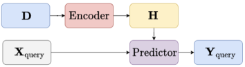
Figure 2: SPIN Model Structure

High-Level Model Structure

Figure 2 presents an overview of SPIN. At a high level, there are two components: (1) an $\mathrm{Encoder}$ module, which takes as input $\mathcal{D}_{\mathrm{train}}$ and returns a tensor of inducing points $\mathbf{H}$; and (2) a $\mathrm{Predictor}$ module, which is a fully parametric model that outputs logits $\mathbf{Y}_{\mathrm{query}}$ from $\mathbf{H}$ and $\mathbf{X}_{\mathrm{query}}$.

$$\mathbf{D}=\text{Embed}(\mathcal{D}_{\mathrm{train}}) \mathbf{H}=\mathrm{Encoder}(\mathbf{D}) \mathbf{Y}_{\mathrm{query}}=\mathrm{Predictor}(\mathbf{X}_{\mathrm{query}},\mathbf{H})$$

The encoder consists of a sequence of layers, each of which takes as input $\mathbf{D}\in\mathbb{R}^{n\times d\times e}$ and two tensors $\mathbf{H}_{A}\in\mathbb{R}^{n\times f\times e}$ and $\mathbf{H}_{D}\in\mathbb{R}^{h\times f\times e}$ and output updated versions of $\mathbf{H}_{A},\mathbf{H}_{D}$ for the next layer. Each layer consists of a sequence of up to three cross-attention layers described below. The final output $\mathbf{H}$ of the encoder is the $\mathbf{H}_{D}$ produced by the last layer.

3.2.1 Architecture of the Encoder and Predictor

Each layer of the encoder consists of three sublayers denoted as $\mathrm{XABA},\mathrm{XABD},\mathrm{ABLA}$. An encoder layer takes as input $\mathbf{H}_{A},\mathbf{H}_{D}$ and feeds its outputs $\mathbf{H}_{A}^{\prime},\mathbf{H}_{D}^{\prime}$ (defined below) into the next layer. The initial inputs $\mathbf{H}_{A},\mathbf{H}_{D}$ of the first encoder layer are randomly initialized learnable parameters.

$$\mathbf{H}_{A}^{\prime}=\mathrm{XABA}(\mathbf{H}_{A},\mathbf{D}) \mathbf{H}_{D}^{\prime}=\mathrm{XABD}(\mathbf{H}_{D},\mathbf{H}_{A}^{\prime}) \mathbf{H}_{A}=\mathrm{ABLA}(\mathbf{H}_{A}^{\prime})$$

Cross-Attention Between Attributes ($\mathrm{XABA}$)

An $\mathrm{XABA}$ layer captures the dependencies among attributes via cross-attention between the sequence of latent encodings in $\mathbf{H}$ and the sequence of datapoint features in $\mathbf{D}$.

$$\mathrm{XABA}(\mathbf{H}_{A},\mathbf{D})=\mathrm{MAB}(\mathbf{H}_{A},\mathbf{D})$$

This updates the features of each datapoint in $\mathbf{H}_{A}$ to be a combination of the features of the corresponding datapoints in $\mathbf{D}$. In effect, this reduces the dimensionality of the datapoints (from $n\times d\times e$ to $n\times f\times e)$. The time complexity of this layer is $O(ndfe)$, where $f$ is the dimensionality of the reduced tensor.

Cross-Attention Between Datapoints ($\mathrm{XABD}$)

The $\mathrm{XABD}$ layer is the key module that takes into account the entire training set to generate inducing points.

First, it reshapes (“$\mathrm{unfold}$s”) its input tensors $\mathbf{H}_{A}^{\prime}\in\mathbb{R}^{n\times f\times e}$ and $\mathbf{H}_{D}\in\mathbb{R}^{h\times f\times e}$ into ones of dimensions $(1\times n\times fe)$ and $(1\times h\times fe)$ respectively. It then performs cross-attention between the two unfolded tensors. The output of cross-attention has dimension $(1\times h\times fe)$; it is reshaped (“$\mathrm{fold}$ed”) into an output tensor of size $(h\times f\times e)$.

$$\mathrm{XABD}(\mathbf{H}_{D},\mathbf{H}_{A}^{\prime})=\mathrm{fold}(\mathrm{MAB}(\mathrm{unfold}(\mathbf{H}_{D}),\mathrm{unfold}(\mathbf{H}_{A}^{\prime}))$$

This layer produces inducing points. Each inducing point in $\mathbf{H}_{D}$ attends to dimensionality-reduced datapoints in $\mathbf{H}_{A}^{\prime}$ and uses its selected datapoints to update its own representation. The computational complexity of this operation is $O(nhfe)$, which is linear in training set size $n$.

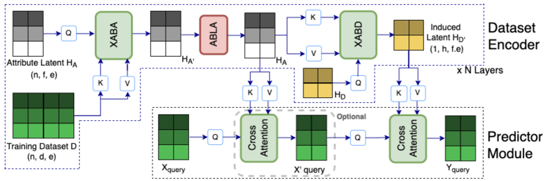
Figure 3: SPIN Architecture. Each layer of the encoder consists of sublayers XABA, ABLA and XABD, and the predictor consists of a cross attention layer. We omit feedforward layers for simplicity.

Self-Attention Between Latent Attributes ($\mathrm{ABLA}$)

The third type of layer further captures dependencies among attributes by computing regular self-attention across attributes:

$$\text{ABLA}(\mathbf{H}_{A}^{\prime})=\mathrm{MAB}(\mathbf{H}_{A}^{\prime},\mathbf{H}_{A}^{\prime})$$

This enables the inducing points to refine their internal representations. The dataset encoder consists of a sequence of the above layers, see Figure 3. The $\mathrm{ABLA}$ layers are optional based on validation performance. The input $\mathbf{H}_{D}$ to the first layer is part of the learned model parameters; the initial $\mathbf{H}_{A}$ is a linear projection of $\mathbf{D}$. The output of the encoder is the output $\mathbf{H}_{D}^{\prime}$ of the final layer.

Predictor Architecture

The predictor is a parametric model that maps an input tensor $\mathbf{X}_{\mathrm{query}}$ to an output tensor of logits $\mathbf{Y}_{\mathrm{query}}$. The predictor can use any parametric model. We propose an architecture based on a simple cross-attention operation followed by a linear projection to the vocabulary size, as shown in Figure 3:

$$\text{Predict}(\mathbf{X}_{\mathrm{query}},\mathbf{H})=\textrm{FF}(\mathrm{MAB}(\mathrm{unfold}(\mathbf{X}_{\mathrm{query}}),\mathrm{unfold}(\mathbf{H})))$$

3.3 Inducing Point Neural Processes

An important application of SPIN is in meta-learning, where conditioning on larger training sets provides more information to the model, and therefore has potential to improve predictive accuracy. However, existing methods scale superlinearly with $\mathcal{D}_{\mathrm{train}}$, and may not effectively leverage large contexts. We use SPIN as the basis of the Inducing Point Neural Process (IPNP), a scalable probabilistic model that supports fast and accurate meta-learning on large context sizes.

An IPNP defines a probabilistic model $p(\mathbf{y}|\mathbf{x},\mathbf{r}(\mathbf{x},\mathcal{D}_{c}))$ of a target variable $\mathbf{y}$ conditioned on an input $\mathbf{x}$ and a context dataset $\mathcal{D}_{c}.$ This context is represented via a fixed-dimensional context vector $r(\mathbf{x},\mathcal{D}_{c}),$ and we use the SPIN architecture to parameterize $\mathbf{r}$ as a function of $\mathcal{D}_{c}$. Specifically, we define $\mathbf{r}_{c}=\mathrm{Encoder}(\text{Embed}(\mathcal{D}_{c}))$, where $\mathrm{Encoder}$ is the SPIN encoder, producing a tensor of inducing points. Then, we compute $\mathbf{r}(\mathbf{x},\mathbf{r}_{c})=\mathrm{MAB}(\mathbf{x},\mathbf{r}_{c})$ via cross-attention. The model $p(\mathbf{y}|\mathbf{x},\mathbf{r})$ is a distribution with parameters $\phi(\mathbf{x},\mathbf{r})$, e.g., a Normal distribution with $\phi=(\mu,\Sigma)$ or a Bernoulli with $\phi\in[0,1]$. We parameterize the mapping $\phi(\mathbf{x},\mathbf{r})$ with a fully-connected neural network.

We further extend IPNPs to incorporate a latent variable $\mathbf{z}$ that is drawn from a Gaussian $p(\mathbf{z}|\mathcal{D}_{c})$ parameterized by $\phi_{\mathbf{z}}=m(\mathrm{Encoder}(\text{Embed}(\mathcal{D}_{c})))$, where $m$ represents mean pooling across datapoints. This latent variable can be thought of as capturing global uncertainty (Garnelo et al., 2018). This results in a distribution $p(\mathbf{y},\mathbf{z}|\mathbf{x},\mathcal{D}_{c})=p(\mathbf{y}|\mathbf{z},\mathbf{x},\mathcal{D}_{c})p(\mathbf{z}|\mathcal{D}_{c})$, where $p(\mathbf{y}|\mathbf{z},\mathbf{x},\mathcal{D}_{c})$ is parameterized by $\phi(\mathbf{z},\mathbf{x},\mathbf{r}_{c})$, with $\phi$ itself being a fully connected neural network. See Section A.6 for more detailed architectural breakdowns. Following terminology in the NP literature, we refer to our model as a conditional IPNP (CIPNP) when there is no latent variable $\mathbf{z}$ present.

3.4 Objective Function

SPIN

We train SPIN models using a supervised learning loss $\mathcal{L}^{\text{labels}}$ (e.g., $\ell_{2}$ loss for regression, cross-entropy for classification). We also randomly mask attributes and add an additional loss term $\mathcal{L}^{\text{attributes}}$ that asks the model to reconstruct the missing attributes, yielding the following objective:

$$\mathcal{L}^{\textrm{SPIN}}=(1-\lambda)\mathcal{L}^{\textrm{labels}}+\lambda\mathcal{L}^{\textrm{attributes}}$$

Following Kossen et al. (2021), we start with a weight $\lambda$ of 0.5 and anneal it to lean towards zero. We detail the loss terms and construction of mask matrices over labels and attrbutes in Section A.2. Following prior works (Devlin et al., 2019; Ghazvininejad et al., 2019; Kossen et al., 2021), we use random token level masking. Additionally, we propose chunk masking, similar to the span masking introduced in (Joshi et al., 2019), where a fraction $\rho$ of the samples selected have the mask matrix for labels $M^{(i)}=1$, and we show the effectiveness of chunk masking in Table 5.

IPNP

Following the NP literature, IPNPs are trained on a meta-dataset $\{\mathcal{D}^{(d)}\}_{d=1}^{D}$ of context and training points $\mathcal{D}^{(d)}=(\mathcal{D}^{(d)}_{c},\mathcal{D}^{(d)}_{t})$ to maximize the log likelihood of the target labels under the learned parametric distribution $\mathcal{L}^{\mathrm{IPNP}}=-\frac{1}{|D|}\sum_{d=1}^{D}\sum_{i=1}^{n}\log p(\mathbf{y}_{t}^{(di)}\mid\mathcal{D}_{c}^{(d)},\mathbf{x}_{t}^{(di)}).$ For latent variable NPs, the objective is a variational lower bound; see Section A.6 for more details.

4 Experiments

Semi-parametric models—including Neural Processes for meta-learning—benefit from large context sets $\mathcal{D}_{c}$, as they provide additional training signal. However, existing methods scale superlinearly with $\mathcal{D}_{c}$ and quickly run out of memory. In our experiments section, we show that SPIN and IPNP outperform state-of-the-art models by scaling to large $\mathcal{D}_{c}$ that existing methods do not support.

4.1 UCI Datasets

We present experimental results for 10 standard UCI benchmarks, namely Yacht, Concrete, Boston-Housing, Protein (regression datasets), Kick, Income, Breast Cancer, Forrest Cover, Poker-Hand and Higgs Boson (classification datasets). We compare SPIN with Transformer baselines such as NPT (Kossen et al., 2021) and Set Transformers (Set-TF) (Lee et al., 2018). We also evaluate against Gradient Boosting (GBT) Friedman (2001), Multi Layer Perceptron (MLP) (Hinton, 1989; Glorot & Bengio, 2010), and K-Nearest Neighbours (KNN) (Altman, 1992).

Table 1: Performance Summary on UCI Datasets

	Traditional ML			Transformer
	GBT	MLP	KNN	NPT	Set-TF	SPIN
Ranking $\downarrow$	3.00$\pm$1.76	4.10$\pm$1.37	5.44$\pm$1.01	2.30$\pm$1.25	3.63$\pm$0.92	2.10$\pm$0.88
GPU Mem $\downarrow$	-	-	-	1.0x	1.39$\pm$0.67x	0.46$\pm$0.21x

Table 2: Effect of context size on the Poker Hand dataset

		Context Size
Approach		4096	10K	15K	30K
NPT	Acc$\uparrow$	80.11	OOM	-	-
	Mem$\downarrow$	9.82	OOM	-	-
SPIN	Acc$\uparrow$	82.98	95.99	96.06	99.43
	Mem$\downarrow$	1.73	3.88	5.68	10.98
	GBT	MLP		KNN
Acc$\uparrow$	71.88 $\pm$5.91	66.09 $\pm$9.88		54.75 $\pm$0.03

Following Kossen et al. (2021), we measure the average ranking of the methods and standardize across all UCI tasks. To show the memory efficiency of our approach, we also report GPU memory usage peaks and as a fraction of GPU memory used by NPT for different splits of the test dataset in Table 1.

Results

SPIN achieves the best
average ranking on 10 UCI datasets and uses half the GPU memory

compared to NPT. We provide detailed results on each of the datasets and hyperparameter details in Section A.4. Importantly, SPIN achieves high performance by supporting larger context sets—we illustrate this in Table 2, where we compare SPIN and NPT on the Poker Hand dataset (70/20/10 split) using various context sizes. SPIN and NPT achieve 80-82% accuracy with small contexts, but the performance of SPIN approaches 99% as context size is increased, whereas NPT quickly runs out of GPU memory and fails to reach comparable performance.

4.2 Neural Processes for Meta-Learning

Experimental Setup

Following previous work (Kim et al., 2018; Nguyen & Grover, 2022), we perform a Gaussian process meta-learning experiment, for which we create a collection of datasets $(\mathcal{D}^{(d)})_{d=1}^{D}$, where each $\mathcal{D}^{(d)}$ contains random points $(\mathbf{x}^{(di)})_{i=1}^{m}$, where $\mathbf{x}^{(di)}\in\mathbb{R}$, and target points $\mathbf{y}^{(di)}=f^{(d)}(\mathbf{x}^{(di)})$ obtained from a function $f^{(d)}$ sampled from a Gaussian Process. At each meta-training step, we sample $B=16$ functions $\{f^{(b)}\}^{B}_{b=1}.$ For each $f^{(b)},$ we sample $m\sim\mathcal{U}[\texttt{min\_ctx},~{}\texttt{max\_ctx}]$ context points and $n\sim\mathcal{U}[\texttt{min\_tgt},~{}\texttt{max\_tgt}]$ target points. The range for $n$ is fixed across all experiments at $[4,64].$ The range for $m$ is varied from $[64,128],[128,256],[256,512],[512,1024],[1024,2048].$ We train several different NP models for 100,000 steps and evaluate their log-likelihood on 3,000 hold out batches, with $B,m,n$ taking the same values as at training time. We evaluate conditional (CIPNP) and latent variable (IPNP) variations of our model (using $h=\frac{1}{2}\cdot\texttt{min\_ctx}$ inducing points) and compare them to other attention-based NPs: Conditional ANPs (CANP) (Kim et al., 2018), Bootstrap ANPs (BANP) (Lee et al., 2020), and latent variable ANPs (ANP) (Kim et al., 2018).

Results

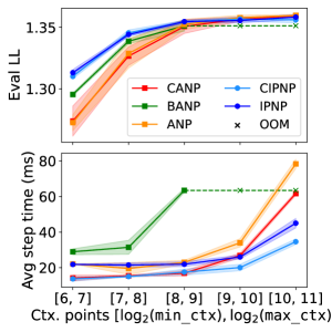
Figure 4: Inducing Point NPs outperform NP baselines and train much faster. Plots display mean $\pm$ std. deviation from 5 runs with different random seeds.

The IPNP models attain higher performance than all baselines at most context sizes (Figure 4).
Interestingly, IPNPs generalize better—recall that
IPNPs are more compact models with fewer parameters, hence are less likely to overfit. We also found that increased context size led to improved performance for all models; however, baseline NPs required excessive resources, and BANPs ran out of memory entirely. In contrast, IPNPs scaled to large context sizes using up to 50% less resources.

4.3 Genotype Imputation

Genotype imputation is the task of inferring the
sequence $\mathbf{y}$ of an entire genome via statistical methods from a small subset of positions $\mathbf{x}$—usually obtained from an inexpensive DNA microarray device (Li et al., 2009)—and a dataset $\mathcal{D}_{\mathrm{train}}=\{\mathbf{x}^{(i)},\mathbf{y}^{(i)}\}_{i=1}^{n}$ of fully-sequenced individuals (Li et al., 2009). Imputation is part of most standard workflows in genomics (Lou et al., 2021) and involves mature imputation software (Browning et al., 2018a; Rubinacci et al., 2020) that benefits from over a decade of engineering (Li & Stephens, 2003). These systems are fully non-parametric and match genomes in $\mathcal{D}_{\mathrm{train}}$ to $\mathbf{x},\mathbf{y}$; their scalability to modern datasets of up to millions of individuals is a known problem in the field (Maarala et al., 2020). Improved imputation holds the potential to reduce sequencing costs and improve workflows in medicine and agriculture.

Experiment Setup

We compare against one of the state-of-the-art packages, Beagle (Browning et al., 2018a), on the 1000 Genomes dataset (Clarke et al., 2016), following the methodology described in Rubinacci et al. (2020). We use 5008 complete sequences $\mathbf{y}$ that we divide into train/val/test splits of 0.86/0.12/0.02, respectively, following Browning et al. (2018b). We construct inputs $\mathbf{x}$ by masking positions that do not appear on the Illumina Omni2.5 array (Wrayner, ). Our experiments in Table 3 focus on five sections of the genome for chromosome 20. We pre-process the input into sequences of $K$-mers for all methods (see Section A.3). The performance of this task is measured via the Pearson correlation coefficient $R^{2}$ between the imputed SNPs and their true value at each position.

We compare against NPTs, Set Transformers, and classical machine learning methods. NPT-16, SPIN-16 and Set Transformer-16 refer to models using an embedding dimension 16, a model depth of 4, and one attention head. NPT-64, SPIN-64 and Set Transformer-64 refer to models using an embedding dimension of 64, a model depth of 4, and 4 attention heads. SPIN uses 10 inducing points for datapoints ($h$=10, $f$=10). A batch size of 256 is used for Transformer methods, and we train using the lookahead Lamb optimizer (Zhang et al., 2019).

Table 3: Performance Summary on Genomic Sequence Imputation. $(*)$ represents parametric models. A difference of 0.5$\%$ is statistically significant at pvalue $0.05$.

	GBT∗	MLP∗	KNN	Beagle	NPT-16	Set-TF-16	SPIN-16
Pearson $R^{2}\uparrow$	87.63	95.31	89.70	95.64	95.84 $\pm$0.06	95.97$\pm$0.09	95.92 $\pm$0.12
Param Count$\downarrow$	-	65M	-	-	16.7M	33.4M	8.1M

Results

Table 3 presents the main results for genotype imputation. Compared to the previous state-of-the-art commercial software, Beagle, which is specialized to this task, all Transformer-based methods achieve strong performance, despite making fewer assumptions and being more general. While all the three Transformer-based approaches report similar Pearson $R^{2}$, SPIN achieves competitive performance with a much smaller parameter count. Among traditional ML approaches, MLP perform the best, but requires training one model per imputed SNP, and hence cannot scale to full genomes. We provide additional details on resource usage and hyper-parameter tuning in Section A.3.

4.4 Scaling Genotype Imputation via Meta-Learning

One of the key challenges in genotype imputation is making predictions for large numbers of SNPs. To scale to larger sets of SNPs, we apply a meta-learning based approach, in which a single shared model is used to impute arbitrary genomic regions.

Experimental Setup

We create a meta-training set $\{\mathcal{D}^{(d)}\}_{d=1}^{D}$, where each $(\mathcal{D}^{(d)}_{c},\mathcal{D}^{(d)}_{t})$ corresponds to one of $D$ independent genomic segments, $\mathcal{D}^{(d)}_{c}$ is the set of reference genomes in that segment, and $\mathcal{D}^{(d)}_{t}$ is the set of genomes that we want to learn to impute. At each meta-training step, we sample a new pair $(\mathcal{D}^{(d)}_{c},\mathcal{D}^{(d)}_{t})$ and update the model parameters to maximize the likelihood of $\mathcal{D}^{(d)}_{t}$. We further create three independent versions of this experiment—denoted Full, 50%, and 25%—in which the segments defining $(\mathcal{D}^{(d)}_{c},\mathcal{D}^{(d)}_{t})$ contain 400, 200, and 100 SNPs respectively. We fit an NPT and a CIPNP model parameterized by SPIN-64 architecture and apply chunk-level masking method instead of token-level masking.

Table 4: Multiple Windows Experiment

		25%	50%	Full
NPT-64	R${}^{2}\uparrow$	95.06	92.89	OOM
	Mem $\downarrow$	12.36	19.86	OOM
SPIN-64	R${}^{2}\uparrow$	95.38	93.55	93.90
	Mem $\downarrow$	5.33	8.30	16.44

Results

Table 4 shows that both the CIPNP (SPIN-64) and the NPT-64 model support the meta-learning approach to genotype imputation and achieve high performance, with CIPNP being more accurate. We provide performance for each region within the datasets in Section A.3, Table 8. However, the NPT model cannot handle full-length genomic segments and runs out of memory on the full experiment. This again highlights the ability of SPIN to scale and thus solve problems that existing models cannot.

Table 5: Masking

Masking	$R^{2}\uparrow$
Token	80.48
Chunk	95.32

Masking

Table 5 shows the effect of chunk style masking over token level masking for SPIN in order to learn the imputation algorithm. As the genomes are created by copying over chunks due to the biological priniciple of recombination, we find that chunk style masking of labels at train time provides significant improvements over random token level masking for the meta learning genotype imputation task.

Table 6: Ablation Analysis

	GEN $\uparrow$	BH $\downarrow$
SPIN	94.05	3.0 $\pm$0.6
-XABD	93.50	3.1 $\pm$0.8
-XABA	93.89	3.2 $\pm$1.5

Ablation Analysis

To evaluate the effectiveness of each module, we perform ablation analysis by gradually removing components from SPIN. We remove components one at a time and compare the performance with default SPIN configuration. In Table 6, we observe that for the genomics dataset (SNPs 424600-424700) and UCI Boston Housing (BH) dataset, both XABD and XABA are crucial components. We discuss ablation with a synthetic experiment setup in Section A.7

5 Related Work

Non-Parametric and Semi-Parametric Methods

Non-parametric methods include approaches based on kernels (Davis et al., 2011), such as Gaussian processes (Rasmussen, 2003) and support vector machines (Hearst et al., 1998). These methods feature quadratic complexity (Bach, 2013), which motivates a long line of approximate methods based on random projections (Achlioptas et al., 2001), Fourier analysis (Rahimi & Recht, 2007), and inducing point methods (Wilson et al., 2015). Inducing points have been widely applied in kernel machines (Nguyen et al., 2020), Gaussian processes classification (Izmailov & Kropotov, 2016), regression (Cao et al., 2013), semi-supervised learning (Delalleau et al., 2005), and more (Hensman et al., 2015; Tolstikhin et al., 2021).

Deep Semi-Parametric Models

Deep Gaussian Processes (Damianou & Lawrence, 2013), Deep Kernel Learning (Wilson et al., 2016), and Neural Processes (Garnelo et al., 2018) build upon classical methods. Deep GPs rely on sophisticated variational inference methods (Wang et al., 2016), making them challenging to implement. Retrieval augmented transformers (Bonetta et al., 2021) use attention to query external datasets in specific domains such as language modeling (Grave et al., 2016), question answering (Yang et al., 2018), and reinforcement learning (Goyal et al., 2022) and in a way that is similar to earlier memory-augmented models (Graves et al., 2014). Non-Parametric Transformers (Kossen et al., 2021) use a domain-agnostic architecture based on attention that runs in $O(n^{2}d^{2})$ at training time and $O(nd^{2})$ at inference time, while ours runs in $O(nd)$ and $O(d)$, respectively.

Attention Mechanisms

The quadratic cost of self-attention (Vaswani et al., 2017) can be reduced using efficient architectures such as sparse attention (Beltagy et al., 2020), Set Transformers (Lee et al., 2018), the Performer (Choromanski et al., 2020), the Nystromer (Xiong et al., 2021), Long Ranger (Grigsby et al., 2021), Big Bird (Zaheer et al., 2020), Shared Workspace (Goyal et al., 2021), the Perceiver (Jaegle et al., 2021b; a), and others (Katharopoulos et al., 2020; Wang et al., 2020). Our work most closely resembles the Set Transformer (Lee et al., 2018) and Perceiver (Jaegle et al., 2021b; a) mechanisms—we extend these mechanisms to cross-attention between datapoints and use them to attend to datapoints, similar to Non-Parametric Transformers (Kossen et al., 2021).

Set Transformers

Lee et al. (2018) introduce inducing point attention (ISA) blocks, which replace self-attention with a more efficient cross-attention mechanism that maps a set of $d$ tokens to a new set of $d$ tokens. In contrast, SPIN cross-attention compresses sets of size $d$ into smaller sets of size $h<d$. Each ISA block also uses a different set of inducing points, whereas SPIN layers iteratively update the same set of inducing points, resulting in a smaller memory footprint. Finally, while Set Transformers perform cross-attention over features, SPIN performs cross-attention between datapoints.

6 Conclusion

In this paper, we introduce a domain-agnostic general-purpose architecture, the semi-parametric inducing point network (SPIN) and use it as the basis for Induced Point Neural Process (IPNPs). Unlike previous semi-parametric approaches whose computational cost grows quadratically with the size of the dataset, our approach scales linearly in the size and dimensionality of the data by leveraging a cross attention mechanism between datapoints and induced latents. This allows our method to scale to large datasets and enables meta learning with large contexts. We present empirical results on 10 UCI datasets, a Gaussian process meta learning task, and a real-world important task in genomics, genotype imputation, and show that our method can achieve competitive, if not better, performance relative to state-of-the-art methods at a fraction of the computational cost.

7 Acknowledgments

This work was supported by Tata Consulting Services, the Cornell Initiative for Digital Agriculture, the Hal & Inge Marcus PhD Fellowship, and an NSF CAREER grant (#2145577). We would like to thank Edgar Marroquin for help with preprocessing of raw genomic data. We would like to thank NPT authors - Jannik and Neil for helpful discussions and correspondence regarding NPT architecture. We would also like to thank the anonymous reviewers for their significant effort to provide suggestions and helpful feedback, thereby improving our paper.

8 Reproducibility

We provide details on the compute resources in Section A.1, including GPU specifications. Code and data used to reproduce experimental results are provided in Appendix C. We provide error bars on the reported results by varying seeds or a different test split, however for certain large datasets, such as UCI datasets for Kick, Forest Cover, Protein, Higgs and Genomic Imputation experiments with large output sizes, we reported results on a single run due to computational limitations. These details are provided in Section A.3, Section A.4 and Section A.5.

Appendix: Semi-Parametric Inducing Point Networks and Neural Processes

Appendix A Experimental Details

A.1 Compute Resources

We use 24GB NVIDIA GeForce RTX 3090, Tesla V100-SXM2-16GB and NVIDIA RTX A6000-48GB GPUs for experiments in this paper. A result is reported as OOM if it did not fit in the 24GB GPU memory. We do not use multi-GPU training or other memory-saving techniques such as gradient checkpointing, pruning, mixed precision training, etc. but note that these are orthogonal to our approach and can be used to further reduce the computational complexity.

A.2 Training Objective

We define a binary mask matrix for a given sample $i$ as $M^{(i)}=[m_{1}^{(i)},m_{2}^{(i)},\cdots m_{l}^{(i)}]$, where $l=k$ for labels and $l=p$ for attributes. Then the loss over labels and attributes for each sample $i$ is given by,

$$\mathcal{L}^{\textrm{labels},(i)}(\mathbf{y}^{(i)}_{\textrm{pred}},\mathbf{y}^{(i)}_{\textrm{true}},M^{\textrm{labels},(i)})=\sum_{j=1}^{k}m_{j}^{(i)}\mathcal{L}(\mathbf{y}^{(i)}_{\textrm{pred},j},\mathbf{y}^{(i)}_{\textrm{true},j})$$

$$\mathcal{L}^{\textrm{attributes},(i)}(\mathbf{x}^{(i)}_{\textrm{pred}},\mathbf{x}^{(i)}_{\textrm{true}},M^{\textrm{attributes},(i)})=\sum_{j=1}^{p}m_{j}^{(i)}\mathcal{L}(\mathbf{x}^{(i)}_{\textrm{pred},j},\mathbf{x}^{(i)}_{\textrm{true},j})$$

where $\mathcal{L}(\mathbf{y}^{(i)}_{\textrm{pred},j},\mathbf{y}^{(i)}_{\textrm{true},j})=-\sum_{c=1}^{\textrm{C}}\mathbf{y}^{(i)}_{\textrm{true},j,c}\log(\textrm{softmax}(\mathbf{y}^{(i)}_{\textrm{pred},j,c}))$ Cross Entropy Loss for C-way Classification and $\mathcal{L}(\mathbf{y}^{(i)}_{\textrm{pred},j},\mathbf{y}^{(i)}_{\textrm{true},j})=(\mathbf{y}^{(i)}_{\textrm{true},j}-\mathbf{y}^{(i)}_{\textrm{pred},j})^{2}$ for MSE Loss. $\mathcal{L}(\mathbf{x}^{(i)}_{\textrm{pred},j},\mathbf{x}^{(i)}_{\textrm{true},j})$ for attributes that are reconstructed is computed analogously

For chunk masking, a fraction $\rho$ of the samples selected have the mask matrix for labels $M^{(i)}=1$

$$M^{(i)}=\left\{\begin{array}[]{@{}ll@{}}1,&\text{with}\text{ probability }\rho\\ 0,&\text{otherwise}\end{array}\right.$$

A.3 Genomic Sequence Imputation

Imputation is performed on single-nucleotide polymorphisms (SNPs) with a corresponding marker panel specifying the microarray. We randomly sample five sections of the genome for chromosome 20 for conducting experiments. Each section is selected with 100 SNPs to be predicted and 150 closest SNPs are obtained. For compact encoding of SNPs, we form $K$-mers, which are commonly used in various genomics applications (Compeau et al., 2011), where $K$ is a hyper-parameter that controls the granularity of tokenization (how many nucleotides are treated as a single token). This now becomes a $2^{K}$-way classification task. We set $K$ to 5 for all the genomics experiments, so that there are 20 (100/5) target SNPs to be imputed and 30 (150/5) attributes per sampled section. We report pearson $R^{2}$ for each of the five sections in Table 7 with error bars per window for five different seeds. For computational load, we report peak GPU memory usage in GB where applicable, an average of train time per epoch in seconds, and parameter count per method. Table 8 provides Pearson $R^{2}$ for each of the 10 regions using a single model, thus learning the Genotype imputation algorithm.

In Table 9, we analyze the effect of increasing reference haplotypes during training on pearson $R^{2}$ computed by NPT and SPIN. The reference haplotypes in the train dataset are gradually increased from a small fraction of 1% to 100% available. Pearson $R^{2}$ is reported cumulatively for 10 randomly selected regions with window size=300. We observe that the performance for both SPIN and NPT improves with increasing reference dataset. However, NPT cannot be used beyond a certain set of reference samples due to its GPU memory footprint, while SPIN yields improved performance.

Hyperparameters

In Table 10, we provide the range of hyper-parameters that were grid searched for different methods. Beagle is a specialized software using dynamic programming and does not require any hyper-parameters from the user.

Table 7: Performance on Genomics Imputation

	Approach	Pearson	Peak GPU	Params	Avg. Train
		$R^{2}\uparrow$	Mem (GB) $\downarrow$	Count $\downarrow$	time/epoch(s) $\downarrow$
Genomics Dataset (SNPs 68300-68400)
Traditional ML	GBT	81.12	-	-	-
	MLP	97.63	-	-	-
	KNN	86.96	-	-	-
Bio Software	Beagle	98.07	-	-	-
Transformer	NPT-16	96.96 $\pm$0.28	0.45	16.7M	2.22
	STF-16	97.02 $\pm$0.23	0.76	33.4M	2.93
	SPIN-16	97.13 $\pm$0.21	0.28	8.1M	2.23
Genomics Dataset (SNPs 169500-169600)
Traditional ML	GBT	91.53	-	-	-
	MLP	97.19	-	-	-
	KNN	95.65	-	-	-
Bio Software	Beagle	97.87	-	-	-
Transformer	NPT-16	97.44 $\pm$0.08	0.45	16.7M	1.98
	STF-16	98.07 $\pm$0.15	0.76	33.4M	2.99
	SPIN-16	97.50 $\pm$0.12	0.28	8.1M	2.76
Genomics Dataset (SNPs 287600-287700)
Traditional ML	GBT	81.12	-	-	-
	MLP	96.20	-	-	-
	KNN	95.56	-	-	-
Bio Software	Beagle	92.62	-	-	-
Transformer	NPT-16	97.07 $\pm$0.06	0.45	16.7M	2.24
	STF-16	97.09 $\pm$0.07	0.76	33.4M	2.99
	SPIN-16	97.11 $\pm$0.04	0.28	8.1M	2.60
Genomics Dataset (SNPs 424600-424700)
Traditional ML	GBT	82.77	-	-	-
	MLP	91.98	-	-	-
	KNN	84.39	-	-	-
Bio Software	Beagle	93.72	-	-	-
Transformer	NPT-16	93.49 $\pm$0.70	0.45	16.7M	2.23
	STF-16	93.38 $\pm$0.90	0.76	33.4M	2.90
	SPIN-16	93.83 $\pm$0.65	0.28	8.1M	2.21
Genomics Dataset (SNPs 543000-543100 )
Traditional ML	GBT	72.66	-	-	-
	MLP	89.56	-	-	-
	KNN	78.22	-	-	-
Bio Software	Beagle	94.58	-	-	-
Transformer	NPT-16	91.30 $\pm$1.14	0.45	16.7M	2.35
	STF-16	91.49 $\pm$0.39	0.76	33.4M	2.52
	SPIN-16	91.36 $\pm$0.18	0.28	8.1M	2.28

Table 8: Pearson $R^{2}\uparrow$ for each region for the Multiple Windows Experiment

	Small		Medium		Large
Runs	SPIN	NPT	SPIN	NPT	SPIN	NPT
1	97.34	96.85	94.30	93.86	97.55	OOM
2	98.09	97.80	83.82	81.70	90.38	-
3	96.98	97.13	97.04	96.91	87.46	-
4	93.39	93.61	95.46	95.24	95.93	-
5	92.12	91.66	93.19	92.53	97.05	-
6	95.59	94.39	94.39	93.99	91.30	-
7	94.58	93.86	89.97	88.63	93.66	-
8	93.34	92.67	93.70	93.39	94.48	-
9	85.01	85.82	94.30	93.54	94.39	-
10	97.70	97.31	95.52	94.80	87.94	-
Total	95.39	95.06	93.55	92.89	93.90	OOM

Table 9: Cumulative Pearson $R^{2}\uparrow$ for 10 randomly selected genomic windows

Reference Samples	Pearson $R^{2}$ $\uparrow$		Peak GPU (GB)
	SPIN	NPT	SPIN	NPT
44 (1%)	84.87	85.00	8.64	18.07
219 (5%)	86.25	85.54	8.77	18.43
658 (15%)	87.55	86.35	9.1	19.69
1316 (30%)	90.33	-	9.59	OOM
4388 (100%)	92.91	-	12.83	OOM

Table 10: Hyperparameters for Genomics Dataset

Model	Hyperparameter	Setting
NPT, SPIN, Set Transformer	Embedding Dimension	[$16,128$]
	Depth	[$2,8$]
	Label Masking	[$0,0.5$]
	Target Masking	[$0.3$]
	Learning rate	[$1e-5,1e-2$]
	Dropout	[$0.4,0.6$]
	Batch Size	[256, 5008 (No Batching)]
	Inducing points	[3,100]
Gradient Boosting	Max Depth	[$5,10$]
	n_estimators	[$100$]
	Learning rate	[$1e-2$]
MLP	Hidden Layer Sizes	[$(500,500,500)$]
	Batch Size	[$128,256$]
	L2 regularization	[$0,1e-2$]
	Learning rate init	[$1e-4,1e-2$]
KNN	n_neighbors	[$2,1000$]
	weights	[distance]
	algorithm	[auto]
	Leaf Size	[$10,100$]
Bio Software	None	None

A.4 UCI Regression Tasks

In Table 11, we report results for 10 cross-validation (CV) splits for Yacht and Concrete datasets, 5 CV splits for Boston-Housing datasets, and 1 CV split for Protein dataset. Number of splits were chosen according to computational requirements. Below we provide details about each dataset.

• Yacht dataset consists of 308 instances, 1 continuous, and 5 categorical features.

• Boston Housing dataset consists of 506 instances, 11 continuous, and 2 categorical features.

• Concrete consists of 1030 instances, and 9 continuous features.

• Protein consists of 45,730 instances, and 9 continuous features.

Table 11: Performance on UCI Regression Datasets

	Approach	RMSE $\downarrow$	Peak GPU	Params	Avg. Train
			Mem (GB) $\downarrow$	Count $\downarrow$	time/epoch(s) $\downarrow$
Boston-Housing
Traditional ML	GBT	3.44$\pm$0.22	-	-	-
	MLP	3.32$\pm$0.39	-	-	-
	KNN	4.27$\pm$0.37	-	-	-
Transformer	NPT	2.92$\pm$0.15	8.2	168.0M	1.45
	STF	3.33$\pm$1.73	16.5	336.0M	1.99
	SPIN	3.01 $\pm$0.55	6.3	127.2M	1.63
Yacht
Traditional ML	GBT	0.87$\pm$0.37	-	-	-
	MLP	0.83$\pm$0.18	-	-	-
	KNN	11.97$\pm$2.06	-	-	-
Transformer	NPT	1.42$\pm$0.64	2.1	42.7M	0.10
	STF	1.29$\pm$0.34	4.1	85.4M	0.19
	SPIN	1.28$\pm$0.66	1.6	32.2M	0.07
Concrete
Traditional ML	GBT	4.61$\pm$0.72	-	-	-
	MLP	5.29$\pm$0.74	-	-	-
	KNN	8.62$\pm$0.77	-	-	-
Transformer	NPT	5.21$\pm$0.20	3.4	69.9M	0.13
	STF	5.35$\pm$0.80	6.8	139.9M	0.21
	SPIN	5.17$\pm$0.87	1.9	39.4M	0.21
Protein
Traditional ML	GBT	3.61	-	-	-
	MLP	3.62	-	-	-
	KNN	3.77	-	-	-
Transformer	NPT	3.34	13.1	86.1M	18.13
	STF	3.39	5.3	172.3M	8.34
	SPIN	3.31	3.2	43.0M	24.28

A.5 UCI Classification Tasks

In Table 12, we report results for 10 CV splits for Breast Cancer dataset and 1 CV split for Kick, Income, Forest Cover, Poker-Hand and Higgs Boson datasets. Number of splits were chosen according to computational requirements. Below we provide details about each dataset.

• Breast Cancer dataset consists of 569 instances, 31 continuous features, and 2 target classes.

• Kick dataset consists of 72,983 instances, 14 continuous and 18 categorical features, and 2 target classes.

• Income consists of 299,285 instances, 6 continuous and 36 categorical features, and 2 target classes.

• Forest Cover consists of 581,012 instances, 10 continuous and 44 categorical features, and 7 target classes.

• Poker-Hand consists of 1,025,010 instances, 10 categorical features, and 10 target classes.

• Higgs Boson consists of 11,000,000 instances, 28 continuous features, and 2 target classes.

We provide the range of hyperparameters for UCI datasets in Table 13. Additionally, we provide average ranking separated by Regression and Classification tasks in Table 14 and Table 15, respectively.

Table 12: Performance on UCI Classification Datasets

	Approach	Accuracy $\uparrow$	Peak GPU	Params	Avg. Train
			Mem (GB) $\downarrow$	Count $\downarrow$	time/epoch(s) $\downarrow$
Breast Cancer
Traditional ML	GBT	94.03$\pm$2.74	-	-	-
	MLP	94.03$\pm$3.05	-	-	-
	KNN	95.26$\pm$2.48	-	-	-
Transformer	NPT	95.79$\pm$1.22	2.6	51.3M	0.15
	STF	94.91$\pm$1.53	5.2	102.6M	0.21
	SPIN	96.32$\pm$1.54	0.9	16.9M	0.18
Kick
Traditional ML	GBT	$90.20$	-	-	-
	MLP	$89.96$	-	-	-
	KNN	$87.71$	-	-	-
Transformer	NPT	$90.04$	$14.9$	$232.6$M	$56.22$
	STF	$90.03$	$15.0$	$465.0$M	$52.35$
	SPIN	$90.06$	$3.6$	$73.7$M	$27.76$
Income
Traditional ML	GBT	95.8	-	-	-
	MLP	95.4	-	-	-
	KNN	94.8	-	-	-
Transformer	NPT	95.6	24	1504M	-
	STF	-	OOM	-	-
	SPIN	95.6	11.5	418.9M	$68.02$
Forest Cover
Traditional ML	GBT	96.70	-	-	-
	MLP	95.20	-	-	-
	KNN	90.70	-	-	-
Transformer	NPT	96.73	18.0	644.7M	230.47
	STF	-	OOM	-	-
	SPIN	96.11	5.4	162.7M	138.38
Poker-Hand
Traditional ML	GBT	78.71	-	-	-
	MLP	56.40	-	-	-
	KNN	54.75	-	-	-
Transformer	NPT	80.11	9.8	104.0M	93.56
	STF	79.89	3.1	52.1M	83.13
	SPIN	82.98	1.7	11.8M	72.05
Higgs Boson
Traditional ML	GBT	76.50	-	-	-
	MLP	78.30	-	-	-
	KNN	-	-	-	-
Transformer	NPT	80.70	14.7	179.5M	1,569.39
	STF	80.48	12.8	359.0M	1,796.94
	SPIN	80.01	4.9	62.1M	983.44

Table 13: Hyperparameters for UCI Dataset

Model	Hyperparameter	Setting
NPT, SPIN, Set Transformer	Embedding Dimension	[$16,128$]
	Depth	[$8$]
	Label Masking	[$0,0.5$]
	Target Masking	[$0.3$]
	Learning rate	[$1e-5,1e-2$]
	Dropout	[$0.4,0.6$]
	Batch Size	[2048, No Batching]
	Inducing points	[5,10]
Gradient Boosting	Max Depth	[$3,10$]
	n_estimators	[$50,1000$]
	Learning rate	[$1e-3,0.3$]
	Hidden Layer Sizes	[$(25)-(500),(25,25)-(500,500),$
		$(25,25,25)-(500,500,500)$]
MLP (Boston Housing	Batch Size	[$32,256$]
Breast Cancer, Concrete,	L2 regularization	[$0,1$]
and Yacht)	Learning rate	[constant, invscaling, adaptive]
	Learning rate init	[$1e-5,1e-1$]
MLP (Kick, Income)	Hidden Layer Sizes	[$(25,25,25)-(500,500,500)$]
	Batch Size	[$128,256$]
	L2 regularization	[$0,1e-2$]
	Learning rate	[constant, invscaling, adaptive]
	Learning rate init	[$1e-5,1e-1$]
	n_neighbors	[$2,100$]
KNN (Boston Housing	weights	[uniform, distance]
Breast Cancer, Concrete,	algorithm	[ball_tree, kd_tree, brute]
and Yacht)	Leaf Size	[$10,100$]
KNN (Kick, Income)	n_neighbors	[$2,1000$]
	weights	[distance]
	algorithm	[auto]
	Leaf Size	[$10,100$]

Table 14: Average Ranking on UCI Regression Dataset (Yacht, Boston Housing, Concrete, Protein) based on RMSE

	Approach	Average Ranking order $\downarrow$	Peak GPU Mem
			(relative to NPT)$\downarrow$
Traditional ML	GBT	3.00$\pm$1.83	-
	MLP	3.25$\pm$1.71	-
	KNN	6.00$\pm$0.00	-
Transformer	NPT	2.75$\pm$1.71	1.0x
	STF	4.00$\pm$0.82	1.71$\pm$0.48x
	SPIN	2.00$\pm$0.82	0.65$\pm$0.09x

Table 15: Average Ranking on UCI Classification Dataset (Breast Cancer, Kick, Income, Forest Cover, Poker-Hand, Higgs-Boson based on Classification Accuracy

	Approach	Average Ranking order $\downarrow$	Peak GPU Mem
			(relative to NPT)$\downarrow$
Traditional ML	GBT	3.00$\pm$1.90	-
	MLP	4.67$\pm$0.82	-
	KNN	5.00$\pm$1.22	-
Transformer	NPT	2.00$\pm$0.89	1.0x
	STF	3.25$\pm$0.96	1.05$\pm$0.70x
	SPIN	2.17$\pm$0.98	0.31$\pm$0.10x

A.6 Neural Processes

Variational Lower Bound

The variational lower bound objective used to train latent NPs is as follows:

$$\mathcal{L}^{\mathrm{IPNP,ELBO}}=-\frac{1}{|D|}\sum_{d=1}^{D}\big{[}\sum_{i=1}^{n}\log p_{\theta}(\mathbf{y}_{t}^{(di)}\mid\mathbf{z},\mathcal{D}_{c}^{(d)},\mathbf{x}_{t}^{(di)})+\mathrm{KL}(q(\mathbf{z}\mid\mathcal{D}_{t}^{(d)},\mathcal{D}_{c}^{(d)})\parallel p(\mathbf{z}\mid\mathcal{D}_{c}^{(d)})\big{]}$$

where $\mathrm{KL}$ is the Kullback–Leibler divergence, $q(\mathbf{z}\mid\mathcal{D}_{t}^{(d)},\mathcal{D}_{c}^{(d)})$ is the posterior distribution conditioned on target and context sets, and $p(\mathbf{z}\mid\mathcal{D}_{c}^{(d)})$ is the prior conditioned only on the context.

Hyperparameters

Learning rates for all experiments were set to $5\mathrm{e}^{-4}$ with a Cosine Annealing learning rate scheduler applied. Model parameters were optimized using the $\mathrm{ADAM}$ optimizer (Kingma & Ba, 2014).

Architectures

In Table 16 and 17, we detail the architecture for the conditional NPs (CANP, BANP, CIPNP) and latent variable NPs (ANP, IPNP) used in Section 4.2, respectively. Note that although the conditional NPs do not have a latent path, in order to make them comparable in terms of number of parameters we add another deterministic encoding Pooling Encoder to these models, as described in Lee et al. (2020). In these tables, we remark where $\mathrm{XABD}$ is used as opposed to regular self attention between context data points. We use the following shorthand notation below: $\mathbf{X}_{c}$ are context features for a batch of datasets stacked into a tensor of size $B\times m\times 1\times 1,$ and $\mathbf{X}_{t}$ is defined similarly. $\mathbf{D}$ denotes the full dataset, features and labels for both context and target, stacked into a tensor of size $B\times m+n\times 2\times 1.$

Note, although the equations described in Section 3.3 and in Table 16 and 17 use tensors of order 4, in practice we use tensors of order 3 and permute the dimensions of the tensor in order to ensure that attention is performed along the correct dimension (i.e., data points).

Finally, in Figure 5, we provide a more detailed diagram of the (conditional) IPNP architecture, which excludes the additional Pooling Encoder.

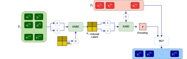
Figure 5: CIPNP architecture diagram

Table 16: CANP / BANP / CIPNP architecture (no latent path)

	Input	Layer(s)	Output
Cross Attention Encoder
	$\mathbf{X}_{t}\in\mathbb{R}^{B\times n\times 1\times 1}$	$\mathrm{MLP}$ (1 hidden layer, ReLU activation)	$\mathbf{Q}\in\mathbb{R}^{B\times n\times 128\times 1}$
	$\mathbf{X}_{c}\in\mathbb{R}^{B\times m\times 1\times 1}$	$\mathrm{MLP}$ (1 hidden layer, ReLU activation)	$\mathbf{K}\in\mathbb{R}^{B\times m\times 128}$
	$\mathbf{D}\in\mathbb{R}^{B\times m\times 2\times 1}$	(1) $\mathrm{MLP}$ (1 hidden layer, ReLU activation),	$\mathbf{V}=\mathbf{r}_{c}\in\mathbb{R}^{B\times m\times 128\times 1}$
		(2) $\mathrm{MAB}(\mathbf{D},\mathbf{D})$ (Self attn between data points)
		for CANP/BANP
		$\mathrm{MAB}(\mathbf{H}_{D},\mathbf{D})$ (XABD) for CIPNP
	$\mathbf{Q},\mathbf{K},\mathbf{V}$	Cross attn between query and context points	$\mathbf{r}\in\mathbb{R}^{B\times n\times 128\times 1}$
Pooling Encoder
	$\mathbf{D}\in\mathbb{R}^{B\times m\times 2\times 1}$	(1) $\mathrm{MLP}$ (1 hidden layer, ReLU activation),	$\mathbf{r}^{\prime}\in\mathbb{R}^{B\times n\times 128\times 1}$
		(2) $\mathrm{MAB}(\mathbf{D},\mathbf{D})$ (Self attn between data points)
		for CANP/BANP
		$\mathrm{MAB}(\mathbf{H}_{D},\mathbf{D})$ (XABD) for CIPNP
		(3) Mean pooling (on context points)
		(4) $\mathrm{MLP}$ (1 hidden layer, ReLU activation)
		(5) Repeat $n$ times
Decoder
	$\mathtt{concat}(\mathbf{X}_{t},\mathbf{r},\mathbf{r}^{\prime})$	(1) FC	$\phi\in\mathbb{R}^{B\times n\times 2}$
	$\in\mathbb{R}^{B\times n\times 257\times 1}$	(2) MLP (2 hidden layer, ReLU activation)
	$\phi$	chunk (splits input into 2 tensors of equal size)	$\mu,\Sigma\in\mathbb{R}^{B\times n\times 1}$
	$\mu,\Sigma$	Sampler	$\mathbf{Y}_{t}\in\mathbb{R}^{B\times n\times 1}$
			$\sim\mathcal{N}(\mu,\Sigma^{2})$

Table 17: ANP / IPNP architecture (latent path)

	Input	Layer(s)	Output
Cross Attention Encoder
Same as CANP / BANP / CIPNP (Table 16)
Latent Pooling Encoder
	$\mathbf{D}\in\mathbb{R}^{B\times m\times 2\times 1}$	(1) MLP (1 hidden layer, ReLU activation),	$\phi_{\mathbf{z}}^{\prime}\in\mathbb{R}^{B\times 256}$
		(2) $\mathrm{MAB}(\mathbf{D},\mathbf{D})$ (Self attn between data points)
		for ANP
		$\mathrm{MAB}(\mathbf{H}_{D},\mathbf{D})$ (XABD) for IPNP
		(3) Mean pooling (on context points)
		(4) MLP (1 hidden layer, ReLU activation)
	$\phi_{\mathbf{z}}$	chunk (splits input into 2 tensors of equal size)	$\mu_{\mathbf{z}},\Sigma_{\mathbf{z}}\in\mathbb{R}^{B\times 128\times 1}$
	$\mu_{\mathbf{z}},\Sigma_{\mathbf{z}}$	(1) Sampler
		(2) Repeat $n$ times	$\mathbf{z}\in\mathbb{R}^{B\times n\times 128\times 1}$
			$\sim\mathcal{N}(\mu_{\mathbf{z}},\Sigma^{2}_{\mathbf{z}})$
Decoder
	$\mathtt{concat}(\mathbf{X}_{t},\mathbf{r},\mathbf{z})$	(1) FC	$\phi\in\mathbb{R}^{B\times n\times 2}$
	$\in\mathbb{R}^{B\times n\times 257\times 1}$	(2) MLP (2 hidden layer, ReLU activation)
	$\phi$	chunk (splits input into 2 tensors of equal size)	$\mu,\Sigma\in\mathbb{R}^{B\times n\times 1}$
	$\mu,\Sigma$	Sampler	$\mathbf{Y}_{t}\in\mathbb{R}^{B\times n\times 1}$
			$\sim\mathcal{N}(\mu,\Sigma^{2})$

Qualitative Uncertainty Estimation Results

In Figure 6, we show baseline and inducing point NP models trained with context sizes $\in[64,128]$ and display the output of these models on new datasets with varying numbers of context points (4, 8, 16). We observe that the CIPNP and IPNP models better capture uncertainty in regions where context points have not been observed.

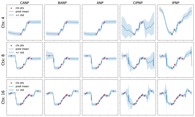
Figure 6: Predicted mean $\pm$ standard deviation of $\mathbf{y}$ for different NP models given varying context sizes: 4 (top), 8 (middle), and 16 (bottom).

Quantitative Calibration Results

To provide more quantitative results of how well our NP models capture uncertainty relative to baselines, we take models trained with context sizes $\in[64,128]$ and evaluate them on 1,000 evaluation batches each with number of targets points ranging from 4 to 64. We repeat this experiment three times with varying numbers of context points (4, 8, 16) available for each evaluation batch. In Figure 7, we see that in lower context regimes, CIPNP and IPNP models are better calibrated than the other baselines. As context size increases, the calibration of all the models deteriorates. This is further reflected in Table 18, where we display model calibration scores. Letting $CI$ be confidence intervals ranging from 0 to 1.0 by intervals of 0.1, $p_{CI}$ be the fraction of target labels that fall within confidence interval $CI,$ and $n$ be the number of confidence intervals, this calibration score is equal to:

$$\frac{1}{n}\sum_{CI=0}^{1}(p_{CI}-CI)^{2}$$ (1)

This score measures deviation of each model’s calibration plot from the $45^{\circ}$ line. Future work will explore the mechanisms that enable inducing point models to better capture uncertainty.

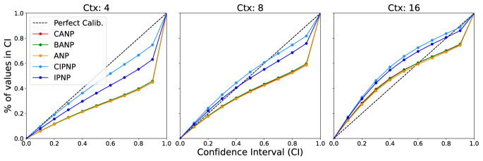
Figure 7: Calibration of NP models given varying context sizes: 4 (left), 8 (middle), and 16 (right).

Table 18: Calibration scores ($\downarrow$) for NP models across context sizes. Calibration score equals mean squared deviation from $45^{\circ}$ line of number of target points falling within confidence intervals ranging from 0 to 1 by intervals of 0.1, see Equation 1. Best (lowest) scores for each context size are bolded.

	Calibration score $\downarrow$
Context	CANP	BANP	ANP	CIPNP	IPNP
4	0.065	0.062	0.065	0.006	0.023
8	0.025	0.024	0.026	0.002	0.004
16	0.006	0.005	0.005	0.011	0.008

A.7 Ablation Analysis with Synthetic Experiment

We formulate a synthetic experiment where the model can only learn via XABD layers. First, we initialize a random binary matrix with 50% probability of 1’s, number of rows=5000, and number of columns=50. We set the last 20 columns to be target labels. Next, we copy a section of the dataset and divide it into three equal and disjoint parts for train query, val query, and test query. Since there is no correlation between the features and the target, the only way for the model to learn is via XABD layers (for a small dataset the model can also memorize the entire training dataset). This is similar to the synthetic experiment in NPT (Kossen et al., 2021), except that there is no relation between the features and target in our setup. We find that both default SPIN and SPIN with XABD only component achieves 100% binary classification accuracy, whereas SPIN with XABA only component achieves 70.01% classification accuracy, indicating the effectiveness of XABD component.

A.8 Qualitative Analysis for cross-attention

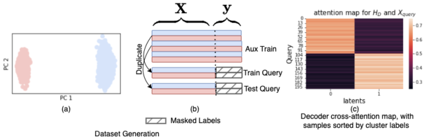
Figure 8: Synthetic Experiment analyzing cross-attention: (a)-(b) Data generating process to form two distinct clusters and data matrix with duplicate query samples and their labels masked. (c) Cross-attention map between query samples and the latent $H_{D}$

In order to understand what type of inducing points are learnt by the latent $H_{D}$, we formulate a toy synthetic dataset as shown in Figure 8. We start with two centroids consisting of binary strings with 120 bits and add bernoulli noise with $p=0.1$. We create the labels as another set of 4 bit binary strings and apply bernoulli noise with $p=0.1$. In this way we create a dataset with datapoints belonging to two separate clusters. Figure 8 (a) shows the projection of this dataset with two principal components when projected with PCA, highlighting that the dataset consists of two distinct clusters. We duplicate a part of this data to form the query samples so that they can be looked up from the latent via the cross attention mechanism. Figure 8 (b) shows the schematic of dataset with masked values for query labels. We use a SPIN model with a single XABD module, two induced latents ($h$=2) and input embedding dimension of 32 and inspect the cross-attention mechanism of the decoder. In Figure 8 (c), we plot the decoder cross attention map between test query and the induced latent and observe that the grouped query datapoints attend to the two latents consistent with the data generating clusters.

A.9 Image Classification Experiments

We conducted additional experiments comparing SPIN and NPT on two image classification datasets. Following NPT, we compare the results for image classification task using a linear patch encoder for MNIST and CIFAR10 dataset (which is the reason for the lower accuracies compared to using CNN-based encoders). Table 19 shows that for the linear patch encoder, SPIN and NPT both perform similarly in terms of accuracy, but SPIN uses far fewer parameters.

Table 19: Image Classification Experiments

Dataset	Approach	Classification Accuracy $\uparrow$	Peak GPU (GB)	Params Count
MNIST	NPT	97.92	1.33	33.34M
	SPIN	97.70	0.37	8.68M
CIFAR-10	NPT	68.20	18.81	900.36M
	SPIN	68.81	5.13	217.53M

A.10 Effect of number of induced points

We conducted sensitivity analysis of SPIN’s performance with respect to $h$ and $f$ and found that SPIN is fairly robust to the choice of these hyper-parameters, as evidenced by the low standard deviations in Table 20. This reflects redundancy in data and why attending to the entire dataset is inefficient.

Table 20: Effect of induced points $h,f$ for one genomic window (SNPs 424600-424700)

Induced Points $h$	Induced Points $f$	Pearson $R^{2}$ $\uparrow$	Peak GPU (GB)
$\{5\cdots 30\}$	10	94.03 $\pm{0.50}$	0.28 $\pm{0.}$
10	$\{5\cdots 30\}$	94.15 $\pm{0.25}$	0.32 $\pm{0.05}$
$\{5\cdots 30\}$	$\{5\cdots 30\}$	94.03 $\pm{0.28}$	0.32 $\pm{0.05}$

Appendix B Complexity Analysis

We provide time complexity for one gradient step, with $n_{l}$ as the number of layers, batch size $b$ equal to training dataset size $n$ during training, and one query sample during inference for transformer methods in Table 21. There are two operations that contribute heavily to the time complexity. First is computation of $Q.K^{T}$, second is the four times expansion in the feedforward layers. For NPT, the time complexity is given by maximum of ABD, ABA, and four times expansion in feedforward layers during ABD, that is $\max(n_{l}n^{2}de,n_{l}nd^{2}e,4n_{l}nd^{2}e^{2})$ during training and inference. Set Transformer consists of ISAB blocks that perform one cross-attention between latent and dataset to project into smaller space and a cross attention between dataset and latent to project back into input space for each layer. This results in complexity that is $\max(2n_{l}ndfe,2n_{l}nhfe,8n_{l}nd^{2}e^{2})$ during training and inference. For SPIN, the time complexity is given by maximum of XABD, XABA, ABLA, four times expansion in feedforward layers and one cross-attention for Predictor module. This can be formulated as $\max(n_{l}nhfe,n_{l}ndfe,n_{l}nf^{2}e,4n_{l}nf^{2}e,nhde,4nd^{2}e^{2})$. At inference, SPIN only uses the Predictor module, with the resultant complexity as $\max(hde,4d^{2}e^{2})$.

We note that during training for NPT, if $n$ >$4de$, then $Q.K^{T}$ computation in ABD dominates, otherwise the four times expansion of feedforward for ABD dominates. For Set Transformer, usually the four times expansion of feedforward dominates. For SPIN, depending on values for $n_{l},d,f,h,e$, different computations can dominate, however it is always linear in dataset size $n$. During inference SPIN’s time complexity is independent of number of layers $n_{l}$ and dataset size $n$ and depends entirely on inducing datapoints $h$, model embedding dimension $e$, and feature+target space $d$.

Table 21: Time Complexity

Approach	Time Complexity
	Train	Test
NPT	$\max(n_{l}n^{2}de,n_{l}nd^{2}e,$	$\max(n_{l}n^{2}de,n_{l}nd^{2}e,$
	$4n_{l}nd^{2}e^{2})$	$4n_{l}nd^{2}e^{2})$
STF	$\max(2n_{l}ndfe,2n_{l}nhfe,$	$\max(2n_{l}ndfe,2n_{l}nhfe,$
	$8n_{l}nd^{2}e^{2})$	$8n_{l}nd^{2}e^{2})$
SPIN	$\max(n_{l}nhfe,n_{l}ndfe,n_{l}nf^{2}e,$	$\max(hde,4d^{2}e^{2})$
	$4n_{l}nf^{2}e,nhde,4nd^{2}e^{2})$

Appendix C Code and Data Availability

UCI and Genomic Task Code

The experimental results for UCI and genomic task can be reproduced from here.

Neural Processes Code

The experimental results for the Neural Processes task can be reproduced from here.

Data for Genomics Experiment

The vcf file containing genotypes can be downloaded from 1000Genomes chromosome 20 vcf file. Additionally, the microarray used for genomics experiment can be downloaded from HumanOmni2.5 microarray. Beagle software, used as baseline, can be obtained from Beagle 5.1.

UCI Datasets

All UCI datasets can be obtained from UCI Data Repository.

References

- Achlioptas et al. (2001) Dimitris Achlioptas, Frank McSherry, and Bernhard Schölkopf. Sampling techniques for kernel methods. Advances in neural information processing systems, 14, 2001.
- Altman (1992) N. S. Altman. An introduction to kernel and nearest-neighbor nonparametric regression. The American Statistician, 46(3):175–185, 1992. doi: 10.1080/00031305.1992.10475879. URL https://www.tandfonline.com/doi/abs/10.1080/00031305.1992.10475879.
- Bach (2013) Francis Bach. Sharp analysis of low-rank kernel matrix approximations. In Conference on Learning Theory, pp. 185–209. PMLR, 2013.
- Belinkov (2022) Yonatan Belinkov. Probing classifiers: Promises, shortcomings, and advances. Computational Linguistics, 48(1):207–219, 2022.
- Beltagy et al. (2020) Iz Beltagy, Matthew E Peters, and Arman Cohan. Longformer: The long-document transformer. arXiv preprint arXiv:2004.05150, 2020.
- Bender et al. (2021) Emily M Bender, Timnit Gebru, Angelina McMillan-Major, and Shmargaret Shmitchell. On the dangers of stochastic parrots: Can language models be too big? In Proceedings of the 2021 ACM Conference on Fairness, Accountability, and Transparency, pp. 610–623, 2021.
- Bonetta et al. (2021) Giovanni Bonetta, Rossella Cancelliere, Ding Liu, and Paul Vozila. Retrieval-augmented transformer-xl for close-domain dialog generation. arXiv preprint arXiv:2105.09235, 2021.
- Brown et al. (2020) Tom Brown, Benjamin Mann, Nick Ryder, Melanie Subbiah, Jared D Kaplan, Prafulla Dhariwal, Arvind Neelakantan, Pranav Shyam, Girish Sastry, Amanda Askell, et al. Language models are few-shot learners. Advances in neural information processing systems, 33:1877–1901, 2020.
- Browning et al. (2018a) Brian L. Browning, Ying Zhou, and Sharon R. Browning. A one-penny imputed genome from next-generation reference panels. American Journal of Human Genetics, 2018a. doi: 10.1016/j.ajhg.2018.07.015.
- Browning et al. (2018b) Brian L Browning, Ying Zhou, and Sharon R Browning. A one-penny imputed genome from next-generation reference panels. The American Journal of Human Genetics, 103(3):338–348, 2018b.
- Cao et al. (2013) Yanshuai Cao, Marcus A Brubaker, David J Fleet, and Aaron Hertzmann. Efficient optimization for sparse gaussian process regression. Advances in Neural Information Processing Systems, 26, 2013.
- Choromanski et al. (2020) Krzysztof Marcin Choromanski, Valerii Likhosherstov, David Dohan, Xingyou Song, Andreea Gane, Tamas Sarlos, Peter Hawkins, Jared Quincy Davis, Afroz Mohiuddin, Lukasz Kaiser, et al. Rethinking attention with performers. In International Conference on Learning Representations, 2020.
- Clarke et al. (2016) Laura Clarke, Susan Fairley, Xiangqun Zheng-Bradley, Ian Streeter, Emily Perry, Ernesto Lowy, Anne-Marie Tassé, and Paul Flicek. The international Genome sample resource (IGSR): A worldwide collection of genome variation incorporating the 1000 Genomes Project data. Nucleic Acids Research, 45(D1):D854–D859, 09 2016. ISSN 0305-1048. doi: 10.1093/nar/gkw829. URL https://doi.org/10.1093/nar/gkw829.
- Compeau et al. (2011) Phillip E. C. Compeau, Pavel A. Pevzner, and Glenn Tesler. How to apply de bruijn graphs to genome assembly. Nature Biotechnology, 2011. doi: 10.1038/nbt.2023.
- Damianou & Lawrence (2013) Andreas Damianou and Neil D Lawrence. Deep gaussian processes. In Artificial intelligence and statistics, pp. 207–215. PMLR, 2013.
- Davis et al. (2011) Richard A Davis, Keh-Shin Lii, and Dimitris N Politis. Remarks on some nonparametric estimates of a density function. In Selected Works of Murray Rosenblatt, pp. 95–100. Springer, 2011.
- Delalleau et al. (2005) Olivier Delalleau, Yoshua Bengio, and Nicolas Le Roux. Efficient non-parametric function induction in semi-supervised learning. In International Workshop on Artificial Intelligence and Statistics, pp. 96–103. PMLR, 2005.
- Devlin et al. (2019) Jacob Devlin, Ming-Wei Chang, Kenton Lee, and Kristina Toutanova. BERT: Pre-training of deep bidirectional transformers for language understanding. In Proceedings of the 2019 Conference of the North American Chapter of the Association for Computational Linguistics: Human Language Technologies, Volume 1 (Long and Short Papers), pp. 4171–4186, Minneapolis, Minnesota, June 2019. Association for Computational Linguistics. doi: 10.18653/v1/N19-1423. URL https://aclanthology.org/N19-1423.
- Evans & Nair (2018) Trefor W. Evans and Prasanth B. Nair. Scalable gaussian processes with grid-structured eigenfunctions (gp-grief), 2018. URL https://arxiv.org/abs/1807.02125.
- Feng et al. (2023) Leo Feng, Hossein Hajimirsadeghi, Yoshua Bengio, and Mohamed Osama Ahmed. Latent bottlenecked attentive neural processes. In The Eleventh International Conference on Learning Representations, 2023. URL https://openreview.net/forum?id=yIxtevizEA.
- Frankle & Carbin (2018) Jonathan Frankle and Michael Carbin. The lottery ticket hypothesis: Finding sparse, trainable neural networks. In International Conference on Learning Representations, 2018.
- Friedman (2001) Jerome H. Friedman. Greedy function approximation: A gradient boosting machine. The Annals of Statistics, 29(5):1189 – 1232, 2001. doi: 10.1214/aos/1013203451. URL https://doi.org/10.1214/aos/1013203451.
- Garnelo et al. (2018) Marta Garnelo, Jonathan Schwarz, Dan Rosenbaum, Fabio Viola, Danilo J Rezende, SM Eslami, and Yee Whye Teh. Neural processes. arXiv preprint arXiv:1807.01622, 2018.
- Ghazvininejad et al. (2019) Marjan Ghazvininejad, Omer Levy, Yinhan Liu, and Luke Zettlemoyer. Mask-predict: Parallel decoding of conditional masked language models. In Proceedings of the 2019 Conference on Empirical Methods in Natural Language Processing and the 9th International Joint Conference on Natural Language Processing (EMNLP-IJCNLP), pp. 6112–6121, Hong Kong, China, November 2019. Association for Computational Linguistics. doi: 10.18653/v1/D19-1633. URL https://aclanthology.org/D19-1633.
- Glorot & Bengio (2010) Xavier Glorot and Yoshua Bengio. Understanding the difficulty of training deep feedforward neural networks. In Yee Whye Teh and Mike Titterington (eds.), Proceedings of the Thirteenth International Conference on Artificial Intelligence and Statistics, volume 9 of Proceedings of Machine Learning Research, pp. 249–256, Chia Laguna Resort, Sardinia, Italy, 13–15 May 2010. PMLR. URL https://proceedings.mlr.press/v9/glorot10a.html.
- Goyal et al. (2021) Anirudh Goyal, Aniket Didolkar, Alex Lamb, Kartikeya Badola, Nan Rosemary Ke, Nasim Rahaman, Jonathan Binas, Charles Blundell, Michael Mozer, and Yoshua Bengio. Coordination among neural modules through a shared global workspace. CoRR, abs/2103.01197, 2021. URL https://arxiv.org/abs/2103.01197.
- Goyal et al. (2022) Anirudh Goyal, Abram L. Friesen, Andrea Banino, Theophane Weber, Nan Rosemary Ke, Adria Puigdomenech Badia, Arthur Guez, Mehdi Mirza, Peter C. Humphreys, Ksenia Konyushkova, Laurent Sifre, Michal Valko, Simon Osindero, Timothy Lillicrap, Nicolas Heess, and Charles Blundell. Retrieval-augmented reinforcement learning, 2022. URL https://arxiv.org/abs/2202.08417.
- Grave et al. (2016) Edouard Grave, Armand Joulin, and Nicolas Usunier. Improving neural language models with a continuous cache. arXiv preprint arXiv:1612.04426, 2016.
- Graves et al. (2014) Alex Graves, Greg Wayne, and Ivo Danihelka. Neural turing machines. arXiv preprint arXiv:1410.5401, 2014.
- Grigsby et al. (2021) Jake Grigsby, Zhe Wang, and Yanjun Qi. Long-range transformers for dynamic spatiotemporal forecasting. arXiv preprint arXiv:2109.12218, 2021.
- Guu et al. (2020) Kelvin Guu, Kenton Lee, Zora Tung, Panupong Pasupat, and Ming-Wei Chang. Realm: Retrieval-augmented language model pre-training. arXiv preprint arXiv:2002.08909, 2020.
- Hearst et al. (1998) Marti A. Hearst, Susan T Dumais, Edgar Osuna, John Platt, and Bernhard Scholkopf. Support vector machines. IEEE Intelligent Systems and their applications, 13(4):18–28, 1998.
- Hensman et al. (2015) James Hensman, Alexander G Matthews, Maurizio Filippone, and Zoubin Ghahramani. Mcmc for variationally sparse gaussian processes. Advances in Neural Information Processing Systems, 28, 2015.
- Hinton (1989) Geoffrey E. Hinton. Connectionist learning procedures, 1989.
- Hoffmann et al. (2022) Jordan Hoffmann, Sebastian Borgeaud, Arthur Mensch, Elena Buchatskaya, Trevor Cai, Eliza Rutherford, Diego de Las Casas, Lisa Anne Hendricks, Johannes Welbl, Aidan Clark, et al. Training compute-optimal large language models. arXiv preprint arXiv:2203.15556, 2022.
- Izmailov & Kropotov (2016) Pavel Izmailov and Dmitry Kropotov. Faster variational inducing input gaussian process classification. arXiv preprint arXiv:1611.06132, 2016.
- Jaegle et al. (2021a) Andrew Jaegle, Sebastian Borgeaud, Jean-Baptiste Alayrac, Carl Doersch, Catalin Ionescu, David Ding, Skanda Koppula, Daniel Zoran, Andrew Brock, Evan Shelhamer, et al. Perceiver io: A general architecture for structured inputs & outputs. arXiv preprint arXiv:2107.14795, 2021a.
- Jaegle et al. (2021b) Andrew Jaegle, Felix Gimeno, Andrew Brock, Andrew Zisserman, Oriol Vinyals, and João Carreira. Perceiver: General perception with iterative attention. CoRR, abs/2103.03206, 2021b. URL https://arxiv.org/abs/2103.03206.
- Joshi et al. (2019) Mandar Joshi, Danqi Chen, Yinhan Liu, Daniel S. Weld, Luke Zettlemoyer, and Omer Levy. Spanbert: Improving pre-training by representing and predicting spans. CoRR, abs/1907.10529, 2019. URL http://arxiv.org/abs/1907.10529.
- Kaplan et al. (2020) Jared Kaplan, Sam McCandlish, Tom Henighan, Tom B Brown, Benjamin Chess, Rewon Child, Scott Gray, Alec Radford, Jeffrey Wu, and Dario Amodei. Scaling laws for neural language models. arXiv preprint arXiv:2001.08361, 2020.
- Katharopoulos et al. (2020) Angelos Katharopoulos, Apoorv Vyas, Nikolaos Pappas, and François Fleuret. Transformers are rnns: Fast autoregressive transformers with linear attention. In International Conference on Machine Learning, pp. 5156–5165. PMLR, 2020.
- Kendrew (2009) John Kendrew. The Encylopedia of Molecular Biology. John Wiley & Sons, 2009.
- Kim et al. (2018) Hyunjik Kim, Andriy Mnih, Jonathan Schwarz, Marta Garnelo, Ali Eslami, Dan Rosenbaum, Oriol Vinyals, and Yee Whye Teh. Attentive neural processes. In International Conference on Learning Representations, 2018.
- Kingma & Ba (2014) Diederik P Kingma and Jimmy Ba. Adam: A method for stochastic optimization. arXiv preprint arXiv:1412.6980, 2014.
- Kossen et al. (2021) Jannik Kossen, Neil Band, Clare Lyle, Aidan N. Gomez, Tom Rainforth, and Yarin Gal. Self-attention between datapoints: Going beyond individual input-output pairs in deep learning. CoRR, abs/2106.02584, 2021. URL https://arxiv.org/abs/2106.02584.
- Krizhevsky et al. (2012) Alex Krizhevsky, Ilya Sutskever, and Geoffrey E Hinton. Imagenet classification with deep convolutional neural networks. Advances in neural information processing systems, 25, 2012.
- Lee et al. (2018) Juho Lee, Yoonho Lee, Jungtaek Kim, Adam R. Kosiorek, Seungjin Choi, and Yee Whye Teh. Set transformer. CoRR, abs/1810.00825, 2018. URL http://arxiv.org/abs/1810.00825.
- Lee et al. (2020) Juho Lee, Yoonho Lee, Jungtaek Kim, Eunho Yang, Sung Ju Hwang, and Yee Whye Teh. Bootstrapping neural processes. Advances in neural information processing systems, 33:6606–6615, 2020.
- Li & Stephens (2003) Na Li and Matthew Stephens. Modeling linkage disequilibrium and identifying recombination hotspots using single-nucleotide polymorphism data. Genetics, 165(4):2213–2233, 2003.
- Li et al. (2009) Yun Li, Cristen Willer, Serena Sanna, and Gonçalo Abecasis. Genotype imputation. Annual review of genomics and human genetics, 10:387–406, 2009.
- Lou et al. (2021) Runyang Nicolas Lou, Arne Jacobs, Aryn P Wilder, and Nina Overgaard Therkildsen. A beginner’s guide to low-coverage whole genome sequencing for population genomics. Molecular Ecology, 30(23):5966–5993, 2021.
- Maarala et al. (2020) Altti Ilari Maarala, Kalle Pärn, Javier Nuñez-Fontarnau, and Keijo Heljanko. Sparkbeagle: Scalable genotype imputation from distributed whole-genome reference panels in the cloud. In Proceedings of the 11th ACM International Conference on Bioinformatics, Computational Biology and Health Informatics, pp. 1–8, 2020.
- Nguyen et al. (2020) Timothy Nguyen, Zhourong Chen, and Jaehoon Lee. Dataset meta-learning from kernel ridge-regression. In International Conference on Learning Representations, 2020.
- Nguyen & Salazar (2019) Toan Q. Nguyen and Julian Salazar. Transformers without tears: Improving the normalization of self-attention. In Proceedings of the 16th International Conference on Spoken Language Translation, Hong Kong, November 2-3 2019. Association for Computational Linguistics. URL https://aclanthology.org/2019.iwslt-1.17.
- Nguyen & Grover (2022) Tung Nguyen and Aditya Grover. Transformer neural processes: Uncertainty-aware meta learning via sequence modeling. arXiv preprint arXiv:2207.04179, 2022.
- Peters et al. (2018) Matthew E. Peters, Mark Neumann, Mohit Iyyer, Matt Gardner, Christopher Clark, Kenton Lee, and Luke Zettlemoyer. Deep contextualized word representations. In Proceedings of the 2018 Conference of the North American Chapter of the Association for Computational Linguistics: Human Language Technologies, Volume 1 (Long Papers), pp. 2227–2237, New Orleans, Louisiana, June 2018. Association for Computational Linguistics. doi: 10.18653/v1/N18-1202. URL https://aclanthology.org/N18-1202.
- Rae et al. (2021) Jack W Rae, Sebastian Borgeaud, Trevor Cai, Katie Millican, Jordan Hoffmann, Francis Song, John Aslanides, Sarah Henderson, Roman Ring, Susannah Young, et al. Scaling language models: Methods, analysis & insights from training gopher. arXiv preprint arXiv:2112.11446, 2021.
- Rahimi & Recht (2007) Ali Rahimi and Benjamin Recht. Random features for large-scale kernel machines. Advances in neural information processing systems, 20, 2007.
- Ramesh et al. (2022) Aditya Ramesh, Prafulla Dhariwal, Alex Nichol, Casey Chu, and Mark Chen. Hierarchical text-conditional image generation with clip latents. arXiv preprint arXiv:2204.06125, 2022.
- Rasmussen (2003) Carl Edward Rasmussen. Gaussian processes in machine learning. In Summer school on machine learning, pp. 63–71. Springer, 2003.
- Rubinacci et al. (2020) Simone Rubinacci, Olivier Delaneau, and Jonathan Marchini. Genotype imputation using the positional burrows wheeler transform. PLOS Genetics, 2020. doi: 10.1371/journal.pgen.1009049.
- Santoro et al. (2016) Adam Santoro, Sergey Bartunov, Matthew Botvinick, Daan Wierstra, and Timothy Lillicrap. Meta-learning with memory-augmented neural networks. In International conference on machine learning, pp. 1842–1850. PMLR, 2016.
- Snelson & Ghahramani (2005) Edward Snelson and Zoubin Ghahramani. Sparse gaussian processes using pseudo-inputs. In Y. Weiss, B. Schölkopf, and J. Platt (eds.), Advances in Neural Information Processing Systems, volume 18. MIT Press, 2005. URL https://proceedings.neurips.cc/paper/2005/file/4491777b1aa8b5b32c2e8666dbe1a495-Paper.pdf.
- Titsias (2009) Michalis Titsias. Variational learning of inducing variables in sparse gaussian processes. In David van Dyk and Max Welling (eds.), Proceedings of the Twelth International Conference on Artificial Intelligence and Statistics, volume 5 of Proceedings of Machine Learning Research, pp. 567–574, Hilton Clearwater Beach Resort, Clearwater Beach, Florida USA, 16–18 Apr 2009. PMLR. URL https://proceedings.mlr.press/v5/titsias09a.html.
- Tolstikhin et al. (2021) Ilya O. Tolstikhin, Neil Houlsby, Alexander Kolesnikov, Lucas Beyer, Xiaohua Zhai, Thomas Unterthiner, Jessica Yung, Andreas Steiner, Daniel Keysers, Jakob Uszkoreit, Mario Lucic, and Alexey Dosovitskiy. Mlp-mixer: An all-mlp architecture for vision. CoRR, abs/2105.01601, 2021. URL https://arxiv.org/abs/2105.01601.
- Vaswani et al. (2017) Ashish Vaswani, Noam Shazeer, Niki Parmar, Jakob Uszkoreit, Llion Jones, Aidan N Gomez, Łukasz Kaiser, and Illia Polosukhin. Attention is all you need. Advances in neural information processing systems, 30, 2017.
- Wang et al. (2020) Sinong Wang, Belinda Z Li, Madian Khabsa, Han Fang, and Hao Ma. Linformer: Self-attention with linear complexity. arXiv preprint arXiv:2006.04768, 2020.
- Wang et al. (2016) Yali Wang, Marcus Brubaker, Brahim Chaib-Draa, and Raquel Urtasun. Sequential inference for deep gaussian process. In Artificial Intelligence and Statistics, pp. 694–703. PMLR, 2016.
- Wilson & Nickisch (2015) Andrew Wilson and Hannes Nickisch. Kernel interpolation for scalable structured gaussian processes (kiss-gp). In International conference on machine learning, pp. 1775–1784. PMLR, 2015.
- Wilson et al. (2015) Andrew Gordon Wilson, Christoph Dann, and Hannes Nickisch. Thoughts on massively scalable gaussian processes. arXiv preprint arXiv:1511.01870, 2015.
- Wilson et al. (2016) Andrew Gordon Wilson, Zhiting Hu, Ruslan Salakhutdinov, and Eric P Xing. Deep kernel learning. In Artificial intelligence and statistics, pp. 370–378. PMLR, 2016.
- Wiseman & Stratos (2019) Sam Wiseman and Karl Stratos. Label-agnostic sequence labeling by copying nearest neighbors. In Proceedings of the 57th Annual Meeting of the Association for Computational Linguistics, pp. 5363–5369, Florence, Italy, July 2019. Association for Computational Linguistics. doi: 10.18653/v1/P19-1533. URL https://aclanthology.org/P19-1533.
- (73) Wrayner. Human omni marker panel. URL https://www.well.ox.ac.uk/~wrayner/strand/.
- Xiong et al. (2021) Yunyang Xiong, Zhanpeng Zeng, Rudrasis Chakraborty, Mingxing Tan, Glenn Fung, Yin Li, and Vikas Singh. Nyströmformer: A nystöm-based algorithm for approximating self-attention. In Proceedings of the… AAAI Conference on Artificial Intelligence. AAAI Conference on Artificial Intelligence, volume 35, pp. 14138. NIH Public Access, 2021.
- Yang et al. (2018) Zhilin Yang, Peng Qi, Saizheng Zhang, Yoshua Bengio, William Cohen, Ruslan Salakhutdinov, and Christopher D. Manning. HotpotQA: A dataset for diverse, explainable multi-hop question answering. In Proceedings of the 2018 Conference on Empirical Methods in Natural Language Processing, pp. 2369–2380, Brussels, Belgium, October-November 2018. Association for Computational Linguistics. doi: 10.18653/v1/D18-1259. URL https://aclanthology.org/D18-1259.
- Zaheer et al. (2020) Manzil Zaheer, Guru Guruganesh, Kumar Avinava Dubey, Joshua Ainslie, Chris Alberti, Santiago Ontanon, Philip Pham, Anirudh Ravula, Qifan Wang, Li Yang, et al. Big bird: Transformers for longer sequences. Advances in Neural Information Processing Systems, 33:17283–17297, 2020.
- Zhang et al. (2019) Michael Zhang, James Lucas, Jimmy Ba, and Geoffrey E Hinton. Lookahead optimizer: k steps forward, 1 step back. Advances in Neural Information Processing Systems, 32, 2019.