There and back again: understanding the critical properties of backsplash galaxies

Abstract

Backsplash galaxies are galaxies that once resided inside a cluster, and have migrated back oustide as they move towards the apocentre of their orbit. The kinematic properties of these galaxies are well understood, thanks to the significant study of backsplashers in dark matter-only simulations, but their intrinsic properties are not well constrained due to modelling uncertainties in sub-grid physics, ram pressure stripping, dynamical friction, and tidal forces. In this paper, we use the IllustrisTNG300-1 simulation, with a baryonic resolution of $M_{\rm b}\approx 1.1\times 10^{7}$ M_⊙, to study backsplash galaxies around 1302 isolated galaxy clusters with mass $10^{13.0}<M_{\rm 200,mean}/{\rm M}_{\odot}<10^{15.5}$. We employ a decision tree classifier to extract features of galaxies that make them likely to be backsplash galaxies, compared to nearby field galaxies, and find that backsplash galaxies have low gas fractions, high mass-to-light ratios, large stellar sizes, and low black hole occupation fractions. We investigate in detail the origins of these large sizes, and hypothesise their origins are linked to the tidal environments in the cluster. We show that the black hole recentreing scheme employed in many cosmological simulations leads to the loss of black holes from galaxies accreted into clusters, and suggest improvements to these models. Generally, we find that backsplash galaxies are a useful population to test and understand numerical galaxy formation models due to their challenging environments and evolutionary pathways that interact with poorly constrained physics.

1 Introduction

Understanding the assembly and composition of galaxy clusters has been a topic of research for decades. Within the Lambda-CDM cosmological paradigm, these massive systems are understood to be hierachically created from many smaller substructures. Galaxy clusters are assembled when many subhaloes, containing galaxies, accrete together to form self-bound strucutres of halo mass $M_{\rm 200,mean}>10^{13}$ M_⊙. Here $M_{\rm 200,mean}$ is defined as the mass enclosed within $R_{\rm 200,mean}$, the radius enclosing 200 times the mean density of the Universe at that epoch. What happens when one of these galaxies leaves the cluster again? Is such a process possible? If so, what do these galaxies look like and why? This paper explores the life and times of such ‘backsplash’ galaxies, through the use of the TNG300 cosmological galaxy formation simulation, and attempts to address these open questions.

Backsplash galaxies were first studied in early theoretical work by Balogh et al. (2000), using mass accretion histories from N-body simulations and an analytical model to explain star formation gradients in the outskirts of galaxy clusters. The general understanding was that galaxy clusters quench galaxies, and galaxies that fall into clusters have a chance of ‘bouncing’ back out of the clusters to an apocentre greater than the virial radius $R_{\rm vir}$, provided they have enough orbital energy. Hence, in the outskirts of the clusters, star forming galaxies would be mixed with these quenched backsplash galaxies, with the number of backsplashers dropping off with radius but the density of the infalling population remaining relatively constant with radius, giving rise to a gradient in star formation activity even further out than $R_{\rm vir}$.

This early work was complimented by theoretical and observational studies by Mamon et al. (2004) and Sanchis et al. (2004) looking at neutral hydrogen (HI) deficient galaxies near the Virgo cluster. It was not until Gill et al. (2005), however, that the term ‘backsplash galaxy’ was actually coined, which was the first systematic study evaluating the expected kinematic (i.e. including velocity-space information) properties of these interlopers. Gill et al. (2005) used N-body simulations to predict that 50% of galaxies in the range $1<R/R_{\rm vir}<2$ would be backsplash galaxies, and that these galaxies had close pericentre passages to the centre of the cluster before rebounding. Within a month, Kilborn et al. (2005) provided observational evidence of two HI-poor galaxies within this radial range around the NGC 1566 group, further suggesting that such galaxies could indeed exist in the real Universe.

Later theoretical and observational work by Ludlow et al. (2009), Hansen et al. (2009), Knebe et al. (2011), and Bahé et al. (2013), using a variety of techniques, cemented the idea that backsplash galaxies are a cause of colour gradients in galaxies out to multiple times $R_{\rm 200,mean}$. Notably, Knebe et al. (2011) found that the processing and production of backsplash subhaloes even occurs on dwarf galaxy scales, in simulations of the local group.

Much of the work investigating the interaction of cluster galaxies and their hosts has employed the use of semi-analytical models, which use a base dark matter-only simulation to generate accretion histories, followed by an analytical model for studying the baryonic component. Simulating galaxy clusters with a full hydrodynamical treatment is incredibly complex, with authors turning to zoom simulations (where only a small fraction of the volume is hydrodynamically active), or sacrificing numerical resolution significantly (Barnes et al., 2017; McCarthy et al., 2017; Ragone-Figueroa et al., 2018; Haggar et al., 2020; Bassini et al., 2020). Additionally, the processes involved in the evolution and production of backsplash galaxies, including ram-pressure stripping and dynamical friction, are still not fully understood (Simpson et al., 2018; van den Bosch & Ogiya, 2018). The subhaloes that are able to rebound from the cluster are typically of lower mass, with subhaloes with total halo mass $M_{\rm H}/M_{\rm 200,mean}>0.01$ strongly impacted by dynamical friction leading to rapid merging with the central galaxy in the cluster (Bakels et al., 2021).

Despite these potential numerical pitfalls, there has recently been renewed interest in backsplash galaxies as a potential formation mechanism of ultra-diffuse galaxies (UDGs, see e.g. van Dokkum et al., 2015; Koda et al., 2015; Tremmel et al., 2020; Jones et al., 2021). UDGs are low surface-brightness dwarf galaxies, typically with larger stellar sizes than field dwarfs. Many UDGs are located near clusters and have intrinsic properties similar to those expected of backsplash galaxies (Benavides et al., 2021; Trujillo, 2021). Additionally, the challenges of simulating backsplash galaxies make them an excellent testing ground for the accuracy of numerical models. Modern galaxy formation models are currently able to reproduce a statistcally representative sample of simulated galaxies, but typically struggle to reproduce the observed properties of ‘extremophile’ galaxies that reside in extreme environments (Somerville & Davé, 2015; Vogelsberger et al., 2020; de los Rios et al., 2021).

Recently, Farid et al. (2022) used a random forest algorithm to classify the membership properties of cluster galaxies, and was able to perform such classification with high ($>80\%$) accuracy when employing phase-space information. In practice, however, phase-space information is difficult to generate as typically only velocities along the line of sight (from redshift information) can be observed. To reach this accuracy, they additionally augment their model by using the specific star formation rate (sSFR) of galaxies, but a notable inaccuracy in their model is that they underpredict the classification of orbiting galaxies at radii $1.0<R/R_{\rm 200,mean}<2.0$ (i.e. their model underclassifies backsplash galaxies) when using a hard classification scheme.

In this paper, we aim to classify galaxies near clusters into two categories, infalling (never within $R_{\rm 200,mean}$ of a cluster), and backsplash (has been within $R_{\rm 200,mean}$ of a cluster, but are now further away). We use the IllustrisTNG suite of cosmological galaxy formation simulations, and employ the largest volume simulation with a comoving box-size of $(300{\rm Mpc})^{3}$. Through the development of a classification model for the galaxies based upon their intrinsic properties, we aim to identify which features of backsplash galaxies make them unique from the general field population, and use these features to understand their formation and evolution.

The rest of this paper is organised as follows: In §2, we give a brief overview of the IllustrisTNG model and simulations. In §3, we describe our cluster and galaxy selection process, and discuss some basic properties of backsplash galaxies in the TNG model. In §4, we use a decision tree machine learning model to understand which properties of galaxies can be used to classify them as backsplashers or infalling. In §5, we discuss the origins of the larger sizes of backsplash galaxies, and in §6, we aim to understand the low supermassive back hole occupation fraction and masses in backsplash galaxies. Finally, in §7, we give concluding remarks.

2 The IllustrisTNG Simulation Suite

In this work we use simulations from the IllustrisTNG suite of cosmological galaxy formation simulations, released in Nelson et al. (2019). In particular, we use data from the public release of the IllustrisTNG300-1 simulation (Pillepich et al., 2018b; Springel et al., 2018; Nelson et al., 2018; Naiman et al., 2018; Marinacci et al., 2018). The simulation is henceforth referred to as TNG300, and follows a (300 Mpc)³ comoving, representative, volume of universe from just after the big bang down to the present day at $z=0$. All results in this paper should be assumed to be at $z=0$ unless otherwise stated.

The TNG300 volume initially contains $2500^{3}$ gas cells of target mass $1.1\times 10^{7}$ M_⊙ and $2500^{3}$ dark matter particles of fixed mass $5.9\times 10^{7}$ M_⊙. These particles are evolved over cosmic time using the continuum magnetohydrodynamics (MHD) and gravity code Arepo (Springel, 2011; Weinberger et al., 2020). Arepo is a massively parallel code that uses a moving Voronoi mesh coupled with a finite volume method to compute forces and fluxes originating from MHD, along with a combined tree and particle mesh (TreePM) method to calculate perodic and non-periodic self-gravitational forces.

Coupled to the base Arepo code is the IllustrisTNG galaxy formation sub-grid model, a sucessor to the Illustris galaxy formation model (Vogelsberger et al., 2013; Vogelsberger et al., 2014b). Galaxy formation sub-grid models are required to include physics that occurs below the resolution scale. Within the TNG model, there are prescriptions for radiative gas cooling (Wiersma et al., 2009), star formation and stellar feedback (Springel & Hernquist, 2003), and (supermassive) black hole formation and active galactic nuclei feedback (Weinberger et al., 2017). The simulation was performed assuming a cosmology conforming to the 2015 release from the Planck satellite, with $\Omega_{\Lambda,0}=0.6911$, $\Omega_{\rm m,0}=0.3089$, $\Omega_{\rm b,0}=0.0486$, $\sigma_{8}=0.8159$, $n_{\rm s}=0.9667$, and $h=0.6774$, with the symbols having their usual meaning (Planck Collaboration et al., 2016). More information on the specific implementation details is available in the data release paper and associated webpages (Nelson et al., 2019).

Here we primarily use reduced data from the available SubFind group catalouges. SubFind primarily uses a friends-of-friends (FoF) algorithm (Springel et al., 2005; Dolag et al., 2009) to idenfify haloes and their constituent subhaloes. In TNG300, the initial FoF search uses a typical default linking length of $b=0.2$, before the SubFind galaxy finder algorithm is ran. For each of the 100 TNG300 snapshots, a group catalogue is created containing properties of galaxies (subhaloes) and groups (haloes). These group catalogues are used, along with the L-HaloTree algorithm (Springel et al., 2005), to follow the paths of individual structures over time and build up a merger tree of haloes.

Figure 1: Shows a $10^{15}$ ${\rm M}_{\odot}$ cluster from the Illustris TNG300 simulation. The background image shows the stellar density (luminance of the image; i.e. brighter regions have a higher projected stellar density), with the colour showing the mean, mass-weighted, $U-V$ colour along the line of sight. Each ring shows a galaxy that currently resides outside the radius $R_{\rm 200,mean}$ (dotted white line), with the rings coloured by the $U-V$ colour of the substructure. If the ring is dotted, it represents an infalling galaxy (note that these are typically bluer), and if solid it is a backsplash galaxy. The white dashed line shows the maximal (3D) radius that a backsplash substructure can be found at for this cluster ($R_{\rm sub,max}$). Finally, the thin light lines show the paths of the highlighted galaxies.

3 Selecting Backsplash Galaxies

As we were motivated to study backsplash galaxies by the study of the splashback radius of galaxy clusters, we use the same sample of clusters as in O’Neil et al. (2022). These are chosen to be isolated galaxy clusters with a mass $M_{\rm 200,mean}>10^{13}$ M_⊙. This sample is constructed by ensuring that the clusters are the most massive within $10R_{\rm 200,mean}$ of any nearby cluster. This is ensured by, for every candidate in the $z=0$ snapshot, looping over all other candidates within $10R_{\rm 200,mean}$. In this loop, if any nearby candidate has a mass lower than the cluster being considered, it is marked as removed from the sample.

The advantage of this approach (as compared to only looping over nearby members and asserting there must be no halo of greater mass) is that if, say, there is a $M_{\rm 200,mean}=10^{13}$ M_⊙ galaxy cluster near a $M_{\rm 200,mean}=10^{15}$ M_⊙ cluster, the lower mass one (which will be significantly impacted by the nearby, more massive, cluster, despite the $10^{13}$ M_⊙ cluster not ‘seeing’ the $10^{15}$ M_⊙ cluster in its radial search) is not included in our sample.

For each isolated cluster we then employ the L-HaloTree merger trees, and track the first progenitor (most massive subhalo) of the cluster back in time. To ensure that we are able to accurately track the movement of the cluster back in time (and as such reconstruct the paths of its satellites accurately), we apply an additional set of constraints:

• The first progenitor of the cluster must be traceable through at least the most recent 40 snapshots (at least back to $z=0.7$, or approximately half a Hubble time). This ensures we have a stable enough cluster to follow infalling galaxies for at least a handful of cluster crossing times (typically $t_{\rm cross}\approx 1-2$ Gyr).

• The cluster must not move more than 10 Mpc per Gyr (comoving) relative to the fixed box, to ensure that it corresponds to the local potential maximum. This works alongside our isolated galaxy constraint to ensure that as few as possible backsplash galaxies are transferred between clusters and experience interactions with more than one cluster. In particular, this could skew our results since galaxies that have passed through a different cluster would not be identified as backsplash despite being subject to a cluster environment similar to backsplash galaxies of its current host halo.

• In a similar fashion, there must be less than a 0.5 Mpc offset between where the cluster is predicted to be based upon its velocity and time between snapshots relative to its position in the next snapshot.

This set of constraints esnures that the clusters move smoothly, and are the most dominant halo within their local neighborhood, to ensure a clean sample of infalling and backsplashing galaxies. The final selection of clusters rejects around 100 compared to O’Neil et al. (2022), with 1302 clusters remaining.

To track the galaxies resident in, and near, these clusters, we again employ the L-HaloTree merger trees. We identify all galaxies within the range $1<R_{\rm 200,mean}<10$ of each cluster at $z=0$, and track their first progenitor (whether it is bound to, enters, or is assoicated with the merger tree of the cluster or not) back as far as it can be identified by the tree. We apply a stellar mass cut of $M_{*}>10^{8}$ M_⊙, only tracking substructure that has a mass higher than this at $z=0$ back in time, to ensure that all substructure would be visible and to ease computational load, though such a tracking procedure is not particularly computationally complex.

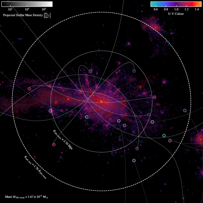
We then assign galaxies a label of ‘backsplash’ or ‘infalling’ based on whether they have come within $R_{\rm 200,mean}$ of the cluster (at the relevant redshift) at any time. In Fig. 1, we show the tracks of some example backsplash and infalling galaxies, alongside a massive galaxy cluster ($M_{\rm 200,mean}=1.67\times 10^{15}$ M_⊙). The infalling galaxies, indicated by dotted circles, have yet to interact with the cluster (note that this is a projection along the $z$-axis of the simulation), whereas the backsplash galaxies (indicated by solid rings) have had a close periapsis with the cluster. Notable in this image is the dense prescence of galaxies on the opposing side of the cluster to the infalling filament (on the left of the image). We also identify the maximal radius at which any backsplashing substructure is found at, $R_{\rm sub,max}$.

From Fig. 1 it is clear that we expect some divergence in the properties of backsplash and infalling galaxies. It is already clear that the infalling galaxies are much bluer, with backsplash galaxies being red (i.e. a high $U-V$ colour).

Figure 2: Shows properties of backsplash galaxies as a function of host cluster mass. In all panels, the blue dots represent the position of a single cluster in the plane, with the red error bars showing the 16th, 50th, and 84th percentile ranges (bottom, point, top) for clusters binned in 8 equally log-spaced bins between $10^{13}\leq M_{\rm 200,mean}/{\rm M}_{\odot}\leq 10^{15}$. Top panel: The fraction of subhaloes in the range $1.0<R/R_{\rm 200,mean}<2.0$ that are classified as backsplash galaxies. Middle panel: The total number of backsplash galaxies within this range as a function of cluster mass. This only edges above a median of one in clusters with $M_{\rm 200,mean}>10^{13.5}~{}{\rm M}_{\odot}$. Bottom panel: The maximum radius at which a backsplash galaxy is found for all clusters.

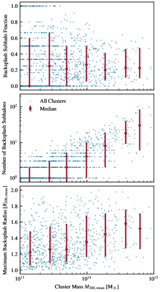
Fig. 2 shows some basic properties of backsplash galaxies as they scale with the cluster mass $M_{\rm 200,mean}$. The top panel shows the fraction of all subhaloes within the range $1<R/R_{\rm 200,mean}<2$ that are backsplashers, which is consistenly around 30% across the cluster mass range. Our backsplash fraction is lower than previously studied simulations, with Gill et al. (2005) finding a backsplash fraction of 50%, and Haggar et al. (2020) finding that the backsplash fraction is of order 60%. Haggar et al. (2020) uses significantly higher mass clusters ($5\times 10^{14}<M_{\rm 200,crit}/{\rm M}_{\odot}<3\times 10^{15}$) than this work, and apply a much higher mass cut on their galaxies (with $M_{\rm*}>10^{9.5}$ M_⊙). Additionally, they find that the backsplash fraction depends on the relaxation of the cluster, with the most relaxed clusters having backsplash fractions less than 20%. Our isolation and tracking criteria for our clusters, required as they live in live, full volume simulations (as opposed to zoom-in simulations of clusters like TheThreeHundred sample), likely selects more relaxed clusters. As we are mainly interested in the properties of the backsplash galaxies themselves, rather than their host clusters, we defer further investigation to potential future work.

The central panel shows that below cluster masses of $M_{\rm 200,mean}=10^{14}$ M_⊙, a very low fraction of clusters have any backsplash galaxies at all, and the number of backsplash subhaloes scales roughly linearly with cluster mass. This is primarily due to two factors: their smaller values of $R_{\rm 200,mean}$ leading to a smaller volume within which backsplash galaxies may reside, and their lower density environments.

Finally, the bottom panel of Fig. 2 shows the distribution of the maximal radii at which backsplash subhaloes are found ($R_{\rm sub,max}$ in Fig. 1). In this panel, clusters are not included if they do not have any backsplash subhaloes. We find that the maximal radius, relative to $R_{\rm 200,mean}$, increases with cluster mass. This is particularly notable as the splashback radius $R_{\rm sp}$ has been shown by many authors, in particular O’Neil et al. (2021) for this sample, to decrease with cluster mass. Typical values of the splashback radius are roughly $R_{\rm sp}/R_{\rm 200,mean}\approx 1.1-1.2$, as measured based upon the dark matter profiles, trending down with cluster mass. That there are many galaxies outside of the typical splashback radius for these clusters is not particularly surprising; the splashback radius should be the point at which backsplash galaxies and infalling galaxies are at rough equipartition (assuming galaxy number density traces mass density). We attribute the increase in maximal backsplash galaxy radius with mass to the better sampling that these haloes have, with them simply being more likely to find a galaxy out at this radius.

Figure 3: Top panel: The number density profile of all galaxies with $M_{*}>10^{8}~{}{\rm M}_{\odot}$ in our sample, stacked for all clusters in the sample. The dark blue line shows the profile of all galaxies, with the vertical black dashed line deliniating the point at which backsplash galaxies are classifed ($R_{\rm 200,mean}$). Outside this radius, the infalling galaxies (light blue) and backsplash galaxies (red) have their profiles shown separately, with the infalling galaxies tracing an almost constant density, and the density of the backsplash galaxies falling off rapidly outside of the cluster. Bottom Panel: The volume-weighted fraction of backsplash and infalling galaxies as a function of radius. Horizontal dotted lines are shown at common percentile ranges to guide the eye. By $1.6R_{\rm 200,mean}$ fewer than 10% of galaxies are backsplash, making attemtps to classify galaxies outside this radius infeasible. The dashed, lighter, lines shown in the background show the cumulative fraction of galaxies in each classification out to this radius (i.e. the fraction of galaxies with radius $r<R$ that are backsplash or infalling galaxies). The equal partition between these two classifications is reached at $1.24R_{\rm 200,mean}$ (grey dot-dash line)

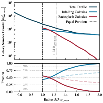
Fig. 3 shows the radial number density profile of galaxies, stacked across all clusters in our sample, and resacled by $R_{\rm 200,mean}$. Even by $R=1.1R_{\rm 200,mean}$, galaxies that are infalling become more abundant, indicating just how rare backsplash galaxies are. We indicate that within the annulus of $1.0<R/R_{\rm 200,mean}<1.24$ the density of backsplash galaxies and infalling galaxies are equal. Bakels et al. (2021) finds that the radius at which backsplashing and infalling subhaloes have equal density is at around $R/R_{\rm 200,crit}\approx 1.8$ (their Fig. 3), similar to our $R/R_{\rm 200,mean}\approx 1.1$, making our results consistent despite their more complex tracking procedure. We find little evolution in the equipartition radius with host cluster mass, with it placed at $R/R_{\rm 200,mean}=1.26$ and $1.24$ for clusters in mass ranges $10^{13}<M_{\rm 200,mean}/{\rm M}_{\odot}<10^{14}$ and $10^{14}<M_{\rm 200,mean}/{\rm M}_{\odot}<10^{15}$ respectively, and hence only show the stacked profile across our entire cluster sample.

Fig. 3 shows that the infalling component has a near-constant density across the radial range, with the backsplash (orbital) component falling off rapidly with radius. This suggests that looking for galaxies bound to the cluster much further away than $R/R_{\rm 200,mean}\approx 1.5$ is unlikely to yield a large number of results. Further, it suggests that galaxies found this far away are unlikely to have been processed by the cluster previously, meaning that in all liklehood their properties are determined by their internal evolution rather than their environment.

Figure 4: The radial velocity distributions for galaxies within $1<R/R_{\rm 200,mean}<2$, split by infalling/backsplash category (blue and red points, respectively), split by halo mass (different panels). Radial velocities are binned in 32 equally spaced linear bins between $-2000~{}{\rm km}~{}{\rm s}^{-1}\leq v_{\rm r}\leq 1500~{}{\rm km}~{}{\rm s}^{-1}$. The background lines show gaussian fits to the binned data to guide the eye. Infalling galaxies have, almost universally, a negative radial velocity (as expected). Backsplash galaxies have a gaussian distribution of radial velocities centred around, approximately, zero; at higher masses, though, the backsplash galaxies are biased to having a mean velocity greater than zero (i.e. there are more galaxies on their way back out of the cluster than falling back in). Notably the results remain qualitatively consistent (other than the relative abundances) when only considering galaxies within $R<1.24R_{\rm 200,mean}$.

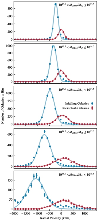
In Fig. 4 we show the radial velocity distributions of the cluster galaxies in our sample, split by host cluster halo mass. Here we calculate radial velocity disregarding the negligeable Hubble flow component (of order 100 km s^-1) to better understand the gravitational dynamics at play in clusters. This becomes non-negligeable for the highest mass clusters that host galaxies at the largest radii in the lower panels, meaning that there is an offset in the central velocity for backsplash galaxies. The radial velocity is calculated in the rest frame of the cluster and is given by

$$v_{\rm r}=\frac{(\vec{v}_{\rm gal}-\vec{v}_{\rm clu})\cdot(\vec{x}_{\rm gal}-\vec{x}_{\rm clu})}{|\vec{x}_{\rm gal}-\vec{x}_{\rm clu}|},$$ (1)

where here $\vec{v}$ and $\vec{x}$ are the physical velocity and position of the cluster and galaxy (subscripts clu and gal respectively) relative to the simulation box.

We see that the velocities of backsplash galaxies generally follow a normal distribution around zero, with roughly equal numbers of galaxies on their way out ($v_{\rm r}>0$) as in ($v_{\rm r}<0$) to the cluster. The infalling galaxies, on the other hand, almost universally are falling into the cluster ($v_{\rm r}<0$, note that we did not make a velocity-based cut in our criterion for infalling galaxies, just that they must be near a cluster and not have been in the cluster previously). In almost all cases, the absolute value of the velocity for backsplash galaxies is significantly lower than the velocity of infalling galaxies. The infalling galaxies have a mean velocity that scales with the cluster mass, with higher mass clusters having significantly faster infall speeds ( $v_{\rm r}\approx-250$ km s^-1 for $10^{13.0}<M_{\rm 200,mean}/{\rm M}_{\odot}\leq 10^{13.5}$ clusters, versus $v_{\rm r}\approx-1100$ km s^-1 for $10^{15.0}<M_{\rm 200,mean}/{\rm M}_{\odot}\leq 10^{15.5}$ clusters). The higher infall velocities of galaxies in high mass clusters is a potential explanation for the increase of $R_{\rm sub,max}$ with mass seen in the bottom panel of Fig. 2.

It is hence clear why it is common to use phase-space information to separate orbiting and infalling galaxies, as in Farid et al. (2022). It is possible to easily classify a galaxy into the infalling or backsplash bins based upon the radial velocity alone. Unfortunately, measuring the radial velocity of galaxies realtive to their cluster is extremely difficult in observations. Velocities measured in observations cannot decompose components into three dimensions. Only velocities along the line of sight can be measured, with redshift offsets, but these provide little information about the radial velocity of the galaxy (this is only one component of three). Thus, given a line of sight velocity of zero, it is unclear whether this is an infalling galaxy with a high $v_{r}$, just tangential to the viewer, or a backsplash galaxy with $v_{r}=0$ at apocentre.

As such, classifying a galaxy based upon its intrinsic properties (e.g. luminosity) so that it can be targeted for confirmatory follow-up and further study is desireable.

Figure 5: A collection of common galaxy scaling relations, split into three groups: backsplash galaxies (red points and line), infalling galaxies (light blue points and line), and all TNG300 galaxies (dotted contours and dark blue line). Lines show the median binned in 16 equally log-spaced bins across the stellar mass range shown, and the points show all galaxies. All scaling relations are shown as a function of galaxy stellar mass, here defined to be the mass contained within twice the stellar half-mass radius. Here we see that backsplash galaxies have lower mass black holes, high mass to light ratios, and are generally redder, larger, and have significantly lower gas occupation fractions than their infalling counterparts.

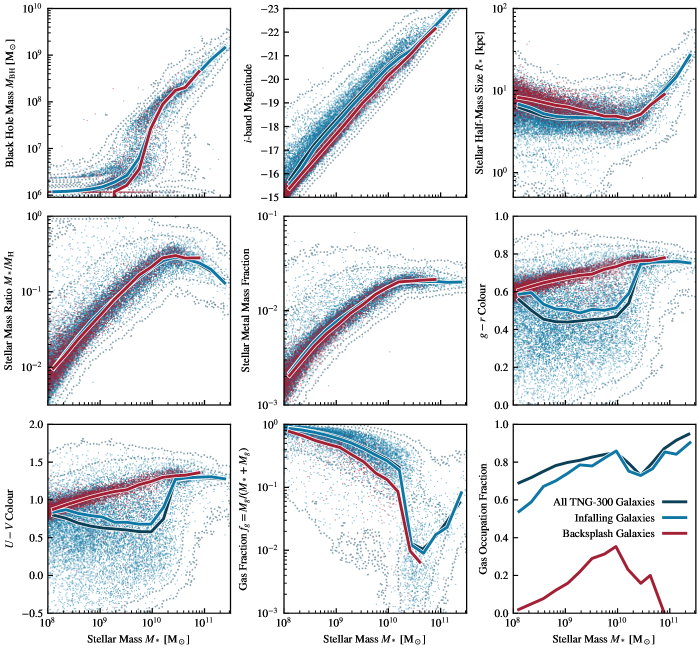
In Fig. 5 we show a number of galaxy scaling relations for the galaxies in our sample, split into three categories: backsplash (red), infalling galaxies (blue), and for comparison purposes, all galaxies in the TNG300 simulation (dark blue and background contours). Each line shows the median relation for these galaxies, binned in 16 equally log-spaced bins across the mass range shown in the figure. In the background we show scatter plots, coloured appropriately, for both the backsplash and infalling galaxies, to give some sense of scatter in the relations.

The general picture from these scaling relations is that backsplash galaxies are redder and less gas-rich than their infalling counterparts. All scaling relations are shown against the final, $z=0$, stellar mass of the galaxies (i.e. what would be observed), rather than the pre-infall mass of the galaxies. We choose to do this as we aim to classify galaxies based upon their properties, and pre-infall properties of galaxies cannot be observed. Generally, infalling galaxies are consistent with the entire TNG300 population.

In the top left panel we show the black hole mass, which is the sum of all black hole masses that are bound to the substructure. We see that, below $M_{*}\approx 2\times 10^{9}$ M_⊙, backsplash galaxies (as the median) have no black holes, but above $M_{*}\approx 10^{10}$ M_⊙ backsplash galaxies follow the same trend as infalling galaxies. We dedicate §6 to the investigation of this surprising property of backsplash galaxies in TNG300.

The top centre panel shows the $i$-band (typically the brightest out of the eight bands in the TNG catalogue) magnitude of galaxies as a function of their stellar mass. Backsplash galaxies live in a very thin band around the median, with far (0.5dex) higher (dimmer) magnitudes then their infalling counterparts, up to $M_{*}\approx 10^{10.5}$ M_⊙. This higher mass-to-light ratio for backsplash galaxies suggests that their stars are redder and older, and has been observed in prior studies (Knebe et al., 2011). At $M_{*}>10^{10.5}$ M_⊙, AGN play an important role in shutting down star formation in the galaxies, quenching them internally (rather than through external processes such as ram-pressure stripping), reducing their mass-to-light ratio (Donnari et al., 2019).

The top right panel shows the half-mass stellar size of galaxies. We see that backsplash galaxies are baised towards having higher sizes than their infalling counterparts at $M_{*}<10^{10}$ M_⊙, though there is a high degree of overlap in the two size distributions. We dedicate §5 to the investigation of size differences between backsplash and infalling galaxies.

In the centre left panel we show the stellar mass ratio $M_{*}/M_{\rm H}$, the fraction of bound mass to the galaxy that is in the stellar component. Backsplash galaxies and infalling galaxies show a similar stellar mass ratio across the mass range to their infalling counterparts, suggesting that backsplash galaxies have not preferentially lost or gained stellar mass, and that differences in their stellar properties are due to rearangement of stars and star formation either temporally (e.g. quenching) or spatially (e.g. tidal heating).

The centre panel shows the stellar metal mass fraction (frequently referred to in simulations as ‘metallicity’), which is the fraction of the stellar mass in the galaxy that is made up of elements other than hydrogen and helium. Below $M_{*}<10^{10}$ M_⊙ backsplash galaxies have a slightly (0.05–0.1 dex) lower metallicity than infalling galaxies, and have far fewer high metallicity galaxies.

The $g-r$ and $U-V$ colours of the galaxies are shown in the centre right and lower left panels, confirming the suspicions from Fig. 1 that backsplash galaxies are on average redder than infalling galaxies. The backsplash galaxies live in the well-studied red sequence of quenched galaxies, indicating that they have been quenched for a long time ($>1$ Gyr). Though there are many quenched infalling galaxies, there is a significant active population with colour $U-V\approx 0.5$. At the high mass end, $M_{*}>2\times 10^{10}$ M_⊙, we again see that the infalling galaxies become quenched (coinciding with high black hole masses, and high mass-to-light ratios in the upper panels), further indicating that AGN feedback rapidly quenches galaxies at this mass.

In the final two (lower centre and right) panels, we consider the gas fraction of the galaxies. The gas fraction,

$$f_{\rm g}=\frac{M_{\rm g}}{M_{*}+M_{\rm g}},$$ (2)

is shown for galaxies with at least one bound gas particle in the lower centre panel. Even in galaxies that retain gas, the gas fractions of backsplash galaxies are significantly lower than their infalling counterparts. Another indicator of the significance of AGN feedback can be seen at $M_{*}\approx 2\times 10^{10}$ M_⊙, where all galaxies see a sharp downturn in gas fraction thanks to the evacuating effect of these objects.

In the bottom right panel we show the gas occupation fraction of galaxies as a function of their stellar mass. The gas occupation fraction is defined as the fraction of galaxies in a bin that have a gas mass greater than zero, i.e. they contain bound gas particles. Notably, backsplash galaxies have significantly lower (3–4 times) gas occupation fractions than infalling galaxies. This staggering difference is even higher when considering clusters with $M_{\rm 200,mean}>10^{14}$ M_⊙, (not shown for brevity) where nearly all backsplashers have no gas. Such low gas occupation fractions likely originate from strong ram pressure stripping of galaxies as they pass through the cluster (Simpson et al., 2018).

4 Identifying Critical Properties

In this section, we use a decision tree classifier to identify backsplash galaxies based upon their intrinsic properties. We choose a decision tree classifier as it is highly interpretable; the outputs from the model are simply bisections in each parameter space, ranked by their importance. Through the decision tree, we can identify (in a relatively unbaised way) which features of galaxies can be used to classify them as backsplash or infalling galaxies, before moving on to the physical interpretation of these features. We note that the main reason for employing the machine learning model in this context is not necessarily to enable the use of an off-the-shelf model for using intrinsic properties to identify backsplash galaxies, as the specific normalisations of such quantities (stellar mass, black hole mass, galaxy colour, etc.) are usually not entirely converged within the simulation and modelling errors may lead to offsets to observational data (Schaye et al., 2015; Pillepich et al., 2018a). Instead, we wish to use the model to tell us which, out of all available properties, are those critical to bisecting the population of backsplashing and infalling galaxies.

4.1 Training the decision tree

Galaxy Property	Aperture	Log?
Total black hole mass	Total	$\checkmark$
Total black hole mass accretion rate	Total	$\checkmark$
Magnetic field strength in disk	Total	$\checkmark$
Magnetic field strength in halo	Total	$\checkmark$
Center of mass	Total	$\times$
Gas metal mass fractions for each species	Twice half-mass radius, half-mass radius, max radius, SF gas only	$\checkmark$
Gas total metallicity	Twice half-mass radius, half-mass radius, max radius, SF gas only	$\checkmark$
Galaxy half-mass radius (per species)	Total	$\checkmark$
Galaxy half-mass radius (total)	Total	$\checkmark$
Number of particles (per species)	Total	$\checkmark$
Number of particles (total)	Total	$\checkmark$
Total mass	Total, half-mass radius (per species, total), twice half-mass radius, max radius	$\checkmark$
Subhalo position in box	Total	$\checkmark$
Subhalo instantaneous SFR	Total, twice half-mass radius, max radius	$\checkmark$
Subhalo spin parameter $\kappa$	Total	$\checkmark$
Star metal mass fractions for each species	Twice half-mass radius, half-mass radius, max radius	$\checkmark$
Star total metallicity	Twice half-mass radius, half-mass radius, max radius, SF gas only	$\checkmark$
Magnitude in $U$, $B$, $V$, $K$, $g$, $r$, $i$, $z$ bands	Total	$\times$
Total mass within K-band half-light radius	Total	$\checkmark$
Half-light radius in K band	Total	$\checkmark$
1D velocity dispersion of all member particles	Total	$\checkmark$
Maximum value of the spherically-averaged rotation curve $V_{\rm max}$	Total	$\checkmark$
Radius at which $V_{\rm max}$ is achieved.	Total	$\checkmark$
Total mass currently decoupled as winds	Total	$\checkmark$
$U-V$ and $g-r$ colour	Total	$\times$
Cluster Property	Aperture	Log?
Group centre of mass	Total	$\times$
Group gas metal mass fractions for each species	Total	$\checkmark$
Group gas metallicity	Total	$\checkmark$
Group star metal mass fractions for each species	Total	$\checkmark$
Group star metallicity	Total	$\checkmark$
Group aperture masses	$R_{\rm 500,crit}$, $R_{\rm 500,mean}$, $R_{\rm 200,crit}$, $R_{\rm 200,mean}$, $R_{\rm 200,tophat}$	$\checkmark$
Group aperture radii	$R_{\rm 500,crit}$, $R_{\rm 500,mean}$, $R_{\rm 200,crit}$, $R_{\rm 200,mean}$, $R_{\rm 200,tophat}$	$\checkmark$

Table 1: Top: The galaxy properties used to train the decision tree. In the second column, the aperture within which this quantity is calculated is noted. Here, total refers to the total bound mass to this subhalo. In this column, half-mass radius refers to the stellar half-mass radius. Bottom: The cluster properties associated with each galaxy. These are the properties of the cluster that the galaxy has backsplashed from or is falling into. The final column for both shows whether or not the value is pre-scaled logarithmically before its use in the decision tree. Note that this does not affect results, as the decision tree simply performs a set of bisections, but it does aid in the inspection of the results.

Once we have identified all backsplash galaxies and infalling galaxies within the radius range $1<R/R_{\rm 200,mean}<2$, we assign all galaxies integer labels (zero for infalling galaxies, and one for backsplash galaxies). Alongside this, we collate all (reasonable) galaxy properties from the publicly available TNG SubFind catalogues. These are shown in Table 1, with the properties of their hosts that are also included in their description. Finally, we include the current distance between the galaxy and cluster centre, $R_{\rm gal}$ in units of the cluster $R_{\rm 200,mean}$. Most properties are logarithmically scaled ($R_{\rm gal}$ is not), as this eases in the interpreation of the results from a physical standpoint. As the decision tree framework does not accept any values that are infinity or not a number, we bound all scaled values as a lower limit of -10. Typically when a property has a physical value of zero (and hence logarithm of -inf), the decision tree uses a cut to check for occupation of this value (e.g. gas mass), so the specific value chosen here does not impact our results.

The results in this section are based upon the clusters with mass $10^{14}<M_{\rm 200,mean}/{\rm M}_{\odot}<10^{15}$, to reduce complexities associated with cluster evolution but to still leave a large sample of clusters (215) and backsplash galaxies. Additionally, we make a cut in galaxy stellar mass $M_{*}>10^{8}$ M_⊙ (10 particles), mainly to ensure that there are enough particles such that the occupation of the subhalo is accurate. At low masses, where there are only one or two particles in a subhalo, there may be many similar subhaloes that are unoccupied simply by chance, as star formation in the TNG model is a stochastic process (Genel et al., 2019; Keller et al., 2019).

To train the decision tree, we transform all associated features ($N_{\rm feat}$) with the $N_{\rm gal}$ galaxies into a $N_{\rm feat}\times N_{\rm gal}$ matrix, with an associated one dimensional array containing the integer labels. These two arrays are then shuffled, to simplify training and validation splits.

We leverage the decision tree classifier object already implemented in the python package Scikit-Learn (Pedregosa et al., 2011). When training, we use the Gini impurity for the split criterion, the “best” split strategy, a maximum tree depth of 6, and a minimal impurity decrease of 0.001. Choosing instead to use the entropy information gain criterion, or larger tree depths, do not qualitatively change our results. We choose the depth and minimum impurity decrease to make the tree easier to visually inspect, and for performance reasons.

To investigate the accuracy of our model, we use a 80–20 validation and training split. Our decision tree gets a 20% cross-validation score of 89%, meaning that when trained on a 80% of the data, and tested on 20%, we are able to correctly predict the classification of a galaxy 89% of the time. However, as we are mainly interested in the ability of the model to predict whether or not something is a backsplasher, rather than the ability of the model to predict if a galaxy is infalling, we now focus on our positivity and false positive rate. When considering only galaxies that are backsplashers, we have a 20% positivity rate of 78%, meaning that we mis-classify 22% of backsplash galaxies as infalling galaxies. However, we only have a 7% false-positive rate, meaning only 7% of the galaxies predicted by the model to be backsplash galaxies are actually infalling. The accuracy of our decision tree model is comparable to other recent studies that additionally employ phase-space information, with Farid et al. (2022) able to achieve an 83% classification accuracy when using phase-space information and sSFR with a random forest model. The hard classification model in Farid et al. (2022) is designed to separate infalling galaxies and those within the cluster, however, and does not explicitly classify backsplashers. Their hard classification model cannot accurately predict the existence of bound structures to the cluster in the range $R>R_{\rm 200,mean}$.

Such a high level of accuracy is surprising given the large level of overlap between the backsplash and infalling population (see Fig. 5). For instance, making a cut based on simple population statistics, with $R/R_{\rm 200,mean}<1.2$, and a red sequence cut in $g-r$ magnitude, returns a positivity rate of under 30% (though with only a 3% false-positive rate owing to the markedly lower number of galaxies classified as backsplashers).

4.2 Interpreting the model

Figure 6: Gini importances of the top ten highest ranked features in the TNG300 datasets, when classifying backsplash galaxies. A higher importance score corresponds to a higher level of information gain when bisecting this property. Descriptions of the symbols used here are available in the text.

Figure 7: The highest ranked features from Fig. 6 scattered against each other. The bottom left triangle shows all galaxies in the sample, with blue points representing infalling galaxies and red points representing backsplash galaxies. The dashed lines show the cuts identified by the decision tree based on the top five most important features, with the top right panels showing the resulting parameter space after the cuts have been applied to find the largest contiguous volume of backsplash galaxies. This time, the blue points are plotted on top of the red points to highlight false positive detections. In this region, we find 603 backsplash galaxies with a false-positive rate of 15%.

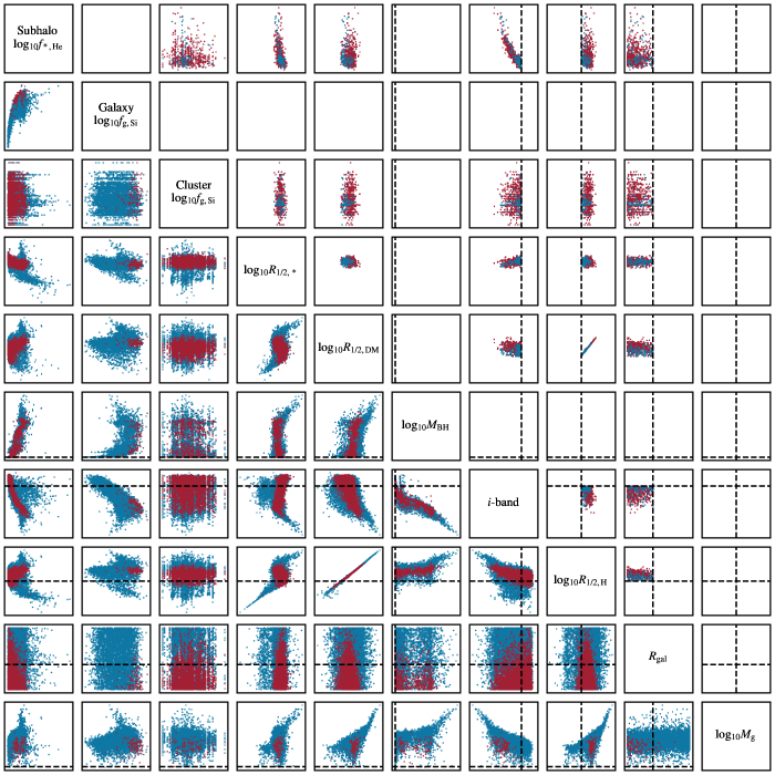
That we can classify galaxies as backsplashers from their intrinsic properties without detailed kinematic information is interesting, but not as interesting as answering why we can classify them. Fig. 6 shows the feature (Gini) importances for the top ten features in the model for bisecting the infalling and backsplash galaxy populations. Their correlations are also shown in Fig. 7, where backsplash galaxies are shown in red, and infalling galaxies in blue. In this figure, dashed black lines show the bisections that the decision tree predicts are the most likely to segment the two populations, with the series of cuts in the tree shown for the leaf node with the highest number of backsplash galaxies. The top right panels show the same projections but with the cuts applied to the whole population.

The most important feature in the entire model is $\log_{10}M_{g}$, the gas mass of the galaxy. We can see that this feature is used for occupation testing by the model, with the majority of backsplash galaxies (see the bottom right panel of Fig. 5) containing zero gas. This is even more stark when applied to the more massive clusters, with gas occupation fractions of backsplash galaxies reducing as the clusters get more massive due to increased ram pressure stripping.

For the second most important feature, it is fair to say that the decision tree has ‘learned’ about the geometry of the problem (Fig. 3), with the liklehood of a galaxy being a backsplasher dropping rapidly with distance from the cluster centre. The decision tree places a cut when just over 50% of the galaxies are likely to be infalling ($R_{\rm gal}/R_{\rm 200,mean}=1.41$). This is clear to see as well in Fig. 7, where the frequency of backsplash galaxies clearly drops off with increasing $R_{\rm gal}$.

Next, there are three measures of galaxy size. In decreasing order of importance, the model finds that $\log_{10}R_{\rm 1/2,H}$ (total bound half-mass radius), $\log_{10}R_{\rm 1/2,DM}$ (dark matter half-mass radius), and $\log_{10}R_{\rm 1/2,*}$ (stellar half-mass radius) are useful indicators of backsplash status. As this topic is somewhat complex, we dedicate an entire section of the paper to it (§5), but briefly we see that backsplash galaxies tend to have larger stellar half-mass sizes, and larger (or smaller) dark matter half-mass sizes for higher mass (lower mass), than their infalling counterparts.

The model finds that a cut in $i$-band magnitude is useful in segmenting the two populations, but it chooses a very low luminosity cut (with $i<-16.7$). In Fig. 5, we see that at these low magnitudes the overlap between the infalling and backsplash populations becomes higher, making segmenting them based upon this property troublesome. Although the prescence of this cut is useful, it is likely to be more numerically motivated, as at this luminosity (and hence mass) photometry is not particularly well resolved, with the star formation history of the galaxy being traced by around 10 stellar particles. With increasing resolution, the turn down of the $i/\log M_{*}$ relation seen in Fig. 5 at the lowest luminosities would likely disappear, but it is notable that the model picks up numerical differences between populations, as well as physical differences, indiscriminately.

In a similar fashion to the gas mass of galaxies, the model uses the black hole mass as an occupation check, with it placing a cut in the black hole mass $\log_{10}M_{\rm BH}$ below the seed mass of black holes in the simulation. This is why in the top right of Fig. 7, the black hole mass panels contain zero points; the model has selected only galaxies that currently have zero black hole mass. As with the sizes, we dedicate a section (§6) to the investigation of this.

Finally, the model finds that some species fractions contribute to the ability to bisect the two populations. First, the cluster silicon gas fraction ($\log_{10}f_{\rm g,Si}$), which is the mean silicon gas fraction within all gas particles bound to the cluster associated with the galaxies. Secondly, we find that, in galaxies that retain their gas, their gas silicon abundance is a useful criterion to bisect on. Finally, the fraction of galaxy stellar mass that is helium ($\log_{10}f_{\rm*,He}$) contributes to the ability to bisect the two populations. Vogelsberger et al. (2018) and Barnes et al. (2018) investigated clusters in the TNG300 simulation, and showed that cool-core clusters, with relaxed morphologies, have significantly higher levels of enrichment in their cores. This may suggest that higher cluster enrichment levels may correlate with different tidal interactions between galaxies and the cluster, but we see no significant correlation between $\log_{10}R_{\rm 1/2,DM}$ and $\log_{10}f_{\rm g,Si}$ in Fig. 7. It is additionally clear that further cuts on the cluster silicon abundance and galaxy helium abundance would be able to separate out a cleaner sample of backsplash galaxies, but along with the low importance indicated by the decision tree it is likely that this is simply by chance.

5 Understanding Galaxy Sizes

In Fig. 6, we saw that some of the leading-order features separating backsplash and infalling galaxies were there sizes in various mass types (total mass, dark matter mass, and stellar mass). These splits were used downstream of the occupation cut in gas mass, with star formation rates in the halo catalogues computed instantaneously from the bound gas (and hence all of the backsplash galaxies were passive). This means that these features are useful irrespective of active/passive status of galaxies as seen by the model.

Figure 8: Mass-size relations for backsplash galaxies (red) and infalling galaxies split into quenched (dark green) and active (light green) populations by specific star formation rate ${\rm sSFR}=10^{-11}$ year^-1. In the background the scatter shows all galaxies in the sample, with the solid lines representing the median in 16 equally log-spaced bins, and dashed lines showing the 16–84 percentile range. The top panel shows the stellar half-mass radius, and the bottom panel shows the dark matter half-mass radius. The dotted vertical line shows the total bound mass at which AGN feedback becomes significant, leading to a noticeable up-tick in the stellar sizes. The numbers in the top left of the bottom panel show how many galaxies are in each cut below the point at which AGN feedback becomes significant.

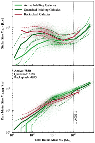
In Fig. 8 we show the relationship between total bound mass of galaxies and their stellar and dark matter half-mass sizes (top and bottom panels respectively). These relationships are split by their active and passive nature for infalling galaxies, with backsplash galaxies grouped together (the quenched fraction of backsplash galaxies is 94% so splitting these makes little sense). Here, we take the active/passive threshold to be a specific star formation rate ${\rm sSFR}={\rm SFR}/M_{*}=10^{-11}$ year^-1, computed from the instantaneous gas star formation rate. Only galaxies with at least $M_{*}>10^{8}$ M_⊙ are included in this analysis, but all clusters are included.

As in Genel et al. (2018), we find that quenched galaxies have significantly larger stellar sizes than their active counterparts. At the lowest masses ($M_{\rm H}<10^{11}$ M_⊙), backsplash galaxies show even larger stellar sizes than their quenched counterparts.

In Genel et al. (2018) one of the main explanations for low-mass galaxies being large is that they have experienced significant tidal heating, as the sample of low mass galaxies are almost entirely satellites. Here, we are able to show that ‘field’ galaxies (in this context, these are galaxies that have not been processed by the cluster yet, so infalling galaxies) that are quenched have experienced similar size growth at low masses as the general quenched population, suggesting a different explanation is warranted.

At the high-mass end of the stellar sizes, we see that backsplash galaxies grow their sizes faster (at lower masses) than infalling galaxies, but there are few backsplash galaxies of this mass and as such this result is tenuous. At the highest masses, $M_{\rm H}>10^{12}$ M_⊙, quenched and active galaxies have similar sizes when separated by instantaneous specific star formation rate. This similarity is likely due to the method of quenching; these galaxies are mainly quenched by their central AGN periodically, going through phases of feedback and gas evacuation, followed by fresh accretion and cooling leading to increases in star formation. Here the quenched and active separations only show different epochs of the evolution of these galaxies.

The dark matter sizes of galaxies are generally more similar, with a notable kink in the infalling galaxy sizes at $M_{\rm H}=10^{11}$ M_⊙ that is not present in the backsplash galaxies. This kink is likely caused by the introduction of black holes to the haloes, which occurs at total FoF halo masses of $7.4\times 10^{10}$ M_⊙ in the TNG model, with AGN feedback having been shown to decrease the central density of dark matter in simulations (Duffy et al., 2010).

At masses below the kink, backsplash galaxies are the largest, but this trend is reversed after the kink where they are the smallest. This indicates that at low masses, similar processes are governing the size differences (i.e. low mass galaxies have large stellar and dark matter sizes for the same reason) but at higher masses the stellar component and dark matter components are affected by different processes. In addition, at masses below $M_{\rm H}<10^{11}$ M_⊙, stellar and dark matter half-mass sizes are comparable, of order 10 kpc. At higher masses, the dark matter half-mass size is significantly larger, breaking the scales between the dark matter and stellar components.

Figure 9: The two galaxy size measures from Fig. 8 shown against each other, with the same line styles and colours. In the background we show the 1:1 relation as a thick dotted black line, and for comparison purposes show the physical softening length at $z=0$ in the TNG300 simulation of 1.48 kpc as a dot-dash grey line. We show, similarly to Genel et al. (2018), that quenched galaxies show larger stellar sizes on average even for a fixed halo size. The thin background dotted grey lines show the scale of $2.8\epsilon$, the characteristic scale identified in Campbell et al. (2017) at which sizes begin to flatten.

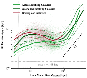
In Fig. 9 we show the two measures of galaxy size against each other, alongside the softening scale. Campbell et al. (2017) found that galaxy stellar sizes flatten at a charachteristic scale (2.8 times the softening length $\epsilon_{\rm DM,*}$, which for TNG300 is 1.48 kpc at redshift $z=0$), and this appears to be true within TNG300, also. However, whilst the active galaxy sizes saturate at around 4.2 kpc, as predicted by Campbell et al. (2017), our quenched galaxy sizes (and backsplash sizes) rise above this level for the lowest masses. As TNG300 haloes and galaxies grow, they begin to revert to the 1:1 relation (at dark matter sizes above 100 kpc).

Ludlow et al. (2019a), Ludlow et al. (2019b), and Ludlow et al. (2020) discuss origins of this potentially spurious size growth in galaxies, and suggest that its origins lie in 2-body scattering between different particle species (in this case, dark matter and stars) with different masses. In this scenario, energy is transferred from the more massive component (dark matter) to the less massive component (stars), causing the dark matter to be centrally concentrated within the halo and the stellar component to be dynamically spread. Galaxies that are artificially inflated by 2-body scattering are then expected to have more massive, cuspier, inner dark matter profiles, and hence smaller dark matter sizes at a given mass.

Our relationship between $R_{\rm 1/2,DM}$ and $R_{\rm 1/2,*}$ is generally flat at dark matter sizes below 100 kpc (i.e. it does not continue down the 1:1 relation), indicating that sizes are propped up in this case by softening inflation, with a minimal stellar (and dark matter) size set by $2.8\epsilon\approx 4.5$ kpc. There is clearly more to this, however, with there being significant differences between active and passive infalling galaxies, as well as the backsplash population.

In TNG-50, where significantly higher resolution simulations are available (a rough factor of 100 smaller particle masses), Pillepich et al. (2019) showed that at the resolution of TNG300, (roughly TNG-50-3) the stellar half-mass sizes of galaxies were not converged below $M_{*}<10^{9.5}$ M_⊙. Higher resolution generally gives smaller stellar sizes, consistent with the indications of Ludlow et al. (2021) that this may be due to lower levels of dynamical heating due to the lower dark matter masses used, or that the sizes are inflated due to oversoftening (as the chosen softening frequently scales with resolution). It is hence likely that 2-body scattering, as well as size inflation caused by softening, cause a systematic trend in our galaxy sizes at low masses ($M_{*}<10^{9.5}$ M_⊙) to become larger, meaning that the absolute sizes of our low-mass galaxies are overestimated. This does not mean, however, that any differences between the galaxy populations on these scales are entirely numerically driven. In particular, that we see differences in dark matter sizes at $M_{\rm H}<10^{11}$ M_⊙ is reliable, as these sizes are both much larger than the softening scale (see Fig. 9) and generally would be made smaller, not larger, by 2-body scattering.

Figure 10: Mean stellar density profiles, split by final stellar mass (panels). Solid lines show the median, with the dashed lines showing the 16–84 percentile range, of 1024 mean-stacked bootstraps (with replacement) of all individual profiles. The vertical grey dot-dash line shows the gravitational softening used for stellar and dark matter particles, and the dotted lines show the median stellar half-mass radius for galaxies in each mass bin of the corresponding colour. In the background the lighter, thinner, line show the dark matter density profile, multiplied by 0.1 for clarity.

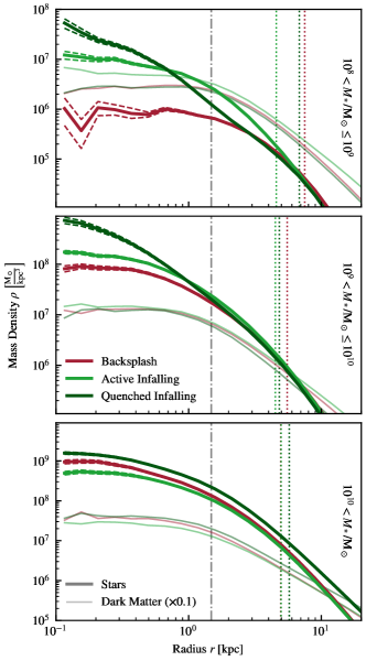
In Fig. 10 we show the mean-stacked stellar mass and dark matter mass profiles for the inner 20 kpc of all galaxies within each mass range. These profiles include all bound matter, and are stacked for three different mass ranges: $10^{8}<M_{*}/{\rm M}_{\odot}\leq 10^{9}$, $10^{9}<M_{*}/{\rm M}_{\odot}\leq 10^{10}$, and galaxies above $M_{*}>10^{10}$ M_⊙. The lines show the mean density, stacked across all galaxies in the mass range, with the final calculated mean the median of 1024 bootstraps (with replacement) of the original selection. The bootstrapping is used to estimate the error on the mean density, with the 16–84 percentile range shown as dashed lines. We also show the dark matter profiles of the same galaxies, stacked in the same way, as lighter lines in the background.

Fig. 10 shows that backsplash galaxies have a significantly lower central stellar density than their infalling counterparts of the same mass. They also show a much more centrally concentrated density profile, in contrast to the quenched infalling galaxies which have a strong cusp in the central stellar density. These differences in stellar profiles are despite the dark matter profiles of the two classes of galaxies being extremely similar.

As in each cut the masses of the galaxies are constrained to be similar, we can see that although the sizes of the quenched infalling galaxies and backsplash galaxies are similar, these originate through very different distributions. The quenched galaxies have a much steeper profile that drops off rapidly, whereas the backsplash galaxies have a shallower profile that catches up and overtakes the quenched profile at large radii.

The flat central profiles of the backsplash galaxies are consistent with those seen in Carleton et al. (2019), where the central stellar core is tidally heated through close interactions with the cluster halo as the galaxies orbit. Tidal heating injects energy into particles within the galaxy as it falls into a cluster on a (crucially) eccentric orbit, with the shear forces on the bound particles changing rapidly with time. Tidal heating of backsplash galaxies is further consistent with the increased sphericity seen in the shapes of backsplash galaxies in prior works (Knebe et al., 2020).

Such tidal interactions have been suggested to be the origins of ultra-diffuse galaxies. A number of authors (e.g. Benavides et al., 2021; Trujillo, 2021) have recently suggested that tidal heating and stripping processes could play a role in forming such UDGs. The suppression of the central stellar density of the backsplash galaxies identified in this study certainly make them UDG candidates, and further suggest that a large number of UDGs near clusters may well be backsplash galaxies. We caution, however, that the suppression of the central stellar density occurs close to the softening scale of the TNG300 simulation, making the close gravitational interactions less accurate than would be ideal for studying such complex dynamics. These results suggest that follow-up studies should focus on these low-mass backsplash galaxies, as they are potentially the most distinct from their infalling counterparts, but due to the limited resolution of TNG300 we are unable to make direct comparisons to nature.

Figure 11: Mean total density profiles, split by final bound mass ($M_{\rm H}$; panels). Solid lines show the median, with the dashed lines showing the 16–84 percentile range, of 1024 mean-stacked bootstraps (with replacement) of all individual profiles. The dotted lines show the median bound mass half-mass radius for galaxies in each mass bin of the corresponding colour. Note that the horizontal range is shifted significantly from the same figure for the stellar component (Fig. 10). The inner regions are not shown as the profiles of all cuts are all consistent in dark matter and deviations are powered by differences in the stellar component.

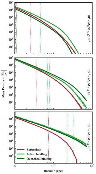
In Fig. 11 we show the outer (total mass, though in this region the mass density is dominated entirely by dark matter) profiles of our haloes. Here, we split by halo mass, but only include galaxies that are occupied by at least $M_{*}>10^{8}$ M_⊙ for consistency. We see that at masses $M_{\rm H}>10^{10}$ M_⊙ there is significant disruption of the backsplash subhaloes, leading to smaller dark matter half-mass sizes (as can be seen in Fig. 10, the inner dark matter profiles are consistent for backsplash and infalling galaxies). This suggests that there has been significant tidal stripping of subhaloes as they have passed through the cluster, with the strength of the stripping increasing with increasing subhalo mass. This is consistent with the results from Jiang & van den Bosch (2016) who studied the disruption of subhaloes in the Bolshoi simulation, and found that the tidal mass loss rate, $\mathrm{d}M_{\rm H}/\mathrm{d}t\propto M_{\rm H}^{1.07}$, shows superlinear growth with subhalo mass.

van den Bosch (2017), van den Bosch et al. (2018), and van den Bosch & Ogiya (2018) all discuss the potential origins of forces leading to tidal stripping, and whether the disruption of substructure is numerical or physical in nature. Notably, they find that disruption of subhaloes is converged over many softening scales and resolutions on short timescales (comparable to one or two cluster crossing times, see Fig. 10 in van den Bosch & Ogiya (2018)), but subhaloes continue to lose mass due to numerical effects on long timescales. van den Bosch & Ogiya (2018) focused only on subhaloes on small ($R/R_{\rm vir}\approx 0.15$) circular orbits, however, meaning that in realistic scenarios (like our backsplash subhaloes), the weaker tidal fields may have a less significant effect. As our backsplash galaxies are typically on their way to their first periapsis (i.e. they have only been influenced by the cluster for a relatively short amount of time), we suggest that the tidal disruption that our subhaloes have experienced is likely to be physical at large radii.

In summary, we have found that the stellar sizes of backsplash galaxies are larger than the general field population, especially at low masses, whilst the bound mass (or dark matter mass) sizes of these galaxies are smaller than the field population, for a given subhalo or stellar mass. We have discussed how these differing sizes are likely due to tidal interactions with the host cluster: as galaxies fall in to the cluster, their cores ($r<5$ kpc) are tidally heated (leading to a flatter inner stellar density profile, and larger stellar size, see Fig. 10), whilst their extremities ($r>100$ kpc) are tidally stripped (see Fig. 11). This leaves us with galaxies that are dark matter dense, but gas and star poor, making the backsplashing of galaxies a potential UDG formatiom mechanism, as suggested by prior authors.

6 Black Hole Occupation

Figure 12: Tracks of cluster galaxies, rescaled to ensure that their pericentres overlap in time, all falling into the same ($M_{\rm 200,mean}=2.13\times 10^{15}$ M_⊙ cluster). Each line (different colours) shows a different infalling galaxy). From top to bottom, the panels show the orbital radius of the galaxies, their stellar and dark matter half-mass radii, their bound stellar mass within twice the (stellar) half-mass radius, their bound gas mass (note when lines leave the bottom of the plot they have a value of zero) in the same aperture, and the total bound black hole mass, as a function of time.

To better understand both the radial profile differences explored in §5, and the importance of the black hole mass in classifying backsplash galaxies, we now consider the evolution of individual backsplash galaxies.

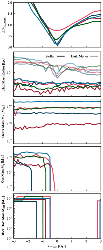
In Fig. 12 we show the properties of backsplash galaxies falling into the most massive cluster in the volume ($M_{\rm 200,mean}=2.13\times 10^{15}$ M_⊙ cluster). These five galaxies are selected randomly through the mass range, and are chosen to have one pericentre before residing outside of the cluster at $z=0$.

In the top panel of Fig. 12 we show the radial tracks of the galaxies as they fall into, and rebound from, the cluster. To ensure that we can consistently compare the galaxies, we re-scale the time axis by the time at which each galaxy reaches the pericentre of their orbit $t_{\rm peri}$. This time is computed as the output time of the snapshot at which the radius $R(t)/R_{\rm 200,mean}(t)$ is at a minimum. We see that there are some galaxies present that only have a glancing orbit (pink curve) and some that have pericentres very close to the centre of the cluster, such as the dark and light blue curves.

The second panel of Fig. 12 shows the half-mass sizes for stars (dark) and dark matter (light). We see that as low mass galaxies (red and green) pass pericentre, their stellar sizes are inflated, and all galaxies have their dark matter half-mass sizes reduced during their time in the cluster. This further strengthens our hypothesis from §5 that tidal interactions with the cluster control these two variables.

The third panel in Fig. 12 shows the stellar masses of the galaxies over time, here showing the stellar mass within twice the half-mass radius. That there is little evolution in this quantity over time, even at pericentre passage, suggests that rather than explicitly losing mass to produce a more cored stellar profile (Fig. 10) the stellar mass in the centres of the galaxies is simply rearranged, strengthening our hypothesis that this rearrangement occurs due to tidal heating.

In the fourth panel, we show the gas mass within twice the stellar half-mass radius for each of the galaxies. We see that by the time that the galaxies have reached the pericentre of their orbit they have all lost all of their gas through ram pressure stripping from the cluster. This even occurs in the galaxy with a relatively shallow orbit (pink curve, $R_{\rm peri}\approx 0.8R_{\rm 200,mean}$), suggesting that ram pressure stripping is very efficient in this massive cluster. In idealised simulations of galaxies in ‘wind tunnels’, Tonnesen & Bryan (2009) found that galaxies are stripped of over half of their gas mass in under 0.5 Gyr upon entry into a cluster-like environment. Simpson et al. (2018) studied backsplash galaxies (dwarfs orbiting local groups) in simulations, and found that even in these shallow potentials satellites can be completely stripped of gas.

Finally, in the bottom panel, we show the black hole mass of the galaxies as a function of their orbital time. On a similar timescale to their gas loss, the cluster galaxies appear to lose their black holes. This is unexpected, as the black holes act as collisionless particles and typically reside in the centres of the cluster galaxies which we have seen in the second panel ($M_{*}$) are relatively protected aside from tidal heating. Further, black hole particles are ‘pinned’ to the centres of their galaxies by a ‘repositioning’ scheme that attempts to insulate them from spurious numerical heating (see Weinberger et al., 2017, Section 2.2). In addition, we see that once the galaxies have moved away from the cluster (at $t-t_{\rm peri}>2.5$ Gyr) they appear to re-grow black holes, but at larger masses than the black hole seed mass in the simulation ($1.1\times 10^{6}$ M_⊙, see Pillepich et al., 2018a).

Figure 13: A schematic showing the stripping of black holes from their host backsplash (or cluster) galaxies. The dark red line shows the path of the backsplash galaxy, in the reference frame of the black hole at the centre of the central brightest cluster galaxy (BCG, black circle). The green line shows the original black hole associated with the backsplash galaxy, which is removed by the repositioning scheme once the galaxy is stripped of all of its gas. Once back outside the cluster, the backsplash galaxy is re-seeded with a new black hole (pink line), before residing outside the cluster at $z=0$.

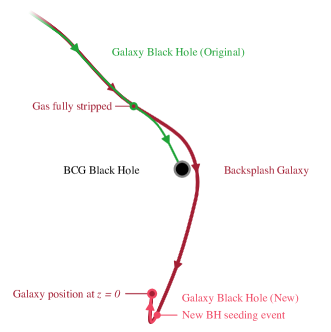
It appears in this case that the repositioning scheme, initially intended to ensure that the positions of black holes remained stable, is the downfall of black holes living within cluster galaxies. The black hole repositioning scheme is designed to ensure that the particle is repositioned onto the particle (of the nearest 1000) with the lowest gravitational potential. When repositioned, the black hole particle is given the same velocity relative to the volume as the particle it is repositioned onto. If the galaxy is a central, e.g. the brightest cluster galaxy (BCG), then such a scheme keeps the black hole pinned to the potential minimum. In a cluster galaxy that is undergoing stripping, however, this leads to the black hole being repositioned onto either a particle with a high relative velocity to the halo, or a member bound to, and phase mixed with, the cluster, making it leave the substructure. This eventually leads to the rapid movement of the black hole to the centre of the cluster, merging with the black hole at the centre of the BCG. Fig. 13 shows a schematic, based upon the path of the light blue trace in Fig. 12, of how a black hole is lost and re-seeded in a backsplash galaxy.

Figure 14: Shows the occupation fraction of black holes, computed as the number of galaxies in this bin that have a black hole divided by the total number of galaxies, for 16 equally log-spaced bins between the figure limits. Each line shows a different aperture around the cluster within which the occupation fraction is computed. The occupation fractions here are shown for the most massive cluster in the volume, and the same cluster shown in Fig. 12, with $M_{\rm 200,mean}=2.13\times 10^{15}$ M_⊙, though these trends occur across the mass range.

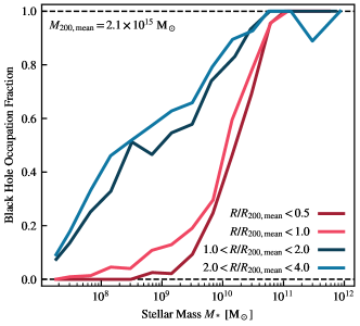
Fig. 14 shows the occupation fraction of black holes as a function of their stellar mass, in various apertures. The blue lines show apertures generally containing field and infalling galaxies, with the red lines showing the cluster galaxy component. Notably, the occupation fraction of galaxies within the cluster is significantly lower, especially at lower masses (those expected to survive post-apocentre to become backsplash galaxies). Below $M_{*}<10^{10}$ M_⊙, galaxies within the core of the cluster ($R/R_{\rm 200,mean}<0.5$) have occupation fractions that are roughly zero, suggesting all of these (there are 1243 galaxies with $10^{7}<M_{*}/{\rm M}_{\odot}<10^{10}$) galaxies have lost their black holes. The higher mass galaxies are those less likely to become backsplashers, as they generally rapidly merge with the central due to dynamical friction (Bakels et al., 2021), and as such are less likely to have already had their pericentre and lost their black hole.

Recent works, such as Bahé et al. (2021), have noted that there appears to be a lower than expected black hole occupation fraction for cluster galaxies (see their Appendix A). Notably, the model discussed in Bahé et al. (2021) also repositions only on gas particles, as typically the neighbour-finding structures (e.g. trees) within N-body codes are only set up to include gas particles for optimisation reasons. Our results, along with those in Bahé et al. (2021), suggest that the black hole occupation fraction of cluster galaxies is severely underestimated within cosmological simulations that employ such repositioning schemes.

Such issues with the repositioning of black holes are likely to persist amongst many of the state-of-the-art large-volume simulations, including the entire Illustris and IllustrisTNG suite, as well as the EAGLE suite and derivatives (Vogelsberger et al., 2014a; Schaye et al., 2015). Simulations that do not employ repositioning, such as the Horizon-AGN suite (Dubois et al., 2012), or Romulus (Tremmel et al., 2017), will not suffer from this artificial stripping of black holes from cluster galaxies. Prior work from Ragone-Figueroa et al. (2013) employed repositioning on all particle types, though unlike TNG has black hole growth dominated by accretion at all masses (Bassini et al., 2019), with TNG black holes showing merger-dominated growth at $M_{\rm BH}>10^{8}$ M_⊙ (Weinberger et al., 2018). It is possible that these authors, like the EAGLE simulations, included a maximal velocity difference between the black hole and repositioning candidates, but a full investigation of the implementation of black hole recentreing strategies is out of the scope of this work. Additionally, modifying the neighbour finding structures used for repositioning to employ stellar particles for recentreing purposes would insulate such schemes from these effects. The SIMBA simulation suite, that employs a loop over nearby stellar particles to compute accretion rates, already uses a recentreing prescription that includes the use of stellar particles, and likely does not suffer from these black hole stripping issues (Anglés-Alcázar et al., 2017).

Haidar et al. (2022) investigated the occupation fraction of black holes in a number of cosmological simulations, and found that the SIMBA suite, that repositions on stars as well as gas particles, have occupation fractions of close to 100% even down to low masses. They find that EAGLE and IllustrisTNG actually reduce their global occupation fractions of low-mass galaxies over time, due to the increasing fraction of galaxies resident in clusters. We have now demonstrated the specific numerical pathway through which these galaxies are stripped of their black holes.

There are a number of potential pitfalls for galaxy formation simulations with black hole stripping. Primarily, aside from the black hole occupation fractions being clearly incorrect (the artificial seeding procedure makes these numbers uncertain anyway), the contribution to the cluster energy budget from the AGN resident in cluster galaxies will be underestimated. Additionally, the merger rates of black holes, particularly those in the centres of clusters, will be overestimated, as will their masses. The impacts of these outcomes are not yet known, but as black hole seeding and AGN models are explicitly calibrated against observational data (e.g. Crain et al., 2015; Pillepich et al., 2018a) and as such these potential pitfalls may already be calibrated into the choice of free parameters.

7 Conclusions

Backsplash galaxies are galaxies that have previously had a pericentre within the bounds of a galaxy cluster, but have since migrated outside of most typical definitions of the cluster boundary. Their intrinsic properites are not well understood, as simulating such galaxies is numerically challenging due to the high inherent dynamic range of masses and spatial scales present in galaxy clusters.

In this paper we have explored the properties of backsplash galaxies in the TNG300 simulation by tracing the orbits of galaxies with stellar mass $M_{*}>10^{8}$ M_⊙ within $1<R/R_{\rm 200,mean}<10$ of our 1302 isolated clusters with $M_{\rm 200,mean}>10^{13}$ M_⊙. By classifying galaxies into ‘backsplash’ and ‘infalling’ categories based upon whether the galaxy has previously been within $R_{\rm 200,mean}$ of the cluster re, we were able to find that:

• The abundance of backsplash galaxies grows roughly linearly as a function of galaxy cluster mass, with $M_{\rm 200,mean}\approx 10^{14}$ M_⊙ clusters on average hosting around 5 backsplashers, and clusters with $M_{\rm 200,mean}\approx 10^{15}$ M_⊙ hosting around 50 on average. Backsplash galaxies are significantly more common (relative to infalling galaxies) at smaller radii, with equipartition reached between the two populations at $R=1.24R_{\rm 200,mean}$. These two results suggest that observations targeting backsplash galaxies should focus on the intermediate regions ($1<R/R_{\rm 200,mean}<1.5$) of the highest mass clusters $M_{\rm 200,mean}>10^{14.5}$ M_⊙, to reduce contamination and ensure adequate sampling.

• We verify that backsplash galaxies and infalling galaxies are kinematically separated, with the separation increasing as a function of host cluster mass. Both backsplash and infalling galaxies have a roughly gaussian radial velocity ($v_{\rm r}$) distribution, with infalling galaxies having a mean velocity $\bar{v}_{\rm r}<0$ dependent on cluster mass ($\bar{v}_{\rm r}=-1100$ km s^-1 for $M_{\rm 200,mean}\approx 10^{15}$ M_⊙). Backsplash galaxies have a typical mean radial velocity of $\bar{v}_{\rm r}\approx 0$, with the width of the distribution dependent on cluster mass. These findings confirm that the use of phase-space information is an excellent way to classify backsplash galaxies, if it is available (e.g. as in Farid et al., 2022).

• By considering typical galaxy scaling relations, we have shown that backsplash galaxies in TNG300 are typically black hole-poor, have higher mass-to-light ratios, larger stellar sizes, redder colours, and lower gas fractions than their infalling counterparts of a similar stellar mass. These characteristics are generally consistent with galaxies that have been ram pressure stripped, quenched, and tidally heated, processes thought to be common in galaxy clusters, and that have previously been shown to impact the evolution of backsplash galaxies (e.g. Simpson et al., 2018).

• To investigate which intrinsic properties of galaxies (without considering phase-space information) are key to separating the infalling and backsplashing population we trained a decision tree classifier on all available (reasonable) properties from the TNG SubFind catalogues of our two populations. The classifier identified the most important features in separating the two populations of galaxies as the galaxy gas mass, distance from the cluster re, galaxy and halo size, magnitude, and black hole mass. Our decision tree classifier was able to classify backsplash and infall galaxies with high accuracy, returning a 20% cross-validation score of 89%. When considering backsplash galaxies alone, the classifier had a low (7%) false-positive rate, and a relatively low false-negative rate (22%). These levels of accuracy are comparable with other hard classifiers that do employ phase-space information, such as those used recently by Farid et al. (2022). Despite the high accuracy of the classifier, however, it would be impractical to use for observations, and as such we simply use the decision tree as a way to reduce the extreme dimensionality of our feature space, finding interesting galaxy properties to focus follow-up analysis on.

• Through the analyis of galaxy sizes and profiles, motivated by the decision tree, we showed that backsplash galaxies have typically larger stellar sizes at low mass, and smaller dark matter sizes at high mass, than their infalling counterparts, even when accounting for the size growth of quenched galaxies due to numerical effects (Genel et al., 2018). We discussed how, despite numerical concerns with (relatively) low resolution simulations like TNG300, our results still suggest that the central regions of backsplash galaxies are tidally heated, leading to flatter stellar inner density profiles. They also suggest that backsplash galaxies are subject to tidal stripping, with the outskirts of backsplash galaxies relatively devoid of dark matter relative to their infalling counterparts. We discussed how these processes contribute to the potential formation of UDGs near clusters, where UDGs are likely to be backsplash galaxies.

• We investigated the low black hole occupation fraction of backsplash galaxies by tracking the detailed properties of individual galaxies back over time. We showed that backsplash galaxies typically lose all of their gas mass before reaching the pericentre of their orbit around the cluster, even when their orbit is shallow. We also showed how the black hole repositioning (or re-reing) prescription, which moves black hole particles within galaxies based on the local potential sampled by gas particles, leads to the extraction of black holes from infalling galaxies as they near the pericentre of their orbit. Such repositioning schemes, required to insulate black holes from spurious heating out of central galaxies and to maintain the efficiency of AGN feedback, hence come at the cost of underestimating the occupation fraction of black holes in cluster galaxies and hence their feedback contribution within clusters.

The large sample size of isolated massive haloes ($M_{\rm 200,mean}>10^{13}$ M_⊙) in TNG300 has enabled us to study a representative sample (over 5000) of backsplash galaxies. We have found that the properties of these galaxies are crucially dependent on interactions with the host cluster that are still not well understood (or well modelled) in simulations, namely: tidal heating, tidal stripping, and ram pressure stripping. Thus, we find that, in general, backsplash galaxies are an excellent marker in the sand for comparison to observations. In future work, higher resolutions and ever larger sample sizes, along with expanded observational samples from the upcoming DESI, Nancy Grace Roman Space Telescope, and Vera C. Rubin Observatory will provide a fruitful ground for exploration of galaxy formation models through the study of backsplashers.

Data Availability

The data underlying this article are available in Zenodo at https://dx.doi.org/10.5281/zenodo.6564713. All data in this article were reduced from the publicly available TNG300-1 simulation data available at https://tng-project.org (Nelson et al., 2019).

Appendix A Feature Importance at Higher Masses

Figure 15: Same as Fig. 6, but only including galaxies with $M_{*}>10^{9}$ M_⊙ in the training set. We see very similar important features, notably the gas mass, distance from cluster centre, and dark matter half-mass size. In the background, in the original red, we show the top 10 feature importances as displayed in the original figure.

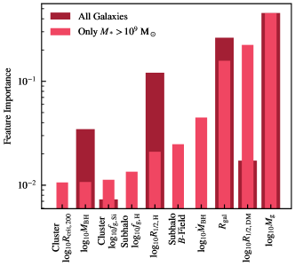
In Fig. 15, we show the results of our machine learning pipeline from Section 4, applied to galaxies with a stellar mass $M_{*}>10^{9}$ M_⊙ only, to test how our results change when considering what would be typically considered ‘well resolved’ galaxies only. The important features are nearly identical to those when we train the pipeline on all substructures as in Fig. 6, with the only major missing important feature the stellar half-mass sizes. This is expected, as demonstrated in Fig. 10, the differences in stellar profiles were mainly powered by the lowest-mass galaxies and were only marginally resolved in the TNG-300 simulation.

The black hole mass feature is replaced with the black hole accretion rate, but again this is simply used for occupation checking. The final, somewhat important, feature that is new here is the Subhalo $B-$field. This feature is somewhat degenerate with the gas mass, with backsplash haloes that retain gas having relatively low magnetic field strengths due to their low gas fraction.

As the same qualitative trends remain from our main results, and there are potentially interesting features shown in the $10^{8}<M_{*}/{\rm M}_{\odot}<10^{9}$ mass range, in the main text we retain the larger sample.

References

- Anglés-Alcázar et al. (2017) Anglés-Alcázar D., Davé R., Faucher-Giguère C.-A., Özel F., Hopkins P. F., 2017, MNRAS, 464, 2840
- Bahé et al. (2013) Bahé Y. M., McCarthy I. G., Balogh M. L., Font A. S., 2013, MNRAS, 430, 3017
- Bahé et al. (2021) Bahé Y. M., et al., 2021, arXiv e-prints, p. arXiv:2109.01489
- Bakels et al. (2021) Bakels L., Ludlow A. D., Power C., 2021, MNRAS, 501, 5948
- Balogh et al. (2000) Balogh M. L., Navarro J. F., Morris S. L., 2000, ApJ, 540, 113
- Barnes et al. (2017) Barnes D. J., et al., 2017, MNRAS, 471, 1088
- Barnes et al. (2018) Barnes D. J., et al., 2018, MNRAS, 481, 1809
- Bassini et al. (2019) Bassini L., et al., 2019, A&A, 630, A144
- Bassini et al. (2020) Bassini L., et al., 2020, A&A, 642, A37
- Benavides et al. (2021) Benavides J. A., et al., 2021, Nature Astronomy, 5, 1255
- Borrow & Borrisov (2020) Borrow J., Borrisov A., 2020, The Journal of Open Source Software, 5, 2430
- Borrow & Kelly (2021) Borrow J., Kelly A. J., 2021, arXiv e-prints, p. arXiv:2106.05281
- Campbell et al. (2017) Campbell D. J. R., et al., 2017, MNRAS, 469, 2335
- Carleton et al. (2019) Carleton T., Errani R., Cooper M., Kaplinghat M., Peñarrubia J., Guo Y., 2019, MNRAS, 485, 382
- Crain et al. (2015) Crain R. A., et al., 2015, MNRAS, 450, 1937
- Dolag et al. (2009) Dolag K., Borgani S., Murante G., Springel V., 2009, MNRAS, 399, 497
- Donnari et al. (2019) Donnari M., et al., 2019, MNRAS, 485, 4817
- Dubois et al. (2012) Dubois Y., Devriendt J., Slyz A., Teyssier R., 2012, MNRAS, 420, 2662
- Duffy et al. (2010) Duffy A. R., Schaye J., Kay S. T., Dalla Vecchia C., Battye R. A., Booth C. M., 2010, MNRAS, 405, 2161
- Farid et al. (2022) Farid D., Aung H., Nagai D., Farahi A., Rozo E., 2022, arXiv e-prints, p. arXiv:2205.01700
- Genel et al. (2018) Genel S., et al., 2018, MNRAS, 474, 3976
- Genel et al. (2019) Genel S., et al., 2019, ApJ, 871, 21
- Gill et al. (2005) Gill S. P. D., Knebe A., Gibson B. K., 2005, MNRAS, 356, 1327
- Haggar et al. (2020) Haggar R., Gray M. E., Pearce F. R., Knebe A., Cui W., Mostoghiu R., Yepes G., 2020, MNRAS, 492, 6074
- Haidar et al. (2022) Haidar H., et al., 2022, arXiv e-prints, p. arXiv:2201.09888
- Hansen et al. (2009) Hansen S. M., Sheldon E. S., Wechsler R. H., Koester B. P., 2009, ApJ, 699, 1333
- Harris et al. (2020) Harris C. R., et al., 2020, Nature, 585, 357
- Hunter (2007) Hunter J. D., 2007, Computing in Science and Engineering, 9, 90
- Jiang & van den Bosch (2016) Jiang F., van den Bosch F. C., 2016, MNRAS, 458, 2848
- Jones et al. (2021) Jones M. G., Bennet P., Mutlu-Pakdil B., Sand D. J., Spekkens K., Crnojević D., Karunakaran A., Zaritsky D., 2021, ApJ, 919, 72
- Keller et al. (2019) Keller B. W., Wadsley J. W., Wang L., Kruijssen J. M. D., 2019, MNRAS, 482, 2244
- Kilborn et al. (2005) Kilborn V. A., Koribalski B. S., Forbes D. A., Barnes D. G., Musgrave R. C., 2005, MNRAS, 356, 77
- Knebe et al. (2011) Knebe A., Libeskind N. I., Knollmann S. R., Martinez-Vaquero L. A., Yepes G., Gottlöber S., Hoffman Y., 2011, MNRAS, 412, 529
- Knebe et al. (2020) Knebe A., et al., 2020, MNRAS, 495, 3002
- Koda et al. (2015) Koda J., Yagi M., Yamanoi H., Komiyama Y., 2015, ApJ, 807, L2
- Ludlow et al. (2009) Ludlow A. D., Navarro J. F., Springel V., Jenkins A., Frenk C. S., Helmi A., 2009, ApJ, 692, 931
- Ludlow et al. (2019a) Ludlow A. D., Schaye J., Schaller M., Richings J., 2019a, MNRAS, 488, L123
- Ludlow et al. (2019b) Ludlow A. D., Schaye J., Bower R., 2019b, MNRAS, 488, 3663
- Ludlow et al. (2020) Ludlow A. D., Schaye J., Schaller M., Bower R., 2020, MNRAS, 493, 2926
- Ludlow et al. (2021) Ludlow A. D., Fall S. M., Schaye J., Obreschkow D., 2021, MNRAS, 508, 5114
- Mamon et al. (2004) Mamon G. A., Sanchis T., Salvador-Solé E., Solanes J. M., 2004, A&A, 414, 445
- Marinacci et al. (2018) Marinacci F., et al., 2018, MNRAS, 480, 5113
- McCarthy et al. (2017) McCarthy I. G., Schaye J., Bird S., Le Brun A. M. C., 2017, MNRAS, 465, 2936
- Naiman et al. (2018) Naiman J. P., et al., 2018, MNRAS, 477, 1206
- Nelson et al. (2018) Nelson D., et al., 2018, MNRAS, 475, 624
- Nelson et al. (2019) Nelson D., et al., 2019, Computational Astrophysics and Cosmology, 6, 2
- O’Neil et al. (2021) O’Neil S., Barnes D. J., Vogelsberger M., Diemer B., 2021, MNRAS, 504, 4649
- O’Neil et al. (2022) O’Neil S., Borrow J., Vogelsberger M., Diemer B., 2022, MNRAS, 513, 835
- Pedregosa et al. (2011) Pedregosa F., et al., 2011, Journal of Machine Learning Research, 12, 2825
- Pillepich et al. (2018a) Pillepich A., et al., 2018a, MNRAS, 473, 4077
- Pillepich et al. (2018b) Pillepich A., et al., 2018b, MNRAS, 475, 648
- Pillepich et al. (2019) Pillepich A., et al., 2019, MNRAS, 490, 3196
- Planck Collaboration et al. (2016) Planck Collaboration et al., 2016, A&A, 594, A13
- Ragone-Figueroa et al. (2013) Ragone-Figueroa C., Granato G. L., Murante G., Borgani S., Cui W., 2013, MNRAS, 436, 1750
- Ragone-Figueroa et al. (2018) Ragone-Figueroa C., Granato G. L., Ferraro M. E., Murante G., Biffi V., Borgani S., Planelles S., Rasia E., 2018, MNRAS, 479, 1125
- Sanchis et al. (2004) Sanchis T., Mamon G. A., Salvador-Solé E., Solanes J. M., 2004, A&A, 418, 393
- Schaye et al. (2015) Schaye J., et al., 2015, MNRAS, 446, 521
- Simpson et al. (2018) Simpson C. M., Grand R. J. J., Gómez F. A., Marinacci F., Pakmor R., Springel V., Campbell D. J. R., Frenk C. S., 2018, MNRAS, 478, 548
- Somerville & Davé (2015) Somerville R. S., Davé R., 2015, ARA&A, 53, 51
- Springel (2011) Springel V., 2011, in Computational Star Formation. pp 203–206, doi:10.1017/S1743921311000378
- Springel & Hernquist (2003) Springel V., Hernquist L., 2003, MNRAS, 339, 289
- Springel et al. (2005) Springel V., et al., 2005, Nature, 435, 629
- Springel et al. (2018) Springel V., et al., 2018, MNRAS, 475, 676
- Tonnesen & Bryan (2009) Tonnesen S., Bryan G. L., 2009, ApJ, 694, 789
- Tremmel et al. (2017) Tremmel M., Karcher M., Governato F., Volonteri M., Quinn T. R., Pontzen A., Anderson L., Bellovary J., 2017, MNRAS, 470, 1121
- Tremmel et al. (2020) Tremmel M., Wright A. C., Brooks A. M., Munshi F., Nagai D., Quinn T. R., 2020, MNRAS, 497, 2786
- Trujillo (2021) Trujillo I., 2021, Nature Astronomy, 5, 1182
- Van Rossum & Drake Jr (1995) Van Rossum G., Drake Jr F. L., 1995, Python reference manual. Centrum voor Wiskunde en Informatica Amsterdam
- Virtanen et al. (2020) Virtanen P., et al., 2020, Nature Methods, 17, 261
- Vogelsberger et al. (2013) Vogelsberger M., Genel S., Sijacki D., Torrey P., Springel V., Hernquist L., 2013, MNRAS, 436, 3031
- Vogelsberger et al. (2014a) Vogelsberger M., et al., 2014a, MNRAS, 444, 1518
- Vogelsberger et al. (2014b) Vogelsberger M., et al., 2014b, Nature, 509, 177
- Vogelsberger et al. (2018) Vogelsberger M., et al., 2018, MNRAS, 474, 2073
- Vogelsberger et al. (2020) Vogelsberger M., Marinacci F., Torrey P., Puchwein E., 2020, Nature Reviews Physics, 2, 42
- Weinberger et al. (2017) Weinberger R., et al., 2017, MNRAS, 465, 3291
- Weinberger et al. (2018) Weinberger R., et al., 2018, MNRAS, 479, 4056
- Weinberger et al. (2020) Weinberger R., Springel V., Pakmor R., 2020, ApJS, 248, 32
- Wiersma et al. (2009) Wiersma R. P. C., Schaye J., Smith B. D., 2009, MNRAS, 393, 99
- de los Rios et al. (2021) de los Rios M., Martínez H. J., Coenda V., Muriel H., Ruiz A. N., Vega-Martínez C. A., Cora S. A., 2021, MNRAS, 500, 1784
- van Dokkum et al. (2015) van Dokkum P. G., Abraham R., Merritt A., Zhang J., Geha M., Conroy C., 2015, ApJ, 798, L45
- van den Bosch (2017) van den Bosch F. C., 2017, MNRAS, 468, 885
- van den Bosch & Ogiya (2018) van den Bosch F. C., Ogiya G., 2018, MNRAS, 475, 4066
- van den Bosch et al. (2018) van den Bosch F. C., Ogiya G., Hahn O., Burkert A., 2018, MNRAS, 474, 3043