Diversity vs. Recognizability: Human-like generalization in one-shot generative models

Abstract

Robust generalization to new concepts has long remained a distinctive feature of human intelligence. However, recent progress in deep generative models has now led to neural architectures capable of synthesizing novel instances of unknown visual concepts from a single training example. Yet, a more precise comparison between these models and humans is not possible because existing performance metrics for generative models (i.e., FID, IS, likelihood) are not appropriate for the one-shot generation scenario. Here, we propose a new framework to evaluate one-shot generative models along two axes: sample recognizability vs. diversity (i.e., intra-class variability). Using this framework, we perform a systematic evaluation of representative one-shot generative models on the Omniglot handwritten dataset. We first show that GAN-like and VAE-like models fall on opposite ends of the diversity-recognizability space. Extensive analyses of the effect of key model parameters further revealed that spatial attention and context integration have a linear contribution to the diversity-recognizability trade-off. In contrast, disentanglement transports the model along a parabolic curve that could be used to maximize recognizability. Using the diversity-recognizability framework, we were able to identify models and parameters that closely approximate human data.

1 Introduction

Our ability to learn and generalize from a limited number of samples is a hallmark of human cognition. In language, scientists have long highlighted how little training data children need in comparison to the richness and complexity of the language they learn so efficiently to master [12, 40]. Similarly, children and adults alike are able to learn novel object categories from as little as a single training example [17, 8]. From a computational point of view, such feats are remarkable because they suggest that learners must be relying on inductive biases to overcome such challenges [33] – from an ability to detect suspicious coincidences or ’non-accidental’ features [43, 52] to exploiting the principle of compositionality [32, 33].

While a common criticism of modern AI approaches is their reliance on large training datasets, progress in one-shot categorization has been significant. One-shot categorization involves predicting an image category based on a unique training sample per class. Multiple algorithms have been proposed including meta-learning algorithms [18, 46, 14, 37] or metric-learning algorithms [47, 31, 48] that are now starting to approach human accuracy. Perhaps a less studied problem is the one-shot generation problem – aimed at creating new variations of a prototypical shape seen only once. Since the seminal work of  Lake et al. [32] who introduced the Bayesian Program Learning algorithm, only a handful of promising one-shot generative algorithms have been proposed [42, 15, 1] (see section 2.2 for a more exhaustive description of prior work).

Why have so few algorithms for one-shot image generation vs. image categorization been proposed? We argue that one of the main reasons for this lack of progress is the absence of an adequate evaluation metric. As of today, one-shot generative models are evaluated using methods initially developed for models producing samples that belong to the training categories and trained on large datasets. Those metrics include the likelihood, the FID (Frechet Inception Distance), or the IS (Inception Score). In the one-shot image generation scenario in which training images are scarce and the generated samples represent new visual concepts, the likelihood, the FID, and the IS are biased [3, 13, 38] (see 2.1 for more details). These limitations urge us to look for new metrics tailored for one-shot image generation.

Figure 1: The diversity vs. recognizability framework. The best possible samples for good generalization (green area) are those that match the intra-class variations (i.e., remain within decision boundaries; Box $1$). Bad samples associated with poor generalization (red area) include strategies that involve exact copies of the prototype (Box $2$) and samples that exceed the intra-class variability (Box $3$).

Recent psychophysics work [52] has characterized humans’ ability for one-shot generation along two main axes: samples diversity (i.e., intra-class variability) and samples recognizability (i.e., how easy or hard they are to classify). According to this framework, ideal generalization corresponds to a combination of high recognizability and high diversity. As illustrated in Fig. 1, an ideal model should be able to generate samples that span the entire space within the decision boundary of a classifier (Box $1$). In comparison, the model of Box $2$ has learned to make identical copies of the prototype (i.e., low diversity but high accuracy). Such a model has failed to generalize the visual concept exemplified by the prototype. Similarly, if the model’s samples are so diverse that they cannot be recognized accurately as shown in the Box $3$ of Fig. 1, then the generated samples won’t look like the prototype.

Here, we borrow from this work and adapt it to create the first framework to evaluate and compare humans and one-shot generative models. Using this framework, we systematically evaluate an array of representative one-shot generative models on the Omniglot dataset [32]. We show that GAN-like and VAE-like one-shot generative models fall on opposite ends of the diversity-recognizability space: GAN-like models fall on the high recognizability — low diversity end of the space while VAE-like models fall on the low recognizability — high diversity end of the space. We further study some key model parameters that modulate spatial attention, context integration, and disentanglement. Our results suggest that spatial attention and context have an (almost) linear effect on the diversity vs. recognizability trade-off. In contrast, varying the disentanglement moves the models on a parabolic curve that could be used to maximize the recognizability. Last but not least, we have leveraged the diversity vs. recognizability space to identify models and parameters that best approximate the human data on the Omniglot handwritten dataset.

2 Related work

2.1 Metrics to evaluate generative models and their limitations for one-shot generation tasks

Different types of generative models are typically evaluated using different metrics. On the one hand, likelihood-based algorithms (e.g., VAE [29], PixelCNN [39], GLOW [30], etc.) are evaluated using their own objective function applied on a testing set. Likelihood provides a direct estimate of the KL divergence between the data points and the model’s samples. On the other hand, implicit generative models such as Generative Adversarial Networks (GANs) [20] for which the loss function cannot be used, are typically evaluated using other scores such as the Inception Score (IS) [45] or Frechet Inception Distance (FID) [22]. IS and FID are heuristic measures used to aggregate both the sample quality and diversity in one single score. The IS scores a sample quality according to the confidence with which an Inception v3 Net [49] assigns the correct class label to it. The FID score is the Wasserstein-2 distance between two Gaussian distributions: one fitted on the features of the data distribution and the other on the features of the model distribution (the features are also extracted from an Inception v3 Network).

All these metrics are problematic for the one-shot generation scenario for $2$ main reasons that are intrinsically related to the task: the low number of samples per class, and the dissimilarity between training and testing visual concepts. IS and FID rely on statistical distances (either KL divergence for IS or Wasserstein-2 distance for FID) that require a high number of data points $N$ to produce an unbiased estimator of the distance. Even when used in the traditional settings (i.e., $N=50000$), it has been demonstrated that both scores are biased [13]. This is to be compared with the $N=20$ samples typically available in popular few-shot learning datasets such as Omniglot [32]. Another problem caused by the limited number of samples per class in the training set is the overfitting of the Inception Net used to extract the features to compute the IS and FID [7]. To illustrate this phenomenon we have conducted a small control experiment in which we have trained a standard classifier to recognize images from the Omniglot datasets (see S17). In this experiment, we have used 18 samples per classes for training and 2 samples per classes for testing. In Fig. S21a, we observe an increase of the testing loss while the training loss is decreasing. This is a clear sign of overfitting. Note that this overfitting is not happening when the standard classifier is replaced by a one-shot (or few-shot) classifier. This control experiment show that standard classifier are not adapted to extract relevant features in the low-data regime. Consequently, IS and FID are not suitable in the low-data regime.

The second limitation of these metrics appears because the training and the testing samples are too dissimilar. Likelihood scores are known to yield higher scores for out-of-domain data compared to in-domain data [38]. Therefore, the evaluation of the novel visual concepts generated by one-shot generative models will be biased toward higher scores. In addition, both FID and IS rely on distance between features extracted by an Inception Net which comes with no guarantee that it will produce meaningful features for novel categories. For example, class misalignment has been reported when the Inception Net was trained on ImageNet and tested on CIFAR10 [3]. Because of all the aforementioned limitations, it is pretty clear that new procedures are needed to evaluate the performance of few-shot generative algorithms.

2.2 One-shot generative models

One can distinguish between two broad classes of one-shot generative models: structured models and statistical models [16]. Structured models have strong inductive biases and rigid parametric assumptions based on a priori knowledge such as for example a given hierarchy of features, a known grammar or program [44]. A prominent example of a structured model includes the very first algorithm for one-shot image generation, the Bayesian Program Learning (BPL) model [32]. Statistical models learn visual concepts by learning statistical regularities between observed patterns [42, 15, 19]. Here, we focus on representative architectures of one-shot generative statistical models, which we summarize below.

• VAE with Spatial Transformer Network (VAE-STN) [42]. The VAE-STN is a sequential and conditional Variational Auto-Encoder (VAE) constructing images iteratively. The VAE-STN algorithm uses a recurrent neural network (i.e., an LSTM) to encode the sequence of local patches extracted by an attentional module. A key ingredient of the VAE-STN is an attention module composed of a Spatial Transformer Network (STN) [26] to learn to shift attention to different locations of the input image. The STN is a trainable module to learn all possible affine transformations (i.e., translation, scaling, rotation, shearing) of an input image (see S8 for samples and details of the VAE-STN).

• Neural statistician (VAE-NS) [15]: The Neural Statistician is an extension of the conditional VAE model including contextual information. Therefore, in addition to learning an approximate inference network over latent variables for every image in the set (as done in a VAE), the approximate inference is also implemented over another latent variable, called the context variable, that is specific to the considered visual concept. The context inference network is fed with a small set of images representing variations of a given visual concept. The VAE-NS has been extended to include attention and hierarchical factorization of the generative process [19] (see S9 for samples and details of the VAE-NS).

• Data-Augmentation GAN (DA-GAN) [1]: Data-Augmentation GAN is a generative adversarial network conditioned on a prototype image. The DA-GAN generator is fed with a concatenation of a vector drawn from a normal distribution and a compressed representation of the prototype. The discriminator is trained to differentiate images produced by the generator from images of the dataset, while the generator has to fool the discriminator. We have trained $2$ different DA-GAN, one is based on the U-Net architecture (DA-GAN-UN) and the other one on the ResNet architecture (DA-GAN-RN) (see S10 for samples and details of the DA-GAN-UN and  S11 for samples and details of the DA-GAN-RN).

All these models are generative models conditioned by an image prototype extracted from the training or the test set. The way we have selected the prototypes is detailed in Eq. 1. To the best of our knowledge, these models offer a representative set of one-shot generative models. We have reproduced all these models (sometimes with our own implementation when it was not available online). Our code could be found at https://github.com/serre-lab/diversity_vs_recognizability.

3 The diversity vs. accuracy framework

Let $\{x_{i}^{j}\}$ be a dataset composed of K concepts (i.e., classes) with N samples each ($i\in[\![1,N]\!]$ and $j\in[\![1,K]\!]$). The framework we propose aims at evaluating the performance of a generative model $p_{\theta}$, parameterized by $\theta$, that produces new images $v_{i}^{j}$ based on a single sample (or prototype) of a concept given to the generator $\tilde{x}^{j}$ (i.e., $v_{i}^{j}\sim p_{\theta}(\cdot|\tilde{x}^{j})$). For each concept $j$, we define a prototype as the sample closest to the center of mass for the concept $j$:

$$\tilde{x}^{j}=x_{i^{*}}^{j}\quad\text{s.t.}\quad i^{*}=\operatorname*{argmin}_{i}\left\lVert f(x_{i}^{j})-\frac{1}{N}\sum_{i=1}^{N}f(x_{i}^{j})\right\rVert_{2}$$ (1)

In Eq. 1, $f$ denotes a function that projects the input image from the pixel space to a feature space. We will detail the feature extractor $f$ shortly. Note that this definition of a prototype is not unique (one could also select the prototype randomly within individual classes $j$), nevertheless this selection mechanism is a guarantee that the selected sample will be representative of the concept.

Dataset. In this article, we use the Omniglot dataset [32] with a weak generalization split [42]. Omniglot is composed of binary images representing $1,623$ classes of handwritten letters and symbols (extracted from $50$ different alphabets) with just $20$ samples per class. We have downsampled the original dataset to be $50\times 50$ pixels. The weak generalization split consists of a training set composed of all available symbols minus $3$ symbols per alphabet which are left aside for the test set. It is said to be weak because all the alphabets were shown during the training process (albeit not all symbols in those alphabets). As the Omniglot dataset is hand-written by humans, we consider that these samples reflect a human generative process and we refer to this later as the human model.

Diversity. In the proposed framework, diversity refers to the intra-class variability of the samples produced by a generative model $p_{\theta}(\cdot|\tilde{x}^{j})$. For a given prototype $\tilde{x}^{j}$, we compute the diversity as the standard deviation of the generated samples in the feature space $f$:

$$\sigma_{p_{\theta}}^{j}=\sqrt{\frac{1}{N-1}\sum_{i=1}^{N}\Big{(}f(v_{i}^{j})-\frac{1}{N}\sum_{i=1}^{N}f(v_{i}^{j})\Big{)}^{2}}\quad\text{s.t.}\quad v_{i}^{j}\sim p_{\theta}(\cdot|\tilde{x}^{j})$$ (2)

We use the Bessel-corrected standard deviation to keep a good estimate of the data dispersion despite the relatively small number of samples (e.g., $N=20$ for the Omniglot dataset used here). To verify that this diversity measure is robust to the specific choice of the feature extractor $f$, we explored two different settings: features learned with class supervision by a Prototypical Net [47] and features learned with self-supervision by a SimCLR network [10]. In both cases, we extracted the features from the first fully-connected layer following the last convolutional layer. The Prototypical Net was optimized so that images that belong to the same category share similar latent representations as measured by the $\ell_{2}$-norm. Similarly, SimCLR leverages a contrastive loss to define a latent representation such that a sample is more similar to its augmented version than to other image samples. In SimCLR, this similarity is computed with cosine similarity. These two approaches represent two ends of a continuum of methods to learn suitable representational spaces without the need to explicitly learn to classify images and are thus more suitable for few-shot learning tasks [35]. For the sake of comparison, we have used the exact same network architecture for both feature extractors (see sections S1 and S2 for more details on Prototypical Net and SimCLR, respectively).

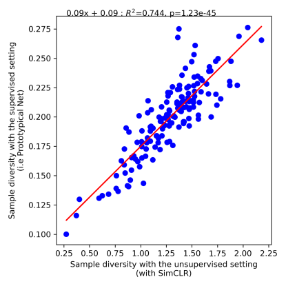
We computed the samples diversity for all $150$ categories of the Omniglot test set (i.e., $v_{i}^{j}=x_{i}^{j}$ in this experiment) using both the supervised and unsupervised settings. We found a high linear correlation ($\rho=0.86$, p-value $<10^{-5}$) and a high rank-order Spearman correlation ($\rho=0.85$, p-value $<10^{-5}$) between the two settings (see section S3.1). Hence, the two feature extraction methods produce comparable diversity measures and henceforth, we will report results using the unsupervised setting.

As an additional control, we have also verified that the SimCLR metric is robust to changes to the augmentation method used (see section S3.3) and to the specific choice of the dispersion metric (see section S3.2 for more details on this comparison). We have compared the feature space of the Prototypical Net and SimCLR using a t-SNE analysis (see section S3.4). We observed a strong clustering of samples belonging to the same category for both networks. It suggests that the augmentation methods used by the SimCLR contrastive loss are sufficient to disentangle the class information.

Fig. 2 shows the $10$ concepts from the Omniglot test set with the lowest and highest samples diversity, respectively (for more diversity-ranked concepts with unsupervised or supervised setting, see sections S4 and  S5, respectively). One can see that the proposed diversity metric is qualitatively similar to human judgment. Concepts with low diversity are composed of very few relatively basic strokes (e.g., lines, dots, etc) with little room for any kind of “creativity” in the generation process while more diverse concepts are composed of more numerous and more complex stroke combinations with many more opportunities for creativity.

Figure 2: Samples from the top 10 Omniglot concepts (test set) associated with the lowest (a) vs. highest diversity (b). The different concepts are ranked vertically from less diverse to more diverse. Prototypes for individual concepts are shown within a red box next to actual class samples.

Recognizability. We evaluate the recognizability of the samples produced by the one-shot generative models by leveraging one-shot classification models. As demonstrated in S17, it is also possible to use a few-shot classifier to evaluate the recognizability. We prefer one-shot classifier to match the settings proposed in [32]. In order to make sure our classification accuracy measure is robust to the choice of the model, we test different models which belong to the two main approaches used in machine learning for one-shot classification: metric learning and meta-learning [35]. We selected the Prototypical Net [47] as a representative metric-learning approach and the Model-Agnostic Meta-Learning (MAML) [18] model as a representative meta-learning approach. Both models were trained and tested in a 1-shot 20-ways setting (see section S6 for more details on the MAML architecture and training details). We report a high Pearson (negative) correlation between the logits produced by Prototypical Net and MAML ($\rho=-0.60$, p-value $<10^{-5}$) as well as a strong Spearman rank-order correlation between the classification accuracy of both networks ($\rho=0.62$, p-value $<10^{-5}$). See section S7 for more details about this control experiment. Hence, our recognizability metric is robust to the choice of the one-shot classification model (even when those models are leveraging different approaches) and henceforth, we will report results using the Prototypical Net model.

4 Results

4.1 GAN-like vs. VAE-like models

For all algorithms listed in section 2.2 we have explored different hyper-parameters (see section 4.2 for more details), leading to various models represented in the diversity vs. recognizability plot in Fig. 3a. In this figure, we have reduced each model to a single point by averaging the diversity and recognizability over all classes of the Omniglot testing set. The black star corresponds to the human model, and colored data points are computed based on the samples generated by the VAE-NS, VAE-STN, DA-GAN-UN and the DA-GAN-RN. The base architectures for all algorithms (highlighted with bigger points in Fig. 3a) have a comparable number of parameters ($\approx$6-7 M, see S8, S9 and S10 for more details on the base architectures).

We observe that the GAN-like models (i.e., DA-GAN-UN and DA-GAN-RN) tend to be located at the upper left side of the graph while VAE-like models (i.e., VAE-NS and VAE-STN) spread on the right side of the graph. Therefore, the GAN-like models produce very recognizable samples that are highly similar to each other (high recognizability and low diversity). In contrast, VAE-like models generate more diverse but less recognizable samples. The samples in Fig. 3b illustrate this observation. The difference between GAN and VAE-like samples could be explained by their loss functions [36]. The GANs’ adversarial loss tends to drop some of the modes of the training distribution. In general, the distribution learned by GANs put excessive mass on the more likely modes but discards secondary modes [2]. This phenomenon leads to sharp and recognizable generations at the cost of reduced samples diversity. On the other hand, VAEs (and likelihood-based models in general) are suffering from over-generalization: they cover all the modes of the training distribution and put mass in spurious regions [4]. We refer the reader to Fig. 4 of Lucas et al. [36] for an illustration of mode dropping in GANs and over-generalization in VAEs. Our diversity vs. recognizability plot in Fig. 3a shows that this phenomenon is holding even when the testing distribution is different from the training distribution as in the case of the one-shot generation scenario.

Figure 3: (a) Diversity vs. recognizability plot for all tested models (colored data points) and human (black star). Each data point corresponds to the mean diversity and recognizability over all classes of the Omniglot test set. Bigger circles correspond to the base architecture of each model that all have a comparable number of parameters ($\approx 6-7$M). The human data-point is computed based on the testing samples of the Omniglot dataset. (b) Samples produced by the different models in their base architectures (corresponding to the bigger circles in Fig. 3a). Prototypes for individual concepts are shown within a red box next to actual class samples.

4.2 VAE-NS vs. VAE-STN

In this section we compare some key hyper-parameters of the VAE-NS and VAE-STN. The core idea of the VAE-NS is to integrate context information to the sample generation process. During training, the context is composed of several samples that all represent variations of the same visual concept. Those samples are passed in a separate encoder to extract a context statistics (denoted $c$ in  S9) used to condition the generative process. During the testing phase, the VAE-NS infers the context statistics using a single image (i.e., the prototype). We evaluate the effect of the context on the position of the VAE-NS models on the diversity-recognizability space by varying the number of samples used to compute the context statistics during the training phase (from $2$ to $20$ samples). Importantly, varying the number of context samples do not change the number of parameters of the network. For all tested runs, we observe a monotonic decrease of the samples diversity (see Fig. S13a) and a monotonic increase of the samples recognizability (see Fig. S13b) when the number of context samples is increased. In the diversity-recognizability space, the resulting curve is monotonically transporting models from the lower-right side to the upper-left side of the plot (see Fig. 4a, dark blue curve). The effect of the number of context samples is large: the diversity is almost divided by $2$ (from $2.4$ to $1.2$) and the classification accuracy is increased by $80\%$ (from $53\%$ to $96\%$). This result suggests that increasing the number of context samples for a given visual concept helps the generative model to identify the properties and the features that are crucial for good recognition, but hurts the diversity of the generated samples.

Figure 4: (a) Effect of the number of context samples of the VAE-NS and attentional steps of the VAE-STN. Each data point represents a model with a different number of context samples for the VAE-NS (ranging from $2$ to $20$) or a different number of attentional steps for the VAE-STN (ranging from $20$ to $90$). The base architectures, highlighted with a bigger circle, correspond to $10$ context samples and $60$ attentional steps for the VAE-NS and VAE-STN respectively. (b) Effect of $\beta$. The base architectures correspond to a $\beta=1$. In all curves, solid lines represent the mean of the parametric curves over $3$ different runs. Shaded areas are computing using the standard deviation over $3$ different runs. Arrows show the direction in which the tested variables (context samples, attention steps or $\beta$) are increased.

In contrast to the VAE-NS, the VAE-STN uses spatial attention to sequentially attend to sub-parts of the image to decompose it into simpler elements. These sub-parts are then easier to encode and synthesize. In the VAE-STN, one can vary the number of attentional steps (i.e., the number of attended locations) to modulate spatial attention. Importantly, varying the number of attentional steps does not change the number of parameters. We have varied the number of attentional steps from $20$ to $90$. The relationship between the number of attentional steps, the samples diversity, and the samples recognizability is non-monotonic. We have used a parametric curve fitting method (i.e., the least curve fitting method from [21]) to parameterize the curve while maintaining the order of the data point (see  S13 for more details on the fitting procedure). We report a convex parabolic relationship between the number of attentional steps and the samples diversity (see Fig. S14a). This curve is minimal at $60$ steps. We observe a concave parabolic relationship between the number of attentional steps and the recognizability of samples. This curve is maximal at $60$ attentional steps (see Fig. S14b). In Fig. 4b we have plotted the parametric fit illustrating the position of the VAE-STN models in the diversity-recognizability space when one increases the number of attentional steps (the light blue curve). This curve follows a quasi-linear trend with a sharp turn-around (at $60$ attentional steps). The effect of the number of attentional steps on the diversity-recognizability is limited compared to the effect of the number of context samples.

Both VAE-NS and VAE-STN are trained to maximize the Evidence Lower Bound (ELBO), it is then possible to tune the weight of the prior in the loss function. One can operate such a modulation by changing the $\beta$ coefficient in the ELBO loss function [24]. We refer the reader to S15 for more mathematical details about the ELBO. A high $\beta$ value enforces the latent variable to be closer to a normal distribution and increases the information bottleneck in the latent space. Increasing $\beta$ is known to force the disentanglement of the generative factors [9]. We observe a monotonic decreasing relationship between the value of $\beta$ and the samples diversity for both the VAE-STN and the VAE-NS (see Fig. S15a and Fig. S16a, respectively). We report a concave parabolic relationship between $\beta$ and the samples recognizability. We use the least curve fitting method to find the optimal parabolic curves [21]. This curve is maximal at $\beta=2.5$ for the VAE-STN and at $\beta=3$ for the VAE-NS (see Fig. S15b and Fig. S16b, respectively). The overall effect of $\beta$ on the position of the VAE-like models on the diversity-recognizability space is relatively similar for both the VAE-STN and the VAE-NS and follows a clear parabolic trend. These curves demonstrate that one could modulate the value of $\beta$ to maximize the recognizability. In general, we observe that the variable controlling the context-size in the VAE-NS is the one having the biggest impact on the diversity-recognizability space.

We have also varied the architecture of the DA-GAN-UN, DA-GAN-RN, VAE-NS, and VAE-STN by changing the size of the latent space. We did not find any common trend between the size of the latent variable, the diversity, and the recognizability (see S16 for more details). We observe that the DA-GAN-UN tends to produce slightly more recognizable but less diverse samples than the DA-GAN-RN while both architectures have the same number of parameters. It suggests that the extra skip connections included in the U-Net architecture, in between the encoder and the decoder of the DA-GAN-UN, allow to trade diversity for recognizability.

4.3 Comparison with humans

Figure 5: (a) Distribution of average distance to humans for the VAE-NS, VAE-STN, DA-GAN-UN  and DA-GAN-RN. Each data point corresponds to the mean diversity and accuracy over all classes of the Omniglot test set. Squares correspond to the model showing the smallest distance to humans. The distance to humans is calculated with a $\ell_{2}$-norm on the diversity-recognizability space after z-score normalization. The horizontal line denotes the median of the model’s distribution. (b) Distance to humans on $16$ different visual concepts for the VAE-NS and VAE-STN models that best approximate human data (i.e., indicated by a square in Fig. 5a). The visual concepts $1$ to $8$ are selected to minimize the VAE-STN distance to humans, and visual concepts $9$ to $16$ minimize the VAE-NS distance to humans. Images surrounding the radar plot are the prototypes of the visual concepts.

We now compare the tested models with the human data in the diversity-recognizability space. To perform such a comparison, we first normalize all the model’s diversity and recognizability (including humans) using the z-score such that both axes are scaled and centered similarly. Then, for all models, we compute the $\ell_{2}$-distance between models and humans in the diversity-recognizability space. We remind that the human data point is computed using the samples of the Omniglot test set. Distances to humans as well as their distributions are reported for all models in Fig. 5a. The median of VAE-NS models is closer to humans, followed by DA-GAN-UN, DA-GAN-RN and VAE-STN (medians are indicated in Fig. 5a with horizontal bars). The VAE-NS model showing the smallest distance is almost at the human level (see dark blue square Fig. 5a). It has a context size of $20$ samples (the highest possible context size), and a $\beta=2.5$. The VAE-STN model that best approximates human has a $\beta=2.25$ and $60$ attentional steps (see light blue square in Fig. 5a).

So far, we have reduced all models to single points by averaging the diversity and recognizability values over all classes. We now study distances to humans for individual classes and for the VAE-NS and the VAE-STN models showing the shortest distance to humans (indicated by blue squares in Fig. 5a). In Fig. 5b, we report distances to human for these $2$ models and for $16$ visual concepts. The visual concepts $1$ to $8$ and $9$ to $16$ are selected so that they minimize the distance to humans with the VAE-STN and the VAE-NS, respectively. We observe that these visual concepts are different for the VAE-NS and the VAE-STN model. Therefore, both models are well approximating human data for some visual concepts but not for others. Interestingly, we qualitatively observe that the visual concepts $1$ to $8$ look simpler (i.e., made with fewer strokes) than the visual concepts $9$ to $16$. It suggests that the spatial attention mechanism used by VAE-STN provides a better human approximation for simple visual concepts, while the context integration method leveraged by the VAE-NS is more relevant to mimic human data on more complex visual concepts.

5 Discussion

In this article, we have described a novel framework for comparing computational models with human participants on the one-shot generation task. The framework measures the diversity and the recognizability of the produced samples using metrics compatible with the one-shot scenario. To the best of our knowledge, this is the first and only framework specifically tailored to evaluate and compare one-shot image generation models.

Among all tested algorithms, the VAE-NS is the best human approximator on Omniglot (see Fig. 5a). It suggests that the context integration mechanism of the VAE-NS is an important component to reach human-like generalization. Interestingly, motor learning experiments have demonstrated that human generalization performances are also strongly related to contextual information [50]. Interestingly, [51] have demonstrated that a bayesian observer tends to overestimate the intra-class variance when only a few context samples are accessible. Our results are in-line with this finding: Fig. 4a shows an high diversity when the number of context samples is low while the diversity is decreasing when more context samples are available. It suggests that the VAE-NS is acting as a bayesian observer: it overestimates intra-class variance when the context is scarse.

In addition, we demonstrate that one can tune $\beta$ so that the model becomes closer to human data (see Fig. 4b). This is consistent with a prior computational neuroscience study that has shown that disentangled VAEs (with $\beta>1$) provide a good model of face-tuned neurons in the inferotemporal cortex [23]. Our comparison between the VAE-NS and the VAE-STN suggests that a model which uses a spatial attention mechanism better fits human data for simple visual concepts. In contrast, the context integration mechanism of the VAE-NS appears to be a better human approximator for more complex visual concepts. One could thus try to combine both mechanisms towards improving the similarity with human data independent of the complexity of the visual concept. We have also found that GAN-like models (DA-GAN-RN and DA-GAN-UN) better account for human recognizability but do not approximate well the diversity of the human samples. In contrast, VAE-like models (VAE-NS and VAE-STN) better account for human diversity. An interesting approach would be to leverage a hybrid architecture (such as the VAE-GAN [34]) to try to better match human data.

Other candidate ingredients include the ability to harness compositionality [32] or the recurrent processes thought to be crucial for human generalization [54]. Compositionality could be introduced in one-shot generative algorithms by quantizing the latent space (as in the VQVAE [53]). As a result, each coordinate of the latent variable represents an address in a codebook, and the role of the prior is then to combine simpler concepts to generate more complex samples. One promising way to include recurrent processing into generative models is through the predictive coding framework [41]. Predictive Coding suggests that each processing step is part of an inference scheme that minimizes the prediction error [6]. Previous work has demonstrated that such networks are more robust and exhibit improved generalization abilities [5, 11]. All these ingredients could be tested and compared against human abilities using the diversity/recognizability framework we have proposed in this paper.

In the current version of the Omniglot dataset, the intra-class variability does not reflect the human level of creativity. It is mainly due to the experimental protocol in which one asks human participants to copy a given visual concept. The Omniglot dataset could be enriched with more diverse samples, by explicitly asking human participants to be as creative as possible. Other drawing databases with more complex symbols such as Quick Draw! [27] could also be considered to strengthen the comparison with humans.

By decomposing the performance of the one-shot generation task along the recognizability vs. diversity axes we wanted to shed light on the relationship between generalization and creativity (quantified by the samples diversity in our framework). We hope one can make use of our framework to validate key hypotheses about human generalization abilities so that we can better understand the brain. We argue that the best way to reach human-like generalization abilities is to unleash the algorithms’ creativity.

Checklist

1. For all authors…

   1. Do the main claims made in the abstract and introduction accurately reflect the paper’s contributions and scope? [Yes]

   2. Did you describe the limitations of your work? [Yes] Described in the conclusion.

   3. Did you discuss any potential negative societal impacts of your work? [Yes] We have briefly discussed societal impact in S18.

   4. Have you read the ethics review guidelines and ensured that your paper conforms to them? [Yes]

2. If you are including theoretical results…

   1. Did you state the full set of assumptions of all theoretical results? [N/A] No theoretical results

   2. Did you include complete proofs of all theoretical results? [N/A] No theoretical results

3. If you ran experiments…

   1. Did you include the code, data, and instructions needed to reproduce the main experimental results (either in the supplemental material or as a URL)? [Yes] All the codes are available on github ( link given in section 2.2)

   2. Did you specify all the training details (e.g., data splits, hyper-parameters, how they were chosen)? [Yes] All the training details, as well as the architectural details are given in the supplementary materials.

   3. Did you report error bars (e.g., with respect to the random seed after running experiments multiple times)? [Yes] Error bars have been reported on $3$ different runs

   4. Did you include the total amount of compute and the type of resources used (e.g., type of GPUs, internal cluster, or cloud provider)? [Yes] In the Supplementary Information at section  S18

4. If you are using existing assets (e.g., code, data, models) or curating/releasing new assets…

   1. If your work uses existing assets, did you cite the creators? [Yes] All the github links are disclosed in the Supplementary information, and the contributing authors are cited in the main article.

   2. Did you mention the license of the assets? [N/A]

   3. Did you include any new assets either in the supplemental material or as a URL? [Yes] The github link of our code is included in the article

   4. Did you discuss whether and how consent was obtained from people whose data you’re using/curating? [N/A] All assets we are using are publicly available, and do not require any consent

   5. Did you discuss whether the data you are using/curating contains personally identifiable information or offensive content? [N/A] No personal information in Omniglot

5. If you used crowdsourcing or conducted research with human subjects…

   1. Did you include the full text of instructions given to participants and screenshots, if applicable? [N/A]

   2. Did you describe any potential participant risks, with links to Institutional Review Board (IRB) approvals, if applicable? [N/A]

   3. Did you include the estimated hourly wage paid to participants and the total amount spent on participant compensation? [N/A]

Supplementary Information

S1 More details on Prototypical Net

Architecture

Table S1 describes the architecture of the Propotypical Net [47] we are using in this article. We use the Pytorch convention to describe the layers of the network.

Table S1: Description of the Prototypical Net Architecture

Network	Layer	# params
ConvBlock(Inc, Outc)	Conv2d(Inc, Outc, 3, padding=1)	Inc $\times$ Outc $\times$ 3 $\times$ 3 + Outc
	BatchNorm2d(Outc)	2 x Outc
	ReLU	-
	MaxPool2d(2, 2)	-
Prototypical Net	ConvBlock(1, 64)	0.7 K
	ConvBlock(64, 64)	37 K
	ConvBlock(64, 64)	37 K
	ConvBlock(64, 64)	37 K
	Flatten	-
	ReLU	-
	Linear(576, 256)	147 K
	ReLU
	Linear(256, 128)	32 K

The overall number of parameters of the Prototypical Net we are using is around 292 K parameters. The loss of the Prototypical Net is applied on the output of the last fully connected layers (of size $128$). For the computation of the samples diversity, we extract the features on the first fully-connected layer after the last convolutional layer (i.e., of size $256$).

Training details

The Prototypical Net is trained in a 1-shot 60-ways setting and tested on a $1$-shot $20$-ways setting. The size of the query set is always $1$ for both training and testing phase. The model is trained during $80$ epochs, with a batch size of $128$. For training, we are using an Adam optimizer [28] with a learning rate of $1\times 10^{-3}$ (all other parameters of the Adam optimizer are the default ones). We are scheduling the learning rate such that it is divided by $2$ every $20$ epochs.

At the end of the training, the training accuracy (evaluated on 1000 episodes) has reached $100\%$ and the testing accuracy reaches a plateau at $96.55\%$.

S2 More details on SimCLR

S2.1 Architecture and Data Augmentation

The architecture we are using for SimCLR [10] is the exact same than the one used for Prototypical Net (see Table S1). In SimCLR, we also extract the features on the first fully-connected layer after the last convolutional layer (i.e., of size $256$). The augmentations we use are randomly chosen among the $3$ following transformations

• Random resized crop: it crops random portion of the image and resizes it to a given size. $2$ sets of parameters are used for this transformation: the scale and the ratio. The scale parameter specifies the lower and upper bounds for the random area of the crop. The ratio parameter specifies the lower and upper bounds for the random aspect ratio of the crop. Our scale range is ($0.1$, $0.9$) and our ratio range is ($0.8$, $1.2$).

• Random affine transformation: it applies a random affine transformation of the image while keeping the center invariant. The affine transformation is a combination of a rotation (from $-15^{\circ}$ to $15^{\circ}$), a translation (from $-5$ pixels to $5$ pixels), a zoom (with a ratio from $0.75$ to $1.25$) and a shearing (from $-10^{\circ}$ to $10^{\circ}$).

• Random perspective transformation: apply a scale distortion with a certain probability to simulate 3D transformations. The scale distortion we have chosen is $0.5$, and it is applied to the image with a probability of $50\%$

Please see the site https://pytorch.org/vision/main/auto_examples/plot_transforms.html for illustration of the transformations. Note that we have tried different settings for the augmentations (varying the parameters of the augmentations), and we have observed a very limited impact of those settings on the computation of the samples diversity (see S3.3 for more details).

S2.2 Training details

Our SimCLR network is trained for $100$ epochs with a batch size of $128$. We used an RMSprop optimizer [25], with a learning rate of $10^{-3}$ (all other parameters of the RMSprop are the default ones).

S3 Control experiments for the samples diversity computation

S3.1 Comparing the supervised and the unsupervised settings for the computation of the samples diversity

To compare the unsupervised with the supervised setting, we have computed for all of the $150$ classes of the Omniglot testing set the samples diversity. We plot the samples diversity values for each category and for both settings in Fig. S1. We report a linear correlation coefficient $R^{2}=0.74$ and a Spearman rank order correlation $\rho=0.85$ (see Table S2, first line). It does mean that the samples diversity, as computed with one of the setting, is strongly correlated both in terms of rank order and explained variance, with the samples diversity as computed with the other setting.

Figure S1: Comparison of the samples diversity computed by the supervised and the unsupervised settings. Each data point corresponds to a specific class in the Omniglot test set. Here, the samples diversity is computed applying the standard deviation (see Eq. 2) on SimCLR features (for x-axis) or on the features of Prototypical Net (for y-axis)

Table S2: Spearman rank order correlation for different settings

Setting 1	Setting 2	Spearman correlation	p value
Proto. Net + Eq. 2	SimCLR + Eq. 2	$0.85$	$8.99\times 10^{-43}$
Proto. Net + Eq. 3	SimCLR + Eq. 3	$0.71$	$1.47\times 10^{-24}$
Proto. Net + Eq. 2	Proto. Net + Eq. 3	$0.73$	$1.19\times 10^{-26}$
SimCLR + Eq. 2	SimCLR + Eq. 3	$0.63$	$5.21\times 10^{-18}$

S3.2 More control experiments on the effect of the dispersion measure

To make our analysis more robust we have conducted additional control experiments with different measures of dispersion. In Eq. 2 we have presented a classical measure of dispersion that is the standard deviation. Another measure of data dispersion is the pair-wise cosine distance among the samples belonging to the same class:

$$\sigma_{p_{\theta}}^{j}=\sum_{i=1}^{N}\sum_{\begin{subarray}{c}k=1\\ k>i\end{subarray}}^{N}\sqrt{2-2C(f(v_{i}^{j}),f(v_{k}^{j}))}\quad\text{s.t.}\quad v_{i}^{j}\sim p_{\theta}(\cdot|\tilde{x}^{j})\quad\text{and}\quad C(u,v)=\frac{u\cdot v}{\left\lVert u\right\rVert\left\lVert v\right\rVert}$$ (3)

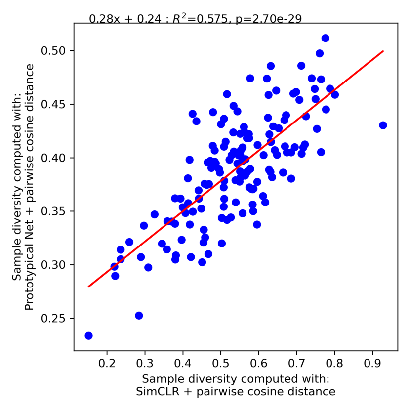
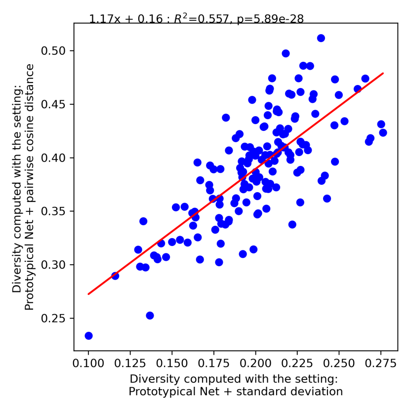
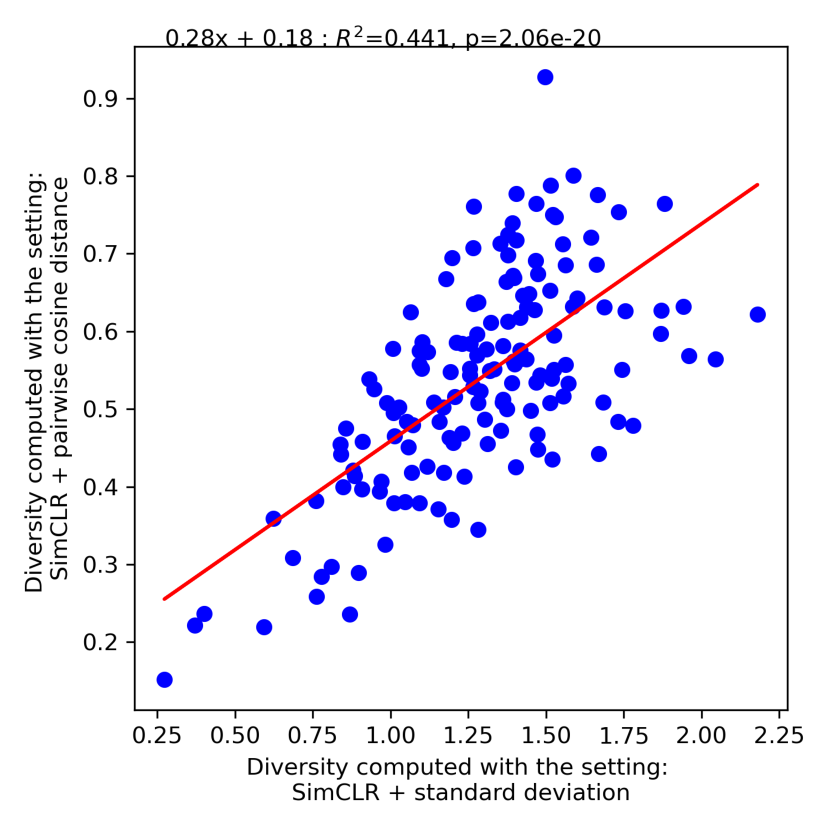
In Eq. 3, $C$ denotes the cosine similarity. In Fig. 2(a), we plot the samples diversity for both feature extraction networks but with a dispersion measure based on the pairwise cosine distance as formulated in Eq. 3. We report a linear correlation of $R^{2}=0.57$ and a Spearman rank order correlation of $\rho=0.71$ (see second line of Table S2). This control experiment suggests that even by using a different dispersion metric (i.e., the pairwise cosine distance), the $2$ feature extraction networks produce samples diversity values that are heavily correlated. This strengthen our observation made in S3.1: the representations produced by the SimCLR and Prototypical Net are similar. Another interesting control experiment is to compare the impact of the dispersion measure on the samples diversity metric. To do so, we have compared the samples diversity computed with one feature extractor (either Prototypical Net in Fig. 2(b) or SimCLR in Fig. 2(c)) but for $2$ different dispersion metrics (i.e., the standard deviation as formulated in Eq. 2 and the pairwise cosine distance as defined in Eq. 3). In both cases, we have a non negligible linear correlation (i.e., $R^{2}>0.44$) and a strong Spearman rank order correlation (i.e., $\rho>0.63$, see third and fourth lines of Table S2). All these control experiments confirm that our computation of the samples diversity is robust to 1) the type of approach we used to extract the features and 2) the measure of dispersion we are using to compute the intraclass variability.

(a) SimCLR + cosine distance vs. Proto Net + cosine distance

(b) Proto Net + standard deviation vs. Proto Net + cosine distance

(c) SimCLR + cosine distance vs. Proto Net + standard deviation

Figure S2: Control experiments when the dispersion metric is the pairwise cosine distance (as defined in Eq. 3). Each point corresponds to a specific class of the Omniglot testing set. In a) we vary the feature extraction network, while keeping the same dispersion metric (i.e., the pairwise cosine distance). In b) and c), we fix the feature extraction network (Prototypical Net for b) and SimCLR for c)) and we vary the dispersion metric (standard deviation for the x-axis or the pairwise cosine distance for the y-axis).

S3.3 Impact of the image augmentation on the diversity measure

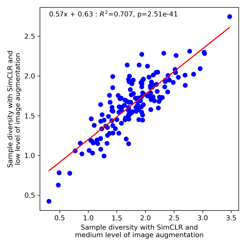
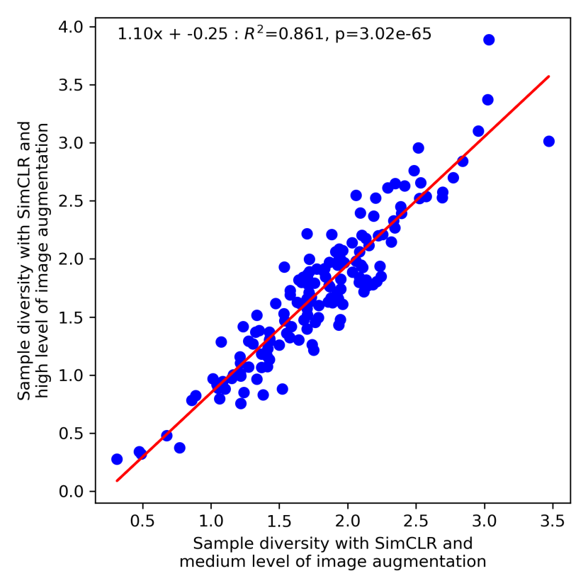
To test the impact of the image augmentations on the SimCLR network we have trained $3$ SimCLR networks with different augmentation levels.

• With moderate level of image augmentation. All the augmentations here are those described in section S2.

• With a low level of image augmentation. Here the scale of the random resized crop is varied from $0.05$ to $0.95$ and the crop ratio is ranging from $0.9$ to $1.1$. The rotation of the affine transformation is ranging from $-7\deg$ to $7\deg$, the translation from $-3$ pixels to $3$ pixels, the zoom from $0.9$ to $1.1$ and the shearing from $-5\deg$ to $5\deg$. The scale distortion applied to the image is $0.25$ (with a probability of $50$%).

• With a high level of image augmentation. In this setting, the scale of the random resized crop is varied from $0.2$ to $0.8$ and the crop ratio is ranging from $0.6$ to $1.4$. The rotation of the affine transformation is ranging from $-30\deg$ to $30\deg$, the translation from $-10$ pixels to $10$ pixels, the zoom from $0.5$ to $1.5$ and the shearing from $-20\deg$ to $20\deg$. The scale distortion applied to the image is $0.75$ (with a probability of $50$%).

In Fig. S3, we compare the samples diversity obtains for each category of the Omniglot testing set when we train the SimCLR network with moderate level of image augmentation and with a low level of image augmentation (see Fig. 3(a)), or with a high level of image augmentation (see Fig. 3(b)). We also report the Spearman correlation in Table S3.

(a) SimCLR with moderate level of image augmentation versus SimCLR with low level of image augmentation

(b) SimCLR with moderate level of image augmentation versus SimCLR with high level of image augmentation

Figure S3: Control experiment to assess the impact of the level of image augmentation on the sample metric as evaluated as a standard deviation in the SimCLR feature space.

Table S3: Spearman rank order correlation for different settings

Setting 1	Setting 2	Spearman correlation	p value
moderate augmentation	light augmentation	$0.79$	$1.7\times 10^{-33}$
moderate augmentation	strong augmentation	$0.90$	$1.45\times 10^{-55}$

We observe a high linear correlation as well as a high Spearman rank order correlation between the tested settings. It suggests that the samples diversity is relatively independent to the level of image augmentations used during the SimCLR training.

S3.4 T-SNE of the SimCLR and Prototypical Net latent space

In Fig. 4(a) and Fig. 4(b), we show a t-SNE analysis of the feature space of Prototypical Net and SimCLR respectively.

(a) t-SNE of the Prototypical Net feature space

(b) t-SNE of the SimCLR feature space

Figure S4: In these $2$ figures the t-SNE analysis has been conducted on the $150$ classes of the testing set of Omniglot. For the sake of clarity we show here a randomly selected subset of those classes (i.e., $20$ classes).

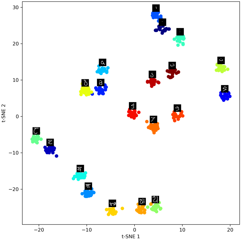
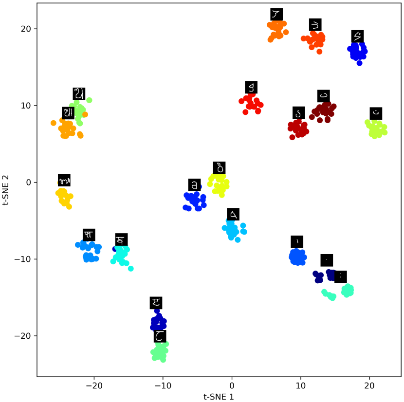
In Fig. 4(a), the t-SNE analysis of the Prototypical Net feature space reveals a strong clustering of the samples belonging to the same class. Note that this phenomenon is not surprising as the loss of the Prototypical Net forces the samples belonging to the same class to be close in the feature space. More surprisingly, we also observe a clustering effect in the SimCLR t-SNE analysis (see Fig. 4(b)). Note that SimCLR is a fully unsupervised algorithm: there is no class information given to the algorithm. Consequently, the strong clustering effect we observe suggests that forcing the proximity between a sample and its augmented version is enough to retrieve the class information. This observation might explain why contrastive learning algorithms are in general so efficient in semi-supervised (or even unsupervised) classification tasks.

S4 Concepts ranked by diversity for the unsupervised setting

Figure S5: Concepts of the Omniglot test set, ranked by their diversity as computed with the unsupervised setting (i.e., SimCLR as a feature extractor and standard deviation for the dispersion measure). Here we linearly sub-sampled $30$ of out of $150$ concepts of the test set. Concepts are ranked in a increasing order (from low to high diversity). The samples in the red box are the prototypes, the rest of the line is composed with samples belonging to the same category.

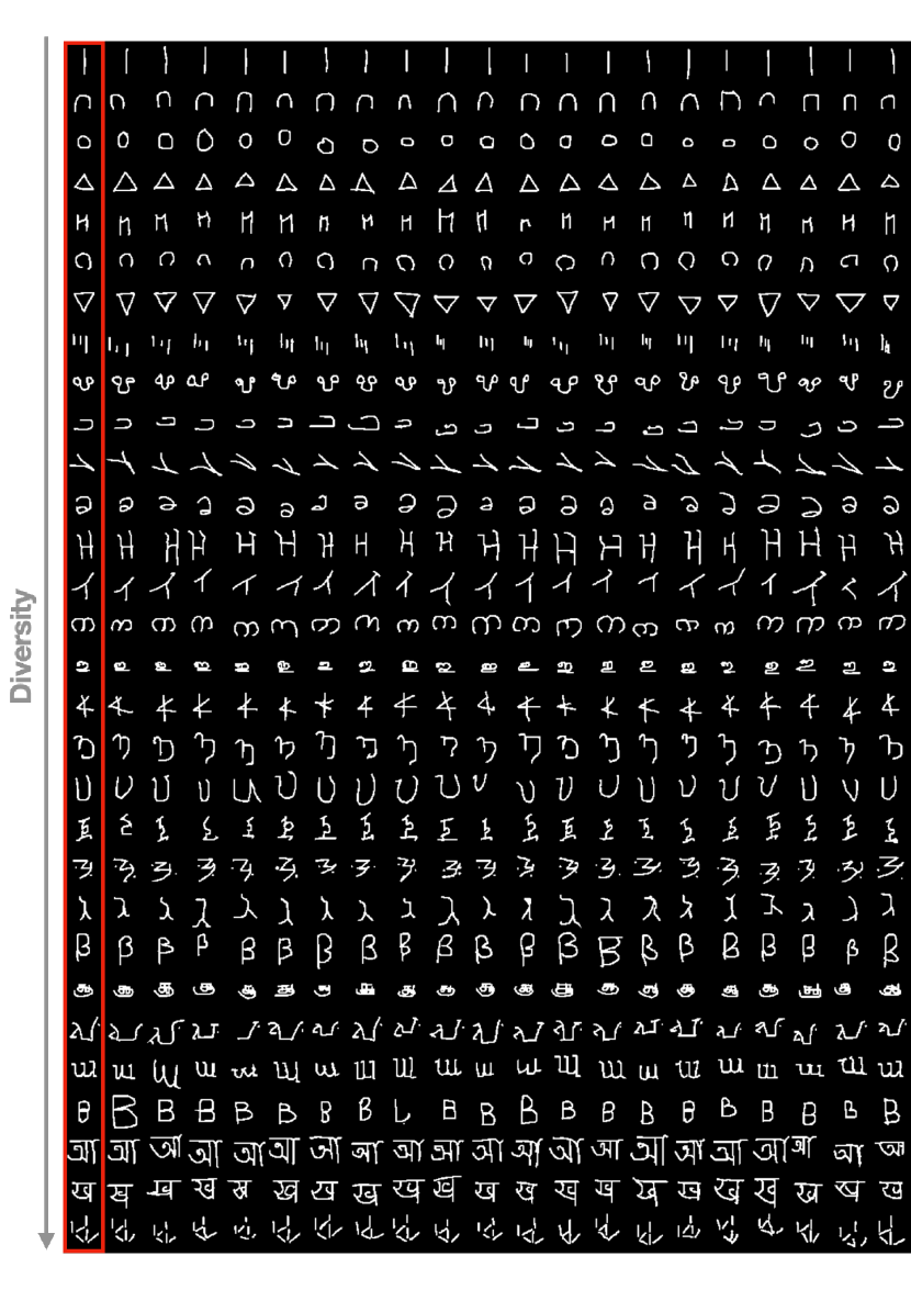
S5 Concepts ranked by diversity for the supervised setting

Figure S6: Concepts of the Omniglot test set, ranked by their diversity as computed with the supervised setting (i.e., Prototypical Net as a feature extractor and standard deviation for the dispersion measure). Here we linearly sub-sampled $30$ of out of $150$ concepts of the test set. Concepts are ranked in a increasing order (from low to high diversity). The samples in the red box are the prototypes, the rest of the line is composed with samples belonging to the same category.

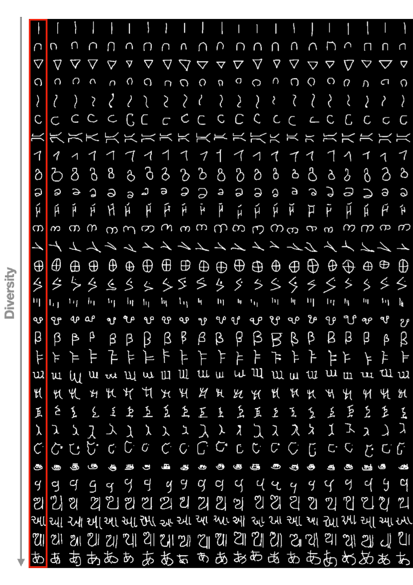
S6 MAML architecture and training details

The architecture we have used for the MAML classifier is exactly the same used for the Prototypical Net (see Table S1). The only difference is the last fully-connected layer that is : Linear(256, 20). Indeed, as the MAML network is directly predicting the logits (and not a distance metric), the last layer needs to have the same dimension than the number of class of the experiment. In a $1$-shot $20$-way classification experiment, the number of classes is $20$.

We have used a $2^{nd}$ order meta-learning scheme [18]. The outer-loop optimizer is an Adam optimizer with a learning rate of $10^{-3}$, and the inner-loop optimizer is a simple Stochastic Gradient Decent with a learning rate of $10^{-2}$. The number of inner loops is set to $5$ during the training and to $10$ during the testing. The number of tasks for each outer-loop is set to $4$.

S7 Control experiments: Comparing Prototypical Net and MAML

To rigorously compare MAML and Prototypical Net, we have conducted $2$ types of control experiments. First we have verified whether the classification accuracy obtained for each class were ranked in the same order for both MAML and Prototypical Net. To do so, we have presented the same series of categorization tasks to both algorithms. The high Spearman rank coefficient ($\rho=0.60$) indicates that both classifiers rank each category’ classification accuracy similarly (see section S4).

To confirm this result, we have computed the correlation between the logits generated by both models. In the case of the MAML model, extracting the logits is straightforward. For Prototypical Net, we use the distance to prototypes as logits. This explain why both model’s logits are anti-correlated: the MAML logits are the (un-normalized) probability of belonging to a given classes whereas the Prototypical Net logits correspond to the distance to the category (so the lower the distance, the higher the probability). We report a strong negative correlation ($r=-0.62$) between the logits of the MAML network and those of Prototypical Net (see section S4).

Table S4: Spearman rank order correlation for different settings

Comparison	correlation type	correlation value	p value
MAML vs. Proto. Net (accuracy)	Spearman	0.60	$4.24\times 10^{-15}$
MAML vs. Proto. Net (logits)	Pearson	-0.62	$2.63\times 10^{-19}$

S8 Architecture and training details of the VAE-STN

S8.1 Architecture of the VAE-STN

The VAE-STN is a sequential VAE that allows for the iterative construction of a complex image [42]. A pseudo-code of the algorithm is described in Algo 1. At each iteration, the algorithm focuses its attention on a specific part of the image ($\boldsymbol{x}$), the prototype ($\boldsymbol{\tilde{x}}$) and the residual image ($\boldsymbol{\hat{x}}$) using the Reading Spatial Transformer Network (STN_r). Then the extracted patch is passed to an encoding network (EncBlock) to transform it into a latent variable. This latent variable is concatenated to a patch extracted from the prototype and then passed to the RecBlock network. The produced hidden state is first passed to DecBlock to recover the original patch, and then to the STN_w to replace and rescale the patch into the original image. The LocNet network is used to learn the parameter of the affine transformation we used in the STN. Note that the affine parameters used in STN_w are simply the inverse of those used in STN_r.

Algorithm 1 Pseudo-code of the VAE-STN

Input: image: x, prototype: $\tilde{\textbf{x}}$

$c\leftarrow\textbf{0}$

$\boldsymbol{\theta_{1}}\leftarrow[[1,0,0],[0,1,0]]$

$\boldsymbol{h_{1}}\leftarrow\boldsymbol{0}$

for $i=1\;\;\text{to}\;\;N_{steps}$ do

     $\boldsymbol{\hat{x}}=\boldsymbol{x}-\text{sigmoid}(\boldsymbol{c})$

     $\boldsymbol{r},\;\boldsymbol{\hat{r}},\;\boldsymbol{\tilde{r}}=STN_{r}(\boldsymbol{\theta_{t}},\boldsymbol{x}),\;STN_{r}(\boldsymbol{\theta_{t}},\boldsymbol{\hat{x}}),\;STN_{r}(\boldsymbol{\theta_{t}},\boldsymbol{\tilde{x}})$

     $\boldsymbol{r}\leftarrow[\boldsymbol{r},\boldsymbol{\hat{r}},\boldsymbol{\tilde{r}},\boldsymbol{h_{t}}]$

     $\boldsymbol{\mu},\boldsymbol{\sigma}=EncBlock(\boldsymbol{r})$

     $\boldsymbol{z}=\boldsymbol{\mu}+\boldsymbol{\epsilon}\boldsymbol{\sigma}\;\;\textrm{with}\;\;\boldsymbol{\epsilon}\sim\mathcal{N}(0,1)$

     $\boldsymbol{z}\leftarrow[\boldsymbol{z},\boldsymbol{\tilde{r}}]$

     $\boldsymbol{p}=DecBlock(\boldsymbol{h_{t}})$

     $\boldsymbol{c}\leftarrow\boldsymbol{c}+STN_{w}(\boldsymbol{\theta_{t}^{-1}},\boldsymbol{p})$

     $\boldsymbol{h_{t+1}}\leftarrow RecBlock(\boldsymbol{z},\boldsymbol{h_{t}})$

     $\boldsymbol{\theta_{t}+1}\leftarrow LocNet(\boldsymbol{h_{t+1}})$

end for

The STN modules take $2$ variables in input: an image (or a patch in the case to the STN_w) and a matrix (3$\times$2) describing the parameters of the affine transformation to apply to the input image [26]. All other modules are made with MLPs networks, and are described in Table S5. In the Table S5 we use the following notations:

• $s_{z}$: This the size of the latent space. In the base architecture, we set $s_{z}=80$.

• $s_{LSTM}$: This is the size of the output of the Long-Short Term Memory (LSTM) unit. In the base architecture, we set $s_{LSTM}=400$

• $s_{r}$: This is the resolution of the patches extracted by the Spatial Transformer Net (STN) during the reading operation. In the base architecture we set $s_{r}=15$.

• $s_{loc}$: This is the number of neurons used at the input of the localization network. In the base architecture, we set $s_{loc}=100$

• $s_{w}$: This is the resolution of the patch passed to the the STN network for the writing operation. In the base architecture $s_{w}=15$.

For the base architecture we used $N_{steps}=60$. The base architecture of the VAE-STN has $6.2$ millions parameters. For more details on the loss function, please refer to [42].

Table S5: Description of the VAE-STN architecture

Network	Layer	# params
EncBlock(sr, sLSTM, sz)	Linear($3$ $\times$ s${}_{r}^{2}$ + sLSTM , $1024$)	($3$ $\times$ s${}_{r}^{2}$ + sLSTM) $\times$ $1024$) + $1024$
	ReLU
	Linear($1024$, $1024$)	$1050$ K
	ReLU
	Linear($1024$, $512$)	$524$ K
	ReLU	-
	Linear($512$, $128$)	$65$ K
	ReLU	-
	Linear($128$, $2\times$ sz)	$256\times$sz + 2$\times$sz
LocNet(sloc)	Linear(sloc, $64$)	s${}_{loc}\times 64$ + $64$
	ReLU	-
	Linear($64$, $32$)	$2$ K
	ReLU	-
	Linear($32$, $6$)	$0.2$ K
DecBlock(sLSTM, sloc, sw)	Linear(sLSTM - sloc, $1024$)	(sLSTM - sloc)$\times 1024$ + $1024$
	ReLU	-
	Linear($1024$, $512$)	$525$ K
	ReLU	-
	Linear($512$, $256$)	$131$ K
	ReLU	-
	Linear($256$, s${}_{w}^{2}$)	$256\times$s${}_{w}^{2}+$s${}_{w}^{2}$
RecBlock(sz, sr, sLSTM)	LSTMCell(sz + s${}_{r}^{2}$, sLSTM)	$4\times\big{(}$sz + s${}_{r}^{2}$)$\times$sLSTM + s${}_{LSTM}^{2}$ + sLSTM)
VAE-STN	EncBlock($15$ , $800$, $80$)	$3,172$ K
	RecBlock($80$, $15$, $800$)	$1,600$ K
	DecBlock($400$, $100$, $15$)	$1,431$ K
	LocNet($100$)	$8.7K$

S8.2 Training details of the VAE-STN

The VAE-STN is trained for $500$ epochs, with batches of size $128$. We use an Adam optimizer with a learning rate of $1\times 10^{-3}$ and $\beta_{1}=0.9$. All other parameters are the default Pytorch parameters. To avoid training instabilities we clip the norm of the gradient to $5$. The learning rate was divided by $2$ when the evaluation loss has not decreased for $10$ epochs (reduce on plateau strategy).

S8.3 VAE-STN samples

Figure S7: Sampled generated by the VAE-STN. All the prototypes used to condition the generative model are in the red frame. The $30$ concepts has been randomly sampled (out of $150$ concepts) from the Omniglot test set. The lines are composed with $20$ samples that has been generated by the VAE-STN.

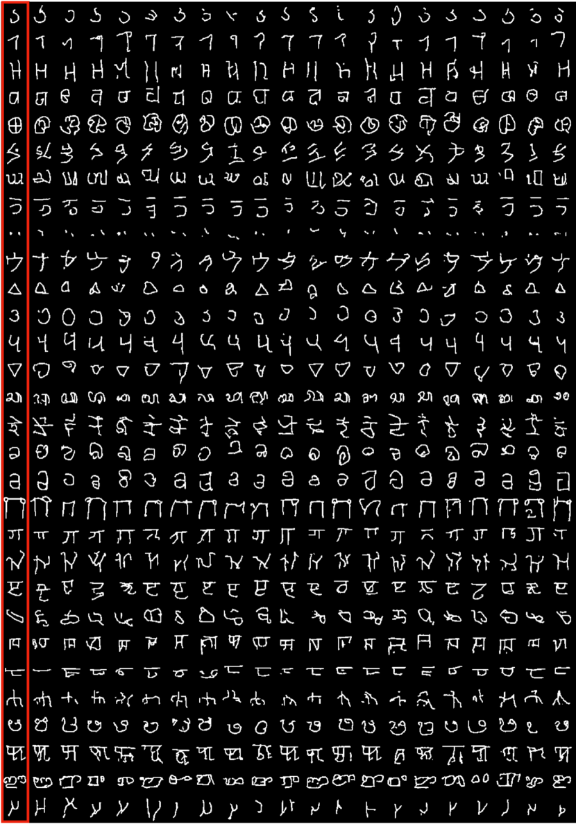
S9 Architecture and training details of the Neural Statistician

Architecture

Figure S8: Left: basic hierarchical model, where the plate encodes the fact that the context variable $c$ is shared across each item in a given dataset. Center: full neural statistician model with three latent layers $z_{1},z_{2},z_{3}$. Each collection of incoming edges to a node is implemented as a neural network, the input of which is the concatenation of the edges’ sources, the output of which is a parameterization of a distribution over the random variable represented by that node. Right: The statistic network, which combines the data via an exchangeable statistic layer. The above figures were obtained from  [15]

Table S6 describes the base architecture of the Neural Statistician model adopted from  [19] which is a close approximation of  [15]. We make minor changes in the network architecture to accommodate the higher input image size of $50\times 50$ of the Omniglot dataset. The Neural Statistician model is composed of the following sub-networks:

• Shared encoder $x\mapsto h$: An instance encoder $E$ that takes each individual datapoint $x_{i}$ to a feature representation $h_{i}$ = $E(x_{i})$.

• Statistic network $q(c|D,\phi):h_{1},...,h_{k}\mapsto\mu_{c},{\sigma^{2}}_{c}$: A pooling layer that aggregates the matrix $(h_{1},...,h_{k})$ to a single pre-statistic vector $v$.  [15] uses sample mean for their experiments. Which is followed by a post-pooling network that takes $v$ to a parametrization of a Gaussian.

• Inference network $q(z|x,c,\phi):h,c\mapsto\mu_{z},{\sigma^{2}}_{z}$: Inference network gives an approximate posterior over latent variables.

• Latent decoder network $p(z|c;\theta):c\mapsto\mu_{z},{\sigma^{2}}_{z}$

• Observation decoder network $p(x|c,z;\theta):c,z\mapsto\mu_{x}$

Table S6: Description of the Neural Statistician Architecture

Network	Layer	# params
ConvBlock(Inc, Outc, stride)	Conv2d(Inc, Outc, stride, 3, padding=1)	Inc $\times$ Outc $\times$ 3 $\times$ 3 + Outc
	BatchNorm2d(Outc), ELU	2 x Outc
FcBlock(In, Out)	Linear(In, Out)	In $\times$ Out
	BatchNorm1d(Out), ELU	-
DeConvBlock(Inc, Outc)	ConvTranspose2d(Inc, Outc, 2, 2)	Inc $\times$ Outc $\times$ 3 $\times$ 3 + Outc
	BatchNorm2d(Outc), ELU	2 x Outc
Shared encoder	ConvBlock(1, 32, 1)	1,958,400
	ConvBlock(32, 32, 1)
	ConvBlock(32, 32, 2)
	ConvBlock(32, 64, 1)
	ConvBlock(64, 64, 1)
	ConvBlock(64, 64, 2)
	ConvBlock(64, 128, 1)
	ConvBlock(128, 128, 1)
	ConvBlock(128, 128, 2)
	ConvBlock(128, 256, 1)
	ConvBlock(256, 256, 1)
	ConvBlock(256, 256, 2)
Statistic network	FcBlock(256*4*4, 256)	1,445,122
	average pooling within each dataset
	2× FcBlock(256, 256)
	Linear(256, 512), BatchNorm1d(1) to $\mu_{c}$, ${\log{\sigma^{2}}_{c}}$
Inference network	FcBlock(256, 256) $\mapsto$ $h$	408,610
	FcBlock(512, 256) $\mapsto$ $c$
	combine c and h, ELU
	Residual Block{3× FcBlock(256, 256)}
	Linear(256, 32), BatchNorm1d(1) to $\mu_{z}$, ${\log{\sigma^{2}}_{z}}$
Latent decoder network	Linear(512, 256) $\mapsto$ $c$, ELU	342,818
	Residual Block{3× FcBlock(256, 256)}
	Linear(256, 32), BatchNorm1d(1) to $\mu_{z}$, ${\log{\sigma^{2}}_{z}}$
Observation decoder network	FcBlock(512, 256) $\mapsto$ $z$	3,324,673
	FcBlock(512, 256) $\mapsto$ $c$
	combine z and c, ELU
	FcBlock(256, 256*4*4)
	ConvBlock(256, 256, 1)
	ConvBlock(256, 256, 1)
	DeConvBlock(256, 256)
	ConvBlock(256, 128, 1)
	ConvBlock(128, 128, 1)
	DeConvBlock(128, 128)
	ConvBlock(128, 64, 1)
	Conv2d(64, 64, 4, 1, 0)
	DeConvBlock(64, 64)
	ConvBlock(64, 32, 1)
	Conv2d(32, 32, 2, 1, 0)
	DeConvBlock(32, 32)
	Conv2d(32, 1, 1)

The overall number of parameters of the base model (which has the same architecture as used in  [15]) for the Neural Statistician we are using is around 7.48M parameters.

Training details

The Neural Statistician is trained for 300 epochs, with batch size of 32 and learning rate of $1\times 10^{-3}$. We adopt the same setting of the Neural Statistician as used in  [15] for the omniglot dataset. We constructed context sets by splitting each class into datasets of size 5 while training, and use a single out-of-distribution exemplar while testing. As discussed in the paper, we create new classes by reflecting and rotating characters. We based our implementation from https://github.com/georgosgeorgos/hierarchical-few-shot-generative-models and https://github.com/comRamona/Neural-Statistician.

Intuition about context integration in the Neural-Statistician

In the Neural Statistician, the context correspond to the samples used during training, to evaluate the statistics of a specific category (i.e. a concept). In practice, we pass to the network different samples representing the same concept and we vary the number of these samples (from $2$ to $20$ in the experiment described in section 4.2). Intuitively, with more context samples for a given category, it becomes easier for the network to identify the properties and features that are crucial to define a given handwritten letter (which results in a higher recognizability but leaves less room for diversity).

S9.1 Neural statistician samples

Figure S9: Sampled generated by the neural statistician network (VAE-NS). All the prototypes used to condition the generative model are in the red frame. The $30$ concepts has been randomly sampled (out of $150$ concepts) from the Omniglot test set. The lines are composed with $20$ samples that has been generated by the VAE-NS.

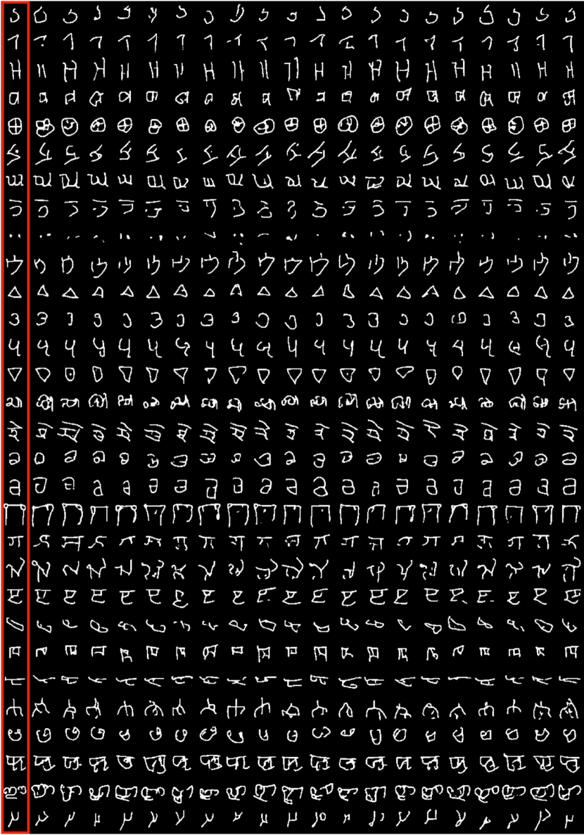
S10 Architecture and training details of the DA-GAN based on U-Net (DA-GAN-UN)

Architecture

Figure S10: DAGAN Generator: The generator is composed of an encoder projecting the input image to a lower dimensional manifold. A random gaussian noise vector is transformed and concatenated with the bottleneck vector. The resulting vector is passed through the decoder (generator), which outputs the augmented image.

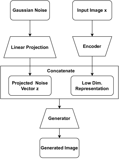
Table S7 describes the base architecture of the DA-GAN-UN’s Generator model adopted from  [1]. We have modified the architecture of the DA-GAN-UN model such that it can accommodate a higher input image size $50\times 50$. Also, we reduced the number of trainable parameters in the original DA-GAN-UN architecture to have a fair comparison with other few-shot models. Following are the notations used in Table S7:

• s_z: This is the size of the latent space. In the base architecture, we set s_z = 128

• Generator $G(x,z)$: A generator network that takes data points and Gaussian noise as input, and generate new samples.

The base architecture of the DAGAN model we are using in our experiments has around 6.8 million parameters.

Training details

The DA-GAN-UN model was trained for 30 epochs, with batches of size 32. We use an Adam optimizer with a learning rate of 1 $\times 10^{-4}$ and $\beta_{1}$ = 0.9. We update our generator after every 5 updates of discriminator. We based our implementation from https://github.com/amurthy1/dagan_torch

Table S7: Description of the Data Augmentation GAN Architecture

Network	Layer	# params
ConvBlock(Inc, Outc, sl)	Conv2d(Inc, Outc, 3, stride=sl, padding=1)	Outc $\times$ (Inc $\times$ 3 $\times$ 3 + 1)
	LeakyReLU(0.2), BatchNorm2d(Outc)	2 x Outc
DeConvBlock(Inc, Outc, sl)	ConvTranspose2d(Inc, Outc, 3, stride=sl, padding=1)	Outc $\times$ (Inc $\times$ 3 $\times$ 3 + 1)
	LeakyReLU(0.2), BatchNorm2d(Outc)	2 x Outc
EncoderBlock(Inp, Inc, Outc)	ConvBlock(Inp, Inp)
	ConvBlock(Inc + Inp, Outc)
	Conv2d(Inc+ Outc, Outc)
	Conv2d(Inc+ 2 $\times$ Outc, Outc)
DecoderBlock(Inp, Inc, Outc)	DeConvBlock(Inp, Inp, 1)
	ConvBlock(Inc+Inp, Outc, 1)
	DeConvBlock(Inp, Inp, 1)
	ConvBlock(Inc + Inp + Outc, Outc, 1)
	DeConvBlock(Inc + 2 $\times$ Outc, Outc, 1)
Generator(sz)	ConvBlock(1, 64, 2)	6,813,857
	EncoderBlock(1, 64, 64)
	EncoderBlock(64, 64, 128)
	EncoderBlock(128, 128, 128)
	Linear(sz, 4$\times$4$\times$8)
	DecoderBlock(0, 136, 64)
	Linear(sz, 7$\times$7$\times$4)
	DecoderBlock(128, 260, 64)
	Linear(sz, 13$\times$13$\times$2)
	DecoderBlock(128, 194, 64)
	DecoderBlock(64, 128, 64)
	DecoderBlock(64, 65, 64)
	ConvBlock(64, 64, 1)
	ConvBlock(64, 64, 1)
	Conv2d(64, 1, 3, stride=1, padding=1)

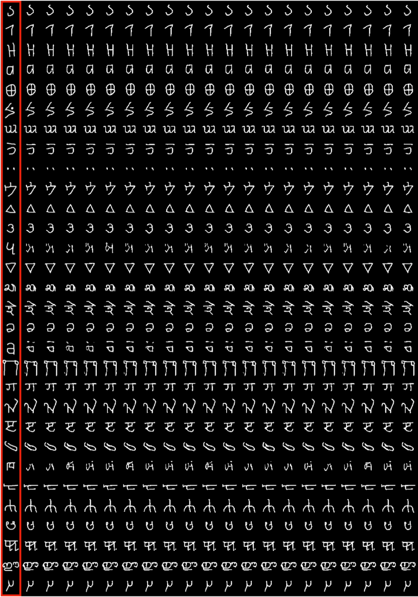
S10.1 DA-GAN-UN samples

Figure S11: Sampled generated by the Data Augmentation GAN with U-Net architecture (DA-GAN-UN). All the prototypes used to condition the generative model are in the red frame. The $30$ concepts has been randomly sampled (out of $150$ concepts) from the Omniglot test set. The lines are composed with $20$ samples that has been generated by the DA-GAN-UN.

S11 Architecture and training details of the DA-GAN based on ResNet (DA-GAN-RN)

Architecture

We use the same base architecture of DA-GAN-UN, except we remove the skip connections between the contracting path (encoder) and the expansive path (decoder).  [1] used a combination of UNet and ResNet in their results, in DA-GAN-RN we consider only a ResNet type architecture.

Training details

Refer  S10 for training details.

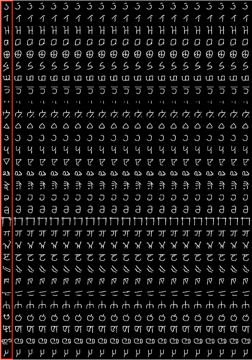
S11.1 DA-GAN-RN samples

Figure S12: Sampled generated by the Data Augmentation GAN with ResNet architecture (DA-GAN-RN). All the prototypes used to condition the generative model are in the red frame. The $30$ concepts has been randomly sampled (out of $150$ concepts) from the Omniglot test set. The lines are composed with $20$ samples that has been generated by the DA-GAN-RN.

S12 Effect of the number of context samples on the diversity/recognizability framework

Figure S13: Effect of the number of context samples on the diversity/recognizability framework for $3$ different runs. (a) Effect of the number of context samples on the diversity. (b) Effect of the number of context samples on the recognizability. (c) Simultaneous evolution of diversity and recognizability when ones varies the number of context samples from $2$ to $20$.

We observe a monotonic decrease of the diversity and a monotonic increase of the recognizability when the number of context samples increases. We vary the number of context samples from $2$ to $20$. This experiment has been conducted with $3$ different seeds (i.e., different network initialization), represented with red, green and blue data points, respectively. For each seed, we report $19$ data points. To highlight the trend in the diversity-recognizability space, we have smoothed the curves in Fig. S13a and Fig. S13b, using a Savitzky-Golay filter (second order, window size of 7).

S13 Effect of the number of attentional steps on the diversity/recognizability framework

Figure S14: Effect of the number of attentional steps on the diversity/recognizability framework for $3$ different runs. (a) Effect of the number of attentional steps on the diversity. (b) Effect of the number of attentional steps on the recognizability. (c) Simultaneous evolution of diversity and recognizability when one varies the number of attentional steps from $20$ to $90$

In this experiment, we have varied the number of attentional steps from $20$ to $90$. Note that we could not go below $20$ attentional steps to make sure the attentional process is fully covering the entire image. We did not go over $90$ attentional steps because we faced some training instabilities beyond this point. We observe a non-monotonic evolution of the diversity and the recognizability with the increase of the number of attentional steps. This experiment has been conducted with $3$ different seeds (i.e., different network initialization), represented with red, green and blue data points, respectively. For each seed we report $8$ data points. In order to properly assess the type of parametric curves that govern the evolution of the diversity-recognizability space when one varies the number of attentional steps, we have used a least curve fitting method [21]. This method involves finding the best polynomial fit (second order in our case) for the $3$ curves (Fig. S14a, b and c) simultaneously. This method is iteratively refining all the fits to minimize the sum of all least square error.

S14 Mathematical formulation of the ELBO

Let us consider a dataset $\boldsymbol{X}=\{\boldsymbol{x^{(i)}}\}_{i=1}^{N}$ composed of $N$ i.i.d samples of a random variable $\boldsymbol{x}$. We assume that $\boldsymbol{x}$ is generated by some random process involving an unobserved random variable $\boldsymbol{z}$. The latent variable $\boldsymbol{z}$ is sampled from a Gaussian distribution (see Eq. 5). The mean of the likelihood is parametrized by $\boldsymbol{\mu}_{\theta}$ (in which $\theta$ denotes the parameters) and its variance is considered constant.

$$\boldsymbol{x}\sim p_{\theta}(\boldsymbol{x}\mid\boldsymbol{z})\quad \mbox{s.t}\quad p_{\theta}(\boldsymbol{x}\mid\boldsymbol{z})=\mathcal{N}\big{(}\boldsymbol{x};\boldsymbol{\mu}_{\theta}(\boldsymbol{z}),\boldsymbol{\sigma}^{2}_{x}\big{)}$$ (4)

$$\boldsymbol{z}\sim p(\boldsymbol{z})\quad \mbox{s.t}\quad p(\boldsymbol{z})=\mathcal{N}\big{(}\boldsymbol{z};\boldsymbol{\mu}_{p},\boldsymbol{\sigma}^{2}_{p}\big{)}$$ (5)

The Variational Auto Encoder is optimized by maximizing the Evidence Lower Bound (ELBO), as formalized in its simplest form in Eq. 6:

$$ELBO(\boldsymbol{x},\theta,\phi) =\mathbb{E}_{q_{\phi}(\boldsymbol{z}\mid\boldsymbol{x})}[\log p_{\theta}(\boldsymbol{x}\mid\boldsymbol{z})]-\beta\operatorname*{KL}\big{(}q_{\phi}(\boldsymbol{z}\mid\boldsymbol{x})\lVert p(\boldsymbol{z})\big{)}$$ (6)

One could observe that the $\beta$ coefficient is tuning the importance of the prior (through the KL). If $\beta>1$, then the latent space will be forced to be closer to the prior distribution but will attenuate the weight of the reconstruction loss. Such a scenario tends to improve the disentanglement of the latent space [24]. On the contrary, if $\beta$ is low, then the reconstruction loss (i.e., $\mathbb{E}_{q_{\phi}(\boldsymbol{z}\mid\boldsymbol{x})}[\log p_{\theta}(\boldsymbol{x}\mid\boldsymbol{z})]$) will take over, and then the latent space will be less regularized. Note that in the extreme case where $\beta=0$, the VAE becomes an auto-encoder.

The ELBO loss can be updated to include a latent variable encoding for the context $\boldsymbol{c}$ as in the VAE-NS. In this formulation, the context corresponds to a dataset $D$ (see Eq. 7):

$$ELBO(\boldsymbol{x},\theta,\phi) =\mathbb{E}_{q_{\phi}(\boldsymbol{c}\mid D)}\Big{[}\sum_{\boldsymbol{x}\in D}\mathbb{E}_{q_{\phi}(\boldsymbol{z}\mid\boldsymbol{c},\boldsymbol{x})}[\log p_{\theta}(\boldsymbol{x}\mid\boldsymbol{z})]-\beta\operatorname*{KL}\big{(}q_{\phi}(\boldsymbol{z}\mid\boldsymbol{c},\boldsymbol{x})\lVert p(\boldsymbol{z}\mid\boldsymbol{c})\big{)}\Big{]}$$ (7)

$$-\operatorname*{KL}\big{(}q_{\phi}(\boldsymbol{z}\mid D)\lVert p(\boldsymbol{c})\big{)}$$

The ELBO could also be extended to include a sequential generative process as in the VAE-STN. In this case, the latent variable $\boldsymbol{z}$ is time-indexed and is now a sequence of random variables denoted $(\boldsymbol{z_{1}},..,\boldsymbol{z_{T}})$. In Eq. 8, $\boldsymbol{z_{<k}}$ indicates the collection of all latent variables from step $t=1$ to $t=k$.

$$ELBO(\boldsymbol{x},\theta,\phi) =\mathbb{E}_{q_{\phi}(\boldsymbol{z_{1}},..,\boldsymbol{z_{T}}\mid\boldsymbol{x})}[\log p_{\theta}(\boldsymbol{x}\mid\boldsymbol{z_{1}},..,\boldsymbol{z_{T}})]-\beta\operatorname*{KL}\sum_{k=1}^{T}\big{(}q_{\phi}(\boldsymbol{z_{k}}\mid\boldsymbol{z_{<k}},\boldsymbol{x})\lVert p(\boldsymbol{z_{k}})\big{)}$$ (8)

S15 Effect of the beta coefficient on the diversity/recognizability framework

In this experiment, we have varied the value of the $\beta$ coefficient from $0.25$ to $4$ for the VAE-STN and from $0.25$ to $5$ for VAE-NS model. This experiment has been conducted with $3$ different seeds (i.e., different network initialization), represented with red, green and blue data points, respectively. For the VAE-STN and for each seed, we have collected $16$ data points (see Fig. S15), and $20$ for the VAE-NS (see Fig. S16). We use a similar method than in S13 to find a polynomial fit (second order in our case) of the curves shown in Fig. S15a, b, and c and Fig. S16a, b, and c. We report a quasi-monotonic decline of the diversity when the beta value is increased (see Fig. S15a and Fig. S16a). In contrast, the recognizability follows a parabolic relationship when the beta value is increased. For the VAE-STN, the maximum recognizability ($\approx 80\%$) is reached for a $\beta$ value of $2.25$ (see Fig. S15b). For the VAE-NS, the maximum recognizability ($\approx 91\%$) is reached for a $\beta$ value of $3$ (see Fig. S16b). Even if the change of amplitude in recognizability and in diversity is larger for the VAE-STN than for VAE-NS, the shapes of the curves are very similar.

Figure S15: Effect of varying $\beta$ in the VAE-STN on the diversity/recognizability framework for $3$ different runs. (a) Effect of $\beta$ on the diversity. (b) Effect of $\beta$ on the recognizability. (c) Parametric curve recognizability versus diversity when one varies $\beta$ from $0.25$ from to $4$.

Figure S16: Effect of varying $\beta$ in the VAE-NS on the diversity/recognizability framework for $3$ different runs. (a) Effect of $\beta$ on the diversity. (b) Effect of $\beta$ on the recognizability. (c) Parametric curve recognizability versus diversity when one varies $\beta$ from $0.25$ from to $5$.

S16 Effect of the size of the latent space on the diversity/recognizability framework

Figure S17: Effect of varying the size of the latent vector ($z$) in the VAE-NS on the diversity/recognizability framework for $3$ different runs. (a) Effect of latent size on the diversity. (b) Effect of the latent size on the recognizability. (c) Parametric curve recognizability versus diversity when one varies $\beta$ from $5$ from to $100$.

Figure S18: Effect of varying the size of the latent vector ($z$) in the VAE-STN on the diversity/recognizability framework for $3$ different runs. (a) Effect of latent size on the diversity. (b) Effect of the latent size on the recognizability. (c) Parametric curve recognizability versus diversity when one varies $\beta$ from $5$ from to $400$.

Figure S19: Effect of varying the size of the latent vector ($z$) in the DA-GAN-UN on the diversity/recognizability framework for $3$ different runs. (a) Effect of latent size on the diversity. (b) Effect of the latent size on the recognizability. (c) Parametric curve recognizability versus diversity when one varies $\beta$ from $10$ from to $1000$.

Figure S20: Effect of varying the size of the latent vector ($z$) in the DA-GAN-RN on the diversity/recognizability framework for $3$ different runs. (a) Effect of latent size on the diversity. (b) Effect of the latent size on the recognizability. (c) Parametric curve recognizability versus diversity when one varies $\beta$ from $10$ from to $500$.

S17 Overfitting of standard classifier in low-data regime

Omniglot is a dataset composed of images representing 1,623 classes of handwritten letters and symbols (extracted from 50 different alphabets) with just 20 samples per class. This low number of samples per class makes Omniglot very different from other datasets (e.g. MNIST, CIFAR10…). In such a low-data regime, standard deep learning classifiers are known to overfit to the training data [7] resulting in poor generalization performance. In this section we provide experimental confirmation of such a phenomenon.

We have trained 3 different classifiers, all having a similar architecture (the architecture is described in Table S1):

• A standard classifier. For this classifier, the last linear layer has been changed to have an output activation of size $1623$. Said differently, the layer entitled "Linear(256, 128)" in Table S1 has been replaced by "Linear(256, 1623)". We have trained this classifier using $18$ samples per class of the Omniglot dataset. The testing set is composed of the $2$ remaining samples per class. To summarize, the training set is composed of $29,214$ samples ($1623\times 18$) and the training set is composed of $3246$ samples ($1623\times 2$). This classifier is trained using a standard back-propagation on a cross-entropy loss (same learning parameters than those described in Section S1). Train/test loss and classification accuracy are reported for all training epochs in Fig S21a and Fig S21d, respectively.

• A one-shot classifier. Both the architecture and the training procedure of this classifier are described in Section S1. We remind the reader that we use a weak generalization split to train the few-learning networks (i.e. $1473$ classes in the training set and $150$ classes of testing set). Train/test loss and classification accuracy are reported for all training epochs in Fig S21b and Fig S21e, respectively.

• A five-shot classifier. This network is the exact same than the one-shot Prototypical Net described before, except that it is trained in a 5-shots settings. Train/test loss and classification accuracy are reported for all training epochs in Fig S21c and Fig S21f, respectively.

Figure S21: Comparison between different classifiers in low-data regime. Train and test losses at each training epoch for (a) a standard classifier, (b) a Protypical Net in a one-shot learning setting and (c) a Prototypical Net in a 5-shots learning setting. Train and test classification accuracy at each training epoch for (d) a standard classifier, (e) a Protypical Net in a one-shot learning setting and (f) a Prototypical Net in a 5-shots learning setting.

For the standard classifier, we observe an increase of the test loss (resp. a decrease of the test accuracy) while the train loss is still decreasing (resp. the train accuracy is still increasing), see Fig S21a and Fig S21d. It suggests that the network becomes better at classifying the training samples but worst at dealing with the testing samples. The standard classifier is then overfitting on the training set. Note that the $2$ other few-shots learning networks are not showing such a decrease in the test loss and accuracy. Such an experiment suggests that standard classifiers are not adequate to extract features of samples in a low-data regime.

S18 Computational Resources

All the experiments of this paper have been performed using Tesla V100 with 16 Gb memory. The training time is dependent on the hyper-parameters, but varies between 4h to 24h per simulation.

S19 Broader Impact

This work does not present any foreseeable negative societal consequences. We think the societal impact of this work is positive. It might help the neuroscience community to evaluate the different mechanisms that allow human-level generalization, and then better understand the brain.

References

- Antoniou et al. [2017] Antoniou Antreas, Storkey Amos, Edwards Harrison. Data augmentation generative adversarial networks // arXiv preprint arXiv:1711.04340. 2017.
- Arjovsky et al. [2017] Arjovsky Martin, Chintala Soumith, Bottou Léon. Wasserstein generative adversarial networks // International conference on machine learning. 2017. 214–223.
- Barratt, Sharma [2018] Barratt Shane, Sharma Rishi. A note on the inception score // arXiv preprint arXiv:1801.01973. 2018.
- Bishop, Nasrabadi [2006] Bishop Christopher M, Nasrabadi Nasser M. Pattern recognition and machine learning. 4, 4. 2006.
- Boutin et al. [2020a] Boutin Victor, Franciosini Angelo, Ruffier Franck, Perrinet Laurent. Effect of top-down connections in Hierarchical Sparse Coding // Neural Computation. 2020a. 32, 11. 2279–2309.
- Boutin et al. [2020b] Boutin Victor, Zerroug Aimen, Jung Minju, Serre Thomas. Iterative VAE as a predictive brain model for out-of-distribution generalization // arXiv preprint arXiv:2012.00557. 2020b.
- Brigato, Iocchi [2021] Brigato Lorenzo, Iocchi Luca. A close look at deep learning with small data // 2020 25th International Conference on Pattern Recognition (ICPR). 2021. 2490–2497.
- Broedelet et al. [2022] Broedelet Iris, Boersma Paul, Rispens Judith, others . School-Aged Children Learn Novel Categories on the Basis of Distributional Information // Frontiers in Psychology. 2022. 12, 799241.
- Burgess et al. [2018] Burgess Christopher P, Higgins Irina, Pal Arka, Matthey Loic, Watters Nick, Desjardins Guillaume, Lerchner Alexander. Understanding disentangling in beta-VAE // arXiv preprint arXiv:1804.03599. 2018.
- Chen et al. [2020] Chen Ting, Kornblith Simon, Norouzi Mohammad, Hinton Geoffrey. A simple framework for contrastive learning of visual representations // International conference on machine learning. 2020. 1597–1607.
- Choksi et al. [2021] Choksi Bhavin, Mozafari Milad, Biggs O’May Callum, Ador Benjamin, Alamia Andrea, VanRullen Rufin. Predify: Augmenting deep neural networks with brain-inspired predictive coding dynamics // Advances in Neural Information Processing Systems. 2021. 34.
- Chomsky [1965] Chomsky Noam. Aspects of the theory of syntax Special technical report no. 11. 1965.
- Chong, Forsyth [2020] Chong Min Jin, Forsyth David. Effectively unbiased fid and inception score and where to find them // Proceedings of the IEEE/CVF conference on computer vision and pattern recognition. 2020. 6070–6079.
- Chowdhury et al. [2022] Chowdhury Arkabandhu, Chaudhari Dipak, Chaudhuri Swarat, Jermaine Chris. Meta-Meta Classification for One-Shot Learning // Proceedings of the IEEE/CVF Winter Conference on Applications of Computer Vision. 2022. 177–186.
- Edwards, Storkey [2016] Edwards Harrison, Storkey Amos. Towards a neural statistician // arXiv preprint arXiv:1606.02185. 2016.
- Feinman, Lake [2020] Feinman Reuben, Lake Brenden M. Generating new concepts with hybrid neuro-symbolic models // arXiv preprint arXiv:2003.08978. 2020.
- Feldman [1997] Feldman Jacob. The structure of perceptual categories // Journal of mathematical psychology. 1997. 41, 2. 145–170.
- Finn et al. [2017] Finn Chelsea, Abbeel Pieter, Levine Sergey. Model-agnostic meta-learning for fast adaptation of deep networks // International conference on machine learning. 2017. 1126–1135.
- Giannone, Winther [2021] Giannone Giorgio, Winther Ole. Hierarchical Few-Shot Generative Models // Fifth Workshop on Meta-Learning at the Conference on Neural Information Processing Systems. 2021.
- Goodfellow et al. [2014] Goodfellow Ian, Pouget-Abadie Jean, Mirza Mehdi, Xu Bing, Warde-Farley David, Ozair Sherjil, Courville Aaron, Bengio Yoshua. Generative adversarial nets // Advances in neural information processing systems. 2014. 27.
- Grossman [1971] Grossman M. Parametric curve fitting // The Computer Journal. 1971. 14, 2. 169–172.
- Heusel et al. [2017] Heusel Martin, Ramsauer Hubert, Unterthiner Thomas, Nessler Bernhard, Hochreiter Sepp. Gans trained by a two time-scale update rule converge to a local nash equilibrium // Advances in neural information processing systems. 2017. 30.
- Higgins et al. [2021] Higgins Irina, Chang Le, Langston Victoria, Hassabis Demis, Summerfield Christopher, Tsao Doris, Botvinick Matthew. Unsupervised deep learning identifies semantic disentanglement in single inferotemporal face patch neurons // Nature communications. 2021. 12, 1. 1–14.
- Higgins et al. [2016] Higgins Irina, Matthey Loic, Pal Arka, Burgess Christopher, Glorot Xavier, Botvinick Matthew, Mohamed Shakir, Lerchner Alexander. beta-vae: Learning basic visual concepts with a constrained variational framework // arXiv preprint arXiv:1804.03599. 2016.
- Hinton et al. [2012] Hinton Geoffrey, Srivastava Nitish, Swersky Kevin. Neural networks for machine learning lecture 6a overview of mini-batch gradient descent // Cited on. 2012. 14, 8. 2.
- Jaderberg et al. [2015] Jaderberg Max, Simonyan Karen, Zisserman Andrew, others . Spatial transformer networks // Advances in neural information processing systems. 2015. 28.
- Jongejan et al. [2016] Jongejan Jonas, Rowley Henry, Kawashima Takashi, Kim Jongmin, Fox-Gieg Nick. The quick, draw!-ai experiment // Mount View, CA, accessed Feb. 2016. 17, 2018. 4.
- Kingma, Ba [2014] Kingma Diederik P, Ba Jimmy. Adam: A method for stochastic optimization // arXiv preprint arXiv:1412.6980. 2014.
- Kingma, Welling [2013] Kingma Diederik P, Welling Max. Auto-encoding variational bayes // arXiv preprint arXiv:1312.6114. 2013.
- Kingma, Dhariwal [2018] Kingma Durk P, Dhariwal Prafulla. Glow: Generative flow with invertible 1x1 convolutions // Advances in neural information processing systems. 2018. 31.
- Koch et al. [2015] Koch Gregory, Zemel Richard, Salakhutdinov Ruslan, others . Siamese neural networks for one-shot image recognition // ICML deep learning workshop. 2. 2015. 0.
- Lake et al. [2015] Lake Brenden M, Salakhutdinov Ruslan, Tenenbaum Joshua B. Human-level concept learning through probabilistic program induction // Science. 2015. 350, 6266. 1332–1338.
- Lake et al. [2017] Lake Brenden M, Ullman Tomer D, Tenenbaum Joshua B, Gershman Samuel J. Building machines that learn and think like people // Behavioral and brain sciences. 2017. 40.
- Larsen et al. [2016] Larsen Anders Boesen Lindbo, Sønderby Søren Kaae, Larochelle Hugo, Winther Ole. Autoencoding beyond pixels using a learned similarity metric // International conference on machine learning. 2016. 1558–1566.
- Li et al. [2021] Li Xiaoxu, Yang Xiaochen, Ma Zhanyu, Xue Jing-Hao. Deep metric learning for few-shot image classification: A selective review // arXiv preprint arXiv:2105.08149. 2021.
- Lucas et al. [2019] Lucas Thomas, Shmelkov Konstantin, Alahari Karteek, Schmid Cordelia, Verbeek Jakob. Adaptive density estimation for generative models // Advances in Neural Information Processing Systems. 2019. 32.
- Mishra et al. [2017] Mishra Nikhil, Rohaninejad Mostafa, Chen Xi, Abbeel Pieter. A simple neural attentive meta-learner // arXiv preprint arXiv:1707.03141. 2017.
- Nalisnick et al. [2018] Nalisnick Eric, Matsukawa Akihiro, Teh Yee Whye, Gorur Dilan, Lakshminarayanan Balaji. Do deep generative models know what they don’t know? // arXiv preprint arXiv:1810.09136. 2018.
- Oord Van den et al. [2016] Oord Aaron Van den, Kalchbrenner Nal, Espeholt Lasse, Vinyals Oriol, Graves Alex, others . Conditional image generation with pixelcnn decoders // Advances in neural information processing systems. 2016. 29.
- Piattelli-Palmarini [1980] Piattelli-Palmarini Massimo. Language and learning: the debate between Jean Piaget and Noam Chomsky // Harvard Univ Press, Cambridge, MA. 1980.
- Rao, Ballard [1999] Rao Rajesh PN, Ballard Dana H. Predictive coding in the visual cortex: a functional interpretation of some extra-classical receptive-field effects // Nature neuroscience. 1999. 2, 1. 79–87.
- Rezende et al. [2016] Rezende Danilo, Danihelka Ivo, Gregor Karol, Wierstra Daan, others . One-shot generalization in deep generative models // International conference on machine learning. 2016. 1521–1529.
- Richards et al. [1992] Richards Whitman, Feldman Jacob, Jepson A. From features to perceptual categories // BMVC92. 1992. 99–108.
- Salakhutdinov et al. [2012] Salakhutdinov Ruslan, Tenenbaum Joshua, Torralba Antonio. One-shot learning with a hierarchical nonparametric bayesian model // Proceedings of ICML Workshop on Unsupervised and Transfer Learning. 2012. 195–206.
- Salimans et al. [2016] Salimans Tim, Goodfellow Ian, Zaremba Wojciech, Cheung Vicki, Radford Alec, Chen Xi. Improved techniques for training gans // Advances in neural information processing systems. 2016. 29.
- Santoro et al. [2016] Santoro Adam, Bartunov Sergey, Botvinick Matthew, Wierstra Daan, Lillicrap Timothy. Meta-learning with memory-augmented neural networks // International conference on machine learning. 2016. 1842–1850.
- Snell et al. [2017] Snell Jake, Swersky Kevin, Zemel Richard. Prototypical networks for few-shot learning // Advances in neural information processing systems. 2017. 30.
- Sung et al. [2018] Sung Flood, Yang Yongxin, Zhang Li, Xiang Tao, Torr Philip HS, Hospedales Timothy M. Learning to compare: Relation network for few-shot learning // Proceedings of the IEEE conference on computer vision and pattern recognition. 2018. 1199–1208.
- Szegedy et al. [2016] Szegedy Christian, Vanhoucke Vincent, Ioffe Sergey, Shlens Jon, Wojna Zbigniew. Rethinking the inception architecture for computer vision // Proceedings of the IEEE conference on computer vision and pattern recognition. 2016. 2818–2826.
- Taylor, Ivry [2013] Taylor Jordan A, Ivry Richard B. Context-dependent generalization // Frontiers in Human Neuroscience. 2013. 7. 171.
- Tenenbaum [1998] Tenenbaum Joshua. Bayesian modeling of human concept learning // Advances in neural information processing systems. 1998. 11.
- Tiedemann et al. [2021] Tiedemann Henning, Morgenstern Yaniv, Schmidt Filipp, Fleming Roland W. One shot generalization in humans revealed through a drawing task // bioRxiv. 2021.
- Van Den Oord et al. [2017] Van Den Oord Aaron, Vinyals Oriol, others . Neural discrete representation learning // Advances in neural information processing systems. 2017. 30.
- Wyatte et al. [2012] Wyatte Dean, Curran Tim, O’Reilly Randall. The limits of feedforward vision: Recurrent processing promotes robust object recognition when objects are degraded // Journal of Cognitive Neuroscience. 2012. 24, 11. 2248–2261.