\IEEEoverridecommandlockouts\overrideIEEEmargins

Online Optimization of Dynamical Systems With Deep Learning Perception

 Liliaokeawawa Cothren\affilmark1    Gianluca Bianchin\affilmark1    Emiliano Dall’Anese\affilmark1 Department of Electrical, Computer, and Energy Engineering, University of Colorado Boulder, Boulder, CO, USA
Abstract

This paper considers the problem of controlling a dynamical system when the state cannot be directly measured and the control performance metrics are unknown or partially known. In particular, we focus on the design of data-driven controllers to regulate a dynamical system to the solution of a constrained convex optimization problem where: i) the state must be estimated from nonlinear and possibly high-dimensional data; and, ii) the cost of the optimization problem – which models control objectives associated with inputs and states of the system – is not available and must be learned from data. We propose a data-driven feedback controller that is based on adaptations of a projected gradient-flow method; the controller includes neural networks as integral components for the estimation of the unknown functions. Leveraging stability theory for perturbed systems, we derive sufficient conditions to guarantee exponential input-to-state stability (ISS) of the control loop. In particular, we show that the interconnected system is ISS with respect to the approximation errors of the neural network and unknown disturbances affecting the system. The transient bounds combine the universal approximation property of deep neural networks with the ISS characterization. Illustrative numerical results are presented in the context of robotics and control of epidemics.

{IEEEkeywords}

Optimization, Gradient methods, Neural networks, Regulation, Perception-based control.

1 Introduction

Control frameworks for modern engineering and societal systems critically rely on the use of perceptual information from sensing and estimation mechanisms. Extraction of critical information for feedback control increasingly requires the processing of high-dimensional sensory data obtained from nonlinear sensory systems [1, 2, 3, 4], and the interpretation of information received from humans interacting with the system regarding the end-user perception of safety, comfort, or (dis)satisfaction [5, 6]. For example, control systems in autonomous driving rely on positioning information extracted from camera images [1] and must account for the perception of the safety of the vehicle occupants [7]. In power grids, state feedback is derived from nonlinear state estimators or pseudo-measurements [8], and control goals must account for comfort and satisfaction objectives of the end-users that are difficult to model [9].

Within this broad context, this paper considers the problem of developing feedback controllers for dynamical systems where the acquisition of information on the system state and on the control performance metrics requires a systematic integration of supervised learning methods in the controller design process. The particular problem that is tackled in this paper pertains to the design of feedback controllers to steer a dynamical system toward the solution of a constrained convex optimization problem, where the cost models objectives are associated with the state and the controllable inputs. The design of feedback controllers inspired by first-order optimization methods has received significant attention during the last decade [10, 11, 12, 13, 14, 15, 16, 17, 18, 19]; see also the recent line of work on using online optimization methods for discrete-time linear time-invariant (LTI) systems [20, 21, 22, 23]. However, open research questions remain on how it is possible to systematically integrate learning methods in the control loop when information on the system and on the optimization model is not directly available, and on how to analyze the robustness and safety of optimization-based controllers in the presence of learning errors.

In this work, we investigate the design of feedback controllers, based on an adaptation of the projected gradient flow method [24, 18], combined with learning components where: i) estimates of the state of the system are provided by feedforward neural networks [25, 26] and residual neural networks [27, 28], and ii) the gradient information is acquired via finite-differences based on a deep neural network approximation of the costs. When the neural network-based controller is interconnected to the dynamical system, we establish conditions that guarantee input-to-state stability [29, 30] by leveraging tools from the theory of perturbed systems [31, Ch. 9] and singular perturbation theory [31, Ch. 11]. In particular, the ISS bounds show how the transient and asymptotic behaviors of the interconnected system are related to the neural network approximation errors. When the system is subject to unknown disturbances, the ISS bounds account also for the time-variability of the disturbances.

Prior works. Perception-based control of discrete-time linear time-invariant systems is considered in, e.g., [1, 2], where the authors study the effect of state estimation errors on controllers designed via system-level synthesis. Further insights on the tradeoffs between learning accuracy and performance are offered in [4]. For continuous-time systems, ISS results for dynamical systems with deep neural network approximations of state observers and controllers are provided in [3]. Differently from [3], we consider the estimation of states and cost functions, and the interconnection of optimization-based controllers with dynamic plants. Optimization methods with learning of the cost function are considered in, e.g., [6, 32, 33] (see also references therein); however, these optimization algorithms are not implemented in closed-loop with a dynamic plant. Regarding control problems for dynamical systems, existing approaches leveraged gradient-flow controllers [34, 17], proximal-methods in [14], prediction-correction methods [15], and hybrid accelerated methods [17]. Plants with nonlinear dynamics were considered in [11, 16], and switched LTI systems in [18]. A joint stabilization and regulation problem was considered in [35, 13]. See also the recent survey by [19]. In all of these works, the states and outputs are assumed to be observable and cost functions are known.

We also acknowledge works where controllers are learned using neural networks; see, for example, [36, 37, 3], and the work on reinforcement learning in [38]. Similarly to this literature, we leverage neural networks to supply state and gradient estimates to a projected gradient-flow controller. By analogy with dynamical systems, optimization has been applied to Markov decision processes in e.g. [39].

Finally, we note that ISS applied to perturbed gradient flows was investigated in [40]. In this work, we consider interconnections between a perturbed, projected gradient-flow and a dynamical system, and combine the theory of perturbed systems [31, Ch. 9] with singular perturbation [31, Ch. 11]. Our ISS bounds are then customized for feedforward neural networks [25, 26] and residual neural networks [27, 28]. We also acknowledge [41], where basis expansions are utilized to learn a function, which is subsequently minimized via extremum seeking.

Finally, the preliminary work [42] used a gradient-flow controller in cases where the optimization cost is learned via least-squares methods. Here, we extend [42] by accounting for systems with nonlinear dynamics, by using neural networks instead than parametric estimation techniques, by considering errors in the state estimates, and by combining ISS estimates with neural network approximation results.

Contributions. The contribution of this work is threefold. First, we characterize the transient performance of a projected gradient-based controller applied to a nonlinear dynamical system while operating with errors on the gradient. Our analysis is based on tools from ISS analysis of nonlinear dynamical systems; more precisely, we leverage Lyapunov-based singular perturbation reasonings to prove that the proposed control method guarantees that the controlled system is ISS with respect to the variation of exogenous disturbances affecting the system and the error in the gradient. This fact is remarkable because unknown exogenous disturbances introduce shifts in the equilibrium point of the system to control. Second, we propose a framework where optimization-based controllers are used in combination with deep neural networks. We tailor our results to two types of deep neural networks that can be used for this purpose: deep residual networks and deep feedforward networks. We then combine the universal approximation property of deep neural networks with the ISS characterization, and we provide an explicit transient bound for feedback-based optimizing controllers with neural-network state estimators. Third, we propose a novel framework where deep neural networks are used to estimate the gradients of the cost functions characterizing the control goal based on training data. Analogously to the case above, we tailor our results to two cases: deep residual networks and feedforward networks. In this case, we leverage our ISS analysis to show how it is possible to design optimization-based controllers to accomplish the target control task, and we provide an explicit transient bound for these methods. Finally, we illustrate the benefits of the methods in: (i) an application in robotic control and, (ii) the problem of controlling the outbreak of an epidemic modeled by using a susceptible-infected-susceptible model. Overall, our results show for the first time that the universal approximation properties of deep neural networks can be harnessed, in combination with the robustness properties of feedback-based optimization algorithms, to provide guarantees in perception-based control.

In conclusion, we highlight that the assumptions and control frameworks outlined in this paper find applications in, for example, power systems [14, 16, 34, 13], traffic flow control in transportation networks [18], epidemic control [43], and in neuroscience [44]; when the dynamical model for the plant does not include exogenous disturbances, our optimization-based controllers can also be utilized in the context of autonomous driving [1, 2] and robotics [45].

Organization. The remainder of this paper is organized as follows. Section 2 describes the problem formulation and introduces some key preliminaries used in our analysis. Section 3 presents a main technical result that characterizes an error bound for gradient-type controllers with arbitrary gradient error. In Sections 4 and 5, we present our main control algorithms corresponding to the case of state perception and cost perception, respectively. Section 7 illustrates our simulation results and Section 8 concludes the paper.

2 Preliminaries and Problem Formulation

We first outline the notation used throughout the paper and provide relevant definitions.

Notation. We denote by ,>0,,>0, and 0subscriptabsent0subscriptabsent0 and subscriptabsent0\mathbb{N},\mathbb{N}_{>0},\mathbb{R},\mathbb{R}_{>0},\text{ and }\mathbb{R}_{\geq 0} the set of natural numbers, the set of positive natural numbers, the set of real numbers, the set of positive real numbers, and the set of non-negative real numbers. For vectors xn𝑥superscript𝑛x\in\mathbb{R}^{n} and um𝑢superscript𝑚u\in\mathbb{R}^{m}, xnorm𝑥\|x\| denotes the Euclidean norm of x𝑥x, xsubscriptnorm𝑥\|x\|_{\infty} denotes the supremum norm, and (x,u)n+m𝑥𝑢superscript𝑛𝑚(x,u)\in\mathbb{R}^{n+m} denotes their vector concatenation; xsuperscript𝑥topx^{\top} denotes transposition, and xisubscript𝑥𝑖x_{i} denotes the i𝑖i-th element of x𝑥x. For a matrix An×m𝐴superscript𝑛𝑚A\in\mathbb{R}^{n\times m}, Anorm𝐴\|A\| is the induced 222-norm and Asubscriptnorm𝐴\|A\|_{\infty} the supremum norm.

The set n(r):={zn:z<r}assignsubscript𝑛𝑟conditional-set𝑧superscript𝑛norm𝑧𝑟\mathcal{B}_{n}(r):=\{z\in\mathbb{R}^{n}:\|z\|<r\} is the open ball in nsuperscript𝑛\mathbb{R}^{n} with radius r>0𝑟0r>0; n[r]:={zn:zr}assignsubscript𝑛delimited-[]𝑟conditional-set𝑧superscript𝑛norm𝑧𝑟\mathcal{B}_{n}[r]:=\{z\in\mathbb{R}^{n}:\|z\|\leq r\} is the closed ball. Given two sets 𝒳n𝒳superscript𝑛\mathcal{X}\subset\mathbb{R}^{n} and 𝒴m𝒴superscript𝑚\mathcal{Y}\subset\mathbb{R}^{m}, 𝒳×𝒴𝒳𝒴\mathcal{X}\times\mathcal{Y} denotes their Cartesian product; moreover, 𝒳+n(r)𝒳subscript𝑛𝑟\mathcal{X}+\mathcal{B}_{n}(r) is the open set defined as 𝒳+n(r)={x+y:x𝒳,yn(r)}𝒳subscript𝑛𝑟conditional-set𝑥𝑦formulae-sequence𝑥𝒳𝑦subscript𝑛𝑟\mathcal{X}+\mathcal{B}_{n}(r)=\{x+y:x\in\mathcal{X},y\in\mathcal{B}_{n}(r)\}. Given a closed and convex set 𝒞n𝒞superscript𝑛\mathcal{C}\subset\mathbb{R}^{n}, Π𝒞subscriptΠ𝒞\Pi_{\mathcal{C}} denotes the Euclidean projection onto the closed and convex set; i.e., Π𝒞:=argminx𝒞xy2assignsubscriptΠ𝒞subscript𝑥𝒞superscriptnorm𝑥𝑦2\Pi_{\mathcal{C}}:=\arg\min_{x\in\mathcal{C}}\|x-y\|^{2}. For continuously differentiable ϕ:n:italic-ϕsuperscript𝑛\phi:\mathbb{R}^{n}\rightarrow\mathbb{R}, ϕ(x)nitalic-ϕ𝑥superscript𝑛\nabla\phi(x)\in\mathbb{R}^{n} denotes its gradient. If the function is not differentiable at a point x𝑥x, ϕ(x)italic-ϕ𝑥\partial\phi(x) denotes its subdifferential.

Partial ordering. The first orthant partial order on nsuperscript𝑛\mathbb{R}^{n} is denoted as precedes-or-equals\preceq and it is defined as follows: for any x,zn𝑥𝑧superscript𝑛x,z\in\mathbb{R}^{n}, we say that xzprecedes-or-equals𝑥𝑧x\preceq z if xizisubscript𝑥𝑖subscript𝑧𝑖x_{i}\leq z_{i} for i=1,,n𝑖1𝑛i=1,\ldots,n. We say that a function ϕ:nn:italic-ϕsuperscript𝑛superscript𝑛\phi:\mathbb{R}^{n}\to\mathbb{R}^{n} is monotone if for any x,zn𝑥𝑧superscript𝑛x,z\in\mathbb{R}^{n} such that xzprecedes-or-equals𝑥𝑧x\preceq z, we have that ϕ(x)ϕ(z)italic-ϕ𝑥italic-ϕ𝑧\phi(x)\leq\phi(z). Finally, the interval [x,z]𝑥𝑧[x,z], for some x,zn𝑥𝑧superscript𝑛x,z\in\mathbb{R}^{n}, is defined as [x,z]={wn:xwz}𝑥𝑧conditional-set𝑤superscript𝑛precedes-or-equals𝑥𝑤precedes-or-equals𝑧[x,z]=\{w\in\mathbb{R}^{n}:x\preceq w\preceq z\}.

Set covering. Let 𝒬,𝒬sn𝒬subscript𝒬𝑠superscript𝑛\mathcal{Q},\mathcal{Q}_{s}\subset\mathbb{R}^{n}, with 𝒬𝒬\mathcal{Q} compact. We say that 𝒬ssubscript𝒬𝑠\mathcal{Q}_{s} is an ϱitalic-ϱ\varrho-cover of 𝒬𝒬\mathcal{Q}, for some ϱ>0italic-ϱ0\varrho>0, if for any x𝒬𝑥𝒬x\in\mathcal{Q} there exists a z𝒬s𝑧subscript𝒬𝑠z\in\mathcal{Q}_{s} such that xzϱsubscriptnorm𝑥𝑧italic-ϱ\|x-z\|_{\infty}\leq\varrho. We say that 𝒬ssubscript𝒬𝑠\mathcal{Q}_{s} is an ϱitalic-ϱ\varrho-cover of 𝒬𝒬\mathcal{Q} “with respect to the partial order precedes-or-equals\preceq,” for some ϱ>0italic-ϱ0\varrho>0, if for any x𝒬𝑥𝒬x\in\mathcal{Q} there exists w,z𝒬s𝑤𝑧subscript𝒬𝑠w,z\in\mathcal{Q}_{s} such that x[w,z]𝑥𝑤𝑧x\in[w,z] and wzϱsubscriptnorm𝑤𝑧italic-ϱ\|w-z\|_{\infty}\leq\varrho [28].

2.1 Model of the Plant

We consider systems that can be modeled using continuous-time nonlinear dynamics:

x˙˙𝑥\displaystyle\dot{x} =f(x,u,wt),x(t0)=x0formulae-sequenceabsent𝑓𝑥𝑢subscript𝑤𝑡𝑥subscript𝑡0subscript𝑥0\displaystyle=f(x,u,w_{t}),\hskip 11.38092ptx(t_{0})=x_{0} (1)

where f:𝒳×𝒰×𝒲n:𝑓𝒳𝒰𝒲superscript𝑛f:\mathcal{X}\times\mathcal{U}\times\mathcal{W}\rightarrow\mathbb{R}^{n}, with 𝒳n𝒳superscript𝑛\mathcal{X}\subseteq\mathbb{R}^{n}, 𝒰nu𝒰superscriptsubscript𝑛𝑢\mathcal{U}\subseteq\mathbb{R}^{n_{u}}, 𝒲nw𝒲superscriptsubscript𝑛𝑤\mathcal{W}\subseteq\mathbb{R}^{n_{w}} open and connected sets. In (1), x:0𝒳:𝑥subscriptabsent0𝒳x:\mathbb{R}_{\geq 0}\rightarrow\mathcal{X} denotes the state, x0𝒳subscript𝑥0𝒳x_{0}\in\mathcal{X} is the initial condition, u:0𝒰:𝑢subscriptabsent0𝒰u:\mathbb{R}_{\geq 0}\rightarrow\mathcal{U} is the control input, and wt:0𝒲:subscript𝑤𝑡subscriptabsent0𝒲w_{t}:\mathbb{R}_{\geq 0}\rightarrow\mathcal{W} is a time-varying exogenous disturbance (the notation wtsubscript𝑤𝑡w_{t} emphasizes the dependence on time). In the remainder, we restrict our attention to cases where u𝒰c𝑢subscript𝒰cu\in{\mathcal{U}}_{\textup{c}} at all times, where 𝒰c𝒰subscript𝒰c𝒰{\mathcal{U}}_{\textup{c}}\subset\mathcal{U} is compact111The sets 𝒰csubscript𝒰𝑐\mathcal{U}_{c} and 𝒲csubscript𝒲𝑐\mathcal{W}_{c} are assumed compact to reflect hardware and operational constraints in applications such as autonomous driving [1], power systems [16, 14], neuroscience [44], control of epidemics [46].; moreover, we assume that the vector field f(x,u,w)𝑓𝑥𝑢𝑤f(x,u,w) is continuously-differentiable and Lipschitz-continuous, with constants Lxsubscript𝐿𝑥L_{x}, Lusubscript𝐿𝑢L_{u}, Lwsubscript𝐿𝑤L_{w}, respectively, in its variables. We make the following assumptions on (1).

Assumption 1 (Steady-state map)

There exists a (unique) continuously differentiable function h:𝒰×𝒲𝒳:𝒰𝒲𝒳h:\mathcal{U}\times\mathcal{W}\to\mathcal{X} such that, for any fixed u¯𝒰,w¯𝒲formulae-sequence¯𝑢𝒰¯𝑤𝒲\bar{u}\in\mathcal{U},\bar{w}\in\mathcal{W}, f(h(u¯,w¯),u¯,w¯)=0𝑓¯𝑢¯𝑤¯𝑢¯𝑤0f(h(\bar{u},\bar{w}),\bar{u},\bar{w})=0. Moreover, h(u,w)𝑢𝑤h(u,w) admits the decomposition h(u,w)=hu(u)+hw(w)𝑢𝑤subscript𝑢𝑢subscript𝑤𝑤h(u,w)=h_{u}(u)+h_{w}(w), where husubscript𝑢h_{u} and hwsubscript𝑤h_{w} are Lipschitz continuous with constants husubscriptsubscript𝑢\ell_{h_{u}} and hwsubscriptsubscript𝑤\ell_{h_{w}}, respectively. \square

Assumption 1 guarantees that, with constant inputs u¯,w¯¯𝑢¯𝑤\bar{u},\bar{w}, system (1) admits a unique equilibrium point x¯:=h(u¯,w¯)assign¯𝑥¯𝑢¯𝑤\bar{x}:=h(\bar{u},\bar{w}). Notice that existence of h(u,w)𝑢𝑤h(u,w) is always guaranteed in cases where, in addition, xf(x,u¯,w¯)subscript𝑥𝑓𝑥¯𝑢¯𝑤\nabla_{x}f(x,\bar{u},\bar{w}) is invertible for any u¯,w¯¯𝑢¯𝑤\bar{u},\bar{w}. Indeed, in these cases, the implicit function theorem [16] guarantees that h(u,w)𝑢𝑤h(u,w) exists and is differentiable, since f(x,u,w)𝑓𝑥𝑢𝑤f(x,u,w) is continuously differentiable.

In this work, we interpret wtsubscript𝑤𝑡w_{t} as an unknown exogenous input modeling disturbances affecting the system. We make the following assumption on wtsubscript𝑤𝑡w_{t}.

Refer to caption
Figure 1: Illustration of notation used for sets and Assumption 3. Continuous lines denote compact sets, dashed lines denote open sets. Assumption 3 guarantees that trajectories that start from the set of initial conditions 𝒳0subscript𝒳0\mathcal{X}_{0} do not leave Xrsubscript𝑋r{X}_{\textup{r}}.
Assumption 2 (Properties of exogenous inputs)

For all t0𝑡subscriptabsent0t\in\mathbb{R}_{\geq 0}, wt𝒲csubscript𝑤𝑡subscript𝒲cw_{t}\in{\mathcal{W}}_{\textup{c}}, where 𝒲c𝒲subscript𝒲c𝒲{\mathcal{W}}_{\textup{c}}\subset\mathcal{W} is compact. Moreover, twtmaps-to𝑡subscript𝑤𝑡t\mapsto w_{t} is locally absolutely continuous on 𝒲csubscript𝒲c{\mathcal{W}}_{\textup{c}}\square

Assumption 2 imposes basic continuity and compactness requirements on the exogenous disturbances affecting (1). Following Assumption 2, in the remainder of this paper we denote by 𝒳eq:=h(𝒰c×𝒲c)assignsubscript𝒳eqsubscript𝒰csubscript𝒲c{\mathcal{X}}_{\textup{eq}}:=h({\mathcal{U}}_{\textup{c}}\times{\mathcal{W}}_{\textup{c}}) the set of admissible equilibrium points of the system (1). We note that in Assumption 1 that we consider a decomposition h(u,w)=hu(u)+hw(w)𝑢𝑤subscript𝑢𝑢subscript𝑤𝑤h(u,w)=h_{u}(u)+h_{w}(w) so that the Jacobian of h(u,w)𝑢𝑤h(u,w) with respect to u𝑢u does not depend on the unknown disturbance wtsubscript𝑤𝑡w_{t}; this property will be leveraged in the implementation of our gradient-based controller. Notably, this assumption is satisfied in, e.g., power systems [14, 16, 34, 13], transportation networks [18], and in neuroscience [44]. Our model clearly subsumes the case where no disturbance w𝑤w is present, as in the models for, e.g., autonomous driving [1, 2] and robotics [45]. We also emphasize that the dynamics (1) can model both the dynamics of the physical system and of the stabilizing controllers; see, for example, [13], our previous work on LTI systems in [47], and the recent survey [19].

Remark 1 (Compactness of the equilibrium set)

Notice that the equilibrium set 𝒳eqsubscript𝒳eq{\mathcal{X}}_{\textup{eq}} is compact. This follows by noting that 𝒰c×𝒲csubscript𝒰csubscript𝒲c{\mathcal{U}}_{\textup{c}}\times{\mathcal{W}}_{\textup{c}} is compact, h(u,w)𝑢𝑤h(u,w) is continuously differentiable, and by application of [48, Theorem 4.14]. Moreover, notice that uh(u,w¯)hunormsubscript𝑢𝑢¯𝑤subscriptsubscript𝑢\|\nabla_{u}h(u,\bar{w})\|\leq\ell_{h_{u}} for all u𝒰c𝑢subscript𝒰cu\in{\mathcal{U}}_{\textup{c}}, which follows from compactness of 𝒰csubscript𝒰c{\mathcal{U}}_{\textup{c}}, see [48, Ch. 4]. \square

Before proceeding, we let r𝑟r denote the largest positive constant such that 𝒳r:=𝒳eq+n(r)assignsubscript𝒳𝑟subscript𝒳eqsubscript𝑛𝑟\mathcal{X}_{r}:={\mathcal{X}}_{\textup{eq}}+\mathcal{B}_{n}(r) satisfies 𝒳r𝒳subscript𝒳𝑟𝒳\mathcal{X}_{r}\subseteq\mathcal{X} (see Figure 1 for an illustration). For instance, if 𝒳={xn:x<ϱ}𝒳conditional-set𝑥superscript𝑛norm𝑥italic-ϱ\mathcal{X}=\{x\in\mathbb{R}^{n}\;:\;\|x\|<\varrho\} and 𝒳eq={0},superscript𝒳eq0{\mathcal{X}}^{\textup{eq}}=\{0\}, then r=ϱ𝑟italic-ϱr=\varrho.

Assumption 3 (Exponential stability)

There exist a,k>0𝑎𝑘0a,k>0 such that for any fixed u¯𝒰c,w¯𝒲cformulae-sequence¯𝑢subscript𝒰c¯𝑤subscript𝒲c\bar{u}\in{\mathcal{U}}_{\textup{c}},\bar{w}\in{\mathcal{W}}_{\textup{c}}, the bound

x(t)h(u¯,w¯)kx0h(u¯,w¯)ea(tt0),norm𝑥𝑡¯𝑢¯𝑤𝑘normsubscript𝑥0¯𝑢¯𝑤superscript𝑒𝑎𝑡subscript𝑡0\displaystyle\|x(t)-h(\bar{u},\bar{w})\|\leq k\|x_{0}-h(\bar{u},\bar{w})\|e^{-a(t-t_{0})}, (2)

holds for all tt0𝑡subscript𝑡0t\geq t_{0} and for every initial condition x0𝒳0:=𝒳eq+n(r0)subscript𝑥0subscript𝒳0assignsubscript𝒳eqsubscript𝑛subscript𝑟0x_{0}\in\mathcal{X}_{0}:={\mathcal{X}}_{\textup{eq}}+\mathcal{B}_{n}(r_{0}), r0<(rdiam(𝒳eq))/ksubscript𝑟0𝑟diamsubscript𝒳eq𝑘r_{0}<(r-\text{diam}({\mathcal{X}}_{\textup{eq}}))/k, where x(t)𝑥𝑡x(t) is the solution of (1) with u(t)=u¯𝑢𝑡¯𝑢u(t)=\bar{u} and w(t)=w¯𝑤𝑡¯𝑤w(t)=\bar{w}. \square

Assumption 3 guarantees that x¯=h(u¯,w¯)¯𝑥¯𝑢¯𝑤\bar{x}=h(\bar{u},\bar{w}) is exponentially stable, uniformly in time. This, in turn, implies the existence of a Lyapunov function as formalized in the following result, which is a direct application of [31, Thm. 4.14].

Lemma 1 (Existence of a Lyapunov function for (1))

Let Assumptions 1-3 hold and let 𝒳0subscript𝒳0\mathcal{X}_{0} be the set of initial conditions as in Assumption 3. Then, there exists a function W:𝒳0×𝒰×𝒲:𝑊subscript𝒳0𝒰𝒲W:\mathcal{X}_{0}\times\mathcal{U}\times\mathcal{W}\to\mathbb{R} that satisfies the inequalities:

d1xh(u,w)2W(x,u,w)d2xh(u,w)2,subscript𝑑1superscriptnorm𝑥𝑢𝑤2𝑊𝑥𝑢𝑤subscript𝑑2superscriptnorm𝑥𝑢𝑤2\displaystyle\quad\quad\quad d_{1}\|x-h(u,w)\|^{2}\leq W(x,u,w)\leq d_{2}\|x-h(u,w)\|^{2},
Wxf(x,u,w)d3xh(u,w)2,𝑊𝑥𝑓𝑥𝑢𝑤subscript𝑑3superscriptnorm𝑥𝑢𝑤2\displaystyle\frac{\partial W}{\partial x}f(x,u,w)\leq-d_{3}\|x-h(u,w)\|^{2},
Wxd4xh(u,w),Wud5xh(u,w),formulae-sequencenorm𝑊𝑥subscript𝑑4norm𝑥𝑢𝑤norm𝑊𝑢subscript𝑑5norm𝑥𝑢𝑤\displaystyle\left\|\frac{\partial W}{\partial x}\right\|\leq d_{4}\|x-h(u,w)\|,\quad\left\|\frac{\partial W}{\partial u}\right\|\leq d_{5}\|x-h(u,w)\|,
Wwd6xh(u,w),norm𝑊𝑤subscript𝑑6norm𝑥𝑢𝑤\displaystyle\left\|\frac{\partial W}{\partial w}\right\|\leq d_{6}\|x-h(u,w)\|, (3)

for some positive constants d1d2,d3,d4,d5,d6subscript𝑑1subscript𝑑2subscript𝑑3subscript𝑑4subscript𝑑5subscript𝑑6d_{1}\leq d_{2},d_{3},d_{4},d_{5},d_{6}. \square

Proof 2.1.

We begin by noting that, under our assumptions, the vector field f(x,u,w)𝑓𝑥𝑢𝑤f(x,u,w) is Lipschitz in 𝒳r×𝒰c×𝒲csubscript𝒳𝑟subscript𝒰csubscript𝒲c\mathcal{X}_{r}\times{\mathcal{U}}_{\textup{c}}\times{\mathcal{W}}_{\textup{c}}, and thus its Jacobian fx𝑓𝑥\frac{\partial f}{\partial x} is bounded on 𝒳rsubscript𝒳𝑟\mathcal{X}_{r}, uniformly with respect to u𝑢u and w𝑤w. The proof thus follows by iterating the steps in [31, Thm. 4.14] for fixed u𝒰c𝑢subscript𝒰cu\in{\mathcal{U}}_{\textup{c}} and w𝒲c𝑤subscript𝒲cw\in{\mathcal{W}}_{\textup{c}}, by noting that Assumption 3 implies that solutions that start in 𝒳0subscript𝒳0\mathcal{X}_{0} do not leave 𝒳rsubscript𝒳𝑟\mathcal{X}_{r}, and thus (2) holds. Then, sensitivity with respect to u,w𝑢𝑤u,w follows from [31, Lemma 9.8] and [49].

In the following, we state the main optimization problem associated with (1) and formalize the problem statements.

2.2 Target Control Problem

In this work, we focus on the problem of controlling, at every time t𝑡t, the system (1) to a solution of the following time-dependent optimization problem:

(ut,xt)argminu¯,x¯superscriptsubscript𝑢𝑡superscriptsubscript𝑥𝑡¯𝑢¯𝑥\displaystyle(u_{t}^{*},x_{t}^{*})\in\arg\underset{\bar{u},\bar{x}}{\min}~{}~{} ϕ(u¯)+ψ(x¯)italic-ϕ¯𝑢𝜓¯𝑥\displaystyle\phi(\bar{u})+\psi(\bar{x}) (4a)
s.t. x¯=h(u¯,wt),u¯𝒞,formulae-sequence¯𝑥¯𝑢subscript𝑤𝑡¯𝑢𝒞\displaystyle\bar{x}=h(\bar{u},w_{t}),\quad\bar{u}\in\mathcal{C}, (4b)

where ϕ:𝒰:italic-ϕ𝒰\phi:\mathcal{U}\rightarrow\mathbb{R} and ψ:𝒳:𝜓𝒳\psi:\mathcal{X}\rightarrow\mathbb{R} describe costs associated with the system’s inputs and states, respectively, and 𝒞𝒰c𝒞subscript𝒰𝑐\mathcal{C}\subset\mathcal{U}_{c} is a closed and convex set representing constraints on the input at optimality.

Remark 2.2 (Interpretation of the control objective).

The optimization problem (4) formalizes an optimal equilibrium selection problem, where the objective is to select an optimal input-state pair (ut,xt)subscriptsuperscript𝑢𝑡subscriptsuperscript𝑥𝑡(u^{*}_{t},x^{*}_{t}) that, at equilibrium, minimizes the cost specified by ϕ()italic-ϕ\phi(\cdot) and ψ()𝜓\psi(\cdot). It is worth noting that, differently from stabilization problems, where the objective is to guarantee that the trajectories of (1) converge to some equilibrium point, the control objective formalized by is to select, among all equilibrium points of (1), an equilibrium point that is optimal as described by the function ϕ(u)+ψ(x)italic-ϕ𝑢𝜓𝑥\phi(u)+\psi(x). In this sense, (4) can be interpreted as a high-level control objective that can be nested with a stabilizing controller (where the latter is used to guarantee the satisfaction of Assumption 3). \square

Two important observations are in order. First, the constraint (4b) is parametrized by the disturbance wtsubscript𝑤𝑡w_{t}, and thus the solutions of (4) are parametrized by wtsubscript𝑤𝑡w_{t} (or, equivalently, by time). In this sense, the pairs (ut,xt)superscriptsubscript𝑢𝑡superscriptsubscript𝑥𝑡(u_{t}^{*},x_{t}^{*}) are time-dependent and characterize optimal trajectories [50]. Secondly, by recalling that wtsubscript𝑤𝑡w_{t} is assumed to be unknown and unmeasurable, solutions of (4) cannot be computed explicitly.

By recalling that h(u,w)𝑢𝑤h(u,w) is unique for any fixed u,w𝑢𝑤u,w, problem (4) can be rewritten as an unconstrained problem:

utargminu¯𝒞superscriptsubscript𝑢𝑡¯𝑢𝒞\displaystyle u_{t}^{*}\in\arg\underset{\bar{u}\in\mathcal{C}}{\min}~{}~{} ϕ(u¯)+ψ(h(u¯,wt)).italic-ϕ¯𝑢𝜓¯𝑢subscript𝑤𝑡\displaystyle\phi(\bar{u})+\psi(h(\bar{u},w_{t}))\,. (5)

We make the following assumptions on the costs of (5).

Assumption 4 (Smoothness and strong convexity)

The following conditions hold:

  1. (a)

    The function uϕ(u)maps-to𝑢italic-ϕ𝑢u\mapsto\phi(u) is continuously-differentiable and usubscript𝑢\ell_{u}-smooth, u0subscript𝑢0\ell_{u}\geq 0. The function xψ(x)maps-to𝑥𝜓𝑥x\mapsto\psi(x) is continuously-differentiable and xsubscript𝑥\ell_{x}-smooth, x0subscript𝑥0\ell_{x}\geq 0.

  2. (b)

    For any w¯𝒲c¯𝑤subscript𝒲c\bar{w}\in{\mathcal{W}}_{\textup{c}} fixed, the composite cost uϕ(u)+ψ(h(u,w¯))maps-to𝑢italic-ϕ𝑢𝜓𝑢¯𝑤u\mapsto\phi(u)+\psi(h(u,\bar{w})) is μusubscript𝜇𝑢\mu_{u}-strongly convex, μu>0subscript𝜇𝑢0\mu_{u}>0. \square

It follows from Assumption 4(a) that the composite cost uϕ(u)+ψ(h(u,wt))maps-to𝑢italic-ϕ𝑢𝜓𝑢subscript𝑤𝑡u\mapsto\phi(u)+\psi(h(u,w_{t})) is \ell-smooth with :=u+hu2xassignsubscript𝑢superscriptsubscriptsubscript𝑢2subscript𝑥\ell:=\ell_{u}+\ell_{h_{u}}^{2}\ell_{x}; it follows from Assumption 4(b) that the optimizer (ut,xt)subscriptsuperscript𝑢𝑡subscriptsuperscript𝑥𝑡(u^{*}_{t},x^{*}_{t}) of (5) is unique for any wt𝒲subscript𝑤𝑡𝒲w_{t}\in\mathcal{W}.

Assumption 5 (Regularity of optimal trajectory map)

There exists a continuous function J:𝒲c𝒰c:𝐽subscript𝒲csubscript𝒰cJ:{\mathcal{W}}_{\textup{c}}\to{\mathcal{U}}_{\textup{c}} such that ut=J(wt)subscriptsuperscript𝑢𝑡𝐽subscript𝑤𝑡u^{*}_{t}=J(w_{t}). Moreover, there exists J<subscript𝐽\ell_{J}<\infty such that J(wt)Jnorm𝐽subscript𝑤𝑡subscript𝐽\|\partial J(w_{t})\|\leq\ell_{J} for all wt𝒲csubscript𝑤𝑡subscript𝒲cw_{t}\in{\mathcal{W}}_{\textup{c}}\square

Assumption 5 imposes regularity assumptions on the function that maps wtsubscript𝑤𝑡w_{t} (which parametrizes the problem (5)) into the optimal solution utsubscriptsuperscript𝑢𝑡u^{*}_{t} [51, Ch. 2]; conditions can be obtained from standard arguments in parametric convex programming.

2.3 Optimal Regulation with Perception In-the-loop

Feedback-based optimizing controllers for (1)-(4) were studied in [18] when (1) has linear dynamics and in [16] when (4) is unconstrained and wtsubscript𝑤𝑡w_{t} is constant. The authors consider low-gain gradient-type controllers of the form:

u˙=Π𝒞{uη(ϕ(u)+H(u)ψ(x))}u,˙𝑢subscriptΠ𝒞𝑢𝜂italic-ϕ𝑢𝐻superscript𝑢top𝜓𝑥𝑢\displaystyle\dot{u}=\Pi_{\mathcal{C}}\left\{u-\eta\left(\nabla\phi(u)+H(u)^{\top}\nabla\psi(x)\right)\right\}-u, (6)

where H(u)𝐻𝑢H(u) denotes the Jacobian of hu(u)subscript𝑢𝑢h_{u}(u) and η>0𝜂0\eta>0 is a tunable controller parameter. The controller (6) is of the form of a projected gradient-flow algorithm, often adopted to solve problems of the form (4), yet modified by replacing the true gradient ψ(h(u,wt))𝜓𝑢subscript𝑤𝑡\nabla\psi(h(u,w_{t})) with the gradient ψ(x)𝜓𝑥\nabla\psi(x) evaluated at the instantaneous system state, thus making the iteration (6) independent of the unknown disturbance wtsubscript𝑤𝑡w_{t}.

Implementations of the controller (6) critically rely on the exact knowledge of the system state x𝑥x as well as of the gradients ϕ(u)italic-ϕ𝑢\nabla\phi(u) and ψ(x)𝜓𝑥\nabla\psi(x). In this work, we consider two scenarios. In the first, the controller is used with an estimate x^^𝑥\hat{x} of x𝑥x provided by a deep neural network. More precisely, we focus on cases where x𝑥x is not directly measurable, instead, we have access only to nonlinear and possibly high-dimensional observations of the state ξ=q(x)𝜉𝑞𝑥\xi=q(x), where q:𝒳nξ:𝑞𝒳superscriptsubscript𝑛𝜉q:\mathcal{X}\rightarrow\mathbb{R}^{n_{\xi}} is an unknown map. In the second case, the controller is used with estimates of the gradients ϕ(u)italic-ϕ𝑢\nabla\phi(u), ψ(x)𝜓𝑥\nabla\psi(x), obtained by using a deep neural network. More precisely, we consider cases where the analytic expressions of the gradients are unknown, instead, we have access only to functional evaluations {ui,ϕ(ui)}subscript𝑢𝑖italic-ϕsubscript𝑢𝑖\{u_{i},\phi(u_{i})\}, {xi,ψ(xi)}subscript𝑥𝑖𝜓subscript𝑥𝑖\{x_{i},\psi(x_{i})\} of the cost functions. We formalize these two cases next.

Problem 2.3 (Optimization with state perception).

Design a feedback controller to regulate inputs and states of (1) to the time-varying solution of (4) when x𝑥x is unmeasurable and, instead, we have access only to state estimates x^=p^(ξ)^𝑥^𝑝𝜉\hat{x}=\hat{p}(\xi) produced by a deep neural network p^()^𝑝\hat{p}(\cdot) trained as a state observer. \square

Problem 2.4 (Optimization with cost perception).

Design a feedback controller to regulate inputs and states of (1) to the time-varying solution of (4) when ϕ(u)italic-ϕ𝑢\nabla\phi(u), ψ(x)𝜓𝑥\nabla\psi(x) are unknown and, instead, we have access only to estimates ϕ^(u)^italic-ϕ𝑢\hat{\phi}(u), ψ^(x)^𝜓𝑥\hat{\psi}(x) of ϕ(u)italic-ϕ𝑢\phi(u), ψ(x)𝜓𝑥\psi(x) produced by a deep neural network trained as a function estimator. \square

We conclude by discussing in the following remarks the relevance of Problems 2.3-2.4 in the applications.

Remark 2.5 (Motivating applications for Problem 2.3).

In applications in autonomous driving, vehicles states are often reconstructed from perception-based maps ξ=q(x)𝜉𝑞𝑥\xi=q(x) where q𝑞q describes images generated by cameras. In a power systems context, ξ=q(x)𝜉𝑞𝑥\xi=q(x) describes the highly-nonlinear power flow equations describing the relationships between net powers and voltages at the buses (described by ξ𝜉\xi) and generators’ phase angles and frequencies (described by x𝑥x). Finally, we note that a related observer design problem was considered in [3]. \square

Remark 2.6 (Motivating applications for Problem 2.4).

When systems interact with humans, ϕ(u)italic-ϕ𝑢\phi(u) is often used to model end-users’ perception regarding safety, comfort, or (dis)satisfaction of the adopted control policy [6, 33, 32, 52, 42]. Due to the complexity of modeling humans, ϕ(u)italic-ϕ𝑢\phi(u) is often unknown and learned from available historical data. In robotic trajectory tracking problems, ψ(x)=xxr2𝜓𝑥superscriptnorm𝑥superscript𝑥𝑟2\psi(x)=\|x-x^{r}\|^{2} where xrpsuperscript𝑥𝑟superscript𝑝x^{r}\in\mathbb{R}^{p} models an unknown target to be tracked. In these cases, we have access only to measurements of the relative distance xxr2superscriptnorm𝑥superscript𝑥𝑟2\|x-x^{r}\|^{2} between the robot the target. Additional examples include cases where ψ(x)𝜓𝑥\psi(x) represents a barrier function associated with unknown sets [53, 54]. \square

3 General Analysis of Gradient-Flow Controllers with Gradient Error

In this section, we take a holistic approach to address Problems 2.3-2.4 and we provide a general result characterizing gradient-type controllers of the form (6) that operate with general errors. More precisely, in this section we study the following plant-controller interconnection:

x˙˙𝑥\displaystyle\dot{x} =f(x,u,wt),absent𝑓𝑥𝑢subscript𝑤𝑡\displaystyle=f(x,u,w_{t}), (7a)
u˙˙𝑢\displaystyle\dot{u} =Π𝒞{uη(F(x,u)+e(x,u))}u,absentsubscriptΠ𝒞𝑢𝜂𝐹𝑥𝑢𝑒𝑥𝑢𝑢\displaystyle=\Pi_{\mathcal{C}}\left\{u-\eta\left(F(x,u)+e(x,u)\right)\right\}-u, (7b)

with x(t0)=x0𝑥subscript𝑡0subscript𝑥0x(t_{0})=x_{0} and u(t0)=u0𝑢subscript𝑡0subscript𝑢0u(t_{0})=u_{0}, where F(x,u):=ϕ(u)+H(u)ψ(x)assign𝐹𝑥𝑢italic-ϕ𝑢𝐻superscript𝑢top𝜓𝑥F(x,u):=\nabla\phi(u)+H(u)^{\top}\nabla\psi(x) is the nominal gradient as in (6), and e:𝒳×𝒰nu:𝑒𝒳𝒰superscriptsubscript𝑛𝑢e:\mathcal{X}\times\mathcal{U}\rightarrow\mathbb{R}^{n_{u}} models any state- or input-dependent error.

It is worth noting three important features of the controller (7b). First, (7b) can be implemented without knowledge of wtsubscript𝑤𝑡w_{t} (similarly to (6), the true gradient ψ(h(u,wt))𝜓𝑢subscript𝑤𝑡\nabla\psi(h(u,w_{t})) is replaced by evaluations of the gradient at the instantaneous state ψ(x)𝜓𝑥\nabla\psi(x)). Second, since the vector field in  (7b) is Lipschitz-continuous, for any (x0,u0)subscript𝑥0subscript𝑢0(x_{0},u_{0}) the initial value problem (7) admits a unique solution that is continuously differentiable [18, Lemma 3.2],[24]. Third, the set 𝒞𝒞\mathcal{C} is attractive and forward-invariant for the dynamics (7b), namely, if u(t0)𝒰𝑢subscript𝑡0𝒰u(t_{0})\not\in\mathcal{U}, then u(t)𝑢𝑡u(t) approaches 𝒞𝒞\mathcal{C} exponentially, and if u(t0)𝒞𝑢subscript𝑡0𝒞u(t_{0})\in\mathcal{C}, then u(t)𝒰𝑢𝑡𝒰u(t)\in\mathcal{U} for all tt0𝑡subscript𝑡0t\geq t_{0} [18, Lemma 3.3].

To state our results, we let z:=(xxt,uut)assign𝑧𝑥superscriptsubscript𝑥𝑡𝑢superscriptsubscript𝑢𝑡z:=(x-x_{t}^{*},u-u_{t}^{*}) be the tracking error between the state of (7) and the optimizer of (4). Moreover, for fixed s(0,1)𝑠01s\in(0,1), define:

c0subscript𝑐0\displaystyle c_{0} :=min{sμη,sd3d2},assignabsent𝑠𝜇𝜂𝑠subscript𝑑3subscript𝑑2\displaystyle:=\min\{s\mu\eta,s\frac{d_{3}}{d_{2}}\}, c1subscript𝑐1\displaystyle c_{1} :=1ηmin{(1θ)2,θd1},assignabsent1𝜂1𝜃2𝜃subscript𝑑1\displaystyle:=\frac{1}{\eta}\min\left\{\frac{(1-\theta)}{2},\theta d_{1}\right\},
c2subscript𝑐2\displaystyle c_{2} :=1ηmax{(1θ)2,θd2},assignabsent1𝜂1𝜃2𝜃subscript𝑑2\displaystyle:=\frac{1}{\eta}\max\left\{\frac{(1-\theta)}{2},\theta d_{2}\right\}, c3subscript𝑐3\displaystyle c_{3} :=2c11,assignabsent2superscriptsubscript𝑐11\displaystyle:=\sqrt{2}c_{1}^{-1},
c4subscript𝑐4\displaystyle c_{4} :=2ηmax{1,d112},assignabsent2𝜂1superscriptsubscript𝑑112\displaystyle:=\sqrt{2\eta}\max\{1,d_{1}^{-\frac{1}{2}}\}, c5subscript𝑐5\displaystyle c_{5} :=2ηJ+d4hwηd1,assignabsent2𝜂subscript𝐽subscript𝑑4subscriptsubscript𝑤𝜂subscript𝑑1\displaystyle:=\frac{\sqrt{2}}{\sqrt{\eta}}\ell_{J}+\frac{d_{4}\ell_{h_{w}}}{\sqrt{\eta}\sqrt{d_{1}}}, (8)

and θ=(1+d4+d5hu)1𝜃superscript1subscript𝑑4𝑑5subscriptsubscript𝑢1\theta=(1+d_{4}+\frac{d5}{\ell\ell_{h_{u}}})^{\scalebox{0.75}[0.9]{$-$}1}, where we recall that (d1,d2,d3,d4,d5)subscript𝑑1subscript𝑑2subscript𝑑3subscript𝑑4subscript𝑑5(d_{1},d_{2},d_{3},d_{4},d_{5}) are as in Lemma 1.

Theorem 3.7 (Transient bound for gradient flows with error).

Consider the closed-loop system (7) and let Assumptions 1-5 be satisfied. Suppose that, for any x𝒳0𝑥subscript𝒳0x\in\mathcal{X}_{0} and u𝒰𝑢𝒰u\in\mathcal{U}, the gradient error satisfies the condition

e(x,u)γz+δ,norm𝑒𝑥𝑢𝛾norm𝑧𝛿\displaystyle\|e(x,u)\|\leq\gamma\|z\|+\delta, (9)

for some δ>0𝛿0\delta>0 and γ[0,c0/c3)𝛾0subscript𝑐0subscript𝑐3\gamma\in[0,c_{0}/c_{3}). If η(0,η)𝜂0superscript𝜂\eta\in(0,\eta^{*}), with

η:=min{2μ2,(1s)2d3μhu(d4hu+d5)((1s)μy+22)},assignsuperscript𝜂2𝜇superscript2superscript1𝑠2subscript𝑑3𝜇subscriptsubscript𝑢subscript𝑑4subscriptsubscript𝑢subscript𝑑51𝑠𝜇subscript𝑦2superscript2\displaystyle\eta^{*}:=\min\left\{\frac{2\mu}{\ell^{2}},\frac{(1-s)^{2}d_{3}\mu}{\ell_{h_{u}}(d_{4}\ell_{h_{u}}+d_{5})((1-s)\mu\ell_{y}+2\ell^{2})}\right\}, (10)

then, the tracking error satisfies

z(t)norm𝑧𝑡absent\displaystyle\|z(t)\|\leq κ1eα2(tt0)z(t0)+κ2ess supt0τtw˙τ+κ3δ,subscript𝜅1superscript𝑒𝛼2𝑡subscript𝑡0norm𝑧subscript𝑡0subscript𝜅2subscriptess supsubscript𝑡0𝜏𝑡normsubscript˙𝑤𝜏subscript𝜅3𝛿\displaystyle\kappa_{1}e^{-\frac{\alpha}{2}(t-t_{0})}\|z(t_{0})\|+\kappa_{2}\textrm{ess sup}_{t_{0}\leq\tau\leq t}\|\dot{w}_{\tau}\|+\kappa_{3}\delta, (11)

for all tt0𝑡subscript𝑡0t\geq t_{0}, where α=c0γc3𝛼subscript𝑐0𝛾subscript𝑐3\alpha=c_{0}-\gamma c_{3} and

κ1subscript𝜅1\displaystyle\kappa_{1} =c2c1,absentsubscript𝑐2subscript𝑐1\displaystyle=\sqrt{\frac{c_{2}}{c_{1}}}, κ2subscript𝜅2\displaystyle\kappa_{2} =c5c0c1,absentsubscript𝑐5subscript𝑐0subscript𝑐1\displaystyle=\frac{c_{5}}{c_{0}\sqrt{c_{1}}}, κ3subscript𝜅3\displaystyle\kappa_{3} =c4c0c1,absentsubscript𝑐4subscript𝑐0subscript𝑐1\displaystyle=\frac{c_{4}}{c_{0}\sqrt{c_{1}}},

for any x(t0)𝒟0:=𝒳eq+n(r)𝑥subscript𝑡0subscript𝒟0assignsubscript𝒳eqsubscript𝑛superscript𝑟x(t_{0})\in\mathcal{D}_{0}:={\mathcal{X}}_{\textup{eq}}+\mathcal{B}_{n}(r^{\prime}) where rsuperscript𝑟r^{\prime} is such that 0<r<ro/(2κ1)2κ3δ2κ2ess supτt0w˙τ2κ1diam(𝒰)0brasuperscript𝑟brasubscript𝑟𝑜2subscript𝜅12subscript𝜅3𝛿2subscript𝜅2subscriptess sup𝜏subscript𝑡0subscript˙𝑤𝜏2subscript𝜅1diam𝒰0<r^{\prime}<r_{o}/(\sqrt{2}\kappa_{1})-\sqrt{2}\kappa_{3}\delta-\sqrt{2}\kappa_{2}\textrm{ess sup}_{\tau\geq t_{0}}\|\dot{w}_{\tau}\|-\sqrt{2}\kappa_{1}\textrm{diam}(\mathcal{U}), and for any u(t0)𝒰𝑢subscript𝑡0𝒰u(t_{0})\in\mathcal{U}. \square

The proof of this claim is postponed to the Appendix.

Theorem 3.7 asserts that if the worst-case estimation error e(x,u)𝑒𝑥𝑢e(x,u) is bounded by a term γz𝛾norm𝑧\gamma\|z\| that vanishes at the optimizer and a by a nonvanishing but constant term δ𝛿\delta, then a sufficiently-small choice of the gain η𝜂\eta guarantees exponential convergence of the tracking error to a neighborhood of zero. More precisely, the tracking error z𝑧z is ultimately bounded by two terms: the first κ2ess supt0τtw˙τsubscript𝜅2subscriptess supsubscript𝑡0𝜏𝑡normsubscript˙𝑤𝜏\kappa_{2}\textrm{ess sup}_{t_{0}\leq\tau\leq t}\|\dot{w}_{\tau}\| accounts for the effects of the time-variability of wtsubscript𝑤𝑡w_{t} on the optimizer (ut,xt)superscriptsubscript𝑢𝑡superscriptsubscript𝑥𝑡(u_{t}^{*},x_{t}^{*}), and the second κ3δsubscript𝜅3𝛿\kappa_{3}\delta accounts for the effects of a nonvanishing error in the utilized gradient function. It follows that the bound (11) guarantees input-to state stability (ISS) of (7) (in the sense of [55, 30, 40]) with respect to w˙tnormsubscript˙𝑤𝑡\|\dot{w}_{t}\| and δ𝛿\delta.

4 Optimization with Neural Network State Perception

In this section, we propose an algorithm to address Problem 2.3, and we tailor the conclusions drawn in Theorem 3.7 to characterize the performance of the proposed algorithm.

4.1 Algorithm Description

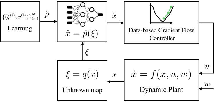
To produce estimates of the system state x^=p(ξ)^𝑥𝑝𝜉\hat{x}=p(\xi), we assume that a set of training points {(ξ(i),x(i))}i=1Nsuperscriptsubscriptsuperscript𝜉𝑖superscript𝑥𝑖𝑖1𝑁\{(\xi^{(i)},x^{(i)})\}_{i=1}^{N} is utilized to train a neural network via empirical risk minimization. More precisely, in the remainder, we will study two types of neural networks that can be used for this purpose: (i) feedforward neural networks, and (ii) residual neural networks222We refer the reader to the representative papers [25, 28] for an overview of feedforward and residual networks. Briefly, a neural network consists of inputs, various hidden layers, activation functions, and output layers, and can be trained for, e.g., functional estimation and classification. When the layers are sequential and the architecture is described by a directed acyclic graph, the underlying network is called feedforward; when some of these layers are bypassed, then the underlying network is called residual.. We thus propose to train a neural network to produce a map x^=p^(ξ)^𝑥^𝑝𝜉\hat{x}=\hat{p}(\xi) that yields estimates of the system state given nonlinear and high-dimensional observations ξ𝜉\xi. Accordingly, we modify the controller (6) to operate with estimates of the system state x^^𝑥\hat{x} produced by the neural network. The proposed framework is described in Algorithm 1 and illustrated in Figure 2.

Algorithm 1 Optimization with NN State Perception

# Training

Given: training set {(x(i),ξ(i))}i=1Nsuperscriptsubscriptsuperscript𝑥𝑖superscript𝜉𝑖𝑖1𝑁\{(x^{(i)},\xi^{(i)})\}_{i=1}^{N}

Obtain: p^NNlearning({(x(i),ξ(i))}i=1N)\hat{p}\leftarrow\operatorname{NN-learning}(\{(x^{(i)},\xi^{(i))}\}_{i=1}^{N})

# Gradient-based Feedback Control

Given: set 𝒰𝒰\mathcal{U}, funct.s ϕ,ψ,H(u)italic-ϕ𝜓𝐻𝑢\nabla\phi,\nabla\psi,H(u), neural net p^^𝑝\hat{p}, gain η𝜂\eta

Initial conditions: x(t0)𝒳0𝑥subscript𝑡0subscript𝒳0x(t_{0})\in\mathcal{X}_{0}, u(t0)𝒰𝑢subscript𝑡0𝒰u(t_{0})\in\mathcal{U}

For tt0𝑡subscript𝑡0t\geq t_{0}:

x˙˙𝑥\displaystyle\dot{x} =f(x,u,wt)absent𝑓𝑥𝑢subscript𝑤𝑡\displaystyle=f(x,u,w_{t}) (12a)
ξ𝜉\displaystyle\xi =q(x)absent𝑞𝑥\displaystyle=q(x) (12b)
u˙˙𝑢\displaystyle\dot{u} =Π𝒞{uη(ϕ(u)+H(u)ψ(p^(ξ)))}uabsentsubscriptΠ𝒞𝑢𝜂italic-ϕ𝑢𝐻superscript𝑢top𝜓^𝑝𝜉𝑢\displaystyle=\Pi_{\mathcal{C}}\left\{u-\eta\left(\nabla\phi(u)+H(u)^{\top}\nabla\psi(\hat{p}(\xi))\right)\right\}-u (12c)
Refer to caption
Figure 2: Schematics of the control framework proposed in Algorithm 1. In this setting, the state x𝑥x of the system is not measurable directly, instead, only high-dimensional estimations (e.g., camera images) ξ=q(x)𝜉𝑞𝑥\xi=q(x) are available. A deep neural network is then used to compute state estimates x^=p^(ξ)^𝑥^𝑝𝜉\hat{x}=\hat{p}(\xi), which are used to feed a gradient-based feedback controller).

In the training phase of Algorithm 1, the map NNlearning()NNlearning\operatorname{NN-learning}(\cdot) denotes a generic training procedure for the neural network via empirical risk minimization. The output of the training phase is the neural network mapping p^()^𝑝\hat{p}(\cdot). In the feedback control phase, the map p^()^𝑝\hat{p}(\cdot) is then used to produce estimates of the state of the dynamical system x^=p^(ξ)^𝑥^𝑝𝜉\hat{x}=\hat{p}(\xi) in order to evaluate the gradient functions. Notice that, relative to the nominal controller (6), (12c) leverages a gradient that is evaluated at an approximate point x^^𝑥\hat{x}, and thus fits the more general model (7b).

4.2 Analysis of Algorithm 1

In what follows, we analyze the tracking properties of Algorithm 1. To this end, we introduce the following.

Assumption 6 (Generative and Perception Maps)

The generative map xq(x)=ξmaps-to𝑥𝑞𝑥𝜉x\mapsto q(x)=\xi is such that, for any compact set 𝒳𝒳rsuperscript𝒳subscript𝒳𝑟\mathcal{X}^{\prime}\subseteq\mathcal{X}_{r}, the image q(𝒳)𝑞superscript𝒳q(\mathcal{X}^{\prime}) is compact. Moreover, there exists a continuous p:nξn:𝑝superscriptsubscript𝑛𝜉superscript𝑛p:\mathbb{R}^{n_{\xi}}\to\mathbb{R}^{n} such that p(ξ)=x𝑝𝜉𝑥p(\xi)=x for any x𝒳r𝑥subscript𝒳𝑟x\in\mathcal{X}_{r}, where ξ=q(x)𝜉𝑞𝑥\xi=q(x). \square

Remark 4.8 (Relationship with System Observability).

We note that a standard approach in the literature for the state observer design problem is to leverage the concept of \ell-observability, where the state is estimated based on +11\ell+1 samples of ξ𝜉\xi and \ell samples of the inputs u,w𝑢𝑤u,w [3]. However, we note that in our setup we do not have access to measurements of the exogenous input wtsubscript𝑤𝑡w_{t}; therefore, we rely on an approach similar to [1, 2] where x𝑥x is estimated from the observation ξ𝜉\xi. \square

To guarantee that network training is well-posed, we assume that the N𝑁N training points {x(i)}i=1Nsuperscriptsubscriptsuperscript𝑥𝑖𝑖1𝑁\{x^{(i)}\}_{i=1}^{N} for the state are drawn from a compact set 𝒳train:=𝒳eq+n[rtrain]assignsubscript𝒳trainsubscript𝒳eqsubscript𝑛delimited-[]subscript𝑟train\mathcal{X}_{\textrm{train}}:={\mathcal{X}}_{\textup{eq}}+\mathcal{B}_{n}[r_{\textrm{train}}], where rtrainsubscript𝑟trainr_{\textrm{train}} is such that r0rtrain<rsubscript𝑟0subscript𝑟train𝑟r_{0}\leq r_{\textrm{train}}<r. Moreover, we let 𝒬train:=q(𝒳train)assignsubscript𝒬train𝑞subscript𝒳train\mathcal{Q}_{\textrm{train}}:=q(\mathcal{X}_{\textrm{train}}) denote the perception set associated with the training set 𝒳trainsubscript𝒳train\mathcal{X}_{\textrm{train}}, and we denote by 𝒬train,s:={ξ(i)=q(x(i)),i=1,,N}𝒬trainassignsubscript𝒬train𝑠formulae-sequencesuperscript𝜉𝑖𝑞superscript𝑥𝑖𝑖1𝑁subscript𝒬train\mathcal{Q}_{\textrm{train},s}:=\{\xi^{(i)}=q(x^{(i)}),i=1,\ldots,N\}\subset\mathcal{Q}_{\textrm{train}} the set of available perception samples. Notice that the set 𝒬trainsubscript𝒬train\mathcal{Q}_{\textrm{train}} is compact by Assumption 6. Compactess of 𝒬trainsubscript𝒬train\mathcal{Q}_{\textrm{train}} will allow us to build on the results of [25] and [3, 27] to bound the perception error p(ξ)p^(ξ)norm𝑝𝜉^𝑝𝜉\|p(\xi)-\hat{p}(\xi)\| on the compact set 𝒬trainsubscript𝒬train\mathcal{Q}_{\textrm{train}}. With this background, we let supξ𝒬train,sp(ξ)p^(ξ)subscriptsupremum𝜉subscript𝒬train,ssubscriptnorm𝑝𝜉^𝑝𝜉\sup_{\xi\in\mathcal{Q}_{\textrm{train,s}}}\|p(\xi)-\hat{p}(\xi)\|_{\infty} denote the supremum norm of the approximation error over 𝒬train,ssubscript𝒬train,s\mathcal{Q}_{\textrm{train,s}}.

Remark 4.9 (Properties of the Training Set).

Notice that the set of training data 𝒳trainsubscript𝒳train\mathcal{X}_{\textrm{train}} is assumed to contain the set of initial conditions 𝒳0subscript𝒳0\mathcal{X}_{0}. This allows us to guarantee that the neural network can be trained over the domain of definition of the Lyapunov function W𝑊W in Lemma 1 (see Figure 1 for an illustration). If, by contrast, the set 𝒳trainsubscript𝒳train\mathcal{X}_{\textrm{train}} were contained in 𝒳0subscript𝒳0\mathcal{X}_{0}, then the set of initial of (12) must be modified so that the trajectories do not leave the set 𝒳trainsubscript𝒳train\mathcal{X}_{\textrm{train}}. \square

We begin by characterizing the performance of (12) when residual networks are utilized to reconstruct the system state. For simplicity of exposition, we outline the main result for the case where n=nξ𝑛subscript𝑛𝜉n=n_{\xi}, and we then discuss how to consider the case n<nξ𝑛subscript𝑛𝜉n<n_{\xi} in Remark 4.12.

Proposition 4.10.

(Transient Performance of Algorithm 1 with Residual Neural Network) Consider the closed-loop system (12), let Assumptions 1-6 be satisfied, and assume n=nξ𝑛subscript𝑛𝜉n=n_{\xi}. Assume that the training set 𝒬train,ssubscript𝒬train𝑠\mathcal{Q}_{\textrm{train},s} is a ϱitalic-ϱ\varrho-cover of 𝒬trainsubscript𝒬train\mathcal{Q}_{\textrm{train}} with respect to the partial order precedes-or-equals\preceq, for some ϱ>0italic-ϱ0\varrho>0. Let presNet:nξRnξ:subscript𝑝resNetsuperscriptsubscript𝑛𝜉superscript𝑅subscript𝑛𝜉p_{\textrm{resNet}}:\mathbb{R}^{n_{\xi}}\to R^{n_{\xi}} describe a residual network, and assume that it can be decomposed as presNet=m+Asubscript𝑝resNet𝑚𝐴p_{\textrm{resNet}}=m+A, where m:nξnξ:𝑚superscriptsubscript𝑛𝜉superscriptsubscript𝑛𝜉m:\mathbb{R}^{n_{\xi}}\to\mathbb{R}^{n_{\xi}} is monotone and A:nξnξ:𝐴superscriptsubscript𝑛𝜉superscriptsubscript𝑛𝜉A:\mathbb{R}^{n_{\xi}}\to\mathbb{R}^{n_{\xi}} is a linear function. If Algorithm 1 is implemented with p^=presNet^𝑝subscript𝑝resNet\hat{p}=p_{\textrm{resNet}} and η(0,η)𝜂0superscript𝜂\eta\in(0,\eta^{*}), then the error z(t)=(xxt,uut)𝑧𝑡𝑥subscriptsuperscript𝑥𝑡𝑢subscriptsuperscript𝑢𝑡z(t)=(x-x^{*}_{t},u-u^{*}_{t}) of (12) satisfies (11) with κ1,κ2,κ3subscript𝜅1subscript𝜅2subscript𝜅3\kappa_{1},\kappa_{2},\kappa_{3} as in Theorem 3.7, γ=0𝛾0\gamma=0, and

δ𝛿\displaystyle\delta =huxnξ(3supξ𝒬train,sp(ξ)presNet(ξ)\displaystyle=\ell_{h_{u}}\ell_{x}\sqrt{n_{\xi}}\Big{(}3\sup_{\xi\in\mathcal{Q}_{\textrm{train},s}}\|p(\xi)-p_{\textrm{resNet}}(\xi)\|_{\infty}
+2ωp(ϱ)+2Aϱ)\displaystyle\hskip 110.96556pt+2\,\omega_{p}(\varrho)+2\|A\|_{\infty}\varrho\Big{)} (13)

where ωpsubscript𝜔𝑝\omega_{p} is a modulus of continuity of p𝑝p on 𝒬trainsubscript𝒬train\mathcal{Q}_{\textrm{train}}. \square

Proof 4.11.

Start by noticing that (12c) can be written in the generic form (7b) with the error e(x,u)𝑒𝑥𝑢e(x,u) given by e(u,x)=H(u)ψ(x)H(u)ψ(x^)=H(u)ψ(p(ξ))H(u)ψ(p^(ξ))𝑒𝑢𝑥𝐻superscript𝑢top𝜓𝑥𝐻superscript𝑢top𝜓^𝑥𝐻superscript𝑢top𝜓𝑝𝜉𝐻superscript𝑢top𝜓^𝑝𝜉e(u,x)=H(u)^{\top}\nabla\psi(x)-H(u)^{\top}\nabla\psi(\hat{x})=H(u)^{\top}\nabla\psi(p(\xi))-H(u)^{\top}\nabla\psi(\hat{p}(\xi)), by simply adding and subtracting the true gradient H(u)ψ(x)𝐻superscript𝑢top𝜓𝑥H(u)^{\top}\nabla\psi(x) in (12c). A uniform bound on the norm of e(u,x)𝑒𝑢𝑥e(u,x) over the compact set 𝒬trainsubscript𝒬train\mathcal{Q}_{\textrm{train}} is given by:

e(u,x)norm𝑒𝑢𝑥\displaystyle\|e(u,x)\| hu[ψ(p(ξ))ψ(p^(ξ))]absentsubscriptsubscript𝑢delimited-[]𝜓𝑝𝜉𝜓^𝑝𝜉\displaystyle\leq\ell_{h_{u}}\big{[}\nabla\psi(p(\xi))-\nabla\psi(\hat{p}(\xi))\big{]}
huxp(ξ)presNet(ξ)absentsubscriptsubscript𝑢subscript𝑥norm𝑝𝜉subscript𝑝resNet𝜉\displaystyle\leq\ell_{h_{u}}\ell_{x}\|p(\xi)-p_{\textrm{resNet}}(\xi)\|
huxsupξ𝒬trainp(ξ)presNet(ξ),absentsubscriptsubscript𝑢subscript𝑥subscriptsupremum𝜉subscript𝒬trainnorm𝑝𝜉subscript𝑝resNet𝜉\displaystyle\leq\ell_{h_{u}}\ell_{x}\sup_{\xi\in\mathcal{Q}_{\textrm{train}}}\|p(\xi)-p_{\textrm{resNet}}(\xi)\|\,, (14)

where we have used Assumption 1 and the fact that the norm of the Jacobian of hh is bounded over the compact set 𝒰𝒰\mathcal{U}. Next, notice first that p(ξ)p^(ξ)nξp(ξ)presNet(ξ)norm𝑝𝜉^𝑝𝜉subscript𝑛𝜉subscriptnorm𝑝𝜉subscript𝑝resNet𝜉\|p(\xi)-\hat{p}(\xi)\|\leq\sqrt{n_{\xi}}\|p(\xi)-p_{\textrm{resNet}}(\xi)\|_{\infty}. Since 𝒬train,ssubscript𝒬train𝑠\mathcal{Q}_{\textrm{train},s} is a ϱitalic-ϱ\varrho-cover of 𝒬dsubscript𝒬𝑑\mathcal{Q}_{d} with respect to the partial order precedes-or-equals\preceq, for some ϱ>0italic-ϱ0\varrho>0, and presNet=m+Asubscript𝑝resNet𝑚𝐴p_{\textrm{resNet}}=m+A, the infimum norm of the estimation error can be upper bounded as supξ𝒬trainp(ξ)presNet(ξ)3supξ𝒬train,sp(ξ)presNet(ξ)+2ωp(ϱ)+2Apsubscriptsupremum𝜉subscript𝒬trainsubscriptnorm𝑝𝜉subscript𝑝resNet𝜉3subscriptsupremum𝜉subscript𝒬train𝑠subscriptnorm𝑝𝜉subscript𝑝resNet𝜉2subscript𝜔𝑝italic-ϱ2subscriptnormsubscript𝐴𝑝\sup_{\xi\in\mathcal{Q}_{\textrm{train}}}\|p(\xi)-p_{\textrm{resNet}}(\xi)\|_{\infty}\leq 3\sup_{\xi\in\mathcal{Q}_{\textrm{train},s}}\|p(\xi)-p_{\textrm{resNet}}(\xi)\|_{\infty}+2\,\omega_{p}(\varrho)+2\|A_{p}\|_{\infty} as shown in [28, Theorem 7]. The result then follows from Theorem 3.7 by setting γ=0𝛾0\gamma=0 and δ𝛿\delta as in (13).

Proposition 4.10 shows that the control method in Algorithm 1 guarantees convergence to the optimizer of (4), up to an error that depends only on the uniform approximation error of the adopted neural network. Notice that supξ𝒬train,sp(ξ)presNet(ξ)subscriptsupremum𝜉subscript𝒬train𝑠subscriptnorm𝑝𝜉subscript𝑝resNet𝜉\sup_{\xi\in\mathcal{Q}_{\textrm{train},s}}\|p(\xi)-p_{\textrm{resNet}}(\xi)\|_{\infty} is a constant that denotes the worse-case approximation error of the training data over the compact set 𝒬train,ssubscript𝒬train𝑠\mathcal{Q}_{\textrm{train},s}. More precisely, the result characterizes the role of the approximation errors due to the use of a neural network in the transient and asymptotic performance of the interconnected system (12).

Remark 4.12 (Perception in High-Dimensional Spaces).

When nξ>nsubscript𝑛𝜉𝑛n_{\xi}>n, one can consider training a neural network to approximate a lifted map p~:nξnξ:~𝑝superscriptsubscript𝑛𝜉superscriptsubscript𝑛𝜉\tilde{p}:\mathbb{R}^{n_{\xi}}\to\mathbb{R}^{n_{\xi}} defined as p~=ιp~𝑝𝜄𝑝\tilde{p}=\iota\circ p, where ι:nnξ:𝜄superscript𝑛superscriptsubscript𝑛𝜉\iota:\mathbb{R}^{n}\to\mathbb{R}^{n_{\xi}} is the injection: ι(x)=(x1,,xn,0,,0)𝜄𝑥subscript𝑥1subscript𝑥𝑛00\iota(x)=(x_{1},\ldots,x_{n},0,\ldots,0) for any xn𝑥superscript𝑛x\in\mathbb{R}^{n}. From Assumption 6, it follows that p~()~𝑝\tilde{p}(\cdot) is such that p~(ξ)=(x,0qn)~𝑝𝜉𝑥subscript0𝑞𝑛\tilde{p}(\xi)=(x,0_{q-n}) for any x𝒳r𝑥subscript𝒳𝑟x\in\mathcal{X}_{r}, with ξ𝜉\xi an observation generated by the map q()𝑞q(\cdot).

In this case, we use the training set {(x(i),0qn),ξ(i)}i=1Nsuperscriptsubscriptsuperscript𝑥𝑖subscript0𝑞𝑛superscript𝜉𝑖𝑖1𝑁\{(x^{(i)},0_{q-n}),\xi^{(i)}\}_{i=1}^{N} to train the neural network implementing a map presNet:nξnξ:subscript𝑝resNetsuperscriptsubscript𝑛𝜉superscriptsubscript𝑛𝜉p_{\textrm{resNet}}:\mathbb{R}^{n_{\xi}}\to\mathbb{R}^{n_{\xi}} [3]. Subsequently, the perception map p^^𝑝\hat{p} that will be used in (12c) is given by p^=πpresNet^𝑝𝜋subscript𝑝resNet\hat{p}=\pi\circ p_{\textrm{resNet}}, where π:nξn:𝜋superscriptsubscript𝑛𝜉superscript𝑛\pi:\mathbb{R}^{n_{\xi}}\to\mathbb{R}^{n} is a projection map that returns the first n𝑛n entries of its argument, namely, π(y)=(y1,,yn)𝜋𝑦subscript𝑦1subscript𝑦𝑛\pi(y)=(y_{1},\ldots,y_{n}), for any yq𝑦superscript𝑞y\in\mathbb{R}^{q}. Summarizing, the training step NNlearning()NNlearning\operatorname{NN-learning}(\cdot) in Algorithm 1 in this case involves the training of the map presNetsubscript𝑝resNetp_{\textrm{resNet}}, followed by the projection x^=p^(ξ)=π(p claim(ξ))^𝑥^𝑝𝜉𝜋subscript𝑝 claim𝜉\hat{x}=\hat{p}(\xi)=\pi(p_{\textrm{ claim}}(\xi)). Finally, we notice that in this case the claim in Proposition 4.11 holds unchanged by replacing p(ξ)𝑝𝜉p(\xi) with p~(ξ)~𝑝𝜉\tilde{p}(\xi). This follows by noting that p(ξ)p^(ξ)nξp(ξ)presNet(ξ)norm𝑝𝜉^𝑝𝜉subscript𝑛𝜉subscriptnorm𝑝𝜉subscript𝑝resNet𝜉\|p(\xi)-\hat{p}(\xi)\|\leq\sqrt{n_{\xi}}\|p(\xi)-p_{\textrm{resNet}}(\xi)\|_{\infty}. \square

Remark 4.13 (Density of Training Set).

Proposition 4.10 requires the training set 𝒬train,ssubscript𝒬train𝑠\mathcal{Q}_{\textrm{train},s} is a ϱitalic-ϱ\varrho-cover of 𝒬trainsubscript𝒬train\mathcal{Q}_{\textrm{train}}, with respect to the partial order precedes-or-equals\preceq. As pointed out in [3], verifying this condition often involves computing the relative position of the training points and the points in the set 𝒬trainsubscript𝒬train\mathcal{Q}_{\textrm{train}}. When this is not possible, [3, Lemma 2] shows that there exists a relationship between ϱitalic-ϱ\varrho-covering of the set 𝒬trainsubscript𝒬train\mathcal{Q}_{\textrm{train}} with respect to precedes-or-equals\preceq and the density of the training points. In particular, the authors show that if the set of training points is a ϱsuperscriptitalic-ϱ\varrho^{\prime}-cover of 𝒬trainsubscript𝒬train\mathcal{Q}_{\textrm{train}}, then it is also a ϱitalic-ϱ\varrho-covering for a set the set 𝒬trainsuperscriptsubscript𝒬train\mathcal{Q}_{\textrm{train}}^{\prime}, 𝒬train𝒬trainsubscript𝒬trainsuperscriptsubscript𝒬train\mathcal{Q}_{\textrm{train}}\subset\mathcal{Q}_{\textrm{train}}^{\prime}, with respect to precedes-or-equals\preceq, for some ϱ>ϱitalic-ϱsuperscriptitalic-ϱ\varrho>\varrho^{\prime}; see [3, Lemma 2]. \square

In the remainder of this section, we focus on characterizing the performance of (12) when a feedforward network is utilized to reconstruct the system state. More precisely, we consider cases where the training set {ξ(i),x(i)}i=1Nsuperscriptsubscriptsuperscript𝜉𝑖superscript𝑥𝑖𝑖1𝑁\{\xi^{(i)},x^{(i)}\}_{i=1}^{N} is utilized to train n𝑛n multilayer feedforward networks, each of them implementing a map pfeedNet,i:nξ:subscript𝑝feedNet𝑖superscriptsubscript𝑛𝜉p_{\textrm{feedNet},i}:\mathbb{R}^{n_{\xi}}\to\mathbb{R} that estimates the i𝑖i-th component of the system state x^i=pfeedNet,i(ξ)subscript^𝑥𝑖subscript𝑝feedNet𝑖𝜉\hat{x}_{i}=p_{\textrm{feedNet},i}(\xi). In this case, we assume that Algorithm 1 is implemented with p^=pfeedNet^𝑝subscript𝑝feedNet\hat{p}=p_{\textrm{feedNet}}, where pfeedNet(ξ):=(pfeedNet,1(ξ),,pfeedNet,n(ξ))assignsubscript𝑝feedNet𝜉subscript𝑝feedNet1𝜉subscript𝑝feedNet𝑛𝜉p_{\textrm{feedNet}}(\xi):=(p_{\textrm{feedNet},1}(\xi),\ldots,p_{\textrm{feedNet},n}(\xi)) in (12). Next, we recall that feedforward neural networks are capable of approximating any measurable function on compact sets with any desired degree of accuracy (see, for instance, [25, 26] and the bounds in [56, 57]).

Proposition 4.14.

(Transient Performance of Algorithm 1 with Feedforward Neural Network) Consider the closed-loop system (12) and let Assumptions 1-6 be satisfied. Suppose that p^(ξ)=(pfeedNet,1(ξ),,pfeedNet,n(ξ))^𝑝𝜉subscript𝑝feedNet1𝜉subscript𝑝feedNet𝑛𝜉\hat{p}(\xi)=(p_{\textrm{feedNet},1}(\xi),\ldots,p_{\textrm{feedNet},n}(\xi)), with pfeedNet,isubscript𝑝feedNet𝑖p_{\textrm{feedNet},i} approximating the map pi(ξ)subscript𝑝𝑖𝜉p_{i}(\xi). Then, if η(0,η)𝜂0superscript𝜂\eta\in(0,\eta^{*}), the error z(t)=(xxt,uut)𝑧𝑡𝑥subscriptsuperscript𝑥𝑡𝑢subscriptsuperscript𝑢𝑡z(t)=(x-x^{*}_{t},u-u^{*}_{t}) of (12) satisfies (11) with γ=0𝛾0\gamma=0,

δ𝛿\displaystyle\delta =huxnsupξ𝒬trainp(ξ)pfeedNet(ξ),absentsubscriptsubscript𝑢subscript𝑥𝑛subscriptsupremum𝜉subscript𝒬trainsubscriptnorm𝑝𝜉subscript𝑝feedNet𝜉\displaystyle=\ell_{h_{u}}\ell_{x}\sqrt{n}\sup_{\xi\in\mathcal{Q}_{\textrm{train}}}\|p(\xi)-p_{\textrm{feedNet}}(\xi)\|_{\infty}\,, (15)

and κ1,κ2,κ3subscript𝜅1subscript𝜅2subscript𝜅3\kappa_{1},\kappa_{2},\kappa_{3} as in Theorem 3.7. \square

The proof follows similar steps as in Proposition 4.10, and it is omitted. Proposition 4.14 shows that the control method in Algorithm 1 guarantees convergence to the optimizer of (4), up to an error that depends only on the uniform approximation error supξ𝒬trainp(ξ)pfeedNet(ξ)subscriptsupremum𝜉subscript𝒬trainsubscriptnorm𝑝𝜉subscript𝑝feedNet𝜉\sup_{\xi\in\mathcal{Q}_{\textrm{train}}}\|p(\xi)-p_{\textrm{feedNet}}(\xi)\|_{\infty} (computed over the entire training set 𝒬trainsubscript𝒬train\mathcal{Q}_{\textrm{train}}). Notice that, with respect to Proposition 4.10, the adoption of a feedforward network allows us to provide tighter guarantees in terms of the entire set 𝒬trainsubscript𝒬train\mathcal{Q}_{\textrm{train}} (as opposed to the set of available samples 𝒬train,ssubscript𝒬train𝑠\mathcal{Q}_{\textrm{train},s}). We conclude by noting that the bound (15) can be further customized for specific error bounds, given the architecture of the feedforward network [56, 57].

Remark 4.15 (Noisy generative and perception maps).

Assumption 6 is borrowed from [2] and it holds when, for example, q𝑞q is injective. Although the model in Assumption 6 is used for simplicity, the subsequent analysis of our perception-based controllers can be readily extended to the case where: (i) the perception map imperfectly estimates the state; that is, one has that p(ξ)=x+ν𝑝𝜉𝑥𝜈p(\xi)=x+\nu, with ξ=q(x)𝜉𝑞𝑥\xi=q(x), and where νn𝜈superscript𝑛\nu\in\mathbb{R}^{n} is a bounded error [1]. (ii) When unknown externalities enter the generative map. One way to collectively account for both externalities entering q𝑞q and for approximate perception map is to use the noisy model p(q(x))=x+ν𝑝𝑞𝑥𝑥superscript𝜈p(q(x))=x+\nu^{\prime}, with νnsuperscript𝜈superscript𝑛\nu^{\prime}\in\mathbb{R}^{n} a given error (bounded in norm). The results presented in this section can be readily modified to account for this additional error by adding a term proportional to the norm of νsuperscript𝜈\nu^{\prime} in the parameter δ𝛿\delta.

5 Optimization with Cost-Function Perception

In this section, we propose an algorithm to address Problem 2.4, and we tailor the conclusions drawn in Theorem 3.7 to characterize the performance of the proposed algorithm.

5.1 Algorithm Description

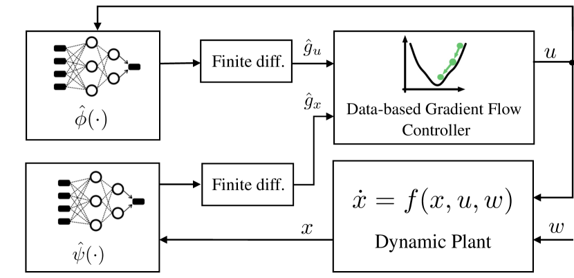
To determine estimates of the gradient functions ϕ(u),ψ(x)italic-ϕ𝑢𝜓𝑥\nabla\phi(u),\nabla\psi(x), we assume the availability of functional evaluations {(u(i),ϕ(u(i)))}i=1Nsuperscriptsubscriptsuperscript𝑢𝑖italic-ϕsuperscript𝑢𝑖𝑖1𝑁\{(u^{(i)},\phi(u^{(i)}))\}_{i=1}^{N} and {(x(i),ψ(x(i)))}i=1Msuperscriptsubscriptsuperscript𝑥𝑖𝜓superscript𝑥𝑖𝑖1𝑀\{(x^{(i)},\psi(x^{(i)}))\}_{i=1}^{M}, with u(i)𝒞superscript𝑢𝑖𝒞u^{(i)}\in\mathcal{C} and x(i)𝒳trainsuperscript𝑥𝑖subscript𝒳trainx^{(i)}\in\mathcal{X}_{\textrm{train}}. We then consider the training of two neural networks that approximate the functions uϕ(u)maps-to𝑢italic-ϕ𝑢u\mapsto\phi(u) and xψ(x)maps-to𝑥𝜓𝑥x\mapsto\psi(x), respectively, to determine ϕ^(u)^italic-ϕ𝑢\hat{\phi}(u), ψ^(x)^𝜓𝑥\hat{\psi}(x). Accordingly, we modify the controller (6) to operate with estimates of the system state x^^𝑥\hat{x} produced by the neural network. The proposed framework is described in Algorithm 2 and illustrated in Figure 3.

Algorithm 2 Optimization with NN Cost Perception

# Training

Given: {u(i),ϕ(u(i))}i=1Nsuperscriptsubscriptsuperscript𝑢𝑖italic-ϕsuperscript𝑢𝑖𝑖1𝑁\{u^{(i)},\phi(u^{(i)})\}_{i=1}^{N}, {x(i),ψ(x(i))}i=1Msuperscriptsubscriptsuperscript𝑥𝑖𝜓superscript𝑥𝑖𝑖1𝑀\{x^{(i)},\psi(x^{(i)})\}_{i=1}^{M}

Obtain:

ϕ^^italic-ϕ\displaystyle\hat{\phi} NNlearning({(u(i),ϕ(u(i)))}i=1N)absentNNlearningsuperscriptsubscriptsuperscript𝑢𝑖italic-ϕsuperscript𝑢𝑖𝑖1𝑁\displaystyle\leftarrow\operatorname{NN-learning}(\{(u^{(i)},\phi(u^{(i)}))\}_{i=1}^{N})
ψ^^𝜓\displaystyle\hat{\psi} NNlearning({(x(i),ψ(x(i)))}i=1M)absentNNlearningsuperscriptsubscriptsuperscript𝑥𝑖𝜓superscript𝑥𝑖𝑖1𝑀\displaystyle\leftarrow\operatorname{NN-learning}(\{(x^{(i)},\psi(x^{(i)}))\}_{i=1}^{M})

# Gradient-based Feedback Control

Given: x(t0)𝒟0𝑥subscript𝑡0subscript𝒟0x(t_{0})\in\mathcal{D}_{0}, u(t0)𝒞𝑢subscript𝑡0𝒞u(t_{0})\in\mathcal{C}, NN maps ϕ^,ψ^^italic-ϕ^𝜓\hat{\phi},\hat{\psi}.

For tt0𝑡subscript𝑡0t\geq t_{0}:

x˙˙𝑥\displaystyle\dot{x} =f(x,u,wt)absent𝑓𝑥𝑢subscript𝑤𝑡\displaystyle=f(x,u,w_{t}) (16a)
g^u(u)subscript^𝑔𝑢𝑢\displaystyle\hat{g}_{u}(u) =i=1nu12ε(ϕ^(u+εbi)ϕ^(uεbi))bi,absentsuperscriptsubscript𝑖1subscript𝑛𝑢12𝜀^italic-ϕ𝑢𝜀subscript𝑏𝑖^italic-ϕ𝑢𝜀subscript𝑏𝑖subscript𝑏𝑖\displaystyle=\sum_{i=1}^{n_{u}}\frac{1}{2\varepsilon}\left(\hat{\phi}(u+\varepsilon b_{i})-\hat{\phi}(u-\varepsilon b_{i})\right)b_{i}, (16b)
g^x(x)subscript^𝑔𝑥𝑥\displaystyle\hat{g}_{x}(x) =i=1n12ε(ψ^(x+εdi)ψ^(xεdi))di,absentsuperscriptsubscript𝑖1𝑛12𝜀^𝜓𝑥𝜀subscript𝑑𝑖^𝜓𝑥𝜀subscript𝑑𝑖subscript𝑑𝑖\displaystyle=\sum_{i=1}^{n}\frac{1}{2\varepsilon}\left(\hat{\psi}(x+\varepsilon d_{i})-\hat{\psi}(x-\varepsilon d_{i})\right)d_{i}, (16c)
u˙˙𝑢\displaystyle\dot{u} =Π𝒞{uη(g^u(u)+H(u)g^x(x))}uabsentsubscriptΠ𝒞𝑢𝜂subscript^𝑔𝑢𝑢𝐻superscript𝑢topsubscript^𝑔𝑥𝑥𝑢\displaystyle=\Pi_{\mathcal{C}}\left\{u-\eta\left(\hat{g}_{u}(u)+H(u)^{\top}\hat{g}_{x}(x)\right)\right\}-u (16d)
Refer to caption
Figure 3: Schematics of the control framework proposed in Algorithm 2. A gradient-based controller is utilized to control the system to the optimizer of an unknown cost function. The underlying cost function is estimated from data samples through a residual neural network.

In Algorithm 2, the gradients of the costs are obtained via centered difference, applied to the estimated maps ϕ^^italic-ϕ\hat{\phi} and ψ^^𝜓\hat{\psi}, where ε>0𝜀0\varepsilon>0, bisubscript𝑏𝑖b_{i} denotes the i𝑖i-th canonical vector of nusuperscriptsubscript𝑛𝑢\mathbb{R}^{n_{u}}, and disubscript𝑑𝑖d_{i} is the the i𝑖i-th canonical vector of nsuperscript𝑛\mathbb{R}^{n}. The computation of the approximate gradient g^usubscript^𝑔𝑢\hat{g}_{u} (respectively, g^xsubscript^𝑔𝑥\hat{g}_{x}) thus requires 2nu2subscript𝑛𝑢2n_{u} functional evaluations (respectively, 2n2𝑛2n) of the neural network map ϕ^^italic-ϕ\hat{\phi} (respectively, ψ^^𝜓\hat{\psi}). The gradient estimates g^usubscript^𝑔𝑢\hat{g}_{u} and g^xsubscript^𝑔𝑥\hat{g}_{x} are then utilized in the gradient-based feedback controller (16d).

5.2 Analysis of Algorithm 2

We begin by characterizing the performance of (16) when feedforward networks are utilized to estimate the costs.

Proposition 5.16.

(Transient Performance of Algorithm 2 with Feedforward Neural Network) Suppose that feedforward network maps ϕ^feedNetsubscript^italic-ϕfeedNet\hat{\phi}_{\textrm{feedNet}} and ψ^feedNetsubscript^𝜓feedNet\hat{\psi}_{\textrm{feedNet}} approximate the costs ϕitalic-ϕ\phi and ϕitalic-ϕ\phi over the compact sets 𝒳trainsubscript𝒳train\mathcal{X}_{\textrm{train}} and 𝒞train:=𝒞+[ε]assignsubscript𝒞train𝒞delimited-[]𝜀\mathcal{C}_{\textrm{train}}:=\mathcal{C}+\mathcal{B}[\varepsilon], respectively. Consider the interconnected system (16), with ϕ^=ϕ^feedNet^italic-ϕsubscript^italic-ϕfeedNet\hat{\phi}=\hat{\phi}_{\textrm{feedNet}} and ψ^=ψ^feedNet^𝜓subscript^𝜓feedNet\hat{\psi}=\hat{\psi}_{\textrm{feedNet}}, and let Assumptions 1-5 be satisfied. If η(0,η)𝜂0superscript𝜂\eta\in(0,\eta^{*}), then error z(t)=(xxt,uut)𝑧𝑡𝑥subscriptsuperscript𝑥𝑡𝑢subscriptsuperscript𝑢𝑡z(t)=(x-x^{*}_{t},u-u^{*}_{t}) satisfies (11) with κ1,κ2,κ3subscript𝜅1subscript𝜅2subscript𝜅3\kappa_{1},\kappa_{2},\kappa_{3} as in Theorem 3.7, γ=0𝛾0\gamma=0, and

δ𝛿\displaystyle\delta =eu,fd+nuε1supu𝒞train|ϕ(u)ϕ^feedNet(u)|absentsubscript𝑒𝑢fdsubscript𝑛𝑢superscript𝜀1subscriptsupremum𝑢subscript𝒞trainitalic-ϕ𝑢subscript^italic-ϕfeedNet𝑢\displaystyle=e_{u,\textrm{fd}}+n_{u}\varepsilon^{-1}\sup_{u\in\mathcal{C}_{\textrm{train}}}|\phi(u)-\hat{\phi}_{\textrm{feedNet}}(u)|
+huex,fd+nε1husupu𝒳train|ψ(x)ψ^feedNet(x)|,subscriptsubscript𝑢subscript𝑒𝑥fd𝑛superscript𝜀1subscriptsubscript𝑢subscriptsupremum𝑢subscript𝒳train𝜓𝑥subscript^𝜓feedNet𝑥\displaystyle~{}~{}+\ell_{h_{u}}e_{x,\textrm{fd}}+n\varepsilon^{-1}\ell_{h_{u}}\sup_{u\in\mathcal{X}_{\textrm{train}}}|\psi(x)-\hat{\psi}_{\textrm{feedNet}}(x)|, (17)

where ex,fdsubscript𝑒𝑥fde_{x,\textrm{fd}} and ex,fdsubscript𝑒𝑥fde_{x,\textrm{fd}} are bounds on the centered difference approximation error for the functions ϕitalic-ϕ\phi and ψ𝜓\psi, respectively; namely, eu,fd=supu𝒞trainϕ(u)i=1nu12ε(ϕ(u+εbi)ϕ(uεbi))bisubscript𝑒𝑢fdsubscriptsupremum𝑢subscript𝒞trainnormitalic-ϕ𝑢superscriptsubscript𝑖1subscript𝑛𝑢12𝜀italic-ϕ𝑢𝜀subscript𝑏𝑖italic-ϕ𝑢𝜀subscript𝑏𝑖subscript𝑏𝑖e_{u,\textrm{fd}}=\sup_{u\in\mathcal{C}_{\textrm{train}}}\|\nabla\phi(u)-\sum_{i=1}^{n_{u}}\frac{1}{2\varepsilon}\left(\phi(u+\varepsilon b_{i})-\phi(u-\varepsilon b_{i})\right)b_{i}\| and ex,fd=supx𝒳trainψ(x)i=1n12ε(ψ(x+εdi)ψ(xεdi))disubscript𝑒𝑥fdsubscriptsupremum𝑥subscript𝒳trainnorm𝜓𝑥superscriptsubscript𝑖1𝑛12𝜀𝜓𝑥𝜀subscript𝑑𝑖𝜓𝑥𝜀subscript𝑑𝑖subscript𝑑𝑖e_{x,\textrm{fd}}=\sup_{x\in\mathcal{X}_{\textrm{train}}}\|\nabla\psi(x)-\sum_{i=1}^{n}\frac{1}{2\varepsilon}\left(\psi(x+\varepsilon d_{i})-\psi(x-\varepsilon d_{i})\right)d_{i}\|. \square

Proof 5.17.

We start rewriting (16d) as (7b) by setting e(x,u)=ϕ(u)g^u(u)+H(ψ(x)g^x(x))𝑒𝑥𝑢italic-ϕ𝑢subscript^𝑔𝑢𝑢superscript𝐻top𝜓𝑥subscript^𝑔𝑥𝑥e(x,u)=\nabla\phi(u)-\hat{g}_{u}(u)+H^{\top}(\nabla\psi(x)-\hat{g}_{x}(x)). Let gu(u):=i=1nu12ε(ϕ(u+εbi)ϕ(uεbi))biassignsubscript𝑔𝑢𝑢superscriptsubscript𝑖1subscript𝑛𝑢12𝜀italic-ϕ𝑢𝜀subscript𝑏𝑖italic-ϕ𝑢𝜀subscript𝑏𝑖subscript𝑏𝑖g_{u}(u):=\sum_{i=1}^{n_{u}}\frac{1}{2\varepsilon}\left(\phi(u+\varepsilon b_{i})-\phi(u-\varepsilon b_{i})\right)b_{i} and gx(x):=i=1n12ε(ψ(x+εdi)ψ(xεdi))diassignsubscript𝑔𝑥𝑥superscriptsubscript𝑖1𝑛12𝜀𝜓𝑥𝜀subscript𝑑𝑖𝜓𝑥𝜀subscript𝑑𝑖subscript𝑑𝑖g_{x}(x):=\sum_{i=1}^{n}\frac{1}{2\varepsilon}\left(\psi(x+\varepsilon d_{i})-\psi(x-\varepsilon d_{i})\right)d_{i} be the finite difference approximations of the true gradients for brevity. Adding and subtracting gu(u)subscript𝑔𝑢𝑢g_{u}(u) and gx(x)subscript𝑔𝑥𝑥g_{x}(x) using the triangle inequality, and Assumption 1, we get e(x,u)ϕ(u)gu(u)+gu(u)g^u(u)+huψ(x)gx(x)+hugx(x)g^x(x)norm𝑒𝑥𝑢normitalic-ϕ𝑢subscript𝑔𝑢𝑢normsubscript𝑔𝑢𝑢subscript^𝑔𝑢𝑢subscriptsubscript𝑢norm𝜓𝑥subscript𝑔𝑥𝑥subscriptsubscript𝑢normsubscript𝑔𝑥𝑥subscript^𝑔𝑥𝑥\|e(x,u)\|\leq\|\nabla\phi(u)-g_{u}(u)\|+\|g_{u}(u)-\hat{g}_{u}(u)\|+\ell_{h_{u}}\|\nabla\psi(x)-g_{x}(x)\|+\ell_{h_{u}}\|g_{x}(x)-\hat{g}_{x}(x)\|. The terms ϕ(u)gu(u)normitalic-ϕ𝑢subscript𝑔𝑢𝑢\|\nabla\phi(u)-g_{u}(u)\| and ψ(x)gx(x)norm𝜓𝑥subscript𝑔𝑥𝑥\|\nabla\psi(x)-g_{x}(x)\| are errors due to a finite difference approximation of the true gradients, and are bounded by eu,fdsubscript𝑒𝑢fde_{u,\textrm{fd}} and ex,fdsubscript𝑒𝑥fde_{x,\textrm{fd}}, respectively. On the other hand, gu(u)g^u(u)normsubscript𝑔𝑢𝑢subscript^𝑔𝑢𝑢\|g_{u}(u)-\hat{g}_{u}(u)\| can be bounded as:

gu(u)g^u(u)=i=1nu12ε(ϕ(u+εbi)ϕ(uεbi))bi\displaystyle\|g_{u}(u)-\hat{g}_{u}(u)\|=\Big{\|}\sum_{i=1}^{n_{u}}\frac{1}{2\varepsilon}\left(\phi(u+\varepsilon b_{i})-\phi(u-\varepsilon b_{i})\right)b_{i}
i=1nu12ε(ϕ^feedNet(u+εbi)ϕ^feedNet(uεbi))bi\displaystyle~{}~{}~{}~{}~{}-\sum_{i=1}^{n_{u}}\frac{1}{2\varepsilon}\left(\hat{\phi}_{\textrm{feedNet}}(u+\varepsilon b_{i})-\hat{\phi}_{\textrm{feedNet}}(u-\varepsilon b_{i})\right)b_{i}\Big{\|}
i=1nu12ε|ϕ(u+εbi)ϕ^feedNet(u+εbi)|biabsentsuperscriptsubscript𝑖1subscript𝑛𝑢12𝜀italic-ϕ𝑢𝜀subscript𝑏𝑖subscript^italic-ϕfeedNet𝑢𝜀subscript𝑏𝑖normsubscript𝑏𝑖\displaystyle~{}~{}\leq\sum_{i=1}^{n_{u}}\frac{1}{2\varepsilon}|\phi(u+\varepsilon b_{i})-\hat{\phi}_{\textrm{feedNet}}(u+\varepsilon b_{i})|\|b_{i}\|
+i=1nu12ε|ϕ^feedNet(uεbi)ϕ(uεbi)|bisuperscriptsubscript𝑖1subscript𝑛𝑢12𝜀subscript^italic-ϕfeedNet𝑢𝜀subscript𝑏𝑖italic-ϕ𝑢𝜀subscript𝑏𝑖normsubscript𝑏𝑖\displaystyle~{}~{}~{}~{}~{}+\sum_{i=1}^{n_{u}}\frac{1}{2\varepsilon}|\hat{\phi}_{\textrm{feedNet}}(u-\varepsilon b_{i})-\phi(u-\varepsilon b_{i})|\|b_{i}\|
nu2εsupu𝒞+[ε]|ϕ(u)ϕ^feedNet(u)|absentsubscript𝑛𝑢2𝜀subscriptsupremum𝑢𝒞delimited-[]𝜀italic-ϕ𝑢subscript^italic-ϕfeedNet𝑢\displaystyle~{}~{}\leq\frac{n_{u}}{2\varepsilon}\sup_{u\in\mathcal{C}+\mathcal{B}[\varepsilon]}|\phi(u)-\hat{\phi}_{\textrm{feedNet}}(u)| (18)

where we used the fact that bi=1normsubscript𝑏𝑖1\|b_{i}\|=1. Similar steps can be used to bound the error term gx(x)g^x(x)normsubscript𝑔𝑥𝑥subscript^𝑔𝑥𝑥\|g_{x}(x)-\hat{g}_{x}(x)\| to get the final expression for δ𝛿\delta in (19).

Proposition 5.16 shows that the control method in Algorithm 2 guarantees convergence to the optimizer of (4), up to an error that depends on the uniform approximation error of the neural networks and on the accuracy of the centered approximation method. More precisely, the result characterizes the role of the approximation errors due to the use of a feedforward neural network in the transient and asymptotic performance of the interconnected system (16).

In the remainder of this section, we focus on characterizing the performance of (16) when a residual network is utilized to reconstruct the system state. To provide guarantees for residual networks, it is necessary to replace ϕ()italic-ϕ\phi(\cdot) by its the lifted counterpart ϕ~:nunu:~italic-ϕsuperscriptsubscript𝑛𝑢superscriptsubscript𝑛𝑢\tilde{\phi}:\mathbb{R}^{n_{u}}\to\mathbb{R}^{n_{u}}, defined as ϕ~=ιϕϕ~italic-ϕsubscript𝜄italic-ϕitalic-ϕ\tilde{\phi}=\iota_{\phi}\circ\phi, where ιϕ:nu:subscript𝜄italic-ϕsuperscriptsubscript𝑛𝑢\iota_{\phi}:\mathbb{R}\to\mathbb{R}^{n_{u}} is the injection ιϕ(z)=(z,0,,0)subscript𝜄italic-ϕ𝑧𝑧00\iota_{\phi}(z)=(z,0,\ldots,0) for any z𝑧z\in\mathbb{R}. Following [28], we consider a residual network map ϕ^resNet:nunu:subscript^italic-ϕresNetsuperscriptsubscript𝑛𝑢superscriptsubscript𝑛𝑢\hat{\phi}_{\textrm{resNet}}:\mathbb{R}^{n_{u}}\to\mathbb{R}^{n_{u}} approximating the lifted map ϕ~~italic-ϕ\tilde{\phi}; the function ϕ^^italic-ϕ\hat{\phi} used in (16) is then given by ϕ^(u)=ϕ^resNet(u)b1^italic-ϕ𝑢subscript^italic-ϕresNetsuperscript𝑢topsubscript𝑏1\hat{\phi}(u)=\hat{\phi}_{\textrm{resNet}}(u)^{\top}b_{1}, where we recall that b1subscript𝑏1b_{1} is the first canonical vector of nusuperscriptsubscript𝑛𝑢\mathbb{R}^{n_{u}}. Similarly, consider the lifted map ψ~:nn:~𝜓superscript𝑛superscript𝑛\tilde{\psi}:\mathbb{R}^{n}\to\mathbb{R}^{n} defined as ψ~=ιψψ~𝜓subscript𝜄𝜓𝜓\tilde{\psi}=\iota_{\psi}\circ\psi, where ιϕ:n:subscript𝜄italic-ϕsuperscript𝑛\iota_{\phi}:\mathbb{R}\to\mathbb{R}^{n} is such that ιψ(z)=(z,0,,0)subscript𝜄𝜓𝑧𝑧00\iota_{\psi}(z)=(z,0,\ldots,0) for any z𝑧z\in\mathbb{R}, and consider a residual network map ψ^resNet:nn:subscript^𝜓resNetsuperscript𝑛superscript𝑛\hat{\psi}_{\textrm{resNet}}:\mathbb{R}^{n}\to\mathbb{R}^{n} approximating the lifted map ψ~~𝜓\tilde{\psi}. Accordingly, it follows that ψ^(x)=ψ^resNet(x)d1^𝜓𝑥subscript^𝜓resNetsuperscript𝑥topsubscript𝑑1\hat{\psi}(x)=\hat{\psi}_{\textrm{resNet}}(x)^{\top}d_{1}. With this setup, we have the following.

Proposition 5.18.

(Transient Performance of Algorithm 2 with Residual Neural Network) Suppose that residual network maps ϕ^resNetsubscript^italic-ϕresNet\hat{\phi}_{\textrm{resNet}} and ψ^resNetsubscript^𝜓resNet\hat{\psi}_{\textrm{resNet}} approximate the functions ϕ~~italic-ϕ\tilde{\phi} and ϕ~~italic-ϕ\tilde{\phi} over the compact sets 𝒳trainsubscript𝒳train\mathcal{X}_{\textrm{train}} and 𝒞trainsubscript𝒞train\mathcal{C}_{\textrm{train}}, respectively. Suppose that the set of training points 𝒞train,s:={ui(i)}assignsubscript𝒞train,ssuperscriptsubscript𝑢𝑖𝑖{\mathcal{C}}_{\textup{train,s}}:=\{u_{i}^{(i)}\} is a ϱusubscriptitalic-ϱ𝑢\varrho_{u}-cover of 𝒞trainsubscript𝒞train\mathcal{C}_{\textrm{train}} with respect to the partial order precedes-or-equals\preceq, for some ϱu>0subscriptitalic-ϱ𝑢0\varrho_{u}>0, and 𝒳train,s={xi(i)}subscript𝒳train,ssuperscriptsubscript𝑥𝑖𝑖{\mathcal{X}}_{\textup{train,s}}=\{x_{i}^{(i)}\} is a ϱxsubscriptitalic-ϱ𝑥\varrho_{x}-cover of 𝒳trainsubscript𝒳train\mathcal{X}_{\textrm{train}} with respect to the partial order precedes-or-equals\preceq, for some ϱx>0subscriptitalic-ϱ𝑥0\varrho_{x}>0. Moreover, suppose that the residual network maps can be decomposed as ϕ^resNet=mu+Ausubscript^italic-ϕresNetsubscript𝑚𝑢subscript𝐴𝑢\hat{\phi}_{\textrm{resNet}}=m_{u}+A_{u} and ψ^resNet=mx+Axsubscript^𝜓resNetsubscript𝑚𝑥subscript𝐴𝑥\hat{\psi}_{\textrm{resNet}}=m_{x}+A_{x}, where mu:nunu:subscript𝑚𝑢superscriptsubscript𝑛𝑢superscriptsubscript𝑛𝑢m_{u}:\mathbb{R}^{n_{u}}\to\mathbb{R}^{n_{u}} and mx:nn:subscript𝑚𝑥superscript𝑛superscript𝑛m_{x}:\mathbb{R}^{n}\to\mathbb{R}^{n} are monotone, and Au,Axsubscript𝐴𝑢subscript𝐴𝑥A_{u},A_{x} are a linear functions. Consider the interconnected system (16), with ϕ^(u)=ϕ^resNet(u)b1^italic-ϕ𝑢subscript^italic-ϕresNetsuperscript𝑢topsubscript𝑏1\hat{\phi}(u)=\hat{\phi}_{\textrm{resNet}}(u)^{\top}b_{1} and ψ^(x)=ψ^resNet(x)d1^𝜓𝑥subscript^𝜓resNetsuperscript𝑥topsubscript𝑑1\hat{\psi}(x)=\hat{\psi}_{\textrm{resNet}}(x)^{\top}d_{1}, and let Assumptions 1-5 be satisfied. If η(0,η)𝜂0superscript𝜂\eta\in(0,\eta^{*}), the error z(t)=(xxt,uut)𝑧𝑡𝑥subscriptsuperscript𝑥𝑡𝑢subscriptsuperscript𝑢𝑡z(t)=(x-x^{*}_{t},u-u^{*}_{t}) satisfies (11) with κ1,κ2,κ3subscript𝜅1subscript𝜅2subscript𝜅3\kappa_{1},\kappa_{2},\kappa_{3} as in Theorem 3.7, γ=0𝛾0\gamma=0, and

δ𝛿\displaystyle\delta =eu,fd+nu3/2ε1(3eu,train+2ωϕ(ϱu)+2Au)absentsubscript𝑒𝑢fdsuperscriptsubscript𝑛𝑢32superscript𝜀13subscript𝑒𝑢train2subscript𝜔italic-ϕsubscriptitalic-ϱ𝑢2subscriptnormsubscript𝐴𝑢\displaystyle=e_{u,\textrm{fd}}+n_{u}^{3/2}\varepsilon^{-1}\left(3e_{u,\textrm{train}}+2\,\omega_{\phi}(\varrho_{u})+2\|A_{u}\|_{\infty}\right)
+huex,fd+n3/2ε1hu(3ex,train+2ωψ(ϱx)+2Ax)subscriptsubscript𝑢subscript𝑒𝑥fdsuperscript𝑛32superscript𝜀1subscriptsubscript𝑢3subscript𝑒𝑥train2subscript𝜔𝜓subscriptitalic-ϱ𝑥2subscriptnormsubscript𝐴𝑥\displaystyle~{}~{}~{}+\ell_{h_{u}}e_{x,\textrm{fd}}+n^{3/2}\varepsilon^{-1}\ell_{h_{u}}\left(3e_{x,\textrm{train}}+2\,\omega_{\psi}(\varrho_{x})+2\|A_{x}\|_{\infty}\right) (19)

where ex,fdsubscript𝑒𝑥fde_{x,\textrm{fd}} and ex,fdsubscript𝑒𝑥fde_{x,\textrm{fd}} are defined as in Proposition 5.16, ωu,ωxsubscript𝜔𝑢subscript𝜔𝑥\omega_{u},\omega_{x} are the moduli of continuity of ϕ~~italic-ϕ\tilde{\phi} and ψ~~𝜓\tilde{\psi}, respectively, and

eu,trainsubscript𝑒𝑢train\displaystyle e_{u,\textrm{train}} :=supu𝒞train,sϕ~(u)ϕ^feedNet(u),assignabsentsubscriptsupremum𝑢subscript𝒞train,ssubscriptnorm~italic-ϕ𝑢subscript^italic-ϕfeedNet𝑢\displaystyle:=\sup_{u\in{\mathcal{C}}_{\textup{train,s}}}\|\tilde{\phi}(u)-\hat{\phi}_{\textrm{feedNet}}(u)\|_{\infty},
ex,trainsubscript𝑒𝑥train\displaystyle e_{x,\textrm{train}} :=supx𝒳train,sψ~(x)ψ^feedNet(x).assignabsentsubscriptsupremum𝑥subscript𝒳train,ssubscriptnorm~𝜓𝑥subscript^𝜓feedNet𝑥\displaystyle:=\sup_{x\in{\mathcal{X}}_{\textup{train,s}}}\|\tilde{\psi}(x)-\hat{\psi}_{\textrm{feedNet}}(x)\|_{\infty}.

\square

The proof of Proposition 5.18 follows similar steps as the proof of Proposition 5.16 and is omitted for space limitations. Proposition 5.18 shows that the control method in Algorithm 2 guarantees convergence to the optimizer of (4), up to an error that depends on the uniform approximation error of the neural networks and on the accuracy of the centered approximation method. Notice that, with respect to the characterization in Proposition 5.16, the use of a residual neural network allows us to characterize the error with respect to accuracy of the available set of samples 𝒞train,ssubscript𝒞train,s{\mathcal{C}}_{\textup{train,s}} and 𝒳train,ssubscript𝒳train,s{\mathcal{X}}_{\textup{train,s}}.

6 Application to robotic control

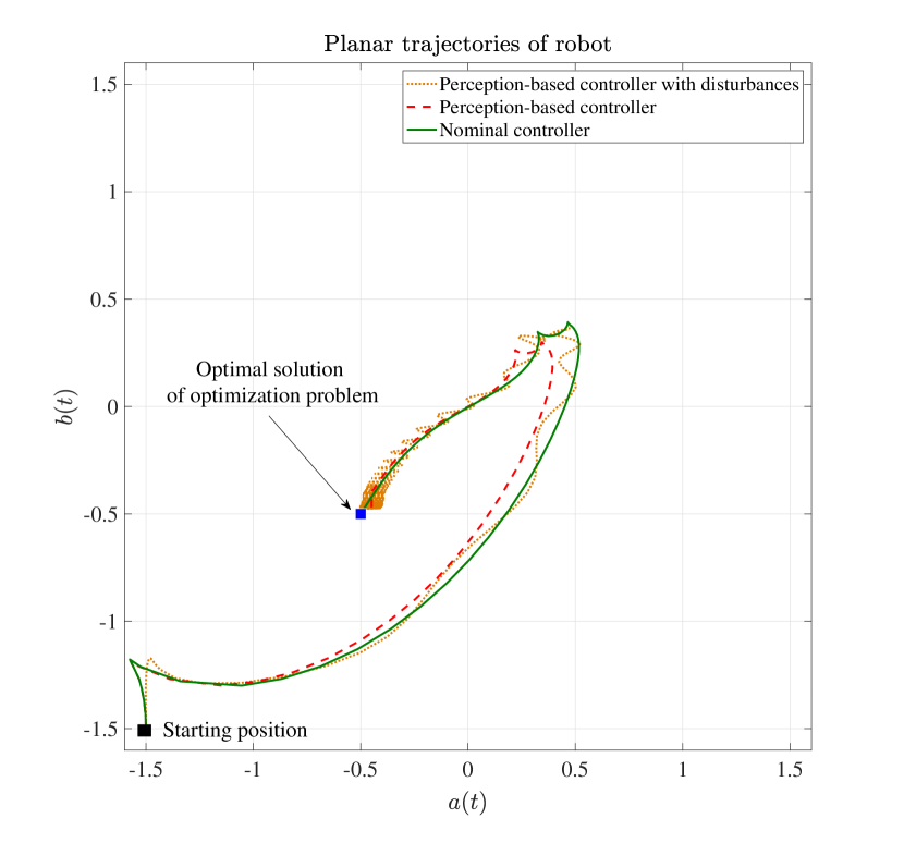
In this section, we illustrate how to apply the proposed framework to control a unicycle robot to track an optimal equilibrium point and whose position is accessible only through camera images. We consider a robot described by unicycle dynamics with state x=(a,b,θ)3,𝑥𝑎𝑏𝜃superscript3x=(a,b,\theta)\in\mathbb{R}^{3}, where r:=(a,b)𝖳2assign𝑟superscript𝑎𝑏𝖳superscript2r:=(a,b)^{\mathsf{T}}\in\mathbb{R}^{2} denotes the position of the robot in a 2-dimensional plane, and θ(π,π]𝜃𝜋𝜋\theta\in(-\pi,\pi] denotes its orientation with respect to the alimit-from𝑎a-axis [45]. The unicycle dynamics are:

a˙˙𝑎\displaystyle\dot{a} =vcos(θ),absent𝑣𝜃\displaystyle=v\cos(\theta), b˙˙𝑏\displaystyle\dot{b} =vsin(θ),absent𝑣𝜃\displaystyle=v\sin(\theta), θ˙˙𝜃\displaystyle\dot{\theta} =ω,absent𝜔\displaystyle=\omega, (20)

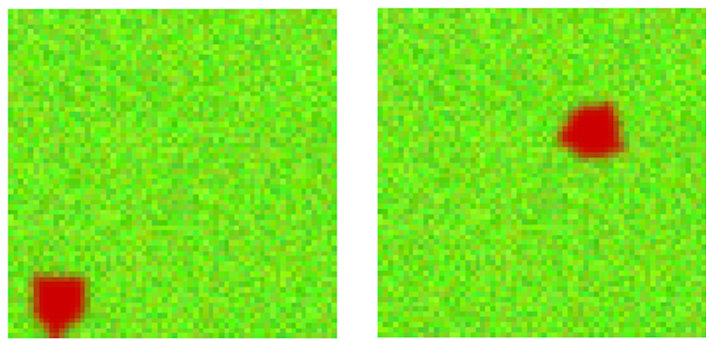
where v,ω𝑣𝜔v,\omega\in\mathbb{R} are the controllable inputs. Given the dynamics (20), we assume that its state x=(a,b,θ)𝑥𝑎𝑏𝜃x=(a,b,\theta) is not directly measurable for control purposes, instead, at every time x𝑥x can be observed only through a noisy camera image, denoted by ξ=q(x)𝜉𝑞𝑥\xi=q(x); see, e.g. [2, 1]. To tackle the desired problem, we consider an instance of (4) with:

ϕ(u)italic-ϕ𝑢\displaystyle\phi(u) =u2,absentsuperscriptnorm𝑢2\displaystyle=\|u\|^{2}, ψ(r)𝜓𝑟\displaystyle\psi(r) =rrf2,absentsuperscriptnorm𝑟superscript𝑟𝑓2\displaystyle=\|r-r^{f}\|^{2},

where rf2superscript𝑟𝑓superscript2r^{f}\in\mathbb{R}^{2} denotes the desired final position of the robot.

To address this problem, we consider a two-level control architecture, where an onboard (low-level) stabilizing controller is first used to stabilize the unicycle dynamics (20) (to guarantee satisfaction of Assumption 3) and, subsequently, the control framework outlined in Algorithm 1 is utilized to select an optimal high-level control references. To design a stabilizing controller, let u=(ua,ub)2𝑢subscript𝑢𝑎subscript𝑢𝑏superscript2u=(u_{a},u_{b})\in\mathbb{R}^{2} denote the instantaneous high-level control input, and consider the standard change of variables from rectangular to polar coordinates (ξ,ϕ)𝜉italic-ϕ(\xi,\phi), given by:

ξ𝜉\displaystyle\xi :=ux,assignabsentnorm𝑢𝑥\displaystyle:=\|u-x\|, ϕitalic-ϕ\displaystyle\phi :=atan(ubbuaa)θ.assignabsentatansubscript𝑢𝑏𝑏subscript𝑢𝑎𝑎𝜃\displaystyle:=\operatorname{atan}\left(\frac{u_{b}-b}{u_{a}-a}\right)-\theta. (21)

In the new variables, the dynamics read as:

ξ˙˙𝜉\displaystyle\dot{\xi} =vcos(ϕ),absent𝑣italic-ϕ\displaystyle=-v\cos(\phi), ϕ˙˙italic-ϕ\displaystyle\dot{\phi} =vξsin(ϕ)ω.absent𝑣𝜉italic-ϕ𝜔\displaystyle=\frac{v}{\xi}\sin(\phi)-\omega. (22)

The following lemma provides a stabilizing control law for (22).

Lemma 6.19.

(Stability of unicycle dynamics) The unicycle dynamics (22) with the following control law:

v𝑣\displaystyle v =kξcos(ϕ),absent𝑘𝜉italic-ϕ\displaystyle=k\xi\cos(\phi), ω𝜔\displaystyle\omega =k(cos(ϕ)+1)sin(ϕ)+kϕ,absent𝑘italic-ϕ1italic-ϕ𝑘italic-ϕ\displaystyle=k(\cos(\phi)+1)\sin(\phi)+k\phi, (23)

k>0𝑘0k>0, admit a unique equilibrium point (ξ,ϕ)=(0,0)𝜉italic-ϕ00(\xi,\phi)=(0,0) that is globally exponentially stable.

Proof 6.20.

Noticing that the dynamics of ξ𝜉\xi and ϕitalic-ϕ\phi are decoupled, consider the Lyapunov function V(ϕ)=12ϕ2𝑉italic-ϕ12superscriptitalic-ϕ2V(\phi)=\frac{1}{2}\phi^{2}. We have:

V˙(ϕ)=kϕsin(ϕ)kϕ2kϕ2=2kV(ϕ),˙𝑉italic-ϕ𝑘italic-ϕitalic-ϕ𝑘superscriptitalic-ϕ2𝑘superscriptitalic-ϕ22𝑘𝑉italic-ϕ\displaystyle\dot{V}(\phi)=-k\phi\sin(\phi)-k\phi^{2}\leq-k\phi^{2}=-2kV(\phi),

with V(ϕ)=0𝑉italic-ϕ0V(\phi)=0 if and only if ϕ=0italic-ϕ0\phi=0. The proof of exponential stability of ξ𝜉\xi follows immediately from [45, Lem. 2.1].

According to Lemma 6.19, the dynamics (22) with the on-board control law (23) satisfy Assumption 3. We next apply the perception-based control framework outlined in Algorithm 2 to design the reference input u𝑢u to be utilized in (21).

Refer to caption
Refer to caption
Figure 4: Numerical validation of Algorithm 1. The technique is used to control a robot whose state (a,b,θ)𝑎𝑏𝜃(a,b,\theta) cannot be directly measured and is instead estimated using a residual neural network from aerial images. (a) Trajectory of the robot (in the coordinates (a,b)𝑎𝑏(a,b)) with the perception-based controller and with a nominal controller using perfect state information. (b) Images that the perception-based controller uses at t=4.32𝑡4.32t=4.32 seconds (left image) and t=70.36𝑡70.36t=70.36 seconds (right image).

For our perception-based controller, we use a residual neural network to estimate the state perception map; in particular, the neural network returns estimated state coordinates from aerial images following the procedure of Algorithm 2. To prepare for the execution of Algorithm 2, we generate 122,880122880122,880 square, blurry, RGB images of size 64×64646464\times 64 pixels to represent the location and orientation of the robot on a two-dimensional plane. These images were built using the MATLAB Image Processing Toolbox. First, we build a base image of a maroon pentagon representing the robot over a grassy background (using ranges of RGB values for different green colors), and then add blurriness to the image using the MATLAB function imgaussfilt; see, for example, the sample images in Figure 4(b). This function filters the base image with a 2-D Gaussian smoothing kernel with a standard deviation of 0.50.50.5. For our residual network, we used the resnet50 network structure given in the MATLAB Deep Learning Toolbox and tailored the input output sizes for our particular setting. Specifically, we set the input layer to read in images of size 64×64646464\times 64 pixels and set the number of possible output labels as 642=4996superscript642499664^{2}=4996 to account for all possible locations or coordinates of the pixelized image. The number of training images for the network was chosen so that all possible locations or coordinates of the pixelized image are generated for 30 different orientations, totaling 122,880122880122,880 training images. After training, the residual network returns estimated locations in the 2D plane by identifying the center pixel of the robot. Of course, during the time-evolution of the closed loop dynamics with the residual network, the returned labels are converted into (a,b)𝑎𝑏(a,b) coordinates.

Simulation results are presented in Figure 4, when using the initial conditions (a0,b0,θ0,ua0,ub0)=(1.5,1.5,π/2,1,1)subscript𝑎0subscript𝑏0subscript𝜃0subscript𝑢subscript𝑎0subscript𝑢subscript𝑏01.51.5𝜋211(a_{0},b_{0},\theta_{0},u_{a_{0}},u_{b_{0}})=(-1.5,-1.5,-\pi/2,1,1); moreover, the optimal solution of the problem is r=(0.5,0.5)superscript𝑟0.50.5r^{*}=(-0.5,-0.5). As evidenced in Figure  4(a), differences persist between the trajectories produced by the nominal controller, which utilizes perfect state information, and by the perception-based controller. Importantly, imperfect estimates of (a,b)𝑎𝑏(a,b) are also due to the fact that the labels returned from our trained network correspond to the pixels of the image, which can limit how well the (a,b)𝑎𝑏(a,b) values are represented. Figure 4(b) shows sample images at times t=4.32𝑡4.32t=4.32 and t=70.36𝑡70.36t=70.36; these images are used as inputs to the neural network. As expected, the ideal controller converges to the reference state arbitrarily well, while the perception-based controller converges to the reference state to within a neighborhood dependent on the error associated with the perceived state. Overall, these simulations demonstrate the claims made in Proposition 4.10.

7 Application to epidemic control

In this section, we apply the proposed framework to regulate the spread of an epidemic by controlling contact-relevant transmissions. The latter is achieved by e.g. selecting the intensity of restrictions such as mask-wearing, social restrictions, school closures, and stay-at-home orders, etc. To describe the epidemic evolution, we adopt a susceptible-infected-susceptible (SIS) model [58], described by:

s˙˙𝑠\displaystyle\dot{s} =μμsuβsx+γx,absent𝜇𝜇𝑠𝑢𝛽𝑠𝑥𝛾𝑥\displaystyle=\mu-\mu s-u\beta sx+\gamma x, x˙˙𝑥\displaystyle\dot{x} =uβsx(γ+μ)x,absent𝑢𝛽𝑠𝑥𝛾𝜇𝑥\displaystyle=u\beta sx-(\gamma+\mu)x, (24)

where s,xformulae-sequence𝑠𝑥s\in\mathbb{R},x\in\mathbb{R} describe the fraction of susceptible and infected population, respectively, with s+x=1𝑠𝑥1s+x=1 at all times, u(0,1]𝑢01u\in(0,1] is an input modeling the reduction in contact-relevant transmissions, β>0𝛽0\beta>0 is the transmission rate, μ>0𝜇0\mu>0 is the death/birth rate, and γ>0𝛾0\gamma>0 is the recovery rate. Model parameters of (24) are chosen as follows: β=4𝛽4\beta=4, γ=1/9𝛾19\gamma=1/9, μ=104𝜇superscript104\mu=10^{-4}, cost function parameters: uref=0.36superscript𝑢ref0.36{u}^{\textup{ref}}=0.36, xref=0.85superscript𝑥ref0.85{x}^{\textup{ref}}=0.85, wψ=wψ=1subscript𝑤𝜓subscript𝑤𝜓1w_{\psi}=w_{\psi}=1. As characterized in [58, Thm. 2.1 and Lem. 2.1], (24) admits a unique (unstable) equilibrium point described by x=0𝑥0x=0 (called disease-free equilibrium) and a unique equilibrium point with x0𝑥0x\neq 0 (called endemic equilibrium) that is exponentially stable [58, Thm. 2.4], thus satisfying Assumption 3. We utilize the control problem (4) to determine an optimal balance between a desired fraction of infections xrefsuperscript𝑥ref{x}^{\textup{ref}} and a desired level of restrictions urefsuperscript𝑢ref{u}^{\textup{ref}}. More formally, we consider an instance of (4) with ϕ(u)=wϕ(uuref)2italic-ϕ𝑢subscript𝑤italic-ϕsuperscript𝑢superscript𝑢ref2\phi(u)=w_{\phi}(u-{u}^{\textup{ref}})^{2} and ψ(x)=wψ(xxref)2𝜓𝑥subscript𝑤𝜓superscript𝑥superscript𝑥ref2\psi(x)=w_{\psi}(x-{x}^{\textup{ref}})^{2}, where uref,xref[0,1]superscript𝑢refsuperscript𝑥ref01{u}^{\textup{ref}},{x}^{\textup{ref}}\in[0,1] are desired reference inputs and states and wϕ,wψ0subscript𝑤italic-ϕsubscript𝑤𝜓subscriptabsent0w_{\phi},w_{\psi}\in\mathbb{R}_{\geq 0} are weighting factors. For our simulations, we perform the change of variables (x~,u~)=(x,1u)~𝑥~𝑢𝑥1𝑢(\tilde{x},\tilde{u})=(x,\frac{1}{u}); in the new variables, h(u~)=1μ+γβu~~𝑢1𝜇𝛾𝛽~𝑢h(\tilde{u})=1-\frac{\mu+\gamma}{\beta}\tilde{u} satisfies Assumptions 1 and 4. In order to illustrate the effects of perception on the control loops, in what follows we assume wt=0subscript𝑤𝑡0w_{t}=0 so all the tracking error can be associated to perception errors.

7.1 Optimization with State Perception

We begin by illustrating the case of state perception (Section 4). One of the main challenges in predicting and controlling the outbreak of an epidemic is related to the difficulty in estimating the true number of infections from incomplete information describing documented infected individuals with symptoms severe enough to be confirmed. During the outbreak of COVID-19, researchers have proposed several methods to overcome these challenges and by using several sources of data including [59] detected cases, recovered cases, deaths, test positivity [60], and mobility data [61, 46]. In our simulations, we adopted the approach in Algorithm 1 to achieve this task. For the purpose of illustration, we utilized a map q()𝑞q(\cdot) composed of a set of 444 Gaussian basis functions with mean μb=(1,5,9,13)subscript𝜇b15913{\mu}_{\textup{b}}=(1,5,9,13) and variance σ=I𝜎𝐼\sigma=I to determine the perception signal ξ𝜉\xi. The training phase of Algorithm 1 has then been performed using a feedforward neural network to determine the map x^=p^(ξ)^𝑥^𝑝𝜉\hat{x}=\hat{p}(\xi) to reconstruct the state of (24). Simulation results are illustrated in Figure 5. As illustrated by the state trajectories in Figure 5(a)-(b), the use of a neural network originates discrepancies between the true state and the estimated state, especially during transient phases. Figure 5(c) provides a comparison of the tracking error between the use of the ideal controller (6) (which uses the exact state) and the controller in Algorithm 1. The numerics illustrate that while the exact controller (6) is capable of converging to the desired optimizer with arbitrary accuracy, the controller in Algorithm 1 yields an error of the order 102superscript10210^{-2}, due to uncertainties in the reconstructed system state. Overall, the simulations validate the convergence claim made in Proposition 4.14.
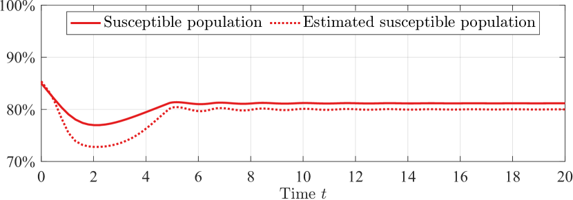
Refer to caption
Refer to caption
Refer to caption
Figure 5: Numerical validation of Algorithm 1. The technique is used to control an epidemic SIS model whose state cannot be directly measured and is instead reconstructed using a neural network. Panels (a)-(b) compare the time-evolution of the true states and of the estimated states. Panel (c) compares the performance of the ideal controller (6) with that of the perception-based counterpart described in Algorithm 1. Steady-state errors in Algorithm 1 are associated to errors originated by the use of a neural network (see Proposition 4.14).

7.2 Optimization with Cost-Function Perception

Next, we illustrate the case of cost perception (Section 5). For illustration purposes, we focus on cases where the analytic expression of ϕ(u)italic-ϕ𝑢\phi(u) in (4) is known, while ψ(x)𝜓𝑥\psi(x) is unknown. As described in Algorithm 2, we utilized a set of samples {(xi,ψ(xi))}i=1Msuperscriptsubscriptsubscript𝑥𝑖𝜓subscript𝑥𝑖𝑖1𝑀\{(x_{i},\psi(x_{i}))\}_{i=1}^{M} to train a feedforward neural network to approximate the function ψ(x)𝜓𝑥\psi(x). Simulation results are illustrated in Figure 6. Figure 6(a) illustrates the set of samples used for training and provides a comparison between the true gradient ψ(x)𝜓𝑥\nabla\psi(x) and the approximate gradient gx(x)subscript𝑔𝑥𝑥g_{x}(x), obtained through the neural network. Figure 6(b) provides a comparison between the state trajectories obtained by using the ideal controller (6) and those obtained through the perception-based controller in Algorithm 2. Figure 5(c) provides a comparison of the tracking error between the use of the ideal controller (6) (which uses the exact gradients of the cost) and the controller in Algorithm 2. The simulations illustrate that while the exact controller (6) is capable of converging to the desired optimizer with arbitrary accuracy, the controller in Algorithm 2 yields a nontrivial steady-state error due to uncertainties in the gradient function. Overall, the simulations validate the convergence claim made in Proposition 5.16.
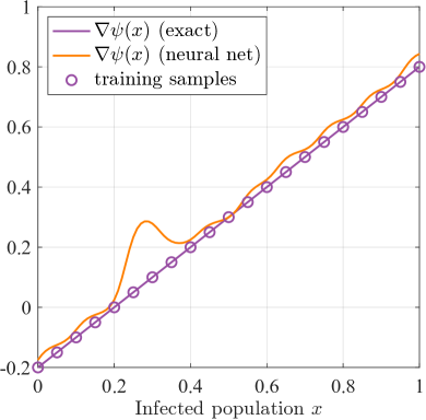
Refer to caption
Refer to caption
Refer to caption
Figure 6: Numerical validation of Algorithm 2. The technique is used to control an epidemic SIS model, where the economic impact of infections is unknown and must be estimated from samples using a neural network. Panel (a) illustrates the approximation accuracy of the neural network (used to approximate the gradient of the function). Panel (b) compares the time-evolution of the true states obtained by using Algorithm 2 and those obtained by using the ideal controller (6). Panel (c) compares the tracking error of the ideal and perception-based control methods. Steady-state errors in Algorithm 2 are associated to errors originated by the use of a neural network to compute the gradients (see Proposition 5.16).

8 Conclusions

We proposed algorithms to control and optimize dynamical systems when the system state cannot be measured and the cost functions in the optimization are unknown, instead, these quantities can only be sensed via neural network-based perception. Our results show for the first time how feedback-based optimizing controllers can be adapted to operate with perception in the control loop. Our findings crucially hinge on recent results on the uniform approximation properties of deep neural networks. We believe that the results can be further refined to account for cases where the training of the neural networks is performed online and we are currently investigating such possibility. While this paper provided conditions to obtain exponential ISS results for the interconnection of a plant with a projected gradient-flow controller, future efforts will analyze the interconnection of plants and controllers that are (locally) asymptotically stable when taken individually.

[Proof of Theorem 3.7]

The proof of this claim uses Lyapunov-based singular perturbation reasonings, and is organized into seven main steps.

(1 – Change of variables) We consider the change of variables x~=xh(u,w)~𝑥𝑥𝑢𝑤\tilde{x}=x-h(u,w), which shift the equilibrium of (1) to the origin. In the new variables, (7) reads as:

x~˙˙~𝑥\displaystyle\dot{\tilde{x}} =f(x~+h(u,w),u,w)ddth(u,w),absent𝑓~𝑥𝑢𝑤𝑢𝑤𝑑𝑑𝑡𝑢𝑤\displaystyle=f(\tilde{x}+h(u,w),u,w)-\frac{d}{dt}{h}(u,w), (25a)
u˙˙𝑢\displaystyle\dot{u} =Π𝒞{uη(F~(x~,u)+e(x~+h(u,wt),u)}u,\displaystyle=\Pi_{\mathcal{C}}\{u-\eta(\tilde{F}(\tilde{x},u)+e(\tilde{x}+h(u,w_{t}),u)\}-u, (25b)

where we denoted, in compact form, F~(x~,u):=F(x~+h(u,w),u)assign~𝐹~𝑥𝑢𝐹~𝑥𝑢𝑤𝑢\tilde{F}(\tilde{x},u):=F(\tilde{x}+h(u,w),u), e~(x~,u):=e(x~+h(u,wt),u)assign~𝑒~𝑥𝑢𝑒~𝑥𝑢subscript𝑤𝑡𝑢\tilde{e}(\tilde{x},u):=e(\tilde{x}+h(u,w_{t}),u). Before proceeding, we note that:

F~(x~,u)F~(0,ut)norm~𝐹~𝑥𝑢~𝐹0superscriptsubscript𝑢𝑡\displaystyle\|\tilde{F}(\tilde{x},u)-\tilde{F}(0,u_{t}^{*})\| F~(x~,u)F~(0,u)+absentlimit-fromnorm~𝐹~𝑥𝑢~𝐹0𝑢\displaystyle\leq\|\tilde{F}(\tilde{x},u)-\tilde{F}(0,u)\|+
F~(0,u)F~(0,ut)norm~𝐹0𝑢~𝐹0superscriptsubscript𝑢𝑡\displaystyle\quad\quad\quad\quad\quad\|\tilde{F}(0,u)-\tilde{F}(0,u_{t}^{*})\|
huyx~+uut,absentsubscriptsubscript𝑢subscript𝑦norm~𝑥norm𝑢superscriptsubscript𝑢𝑡\displaystyle\leq\ell_{h_{u}}\ell_{y}\|\tilde{x}\|+\ell\|u-u_{t}^{*}\|, (26)

where we recall that (hu,y,)subscriptsubscript𝑢subscript𝑦(\ell_{h_{u}},\ell_{y},\ell) are as in Assump. 1 and 4(a).

(2 – Lyapunov functions) Inspired by singular perturbation reasonings [31, Ch. 11], we adopt the following composite Lyapunov function for (25):

ν(x~,u,t):=θ1ηW(x~,u,wt)+(1θ)1ηV(u,ut),assign𝜈~𝑥𝑢𝑡𝜃1𝜂𝑊~𝑥𝑢subscript𝑤𝑡1𝜃1𝜂𝑉𝑢superscriptsubscript𝑢𝑡\displaystyle\nu(\tilde{x},u,t):=\theta\frac{1}{\eta}W(\tilde{x},u,w_{t})+(1-\theta)\frac{1}{\eta}V(u,u_{t}^{*}), (27)

where θ𝜃\theta is as defined in (3), W(x~,u,w)𝑊~𝑥𝑢𝑤W(\tilde{x},u,w) describes a Lyapunov function for (25a) and is given in Lemma 1, and V(u,ut)𝑉𝑢superscriptsubscript𝑢𝑡V(u,u_{t}^{*}) describes a Lyapunov function for (25b) and is given by: V(u,ut)=12uut2𝑉𝑢superscriptsubscript𝑢𝑡12superscriptnorm𝑢superscriptsubscript𝑢𝑡2V(u,u_{t}^{*})=\frac{1}{2}\|u-u_{t}^{*}\|^{2}.

Before proceeding, we notice that ν(x~,u,t)𝜈~𝑥𝑢𝑡\nu(\tilde{x},u,t) satisfies

c1(x~,uut)2ν(x~,u,t)c2(x~,uut)2,subscript𝑐1superscriptnorm~𝑥𝑢superscriptsubscript𝑢𝑡2𝜈~𝑥𝑢𝑡subscript𝑐2superscriptnorm~𝑥𝑢superscriptsubscript𝑢𝑡2\displaystyle c_{1}\|(\tilde{x},u-u_{t}^{*})\|^{2}\leq\nu(\tilde{x},u,t)\leq c_{2}\|(\tilde{x},u-u_{t}^{*})\|^{2},

where c1,c2subscript𝑐1subscript𝑐2c_{1},c_{2} are as in (3).

(3 – Bound for the Time-Derivative of W𝑊W) We begin by bounding the time-derivative ddtW𝑑𝑑𝑡𝑊\frac{d}{dt}W. To this end, notice that Lemma 1 guarantees the following estimates:

Wx~f(x~+h(u,w),u,w)d3x~2,𝑊~𝑥𝑓~𝑥𝑢𝑤𝑢𝑤subscript𝑑3superscriptnorm~𝑥2\displaystyle\frac{\partial W}{\partial\tilde{x}}f(\tilde{x}+h(u,w),u,w)\leq-d_{3}\|\tilde{x}\|^{2},
Wx~ddth(u,w)=Wx~(uh(u,w)u˙+wh(u,w)w˙)𝑊~𝑥𝑑𝑑𝑡𝑢𝑤𝑊~𝑥subscript𝑢𝑢𝑤˙𝑢subscript𝑤𝑢𝑤˙𝑤\displaystyle\frac{\partial W}{\partial\tilde{x}}\frac{d}{dt}{h}(u,w)=\frac{\partial W}{\partial\tilde{x}}\left(\nabla_{u}h(u,w)\dot{u}+\nabla_{w}h(u,w)\dot{w}\right)
d4x~(huu˙+hww˙).absentsubscript𝑑4norm~𝑥subscriptsubscript𝑢norm˙𝑢subscriptsubscript𝑤norm˙𝑤\displaystyle\quad\quad\quad\quad\quad\quad\leq d_{4}\|\tilde{x}\|(\ell_{h_{u}}\|\dot{u}\|+\ell_{h_{w}}\|\dot{w}\|).

By using the above estimates and Lemma 1, we have:

ddtW(x~,u,w)𝑑𝑑𝑡𝑊~𝑥𝑢𝑤\displaystyle\frac{d}{dt}W(\tilde{x},u,w) d3x~2+(d4hu+d5)u˙x~absentsubscript𝑑3superscriptnorm~𝑥2subscript𝑑4subscriptsubscript𝑢subscript𝑑5norm˙𝑢norm~𝑥\displaystyle\leq-d_{3}\|\tilde{x}\|^{2}+(d_{4}\ell_{h_{u}}+d_{5})\|\dot{u}\|\|\tilde{x}\|
+(d4hw+d6)w˙tx~.subscript𝑑4subscriptsubscript𝑤subscript𝑑6normsubscript˙𝑤𝑡norm~𝑥\displaystyle\quad\quad+(d_{4}\ell_{h_{w}}+d_{6})\|\dot{w}_{t}\|\|\tilde{x}\|.

Next, refine the bound on the second term. Notice that

u˙norm˙𝑢\displaystyle\|\dot{u}\| =Π𝒞{uηF~(x~,u)+ηe~(x~,u)}uabsentnormsubscriptΠ𝒞𝑢𝜂~𝐹~𝑥𝑢𝜂~𝑒~𝑥𝑢𝑢\displaystyle=\|\Pi_{\mathcal{C}}\left\{u-\eta\tilde{F}(\tilde{x},u)+\eta\tilde{e}(\tilde{x},u)\right\}-u\|
ηF~(x~,u)F~(0,ut)+ηe~(x~,u)absent𝜂norm~𝐹~𝑥𝑢~𝐹0superscriptsubscript𝑢𝑡𝜂norm~𝑒~𝑥𝑢\displaystyle\leq\eta\|\tilde{F}(\tilde{x},u)-\tilde{F}(0,u_{t}^{*})\|+\eta\|\tilde{e}(\tilde{x},u)\|
=ηhuyx~+ηuut+ηe~(x~,u).absent𝜂subscriptsubscript𝑢subscript𝑦norm~𝑥𝜂norm𝑢superscriptsubscript𝑢𝑡𝜂norm~𝑒~𝑥𝑢\displaystyle=\eta\ell_{h_{u}}\ell_{y}\|\tilde{x}\|+\eta\ell\|u-u_{t}^{*}\|+\eta\|\tilde{e}(\tilde{x},u)\|.

To obtain the first inequality, add uΠ𝒞{uηF~(0,u)}=0superscript𝑢subscriptΠ𝒞superscript𝑢𝜂~𝐹0superscript𝑢0u^{*}-\Pi_{\mathcal{C}}\{u^{*}-\eta\tilde{F}(0,u^{*})\}=0 and apply the triangle inequality. Then, apply the bounds obtained in (8). It follows that

ddtW(x~,u,w)d3x~2+ηhuy(d4hu+d5)x~2𝑑𝑑𝑡𝑊~𝑥𝑢𝑤subscript𝑑3superscriptnorm~𝑥2𝜂subscriptsubscript𝑢subscript𝑦subscript𝑑4subscriptsubscript𝑢subscript𝑑5superscriptnorm~𝑥2\displaystyle\frac{d}{dt}W(\tilde{x},u,w)\leq-d_{3}\|\tilde{x}\|^{2}+\eta\ell_{h_{u}}\ell_{y}(d_{4}\ell_{h_{u}}+d_{5})\|\tilde{x}\|^{2}
+η(d4hu+d5)uux~𝜂subscript𝑑4subscriptsubscript𝑢subscript𝑑5norm𝑢superscript𝑢norm~𝑥\displaystyle\quad+\eta\ell(d_{4}\ell_{h_{u}}+d_{5})\|u-u^{*}\|\|\tilde{x}\| (28)
+η(d4hu+d5)e(x~,u)x~+(d4hw+d6)w˙tx.𝜂subscript𝑑4subscriptsubscript𝑢subscript𝑑5norm𝑒~𝑥𝑢norm~𝑥subscript𝑑4subscriptsubscript𝑤subscript𝑑6normsubscript˙𝑤𝑡norm𝑥\displaystyle\quad+\eta(d_{4}\ell_{h_{u}}+d_{5})\|e(\tilde{x},u)\|\|\tilde{x}\|+(d_{4}\ell_{h_{w}}+d_{6})\|\dot{w}_{t}\|\|x\|.

(4 – Bound for the Time-Derivative of V𝑉V) Next, we bound the time-derivative ddtV𝑑𝑑𝑡𝑉\frac{d}{dt}V. In what follows, we use the compact notation u~:=uutassign~𝑢𝑢superscriptsubscript𝑢𝑡\tilde{u}:=u-u_{t}^{*}. By expanding:

ddtV(u,ut)=u~u˙u~u˙tu~u˙+Jw˙u~,𝑑𝑑𝑡𝑉𝑢superscriptsubscript𝑢𝑡superscript~𝑢top˙𝑢superscript~𝑢topsuperscriptsubscript˙𝑢𝑡superscript~𝑢top˙𝑢subscript𝐽delimited-∥∥˙𝑤delimited-∥∥~𝑢\displaystyle\begin{split}\frac{d}{dt}V(u,u_{t}^{*})&=\tilde{u}^{\top}\dot{u}-\tilde{u}^{\top}\dot{u}_{t}^{*}\leq\tilde{u}^{\top}\dot{u}+\ell_{J}\|\dot{w}\|\|\tilde{u}\|,\end{split} (29)

where we used Assumption 5. The first term above satisfies:

u~u˙superscript~𝑢top˙𝑢\displaystyle\tilde{u}^{\top}\dot{u} u~𝖳(Π𝒞{uηF~(0,u)}u)absentsuperscript~𝑢𝖳subscriptΠ𝒞𝑢𝜂~𝐹0𝑢𝑢\displaystyle\leq\tilde{u}^{\mathsf{T}}(\Pi_{\mathcal{C}}\{u-\eta\tilde{F}(0,u)\}-u) (30)
+ηhux~u~+ηu~e~(x~,u).𝜂subscriptsubscript𝑢norm~𝑥norm~𝑢𝜂norm~𝑢norm~𝑒~𝑥𝑢\displaystyle\quad\quad\quad+\eta\ell_{h_{u}}\ell\|\tilde{x}\|\|\tilde{u}\|+\eta\|\tilde{u}\|\|\tilde{e}(\tilde{x},u)\|.

To obtain (30), we added and subtracted Π𝒞{uηF(0,u)}subscriptΠ𝒞𝑢𝜂𝐹0𝑢\Pi_{\mathcal{C}}\{u-\eta F(0,u)\}, we applied the triangle inequality, and we used Assumptions 1 and 4(a). Next, we use the fact that the first term on the right hand side of (30) satisfies:

u~(Puu)η(μη2/4)u~2.superscript~𝑢topsubscript𝑃𝑢𝑢𝜂𝜇𝜂superscript24superscriptnorm~𝑢2\displaystyle\tilde{u}^{\top}\left(P_{u}-u\right)\leq-\eta\left(\mu-\eta\ell^{2}/4\right)\|\tilde{u}\|^{2}. (31)

(This fact will be proven in Step 5, shortly below.) By combining (29)-(30)-(31) we conclude that:

ddtV𝑑𝑑𝑡𝑉\displaystyle\frac{d}{dt}V η(μη24)u~2+ηhux~u~absent𝜂𝜇𝜂superscript24superscriptnorm~𝑢2𝜂subscriptsubscript𝑢norm~𝑥norm~𝑢\displaystyle\leq-\eta\left(\mu-\eta\frac{\ell^{2}}{4}\right)\|\tilde{u}\|^{2}+\eta\ell_{h_{u}}\ell\|\tilde{x}\|\|\tilde{u}\|
+ηu~e(x~,u)+Jw˙u~.𝜂norm~𝑢norm𝑒~𝑥𝑢subscript𝐽norm˙𝑤norm~𝑢\displaystyle\quad\quad+\eta\|\tilde{u}\|\|e(\tilde{x},u)\|+\ell_{J}\|\dot{w}\|\|\tilde{u}\|. (32)

(5 – Proof of (31)) For brevity, in what follows we use the compact notation Pu:=Π𝒞{uηF~(0,u)}.assignsubscript𝑃𝑢subscriptΠ𝒞𝑢𝜂~𝐹0𝑢P_{u}:=\Pi_{\mathcal{C}}\{u-\eta\tilde{F}(0,u)\}. To prove (31), we recall the following property of the projection operator:

(uΠ𝒞(v))(Π𝒞(v)v)0,u𝒞,formulae-sequencesuperscriptsuperscript𝑢subscriptΠ𝒞𝑣topsubscriptΠ𝒞𝑣𝑣0for-allsuperscript𝑢𝒞\left(u^{\prime}-\Pi_{\mathcal{C}}(v)\right)^{\top}\left(\Pi_{\mathcal{C}}(v)-v\right)\geq 0,~{}~{}\forall~{}u^{\prime}\in\mathcal{C},

which holds for any vnu𝑣superscriptsubscript𝑛𝑢v\in\mathcal{\mathbb{R}}^{n_{u}}. By applying this property with u:=utassignsuperscript𝑢superscriptsubscript𝑢𝑡u^{\prime}:=u_{t}^{*} and v=uηF~(0,u)𝑣𝑢𝜂~𝐹0𝑢v=u-\eta\tilde{F}(0,u), we have:

(utPu)(Puu+ηF~(0,u))0.superscriptsuperscriptsubscript𝑢𝑡subscript𝑃𝑢topsubscript𝑃𝑢𝑢𝜂~𝐹0𝑢0\left(u_{t}^{*}-P_{u}\right)^{\top}(P_{u}-u+\eta\tilde{F}(0,u))\geq 0.

By expanding and by adding u(uPu+ηF~(0,u))superscript𝑢top𝑢subscript𝑃𝑢𝜂~𝐹0𝑢u^{\top}(u-P_{u}+\eta\tilde{F}(0,u)) to both sides of the inequality, the left hand side reads as:

uuuPuutu+utPu+ηuF~(0,u)ηF~(0,u)Pu,superscript𝑢top𝑢superscript𝑢topsubscript𝑃𝑢superscriptsubscript𝑢𝑡absenttop𝑢superscriptsubscript𝑢𝑡absenttopsubscript𝑃𝑢𝜂superscript𝑢top~𝐹0𝑢𝜂~𝐹superscript0𝑢topsubscript𝑃𝑢u^{\top}u-u^{\top}P_{u}-u_{t}^{*\top}u+u_{t}^{*\top}P_{u}+\eta u^{\top}\tilde{F}(0,u)-\eta\tilde{F}(0,u)^{\top}P_{u},

while the right hand side reads as:

uuPuuuPu+PuPu+ηuF~(0,u)ηutF~(u,0),superscript𝑢top𝑢superscriptsubscript𝑃𝑢top𝑢superscript𝑢topsuperscriptsubscript𝑃𝑢topsuperscriptsubscript𝑃𝑢topsubscript𝑃𝑢𝜂superscript𝑢top~𝐹0𝑢𝜂superscriptsubscript𝑢𝑡superscripttop~𝐹𝑢0u^{\top}u-P_{u}^{\top}u-u^{\top}P_{u}^{\top}+P_{u}^{\top}P_{u}+\eta u^{\top}\tilde{F}(0,u)-\eta u_{t}^{*^{\top}}\tilde{F}(u,0),

and, after regrouping,

u~(uPu)uPu2+η(Puut)F~(u,0).superscript~𝑢top𝑢subscript𝑃𝑢superscriptnorm𝑢subscript𝑃𝑢2𝜂superscriptsubscript𝑃𝑢superscriptsubscript𝑢𝑡top~𝐹𝑢0\displaystyle\tilde{u}^{\top}\left(u-P_{u}\right)\geq\|u-P_{u}\|^{2}+\eta(P_{u}-u_{t}^{*})^{\top}\tilde{F}(u,0).

By adding and subtracting η(Puut)F~(0,ut)𝜂superscriptsubscript𝑃𝑢superscriptsubscript𝑢𝑡top~𝐹0superscriptsubscript𝑢𝑡\eta\left(P_{u}-u_{t}^{*}\right)^{\top}\tilde{F}(0,u_{t}^{*}):

u~(Puu)superscript~𝑢topsubscript𝑃𝑢𝑢\displaystyle\tilde{u}^{\top}(P_{u}-u) uPu2η(Puut)F~(ut,0)absentsuperscriptnorm𝑢subscript𝑃𝑢2𝜂superscriptsubscript𝑃𝑢superscriptsubscript𝑢𝑡top~𝐹superscriptsubscript𝑢𝑡0\displaystyle\leq-\|u-P_{u}\|^{2}-\eta(P_{u}-u_{t}^{*})^{\top}\tilde{F}(u_{t}^{*},0)
η(Puut)(F~(0,u)F~(0,ut)).𝜂superscriptsubscript𝑃𝑢superscriptsubscript𝑢𝑡top~𝐹0𝑢~𝐹0superscriptsubscript𝑢𝑡\displaystyle\quad-\eta(P_{u}-u_{t}^{*})^{\top}(\tilde{F}(0,u)-\tilde{F}(0,u_{t}^{*})).

From this, expand (Puut)=uPuu~subscript𝑃𝑢superscriptsubscript𝑢𝑡𝑢subscript𝑃𝑢~𝑢-(P_{u}-u_{t}^{*})=u-P_{u}-\tilde{u} and apply (Puut)F~(0,u)0.superscriptsubscript𝑃𝑢superscriptsubscript𝑢𝑡top~𝐹0𝑢0\left(P_{u}-u_{t}^{*}\right)^{\top}\tilde{F}(0,u)\geq 0. Use strong convexity and Lipschitz-continuity to obtain,

u~(Puu)superscript~𝑢topsubscript𝑃𝑢𝑢\displaystyle\tilde{u}^{\top}\left(P_{u}-u\right) uPu2ημu~2+ηuPuu~absentsuperscriptnorm𝑢subscript𝑃𝑢2𝜂𝜇superscriptnorm~𝑢2𝜂norm𝑢subscript𝑃𝑢norm~𝑢\displaystyle\leq-\|u-P_{u}\|^{2}-\eta\mu\|\tilde{u}\|^{2}+\eta\ell\|u-P_{u}\|\|\tilde{u}\|
η(μη2/4)u~2,absent𝜂𝜇𝜂superscript24superscriptnorm~𝑢2\displaystyle\leq-\eta\left(\mu-\eta\ell^{2}/4\right)\|\tilde{u}\|^{2},

where the second inequality follows by recalling that, for real numbers a,b𝑎𝑏a,b, it holds 2ab<a2+b22𝑎𝑏superscript𝑎2superscript𝑏22ab<a^{2}+b^{2}, and by letting a=uPu𝑎norm𝑢subscript𝑃𝑢a=\|u-P_{u}\| and b=12ηu~𝑏12𝜂norm~𝑢b=\frac{1}{2}\eta\ell\|\tilde{u}\|. Hence, (31) is proved.

(6 – Conditions for Exponential Convergence) By combining (8) and (8):

ddtν𝑑𝑑𝑡𝜈\displaystyle\frac{d}{dt}\nu (1θ){(μη24)u~2+e~(x~,u)u~\displaystyle\leq(1-\theta)\{-\left(\frac{\mu-\eta\ell^{2}}{4}\right)\|\tilde{u}\|^{2}+\|\tilde{e}(\tilde{x},u)\|\|\tilde{u}\| (33)
+Jηw˙tu~+hux~u~}\displaystyle~{}~{}+\frac{\ell_{J}}{\eta}\|\dot{w}_{t}\|\|\tilde{u}\|+\ell_{h_{u}}\ell\|\tilde{x}\|\|\tilde{u}\|\}
+θ{d3ηx~2+huy(d4hu+d5)x~2\displaystyle~{}~{}+\theta\{-\frac{d_{3}}{\eta}\|\tilde{x}\|^{2}+\ell_{h_{u}}\ell_{y}(d_{4}\ell_{h_{u}}+d_{5})\|\tilde{x}\|^{2}
+(d4hu+d5)u~x~subscript𝑑4subscriptsubscript𝑢subscript𝑑5norm~𝑢norm~𝑥\displaystyle\quad+\ell(d_{4}\ell_{h_{u}}+d_{5})\|\tilde{u}\|\|\tilde{x}\|
+(d4hu+d5)e~(x~,u)+(d4hw+d6)ηw˙tx}.\displaystyle\quad+(d_{4}\ell_{h_{u}}+d_{5})\|\tilde{e}(\tilde{x},u^{\prime})\|+\frac{(d_{4}\ell_{h_{w}}+d_{6})}{\eta}\|\dot{w}_{t}\|\|x^{\prime}\|\}.

By using (10), we have η<2μ2𝜂2𝜇superscript2\eta<\frac{2\mu}{\ell^{2}}, and thus the first term satisfies (η24μ)u~2μ2u~2𝜂superscript24𝜇superscriptnorm~𝑢2𝜇2superscriptnorm~𝑢2(\frac{\eta\ell^{2}}{4}-\mu)\|\tilde{u}\|^{2}\leq-\frac{\mu}{2}\|\tilde{u}\|^{2}. Next, let s(0,1)𝑠01s\in(0,1) be a fixed constant. Then, (33) can be rewritten as:

ddtν𝑑𝑑𝑡𝜈\displaystyle\frac{d}{dt}\nu (1θ){(1s)μ2u~2+e~(x~,u)u~\displaystyle\leq(1-\theta)\{-\frac{(1-s)\mu}{2}\|\tilde{u}\|^{2}+\|\tilde{e}(\tilde{x},u)\|\|\tilde{u}\|
+Jηw˙tu~+hux~u~}\displaystyle~{}~{}+\frac{\ell_{J}}{\eta}\|\dot{w}_{t}\|\|\tilde{u}\|+\ell_{h_{u}}\ell\|\tilde{x}\|\|\tilde{u}\|\}
+θ{(1s)d3ηx~2+huy(d4hu+d5)x~2\displaystyle~{}~{}+\theta\{-\frac{(1-s)d_{3}}{\eta}\|\tilde{x}\|^{2}+\ell_{h_{u}}\ell_{y}(d_{4}\ell_{h_{u}}+d_{5})\|\tilde{x}\|^{2}
+(d4hu+d5)u~x~subscript𝑑4subscriptsubscript𝑢subscript𝑑5norm~𝑢norm~𝑥\displaystyle~{}~{}+\ell(d_{4}\ell_{h_{u}}+d_{5})\|\tilde{u}\|\|\tilde{x}\|
+(d4hu+d5)e~(x~,u)x~+d4hw+d6ηw˙tx~}\displaystyle~{}~{}+(d_{4}\ell_{h_{u}}+d_{5})\|\tilde{e}(\tilde{x},u)\|\tilde{x}\|+\frac{d_{4}\ell_{h_{w}}+d_{6}}{\eta}\|\dot{w}_{t}\|\|\tilde{x}\|\}
min{sμη,sd3d2}=c0ν,subscript𝑠𝜇𝜂𝑠subscript𝑑3subscript𝑑2absentsubscript𝑐0𝜈\displaystyle~{}~{}-\underbrace{\min\{s\mu\eta,s\frac{d_{3}}{d_{2}}\}}_{=c_{0}}\nu, (34)

where we used (1θ)sμ2u~2=(1θ)sμV(u,ut)1𝜃𝑠𝜇2superscriptnorm~𝑢21𝜃𝑠𝜇𝑉𝑢superscriptsubscript𝑢𝑡-(1-\theta)s\frac{\mu}{2}\|\tilde{u}\|^{2}=-(1-\theta)s\mu V(u,u_{t}^{*}) and θsd3ηx2θsηd3d2x2θsηd3d2W𝜃𝑠subscript𝑑3𝜂superscriptnormsuperscript𝑥2𝜃𝑠𝜂subscript𝑑3subscript𝑑2superscriptnormsuperscript𝑥2𝜃𝑠𝜂subscript𝑑3subscript𝑑2𝑊-\theta s\frac{d_{3}}{\eta}\|x^{\prime}\|^{2}\leq-\frac{\theta s}{\eta}\frac{d_{3}}{d_{2}}\|x^{\prime}\|^{2}\leq-\frac{\theta s}{\eta}\frac{d_{3}}{d_{2}}W. The bound (8) can be rewritten as:

ddtν𝑑𝑑𝑡𝜈\displaystyle\frac{d}{dt}\nu c0νξΛξ+(1θ){e~(x~,u)u~+Jηw˙tu~}absentsubscript𝑐0𝜈superscript𝜉topΛ𝜉1𝜃norm~𝑒~𝑥𝑢norm~𝑢subscript𝐽𝜂normsubscript˙𝑤𝑡norm~𝑢\displaystyle\leq-c_{0}\nu-\xi^{\top}\Lambda\xi+(1-\theta)\{\|\tilde{e}(\tilde{x},u)\|\|\tilde{u}\|+\frac{\ell_{J}}{\eta}\|\dot{w}_{t}\|\|\tilde{u}\|\}
+θ{(d4hu+d5))e~(x~,u)x~+d4hw+d6ηw˙tx~},\displaystyle~{}~{}+\theta\{(d_{4}\ell_{h_{u}}+d_{5}))\|\tilde{e}(\tilde{x},u)\|\|\tilde{x}\|+\frac{d_{4}\ell_{h_{w}}+d_{6}}{\eta}\|\dot{w}_{t}\|\|\tilde{x}\|\}, (35)

where ξ=(u~,x~)𝜉norm~𝑢norm~𝑥\xi=(\|\tilde{u}\|,\|\tilde{x}\|) and

ΛΛ\displaystyle\Lambda =((1θ)α112[(1θ)β1+θβ2]12[(1θ)β1+θβ2]θ[α2ηβ1β2]),absent1𝜃subscript𝛼112delimited-[]1𝜃subscript𝛽1𝜃subscript𝛽212delimited-[]1𝜃subscript𝛽1𝜃subscript𝛽2𝜃delimited-[]subscript𝛼2𝜂subscript𝛽1subscript𝛽2\displaystyle=\left(\begin{array}[]{ll}(1-\theta)\alpha_{1}&-\frac{1}{2}[(1-\theta)\beta_{1}+\theta\beta_{2}]\\ -\frac{1}{2}[(1-\theta)\beta_{1}+\theta\beta_{2}]&\theta[\frac{\alpha_{2}}{\eta}-\beta_{1}\beta_{2}]\end{array}\right),

with α1:=(1s)μ2assignsubscript𝛼11𝑠𝜇2\alpha_{1}:=(1-s)\frac{\mu}{2}, α2:=(1s)d3assignsubscript𝛼21𝑠subscript𝑑3\alpha_{2}:=(1-s)d_{3}, β1:=huassignsubscript𝛽1subscriptsubscript𝑢\beta_{1}:=\ell\ell_{h_{u}}, β2:=(d4hu+d5)assignsubscript𝛽2subscript𝑑4subscriptsubscript𝑢subscript𝑑5\beta_{2}:=\ell(d_{4}\ell_{h_{u}}+d_{5}), and γ:=yhu(d4hu+d5)assign𝛾subscript𝑦subscriptsubscript𝑢subscript𝑑4subscriptsubscript𝑢subscript𝑑5\gamma:=\ell_{y}\ell_{h_{u}}(d_{4}\ell_{h_{u}}+d_{5}). Finally, we will show that ξΛξ0superscript𝜉topΛ𝜉0\xi^{\top}\Lambda\xi\leq 0. Equivalently, ΛΛ\Lambda is positive definite if and only if its principal minors are positive, namely,

[(1θ)α1]delimited-[]1𝜃subscript𝛼1\displaystyle[(1-\theta)\alpha_{1}] [θ(α2ηβ1β2)]>14[(1θ)β1+θβ2]2,delimited-[]𝜃subscript𝛼2𝜂subscript𝛽1subscript𝛽214superscriptdelimited-[]1𝜃subscript𝛽1𝜃subscript𝛽22\displaystyle[\theta\left(\frac{\alpha_{2}}{\eta}-\beta_{1}\beta_{2}\right)]>\frac{1}{4}[(1-\theta)\beta_{1}+\theta\beta_{2}]^{2},

or, equivalently,

η<α1α214θ(1θ)[(1θ)β1+θβ2]2+α1β1β2.𝜂subscript𝛼1subscript𝛼214𝜃1𝜃superscriptdelimited-[]1𝜃subscript𝛽1𝜃subscript𝛽22subscript𝛼1subscript𝛽1subscript𝛽2\eta<\frac{\alpha_{1}\alpha_{2}}{\frac{1}{4\theta(1-\theta)}[(1-\theta)\beta_{1}+\theta\beta_{2}]^{2}+\alpha_{1}\beta_{1}\beta_{2}}.

The right hand side is a concave function of θ𝜃\theta and, by maximizing it with respect to θ𝜃\theta, we have that the maximum is obtained at θ=β1β1+β2,superscript𝜃subscript𝛽1subscript𝛽1subscript𝛽2\theta^{*}=\frac{\beta_{1}}{\beta_{1}+\beta_{2}}, which gives

η<α1α2α1γ+β1β2,𝜂subscript𝛼1subscript𝛼2subscript𝛼1𝛾subscript𝛽1subscript𝛽2\displaystyle\eta<\frac{\alpha_{1}\alpha_{2}}{\alpha_{1}\gamma+\beta_{1}\beta_{2}},

which holds under (10).

(7 – Derivation of Convergence Bound) We begin by showing that (8) can be further refined as follows:

ddtν𝑑𝑑𝑡𝜈\displaystyle\frac{d}{dt}\nu c0ν+c3γν+(c4δ+c5w˙t)ν.absentsubscript𝑐0𝜈subscript𝑐3𝛾𝜈subscript𝑐4𝛿subscript𝑐5normsubscript˙𝑤𝑡𝜈\displaystyle\leq-c_{0}\nu+c_{3}\gamma\nu+\left(c_{4}\delta+c_{5}\|\dot{w}_{t}\|\right)\sqrt{\nu}. (36)

To this end, we first notice that the following inequalities are true: u~2V2η(1θ)νnorm~𝑢2𝑉2𝜂1𝜃𝜈\|\tilde{u}\|\leq\sqrt{2}\sqrt{V}\leq\sqrt{2}\frac{\sqrt{\eta}}{\sqrt{(1-\theta)}}\sqrt{\nu}, x~Wd1ηθd1νnorm~𝑥𝑊subscript𝑑1𝜂𝜃subscript𝑑1𝜈\|\tilde{x}\|\leq\frac{\sqrt{W}}{\sqrt{d_{1}}}\leq\frac{\sqrt{\eta}}{\sqrt{\theta}\sqrt{d_{1}}}\sqrt{\nu} and that θ,1θ(0,1)𝜃1𝜃01\sqrt{\theta},\sqrt{1-\theta}\in(0,1) since θ(0,1)𝜃01\theta\in(0,1). Using these facts, the two positive terms in (8) satisfy:

(1θ)ηJw˙tu~1𝜃𝜂subscript𝐽normsubscript˙𝑤𝑡norm~𝑢\displaystyle\frac{(1-\theta)}{\eta}\ell_{J}\|\dot{w}_{t}\|\|\tilde{u}\| η1/22Jw˙tνabsentsuperscript𝜂122subscript𝐽normsubscript˙𝑤𝑡𝜈\displaystyle\leq\eta^{1/2}\sqrt{2}\ell_{J}\|\dot{w}_{t}\|\sqrt{\nu}
θd4wh(u,w)ηw˙tx~𝜃subscript𝑑4normsubscript𝑤𝑢𝑤𝜂normsubscript˙𝑤𝑡norm~𝑥\displaystyle\theta\frac{d_{4}\|\nabla_{w}h(u,w)\|}{\eta}\|\dot{w}_{t}\|\|\tilde{x}\| d4hww˙tηd1ν,absentsubscript𝑑4subscriptsubscript𝑤normsubscript˙𝑤𝑡𝜂subscript𝑑1𝜈\displaystyle\leq d_{4}\ell_{h_{w}}\frac{\|\dot{w}_{t}\|}{\sqrt{\eta}\sqrt{d_{1}}}\sqrt{\nu},

from which (36) follows with c3,c4,c5subscript𝑐3subscript𝑐4subscript𝑐5c_{3},c_{4},c_{5} as in (3).

To conclude, define ν:=νassignsuperscript𝜈𝜈\nu^{\prime}:=\sqrt{\nu}. Then,

ν˙superscript˙𝜈\displaystyle\dot{\nu}^{\prime} 12(c0c3γ)ν+12(c4δ+c5w˙t).absent12subscript𝑐0subscript𝑐3𝛾superscript𝜈12subscript𝑐4𝛿subscript𝑐5normsubscript˙𝑤𝑡\displaystyle\leq-\frac{1}{2}\left(c_{0}-c_{3}\gamma\right)\nu^{\prime}+\frac{1}{2}\left(c_{4}\delta+c_{5}\|\dot{w}_{t}\|\right).

Define Φ(t,t0):=exp(12(c0c3)(tt0))assignΦ𝑡subscript𝑡012subscript𝑐0subscript𝑐3𝑡subscript𝑡0\Phi(t,t_{0}):=\exp{\left(-\frac{1}{2}(c_{0}-c_{3})(t-t_{0})\right)} for tt0.𝑡subscript𝑡0t\geq t_{0}. By the comparison lemma [31]:

ν˙superscript˙𝜈\displaystyle\dot{\nu}^{\prime} Φ(t,t0)ν˙(t0)+t0tΦ(t,τ)(c42δ+c52w˙τ)𝑑τ,absentΦ𝑡subscript𝑡0superscript˙𝜈subscript𝑡0superscriptsubscriptsubscript𝑡0𝑡Φ𝑡𝜏subscript𝑐42𝛿subscript𝑐52normsubscript˙𝑤𝜏differential-d𝜏\displaystyle\leq\Phi(t,t_{0})\dot{\nu}^{\prime}(t_{0})+\int_{t_{0}}^{t}\Phi(t,\tau)\left(\frac{c_{4}}{2}\delta+\frac{c_{5}}{2}\|\dot{w}_{\tau}\|\right)d\tau,

which implies, by recalling c1z2νc2z2subscript𝑐1superscriptnorm𝑧2𝜈subscript𝑐2superscriptnorm𝑧2c_{1}\|z\|^{2}\leq\nu\leq c_{2}\|z\|^{2}, that

z(t)norm𝑧𝑡\displaystyle\|z(t)\| c2c1Φ(t,t0)z(t0)+c42c1t0tΦ(t,τ)δ𝑑τabsentsubscript𝑐2subscript𝑐1Φ𝑡subscript𝑡0norm𝑧subscript𝑡0subscript𝑐42subscript𝑐1superscriptsubscriptsubscript𝑡0𝑡Φ𝑡𝜏𝛿differential-d𝜏\displaystyle\leq\sqrt{\frac{c_{2}}{c_{1}}}\Phi(t,t_{0})\|z(t_{0})\|+\frac{c_{4}}{2\sqrt{c_{1}}}\int_{t_{0}}^{t}\Phi(t,\tau)\delta d\tau
+c52c1t0tΦ(t,τ)w˙τ𝑑τ,subscript𝑐52subscript𝑐1superscriptsubscriptsubscript𝑡0𝑡Φ𝑡𝜏normsubscript˙𝑤𝜏differential-d𝜏\displaystyle\quad\quad+\frac{c_{5}}{2\sqrt{c_{1}}}\int_{t_{0}}^{t}\Phi(t,\tau)\|\dot{w}_{\tau}\|d\tau,

from which (11) follows.

References

  • [1] S. Dean, N. Matni, B. Recht, and V. Ye, “Robust guarantees for perception-based control,” in Learning for Dynamics and Control.   PMLR, 2020, pp. 350–360.
  • [2] S. Dean and B. Recht, “Certainty equivalent perception-based control,” in Learning for Dynamics and Control.   PMLR, 2021, pp. 399–411.
  • [3] M. Marchi, J. Bunton, B. Gharesifard, and P. Tabuada, “Safety and stability guarantees for control loops with deep learning perception,” IEEE Control Systems Letters, vol. 6, pp. 1286–1291, 2022.
  • [4] A. A. Al Makdah, V. Katewa, and F. Pasqualetti, “Accuracy prevents robustness in perception-based control,” in American Control Conference, 2020, pp. 3940–3946.
  • [5] A. Bajcsy, A. Siththaranjan, C. J. Tomlin, and A. D. Dragan, “Analyzing human models that adapt online,” in IEEE International Conference on Robotics and Automation, 2021, pp. 2754–2760.
  • [6] A. Simonetto, E. Dall’Anese, J. Monteil, and A. Bernstein, “Personalized optimization with user’s feedback,” Automatica, vol. 131, p. 109767, 2021.
  • [7] E. van Nunen, F. Esposto, A. K. Saberi, and J.-P. Paardekooper, “Evaluation of safety indicators for truck platooning,” in IEEE Intelligent Vehicles Symposium, 2017, pp. 1013–1018.
  • [8] E. Manitsas, R. Singh, B. Pal, and G. Strbac, “Modelling of pseudo-measurements for distribution system state estimation,” 2008.
  • [9] N. Lassen, F. Goia, S. Schiavon, and J. Pantelic, “Field investigations of a smiley-face polling station for recording occupant satisfaction with indoor climate,” Building and Environment, vol. 185, p. 107266, 2020.
  • [10] A. Jokic, M. Lazar, and P. P.-J. Van Den Bosch, “On constrained steady-state regulation: Dynamic KKT controllers,” IEEE Trans. on Automatic Control, vol. 54, no. 9, pp. 2250–2254, 2009.
  • [11] F. D. Brunner, H.-B. Dürr, and C. Ebenbauer, “Feedback design for multi-agent systems: A saddle point approach,” in IEEE Conf. on Decision and Control, 2012, pp. 3783–3789.
  • [12] K. Hirata, J. P. Hespanha, and K. Uchida, “Real-time pricing leading to optimal operation under distributed decision makings,” in Proc. of American Control Conf., Portland, OR, June 2014.
  • [13] L. S. P. Lawrence, Z. E. Nelson, E. Mallada, and J. W. Simpson-Porco, “Optimal steady-state control for linear time-invariant systems,” in IEEE Conf. on Decision and Control, Dec. 2018, pp. 3251–3257.
  • [14] M. Colombino, E. Dall’Anese, and A. Bernstein, “Online optimization as a feedback controller: Stability and tracking,” IEEE Trans. on Control of Network Systems, vol. 7, no. 1, pp. 422–432, 2020.
  • [15] T. Zheng, J. Simpson-Porco, and E. Mallada, “Implicit trajectory planning for feedback linearizable systems: A time-varying optimization approach,” in American control Conference, 2020, pp. 4677–4682.
  • [16] A. Hauswirth, S. Bolognani, G. Hug, and F. Dörfler, “Timescale separation in autonomous optimization,” IEEE Trans. on Automatic Control, vol. 66, no. 2, pp. 611–624, 2021.
  • [17] G. Bianchin, J. I. Poveda, and E. Dall’Anese, “Online optimization of switched LTI systems using continuous-time and hybrid accelerated gradient flows,” arXiv preprint arXiv:2008.03903, 2020.
  • [18] G. Bianchin, J. Cortés, J. I. Poveda, and E. Dall’Anese, “Time-varying optimization of LTI systems via projected primal-dual gradient flows,” IEEE Trans. on Control of Networked Systems, 2021.
  • [19] A. Hauswirth, S. Bolognani, G. Hug, and F. Dörfler, “Optimization algorithms as robust feedback controllers,” arXiv preprint arXiv:2103.11329, 2021.
  • [20] M. Nonhoff and M. A. Müller, “Online convex optimization for data-driven control of dynamical systems,” arXiv preprint arXiv:2204.13680, 2022.
  • [21] ——, “An online convex optimization algorithm for controlling linear systems with state and input constraints,” in American Control Conference, 2021, pp. 2523–2528.
  • [22] E. Minasyan, P. Gradu, M. Simchowitz, and E. Hazan, “Online control of unknown time-varying dynamical systems,” Advances in Neural Information Processing Systems, vol. 34, 2021.
  • [23] Y. Lin, Y. Hu, G. Shi, H. Sun, G. Qu, and A. Wierman, “Perturbation-based regret analysis of predictive control in linear time varying systems,” Advances in Neural Information Processing Systems, vol. 34, 2021.
  • [24] Y. S. Xia and J. Wang, “On the stability of globally projected dynamical systems,” Journal of Optimization Theory and Applications, vol. 106, no. 1, pp. 129–150, 2000.
  • [25] K. Hornik, M. Stinchcombe, and H. White, “Multilayer feedforward networks are universal approximators,” Neural networks, vol. 2, no. 5, pp. 359–366, 1989.
  • [26] A. R. Barron, “Approximation and estimation bounds for artificial neural networks,” Machine learning, vol. 14, no. 1, pp. 115–133, 1994.
  • [27] P. Tabuada and B. Gharesifard, “Universal approximation power of deep residual neural networks via nonlinear control theory,” arXiv preprint arXiv:2007.06007, 2020.
  • [28] M. Marchi, B. Gharesifard, and P. Tabuada, “Training deep residual networks for uniform approximation guarantees,” in Conference on Learning for Dynamics and Control, ser. Proceedings of Machine Learning Research, vol. 144, 2021, pp. 677–688.
  • [29] E. D. Sontag, “Input to state stability: Basic concepts and results,” in Nonlinear and optimal control theory.   Springer, 2008, pp. 163–220.
  • [30] D. Angeli, E. D. Sontag, and Y. Wang, “Input-to-state stability with respect to inputs and their derivatives,” International Journal of Robust and Nonlinear Control: IFAC-Affiliated Journal, vol. 13, no. 11, pp. 1035–1056, 2003.
  • [31] H. K. Khalil, Nonlinear Systems; 3rd ed.   Upper Saddle River, NJ: Prentice-Hall, 2002.
  • [32] F. Fabiani, A. Simonetto, and P. J. Goulart, “Learning equilibria with personalized incentives in a class of nonmonotone games,” arXiv preprint arXiv:2111.03854, 2021.
  • [33] I. Notarnicola, A. Simonetto, F. Farina, and G. Notarstefano, “Distributed personalized gradient tracking with convex parametric models,” 2021.
  • [34] S. Menta, A. Hauswirth, S. Bolognani, G. Hug, and F. Dörfler, “Stability of dynamic feedback optimization with applications to power systems,” in Annual Conf. on Communication, Control, and Computing, 2018, pp. 136–143.
  • [35] L. S. P. Lawrence, J. W. Simpson-Porco, and E. Mallada, “Linear-convex optimal steady-state control,” IEEE Trans. on Automatic Control, 2021, (To appear).
  • [36] B. Karg and S. Lucia, “Stability and feasibility of neural network-based controllers via output range analysis,” in IEEE Conference on Decision and Control, 2020, pp. 4947–4954.
  • [37] H. Yin, P. Seiler, and M. Arcak, “Stability analysis using quadratic constraints for systems with neural network controllers,” IEEE Trans. on Automatic Control, 2021, (Early Access).
  • [38] M. Jin and J. Lavaei, “Stability-certified reinforcement learning: A control-theoretic perspective,” IEEE Access, vol. 8, pp. 229 086–229 100, 2020.
  • [39] P. Marbach and J. N. Tsitsiklis, “Simulation-based optimization of markov reward processes,” IEEE Trans. on Automatic Control, vol. 46, no. 2, pp. 191–209, 2001.
  • [40] E. D. Sontag, “Remarks on input to state stability on open sets, motivated by perturbed gradient flows in model-free learning,” Systems & Control Letters, vol. 161, p. 105138, 2022.
  • [41] J. I. Poveda, M. Benosman, and K. G. Vamvoudakis, “Data-enabled extremum seeking: a cooperative concurrent learning-based approach,” International Journal of Adaptive Control and Signal Processing, vol. 35, no. 7, pp. 1256–1284, 2021.
  • [42] L. Cothren, G. Bianchin, and E. Dall’Anese, “Data-enabled gradient flow as feedback controller: Regulation of linear dynamical systems to minimizers of unknown functions,” in Conference on Learning for Dynamics and Control, ser. Proceedings of Machine Learning Research, 2022.
  • [43] G. Bianchin, E. Dall’Anese, J. I. Poveda, D. Jacobson, E. J. Carlton, and A. G. Buchwald, “Planning a return to normal after the COVID-19 pandemic: Identifying safe contact levels via online optimization,” arXiv preprint arXiv:2109.06025, 2021.
  • [44] Y. Yang, S. Qiao, O. G. Sani, J. I. Sedillo, B. Ferrentino, B. Pesaran, and M. M. Shanechi, “Modelling and prediction of the dynamic responses of large-scale brain networks during direct electrical stimulation,” Nature biomedical engineering, vol. 5, no. 4, pp. 324–345, 2021.
  • [45] A. Terpin, S. Fricker, M. Perez, M. H. de Badyn, and F. Dörfler, “Distributed feedback optimisation for robotic coordination,” arXiv preprint arXiv:2109.14486, 2021.
  • [46] G. Bianchin, E. Dall’Anese, J. I. Poveda, D. Jacobson, E. J. Carlton, and A. Buchwald, “Novel use of online optimization in a mathematical model of COVID-19 to guide the relaxation of pandemic mitigation measures,” Scientific Reports, vol. 4731, no. 12, Mar. 2022.
  • [47] F. Galarza-Jimenez, G. Bianchin, J. I. Poveda, and E. Dall’Anese, “Online optimization of lti systems under persistent attacks: Stability, tracking, and robustness,” Nonlinear Analysis: Hybrid Systems, vol. 44, p. 101152, 2022.
  • [48] W. Rudin, Principles of mathematical analysis.   McGraw-hill New York, 1976, vol. 3.
  • [49] A. Hauswirth, S. Bolognani, G. Hug, and F. Dörfler, “Corrigendum to:“timescale separation in autonomous optimization” [feb 21 611-624],” IEEE Transactions on Automatic Control, vol. 66, no. 12, pp. 6197–6198, 2021.
  • [50] A. Y. Popkov, “Gradient methods for nonstationary unconstrained optimization problems,” Automation and Remote Control, vol. 66, no. 6, pp. 883–891, 2005.
  • [51] A. L. Dontchev and R. T. Rockafellar, Implicit functions and solution mappings.   Springer, 2009, vol. 543.
  • [52] X. Luo, Y. Zhang, and M. M. Zavlanos, “Socially-aware robot planning via bandit human feedback,” in International Conf. on Cyber-Physical Systems.   IEEE, 2020, pp. 216–225.
  • [53] A. Robey, H. H., L. Lindemann, H. Zhang, D. Dimarogonas, S. Tu, and N. Matni, “Learning control barrier functions from expert demonstrations,” in IEEE Conf. on Decision and Control.
  • [54] A. Taylor, A. Singletary, Y. Yue, and A. Ames, “Learning for safety-critical control with control barrier functions,” in Learning for Dynamics and Control.   PMLR, 2020, pp. 708–717.
  • [55] E. D. Sontag and Y. Wang, “Output-to-state stability and detectability of nonlinear systems,” Systems & Control Letters, vol. 29, no. 5, pp. 279–290, 1997.
  • [56] M. Mehrabi, A. Tchamkerten, and M. Yousefi, “Bounds on the approximation power of feedforward neural networks,” in International Conference on Machine Learning.   PMLR, 2018, pp. 3453–3461.
  • [57] S. Goebbels, “On sharpness of an error bound for deep relu network approximation,” Sampling Theory, Signal Processing, and Data Analysis, vol. 20, no. 1, pp. 1–15, 2022.
  • [58] A. Fall, A. Iggidr, G. Sallet, and J.-J. Tewa, “Epidemiological models and Lyapunov functions,” Mathematical Modelling of Natural Phenomena, vol. 2, no. 1, pp. 62–83, 2007.
  • [59] E. Armstrong, M. Runge, and J. Gerardin, “Identifying the measurements required to estimate rates of COVID-19 transmission, infection, and detection, using variational data assimilation,” Infectious Disease Modelling, vol. 6, pp. 133–147, 2021.
  • [60] A. Chiu and M. L. Ndeffo-Mbah, “Using test positivity and reported case rates to estimate state-level COVID-19 prevalence and seroprevalence in the united states,” PLoS computational biology, vol. 17, no. 9, p. e1009374, 2021.
  • [61] R. Li, S. Pei, B. Chen, Y. Song, T. Zhang, W. Yang, and J. Shaman, “Substantial undocumented infection facilitates the rapid dissemination of novel coronavirus (SARS-CoV-2),” Science, vol. 368, no. 6490, pp. 489–493, 2020.