Iterated Gauss-Seidel GMRES

Stephen Thomas National Renewable Energy Laboratory, Golden, CO    Erin Carson Charles University, Prague, CZ    Miroslav Rozložník Czech Academy of Sciences, Institute of Mathematics, Prague, CZ. Supported by Czech Academy of Sciences (RVO 67985840) and by the Grant Agency of the Czech Republic, Grant No. 23-06159S.    Arielle Carr Lehigh University, Bethlehem, PA    Kasia Świrydowicz Pacific Northwest National Laboratory, Richland, WA
Abstract

The GMRES algorithm of Saad and Schultz (1986) is an iterative method for approximately solving linear systems A𝐱=𝐛𝐴𝐱𝐛A\mathbf{x}=\mathbf{b}, with initial guess 𝐱0subscript𝐱0\mathbf{x}_{0} and residual 𝐫0=𝐛A𝐱0subscript𝐫0𝐛𝐴subscript𝐱0\mathbf{r}_{0}=\mathbf{b}-A\mathbf{x}_{0}. The algorithm employs the Arnoldi process to generate the Krylov basis vectors (the columns of Vksubscript𝑉𝑘V_{k}). It is well known that this process can be viewed as a QR𝑄𝑅QR factorization of the matrix Bk=[𝐫0,AVk]subscript𝐵𝑘subscript𝐫0𝐴subscript𝑉𝑘B_{k}=[\>\mathbf{r}_{0},AV_{k}\>] at each iteration. Despite an 𝒪(ε)κ(Bk)𝒪𝜀𝜅subscript𝐵𝑘{\cal O}(\varepsilon)\kappa(B_{k}) loss of orthogonality, for unit roundoff ε𝜀\varepsilon and condition number κ𝜅\kappa, the modified Gram-Schmidt formulation was shown to be backward stable in the seminal paper by Paige et al. (2006). We present an iterated Gauss-Seidel formulation of the GMRES algorithm (IGS-GMRES) based on the ideas of Ruhe (1983) and Świrydowicz et al. (2020). IGS-GMRES maintains orthogonality to the level 𝒪(ε)κ(Bk)𝒪𝜀𝜅subscript𝐵𝑘{\cal O}(\varepsilon)\kappa(B_{k}) or 𝒪(ε)𝒪𝜀{\cal O}(\varepsilon), depending on the choice of one or two iterations; for two Gauss-Seidel iterations, the computed Krylov basis vectors remain orthogonal to working precision and the smallest singular value of Vksubscript𝑉𝑘V_{k} remains close to one. The resulting GMRES method is thus backward stable. We show that IGS-GMRES can be implemented with only a single synchronization point per iteration, making it relevant to large-scale parallel computing environments. We also demonstrate that, unlike MGS-GMRES, in IGS-GMRES the relative Arnoldi residual corresponding to the computed approximate solution no longer stagnates above machine precision even for highly non-normal systems.

1 Introduction

We consider linear systems of the form A𝐱=𝐛𝐴𝐱𝐛A\mathbf{x}=\mathbf{b}, where A𝐴A is an n×n𝑛𝑛n\times n real-valued matrix, solved via the generalized minimal residual method (GMRES) [1]. Let 𝐫0=𝐛A𝐱0subscript𝐫0𝐛𝐴subscript𝐱0\mathbf{r}_{0}=\mathbf{b}-A\mathbf{x}_{0} denote the initial residual for the approximate solution 𝐱0subscript𝐱0\mathbf{x}_{0}. Inside GMRES, the Arnoldi-QR𝑄𝑅QR algorithm is applied to orthogonalize the basis vectors for the Krylov subspace 𝒦k(A,𝐫0)subscript𝒦𝑘𝐴subscript𝐫0{\cal K}_{k}(A,\mathbf{r}_{0}) spanned by the columns of the n×k𝑛𝑘n\times k matrix Vksubscript𝑉𝑘V_{k}, where knmuch-less-than𝑘𝑛k\ll n. After k𝑘k iterations, this produces the (k+1)×k𝑘1𝑘(k+1)\times k upper Hessenberg matrix Hk+1,ksubscript𝐻𝑘1𝑘H_{k+1,k} in the Arnoldi expansion such that

(1) v1=𝐫0/ρ,ρ:=𝐫02,AVk=Vk+1Hk+1,k.formulae-sequencesubscript𝑣1subscript𝐫0𝜌formulae-sequenceassign𝜌subscriptnormsubscript𝐫02𝐴subscript𝑉𝑘subscript𝑉𝑘1subscript𝐻𝑘1𝑘v_{1}=\mathbf{r}_{0}/\rho,\quad\rho:=\|\mathbf{r}_{0}\|_{2},\quad AV_{k}=V_{k+1}H_{k+1,k}.

The expansion (1) is equivalent to a QR𝑄𝑅QR factorization of Bk=[𝐫0,AVk]=Vk+1[ρ𝐞1,Hk+1,k]subscript𝐵𝑘subscript𝐫0𝐴subscript𝑉𝑘subscript𝑉𝑘1𝜌subscript𝐞1subscript𝐻𝑘1𝑘B_{k}=[\>\mathbf{r}_{0},\>AV_{k}\>]=V_{k+1}\left[\>\rho\>\mathbf{e}_{1},\>H_{k+1,k}\>\right] and the columns of Vksubscript𝑉𝑘V_{k} form an orthonormal basis for the Krylov subspace 𝒦k(A,𝐫0)subscript𝒦𝑘𝐴subscript𝐫0{\cal K}_{k}(\>A,\>\mathbf{r}_{0}\>) [2]. The approximate solution in step k𝑘k is given by 𝐱k=𝐱0+Vk𝐲ksubscript𝐱𝑘subscript𝐱0subscript𝑉𝑘subscript𝐲𝑘\mathbf{x}_{k}=\mathbf{x}_{0}+V_{k}\mathbf{y}_{k}, where the vector 𝐲ksubscript𝐲𝑘\mathbf{y}_{k} minimizes the Arnoldi residual

(2) ρ𝐞1Hk+1,k𝐲k2=minyρ𝐞1Hk+1,k𝐲2.subscriptnorm𝜌subscript𝐞1subscript𝐻𝑘1𝑘subscript𝐲𝑘2subscript𝑦subscriptnorm𝜌subscript𝐞1subscript𝐻𝑘1𝑘𝐲2\|\>\rho\>\mathbf{e}_{1}-H_{k+1,k}\mathbf{y}_{k}\>\|_{2}=\min_{y}\>\|\>\rho\>\mathbf{e}_{1}-H_{k+1,k}\mathbf{y}\>\|_{2}.

When the Krylov vectors are orthogonalized via the modified Gram-Schmidt (MGS) algorithm in finite-precision arithmetic, their loss of orthogonality is related in a straightforward way to the convergence of GMRES. Orthogonality among the Krylov vectors is effectively maintained until the norm-wise relative backward error approaches the machine precision as discussed in the work of Paige and Strakoš [3] and Paige et al. [2]. The growth of the condition number κ(Bk)=σmax(Bk)/σmin(Bk)𝜅subscript𝐵𝑘subscript𝜎subscript𝐵𝑘subscript𝜎subscript𝐵𝑘\kappa(B_{k})=\sigma_{\max}(B_{k})/\sigma_{\min}(B_{k}), where σmax(Bk)subscript𝜎subscript𝐵𝑘\sigma_{\max}(B_{k}) and σmin(Bk)subscript𝜎subscript𝐵𝑘\sigma_{\min}(B_{k}) are the maximum and minimum singular values of the matrix Bksubscript𝐵𝑘B_{k}, respectively, is related to the norm-wise backward error

(3) β(𝐱k):=𝐛A𝐱k2𝐛2+A2𝐱k2,k=1,2,formulae-sequenceassign𝛽subscript𝐱𝑘subscriptnorm𝐛𝐴subscript𝐱𝑘2subscriptnorm𝐛2subscriptnorm𝐴2subscriptnormsubscript𝐱𝑘2𝑘12\beta(\mathbf{x}_{k}):=\frac{\|\mathbf{b}-A\mathbf{x}_{k}\|_{2}}{\|\mathbf{b}\|_{2}+\|A\|_{2}\|\mathbf{x}_{k}\|_{2}},\quad k=1,2,\ldots

and it is observed that, in exact arithmetic, β(𝐱k)κ(Bk)=𝒪(1)𝛽subscript𝐱𝑘𝜅subscript𝐵𝑘𝒪1\beta(\mathbf{x}_{k})\>\kappa(B_{k})={\cal O}(1). Also in exact arithmetic, the orthogonality of the columns implies the linear independence of the Krylov basis vectors.

However, in finite-precision arithmetic, the columns of the computed V¯ksubscript¯𝑉𝑘\bar{V}_{k} are no longer orthogonal, as measured by IV¯kTV¯kFsubscriptnorm𝐼superscriptsubscript¯𝑉𝑘𝑇subscript¯𝑉𝑘𝐹\|I-\bar{V}_{k}^{T}\bar{V}_{k}\|_{F}, and may deviate substantially from the level of machine precision, 𝒪(ε)𝒪𝜀{\cal O}(\varepsilon). When linear independence is completely lost, the Arnoldi relative residual, corresponding to the computed approximate solution 𝐱¯ksubscript¯𝐱𝑘\mathbf{\bar{x}}_{k}, stagnates at a certain level above 𝒪(ε)𝒪𝜀{\cal O}(\varepsilon). This occurs when Sk2=1subscriptnormsubscript𝑆𝑘21\|S_{k}\|_{2}=1, where

Sk=(I+LkT)1LkT,subscript𝑆𝑘superscript𝐼superscriptsubscript𝐿𝑘𝑇1superscriptsubscript𝐿𝑘𝑇S_{k}=(I+L_{k}^{T})^{-1}L_{k}^{T},

and Lksubscript𝐿𝑘L_{k} is the k×k𝑘𝑘k\times k strictly lower triangular part of V¯kTV¯k=I+Lk+LkTsuperscriptsubscript¯𝑉𝑘𝑇subscript¯𝑉𝑘𝐼subscript𝐿𝑘superscriptsubscript𝐿𝑘𝑇\bar{V}_{k}^{T}\bar{V}_{k}=I+L_{k}+L_{k}^{T}. Note also that ISk=(I+LkT)1𝐼subscript𝑆𝑘superscript𝐼superscriptsubscript𝐿𝑘𝑇1I-S_{k}=(I+L_{k}^{T})^{-1}. However, Paige et al. [2] demonstrated that despite 𝒪(ε)κ(Bk)𝒪𝜀𝜅subscript𝐵𝑘{\cal O}(\varepsilon)\kappa(B_{k}) loss of orthogonality, MGS-GMRES is backward stable for the solution of linear systems.

Both modified and classical Gram-Schmidt versions with delayed re-orthogonalization (DCGS-2) were derived in Świrydowicz et al. [4], and these have been empirically observed to result in a backward stable GMRES method. The development of low-synchronization Gram-Schmidt and generalized minimal residual algorithms by Świrydowicz et al. [4] and Bielich et al. [5] was largely driven by applications that need stable, yet scalable, solvers. An inverse compact WY𝑊𝑌WY MGS algorithm is presented in [4] and is based upon the application of the approximate projector

Pk(1)=IV¯kTk(1)V¯kT,Tk(1)(V¯kTV¯k)1,formulae-sequencesuperscriptsubscript𝑃𝑘1𝐼subscript¯𝑉𝑘superscriptsubscript𝑇𝑘1superscriptsubscript¯𝑉𝑘𝑇superscriptsubscript𝑇𝑘1superscriptsuperscriptsubscript¯𝑉𝑘𝑇subscript¯𝑉𝑘1P_{k}^{(1)}=I-\bar{V}_{k}\>T_{k}^{(1)}\>\bar{V}_{k}^{T},\quad T_{k}^{(1)}\approx(\bar{V}_{k}^{T}\bar{V}_{k})^{-1},

where V¯ksubscript¯𝑉𝑘\bar{V}_{k} is again n×k𝑛𝑘n\times k, I𝐼I is the identity matrix of dimension n𝑛n, and Tk(1)superscriptsubscript𝑇𝑘1T_{k}^{(1)} is a k×k𝑘𝑘k\times k lower triangular correction matrix. To obtain a low-synchronization algorithm requiring only a single global reduction per iteration, the normalization is delayed to the next iteration. The matrix Tk(1)=(I+Lk)1superscriptsubscript𝑇𝑘1superscript𝐼subscript𝐿𝑘1T_{k}^{(1)}=(\>I+L_{k}\>)^{-1} is obtained from the strictly lower triangular part of V¯kTV¯ksuperscriptsubscript¯𝑉𝑘𝑇subscript¯𝑉𝑘\bar{V}_{k}^{T}\bar{V}_{k}, again denoted Lksubscript𝐿𝑘L_{k}. Note that because V¯ksubscript¯𝑉𝑘\bar{V}_{k} has almost orthonormal columns, the norm of Lksubscript𝐿𝑘L_{k} is small, and Tk(1)superscriptsubscript𝑇𝑘1T_{k}^{(1)} is nearly the identity matrix of dimension k𝑘k. The last row of Lksubscript𝐿𝑘L_{k} is constructed from the matrix-vector product Lk,1:k1=𝐯¯kTV¯k1subscript𝐿:𝑘1𝑘1superscriptsubscript¯𝐯𝑘𝑇subscript¯𝑉𝑘1L_{k,1:k-1}=\bar{\mathbf{v}}_{k}^{T}\bar{V}_{k-1}.

The purpose of the present work is to derive an iterated Gauss-Seidel formulation of the GMRES algorithm based on the approximate solution of the normal equations in the Gram-Schmidt projector, as described by Ruhe [6], and the low-synchronization algorithms introduced by Świrydowicz et al. [4]. Tk(1)superscriptsubscript𝑇𝑘1T_{k}^{(1)} represents the inverse compact WY𝑊𝑌WY form of the MGS projector Pk(1)superscriptsubscript𝑃𝑘1P_{k}^{(1)} and corresponds to one Gauss-Seidel iteration for the approximate solution of the normal equations

(4) V¯k1TV¯k1𝐫1:k1,k=V¯k1TA𝐯¯k.superscriptsubscript¯𝑉𝑘1𝑇subscript¯𝑉𝑘1subscript𝐫:1𝑘1𝑘superscriptsubscript¯𝑉𝑘1𝑇𝐴subscript¯𝐯𝑘\bar{V}_{k-1}^{T}\bar{V}_{k-1}\mathbf{r}_{1:k-1,k}=\bar{V}_{k-1}^{T}\>A\>\bar{\mathbf{v}}_{k}.

Ruhe [6, pg. 597] suggested applying LSQR, whereas Björck [7, pg. 312] recommended conjugate gradients to solve the normal equations. Instead, we apply two Gauss-Seidel iterations and demonstrate that the loss of orthogonality is at the level of 𝒪(ε)𝒪𝜀{\cal O}(\varepsilon) without any need for explicit reorthogonalization in the Arnoldi-QR𝑄𝑅QR algorithm. Resembling the Householder transformation-based implementation, the GMRES method with two Gauss-Seidel iterations is backward stable, where the stability result of Drkošová et al. [8] applies. Even for extremely ill-conditioned and non-normal matrices, the two iteration Gauss-Seidel GMRES formulation matches the Householder (HH)-GMRES of Walker [9], where the Arnoldi residual of the least square problem (2) continues to decrease monotonically without any stagnation.

Contributions

In this paper, we present an iterated Gauss Seidel formulation of the GMRES algorithm [1], and establish the backward stability of this approach. The computed Krylov basis vectors maintain orthogonality to the level of machine precision by projection onto their orthogonal complement and applying the low-synchronization Gram-Schmidt algorithms of Świrydowicz et al. [4]. The triangular matrix Tk(1)superscriptsubscript𝑇𝑘1T_{k}^{(1)} is an approximation of the matrix (QkTQk)1superscriptsuperscriptsubscript𝑄𝑘𝑇subscript𝑄𝑘1(Q_{k}^{T}Q_{k})^{-1} and two iterations result in a Tk(2)superscriptsubscript𝑇𝑘2T_{k}^{(2)} that is almost symmetric. Note that here, the matrix Qksubscript𝑄𝑘Q_{k} refers to the A=QR𝐴𝑄𝑅A=QR factorization via Gram-Schmidt, whereas Vksubscript𝑉𝑘V_{k} refers to the orthogonal matrix produced in the Arnoldi-QR𝑄𝑅QR expansion. Giraud et al. [10] demonstrated how a rank-k𝑘k correction could be applied in a post-processing step to recover orthogonality by computing the polar decomposition of Qk1subscript𝑄𝑘1{Q}_{k-1}, the matrix exhibited by Björck and Paige [11].

Our paper is organized as follows. Low-synchronization Gram-Schmidt algorithms for the QR𝑄𝑅QR factorization are reviewed in Section 2 and multiplicative iterations are applied to solve the normal equations. A rounding error analysis of the iterated Gauss-Seidel Gram-Schmidt algorithm is presented in Section 3, leading to bounds on the error and the orthogonality of the columns of Vk1subscript𝑉𝑘1V_{k-1}. In Section 4, we present the iterated Gauss Seidel GMRES algorithm and prove its backward stability and also derive a variant that requires only a single synchronization. Further, the relationship with Henrici’s departure from normality is explored. Finally, numerical experiments on challenging problems studied over the past thirty-five years are presented in Section 5.

Notation. Lowercase bold letters denote column vectors and uppercase letters are matrices (e.g., 𝐯𝐯\mathbf{v} and A𝐴A, respectively). We use Aijsubscript𝐴𝑖𝑗A_{ij} to represent the (i,j)𝑖𝑗(i,j) scalar entry of a matrix A𝐴A, and 𝐚ksubscript𝐚𝑘\mathbf{a}_{k} denotes the k𝑘k–th column of A𝐴A. Aksubscript𝐴𝑘A_{k} is a block partition up to the k𝑘k–th column of a matrix. Subscripts indicate the approximate solution and corresponding residual (e.g., 𝐱ksubscript𝐱𝑘\mathbf{x}_{k} and 𝐫ksubscript𝐫𝑘\mathbf{r}_{k}) of an iterative method at step k𝑘k. Throughout this article, the notation Uksubscript𝑈𝑘U_{k} (or Lksubscript𝐿𝑘L_{k}) and Ussubscript𝑈𝑠U_{s} (or Lssubscript𝐿𝑠L_{s}) will explicitly refer to strictly upper/lower triangular matrices.111We note that the distinction between these two notations is crucial. For Uksubscript𝑈𝑘U_{k}, the size of the strictly upper triangular matrix changes with k𝑘k, whereas the size of Ussubscript𝑈𝑠U_{s} remains fixed. Vector notation indicates a subset of the rows and/or columns of a matrix; e.g. V1:m+1,1:ksubscript𝑉:1𝑚11:𝑘V_{1:m+1,1:k} denotes the first m+1𝑚1m+1 rows and k𝑘k columns of the matrix V𝑉V and the notation V:,1:ksubscript𝑉::1𝑘V_{:,1:k} represents the first k𝑘k columns of V𝑉V. Hk+1,ksubscript𝐻𝑘1𝑘H_{k+1,k} represents an (k+1)×k𝑘1𝑘(k+1)\times k upper Hessenberg matrix, and hk+1,ksubscript𝑘1𝑘h_{k+1,k} refers to a matrix element. Bars denote computed quantities (e.g., Q¯k1subscript¯𝑄𝑘1\bar{Q}_{k-1} or R¯k1subscript¯𝑅𝑘1\bar{R}_{k-1}). In cases where standard notation in the literature is respected that may otherwise conflict with the aforementioned notation, this will be explicitly indicated. Note that the residual vector at iteration k𝑘k is denoted 𝐫ksubscript𝐫𝑘\mathbf{r}_{k}, whereas 𝐫:,ksubscript𝐫:𝑘\mathbf{r}_{:,k} is the k𝑘k–th column of the matrix R𝑅R.

2 Low-synchronization Gram-Schmidt Algorithms

Krylov subspace methods for solving linear systems are often required for extreme-scale applications on parallel machines with many-core accelerators. Their strong-scaling is limited by the number and frequency of global reductions in the form of MPI_Allreduce operations and these communication patterns are expensive [12]. Low-synchronization algorithms are based on the ideas in Ruhe [6], and are designed such that they require only one reduction per iteration to normalize each vector and apply projections. The Gram-Schmidt projector applied to 𝐚ksubscript𝐚𝑘\mathbf{a}_{k}, the k𝑘k-th column of the n×m𝑛𝑚n\times m matrix A𝐴A in the factorization A=QR𝐴𝑄𝑅A=QR, can be written as

Pk1𝐚k=𝐚kQk1𝐫1:k1,k=𝐚kQk1(Qk1TQk1)1Qk1T𝐚k,subscript𝑃𝑘1subscript𝐚𝑘subscript𝐚𝑘subscript𝑄𝑘1subscript𝐫:1𝑘1𝑘subscript𝐚𝑘subscript𝑄𝑘1superscriptsuperscriptsubscript𝑄𝑘1𝑇subscript𝑄𝑘11superscriptsubscript𝑄𝑘1𝑇subscript𝐚𝑘P_{k-1}\mathbf{a}_{k}=\mathbf{a}_{k}-Q_{k-1}\mathbf{r}_{1:k-1,k}=\mathbf{a}_{k}-Q_{k-1}\>(Q_{k-1}^{T}Q_{k-1})^{-1}\>Q_{k-1}^{T}\mathbf{a}_{k},

where the vector 𝐫1:k1,ksubscript𝐫:1𝑘1𝑘\mathbf{r}_{1:k-1,k} is the solution of the normal equations

(5) Qk1TQk1𝐫1:k1,k=Qk1T𝐚k.superscriptsubscript𝑄𝑘1𝑇subscript𝑄𝑘1subscript𝐫:1𝑘1𝑘superscriptsubscript𝑄𝑘1𝑇subscript𝐚𝑘Q_{k-1}^{T}Q_{k-1}\mathbf{r}_{1:k-1,k}=Q_{k-1}^{T}\mathbf{a}_{k}.

Ruhe [6] established that the MGS algorithm employs a multiplicative Gauss-Seidel relaxation scheme with matrix splitting Qk1TQk1=Mk1Nk1superscriptsubscript𝑄𝑘1𝑇subscript𝑄𝑘1subscript𝑀𝑘1subscript𝑁𝑘1Q_{k-1}^{T}Q_{k-1}=M_{k-1}-N_{k-1}, where Mk1=I+Lk1subscript𝑀𝑘1𝐼subscript𝐿𝑘1M_{k-1}=I+L_{k-1} and Nk1=Lk1Tsubscript𝑁𝑘1superscriptsubscript𝐿𝑘1𝑇N_{k-1}=-L_{k-1}^{T}. The iterated CGS-2 is an additive Jacobi relaxation.

The inverse compact WY𝑊𝑌WY form was derived in Świrydowicz et al. [4], with strictly lower triangular matrix Lk1subscript𝐿𝑘1L_{k-1}. Specifically, these inverse compact WY𝑊𝑌WY algorithms batch the inner-products together and compute the last row of Lk1subscript𝐿𝑘1L_{k-1} as

(6) Lk1,1:k2=𝐪k1TQk2.subscript𝐿:𝑘11𝑘2superscriptsubscript𝐪𝑘1𝑇subscript𝑄𝑘2L_{k-1,1:k-2}=\mathbf{q}_{k-1}^{T}\>Q_{k-2}.

The approximate projector Pk1(1)superscriptsubscript𝑃𝑘11P_{k-1}^{(1)} and correction matrix are given by

(7) Pk1(1)=IQk1Tk1(1)Qk1T,Tk1(1)=(I+Lk1)1=Mk11,formulae-sequencesuperscriptsubscript𝑃𝑘11𝐼subscript𝑄𝑘1superscriptsubscript𝑇𝑘11superscriptsubscript𝑄𝑘1𝑇superscriptsubscript𝑇𝑘11superscript𝐼subscript𝐿𝑘11superscriptsubscript𝑀𝑘11P_{k-1}^{(1)}=I-Q_{k-1}\>T_{k-1}^{(1)}\>Q_{k-1}^{T},\quad T_{k-1}^{(1)}=(I+L_{k-1})^{-1}=M_{k-1}^{-1},

respectively, and correspond to one iteration for the normal equations (5) with the zero vector as the initial guess. Iteration k𝑘k of the Gram-Schmidt algorithm with two Gauss-Seidel iterations is given as Algorithm 1 . The compact and inverse compact WY𝑊𝑌WY forms of the correction matrix appearing in (7) can be derived as follows. The projector can be expressed as

Pk1(1)superscriptsubscript𝑃𝑘11\displaystyle P_{k-1}^{(1)} =\displaystyle= (I𝐪k1𝐪k1T)(IQk2Tk2(1)Qk2T)𝐼subscript𝐪𝑘1superscriptsubscript𝐪𝑘1𝑇𝐼subscript𝑄𝑘2superscriptsubscript𝑇𝑘21superscriptsubscript𝑄𝑘2𝑇\displaystyle(\>I-\mathbf{q}_{k-1}\mathbf{q}_{k-1}^{T}\>)\>(\>I-Q_{k-2}\>T_{k-2}^{(1)}\>Q_{k-2}^{T}\>)
=\displaystyle= I𝐪k1𝐪k1TQk2Tk2(1)Qk2T+𝐪k1𝐪k1TQk2Tk2(1)Qk2T𝐼subscript𝐪𝑘1superscriptsubscript𝐪𝑘1𝑇subscript𝑄𝑘2superscriptsubscript𝑇𝑘21superscriptsubscript𝑄𝑘2𝑇subscript𝐪𝑘1superscriptsubscript𝐪𝑘1𝑇subscript𝑄𝑘2superscriptsubscript𝑇𝑘21superscriptsubscript𝑄𝑘2𝑇\displaystyle I-\mathbf{q}_{k-1}\mathbf{q}_{k-1}^{T}-Q_{k-2}\>T_{k-2}^{(1)}\>Q_{k-2}^{T}+\mathbf{q}_{k-1}\mathbf{q}_{k-1}^{T}\>Q_{k-2}\>T_{k-2}^{(1)}\>Q_{k-2}^{T}

where Tk1(1)superscriptsubscript𝑇𝑘11T_{k-1}^{(1)} is the lower triangular matrix of basis vector inner products. The WY𝑊𝑌WY representation is then given by the matrix form

(8) Pk1(1)=I[Qk2𝐪k1][Tk2(1)0𝐪k1TQk2Tk2(1)1][Qk2T𝐪k1T]superscriptsubscript𝑃𝑘11𝐼delimited-[]subscript𝑄𝑘2subscript𝐪𝑘1delimited-[]superscriptsubscript𝑇𝑘210superscriptsubscript𝐪𝑘1𝑇subscript𝑄𝑘2superscriptsubscript𝑇𝑘211delimited-[]superscriptsubscript𝑄𝑘2𝑇superscriptsubscript𝐪𝑘1𝑇P_{k-1}^{(1)}=I-\left[\begin{array}[]{cc}Q_{k-2}&\mathbf{q}_{k-1}\end{array}\right]\left[\begin{array}[]{cc}T_{k-2}^{(1)}&0\\ -\mathbf{q}_{k-1}^{T}\>Q_{k-2}\>T_{k-2}^{(1)}&1\end{array}\right]\left[\begin{array}[]{c}Q_{k-2}^{T}\\ \mathbf{q}_{k-1}^{T}\end{array}\right]

For the inverse compact WY𝑊𝑌WY MGS, given the correction matrix Tk1(1)superscriptsubscript𝑇𝑘11T_{k-1}^{(1)} generated by the recursion

(9) (Tk1(1))1=I+Lk1=[(Tk2(1))10𝐪k1TQk21],superscriptsubscriptsuperscript𝑇1𝑘11𝐼subscript𝐿𝑘1delimited-[]superscriptsubscriptsuperscript𝑇1𝑘210superscriptsubscript𝐪𝑘1𝑇subscript𝑄𝑘21(T^{(1)}_{k-1})^{-1}=I+L_{k-1}=\left[\begin{array}[]{cc}(T^{(1)}_{k-2})^{-1}&0\\ \mathbf{q}_{k-1}^{T}Q_{k-2}&1\end{array}\right],

it is possible to prove that

(10) [(T(1))k210𝐪k1TQk21][Tk2(1)0𝐪k1TQk2Tk2(1)1]=[Ik2001].delimited-[]superscriptsubscriptsuperscript𝑇1𝑘210superscriptsubscript𝐪𝑘1𝑇subscript𝑄𝑘21delimited-[]subscriptsuperscript𝑇1𝑘20superscriptsubscript𝐪𝑘1𝑇subscript𝑄𝑘2subscriptsuperscript𝑇1𝑘21delimited-[]subscript𝐼𝑘2001\left[\begin{array}[]{cc}(T^{(1)})_{k-2}^{-1}&0\\ \mathbf{q}_{k-1}^{T}Q_{k-2}&1\end{array}\right]\left[\begin{array}[]{cc}T^{(1)}_{k-2}&0\\ -\mathbf{q}_{k-1}^{T}Q_{k-2}T^{(1)}_{k-2}&1\end{array}\right]=\left[\begin{array}[]{cc}I_{k-2}&0\\ 0&1\end{array}\right].

Therefore, the lower triangular correction matrix Tk1(1)=(I+Lk1)1subscriptsuperscript𝑇1𝑘1superscript𝐼subscript𝐿𝑘11T^{(1)}_{k-1}=(I+L_{k-1})^{-1} from Świrydowicz et al. [4] is equivalent to the compact WY𝑊𝑌WY matrix L1subscript𝐿1L_{1} from Björck [7, page 313].

To prove that the correction matrix Tk1(2)superscriptsubscript𝑇𝑘12T_{k-1}^{(2)} is close to a symmetric matrix, consider the matrix

Tk1(2)=(I+Lk1)1(I+Lk1)1Lk1T(I+Lk1)1=Mk11[I+Nk1Mk11].superscriptsubscript𝑇𝑘12superscript𝐼subscript𝐿𝑘11superscript𝐼subscript𝐿𝑘11superscriptsubscript𝐿𝑘1𝑇superscript𝐼subscript𝐿𝑘11superscriptsubscript𝑀𝑘11delimited-[]𝐼subscript𝑁𝑘1superscriptsubscript𝑀𝑘11T_{k-1}^{(2)}=(I+L_{k-1})^{-1}-(I+L_{k-1})^{-1}L_{k-1}^{T}(I+L_{k-1})^{-1}=M_{k-1}^{-1}\left[I+N_{k-1}M_{k-1}^{-1}\right].

From this, we have Tk1(2)=Tk1(1)Tk1(1)Lk1TTk1(1)superscriptsubscript𝑇𝑘12superscriptsubscript𝑇𝑘11superscriptsubscript𝑇𝑘11superscriptsubscript𝐿𝑘1𝑇superscriptsubscript𝑇𝑘11T_{k-1}^{(2)}=T_{k-1}^{(1)}-T_{k-1}^{(1)}L_{k-1}^{T}T_{k-1}^{(1)}. From the block inverse (10),

Tk1(1)=[Tk2(1)0𝐪k1TQk2Tk2(1)1],Lk1T=[Lk2TQk2T𝐪k100].formulae-sequencesuperscriptsubscript𝑇𝑘11delimited-[]superscriptsubscript𝑇𝑘210superscriptsubscript𝐪𝑘1𝑇subscript𝑄𝑘2superscriptsubscript𝑇𝑘211superscriptsubscript𝐿𝑘1𝑇delimited-[]superscriptsubscript𝐿𝑘2𝑇superscriptsubscript𝑄𝑘2𝑇subscript𝐪𝑘100T_{k-1}^{(1)}=\left[\begin{array}[]{cc}T_{k-2}^{(1)}&0\\ -\mathbf{q}_{k-1}^{T}Q_{k-2}T_{k-2}^{(1)}&1\end{array}\right],\quad L_{k-1}^{T}=\left[\begin{array}[]{cc}L_{k-2}^{T}&Q_{k-2}^{T}\mathbf{q}_{k-1}\\ 0&0\end{array}\right].

By subtracting the matrices above, and dropping 𝒪(ε2)𝒪superscript𝜀2{\cal O}(\varepsilon^{2}) terms, the block symmetric matrix

(11) Tk1(2)[Tk2(2)Qk2T𝐪k1𝐪k1TQk21]superscriptsubscript𝑇𝑘12delimited-[]superscriptsubscript𝑇𝑘22superscriptsubscript𝑄𝑘2𝑇subscript𝐪𝑘1superscriptsubscript𝐪𝑘1𝑇subscript𝑄𝑘21T_{k-1}^{(2)}\approx\left[\begin{array}[]{cc}T_{k-2}^{(2)}&-Q_{k-2}^{T}\>\mathbf{q}_{k-1}\\ -\mathbf{q}_{k-1}^{T}\>Q_{k-2}&1\end{array}\right]

is obtained and its singular values and eigenvalues remain close to one. However, as k𝑘k increases σmax(Tk1(1))>1subscript𝜎superscriptsubscript𝑇𝑘111\sigma_{\max}(T_{k-1}^{(1)})>1 and σmin(Tk1(1))<1subscript𝜎superscriptsubscript𝑇𝑘111\sigma_{\min}(T_{k-1}^{(1)})<1, and additionally Tk1(1)superscriptsubscript𝑇𝑘11T_{k-1}^{(1)} is non-normal. We provide definitions of the departure from normality in Section 4.

Algorithm 1 corresponds to MGS-2 (two passes of MGS) and is equivalent to two Gauss-Seidel iterations in exact arithmetic; see Ruhe [6]. Following the MATLAB notation, the algorithm at the k𝑘k-th step generates QR𝑄𝑅QR factorization A:,1:k=Q:,1:kR1:k,1:ksubscript𝐴::1𝑘subscript𝑄::1𝑘subscript𝑅:1𝑘1:𝑘A_{:,1:k}=Q_{:,1:k}\>R_{1:k,1:k}, for k=1,𝑘1k=1,\dots, where A:,1:k=[A:,k1,𝐚k]subscript𝐴::1𝑘subscript𝐴:𝑘1subscript𝐚𝑘A_{:,1:k}=[\>A_{:,k-1},\>\mathbf{a}_{k}\>]. The matrices thus have dimensions A:,1:ksubscript𝐴::1𝑘A_{:,1:k}: n×k𝑛𝑘n\times k, Q:,1:ksubscript𝑄::1𝑘Q_{:,1:k}: n×k𝑛𝑘n\times k, and R1:k,1:ksubscript𝑅:1𝑘1:𝑘{R}_{1:k,1:k}: k×k𝑘𝑘k\times k. The diagonal elements are γk1=Rk1,k1subscript𝛾𝑘1subscript𝑅𝑘1𝑘1\gamma_{k-1}=R_{k-1,k-1}. Two initial steps prime a depth-two pipeline.

1:𝐰1:=𝐚1assignsubscript𝐰1subscript𝐚1\mathbf{w}_{1}:=\mathbf{a}_{1}, R1,1=𝐰12subscript𝑅11subscriptnormsubscript𝐰12R_{1,1}=\|\mathbf{w}_{1}\|_{2}, 𝐪1:=𝐰1/R1,1assignsubscript𝐪1subscript𝐰1subscript𝑅11\mathbf{q}_{1}:=\mathbf{w}_{1}/R_{1,1}, Q1=𝐪1subscript𝑄1subscript𝐪1Q_{1}=\mathbf{q}_{1}
2:R1,2=𝐪1T𝐚2subscript𝑅12superscriptsubscript𝐪1𝑇subscript𝐚2R_{1,2}=\>\mathbf{q}_{1}^{T}\>\mathbf{a}_{2}, 𝐰2:=𝐚2R1,2𝐪1assignsubscript𝐰2subscript𝐚2subscript𝑅12subscript𝐪1\mathbf{w}_{2}:=\mathbf{a}_{2}-R_{1,2}\>\mathbf{q}_{1}, Q2=[Q1,𝐰2]subscript𝑄2subscript𝑄1subscript𝐰2Q_{2}=[\>Q_{1},\>\mathbf{w}_{2}\>]
3:for k=3,,m𝑘3𝑚k=3,\dots,m  do
4:
5:     [L1:k2,k1T,𝐫1:k1,k(0)]=[Qk2T𝐰k1,Qk1T𝐚k]superscriptsubscript𝐿:1𝑘2𝑘1𝑇superscriptsubscript𝐫:1𝑘1𝑘0superscriptsubscript𝑄𝑘2𝑇subscript𝐰𝑘1superscriptsubscript𝑄𝑘1𝑇subscript𝐚𝑘[\>L_{1:k-2,k-1}^{T},\>\mathbf{r}_{1:k-1,k}^{(0)}]=[\>Q_{k-2}^{T}\>\mathbf{w}_{k-1}\ \>,\>Q_{k-1}^{T}\>\mathbf{a}_{k}\>] \triangleright Global Synchronization
6:     γk1=𝐰k12subscript𝛾𝑘1subscriptnormsubscript𝐰𝑘12\gamma_{k-1}=\|\mathbf{w}_{k-1}\|_{2}
7:
8:     𝐪k1=𝐰k1/γk1subscript𝐪𝑘1subscript𝐰𝑘1subscript𝛾𝑘1\mathbf{q}_{k-1}=\mathbf{w}_{k-1}\>/\>\gamma_{k-1} \triangleright Lagged Normalization
9:     𝐫1:k1,k(0)=𝐫1:k1,k(0)/γk1superscriptsubscript𝐫:1𝑘1𝑘0superscriptsubscript𝐫:1𝑘1𝑘0subscript𝛾𝑘1\mathbf{r}_{1:k-1,k}^{(0)}=\mathbf{r}_{1:k-1,k}^{(0)}\>/\>\gamma_{k-1}
10:     Lk1,1:k2=Lk1,1:k2/γk1subscript𝐿:𝑘11𝑘2subscript𝐿:𝑘11𝑘2subscript𝛾𝑘1L_{k-1,1:k-2}=L_{k-1,1:k-2}\>/\>\gamma_{k-1}
11:
12:     𝐫1:k1,k(1)=(I+Lk1)1𝐫1:k1,k(0)superscriptsubscript𝐫:1𝑘1𝑘1superscript𝐼subscript𝐿𝑘11superscriptsubscript𝐫:1𝑘1𝑘0\mathbf{r}_{1:k-1,k}^{(1)}=(\>I+L_{k-1}\>)^{-1}\>\mathbf{r}_{1:k-1,k}^{(0)}
13:     𝐮k=𝐚kQk1𝐫1:k1,k(1)subscript𝐮𝑘subscript𝐚𝑘subscript𝑄𝑘1superscriptsubscript𝐫:1𝑘1𝑘1\mathbf{u}_{k}=\mathbf{a}_{k}-{Q}_{k-1}\>\mathbf{r}_{1:k-1,k}^{(1)} \triangleright First Gauss-Seidel
14:
15:     𝐫1:k1,k(2)=Qk1T𝐮ksuperscriptsubscript𝐫:1𝑘1𝑘2superscriptsubscript𝑄𝑘1𝑇subscript𝐮𝑘\mathbf{r}_{1:k-1,k}^{(2)}=\>Q_{k-1}^{T}\>\mathbf{u}_{k} \triangleright Global Synchronization
16:     𝐫1:k1,k(3)=(I+Lk1)1𝐫1:k1,k(2)superscriptsubscript𝐫:1𝑘1𝑘3superscript𝐼subscript𝐿𝑘11superscriptsubscript𝐫:1𝑘1𝑘2\mathbf{r}_{1:k-1,k}^{(3)}=(\>I+L_{k-1}\>)^{-1}\>\mathbf{r}_{1:k-1,k}^{(2)}
17:     𝐰k=𝐮kQk1𝐫1:k1,k(3)subscript𝐰𝑘subscript𝐮𝑘subscript𝑄𝑘1superscriptsubscript𝐫:1𝑘1𝑘3\mathbf{w}_{k}=\mathbf{u}_{k}-Q_{k-1}\>\mathbf{r}_{1:k-1,k}^{(3)} \triangleright Second Gauss-Seidel
18:
19:     R1:k1,k=𝐫1:k1,k(1)+𝐫1:k1,k(3)subscript𝑅:1𝑘1𝑘subscriptsuperscript𝐫1:1𝑘1𝑘subscriptsuperscript𝐫3:1𝑘1𝑘R_{1:k-1,k}=\mathbf{r}^{(1)}_{1:k-1,k}+\mathbf{r}^{(3)}_{1:k-1,k}
20:     Qk=[Qk1,𝐰k]subscript𝑄𝑘subscript𝑄𝑘1subscript𝐰𝑘Q_{k}=[\>Q_{k-1},\>\mathbf{w}_{k}\>]
21:
22:end for
Algorithm 1 Inverse Compact WY𝑊𝑌WY Two-Reduce Gauss-Seidel Gram-Schmidt

The projection is computed after one iteration, where 𝐫1:k1,k(1)superscriptsubscript𝐫:1𝑘1𝑘1\mathbf{r}_{1:k-1,k}^{(1)} is an approximate solution to the normal equations, and can be expressed as

(12) 𝐮k=𝐚kQk1𝐫1:k1,k(1)=𝐚kQk1Mk11𝐫1:k1,k(0).subscript𝐮𝑘subscript𝐚𝑘subscript𝑄𝑘1superscriptsubscript𝐫:1𝑘1𝑘1subscript𝐚𝑘subscript𝑄𝑘1superscriptsubscript𝑀𝑘11superscriptsubscript𝐫:1𝑘1𝑘0\mathbf{u}_{k}=\mathbf{a}_{k}-{Q}_{k-1}\>\mathbf{r}_{1:k-1,k}^{(1)}=\mathbf{a}_{k}-{Q}_{k-1}\>M_{k-1}^{-1}\>\mathbf{r}_{1:k-1,k}^{(0)}.

After two iterations, the projection is given by

(13) 𝐰k=𝐚kQk1𝐫1:k1,k(1)Qk1Mk11Nk1𝐫1:k1,k(1),subscript𝐰𝑘subscript𝐚𝑘subscript𝑄𝑘1superscriptsubscript𝐫:1𝑘1𝑘1subscript𝑄𝑘1superscriptsubscript𝑀𝑘11subscript𝑁𝑘1superscriptsubscript𝐫:1𝑘1𝑘1\mathbf{w}_{k}=\mathbf{a}_{k}-Q_{k-1}\mathbf{r}_{1:k-1,k}^{(1)}-Q_{k-1}M_{k-1}^{-1}N_{k-1}\mathbf{r}_{1:k-1,k}^{(1)},

where Rk,k=𝐰k2subscript𝑅𝑘𝑘subscriptnormsubscript𝐰𝑘2R_{k,k}=\|\mathbf{w}_{k}\|_{2} and 𝐪k=𝐰k/Rk,ksubscript𝐪𝑘subscript𝐰𝑘subscript𝑅𝑘𝑘\mathbf{q}_{k}=\mathbf{w}_{k}/R_{k,k}. The corresponding projector and correction matrix for two iterations are then found to be

Pk1(2)=IQk1Tk1(2)Qk1T,Tk1(2)=(I+Lk1)1[ILk1T(I+Lk1)1]=Mk11[I+Nk1Mk11],formulae-sequencesuperscriptsubscript𝑃𝑘12𝐼subscript𝑄𝑘1superscriptsubscript𝑇𝑘12superscriptsubscript𝑄𝑘1𝑇superscriptsubscript𝑇𝑘12superscript𝐼subscript𝐿𝑘11delimited-[]𝐼superscriptsubscript𝐿𝑘1𝑇superscript𝐼subscript𝐿𝑘11superscriptsubscript𝑀𝑘11delimited-[]𝐼subscript𝑁𝑘1superscriptsubscript𝑀𝑘11P_{k-1}^{(2)}=I-Q_{k-1}T_{k-1}^{(2)}Q_{k-1}^{T},\quad T_{k-1}^{(2)}=(I+L_{k-1})^{-1}[I-L_{k-1}^{T}(I+L_{k-1})^{-1}]=M_{k-1}^{-1}[I+N_{k-1}M_{k-1}^{-1}],

and the correction matrix is close to a symmetric matrix. The projection is applied across Steps 12 through 17 in Algorithm 1, and employs the following recurrence:

𝐫1:k1,k(0)superscriptsubscript𝐫:1𝑘1𝑘0\displaystyle\mathbf{{r}}_{1:k-1,k}^{(0)} =\displaystyle= Qk1T𝐚k,superscriptsubscript𝑄𝑘1𝑇subscript𝐚𝑘\displaystyle Q_{k-1}^{T}\mathbf{a}_{k},
(14) 𝐫1:k1,k(1)superscriptsubscript𝐫:1𝑘1𝑘1\displaystyle\mathbf{{r}}_{1:k-1,k}^{(1)} =\displaystyle= Mk11𝐫1:k1,k(0),superscriptsubscript𝑀𝑘11superscriptsubscript𝐫:1𝑘1𝑘0\displaystyle M_{k-1}^{-1}\>\mathbf{{r}}_{1:k-1,k}^{(0)},
𝐫1:k1,k(1)+𝐫1:k1,k(3)superscriptsubscript𝐫:1𝑘1𝑘1superscriptsubscript𝐫:1𝑘1𝑘3\displaystyle\mathbf{{r}}_{1:k-1,k}^{(1)}+\mathbf{{r}}_{1:k-1,k}^{(3)} =\displaystyle= [I+Mk11Nk1]𝐫1:k1,k(1).delimited-[]𝐼superscriptsubscript𝑀𝑘11subscript𝑁𝑘1superscriptsubscript𝐫:1𝑘1𝑘1\displaystyle\left[I+M_{k-1}^{-1}N_{k-1}\right]\mathbf{{r}}_{1:k-1,k}^{(1)}.

It follows from (12) and (13) that the vectors 𝐮ksubscript𝐮𝑘\mathbf{u}_{k} and 𝐰ksubscript𝐰𝑘\mathbf{w}_{k} are related as

(15) 𝐰k=𝐮kQk1Mk11Nk1𝐫1:k1,k(1).subscript𝐰𝑘subscript𝐮𝑘subscript𝑄𝑘1superscriptsubscript𝑀𝑘11subscript𝑁𝑘1superscriptsubscript𝐫:1𝑘1𝑘1\mathbf{w}_{k}=\mathbf{u}_{k}-Q_{k-1}M_{k-1}^{-1}\>N_{k-1}\>\mathbf{{r}}_{1:k-1,k}^{(1)}.

The orthogonality of the vectors 𝐮ksubscript𝐮𝑘\mathbf{u}_{k} and 𝐰ksubscript𝐰𝑘\mathbf{w}_{k} with respect to columns of Qk1subscript𝑄𝑘1Q_{k-1} is given as

(16) Qk1T𝐮ksuperscriptsubscript𝑄𝑘1𝑇subscript𝐮𝑘\displaystyle Q_{k-1}^{T}\mathbf{u}_{k} =\displaystyle= Qk1T𝐚kQk1TQk1Mk11Qk1T𝐚k=Nk1Mk11Qk1T𝐚k,superscriptsubscript𝑄𝑘1𝑇subscript𝐚𝑘superscriptsubscript𝑄𝑘1𝑇subscript𝑄𝑘1superscriptsubscript𝑀𝑘11superscriptsubscript𝑄𝑘1𝑇subscript𝐚𝑘subscript𝑁𝑘1superscriptsubscript𝑀𝑘11superscriptsubscript𝑄𝑘1𝑇subscript𝐚𝑘\displaystyle Q_{k-1}^{T}\>\mathbf{a}_{k}-Q_{k-1}^{T}Q_{k-1}M_{k-1}^{-1}Q_{k-1}^{T}\mathbf{a}_{k}=N_{k-1}M_{k-1}^{-1}Q_{k-1}^{T}\mathbf{a}_{k},
(17) Qk1T𝐰ksuperscriptsubscript𝑄𝑘1𝑇subscript𝐰𝑘\displaystyle Q_{k-1}^{T}\mathbf{w}_{k} =\displaystyle= Qk1T𝐮kQk1TQk1Mk11Nk1Mk11Qk1T𝐚k=(Nk1Mk11)2Qk1T𝐚k.superscriptsubscript𝑄𝑘1𝑇subscript𝐮𝑘superscriptsubscript𝑄𝑘1𝑇subscript𝑄𝑘1superscriptsubscript𝑀𝑘11subscript𝑁𝑘1superscriptsubscript𝑀𝑘11superscriptsubscript𝑄𝑘1𝑇subscript𝐚𝑘superscriptsubscript𝑁𝑘1superscriptsubscript𝑀𝑘112superscriptsubscript𝑄𝑘1𝑇subscript𝐚𝑘\displaystyle Q_{k-1}^{T}\mathbf{u}_{k}-Q_{k-1}^{T}Q_{k-1}M_{k-1}^{-1}N_{k-1}M_{k-1}^{-1}Q_{k-1}^{T}\mathbf{a}_{k}=(N_{k-1}M_{k-1}^{-1})^{2}Q_{k-1}^{T}\mathbf{a}_{k}.

3 Rounding error analysis

We now present a rounding error analysis of the low-synchronization Gram-Schmidt algorithm with two Gauss-Seidel iterations. Björck [13] and Björck and Paige [7] analyzed the traditional MGS algorithm. Our approach is more akin to the analysis of the CGS-2 algorithm presented by Giraud et al. [14]. We begin with the derivation of the formulas for the computed quantities in the QR𝑄𝑅QR factorization by invoking an induction argument. In particular, the triangular solves with Mk1=I+Lk1subscript𝑀𝑘1𝐼subscript𝐿𝑘1M_{k-1}=I+L_{k-1} implied by Step 12 and Step 16 of Algorithm 1 are backward stable as shown by Higham [15], where

(Mk1+Ek1)𝐱=𝐛,Ek12𝒪(ε)Mk12.formulae-sequencesubscript𝑀𝑘1subscript𝐸𝑘1𝐱𝐛subscriptnormsubscript𝐸𝑘12𝒪𝜀subscriptnormsubscript𝑀𝑘12(M_{k-1}+E_{k-1})\>\mathbf{x}=\mathbf{b},\quad\|E_{k-1}\|_{2}\leq{\cal O}(\varepsilon)\>\|M_{k-1}\|_{2}.

The associated error terms and bounds for the recurrence relations in Algorithm 1 are then given as

𝐫¯1:k1,k(0)superscriptsubscript¯𝐫:1𝑘1𝑘0\displaystyle\mathbf{\bar{r}}_{1:k-1,k}^{(0)} =Q¯k1T𝐚k+𝐞k(0),absentsuperscriptsubscript¯𝑄𝑘1𝑇subscript𝐚𝑘superscriptsubscript𝐞𝑘0\displaystyle=\bar{Q}_{k-1}^{T}\mathbf{a}_{k}+\mathbf{e}_{k}^{(0)}, 𝐞k(0)2subscriptnormsuperscriptsubscript𝐞𝑘02\displaystyle\|\mathbf{e}_{k}^{(0)}\|_{2} 𝒪(ε)Q¯k12𝐚k2,absent𝒪𝜀subscriptnormsubscript¯𝑄𝑘12subscriptnormsubscript𝐚𝑘2\displaystyle\leq{\cal O}(\varepsilon)\|\bar{Q}_{k-1}\|_{2}\>\|\mathbf{a}_{k}\|_{2},
(Mk1+Ek1(1))𝐫¯1:k1,k(1)subscript𝑀𝑘1superscriptsubscript𝐸𝑘11superscriptsubscript¯𝐫:1𝑘1𝑘1\displaystyle(M_{k-1}+E_{k-1}^{(1)}\>)\>\mathbf{\bar{r}}_{1:k-1,k}^{(1)} =𝐫¯1:k1,k(0),absentsuperscriptsubscript¯𝐫:1𝑘1𝑘0\displaystyle=\mathbf{\bar{r}}_{1:k-1,k}^{(0)}, Ek1(1)2subscriptnormsuperscriptsubscript𝐸𝑘112\displaystyle\|E_{k-1}^{(1)}\|_{2} 𝒪(ε)Mk12,absent𝒪𝜀subscriptnormsubscript𝑀𝑘12\displaystyle\leq{\cal O}(\varepsilon)\|M_{k-1}\|_{2},
𝐫¯1:k1,k(2)superscriptsubscript¯𝐫:1𝑘1𝑘2\displaystyle\mathbf{\bar{r}}_{1:k-1,k}^{(2)} =Q¯k1T𝐮¯k+𝐞k(2),absentsuperscriptsubscript¯𝑄𝑘1𝑇subscript¯𝐮𝑘superscriptsubscript𝐞𝑘2\displaystyle=\bar{Q}_{k-1}^{T}\mathbf{\bar{u}}_{k}+\mathbf{e}_{k}^{(2)}, 𝐞k(2)2subscriptnormsuperscriptsubscript𝐞𝑘22\displaystyle\|\mathbf{e}_{k}^{(2)}\|_{2} 𝒪(ε)Q¯k12𝐮¯k2,absent𝒪𝜀subscriptnormsubscript¯𝑄𝑘12subscriptnormsubscript¯𝐮𝑘2\displaystyle\leq{\cal O}(\varepsilon)\|\bar{Q}_{k-1}\|_{2}\>\|\mathbf{\bar{u}}_{k}\|_{2},
(Mk1+Ek1(2))𝐫¯1:k1,k(3)subscript𝑀𝑘1superscriptsubscript𝐸𝑘12superscriptsubscript¯𝐫:1𝑘1𝑘3\displaystyle(M_{k-1}+E_{k-1}^{(2)}\>)\>\mathbf{\bar{r}}_{1:k-1,k}^{(3)} =𝐫¯1:k1,k(2),absentsuperscriptsubscript¯𝐫:1𝑘1𝑘2\displaystyle=\mathbf{\bar{r}}_{1:k-1,k}^{(2)}, Ek1(2)2subscriptnormsuperscriptsubscript𝐸𝑘122\displaystyle\|E_{k-1}^{(2)}\|_{2} 𝒪(ε)Mk12.absent𝒪𝜀subscriptnormsubscript𝑀𝑘12\displaystyle\leq{\cal O}(\varepsilon)\|M_{k-1}\|_{2}.

Throughout the entire paper, we employ the 𝒪(ε)𝒪𝜀{\cal O}(\varepsilon) notation, as in Paige and Strakoš [3], which denotes a small multiple of machine precision where the proportionality constant is a low degree polynomial in the matrix dimension n𝑛n, and the iteration knmuch-less-than𝑘𝑛k\ll n. Our analysis is based on standard assumptions on the computer arithmetic and these parameters as used in Higham [16]. The computed coefficient vector 𝐫¯1:k1,k(1)superscriptsubscript¯𝐫:1𝑘1𝑘1\mathbf{\bar{r}}_{1:k-1,k}^{(1)} satisfies

𝐫¯1:k1,k(1)=(Mk1+Ek1(1))1𝐫¯1:k1,k(0)superscriptsubscript¯𝐫:1𝑘1𝑘1superscriptsubscript𝑀𝑘1superscriptsubscript𝐸𝑘111superscriptsubscript¯𝐫:1𝑘1𝑘0\mathbf{\bar{r}}_{1:k-1,k}^{(1)}=(M_{k-1}+E_{k-1}^{(1)})^{-1}\>\mathbf{\bar{r}}_{1:k-1,k}^{(0)}

and its 2-norm satisfies the inequality

𝐫¯1:k1,k(1)2subscriptnormsuperscriptsubscript¯𝐫:1𝑘1𝑘12\displaystyle\|\mathbf{\bar{r}}_{1:k-1,k}^{(1)}\|_{2} \displaystyle\leq (Mk1+Ek1(1))1Q¯k1T𝐚k+𝐞k(0)2normsuperscriptsubscript𝑀𝑘1superscriptsubscript𝐸𝑘111superscriptsubscript¯𝑄𝑘1𝑇subscript𝐚𝑘evaluated-atsuperscriptsubscript𝐞𝑘02\displaystyle\>\|(M_{k-1}+E_{k-1}^{(1)})^{-1}\>\|\>\bar{Q}_{k-1}^{T}\mathbf{a}_{k}+\mathbf{e}_{k}^{(0)}\>\|_{2}
\displaystyle\leq 1+𝒪(ε)σk1(Mk1)Ek1(1)2Q¯k12𝐚k21𝒪𝜀subscript𝜎𝑘1subscript𝑀𝑘1subscriptnormsuperscriptsubscript𝐸𝑘112subscriptnormsubscript¯𝑄𝑘12subscriptnormsubscript𝐚𝑘2\displaystyle\frac{1+{\cal O}(\varepsilon)}{\sigma_{k-1}(M_{k-1})-\|E_{k-1}^{(1)}\|_{2}}\|\bar{Q}_{k-1}\|_{2}\>\|\mathbf{a}_{k}\|_{2}
\displaystyle\leq ( 1+𝒪(ε))Mk1121𝒪(ε)κ(Mk1)Q¯k12𝐚k21𝒪𝜀subscriptnormsuperscriptsubscript𝑀𝑘1121𝒪𝜀𝜅subscript𝑀𝑘1subscriptnormsubscript¯𝑄𝑘12subscriptnormsubscript𝐚𝑘2\displaystyle\>\frac{(\>1+{\cal O}(\varepsilon)\>)\>\|M_{k-1}^{-1}\|_{2}}{1-{\cal O}(\varepsilon)\kappa(M_{k-1})}\|\bar{Q}_{k-1}\|_{2}\>\|\mathbf{a}_{k}\|_{2}

assuming that 𝒪(ε)κ(Mk1)<1𝒪𝜀𝜅subscript𝑀𝑘11{\cal O}(\varepsilon)\kappa(M_{k-1})<1. The computed intermediate coefficient vector 𝐫¯1:k1,k(3)superscriptsubscript¯𝐫:1𝑘1𝑘3\mathbf{\bar{r}}_{1:k-1,k}^{(3)} satisfies the formula

𝐫¯1:k1,k(3)=(Mk1+Ek1(2))1𝐫¯1:k1,k(2),superscriptsubscript¯𝐫:1𝑘1𝑘3superscriptsubscript𝑀𝑘1superscriptsubscript𝐸𝑘121superscriptsubscript¯𝐫:1𝑘1𝑘2\mathbf{\bar{r}}_{1:k-1,k}^{(3)}=(M_{k-1}+E_{k-1}^{(2)})^{-1}\>\mathbf{\bar{r}}_{1:k-1,k}^{(2)},

and an upper bound is given by

𝐫¯1:k1,k(3)2subscriptnormsuperscriptsubscript¯𝐫:1𝑘1𝑘32\displaystyle\|\mathbf{\bar{r}}_{1:k-1,k}^{(3)}\|_{2} \displaystyle\leq (Mk1+Ek1(2))12Q¯k1T𝐮¯k+𝐞k(2)22evaluated-atsubscriptnormsuperscriptsubscript𝑀𝑘1superscriptsubscript𝐸𝑘1212subscriptnormsuperscriptsubscript¯𝑄𝑘1𝑇subscript¯𝐮𝑘superscriptsubscript𝐞𝑘222\displaystyle\|(M_{k-1}+E_{k-1}^{(2)})^{-1}\|_{2}\>\|\>\bar{Q}_{k-1}^{T}\mathbf{\bar{u}}_{k}+\mathbf{e}_{k}^{(2)}\>\|_{2}\|_{2}
\displaystyle\leq (1+𝒪(ε))Mk1121𝒪(ε)κ(Mk1)Q¯k12𝐮¯k2.1𝒪𝜀subscriptnormsuperscriptsubscript𝑀𝑘1121𝒪𝜀𝜅subscript𝑀𝑘1subscriptnormsubscript¯𝑄𝑘12subscriptnormsubscript¯𝐮𝑘2\displaystyle\frac{(1+{\cal O}(\varepsilon))\>\|M_{k-1}^{-1}\|_{2}}{1-{\cal O}(\varepsilon)\kappa(M_{k-1})}\|\bar{Q}_{k-1}\|_{2}\>\|\mathbf{\bar{u}}_{k}\|_{2}.

The computed vector 𝐮¯ksubscript¯𝐮𝑘\mathbf{\bar{u}}_{k} in Step 13 of Algorithm 1 satisfies

(18) 𝐮¯ksubscript¯𝐮𝑘\displaystyle\mathbf{\bar{u}}_{k} =\displaystyle= 𝐚kQ¯k1𝐫¯1:k1,k(1)+𝐞k(1),subscript𝐚𝑘subscript¯𝑄𝑘1superscriptsubscript¯𝐫:1𝑘1𝑘1superscriptsubscript𝐞𝑘1\displaystyle\mathbf{a}_{k}-\bar{Q}_{k-1}\>\mathbf{\bar{r}}_{1:k-1,k}^{(1)}+\mathbf{e}_{k}^{(1)},
(19) 𝐞k(1)2subscriptnormsuperscriptsubscript𝐞𝑘12\displaystyle\|\mathbf{e}_{k}^{(1)}\|_{2} \displaystyle\leq 𝒪(ε)[𝐚k2+Q¯k12𝐫¯1:k1,k(1)2].𝒪𝜀delimited-[]subscriptnormsubscript𝐚𝑘2subscriptnormsubscript¯𝑄𝑘12subscriptnormsuperscriptsubscript¯𝐫:1𝑘1𝑘12\displaystyle{\cal O}(\varepsilon)\left[\>\|\mathbf{a}_{k}\|_{2}+\|\bar{Q}_{k-1}\|_{2}\>\|\mathbf{\bar{r}}_{1:k-1,k}^{(1)}\|_{2}\>\right].

Similarly, the computed form of the projection in Step 17 of Algorithm 1 satisfies

(20) 𝐰¯ksubscript¯𝐰𝑘\displaystyle\mathbf{\bar{w}}_{k} =\displaystyle= 𝐮¯kQ¯k1𝐫¯1:k1,k(3)+𝐞k(3),subscript¯𝐮𝑘subscript¯𝑄𝑘1superscriptsubscript¯𝐫:1𝑘1𝑘3subscriptsuperscript𝐞3𝑘\displaystyle\mathbf{\bar{u}}_{k}-\bar{Q}_{k-1}\>\mathbf{\bar{r}}_{1:k-1,k}^{(3)}+\mathbf{e}^{(3)}_{k},
(21) 𝐞k(3)2subscriptnormsuperscriptsubscript𝐞𝑘32\displaystyle\|\mathbf{e}_{k}^{(3)}\|_{2} \displaystyle\leq 𝒪(ε)[𝐮¯k2+Q¯k12𝐫¯1:k1,k(3)2].𝒪𝜀delimited-[]subscriptnormsubscript¯𝐮𝑘2subscriptnormsubscript¯𝑄𝑘12subscriptnormsuperscriptsubscript¯𝐫:1𝑘1𝑘32\displaystyle{\cal O}(\varepsilon)\left[\>\|\mathbf{\bar{u}}_{k}\|_{2}+\|\bar{Q}_{k-1}\|_{2}\>\|\mathbf{\bar{r}}_{1:k-1,k}^{(3)}\|_{2}\>\right].

Summarizing (18) and (20), the lower bound for the norm of 𝐮¯ksubscript¯𝐮𝑘\mathbf{\bar{u}}_{k} is now determined from the recurrences for the computed quantities

(23) Ak1subscript𝐴𝑘1\displaystyle A_{k-1} =\displaystyle= Q¯k1(R¯k1(1)+R¯k1(3))Fk1,Fk1=[𝐞1(1)+𝐞1(3),𝐞k1(1)+𝐞k1(3)],subscript¯𝑄𝑘1subscriptsuperscript¯𝑅1𝑘1subscriptsuperscript¯𝑅3𝑘1subscript𝐹𝑘1subscript𝐹𝑘1delimited-[]subscriptsuperscript𝐞11subscriptsuperscript𝐞31subscriptsuperscript𝐞1𝑘1subscriptsuperscript𝐞3𝑘1\displaystyle\bar{Q}_{k-1}\>\left(\bar{R}^{(1)}_{k-1}+\bar{R}^{(3)}_{k-1}\right)-F_{k-1},\ F_{k-1}=\left[\begin{array}[]{ccc}\mathbf{e}^{(1)}_{1}+\mathbf{e}^{(3)}_{1}&\dots,&\mathbf{e}^{(1)}_{k-1}+\mathbf{e}^{(3)}_{k-1}\end{array}\right],
(24) 𝐚ksubscript𝐚𝑘\displaystyle\mathbf{a}_{k} =\displaystyle= Q¯k1𝐫¯1:k1,k(1)+𝐮¯k𝐞k(1),subscript¯𝑄𝑘1superscriptsubscript¯𝐫:1𝑘1𝑘1subscript¯𝐮𝑘subscriptsuperscript𝐞1𝑘\displaystyle\bar{Q}_{k-1}\>\mathbf{\bar{r}}_{1:k-1,k}^{(1)}+\mathbf{\bar{u}}_{k}-\mathbf{e}^{(1)}_{k},

where Ak1subscript𝐴𝑘1A_{k-1} is given as Ak1=[𝐚1,,𝐚k1]subscript𝐴𝑘1subscript𝐚1subscript𝐚𝑘1A_{k-1}=[\mathbf{a}_{1},\dots,\mathbf{a}_{k-1}]. Combining these into an augmented matrix form, we obtain

(25) Ak=[Ak1,𝐚k]=Q¯k1[R¯k1(1)+R¯k1(3),𝐫¯1:k1,k(1)][Fk1,𝐞k(1)𝐮¯k],subscript𝐴𝑘delimited-[]subscript𝐴𝑘1subscript𝐚𝑘subscript¯𝑄𝑘1delimited-[]subscriptsuperscript¯𝑅1𝑘1subscriptsuperscript¯𝑅3𝑘1superscriptsubscript¯𝐫:1𝑘1𝑘1delimited-[]subscript𝐹𝑘1subscriptsuperscript𝐞1𝑘subscript¯𝐮𝑘A_{k}=\left[\begin{array}[]{cc}A_{k-1},&\mathbf{a}_{k}\end{array}\right]=\bar{Q}_{k-1}\left[\begin{array}[]{cc}\bar{R}^{(1)}_{k-1}+\bar{R}^{(3)}_{k-1},&\mathbf{\bar{r}}_{1:k-1,k}^{(1)}\end{array}\right]-\left[\begin{array}[]{cc}F_{k-1},&\mathbf{e}^{(1)}_{k}-\mathbf{\bar{u}}_{k}\end{array}\right],

which results in the bound

(26) [Fk1,𝐞k(1)]2+𝐮¯k2[Fk1,𝐞k(1)𝐮¯k]2σmin(Ak).subscriptnormdelimited-[]subscript𝐹𝑘1subscriptsuperscript𝐞1𝑘2subscriptnormsubscript¯𝐮𝑘2subscriptnormdelimited-[]subscript𝐹𝑘1subscriptsuperscript𝐞1𝑘subscript¯𝐮𝑘2subscript𝜎subscript𝐴𝑘\left\|\left[\begin{array}[]{cc}F_{k-1},&\mathbf{e}^{(1)}_{k}\end{array}\right]\right\|_{2}+\|\mathbf{\bar{u}}_{k}\|_{2}\geq\left\|\left[\begin{array}[]{cc}F_{k-1},&\mathbf{e}^{(1)}_{k}-\mathbf{\bar{u}}_{k}\end{array}\right]\right\|_{2}\geq\sigma_{\min}(A_{k}).

Thus, the 2-norm of the projected vector 𝐮¯ksubscript¯𝐮𝑘\mathbf{\bar{u}}_{k} appearing in (20) is bounded below as

(27) 𝐮¯k2σmin(Ak)[Fk1,𝐞k(1)]2.subscriptnormsubscript¯𝐮𝑘2subscript𝜎subscript𝐴𝑘subscriptnormdelimited-[]subscript𝐹𝑘1subscriptsuperscript𝐞1𝑘2\|\mathbf{\bar{u}}_{k}\|_{2}\geq\sigma_{\min}(A_{k})-\left\|\left[\begin{array}[]{cc}F_{k-1},&\mathbf{e}^{(1)}_{k}\end{array}\right]\right\|_{2}.

Invoking the inequalities (18), (20) and the upper bounds on 𝐫¯1:k1,k(1)2subscriptnormsuperscriptsubscript¯𝐫:1𝑘1𝑘12\|\mathbf{\bar{r}}_{1:k-1,k}^{(1)}\|_{2} and 𝐫¯1:k1,k(3)2subscriptnormsuperscriptsubscript¯𝐫:1𝑘1𝑘32\|\mathbf{\bar{r}}_{1:k-1,k}^{(3)}\|_{2}, together with the bounds 𝐮¯k2𝐚k2Ak2subscriptnormsubscript¯𝐮𝑘2subscriptnormsubscript𝐚𝑘2subscriptnormsubscript𝐴𝑘2\|\mathbf{\bar{u}}_{k}\|_{2}\approx\|\mathbf{a}_{k}\|_{2}\leq\|A_{k}\|_{2}, it follows that

(28) [Fk1,𝐞k(1)]2𝒪(ε)( 1+𝒪(ε))Mk112(1𝒪(ε)κ(Mk1))2Q¯k122Ak2.subscriptnormdelimited-[]subscript𝐹𝑘1subscriptsuperscript𝐞1𝑘2𝒪𝜀1𝒪𝜀subscriptnormsuperscriptsubscript𝑀𝑘112superscript1𝒪𝜀𝜅subscript𝑀𝑘12subscriptsuperscriptnormsubscript¯𝑄𝑘122subscriptnormsubscript𝐴𝑘2\left\|\left[\begin{array}[]{cc}F_{k-1},&\mathbf{e}^{(1)}_{k}\end{array}\right]\right\|_{2}\leq{\cal O}(\varepsilon)\frac{(\>1+{\cal O}(\varepsilon)\>)\>\|M_{k-1}^{-1}\|_{2}}{(1-{\cal O}(\varepsilon)\kappa(M_{k-1}))^{2}}\|\bar{Q}_{k-1}\|^{2}_{2}\>\|A_{k}\|_{2}.

In order to derive an upper bound for Q¯k1T𝐰¯k2/𝐰¯k2subscriptnormsuperscriptsubscript¯𝑄𝑘1𝑇subscript¯𝐰𝑘2subscriptnormsubscript¯𝐰𝑘2\|\bar{Q}_{k-1}^{T}\>\mathbf{\bar{w}}_{k}\>\|_{2}\>/\>\|\mathbf{\bar{w}}_{k}\>\|_{2}, assume inductively that Nk12𝒪(ε)subscriptnormsubscript𝑁𝑘12𝒪𝜀\|N_{k-1}\|_{2}\leq{\cal O}(\varepsilon). Note that the term 𝒪(ε)𝒪𝜀{\cal O}(\varepsilon) depends on the iteration number k𝑘k. Then it is evident that Q¯k121+𝒪(ε)superscriptnormsubscript¯𝑄𝑘121𝒪𝜀\|\bar{Q}_{k-1}\|^{2}\leq 1+{\cal O}(\varepsilon) and Mk121+𝒪(ε)subscriptnormsubscript𝑀𝑘121𝒪𝜀\|M_{k-1}\|_{2}\leq 1+{\cal O}(\varepsilon), with σmin(Mk1)1𝒪(ε)subscript𝜎subscript𝑀𝑘11𝒪𝜀\sigma_{\min}(M_{k-1})\geq 1-{\cal O}(\varepsilon). Consequently, it follows that

κ(Mk1)1+𝒪(ε)1𝒪(ε).𝜅subscript𝑀𝑘11𝒪𝜀1𝒪𝜀\kappa(M_{k-1})\leq\frac{1+{\cal O}(\varepsilon)}{1-{\cal O}(\varepsilon)}.

The term Q¯k1T𝐮¯ksuperscriptsubscript¯𝑄𝑘1𝑇subscript¯𝐮𝑘\bar{Q}_{k-1}^{T}\>\mathbf{\bar{u}}_{k} can be written in the form

Q¯k1T𝐮¯ksuperscriptsubscript¯𝑄𝑘1𝑇subscript¯𝐮𝑘\displaystyle\bar{Q}_{k-1}^{T}\mathbf{\bar{u}}_{k} =\displaystyle= Q¯k1T𝐚kQ¯k1TQ¯k1𝐫¯1:k1,k(1)Q¯k1T𝐞k(1)superscriptsubscript¯𝑄𝑘1𝑇subscript𝐚𝑘superscriptsubscript¯𝑄𝑘1𝑇subscript¯𝑄𝑘1superscriptsubscript¯𝐫:1𝑘1𝑘1superscriptsubscript¯𝑄𝑘1𝑇superscriptsubscript𝐞𝑘1\displaystyle\bar{Q}_{k-1}^{T}\mathbf{a}_{k}-\bar{Q}_{k-1}^{T}\bar{Q}_{k-1}\mathbf{\bar{r}}_{1:k-1,k}^{(1)}-\bar{Q}_{k-1}^{T}\>\mathbf{e}_{k}^{(1)}
=\displaystyle= Q¯k1T𝐚k(Mk1Nk1)(Mk1+Ek1(1))1𝐫¯1:k1,k(0)Q¯k1T𝐞k(1)superscriptsubscript¯𝑄𝑘1𝑇subscript𝐚𝑘subscript𝑀𝑘1subscript𝑁𝑘1superscriptsubscript𝑀𝑘1superscriptsubscript𝐸𝑘111superscriptsubscript¯𝐫:1𝑘1𝑘0superscriptsubscript¯𝑄𝑘1𝑇superscriptsubscript𝐞𝑘1\displaystyle\bar{Q}_{k-1}^{T}\mathbf{a}_{k}-(M_{k-1}-N_{k-1})(M_{k-1}+E_{k-1}^{(1)})^{-1}\>\mathbf{\bar{r}}_{1:k-1,k}^{(0)}-\bar{Q}_{k-1}^{T}\>\mathbf{e}_{k}^{(1)}
=\displaystyle= (Nk1+Ek1(1))(Mk1+Ek1(1))1𝐫¯1:k1,k(0)Q¯k1T𝐞k(1)𝐞k(0).subscript𝑁𝑘1superscriptsubscript𝐸𝑘11superscriptsubscript𝑀𝑘1superscriptsubscript𝐸𝑘111superscriptsubscript¯𝐫:1𝑘1𝑘0superscriptsubscript¯𝑄𝑘1𝑇superscriptsubscript𝐞𝑘1superscriptsubscript𝐞𝑘0\displaystyle(N_{k-1}+E_{k-1}^{(1)})(M_{k-1}+E_{k-1}^{(1)})^{-1}\>\mathbf{\bar{r}}_{1:k-1,k}^{(0)}-\bar{Q}_{k-1}^{T}\>\mathbf{e}_{k}^{(1)}-\mathbf{e}_{k}^{(0)}.

Thus, the quotient Q¯k1T𝐮¯k2/𝐮¯k2subscriptnormsuperscriptsubscript¯𝑄𝑘1𝑇subscript¯𝐮𝑘2subscriptnormsubscript¯𝐮𝑘2\|\>\bar{Q}_{k-1}^{T}\>\mathbf{\bar{u}}_{k}\>\|_{2}\>/\>\|\>\mathbf{\bar{u}}_{k}\>\|_{2} can be bounded as

(29) Q¯k1T𝐮¯k2𝐮¯k2Nk1+Ek1(1)2(Mk1+Ek1(1))12𝐫¯1:k1,k(0)2𝐮¯k2+Q¯k1T𝐞k(1)2𝐮¯k2+𝐞k(0)2𝐮¯k2,subscriptnormsuperscriptsubscript¯𝑄𝑘1𝑇subscript¯𝐮𝑘2subscriptnormsubscript¯𝐮𝑘2subscriptnormsubscript𝑁𝑘1superscriptsubscript𝐸𝑘112subscriptnormsuperscriptsubscript𝑀𝑘1superscriptsubscript𝐸𝑘1112subscriptnormsuperscriptsubscript¯𝐫:1𝑘1𝑘02subscriptnormsubscript¯𝐮𝑘2subscriptnormsuperscriptsubscript¯𝑄𝑘1𝑇superscriptsubscript𝐞𝑘12subscriptnormsubscript¯𝐮𝑘2subscriptnormsuperscriptsubscript𝐞𝑘02subscriptnormsubscript¯𝐮𝑘2\frac{\|\bar{Q}_{k-1}^{T}\mathbf{\bar{u}}_{k}\>\|_{2}}{\|\mathbf{\bar{u}}_{k}\>\|_{2}}\leq\|N_{k-1}+E_{k-1}^{(1)}\|_{2}\|(M_{k-1}+E_{k-1}^{(1)})^{-1}\|_{2}\frac{\|\mathbf{\bar{r}}_{1:k-1,k}^{(0)}\|_{2}}{\|\mathbf{\bar{u}}_{k}\>\|_{2}}+\frac{\|\bar{Q}_{k-1}^{T}\mathbf{e}_{k}^{(1)}\|_{2}}{\|\mathbf{\bar{u}}_{k}\>\|_{2}}+\frac{\|\mathbf{e}_{k}^{(0)}\|_{2}}{\|\mathbf{\bar{u}}_{k}\>\|_{2}},

and therefore

(30) Q¯k1T𝐮¯k2𝐮¯k2[(1+𝒪(ε))Mk1121𝒪(ε)κ(Mk1)]Nk12𝐫¯1:k1,k(0)2𝐮¯k2+Q¯k1T𝐞k(1)2𝐮¯k2+𝐞k(0)2𝐮¯k2.subscriptnormsuperscriptsubscript¯𝑄𝑘1𝑇subscript¯𝐮𝑘2subscriptnormsubscript¯𝐮𝑘2delimited-[]1𝒪𝜀subscriptnormsuperscriptsubscript𝑀𝑘1121𝒪𝜀𝜅subscript𝑀𝑘1subscriptnormsubscript𝑁𝑘12subscriptnormsuperscriptsubscript¯𝐫:1𝑘1𝑘02subscriptnormsubscript¯𝐮𝑘2subscriptnormsuperscriptsubscript¯𝑄𝑘1𝑇superscriptsubscript𝐞𝑘12subscriptnormsubscript¯𝐮𝑘2subscriptnormsuperscriptsubscript𝐞𝑘02subscriptnormsubscript¯𝐮𝑘2\frac{\|\bar{Q}_{k-1}^{T}\mathbf{\bar{u}}_{k}\>\|_{2}}{\|\mathbf{\bar{u}}_{k}\>\|_{2}}\leq\left[\>\frac{(1+{\cal O}(\varepsilon))\|M_{k-1}^{-1}\|_{2}}{1-{\cal O}(\varepsilon)\kappa(M_{k-1})}\>\right]\>\|N_{k-1}\|_{2}\frac{\|\mathbf{\bar{r}}_{1:k-1,k}^{(0)}\|_{2}}{\|\mathbf{\bar{u}}_{k}\>\|_{2}}+\frac{\|\bar{Q}_{k-1}^{T}\mathbf{e}_{k}^{(1)}\|_{2}}{\|\mathbf{\bar{u}}_{k}\>\|_{2}}+\frac{\|\mathbf{e}_{k}^{(0)}\|_{2}}{\|\mathbf{\bar{u}}_{k}\>\|_{2}}.

The vector 2-norm 𝐫¯1:k1,k(0)2subscriptnormsuperscriptsubscript¯𝐫:1𝑘1𝑘02\|\mathbf{\bar{r}}_{1:k-1,k}^{(0)}\|_{2} can be bounded according to

(31) 𝐫¯1:k1,k(0)2(1+𝒪(ε))Q¯k12𝐚k2,subscriptnormsuperscriptsubscript¯𝐫:1𝑘1𝑘021𝒪𝜀subscriptnormsubscript¯𝑄𝑘12subscriptnormsubscript𝐚𝑘2\|\mathbf{\bar{r}}_{1:k-1,k}^{(0)}\|_{2}\leq\left(1+{\cal O}(\varepsilon)\right)\>\|\bar{Q}_{k-1}\|_{2}\>\|\mathbf{a}_{k}\|_{2},

and together with (27) and (28)

𝐫¯1:k1,k(0)2𝐮¯k2κ(Ak)1𝒪(ε)κ(Ak)less-than-or-similar-tosubscriptnormsuperscriptsubscript¯𝐫:1𝑘1𝑘02subscriptnormsubscript¯𝐮𝑘2𝜅subscript𝐴𝑘1𝒪𝜀𝜅subscript𝐴𝑘\frac{\|\mathbf{\bar{r}}_{1:k-1,k}^{(0)}\|_{2}}{\|\mathbf{\bar{u}}_{k}\>\|_{2}}\lesssim\frac{\kappa(A_{k})}{1-{\cal O}(\varepsilon)\kappa(A_{k})}

under the assumption that 𝒪(ε)κ(Ak)<1𝒪𝜀𝜅subscript𝐴𝑘1{\cal O}(\varepsilon)\kappa(A_{k})<1. After one Gauss-Seidel iteration, the bound for the loss of orthogonality is proportional to

(32) Q¯k1T𝐮¯k2𝐮¯k2𝒪(ε)κ(Ak)1𝒪(ε)κ(Ak).less-than-or-similar-tosubscriptnormsuperscriptsubscript¯𝑄𝑘1𝑇subscript¯𝐮𝑘2subscriptnormsubscript¯𝐮𝑘2𝒪𝜀𝜅subscript𝐴𝑘1𝒪𝜀𝜅subscript𝐴𝑘\frac{\|\bar{Q}_{k-1}^{T}\>\mathbf{\bar{u}}_{k}\>\|_{2}}{\|\mathbf{\bar{u}}_{k}\>\|_{2}}\lesssim\frac{{\cal O}(\varepsilon)\kappa(A_{k})}{1-{\cal O}(\varepsilon)\kappa(A_{k})}.

This corresponds to the upper bound on the loss of orthogonality originally derived by Björck [13] and further refined by Björck and Paige [11] for the MGS algorithm.

Given (20), the projected vector is expanded as

Q¯k1T𝐰¯ksuperscriptsubscript¯𝑄𝑘1𝑇subscript¯𝐰𝑘\displaystyle\ \bar{Q}_{k-1}^{T}\mathbf{\bar{w}}_{k} =\displaystyle= Q¯k1T𝐮¯kQ¯k1TQ¯k1𝐫¯1:k1,k(3)Q¯k1T𝐞k(3)superscriptsubscript¯𝑄𝑘1𝑇subscript¯𝐮𝑘superscriptsubscript¯𝑄𝑘1𝑇subscript¯𝑄𝑘1superscriptsubscript¯𝐫:1𝑘1𝑘3superscriptsubscript¯𝑄𝑘1𝑇superscriptsubscript𝐞𝑘3\displaystyle\bar{Q}_{k-1}^{T}\mathbf{\bar{u}}_{k}-\bar{Q}_{k-1}^{T}\bar{Q}_{k-1}\>\mathbf{\bar{r}}_{1:k-1,k}^{(3)}-\bar{Q}_{k-1}^{T}\>\mathbf{e}_{k}^{(3)}
=\displaystyle= Q¯k1T𝐮¯k(Mk1Nk1)(Mk1+Ek1(2))1𝐫¯1:k1,k(2)Q¯k1T𝐞k(3)superscriptsubscript¯𝑄𝑘1𝑇subscript¯𝐮𝑘subscript𝑀𝑘1subscript𝑁𝑘1superscriptsubscript𝑀𝑘1superscriptsubscript𝐸𝑘121superscriptsubscript¯𝐫:1𝑘1𝑘2superscriptsubscript¯𝑄𝑘1𝑇superscriptsubscript𝐞𝑘3\displaystyle\bar{Q}_{k-1}^{T}\>\mathbf{\bar{u}}_{k}-(M_{k-1}-N_{k-1})(M_{k-1}+E_{k-1}^{(2)})^{-1}\>\mathbf{\bar{r}}_{1:k-1,k}^{(2)}-\bar{Q}_{k-1}^{T}\>\mathbf{e}_{k}^{(3)}
=\displaystyle= (Nk1+Ek1(2))(Mk1+Ek1(2))1𝐫¯1:k1,k(2)Q¯k1T𝐞k(3)𝐞k(2).subscript𝑁𝑘1superscriptsubscript𝐸𝑘12superscriptsubscript𝑀𝑘1superscriptsubscript𝐸𝑘121superscriptsubscript¯𝐫:1𝑘1𝑘2superscriptsubscript¯𝑄𝑘1𝑇superscriptsubscript𝐞𝑘3superscriptsubscript𝐞𝑘2\displaystyle(N_{k-1}+E_{k-1}^{(2)})(M_{k-1}+E_{k-1}^{(2)})^{-1}\>\mathbf{\bar{r}}_{1:k-1,k}^{(2)}-\bar{Q}_{k-1}^{T}\>\mathbf{e}_{k}^{(3)}-\mathbf{e}_{k}^{(2)}.

Therefore, the quotient Q¯k1T𝐰¯k2/𝐰¯k2subscriptnormsuperscriptsubscript¯𝑄𝑘1𝑇subscript¯𝐰𝑘2subscriptnormsubscript¯𝐰𝑘2\|\bar{Q}_{k-1}^{T}\>\mathbf{\bar{w}}_{k}\>\|_{2}\>/\>\|\mathbf{\bar{w}}_{k}\>\|_{2} is bounded as

Q¯k1T𝐰¯k2𝐰¯k2subscriptnormsuperscriptsubscript¯𝑄𝑘1𝑇subscript¯𝐰𝑘2subscriptnormsubscript¯𝐰𝑘2\displaystyle\frac{\|\bar{Q}_{k-1}^{T}\mathbf{\bar{w}}_{k}\>\|_{2}}{\|\mathbf{\bar{w}}_{k}\>\|_{2}} \displaystyle\leq Nk1+Ek1(2)2(Mk1+Ek1(2))12𝐫¯1:k1,k(2)2𝐰¯k2subscriptnormsubscript𝑁𝑘1superscriptsubscript𝐸𝑘122subscriptnormsuperscriptsubscript𝑀𝑘1superscriptsubscript𝐸𝑘1212subscriptnormsuperscriptsubscript¯𝐫:1𝑘1𝑘22subscriptnormsubscript¯𝐰𝑘2\displaystyle\|N_{k-1}+E_{k-1}^{(2)}\|_{2}\|(M_{k-1}+E_{k-1}^{(2)})^{-1}\|_{2}\frac{\|\mathbf{\bar{r}}_{1:k-1,k}^{(2)}\|_{2}}{\|\mathbf{\bar{w}}_{k}\>\|_{2}}
+\displaystyle+ Q¯k1T𝐞k(3)2𝐰¯k2+𝐞k(2)2𝐰¯k2subscriptnormsuperscriptsubscript¯𝑄𝑘1𝑇superscriptsubscript𝐞𝑘32subscriptnormsubscript¯𝐰𝑘2subscriptnormsuperscriptsubscript𝐞𝑘22subscriptnormsubscript¯𝐰𝑘2\displaystyle\frac{\|\bar{Q}_{k-1}^{T}\>\mathbf{e}_{k}^{(3)}\|_{2}}{\|\mathbf{\bar{w}}_{k}\>\|_{2}}+\frac{\|\mathbf{e}_{k}^{(2)}\|_{2}}{\|\mathbf{\bar{w}}_{k}\>\|_{2}}
\displaystyle\leq [Nk1+Ek1(2)2(Mk1+Ek1(2))12𝐫¯1:k1,k(2)2𝐮¯k2\displaystyle\left[\|N_{k-1}+E_{k-1}^{(2)}\|_{2}\|(M_{k-1}+E_{k-1}^{(2)})^{-1}\|_{2}\frac{\|\mathbf{\bar{r}}_{1:k-1,k}^{(2)}\|_{2}}{\|\mathbf{\bar{u}}_{k}\>\|_{2}}\right.
+\displaystyle+ Q¯k1T𝐞k(3)2𝐮¯k2+𝐞k(2)2𝐮¯k2]×𝐮¯k2𝐰¯k2.\displaystyle\left.\frac{\|\bar{Q}_{k-1}^{T}\>\mathbf{e}_{k}^{(3)}\|_{2}}{\|\mathbf{\bar{u}}_{k}\>\|_{2}}+\frac{\|\mathbf{e}_{k}^{(2)}\|_{2}}{\|\mathbf{\bar{u}}_{k}\>\|_{2}}\right]\times\frac{\|\mathbf{\bar{u}}_{k}\|_{2}}{\|\mathbf{\bar{w}}_{k}\|_{2}}.

The term 𝐫¯1:k1,k(2)2subscriptnormsuperscriptsubscript¯𝐫:1𝑘1𝑘22\|\mathbf{\bar{r}}_{1:k-1,k}^{(2)}\|_{2} satisfies the bound

(33) 𝐞k(2)=𝐫¯1:k1,k(2)Q¯k1T𝐮¯k2𝒪(ε)Q¯k12𝐮¯k2.normsuperscriptsubscript𝐞𝑘2subscriptnormsuperscriptsubscript¯𝐫:1𝑘1𝑘2superscriptsubscript¯𝑄𝑘1𝑇subscript¯𝐮𝑘2𝒪𝜀subscriptnormsubscript¯𝑄𝑘12subscriptnormsubscript¯𝐮𝑘2\|\mathbf{e}_{k}^{(2)}\|=\|\mathbf{\bar{r}}_{1:k-1,k}^{(2)}-\bar{Q}_{k-1}^{T}\>\mathbf{\bar{u}}_{k}\|_{2}\leq{\cal O}(\varepsilon)\|\bar{Q}_{k-1}\|_{2}\|\mathbf{\bar{u}}_{k}\|_{2}.

After two Gauss-Seidel iterations, the essential orthogonality relation is obtained as

(34) Q¯k1T𝐰¯k2𝐰¯k2subscriptnormsuperscriptsubscript¯𝑄𝑘1𝑇subscript¯𝐰𝑘2subscriptnormsubscript¯𝐰𝑘2\displaystyle\frac{\|\bar{Q}_{k-1}^{T}\mathbf{\bar{w}}_{k}\>\|_{2}}{\|\mathbf{\bar{w}}_{k}\>\|_{2}} \displaystyle\leq [(1+𝒪(ε))Mk1121𝒪(ε)κ(Mk1)Nk12Q¯k1T𝐮¯k2+𝐞k(2)2𝐮¯k2\displaystyle\left[\>\frac{(1+{\cal O}(\varepsilon))\|M_{k-1}^{-1}\|_{2}}{1-{\cal O}(\varepsilon)\kappa(M_{k-1})}\>\|N_{k-1}\|_{2}\frac{\|\bar{Q}_{k-1}^{T}\>\mathbf{\bar{u}}_{k}\|_{2}+\|\mathbf{e}_{k}^{(2)}\|_{2}}{\|\mathbf{\bar{u}}_{k}\>\|_{2}}\right.
+\displaystyle+ Q¯k1T𝐞k(3)2𝐮¯k2+𝐞k(2)2𝐮¯k2]×𝐮¯k2𝐰¯k2.\displaystyle\left.\frac{\|\bar{Q}_{k-1}^{T}\mathbf{e}_{k}^{(3)}\|_{2}}{\|\mathbf{\bar{u}}_{k}\>\|_{2}}+\frac{\|\mathbf{e}_{k}^{(2)}\|_{2}}{\|\mathbf{\bar{u}}_{k}\>\|_{2}}\>\right]\times\frac{\|\mathbf{\bar{u}}_{k}\|_{2}}{\|\mathbf{\bar{w}}_{k}\|_{2}}.

By considering (20), an upper bound for the ratio 𝐮¯k2/𝐰¯k2subscriptnormsubscript¯𝐮𝑘2subscriptnormsubscript¯𝐰𝑘2\|\mathbf{\bar{u}}_{k}\|_{2}/\|\mathbf{\bar{w}}_{k}\|_{2} is obtained as

(35) 𝐰¯k2𝐮¯k2𝐮¯k2𝐮¯k2Q¯k12𝐫¯1:k1,k(3)2𝐮¯k2𝐞k(3)2𝐮¯k2,subscriptnormsubscript¯𝐰𝑘2subscriptnormsubscript¯𝐮𝑘2subscriptnormsubscript¯𝐮𝑘2subscriptnormsubscript¯𝐮𝑘2subscriptnormsubscript¯𝑄𝑘12subscriptnormsuperscriptsubscript¯𝐫:1𝑘1𝑘32subscriptnormsubscript¯𝐮𝑘2subscriptnormsuperscriptsubscript𝐞𝑘32subscriptnormsubscript¯𝐮𝑘2\frac{\|\mathbf{\bar{w}}_{k}\|_{2}}{\|\mathbf{\bar{u}}_{k}\|_{2}}\geq\frac{\|\mathbf{\bar{u}}_{k}\|_{2}}{\|\mathbf{\bar{u}}_{k}\|_{2}}-\|\bar{Q}_{k-1}\|_{2}\frac{\|\mathbf{\bar{r}}_{1:k-1,k}^{(3)}\|_{2}}{\|\mathbf{\bar{u}}_{k}\|_{2}}-\frac{\|\mathbf{e}_{k}^{(3)}\|_{2}}{\|\mathbf{\bar{u}}_{k}\|_{2}},

and substituting the upper bound for 𝐫¯1:k1,k(3)2subscriptnormsuperscriptsubscript¯𝐫:1𝑘1𝑘32\|\mathbf{\bar{r}}_{1:k-1,k}^{(3)}\|_{2} this can be rewritten as

(36) 𝐮¯k2𝐰¯k211𝒪(ε)κ(Ak).subscriptnormsubscript¯𝐮𝑘2subscriptnormsubscript¯𝐰𝑘211𝒪𝜀𝜅subscript𝐴𝑘\frac{\|\mathbf{\bar{u}}_{k}\|_{2}}{\|\mathbf{\bar{w}}_{k}\|_{2}}\leq\frac{1}{1-{\cal O}(\varepsilon)\kappa(A_{k})}.

An analogous bound was derived in Giraud et al. [14, eq. 3.33] for the classical Gram-Schmidt algorithm (CGS-2) with reorthogonalization. Thus, assuming 𝒪(ε)κ(Ak)<1𝒪𝜀𝜅subscript𝐴𝑘1{\cal O}(\varepsilon)\kappa(A_{k})<1 and given Björck’s result (32), it follows that the loss of orthogonality is maintained at the level of machine precision:

Q¯k1T𝐪¯k2𝒪(ε).less-than-or-similar-tosubscriptnormsuperscriptsubscript¯𝑄𝑘1𝑇subscript¯𝐪𝑘2𝒪𝜀\|\bar{Q}_{k-1}^{T}\>\mathbf{\bar{q}}_{k}\|_{2}\lesssim{\cal O}(\varepsilon).

4 Iterated Gauss-Seidel GMRES

The GMRES algorithm of Saad and Schultz [1] has a thirty-five year history and various alternative formulations of the basic algorithm have been proposed over that time frame. A comprehensive review of these is presented by Zou [17]. In particular, pipelined, s𝑠s-step, and block algorithms are better able to hide latency in parallel implementations; see, e.g., Yamazaki et al.  [18]. The low-synchronization MGS-GMRES algorithm described in Świrydowicz et al. [4] improves parallel strong-scaling by employing one global reduction for each GMRES iteration; see Lockhart et al. [12]. A review of compact WY𝑊𝑌WY Gram Schmidt algorithms and their computational costs is given in [5]. Block generalizations of the DGCS-2 and CGS-2 algorithm are presented in Carson et al. [19, 20]. In [20] the authors generalize the Pythagorean theorem to block form and derive BCGS-PIO and BCGS-PIP algorithms with the more favorable communication patterns described herein. An analysis of the backward stability of the these block Gram-Schmidt algorithms is also presented. Low-synch iterated Gauss-Seidel GMRES algorithms are now presented with one and two global reductions.

The low-synchronization DCGS-2 algorithm introduced by Świrydowicz [4] was employed to compute the Arnoldi-QR𝑄𝑅QR expansion in the Krylov-Schur eigenvalue algorithm by Bielich et al. [5]. The algorithm exhibits desirable numerical characteristics including the computation of invariant subspaces of maximum size for the Krylov-Schur algorithm of Stewart [21]. In the case of iterated Gauss-Seidel GMRES, the backward error analysis derived for the two-reduce Gauss-Seidel Gram-Schmidt Algorithm 1 can be applied to the IGS-GMRES algorithm. In the case of the DCGS-2 algorithm, the symmetric correction matrix Tk1subscript𝑇𝑘1T_{k-1} was derived in Appendix 1 of [4] and is given by Tk1=ILk1Lk1T.subscript𝑇𝑘1𝐼subscript𝐿𝑘1superscriptsubscript𝐿𝑘1𝑇T_{k-1}=I-L_{k-1}-L_{k-1}^{T}. This correction matrix was employed in s𝑠s-step and pipelined MGS-GMRES. When the matrix Tk1subscript𝑇𝑘1T_{k-1} is split into ILk1𝐼subscript𝐿𝑘1I-L_{k-1} and Lk1Tsuperscriptsubscript𝐿𝑘1𝑇L_{k-1}^{T} and applied across two iterations of the DCGS-2 algorithm, the resulting loss of orthogonality is empirically observed to be 𝒪(ε)𝒪𝜀{\cal O}(\varepsilon). Indeed, it was noted in Bielich et al. [5] that two iterations of classical Gram-Schmidt (CGS) are needed to achieve vectors orthogonal to the level 𝒪(ε)𝒪𝜀{\cal O}(\varepsilon).

Two-Reduce IGS-GMRES

The iterated Gauss-Seidel GMRES algorithm (IGS-GMRES) presented in Algorithm 2 requires computing 𝐯ksubscript𝐯𝑘\mathbf{v}_{k} in Step 4 and a norm in Step 6, followed by vector scaling in Step 8. Two Gauss-Seidel iterations are applied in Step 16 and 20. The normalization for the Krylov vector 𝐯ksubscript𝐯𝑘\mathbf{v}_{k} at iteration k𝑘k represents the delayed scaling of the vector 𝐰k1subscript𝐰𝑘1\mathbf{w}_{k-1} in the matrix-vector product 𝐯k=A𝐰k1subscript𝐯𝑘𝐴subscript𝐰𝑘1\mathbf{v}_{k}=A\mathbf{w}_{k-1}. Therefore, an additional Step 10 is required, together with Step 11. The subdiagonal element γk1subscript𝛾𝑘1\gamma_{k-1} in the Arnoldi-QR𝑄𝑅QR expansion (1) is computed in Step 7 and the remaining entries H1:k1,k1subscript𝐻:1𝑘1𝑘1H_{1:k-1,k-1} are computed after the second Gauss-Seidel iteration in Step 16 of Algorithm 2. In order to lag the normalization to the next iteration, the norm 𝐰k12subscriptnormsubscript𝐰𝑘12\|\mathbf{w}_{k-1}\|_{2} is included in the global reduction in Steps 6 and 7. Using MATLAB notation, the algorithm denoted as IGS-GMRES at the k𝑘k-th iteration step computes the Arnoldi expansion AV:,1:k1=V:,1:kH1:k,1:k1𝐴subscript𝑉::1𝑘1subscript𝑉::1𝑘subscript𝐻:1𝑘1:𝑘1A\>V_{:,1:k-1}=V_{:,1:k}\>H_{1:k,1:k-1}. This expansion holds only for k<n1𝑘𝑛1k<n-1, as the n𝑛n-th column of V𝑉V has not been normalized and the n𝑛n-th column of H𝐻H has not been set. The normalization coefficients are γk1=Hk1,k2subscript𝛾𝑘1subscript𝐻𝑘1𝑘2\gamma_{k-1}=H_{k-1,k-2}. A lagged normalization leads to a pipeline of depth two. Thus, two initial iteration steps prime the pipeline.

Algorithm 2 Low-Synchronization Two-Reduce Iterated Gauss-Seidel GMRES
1:𝐫0=bA𝐱0subscript𝐫0𝑏𝐴subscript𝐱0\mathbf{r}_{0}=b-A\>\mathbf{x}_{0}, ρ=𝐫02𝜌subscriptnormsubscript𝐫02\rho=\|\mathbf{r}_{0}\|_{2}, 𝐰1=𝐫0subscript𝐰1subscript𝐫0\mathbf{w}_{1}=\mathbf{r}_{0}, 𝐯1=𝐰1/ρsubscript𝐯1subscript𝐰1𝜌\mathbf{v}_{1}=\mathbf{w}_{1}/\rho
2:𝐰2=A𝐯1subscript𝐰2𝐴subscript𝐯1\mathbf{w}_{2}=A\mathbf{v}_{1}, H1,1=𝐯1T𝐰2subscript𝐻11superscriptsubscript𝐯1𝑇subscript𝐰2H_{1,1}=\>\mathbf{v}_{1}^{T}\>\mathbf{w}_{2}, 𝐰2=𝐰2H1,1𝐯1subscript𝐰2subscript𝐰2subscript𝐻11subscript𝐯1\mathbf{w}_{2}=\mathbf{w}_{2}-H_{1,1}\>\mathbf{v}_{1}, V2=[V1,𝐰2]subscript𝑉2subscript𝑉1subscript𝐰2V_{2}=[\>V_{1},\>\mathbf{w}_{2}\>]
3:for k=3,m𝑘3𝑚k=3,\dots m  do
4:
5:     𝐯k=A𝐰k1subscript𝐯𝑘𝐴subscript𝐰𝑘1\mathbf{v}_{k}=A\mathbf{w}_{k-1}
6:     [L1:k2,k1T,𝐫1:k1,k(0)]=[Vk2T𝐰k1,Vk1T𝐯k]superscriptsubscript𝐿:1𝑘2𝑘1𝑇superscriptsubscript𝐫:1𝑘1𝑘0superscriptsubscript𝑉𝑘2𝑇subscript𝐰𝑘1superscriptsubscript𝑉𝑘1𝑇subscript𝐯𝑘[\>L_{1:k-2,k-1}^{T},\>\mathbf{r}_{1:k-1,k}^{(0)}\>]=\left[\>V_{k-2}^{T}\>\mathbf{w}_{k-1},\>V_{k-1}^{T}\>\mathbf{v}_{k}\>\right] \triangleright Global Synchronization
7:     γk1=𝐰k12subscript𝛾𝑘1subscriptnormsubscript𝐰𝑘12\gamma_{k-1}=\|\mathbf{w}_{k-1}\|_{2}
8:     𝐯k1=𝐰k1/γk1subscript𝐯𝑘1subscript𝐰𝑘1subscript𝛾𝑘1\mathbf{v}_{k-1}=\mathbf{w}_{k-1}\>/\>\gamma_{k-1}
9:
10:     𝐫1:k1,k(0)=𝐫1:k1,k(0)/γk1superscriptsubscript𝐫:1𝑘1𝑘0superscriptsubscript𝐫:1𝑘1𝑘0subscript𝛾𝑘1\mathbf{r}_{1:k-1,k}^{(0)}=\mathbf{r}_{1:k-1,k}^{(0)}\>/\>\gamma_{k-1} \triangleright Scale for Arnoldi
11:     𝐫k1,k(0)=𝐫k1,k(0)/γk1superscriptsubscript𝐫𝑘1𝑘0superscriptsubscript𝐫𝑘1𝑘0subscript𝛾𝑘1\mathbf{r}_{k-1,k}^{(0)}=\mathbf{r}_{k-1,k}^{(0)}\>/\>\gamma_{k-1}
12:     Lk1,1:k2=Lk1,1:k2/γk1subscript𝐿:𝑘11𝑘2subscript𝐿:𝑘11𝑘2subscript𝛾𝑘1L_{k-1,1:k-2}=L_{k-1,1:k-2}\>/\>\gamma_{k-1}
13:     𝐯k=𝐯k/γk1subscript𝐯𝑘subscript𝐯𝑘subscript𝛾𝑘1\mathbf{v}_{k}=\mathbf{v}_{k}\>/\>\gamma_{k-1}
14:
15:     𝐫1:k1,k(1)=(I+Lk1)1𝐫1:k1,k(0)superscriptsubscript𝐫:1𝑘1𝑘1superscript𝐼subscript𝐿𝑘11superscriptsubscript𝐫:1𝑘1𝑘0\mathbf{r}_{1:k-1,k}^{(1)}=(I+L_{k-1})^{-1}\>\mathbf{r}_{1:k-1,k}^{(0)}
16:     𝐮k=𝐯kVk1𝐫1:k1,k(1)subscript𝐮𝑘subscript𝐯𝑘subscript𝑉𝑘1superscriptsubscript𝐫:1𝑘1𝑘1\mathbf{u}_{k}=\mathbf{v}_{k}-{V}_{k-1}\>\mathbf{r}_{1:k-1,k}^{(1)} \triangleright First Gauss-Seidel
17:
18:     𝐫1:k1,k(2)=Vk1T𝐮ksuperscriptsubscript𝐫:1𝑘1𝑘2superscriptsubscript𝑉𝑘1𝑇subscript𝐮𝑘\mathbf{r}_{1:k-1,k}^{(2)}=\>V_{k-1}^{T}\>\mathbf{u}_{k} \triangleright Global Synchronization
19:     𝐫1:k1,k(3)=(I+Lk1)1𝐫1:k1,k(2)superscriptsubscript𝐫:1𝑘1𝑘3superscript𝐼subscript𝐿𝑘11superscriptsubscript𝐫:1𝑘1𝑘2\mathbf{r}_{1:k-1,k}^{(3)}=(I+L_{k-1})^{-1}\>\mathbf{r}_{1:k-1,k}^{(2)}
20:     𝐰k=𝐮kVk1𝐫1:k1,k(3)subscript𝐰𝑘subscript𝐮𝑘subscript𝑉𝑘1superscriptsubscript𝐫:1𝑘1𝑘3\mathbf{w}_{k}=\mathbf{u}_{k}-V_{k-1}\>\mathbf{r}_{1:k-1,k}^{(3)} \triangleright Second Gauss-Seidel
21:
22:     H1:k1,k1=𝐫1:k1,k(1)+𝐫1:k1,k(3)subscript𝐻:1𝑘1𝑘1subscriptsuperscript𝐫1:1𝑘1𝑘subscriptsuperscript𝐫3:1𝑘1𝑘H_{1:k-1,k-1}=\mathbf{r}^{(1)}_{1:k-1,k}+\mathbf{r}^{(3)}_{1:k-1,k}
23:     Vk=[Vk1,𝐰k]subscript𝑉𝑘subscript𝑉𝑘1subscript𝐰𝑘V_{k}=[\>V_{k-1},\>\mathbf{w}_{k}\>]
24:
25:end for
26:𝐲m=argminHm𝐲mρ𝐞12subscript𝐲𝑚argminsubscriptnormsubscript𝐻𝑚subscript𝐲𝑚𝜌subscript𝐞12\mathbf{y}_{m}={\rm argmin}\>\|\>H_{m}\mathbf{y}_{m}-\rho\>\mathbf{e}_{1}\>\|_{2} , 𝐱m=𝐱0+Vm𝐲msubscript𝐱𝑚subscript𝐱0subscript𝑉𝑚subscript𝐲𝑚\mathbf{x}_{m}=\mathbf{x}_{0}+V_{m}\mathbf{y}_{m}

For the least squares solution, we solve 𝐲m=argminHm𝐲mρ𝐞12subscript𝐲𝑚argminsubscriptnormsubscript𝐻𝑚subscript𝐲𝑚𝜌subscript𝐞12\mathbf{y}_{m}={\rm argmin}\>\|\>H_{m}\mathbf{y}_{m}-\rho\>\mathbf{e}_{1}\>\|_{2} and then compute 𝐱m=𝐱0+Vm𝐲msubscript𝐱𝑚subscript𝐱0subscript𝑉𝑚subscript𝐲𝑚\mathbf{x}_{m}=\mathbf{x}_{0}+V_{m}\mathbf{y}_{m}. The subdiagonal element γk1subscript𝛾𝑘1\gamma_{k-1} is computed as 𝐰k12subscriptnormsubscript𝐰𝑘12\|\mathbf{w}_{k-1}\|_{2} in Algorithm 2. To reduce the number of global synchronizations the recurrence

(37) 𝐰k122=𝐮k122𝐫1:k2,k1(2)22superscriptsubscriptnormsubscript𝐰𝑘122superscriptsubscriptnormsubscript𝐮𝑘122superscriptsubscriptnormsuperscriptsubscript𝐫:1𝑘2𝑘1222\|\mathbf{w}_{k-1}\|_{2}^{2}=\|\>\mathbf{u}_{k-1}\>\|_{2}^{2}-\|\>\mathbf{r}_{1:k-2,k-1}^{(2)}\>\|_{2}^{2}

would have to be employed. Therefore, we have

𝐰k12𝐮k12𝐫1:k2,k1(2)2.subscriptnormsubscript𝐰𝑘12subscriptnormsubscript𝐮𝑘12subscriptnormsubscriptsuperscript𝐫2:1𝑘2𝑘12\|\mathbf{w}_{k-1}\|_{2}\geq\|\mathbf{u}_{k-1}\|_{2}-\|\mathbf{r}^{(2)}_{1:k-2,k-1}\|_{2}.

This means that the magnitude of the vector 𝐰k1subscript𝐰𝑘1\mathbf{w}_{k-1} is at least as large as the difference between the magnitudes of the vectors 𝐮k1subscript𝐮𝑘1\mathbf{u}_{k-1} and 𝐫1:k2,k1(2)subscriptsuperscript𝐫2:1𝑘2𝑘1\mathbf{r}^{(2)}_{1:k-2,k-1}. Because 𝐫1:k2,k1(2)2subscriptnormsubscriptsuperscript𝐫2:1𝑘2𝑘12\|\mathbf{r}^{(2)}_{1:k-2,k-1}\|_{2} is small, it follows that 𝐰k12subscriptnormsubscript𝐰𝑘12\|\mathbf{w}_{k-1}\|_{2} is approximately equal to 𝐮k12subscriptnormsubscript𝐮𝑘12\|\mathbf{u}_{k-1}\|_{2}. Thus, if 𝐫1:k2,k1(2)2subscriptnormsubscriptsuperscript𝐫2:1𝑘2𝑘12\|\mathbf{r}^{(2)}_{1:k-2,k-1}\|_{2} is small, then the inequality is a tight bound, and 𝐰k12subscriptnormsubscript𝐰𝑘12\|\mathbf{w}_{k-1}\|_{2} is approximately equal to 𝐮k12subscriptnormsubscript𝐮𝑘12\|\mathbf{u}_{k-1}\|_{2}. Therefore, we can say that Qk1T𝐪k2=|Qk1T𝐰k2/𝐰k2\|Q_{k-1}^{T}\mathbf{q}_{k}\|_{2}=\||Q_{k-1}^{T}\mathbf{w}_{k}\|_{2}/\|\mathbf{w}_{k}\|_{2} is 𝒪(ε)𝒪𝜀{\cal O}(\varepsilon).

Hybrid MGS-CGS GMRES

We now derive a new variant of Algorithm 2 that requires only a single synchronization point. The vector 𝐰k1subscript𝐰𝑘1\mathbf{w}_{k-1} is available at Step 4 of Algorithm 2. Alternatively, the vector 𝐯k=A𝐮k1subscript𝐯𝑘𝐴subscript𝐮𝑘1\mathbf{v}_{k}=A\mathbf{u}_{k-1} can be computed during the Gauss-Seidel iteration in Step 13, by replacing Step 11 in Algorithm 2, where 𝐯k=A𝐰k1/γk1subscript𝐯𝑘𝐴subscript𝐰𝑘1subscript𝛾𝑘1\mathbf{v}_{k}=A\mathbf{w}_{k-1}\>/\>\gamma_{k-1}, and 𝐰k1=𝐮k1Vk2Vk2T𝐮k1subscript𝐰𝑘1subscript𝐮𝑘1subscript𝑉𝑘2superscriptsubscript𝑉𝑘2𝑇subscript𝐮𝑘1\mathbf{w}_{k-1}=\mathbf{u}_{k-1}-V_{k-2}\>V_{k-2}^{T}\>\mathbf{u}_{k-1}, i.e.,

(38) 𝐯k=1γk1[A𝐮k1Vk1H1:k1,1:k2𝐫1:k2,k1(2)].subscript𝐯𝑘1subscript𝛾𝑘1delimited-[]𝐴subscript𝐮𝑘1subscript𝑉𝑘1subscript𝐻:1𝑘11:𝑘2subscriptsuperscript𝐫2:1𝑘2𝑘1\mathbf{v}_{k}=\frac{1}{\gamma_{k-1}}\left[\>A\mathbf{u}_{k-1}-V_{k-1}H_{1:k-1,1:k-2}\>\mathbf{r}^{(2)}_{1:k-2,k-1}\>\right].

The recurrence for Step 11 is instead written as 𝐮k=A𝐯k1Vk1Vk1TA𝐯k1subscript𝐮𝑘𝐴subscript𝐯𝑘1subscript𝑉𝑘1superscriptsubscript𝑉𝑘1𝑇𝐴subscript𝐯𝑘1\mathbf{u}_{k}=A\>\mathbf{v}_{k-1}-V_{k-1}V_{k-1}^{T}A\>\mathbf{v}_{k-1}. It follows that

𝐮ksubscript𝐮𝑘\displaystyle\mathbf{u}_{k} =\displaystyle= 1γk1[A𝐮k1Vk2Vk2TA𝐮k1]1γk1𝐯k1𝐯k1TA𝐮k11subscript𝛾𝑘1delimited-[]𝐴subscript𝐮𝑘1subscript𝑉𝑘2superscriptsubscript𝑉𝑘2𝑇𝐴subscript𝐮𝑘11subscript𝛾𝑘1subscript𝐯𝑘1superscriptsubscript𝐯𝑘1𝑇𝐴subscript𝐮𝑘1\displaystyle\frac{1}{\gamma_{k-1}}\left[\>A\>\mathbf{u}_{k-1}-V_{k-2}\>V_{k-2}^{T}\>A\>\mathbf{u}_{k-1}\>\right]-\frac{1}{\gamma_{k-1}}\mathbf{v}_{k-1}\>\mathbf{v}_{k-1}^{T}\>A\>\mathbf{u}_{k-1}
+\displaystyle+ 1γk1Vk1(IVk1TVk1)H1:k1,1:k2𝐫1:k2,k1(3).1subscript𝛾𝑘1subscript𝑉𝑘1𝐼superscriptsubscript𝑉𝑘1𝑇subscript𝑉𝑘1subscript𝐻:1𝑘11:𝑘2subscriptsuperscript𝐫3:1𝑘2𝑘1\displaystyle\frac{1}{\gamma_{k-1}}\>V_{k-1}\>\left(\>I-V_{k-1}^{T}\>V_{k-1}\>\right)\>H_{1:k-1,1:k-2}\>\mathbf{r}^{(3)}_{1:k-2,k-1}.

Noting that 𝐫1:k2,k(0)=Vk2TA𝐮k1subscriptsuperscript𝐫0:1𝑘2𝑘superscriptsubscript𝑉𝑘2𝑇𝐴subscript𝐮𝑘1\mathbf{r}^{(0)}_{1:k-2,k}={V}_{k-2}^{T}\>A\>\mathbf{u}_{k-1}, it is possible to compute 𝐫k1,k(1)subscriptsuperscript𝐫1𝑘1𝑘\mathbf{r}^{(1)}_{k-1,k} as follows:

𝐯k1TA𝐮k1superscriptsubscript𝐯𝑘1𝑇𝐴subscript𝐮𝑘1\displaystyle\mathbf{v}_{k-1}^{T}\>A\>\mathbf{u}_{k-1} =\displaystyle= 1γk1[𝐮k1Vk2𝐫1:k2,k1(2)]TA𝐮k11subscript𝛾𝑘1superscriptdelimited-[]subscript𝐮𝑘1subscript𝑉𝑘2subscriptsuperscript𝐫2:1𝑘2𝑘1𝑇𝐴subscript𝐮𝑘1\displaystyle\frac{1}{\gamma_{k-1}}\>\left[\>\mathbf{u}_{k-1}-V_{k-2}\>\mathbf{r}^{(2)}_{1:k-2,k-1}\>\>\right]^{T}\>A\>\mathbf{u}_{k-1}
=\displaystyle= 1γk1[𝐫k1,k(0)Lk1,1:k2𝐫1:k2,k(0)],1subscript𝛾𝑘1delimited-[]subscriptsuperscript𝐫0𝑘1𝑘subscript𝐿:𝑘11𝑘2subscriptsuperscript𝐫0:1𝑘2𝑘\displaystyle\frac{1}{\gamma_{k-1}}\>\left[\>\mathbf{r}^{(0)}_{k-1,k}-L_{k-1,1:k-2}\>\mathbf{r}^{(0)}_{1:k-2,k}\>\right],

where Lk1,1:k2=𝐮k1TVk2subscript𝐿:𝑘11𝑘2superscriptsubscript𝐮𝑘1𝑇subscript𝑉𝑘2L_{k-1,1:k-2}=\mathbf{u}_{k-1}^{T}\>V_{k-2}. This is “Stephen’s trick” from Świrydowicz et al. [4, eq. 4] and Bielich et al. [5] applied to the Arnoldi-QR𝑄𝑅QR algorithm. The first projection step is then applied in Steps 9 and 11 using the compact WY𝑊𝑌WY form given in equation (8), i.e.,

(39) 𝐮k=A𝐮k1/γk1[Vk2𝐯k1][I0γk11Lk1,1:k21][𝐫1:k2,k(0)𝐫k1,k(0)],subscript𝐮𝑘𝐴subscript𝐮𝑘1subscript𝛾𝑘1delimited-[]subscript𝑉𝑘2subscript𝐯𝑘1delimited-[]𝐼0superscriptsubscript𝛾𝑘11subscript𝐿:𝑘11𝑘21delimited-[]subscriptsuperscript𝐫0:1𝑘2𝑘subscriptsuperscript𝐫0𝑘1𝑘\mathbf{u}_{k}=A\>\mathbf{u}_{k-1}\>/\>\gamma_{k-1}-\left[\begin{array}[]{cc}V_{k-2}&\mathbf{v}_{k-1}\end{array}\right]\left[\begin{array}[]{cc}I&0\\ -\gamma_{k-1}^{-1}\>L_{k-1,1:k-2}&1\end{array}\right]\left[\begin{array}[]{c}\mathbf{r}^{(0)}_{1:k-2,k}\\ \mathbf{r}^{(0)}_{k-1,k}\end{array}\right],

where the implied triangular inverse simplifies to (I+Lk1)1=ILk1superscript𝐼subscript𝐿𝑘11𝐼subscript𝐿𝑘1(\>I+L_{k-1}\>)^{-1}=I-L_{k-1}, only when the last row contains non-zero off-diagonal elements, as in Step 12 of Algorithm 3. The correction matrix then takes the simplified form

Tk1(1)=[I0𝐯k1TVk21],superscriptsubscript𝑇𝑘11delimited-[]𝐼0superscriptsubscript𝐯𝑘1𝑇subscript𝑉𝑘21T_{k-1}^{(1)}=\left[\begin{array}[]{cc}I&0\\ -\mathbf{v}_{k-1}^{T}\>V_{k-2}&1\end{array}\right],

where the spectral radius ρk1subscript𝜌𝑘1\rho_{k-1} of the matrix Mk11Nk1superscriptsubscript𝑀𝑘11subscript𝑁𝑘1M_{k-1}^{-1}\>N_{k-1} is identical to that of the two-reduce algorithm. The projection matrix is given by

Pk1(1)superscriptsubscript𝑃𝑘11\displaystyle P_{k-1}^{(1)} =\displaystyle= (I𝐯k1𝐯k1T)(IVk2Tk1(1)Vk2T)𝐼subscript𝐯𝑘1superscriptsubscript𝐯𝑘1𝑇𝐼subscript𝑉𝑘2superscriptsubscript𝑇𝑘11superscriptsubscript𝑉𝑘2𝑇\displaystyle(\>I-\mathbf{v}_{k-1}\mathbf{v}_{k-1}^{T}\>)\>(\>I-V_{k-2}\>T_{k-1}^{(1)}\>V_{k-2}^{T}\>)
=\displaystyle= I𝐯k1𝐯k1TVk2Vk2T+𝐯k1𝐯k1TVk2Vk2T.𝐼subscript𝐯𝑘1superscriptsubscript𝐯𝑘1𝑇subscript𝑉𝑘2superscriptsubscript𝑉𝑘2𝑇subscript𝐯𝑘1superscriptsubscript𝐯𝑘1𝑇subscript𝑉𝑘2superscriptsubscript𝑉𝑘2𝑇\displaystyle I-\mathbf{v}_{k-1}\mathbf{v}_{k-1}^{T}-V_{k-2}\>V_{k-2}^{T}+\mathbf{v}_{k-1}\mathbf{v}_{k-1}^{T}\>V_{k-2}\>V_{k-2}^{T}.

After substitution of this expression, it follows that

𝐮k=1γk1[A𝐮k1Vk1𝐫1:k1,k(1)].subscript𝐮𝑘1subscript𝛾𝑘1delimited-[]𝐴subscript𝐮𝑘1subscript𝑉𝑘1subscriptsuperscript𝐫1:1𝑘1𝑘\mathbf{u}_{k}=\frac{1}{\gamma_{k-1}}\>\left[\>A\mathbf{u}_{k-1}-{V}_{k-1}\>\mathbf{r}^{(1)}_{1:k-1,k}\>\right].

The one-synch hybrid MGS-CGS GMRES algorithm is presented in Algorithm 3. The algorithm can be characterized by an MGS iteration at Step 18, combined with a lagged CGS iteration at Step 14. The update of the Hessenberg matrix in Step 18 is the same as earlier. The Arnoldi expansion holds only for k<n1𝑘𝑛1k<n-1. We note that our backward stability analysis in the following section only applied to IGS-GMRES, Algorithm 2, with two global synchronizations. A complete stability analysis of Algorithm 3 remains future work.

1:𝐫0=bA𝐱0subscript𝐫0𝑏𝐴subscript𝐱0\mathbf{r}_{0}=b-A\>\mathbf{x}_{0}, ρ=𝐫02𝜌subscriptnormsubscript𝐫02\rho=\|\mathbf{r}_{0}\|_{2}, 𝐰1=𝐫0subscript𝐰1subscript𝐫0\mathbf{w}_{1}=\mathbf{r}_{0}, 𝐯1=𝐰1/ρsubscript𝐯1subscript𝐰1𝜌\mathbf{v}_{1}=\mathbf{w}_{1}/\rho
2:𝐰2=A𝐯1subscript𝐰2𝐴subscript𝐯1\mathbf{w}_{2}=A\mathbf{v}_{1}, H1,1=𝐯1T𝐰2subscript𝐻11superscriptsubscript𝐯1𝑇subscript𝐰2H_{1,1}=\>\mathbf{v}_{1}^{T}\>\mathbf{w}_{2}, 𝐮2=(𝐮2𝐯1H1,1)/H1,1subscript𝐮2subscript𝐮2subscript𝐯1subscript𝐻11subscript𝐻11\mathbf{u}_{2}=(\mathbf{u}_{2}-\mathbf{v}_{1}\>H_{1,1}\>)\>/\>H_{1,1}, V2=[V1,𝐰2]subscript𝑉2subscript𝑉1subscript𝐰2V_{2}=[\>V_{1},\>\mathbf{w}_{2}\>]
3:for k=3,m𝑘3𝑚k=3,\dots m  do
4:
5:     [𝐫1:k2,k1(2)𝐫1:k1,k(0)𝐮k122𝐫k1,k(0)]=[Vk2,𝐮k1]T[𝐮k1,A𝐮k1]delimited-[]subscriptsuperscript𝐫2:1𝑘2𝑘1subscriptsuperscript𝐫0:1𝑘1𝑘superscriptsubscriptnormsubscript𝐮𝑘122subscriptsuperscript𝐫0𝑘1𝑘superscriptsubscript𝑉𝑘2subscript𝐮𝑘1𝑇subscript𝐮𝑘1𝐴subscript𝐮𝑘1\left[\begin{array}[]{cc}\mathbf{r}^{(2)}_{1:k-2,k-1}&\mathbf{r}^{(0)}_{1:k-1,k}\\ \|\mathbf{u}_{k-1}\>\|_{2}^{2}&\mathbf{r}^{(0)}_{k-1,k}\end{array}\right]=[\>{V}_{k-2},\>\mathbf{u}_{k-1}\>]^{T}\>[\>\mathbf{u}_{k-1},\>A\mathbf{u}_{k-1}\>]\triangleright Global Synchronization
6:
7:     𝐫1:k2,k1(3)=(I+Lk2)1𝐫1:k2,k1(2)subscriptsuperscript𝐫3:1𝑘2𝑘1superscript𝐼subscript𝐿𝑘21subscriptsuperscript𝐫2:1𝑘2𝑘1\mathbf{r}^{(3)}_{1:k-2,k-1}=(\>I+L_{k-2}\>)^{-1}\>\mathbf{r}^{(2)}_{1:k-2,k-1} \triangleright Normal equations
8:     γk1={(𝐮k122𝐫1:k2,k1(2)22)}1/2subscript𝛾𝑘1superscriptsuperscriptsubscriptnormsubscript𝐮𝑘122superscriptsubscriptnormsuperscriptsubscript𝐫:1𝑘2𝑘122212\gamma_{k-1}=\left\{(\>\|\mathbf{u}_{k-1}\>\|_{2}^{2}-\|\>\mathbf{r}_{1:k-2,k-1}^{(2)}\>\|_{2}^{2}\>)\right\}^{1/2} \triangleright lagged norm
9:
10:     𝐫1:k1,k(0)=𝐫1:k1,k(0)/γk1superscriptsubscript𝐫:1𝑘1𝑘0superscriptsubscript𝐫:1𝑘1𝑘0subscript𝛾𝑘1\mathbf{r}_{1:k-1,k}^{(0)}=\mathbf{r}_{1:k-1,k}^{(0)}\>/\>\gamma_{k-1} \triangleright Scale for Arnoldi
11:     𝐫k1,k(0)=𝐫k1,k(0)/γk1superscriptsubscript𝐫𝑘1𝑘0superscriptsubscript𝐫𝑘1𝑘0subscript𝛾𝑘1\mathbf{r}_{k-1,k}^{(0)}=\mathbf{r}_{k-1,k}^{(0)}\>/\>\gamma_{k-1}
12:     Lk1,1:k2=𝐫1:k2,k1(2)/γk1subscript𝐿:𝑘11𝑘2subscriptsuperscript𝐫2:1𝑘2𝑘1subscript𝛾𝑘1L_{k-1,1:k-2}=\mathbf{r}^{(2)}_{1:k-2,k-1}/\>\gamma_{k-1}
13:
14:     𝐰k1=𝐮k1Vk2𝐫1:k2,k1(2)subscript𝐰𝑘1subscript𝐮𝑘1subscript𝑉𝑘2subscriptsuperscript𝐫2:1𝑘2𝑘1\mathbf{w}_{k-1}=\mathbf{u}_{k-1}-{V}_{k-2}\>\mathbf{r}^{(2)}_{1:k-2,k-1} \triangleright Jacobi iteration
15:     𝐯k1=𝐰k1/γk1subscript𝐯𝑘1subscript𝐰𝑘1subscript𝛾𝑘1\mathbf{v}_{k-1}=\>\mathbf{w}_{k-1}\>/\>{\gamma_{k-1}}
16:
17:     𝐫1:k1,k(1)=[I0Lk1,1:k21][𝐫1:k2,k(0)𝐫k1,k(0)]subscriptsuperscript𝐫1:1𝑘1𝑘delimited-[]𝐼0subscript𝐿:𝑘11𝑘21delimited-[]subscriptsuperscript𝐫0:1𝑘2𝑘subscriptsuperscript𝐫0𝑘1𝑘\mathbf{r}^{(1)}_{1:k-1,k}=\left[\begin{array}[]{cc}I&0\\ -L_{k-1,1:k-2}&1\end{array}\right]\left[\begin{array}[]{c}\mathbf{r}^{(0)}_{1:k-2,k}\\ \mathbf{r}^{(0)}_{k-1,k}\end{array}\right]
18:     𝐮k=A𝐮k1/γk1Vk1𝐫1:k1,k(1)subscript𝐮𝑘𝐴subscript𝐮𝑘1subscript𝛾𝑘1subscript𝑉𝑘1subscriptsuperscript𝐫1:1𝑘1𝑘\mathbf{u}_{k}=A\mathbf{u}_{k-1}\>/\>\gamma_{k-1}-{V}_{k-1}\>\mathbf{r}^{(1)}_{1:k-1,k} \triangleright Gauss-Seidel iteration
19:
20:     H1:k2,k1=𝐫1:k2,k1(4)+𝐫1:k2,k1(3)subscript𝐻:1𝑘2𝑘1subscriptsuperscript𝐫4:1𝑘2𝑘1subscriptsuperscript𝐫3:1𝑘2𝑘1H_{1:k-2,k-1}=\mathbf{r}^{(4)}_{1:k-2,k-1}+\mathbf{r}^{(3)}_{1:k-2,k-1} \triangleright Arnoldi expansion Hk1subscript𝐻𝑘1H_{k-1}
21:     𝐫1:k1,k(4)=𝐫1:k1,k(0)H1:k1,1:k2𝐫1:k2,k1(3)subscriptsuperscript𝐫4:1𝑘1𝑘subscriptsuperscript𝐫0:1𝑘1𝑘subscript𝐻:1𝑘11:𝑘2subscriptsuperscript𝐫3:1𝑘2𝑘1\mathbf{r}^{(4)}_{1:k-1,k}=\mathbf{r}^{(0)}_{1:k-1,k}-\ H_{1:k-1,1:k-2}\>\mathbf{r}^{(3)}_{1:k-2,k-1}  
22:
23:end for
24:𝐲m=argminHm𝐲mρ𝐞12subscript𝐲𝑚argminsubscriptnormsubscript𝐻𝑚subscript𝐲𝑚𝜌subscript𝐞12\mathbf{y}_{m}={\rm argmin}\>\|\>H_{m}\mathbf{y}_{m}-\rho\>\mathbf{e}_{1}\>\|_{2} , 𝐱m=𝐱0+Vm𝐲msubscript𝐱𝑚subscript𝐱0subscript𝑉𝑚subscript𝐲𝑚\mathbf{x}_{m}=\mathbf{x}_{0}+V_{m}\mathbf{y}_{m}

Algorithm 3 Low-Synch One-Reduce hybrid MGS-CGS GMRES

The triangular solve and matrix-vector multiply for the multiplicative iterations require (k1)2superscript𝑘12(k-1)^{2} flops at iteration k𝑘k and thus lead to a slightly higher operation count versus the traditional MGS algorithm, which is 2m2n2superscript𝑚2𝑛2m^{2}n for an n×m𝑛𝑚n\times m matrix. The matrix-vector multiplies in Step 5 of Algorithm 3 have complexity 4nk4𝑛𝑘4nk at iteration k𝑘k and the norm in Step 8 requires 2n2𝑛2n flops, for a total of 4mn2+3/3n3+𝒪(mn)4𝑚superscript𝑛233superscript𝑛3𝒪𝑚𝑛4mn^{2}+3/3n^{3}+{\cal O}(mn) flops. The number of global reductions is decreased from k1𝑘1k-1 at iteration k𝑘k in MGS-GMRES to only one when combined with the lagged normalization of the Krylov basis vectors. These costs are comparable to the DCGS-2 algorithm requiring 4mn24𝑚superscript𝑛24mn^{2} flops. Indeed, the MGS-CGS GMRES can be viewed as a hybrid algorithm with Gauss-Seidel (MGS) and Jacobi (CGS) iterations.

The traditional MGS-GMRES algorithm computes an increasing number of inner products at each Arnoldi iteration. These take the form of global reductions implemented as MPI_Allreduce. A global reduction requires 𝒪(logP)𝒪𝑃{\cal O}(\log P) time to complete, where P𝑃P is the number of MPI ranks running on a parallel machine. This can be further complicated by heterogeneous computer architectures based on graphical processor units (GPUs). However, the single GPU performance of DCGS-2 is well over 200 GigaFlops/sec, and merges the matrix-vector products in Steps 14 and 18 above into one GPU kernel call for increased execution speed. Recent improvements to MPI collective global communication operations, that reduce latencies, include node-aware optimizations as described by Bienz et al. [22]. Among the different parallel variants of the algorithms studied by Yamazaki et al. [18], the low-synch implementation of MGS-GMRES exhibited the best strong scaling performance on the ORNL Summit supercomputer.

Backward stability

The MGS-GMRES algorithm was proven to be backward stable for the solution of linear systems A𝐱=𝐛𝐴𝐱𝐛A\mathbf{x}=\mathbf{b} in [2] and orthogonality is maintained to 𝒪(ε)κ(Bk)𝒪𝜀𝜅subscript𝐵𝑘{\cal O}(\varepsilon)\kappa({B}_{k}), where Bk=[𝐫0,AV¯k]subscript𝐵𝑘subscript𝐫0𝐴subscript¯𝑉𝑘B_{k}=[\mathbf{r}_{0},\>A\bar{V}_{k}] and V¯ksubscript¯𝑉𝑘\bar{V}_{k} is the matrix generated in finite precision arithmetic at iteration k𝑘k, with computed vectors as columns. Our backward error analysis of the iterated Gauss-Seidel Gram-Schmidt Algorithm 1 is also based on the QR𝑄𝑅QR factorization of the matrix B¯ksubscript¯𝐵𝑘\bar{B}_{k}. The error matrix, Fksubscript𝐹𝑘F_{k}, for the computed Arnoldi expansion after k𝑘k iterations is expressed as

AV¯kV¯k+1H¯k+1,k=Fk,𝐴subscript¯𝑉𝑘subscript¯𝑉𝑘1subscript¯𝐻𝑘1𝑘subscript𝐹𝑘A\bar{V}_{k}-\bar{V}_{k+1}\bar{H}_{k+1,k}=F_{k},

and is a matrix that grows in size by one column at each iteration. Recall that the strictly lower triangular matrix Lksubscript𝐿𝑘L_{k} is incrementally computed one row per iteration as in (6) and is obtained from the relation V¯kTV¯k=I+Lk+LkT.superscriptsubscript¯𝑉𝑘𝑇subscript¯𝑉𝑘𝐼subscript𝐿𝑘superscriptsubscript𝐿𝑘𝑇\bar{V}_{k}^{T}\bar{V}_{k}=I+L_{k}+L_{k}^{T}. Thus it follows from the analysis in Section 3 that the loss of orthogonality is

(40) IV¯kTV¯k2𝒪(ε).less-than-or-similar-tosubscriptnorm𝐼superscriptsubscript¯𝑉𝑘𝑇subscript¯𝑉𝑘2𝒪𝜀\|\>I-\bar{V}_{k}^{T}\bar{V}_{k}\>\|_{2}\lesssim{\cal O}(\varepsilon).

The IGS-GMRES algorithm (Algorithm 2) thus maintains orthogonality to the level 𝒪(ε)𝒪𝜀{\cal O}(\varepsilon). Therefore, it follows from Drkošová et al. [8], that under the reasonable assumption of the numerical non-singularity of the coefficient matrix, the algorithm is also backward stable.

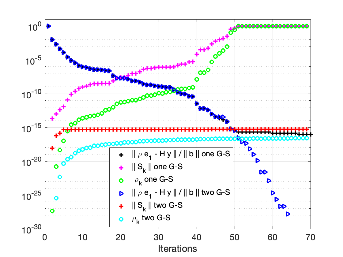
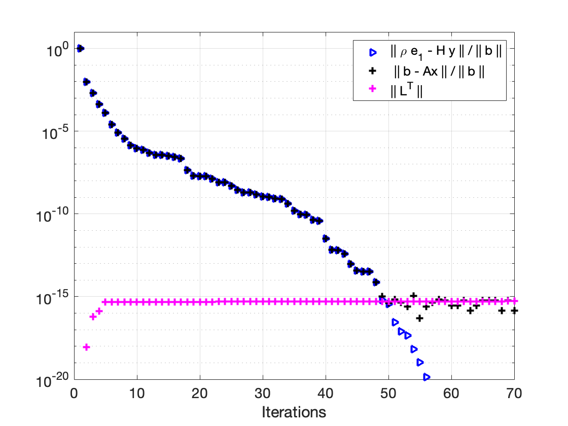
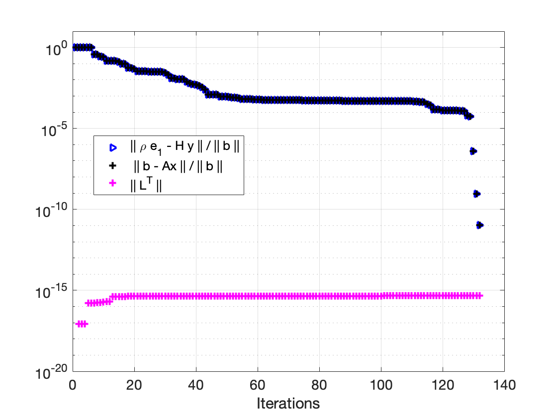
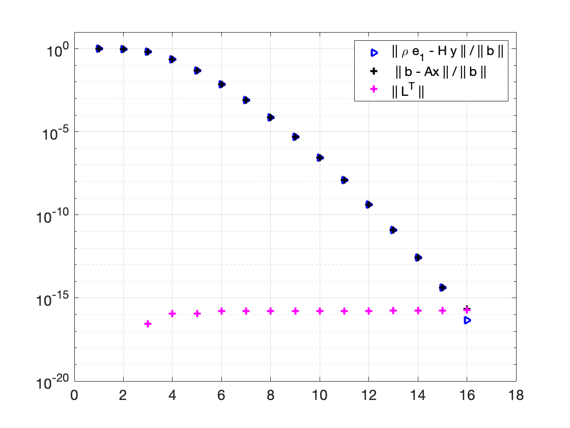
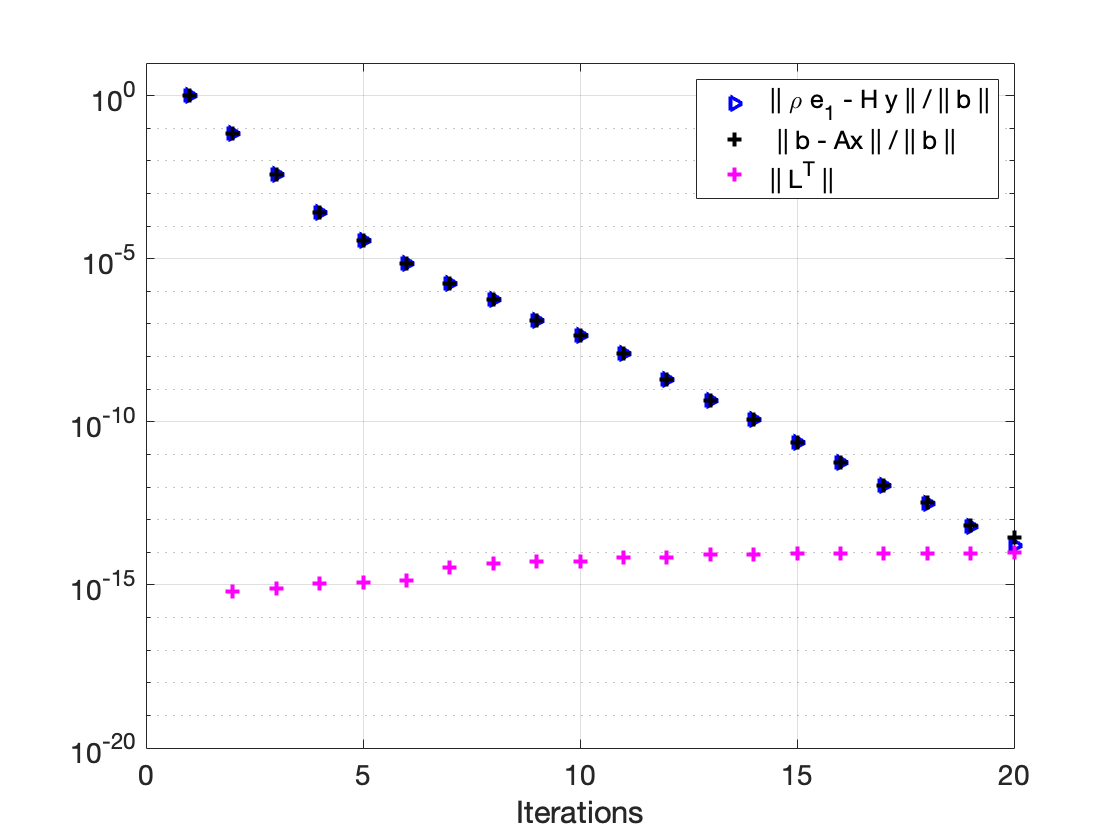
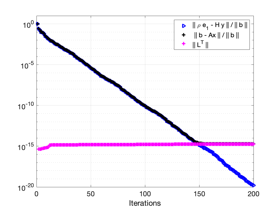
Our first experiment illustrates that the bounds derived in the previous sections properly capture the behavior of the IGS-GMRES algorithm in finite precision. In the next section, we demonstrate that our bounds continue to hold for a broad class of matrices. In particular, we examine the fs1836 matrix studied by Paige and Strakoš [3]. Our Figure 1 should be compared with Figures 7.1 and 7.3 of their (2002) paper. In order to demonstrate empirically that the backward error is reduced by the iteration matrix Mk11Nk1superscriptsubscript𝑀𝑘11subscript𝑁𝑘1M_{k-1}^{-1}N_{k-1}, the quantity Sk(2)2subscriptnormsuperscriptsubscript𝑆𝑘22\|S_{k}^{(2)}\|_{2} is computed, as defined by Paige et al. [2], which measures the loss of orthogonality for two iterations. The spectral radius ρksubscript𝜌𝑘\rho_{k} of the matrix Mk1Nksuperscriptsubscript𝑀𝑘1subscript𝑁𝑘M_{k}^{-1}N_{k} is highly correlated with, and follows the metric, Sk(2)2subscriptnormsuperscriptsubscript𝑆𝑘22\|S_{k}^{(2)}\|_{2}. The metric Sk(2)2subscriptnormsuperscriptsubscript𝑆𝑘22\|S_{k}^{(2)}\|_{2} is plotted for one and two Gauss-Seidel iterations in Figure 1. The Arnoldi relative residuals are plotted as in Figure 7.1 of Paige and Strakoš [3], which, for one iteration, stagnate near iteration forty-three at 1×1071superscript1071\times 10^{-7} before reaching 𝒪(ε)𝒪𝜀{\cal O}(\varepsilon). For two Gauss-Seidel iterations, the (Arnoldi) relative residual continues to decrease monotonically and the norm-wise relative backward error (3) reaches the level of machine precision: β(𝐱k)=6.6×10¹⁷𝛽subscript𝐱𝑘6.6superscript1017\beta(\mathbf{x}_{k})=6.6\times 10^{-17} at iteration fifty. Most notably, the 2-norm of A𝐴A is large, where A2=1.2×10⁹subscriptnorm𝐴21.2superscript109\|A\|_{2}=1.2\times 10^{9}.

Refer to caption
Figure 1: fs1836 matrix. Arnoldi relative residual, spectral radius of Mk1Nksuperscriptsubscript𝑀𝑘1subscript𝑁𝑘M_{k}^{-1}N_{k} and Paige’s Sknormsubscript𝑆𝑘\|S_{k}\| for one and two Gauss-Seidel iterations.

A normal matrix Xn×n𝑋superscript𝑛𝑛X\in\mathbb{C}^{n\times n} satisfies XX=XXsuperscript𝑋𝑋𝑋superscript𝑋X^{*}X=XX^{*}. Henrici’s definition of the departure from normality

(41) dep(X)=XF2Λ(X)F2,dep𝑋superscriptsubscriptnorm𝑋𝐹2superscriptsubscriptnormΛ𝑋𝐹2{\rm dep}(X)=\sqrt{\|X\|_{F}^{2}-\|\Lambda(X)\|_{F}^{2}},

where Λ(X)n×nΛ𝑋superscript𝑛𝑛\Lambda(X)\in\mathbb{C}^{n\times n} is the diagonal matrix containing the eigenvalues of X𝑋X [23], serves as a useful metric for the loss of orthogonality. While we find practical use for this metric for measuring the degree of (non)normality of a matrix, there are of course other useful metrics to describe (non)normality. We refer the reader to [24, 23, 25] and references therein. In particular, the loss of orthogonality is signaled by the departure from normality as follows:

(42) dep2(Mk1)=dep2(I+Lk)=I+LkF2IF2=IF2+LkF2k=LkF2.superscriptdep2superscriptsubscript𝑀𝑘1superscriptdep2𝐼subscript𝐿𝑘superscriptsubscriptnorm𝐼subscript𝐿𝑘𝐹2superscriptsubscriptnorm𝐼𝐹2superscriptsubscriptnorm𝐼𝐹2superscriptsubscriptnormsubscript𝐿𝑘𝐹2𝑘superscriptsubscriptnormsubscript𝐿𝑘𝐹2{\rm dep}^{2}(M_{k}^{-1})={\rm dep}^{2}(I+L_{k})=\|I+L_{k}\|_{F}^{2}-\|I\|_{F}^{2}=\|I\|_{F}^{2}+\|L_{k}\|_{F}^{2}-k=\|L_{k}\|_{F}^{2}.

Note that for the iteration matrix Mk1Nk=(I+Lk)1LkTsubscriptsuperscript𝑀1𝑘subscript𝑁𝑘superscript𝐼subscript𝐿𝑘1superscriptsubscript𝐿𝑘𝑇M^{-1}_{k}N_{k}=(I+L_{k})^{-1}L_{k}^{T} we have, and it is observed in practice, that Mk1Nk2Mk1NkFLkFsubscriptnormsubscriptsuperscript𝑀1𝑘subscript𝑁𝑘2subscriptnormsubscriptsuperscript𝑀1𝑘subscript𝑁𝑘𝐹subscriptnormsubscript𝐿𝑘𝐹\|M^{-1}_{k}N_{k}\|_{2}\leq\|M^{-1}_{k}N_{k}\|_{F}\approx\|L_{k}\|_{F} up to the first order in ε𝜀\varepsilon.

5 Numerical Results

Numerically challenging test problems for GMRES have been proposed and analyzed over the past 35 years. These include both symmetric and non-symmetric matrices. Simoncini and Szyld [26] introduced a symmetric, diagonal matrix with real eigenvalues, causing MGS-GMRES residuals to stagnate. Highly non-normal matrices from Walker [9] were used to explore the convergence characteristics of HH-GMRES and then the non-normal fs1836 from Paige et al. [2] and west0132 from Paige and Strakoš[3] encountering stagnation. In addition to these, we consider the impcol_e matrix from Greenbaum et al. [27]. Matrices with complex eigenvalues forming a disc inside the unit circle such as the Helmert matrix from Liesen and Tichý [28], are also evaluated. Results from a pressure continuity solver with AMG preconditioner and a circuit simulation with the ADD32 matrix from Rozložník, Strakoš, and Tuma [29] are also presented. Numerical results were obtained with Algorithm 4.1 and we verified that Algorithm 4.2 computations are comparable. In particular, the diagonal elements Rk,ksubscript𝑅𝑘𝑘R_{k,k} computed with the lagged norm agree closely with those from Algorithm 4.1. In all cases, the orthogonality between the computed vectors remains on the level 𝒪(ε)𝒪𝜀{\cal O}(\varepsilon), the smallest singular value of V¯ksubscript¯𝑉𝑘\bar{V}_{k} remains close to one, and the Krylov basis vectors remain linearly independent. Therefore the norm of the true relative residual reaches the level 𝒪(ε)𝒪𝜀{\cal O}(\varepsilon) at least by the final iteration, while the Arnoldi residual continues to decrease far below this level.

Ill-Conditioned Diagonal Matrix

Simoncini and Szyld [26] consider several difficult and very ill-conditioned problems that can lead to stagnation of the residual before converging to the level of machine precision 𝒪(ε)𝒪𝜀{\cal O}(\varepsilon). In their example 5.5, they construct A=diag([1e4,2,3,,100])𝐴diag1𝑒423100A={\rm diag}([1e-4,2,3,\ldots,100]), a diagonal matrix, and the right-hand side 𝐛=randn(100,1)𝐛randn1001\mathbf{b}={\rm randn}(100,1) is normalized so that 𝐛2=1subscriptnorm𝐛21\|\mathbf{b}\|_{2}=1. The condition number of this matrix is κ(A)=1×10⁶𝜅𝐴1superscript106\kappa(A)=1\times 10^{6} and A2=100subscriptnorm𝐴2100\|A\|_{2}=100. With the MGS-GMRES algorithm, the relative residual stagnates at the level 1×10121superscript10121\times 10^{-12} after 75 iterations, when Sk2=1subscriptnormsubscript𝑆𝑘21\|S_{k}\|_{2}=1, indicating that the Krylov vectors are not linearly independent. In the case of the iterative Gauss-Seidel formulation of GMRES (with two Gauss-Seidel iterations), the convergence history is plotted in Figure 2, where it can be observed that the relative Arnoldi residual continues to decrease monotonically. Furthermore, the true relative residual is plotted along with Lk1Fsubscriptnormsubscript𝐿𝑘1𝐹\|L_{k-1}\|_{F}. The latter indicates that a significant loss of orthogonality does not occur.

Ill-Conditioned Symmetric and Non-Symmetric Matrices

Figures 1.1 and 1.2 from Greenbaum et al. [27] describe the results for STEAM1 (using the HH and MGS implementations of GMRES, respectively). Similarly, Figures 1.3 and 1.4 from Greenbaum et al. [27] correspond to IMPCOLE. They emphasize that the convergence behavior illustrated in these plots is typical of the MGS-GMRES and HH-GMRES algorithms. The condition number of the system matrix is κ(A)=2.855×10⁷𝜅𝐴2.855superscript107\kappa(A)=2.855\times 10^{7} and A2=2.2×10⁷subscriptnorm𝐴22.2superscript107\|A\|_{2}=2.2\times 10^{7} for STEAM1, whereas κ(A)=7.102×10⁶𝜅𝐴7.102superscript106\kappa(A)=7.102\times 10^{6} and A2=5.0×10³subscriptnorm𝐴25.0superscript103\|A\|_{2}=5.0\times 10^{3} for IMPCOLE.

Greenbaum et al. [27] observe that although orthogonality of the Krylov vectors is not maintained near machine precision, as is the case for the Householder implementation, the relative residuals of the MGS-GMRES algorithm are almost identical to those of the HH-GMRES until the smallest singular value of the matrix V¯ksubscript¯𝑉𝑘\bar{V}_{k} begins to depart from one. At that point the MGS-GMRES relative residual norm begins to stagnate close to its final precision level. This observation is demonstrated with the numerical examples for matrices STEAM1 (N=240𝑁240N=240, symmetric positive definite matrix used in oil recovery simulations) and IMPCOLE (N=225𝑁225N=225, nonsymmetric matrix from modelling of the hydrocarbon separation problem). In both experiments 𝐱=(1,,1)T𝐱superscript11𝑇\mathbf{x}=(1,...,1)^{T}, 𝐛=A𝐱𝐛𝐴𝐱\mathbf{b}=A\mathbf{x} and 𝐱0=𝟎subscript𝐱00\mathbf{x}_{0}={\bf 0}. The convergence histories for the iterated Gauss-Seidel GMRES algorithm applied to these matrices are plotted in Figures 3 and 4. A significant loss of orthogonality is not observed until the last iteration. Otherwise the computed metric Lk1Fsubscriptnormsubscript𝐿𝑘1𝐹\|L_{k-1}\|_{F} and the true relative residual remain near 𝒪(ε)𝒪𝜀{\cal O}(\varepsilon). The Arnoldi residual continues to decrease and the smallest singular value of Vksubscript𝑉𝑘V_{k} is 0.999850.999850.99985.

Highly Non-Normal Matrices

Bidiagonal matrices with a δ𝛿\delta off-diagonal were studied by Embree [30]. These are non-normal matrices where 0<δ10𝛿10<\delta\leq 1 and are completely defective for all δ0𝛿0\delta\neq 0. A defective matrix is a square matrix that does not have a complete basis of eigenvectors, and is therefore not diagonalizable, and the pseudo-spectra [25] of these matrices are discs in the complex plane. Our IGS-GMRES algorithm leads to convergence after 16 iterations without stagnation and orthogonality is maintained to machine precision as plotted in Figure 5. The matrix 2-norm is A2=1.1subscriptnorm𝐴21.1\|A\|_{2}=1.1 and condition κ(A)=1.2𝜅𝐴1.2\kappa(A)=1.2. Walker [9] employed the highly non-normal matrix in equation (43) to compare the Gram-Schmidt and Householder implementations of GMRES. The element α𝛼\alpha controls both the condition number κ(A)𝜅𝐴\kappa(A) and the departure from normality dep(A)dep𝐴{\rm dep}(A) of the matrix of size n×n𝑛𝑛n\times n. Here A2=2.0×10³subscriptnorm𝐴22.0superscript103\|A\|_{2}=2.0\times 10^{3}.

(43) A=[100α0200000n],𝐛=[111]formulae-sequence𝐴delimited-[]100𝛼0200missing-subexpression000𝑛𝐛delimited-[]111A=\left[\begin{array}[]{ccccc}1&0&\cdots&0&\alpha\\ 0&2&\cdots&0&0\\ \vdots&\vdots&&\vdots&\vdots\\ 0&0&\cdots&0&n\end{array}\right],\quad\mathbf{b}=\left[\begin{array}[]{c}1\\ 1\\ \vdots\\ 1\end{array}\right]

For large values of α𝛼\alpha, Walker found that the MGS residual would stagnate and that the CGS algorithm led to instability. Furthermore, it was found that even CGS-2 with re-orthogonalization exhibited some instability near convergence. HH-GMRES maintains 𝒪(ε)𝒪𝜀{\cal O}(\varepsilon) orthogonality as measured by IV¯kTV¯kFsubscriptnorm𝐼superscriptsubscript¯𝑉𝑘𝑇subscript¯𝑉𝑘𝐹\|I-\bar{V}_{k}^{T}\bar{V}_{k}\|_{F} and reduces the relative residual to machine precision.

In our experiments, the value α=2000𝛼2000\alpha=2000 leads to a matrix with κ(A)=4×10⁵𝜅𝐴4superscript105\kappa(A)=4\times 10^{5}. The departure from normality, based on Henrici’s metric, is large: dep(A)=2000dep𝐴2000{\rm dep}(A)=2000. The convergence history is displayed in Figure 6. The loss of orthogonality remains near O(ε)𝑂𝜀O(\varepsilon) and our upper bound is close for this problem. Notably, the oscillations present in the relative residual computed by the CGS-2 variant are not present in the iterated Gauss-Seidel convergence history plots, where the Arnoldi relative residual decreases monotonically.

Paige and Strakoš [3] experimented with MGS-GMRES convergence for the non-normal matrices FS1836 and WEST0132. In all their experiments 𝐛=(1,,1)T𝐛superscript11𝑇\mathbf{b}=(1,\ldots,1)^{T} . The matrix FS1836 has dimension n=183𝑛183n=183, with A21.2×109subscriptnorm𝐴21.2superscript109\|A\|_{2}\approx 1.2\times 10^{9}, and κ(A)1.5×10¹¹𝜅𝐴1.5superscript1011\kappa(A)\approx 1.5\times 10^{11}. The matrix WEST0132 has n=132𝑛132n=132, A23.2×105subscriptnorm𝐴23.2superscript105\|A\|_{2}\approx 3.2\times 10^{5}, and κ(A)6.4×10¹¹𝜅𝐴6.4superscript1011\kappa(A)\approx 6.4\times 10^{11}. Their Figure 7.1 indicates that the relative residual for FS1836 stagnates at 1×1071superscript1071\times 10^{-7} at iteration 43 when orthogonality is lost. The relative residual for the WEST0132 matrix also stagnates at the 1×1071superscript1071\times 10^{-7} level after 130 iterations. These results contrast with our Figures 7 and 8. In both cases the Arnoldi residuals continue to decrease and Lk1Fsubscriptnormsubscript𝐿𝑘1𝐹\|L_{k-1}\|_{F} grows slowly or remains close to machine precision. The smallest singular value remains at σmin(V¯k)=1subscript𝜎subscript¯𝑉𝑘1\sigma_{\min}(\bar{V}_{k})=1 for both matrices.

Complex Eigenvalues in a Disc

Liesen and Tichý [28] employ the Helmert matrix generated by the MATLAB command gallery(’orthog’,18,4). Helmert matrices occur in a number of practical problems, for example in applied statistics. The matrix is orthogonal, and the eigenvalues cluster around 11-1, as in the right panels of their Figure 4.4. The worst-case MGS-GMRES residual norm decreases quickly throughout the iterations and stagnates at the 12–th iteration, where the relative residual remains at 1×10101superscript10101\times 10^{-10}. From the convergence history plotted in Figure 9, the loss of orthogonality remains near machine precision and the Arnoldi relative residual does not stagnate. The quantity Lk1Fsubscriptnormsubscript𝐿𝑘1𝐹\|L_{k-1}\|_{F} is an excellent predictor of the orthogonality.

Nalu-Wind Model

Nalu-Wind solves the incompressible Navier-Stokes equations, with a pressure projection. The governing equations are discretized in time with a BDF-2 integrator, where an outer Picard fixed-point iteration is employed to reduce the nonlinear system residual at each time step. Within each time step, the Nalu-Wind simulation time is often dominated by the time required to setup and solve the linearized governing equations. The pressure systems are solved using GMRES with an AMG preconditioner, where a polynomial Gauss-Seidel smoother is now applied are described in Mullowney et al. [31]. Hence, relaxation is a compute time intensive component, when employed as a smoother.

The McAlister experiment for wind-turbine blades is an unsteady RANS simulation of a fixed-wing, with a NACA0015 cross section, operating in uniform inflow. Resolving the high-Reynolds number boundary layer over the wing surface requires resolutions of 𝒪(105)𝒪superscript105{\cal O}(10^{-5}) normal to the surface resulting in grid cell aspect ratios of 𝒪(40,000)𝒪40000{\cal O}(40,000). These high aspect ratios present a significant challenge. The simulations were performed for the wing at 12 degree angle of attack, 1 m chord length, denoted c𝑐c, aspect ratio of 3.3, i.e., s=3.3c𝑠3.3𝑐s=3.3c, and square wing tip. The inflow velocity is u=46subscript𝑢46u_{\infty}=46 m/s, the density is ρ=1.225subscript𝜌1.225\rho_{\infty}=1.225 kg/m3kgsuperscriptm3{\rm kg/m}^{3}, and dynamic viscosity is μ=3.756×10⁵𝜇3.756superscript105\mu=3.756\times 10^{-5} kg/(m s), leading to a Reynolds number Re=1.5×10⁶𝑅𝑒1.5superscript106Re=1.5\times 10^{6}. Due to the complexity of mesh generation, only one mesh with approximately 3 million grid points was generated.

The smoother is hybrid block-Jacobi with two sweeps of polynomial Gauss-Seidel relaxation applied locally on a subdomain and then Jacobi smoothing for globally shared degrees of freedom. The coarsening rate for the wing simulation is roughly 4×4\times with eight levels in the V𝑉V-cycle for hypre [32]. Operator complexity C𝐶C is approximately 1.61.61.6 indicating more efficient V𝑉V-cycles with aggressive coarsening, however, an increased number of solver iterations are required compared to standard coarsening. The convergence history is plotted in Figure 10, where the loss of orthogonality is completely flat and close to machine precision.

Circuit Simulation

Rozložník et al. [29] study a typical linear system arising in circuit simulation (the matrix from a 32-bit adder design). The matrix has A2=0.05subscriptnorm𝐴20.05\|A\|_{2}=0.05 and κ(A)=213𝜅𝐴213\kappa(A)=213. In exact arithmetic the Arnoldi vectors are orthogonal. However, in finite precision computation the orthogonality is lost, which may potentially affect approximate solution. In their Figure 3, the authors have plotted the loss of orthogonality of the computed Krylov vectors for different implementations of the GMRES method (MGS, Householder and CGS). The comparable results for IGS-GMRES are plotted in Figure 11. The smallest singular value remains at σmin(V¯k)=1subscript𝜎subscript¯𝑉𝑘1\sigma_{\min}(\bar{V}_{k})=1.

6 Conclusions

The essential contribution of our work was to derive an iterative Gauss-Seidel formulation of the GMRES algorithm due to Saad and Schultz [1] that employs approximate solutions of the normal equations appearing in the Gram-Schmidt projector, based on observations of Ruhe [6] and the low-synchronization algorithms introduced by Świrydowicz et al.  [4].

The insights gained from the seminal work of Ruhe [6] led us to the conclusion that the modified Gram-Schmidt algorithm is equivalent to one step of a multiplicative Gauss-Seidel iteration method applied to the normal equations Qk1TQk1𝐫1:k1,k=Qk1T𝐚ksuperscriptsubscript𝑄𝑘1𝑇subscript𝑄𝑘1subscript𝐫:1𝑘1𝑘superscriptsubscript𝑄𝑘1𝑇subscript𝐚𝑘Q_{k-1}^{T}Q_{k-1}\>\mathbf{r}_{1:k-1,k}=Q_{k-1}^{T}\mathbf{a}_{k}. Similarly, the classical Gram-Schmidt algorithm can be viewed as one step of an additive Jacobi relaxation. The projector is then given by P𝐚k=𝐚kQk1Tk1Qk1T𝐚k𝑃subscript𝐚𝑘subscript𝐚𝑘subscript𝑄𝑘1subscript𝑇𝑘1superscriptsubscript𝑄𝑘1𝑇subscript𝐚𝑘P\mathbf{a}_{k}=\mathbf{a}_{k}-Q_{k-1}\>T_{k-1}\>Q_{k-1}^{T}\mathbf{a}_{k}, where Tk1subscript𝑇𝑘1T_{k-1} is a correction matrix. In the case of DCGS-2, with delayed re-orthogonalization, Bielich et al. [5] split and apply the symmetric (normal) correction matrix across two Arnoldi iterations and then apply Stephen’s trick to maintain orthogonality. For MGS, the lower triangular matrix Tk1(Qk1TQk1)1subscript𝑇𝑘1superscriptsuperscriptsubscript𝑄𝑘1𝑇subscript𝑄𝑘11T_{k-1}\approx(\>Q_{k-1}^{T}Q_{k-1}\>)^{-1} appearing in Świrydowicz et al. [4] was identified as the inverse compact WY𝑊𝑌WY form with Tk1(1)=(I+Lk1)1subscriptsuperscript𝑇1𝑘1superscript𝐼subscript𝐿𝑘11T^{(1)}_{k-1}=(I+L_{k-1})^{-1}, where the strictly lower triangular matrix Lk1subscript𝐿𝑘1L_{k-1} was computed from the loss of orthogonality relation

Qk1TQk1=I+Lk1+Lk1T.superscriptsubscript𝑄𝑘1𝑇subscript𝑄𝑘1𝐼subscript𝐿𝑘1superscriptsubscript𝐿𝑘1𝑇Q_{k-1}^{T}Q_{k-1}=I+L_{k-1}+L_{k-1}^{T}.

The matrix Tk1subscript𝑇𝑘1T_{k-1} from the inverse compact WY𝑊𝑌WY form of the Gram-Schmidt projector was also present, without having been explicitly defined, in the rounding error analysis of Björck [13], in Lemma 5.1. In effect, the low-synchronization Gram-Schmidt algorithm presented in [4] represents one iteration step, with a zero initial guess, to construct an approximate projector. When two iteration steps are applied, the resulting correction matrix Tk1(2)superscriptsubscript𝑇𝑘12T_{k-1}^{(2)} is close to a symmetric (normal) matrix:

Tk1(2)=Mk11[I+Nk1Mk11]=Tk1(1)Tk1(1)Lk1TTk1(1).superscriptsubscript𝑇𝑘12superscriptsubscript𝑀𝑘11delimited-[]𝐼subscript𝑁𝑘1superscriptsubscript𝑀𝑘11superscriptsubscript𝑇𝑘11superscriptsubscript𝑇𝑘11superscriptsubscript𝐿𝑘1𝑇superscriptsubscript𝑇𝑘11T_{k-1}^{(2)}=M_{k-1}^{-1}\>[\>I+N_{k-1}\>M_{k-1}^{-1}\>]=T_{k-1}^{(1)}-T_{k-1}^{(1)}\>L_{k-1}^{T}\>T_{k-1}^{(1)}.

However, the Gauss-Seidel formulation described by Ruhe [6] differs from MGS-2 in floating-point arithmetic and the incremental MGS-2 iterative refinement steps allow us to prove backward stability. When employed to compute the Arnoldi-QR𝑄𝑅QR expansion, the GMRES formulation with two Gauss Seidel iterations results in an 𝒪(ε)𝒪𝜀{\cal O}(\varepsilon) backward error, preserving the orthogonality of the Krylov basis vectors to the level 𝒪(ε)𝒪𝜀{\cal O}(\varepsilon), which is measured by Lk1Fsubscriptnormsubscript𝐿𝑘1𝐹\|L_{k-1}\|_{F}. This result is related to recent work on the iterative solution of triangular linear systems using Jacobi iterations that may diverge for highly non-normal triangular matrices [33].

Here, the departure from normality of the inverse of the correction matrix Tk1(1)subscriptsuperscript𝑇1𝑘1T^{(1)}_{k-1} is a measure of the loss of orthogonality. In this formulation, the matrix is lower triangular and can substantially depart from normality as signaled by σmax2(I+Lk1)>1subscriptsuperscript𝜎2𝐼subscript𝐿𝑘11\sigma^{2}_{\max}(I+L_{k-1})>1. Because the correction matrix Tk1(2)subscriptsuperscript𝑇2𝑘1T^{(2)}_{k-1} associated with two iterations of Gauss–Seidel is close to a symmetric (normal) matrix, the singular values of the inverse remain close to one. A departure from normality indicates a possible loss of numerical rank for the Krylov basis vectors Vksubscript𝑉𝑘V_{k} with the smallest singular value decreasing from one. Our numerical experiments, on challenging problems proposed over the past thirty-five years, demonstrate the robust convergence and low relative error achievable with our IGS-GMRES. Furthermore, with one iteration step the loss of orthogonality is at most 𝒪(ε)κ(Bk)𝒪𝜀𝜅subscript𝐵𝑘{\cal O}(\varepsilon)\kappa(B_{k}) and for the algorithm with two iterations, it remains near machine precision.

We have demonstrated that the iterated Gauss Seidel GMRES with two iterations is backward stable and does not exhibit stagnation in the Arnoldi residual as defined by Greenbaum et al. [27]. This refers to the approximate residual norm computed as ρ𝐞1Hk+1,k𝐲k2/ρsubscriptnorm𝜌subscript𝐞1subscript𝐻𝑘1𝑘subscript𝐲𝑘2𝜌\|\rho\>\mathbf{e}_{1}-H_{k+1,k}\mathbf{y}_{k}\>\|_{2}/\rho, where 𝐱k=𝐱0+Vk𝐲ksubscript𝐱𝑘subscript𝐱0subscript𝑉𝑘subscript𝐲𝑘\mathbf{x}_{k}=\mathbf{x}_{0}+V_{k}\mathbf{y}_{k} is the approximate solution and the true residual is given by 𝐛A𝐱k𝐛𝐴subscript𝐱𝑘\mathbf{b}-A\mathbf{x}_{k}. The Arnoldi residual does not stagnate and will continue to decrease monotonically. In particular, the true relative residual will decrease towards machine precision level and as noted by Paige et al. [2], the norm-wise relative backward error β(𝐱k)𝛽subscript𝐱𝑘\beta(\mathbf{x}_{k}) will be 𝒪(ε)𝒪𝜀{\cal O}(\varepsilon). In the original algorithm, the Arnoldi residual can stagnate when the Krylov vectors lose linear independence and the smallest singular value of Vksubscript𝑉𝑘V_{k} decreases towards zero. For the iterative Gauss-Seidel GMRES algorithm described herein, the singular values remain close to one and β(𝐱k)𝛽subscript𝐱𝑘\beta(\mathbf{x}_{k}) remains close to machine precision at convergence.

We have also presented a one-reduce algorithm which can be interpreted as an MGS-CGS hybrid. This algorithm merits further study. Algorithm 2 is equivalent to the MGS-CGS GMRES when Lk2=0subscript𝐿𝑘20L_{k-2}=0 at step k1𝑘1k-1 in exact arithmetic and produces similar results in finite precision (in terms of the loss of orthogonality and Arnoldi residual). Our numerical experiments demonstrated that the computed results are comparable to the two-reduce IGS-GMRES and diagonal elements Rk,ksubscript𝑅𝑘𝑘R_{k,k} agree closely when the lagged norm is employed. In particular, the loss of orthogonality remains at 𝒪(ε)𝒪𝜀{\cal O}(\varepsilon) in all of the examples, implying backward stability according to Drkošová et al. [8].

We anticipate that the iterated Gauss-Seidel algorithms will facilitate the construction of backward stable iterative solvers based on block Gram-Schmidt algorithms including enlarged Krylov subspace methods and s𝑠s-step methods. Mixed-precision formulations may also benefit. Randomization and sketching may be applied to the normal equations in the projector, with an oblique inner-product 𝐱TBTB𝐱superscript𝐱𝑇superscript𝐵𝑇𝐵𝐱\mathbf{x}^{T}B^{T}B\mathbf{x} and sketching matrix A𝐴A, leading to even greater computational efficiency. In addition, these developments could be relevant for Anderson acceleration of nonlinear fixed-point iterations, which is currently being applied to optimization algorithms in deep learning for artificial intelligence. The algorithms may also be useful for computing eigenvalues with the Krylov-Schur algorithm of Stewart [21], where 𝒪(ε)𝒪𝜀{\cal O}(\varepsilon) orthogonality is required to obtain an invariant subspace of maximal dimension. We plan to explore the parallel strong-scaling performance of the IGS-GMRES and hybrid MGS-CGS GMRES for large-scale scientific computation on exascale supercomputers.

Acknowledgement

This research was supported by the Exascale Computing Project (17-SC-20-SC), a collaborative effort of the U.S. Department of Energy Office of Science and the National Nuclear Security Administration. The second author was additionally supported by Charles University PRIMUS project no. PRIMUS/19/SCI/11 and Charles University Research program no. UNCE/SCI/023. In addition, ERC Starting Grant No. 101075632. The third author was supported by the Academy of Sciences of the Czech Republic (RVO 67985840) and by the Grant Agency of the Czech Republic, Grant No. 23-06159S. Our work was inspired by the contributions of A. Björck, A. Ruhe, C. C. Paige, Z. Strakoš, and the legacy of Y. Saad and M. H. Schultz that is MGS-GMRES. We also wish to thank our friends and colleagues Julien Langou and Luc Giraud for their thoughtful insights over many years. A sincere thank-you to the organizers of the Copper Mountain conferences on Krylov and multigrid methods for their rich 38+ year tradition of innovative numerical linear algebra. We would also like to thank the two anonymous reviewers for their careful reading of the manuscript. Their thoughtful comments resulted in a much improved presentation.
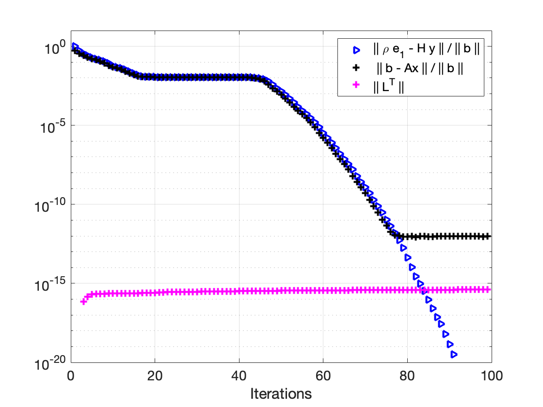
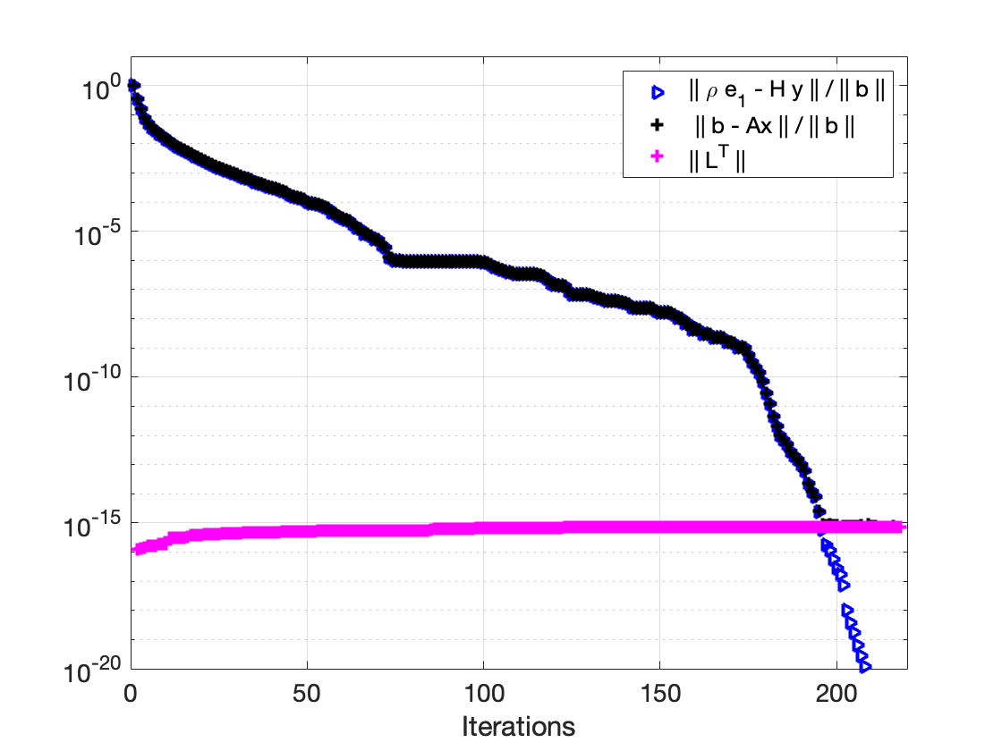
Refer to caption
Figure 2: Simoncini matrix. Arnoldi relative residual. Loss of orthogonality relation (42).
Refer to caption
Figure 3: steam1 matrix. Arnoldi relative residual. Loss of orthogonality relation (42).
Refer to caption
Figure 4: impcol_e matrix. Arnoldi relative residual. Loss of orthogonality relation (42).
Refer to caption
Figure 5: Embree δ𝛿\delta matrix. Arnoldi relative residual. Loss of orthogonality relation (42).
Refer to caption
Figure 6: Walker matrix. Arnoldi relative residual. Loss of orthogonality relation (42).
Refer to caption
Figure 7: fs1863 matrix. Arnoldi relative residual. Loss of orthogonality relation (42).
Refer to caption
Figure 8: west0132 matrix. Arnoldi relative residual. Loss of orthogonality relation (42).
Refer to caption
Figure 9: Helmert matrix. Arnoldi relative residual. Loss of orthogonality relation (42).
Refer to caption
Figure 10: Pressure matrix. Arnoldi relative residual. Loss of orthogonality relation (42).
Refer to caption
Figure 11: Add32 matrix. Arnoldi relative residual. Loss of orthogonality relation (42).

References

  • [1] Y. Saad, M. H. Schultz, GMRES: A generalized minimal residual algorithm for solving nonsymmetric linear systems, SIAM Journal on scientific and statistical computing 7 (3) (1986) 856–869.
  • [2] C. C. Paige, M. Rozložník, Z. Strakoš, Modified Gram-Schmidt (MGS), least squares, and backward stability of MGS-GMRES, SIAM Journal on Matrix Analysis and Applications 28 (1) (2006) 264–284.
  • [3] C. C. Paige, Z. Strakoš, Residual and backward error bounds in minimum residual Krylov subspace methods, SIAM Journal on Scientific and Statistical Computing 23 (6) (2002) 1899–1924.
  • [4] K. Świrydowicz, J. Langou, S. Ananthan, U. Yang, S. Thomas, Low synchronization Gram-Schmidt and generalized minimal residual algorithms, Numerical Linear Algebra with Applications 28 (2020) 1–20.
  • [5] D. Bielich, J. Langou, S. Thomas, K. Świrydowicz, I. Yamazaki, E. Boman, Low-synch Gram-Schmidt with delayed reorthogonalization for Krylov solvers, Parallel Computing (2021).
  • [6] A. Ruhe, Numerical aspects of Gram-Schmidt orthogonalization of vectors, Linear Algebra and its Applications 52 (1983) 591–601.
  • [7] Å. Björck, Numerics of Gram-Schmidt orthogonalization, Linear Algebra and Its Applications 197 (1994) 297–316.
  • [8] J. Drkošová, A. Greenbaum, M. Rozložník, Z. Strakoš, Numerical stability of GMRES, BIT Numerical Mathematics 35 (1995) 309–330.
  • [9] H. F. Walker, Implementation of the GMRES method using Householder transformations, SIAM Journal on Scientific and Statistical Computing 9 (1) (1988) 152–163.
  • [10] L. Giraud, S. Gratton, J. Langou, A rank-k𝑘k update procedure for reorthogonalizing the orthogonal factor from modified Gram-Schmidt, SIAM J. Matrix Analysis and Applications 25 (4) (2004) 1163–1177.
  • [11] Å. Björck, C. C. Paige, Loss and recapture of orthogonality in the modified Gram-Schmidt algorithm, SIAM Journal on Matrix Analysis and Applications 13 (1992) 176–190.
  • [12] S. Lockhart, D. J. Gardner, C. S. Woodward, S. Thomas, L. N. Olson, Performance of low synchronization orthogonalization methods in Anderson accelerated fixed point solvers, in: Proceedings of the 2022 SIAM Conference on Parallel Processing for Scientific Computing (PP), 2022, pp. 49–59.
  • [13] A. Björck, Solving least squares problems by Gram–Schmidt orthogonalization, BIT 7 (1967) 1–21.
  • [14] L. Giraud, J. Langou, M. Rozložník, J. v. d. Eshof, Rounding error analysis of the classical Gram-Schmidt orthogonalization process, Numerische Mathematik 101 (2005) 87–100.
  • [15] N. J. Higham, The accuracy of solutions to triangular systems, SIAM J. Numer. Anal. 26 (5) (1989) 1252–1265.
  • [16] N. J. Higham, Accuracy and Stability of Numerical Algorithms, 2nd Edition, SIAM, 2002.
  • [17] Q. Zou, GMRES algorithms over 35 years (2021). arXiv:2110.04017.
  • [18] I. Yamazaki, S. Thomas, M. Hoemmen, E. G. Boman, K. Świrydowicz, J. J. Elliott, Low-synchronization orthogonalization schemes for s𝑠s-step and pipelined Krylov solvers in Trilinos, in: SIAM 2020 Conference on Parallel Processing for Scientific Computing, SIAM, 2020, pp. 118–128.
  • [19] E. Carson, K. Lund, M. Rozložník, S. Thomas, Block Gram-Schmidt algorithms and their stability properties, Linear Algebra and its Applications 638 (2022) 150–195.
  • [20] E. Carson, K. Lund, M. Rozložník, The stability of block variants of classical Gram–Schmidt, SIAM Journal on Matrix Analysis and Applications 42 (3) (2021) 1365–1380.
  • [21] G. W. Stewart, A Krylov–Schur algorithm for large eigenproblems, SIAM Journal on Matrix Analysis and Applications 23 (3) (2001) 601–614.
  • [22] A. Bienz, W. Gropp, L. Olson, Node-aware improvements to allreduce, in: Proceedings of the 2019 IEEE/ACM Workshop on Exascale MPI (ExaMPI), Association for Computing Machinery, 2019, pp. 1–10.
  • [23] P. Henrici, Bounds for iterates, inverses, spectral variation and fields of values of non-normal matrices, Numerische Mathematik 4 (1) (1962) 24–40.
  • [24] I. C. Ipsen, A note on the field of values of non-normal matrices, Tech. rep., North Carolina State University. Center for Research in Scientific Computation (1998).
  • [25] L. Trefethen, M. Embree, The behavior of nonnormal matrices and operators, Spectra and Pseudospectra (2005).
  • [26] V. Simoncini, D. B. Szyld, Theory of inexact krylov subspace methods and applications to scientific computing, SIAM Journal on Scientific Computing 25 (2) (2003) 454–477.
  • [27] A. Greenbaum, M. Rozložník, Z. Strakoš, Numerical behaviour of the modified Gram-Schmidt GMRES implementation, BIT 37 (3) (1997) 706–719.
  • [28] J. Liesen, P. Tichý, The worst-case GMRES for normal matrices, BIT Numer Math 44 (2004) 79–98.
  • [29] M. Rozložník, Z. Strakoš, M. Tuma, On the role of orthogonality in the GMRES method, in: K. G. Jeffery, J. Král, M. Bartosek (Eds.), SOFSEM ’96: Theory and Practice of Informatics, Proceedings, Vol. 1175 of Lecture Notes in Computer Science, Springer, 1996, pp. 409–416.
  • [30] M. Embree, How descriptive are GMRES convergence bounds?, Tech. Rep. Tech. Rep. 99/08, Mathematical Institute, University of Oxford, UK (1999).
  • [31] P. Mullowney, R. Li, S. Thomas, S. Ananthan, A. Sharma, A. Williams, J. Rood, M. A. Sprague, Preparing an incompressible-flow fluid dynamics code for exascale-class wind energy simulations, in: Proceedings of the ACM/IEEE Supercomputing 2021 Conference, ACM, 2021, pp. 1–11.
  • [32] R. D. Falgout, J. E. Jones, U. M. Yang, The design and implementation of hypre, a library of parallel high performance preconditioners, in: A. M. Bruaset, A. Tveito (Eds.), Numerical Solution of Partial Differential Equations on Parallel Computers, Springer Berlin Heidelberg, Berlin, Heidelberg, 2006, pp. 267–294.
  • [33] E. Chow, H. Anzt, J. Scott, J. Dongarra, Using jacobi iterations and blocking for solving sparse triangular systems in incomplete factorization preconditioning, Journal of Parallel and Distributed Computing 119 (2018) 219–230.