4DAC: Learning Attribute Compression for Dynamic Point Clouds

Abstract.

With the development of the 3D data acquisition facilities, the increasing scale of acquired 3D point clouds poses a challenge to the existing data compression techniques. Although promising performance has been achieved in static point cloud compression, it remains under-explored and challenging to leverage temporal correlations within a point cloud sequence for effective dynamic point cloud compression. In this paper, we study the attribute (e.g., color) compression of dynamic point clouds and present a learning-based framework, termed 4DAC. To reduce temporal redundancy within data, we first build the 3D motion estimation and motion compensation modules with deep neural networks. Then, the attribute residuals produced by the motion compensation component are encoded by the region adaptive hierarchical transform into residual coefficients. In addition, we also propose a deep conditional entropy model to estimate the probability distribution of the transformed coefficients, by incorporating temporal context from consecutive point clouds and the motion estimation/compensation modules. Finally, the data stream is losslessly entropy coded with the predicted distribution. Extensive experiments on several public datasets demonstrate the superior compression performance of the proposed approach.

1. Introduction

Figure 1. Point cloud attribute compression results on the sequence “Phil” of the MVUB (Loop et al., 2016) dataset. The state-of-the-art learning-based static attribute compression method, 3DAC (Fang et al., 2022), is presented with our proposed 4DAC. Bits Per Point (BPP) and Peak Signal-to-Noise Ratio (PSNR) of the luminance component are also reported. Note that, raw RGB data of point cloud is usually stored as uint8 (i.e., $8\times 3=24$ BPP).

As a common 3D representation, point cloud has been widely used in several real-world applications such as mixed reality (Pan et al., 2006) and autonomous driving (Geiger et al., 2012; Hu et al., 2021b) due to its compactness and simplicity. With the evolution of 3D laser scanning techniques and depth sensors, dynamic point clouds, which are composed of a sequence of static point clouds, have attracted increasing attention in recent years. Nevertheless, it remains a critical and challenging issue for the community on how to effectively compress unstructured point cloud streams. A handful of recent works, including MPEG standard (Schwarz et al., 2018), and several learning-based approaches in literature (Huang et al., 2020; Biswas et al., 2020; Que et al., 2021; Huang and Liu, 2019; Yan et al., 2019; Quach et al., 2019, 2020; Gao et al., 2021; Wang et al., 2021) have shown encouraging performance on point cloud geometry compression (e.g., the 3D coordinates of points). However, the corresponding point cloud attributes (e.g., remission, color) have been largely overlooked by the community. Moreover, these attributes also take up a large amount of the overall bitstream in practice. Motivated by this, we mainly focus on attribute compression of dynamic point clouds in this paper.

Early works (Mekuria et al., 2016; De Queiroz and Chou, 2017; Dorea and de Queiroz, 2018; Dorea et al., 2019) on dynamic point cloud attribute compression simply follow the common practice of video compression. Specifically, these methods usually follow a three-step pipeline, including 3D motion estimation and compensation, transform coding, and entropy coding. In particular, 3D motion estimation is the key component to reduce temporal redundancy within consecutive point clouds. Although encouraging effects has been achieved, the overall compression ratio is still limited by the hand-crafted motion estimation modules. Furthermore, other modules of the compression framework, such as entropy coding, are designed and optimized independently without considering the valuable temporal information.

Recently, a number of deep learning-based algorithms (Alexiou et al., 2020; Sheng et al., 2021; Isik et al., 2021) are proposed for compressing point cloud attributes. In general, these methods build the transform coding or entropy coding module with the powerful deep neural networks, hence are likely to achieve comparable or even better performance than traditional hand-crafted compression algorithms. However, these methods mainly focus on the compression of static point clouds and do not consider the temporal correlations in consecutive point clouds. MuSCLE (Biswas et al., 2020) is the only learning-based algorithm proposed to compress the intensity of LiDAR point cloud streams. Nevertheless, the compression performance is still limited by its naive framework, which does not have any motion estimation or transform coding blocks, and there is only spatial-temporal aggregation to extract temporal context for its entropy model.

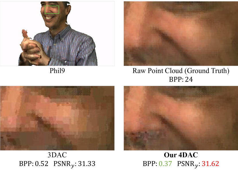
In this paper, we present a learning-based attribute compression framework, termed 4DAC, for dynamic point clouds. Specifically, we propose two separate networks for 3D motion estimation and motion compensation. Region Adaptive Hierarchical Transform (RAHT) is adopted to encode the temporal attribute residuals produced by motion compensation to frequency-domain coefficients. Then, we further exploit temporal contexts to construct a deep conditional entropy model to estimate the probability distribution of the transformed coefficients. In particular, explicit and implicit temporal correlations hidden in consecutive point clouds and motion estimation/compensation blocks are explored for probability estimation. Finally, we feed the coefficients and their predicted distribution to an arithmetic coder to further compress the data stream losslessly. As shown in Fig. 1, by leveraging the useful temporal information, our method achieves better quantitative and qualitative compression performance than the static point cloud compression counterpart, 3DAC (Fang et al., 2022). Our key contributions are as follows:

• We propose an effective learning-based framework for dynamic point cloud compression, which is composed of a deep 3D motion estimation block, a deep 3D compensation block, and a deep entropy model.

• We propose a temporal conditional entropy model to explore both explicit and implicit temporal correlation within data and motion estimation/compensation blocks.

• Extensive experiments demonstrate the state-of-the-art compression performance achieved by our 4DAC on several point cloud benchmarks.

2. Related Work

2.1. Point Cloud Geometry Compression

Point cloud geometry compression focuses on compressing the 3D coordinates of each point. Part of works (Meagher, 1982; Schwarz et al., 2018; Kammerl et al., 2012; Garcia et al., 2019) rely on the octree structure to compress point cloud geometry. These works usually organize raw point cloud data as an octree and further entropy code the octants to a compact bitstream. To exploit temporal information within point cloud sequences, Kammerl et al. (Kammerl et al., 2012) differentially encoded subsequent octree as XOR differences and Garcia et al. (Garcia et al., 2019) introduced temporal context for entorpy coding. Recently, some learning-based compression methods (Huang et al., 2020; Biswas et al., 2020; Que et al., 2021; Fu et al., 2022) also adopt the octree strcuture and construct their octree-based entropy models to reduce data redundancy. Inspired by deep image compression (Ballé et al., 2018), other learning-based approaches (Huang and Liu, 2019; Yan et al., 2019; Quach et al., 2019, 2020; Gao et al., 2021; Wang et al., 2021) adopt 3D auto-encoders (Qi et al., 2017a; Brock et al., 2016; Choy et al., 2019) to achieve point cloud geometry compression. However, most of these methods are geometry-oriented and it is still a non-trivial task to extend them to attribute compression of dynamic point clouds.

2.2. Point Cloud Attribute Compression

Point cloud attribute compression aims at compressing the attributes (e.g., color) of points. Attribute compression algorithms can be roughly categorized as static or dynamic compression.

Static attribute compression methods (Zhang et al., 2014; Shao et al., 2017, 2018; De Queiroz and Chou, 2016; Souto and de Queiroz, 2020; Pavez et al., 2021, 2020; Schwarz et al., 2018; Gu et al., 2019) usually include two steps, transform coding of attributes, which captures data spatial redundancy in the transformed domain, and entropy coding of transformed coefficients, which losslessly compresses symbols into a compact bitstream. For example, Zhang et al. (Zhang et al., 2014) encoded the voxliezed point cloud through graph transform and then entropy coded the transformed coefficients with a Laplacian probability distribution. Queiroz et al. (De Queiroz and Chou, 2016) proposed a 3D Haar wavelet transform, namely RAHT, and performed entropy coding with an adaptive run-length Golomb-Rice (RLGR) coder (Malvar, 2006). Other recent works applied deep learning techniques for attribute compression. Alexiou et al. (Alexiou et al., 2020) and Sheng et al. (Sheng et al., 2021) built the transform coding and entropy coding blocks using a 3D auto-encoder with 3D convolution (Achlioptas et al., 2018) and point convolution (Qi et al., 2017b), respectively. Fang et al. (Fang et al., 2022) presented a learning-based attribute compression framework with RAHT for transform coding and a RAHT-based deep entropy model for entropy coding. In general, these approaches are designed for static point clouds and do not leverage the temporal information within dynamic point clouds.

In contrast, dynamic attribute compression algorithms (Mekuria et al., 2016; De Queiroz and Chou, 2017; Thanou et al., 2015, 2016; Biswas et al., 2020; Souto and de Queiroz, 2020) usually consider temporal correlations within point clouds. Compared with the aforementioned static compression framework, most prior works on dynamic attribute compression additionally include 3D motion estimation. Mekuria et al. (Mekuria et al., 2016) split the raw point cloud as blocks and adopted rigid transformations, ICP, for motion estimation. Queiroz and Chou (De Queiroz and Chou, 2017) also used the block representation and transferred motion estimation as the task of block-based feature matching. Thanou et al. (Thanou et al., 2015, 2016) represented point cloud sequences as a set of graphs and conducted feature extraction and matching on graphs. These approaches rely on hand-crafted motion estimation blocks to reduce temporal redundancy and transmitted attribute residuals through the original static compression framework. In other words, blocks including entropy coding are not optimized with the temporal information. Thus, this simple combination does not make full use of temporal correlations and limits the compression performance.

Figure 2. The network architecture of our dynamic point cloud attribute compression method, 4DAC.

2.3. Deep Video Compression

In the past decades, several video compression standards (Schwarz et al., 2007; Sullivan et al., 2012; Bross et al., 2021) have been proposed. Most methods adopted hand-crafted motion estimation/compensation and residual coding to reduce the temporal and spatial redundancies. Recently, the promising deep learning techniques bring a new research direction, deep video compression, to the data compression community and a number of learning-based approaches (Wu et al., 2018; Rippel et al., 2019; Agustsson et al., 2020; Lu et al., 2019; Hu et al., 2021a) have been proposed. For example, Wu et al. (Wu et al., 2018) combined an image compression model and a interpolation model for video compression. Lu et al. (Lu et al., 2019) proposed a learning-based video compression framework following the traditional hybrid video compression pipeline. In this work, they utilized an emerging 2D flow estimation network for motion estimation and used the warped frame for motion compensation. Hu et al. (Hu et al., 2021a) further performed operations of the compression framework in the latent feature space for better compression. Inspire by these approaches, we aim to construct 3D motion estimation/compensation modules for dynamic point cloud compression.

2.4. Motion Estimation

Motion estimation is important for both video and point cloud compression. 2D motion estimation is also referred as optical flow estimation (Dosovitskiy et al., 2015; Ilg et al., 2017; Sun et al., 2018; Teed and Deng, 2020), which aims at finding pixel-wise motions between consecutive images. Recently, 2D motion estimation has been extended to 3D domain with point convolution (Liu et al., 2019; Kittenplon et al., 2021) and 3D convolution (Gojcic et al., 2021; Li et al., 2021). These works show the potential of 3D motion estimation and compensation for dynamic point cloud compression.

3. Methodology

3.1. Overview

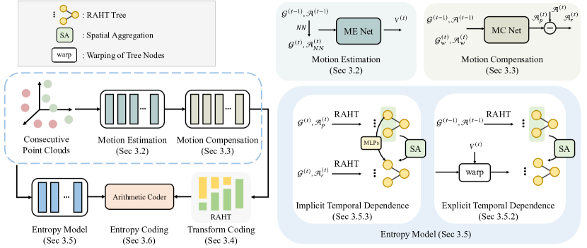
Given a point cloud sequence $\left\{\mathcal{P}^{(1)},\ldots,\mathcal{P}^{(t)}\right\}$, the point cloud geometry $\left\{\mathcal{G}^{(1)},\ldots,\mathcal{G}^{(t)}\right\}$ and the part of attributes $\left\{\mathcal{A}^{(1)},\ldots,\mathcal{A}^{(t-1)}\right\}$ are assumed to have been transmitted, and we focus on the compression of the current point cloud attributes $\mathcal{A}^{(t)}$. In Fig. 2, we present our 4DAC, a learning-based attribute compression framework for dynamic point clouds. Without loss of generality, our framework can be extended to point clouds with other attributes, such as plenoptic point clouds (Sandri et al., 2018).

As shown in Fig. 2, we first estimate 3D motion vectors from consecutive point clouds, and then perform motion compensation with the estimated 3D motion to obtain temporal attribute residuals. Next, we encode the residuals to transformed coefficients through region adaptive hierarchical transform (RAHT) (De Queiroz and Chou, 2016). In addition, we propose a deep temporal conditional entropy model to estimate distribution of transformed coefficients. Specifically, we explore implicit and explicit temporal correlations hidden in consecutive point clouds and motion estimation/compensation blocks for our deep entropy model. Finally, the coefficients and their estimated distributions are sent to an arithmetic coder to produce a compact bitstream in the entropy coding stage.

3.2. Motion Estimation

In this step, we estimate motion vectors $V^{(t)}$ from two consecutive point clouds, $\mathcal{P}^{(t-1)}$ and $\mathcal{P}^{(t)}$. The predicted motion vectors $V^{(t)}$ will be used for point cloud warping in Secs. 3.3 and 3.5.2. In order to preserve local geometry and attribute patterns of the reference point cloud $\mathcal{P}^{(t-1)}$ in the aforementioned sections, we set the motion vectors $V^{(t)}$ pointing from the current source point cloud $\mathcal{P}^{(t)}$ to the previous reference point cloud $\mathcal{P}^{(t-1)}$ and thus we can warp $\mathcal{P}^{(t)}$ instead of $\mathcal{P}^{(t-1)}$. It is also worth noting that, a relative reasonable flow estimation result can be obtained without the target attributes $\mathcal{A}^{(t)}$. Benefiting from this result, we can simply predict 3D motion information from point cloud geometry and do not need to transmit motion vectors. In particular, we feed $\left\{\mathcal{G}^{(t-1)},\mathcal{A}^{(t-1)}\right\}$ and $\left\{\mathcal{G}^{(t)},\mathcal{A}^{(t)}_{NN}\right\}$ to the flow estimation network, FlowNet3D (Liu et al., 2019), where $\mathcal{A}^{(t)}_{NN}$ is the nearest neighbor prediction from $\left\{\mathcal{G}^{(t-1)},\mathcal{A}^{(t-1)}\right\}$ to $\mathcal{G}^{(t)}$. More specifically, for each point in $\mathcal{G}^{(t)}$, we find its nearest neighbor in $\mathcal{G}^{(t-1)}$ and use the attributes of the nearest neighbor as the nearest neighbor prediction attributes.

3.3. Motion Compensation

In order to capture temporal redundancy, the motion compensation block obtains attribute residuals $\mathcal{A}^{(t)}_{r}$ from consecutive point clouds, $\mathcal{P}^{(t-1)}$ and $\mathcal{P}^{(t)}$, and the estimated motion vectors $V^{(t)}$. As mentioned in Sec. 3.2, we first warp the target point cloud geometry $\mathcal{G}^{(t)}$ with the motion vectors $V^{(t)}$, and the warped geometry $\mathcal{G}^{(t)}_{w}$ is obtained as $\mathcal{G}^{(t)}_{w}=\mathcal{G}^{(t)}+V^{(t)}$. Then, we construct a 3D attribute embedding network based on FlowNet3D (Liu et al., 2019) to estimate the target attributes $\mathcal{A}^{(t)}$. Specifically, we simply set the nearest neighbor prediction $\mathcal{A}^{(t)}_{w}$ from the $\left\{\mathcal{G}^{(t-1)},\mathcal{A}^{(t-1)}\right\}$ to $\mathcal{G}^{(t)}_{w}$ as the initial attribute prediction, and refine $\mathcal{A}^{(t)}_{w}$ to the final prediction $\mathcal{A}^{(t)}_{p}$ through the proposed network. Finally, the temporal attribute residuals $\mathcal{A}^{(t)}_{r}$ can be obtained (i.e., $\mathcal{A}^{(t)}_{r}=\mathcal{A}^{(t)}-\mathcal{A}^{(t)}_{p}$). The network architecture details of the motion estimation and compensation networks are provided in appendix.

3.4. Transform Coding

We further encode the temporal attribute residuals $\mathcal{A}^{(t)}_{r}$ into transformed coefficients $\mathcal{C}^{(t)}_{r}$ to reduce spatial redundancy. For simplicity, we use Region Adaptive Hierarchical Transform (RAHT) (De Queiroz and Chou, 2016) for transform coding. In short, RAHT is an effective 3D variant of the wavelet transform algorithm, which hierarchically decomposes attributes to DC and high-frequency coefficients. The DC coefficient is transmitted directly and the high-frequency coefficients will be further entropy coded in Sec. 3.6. This step is similar to most traditional attribute compression methods (De Queiroz and Chou, 2016; Souto and de Queiroz, 2020; Pavez et al., 2021, 2020).

According to the hierarchical transform steps, we can construct RAHT trees following (Fang et al., 2022). As shown in Fig. 3, for each point cloud in the sequence, we are able to build a RAHT tree, whose high-frequency tree nodes contain the transformed coefficients. Intuitively, there is a temporal dependence between two consecutive point clouds. Furthermore, it is also possible to extend this temporal dependence to two consecutive RAHT trees. In 3DAC (Fang et al., 2022), transform coding context and inter-channel correlation are explored via the tree structure for static point cloud attribute compression. In this paper, we further build temporal correlations within dynamic point clouds through the RAHT trees in Secs. 3.5.2 and 3.5.3. The details about RAHT and RAHT tree structure can be found in (De Queiroz and Chou, 2016; Fang et al., 2022) and the appendix.

Figure 3. A simple illustration of RAHT and RAHT tree.

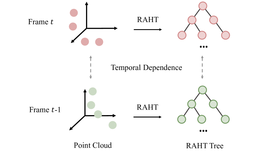
3.5. Entropy Model

The objective of the entropy model is to estimate the actual distribution of the input symbols. For dynamic point cloud attribute compression, one of the main difficulties is how to model the temporal correlations between two point clouds without direct correspondence. In this section, we propose our temporal conditional entropy model based on the RAHT tree structure. We first formulate the distribution of the transformed attribute residual coefficients $q(\mathcal{C}^{(t)}_{r})$ with temporal conditions, and then adopt neural networks to model this formulation.

3.5.1. Formulation

Given the geometry sequence $\left\{\mathcal{G}^{(1)},\ldots,\mathcal{G}^{(t)}\right\}$ and attribute sequence $\left\{\mathcal{A}^{(1)},\ldots,\mathcal{A}^{(t-1)}\right\}$, we need to compress and transmit the current attributes $\mathcal{A}^{(t)}$. After motion estimation, motion compensation and transform coding (Secs. 3.2, 3.3 and 3.4), the task has been converted to compress the transformed attribute residual coefficients $\mathcal{C}^{(t)}_{r}=\left\{\bm{c}^{(t)(1)}_{r},\ldots,\bm{c}^{(t)(m)}_{r}\right\}$. We factorize probability distribution $q(\mathcal{C}^{(t)}_{r})$ as follows:

(1) $$q(\mathcal{C}^{(t)}_{r})=\prod_{i}q\left(\bm{c}^{(t)(i)}_{r}\mid{\mathcal{G}^{(1)},\ldots,\mathcal{G}^{(t)}},{\mathcal{A}^{(1)},\ldots,\mathcal{A}^{(t-1)}}\right).$$

For simplicity, we assume the current point cloud $\mathcal{P}^{(t)}$ only depends on the previous transmitted point cloud $\mathcal{P}^{(t-1)}$. Thus, the formulation can be simplified as:

(2) $$q(\mathcal{C}^{(t)}_{r})=\prod_{i}q\left(\bm{c}^{(t)(i)}_{r}\mid{\mathcal{G}^{(t)},\mathcal{G}^{(t-1)}},{\mathcal{A}^{(t-1)}}\right).$$

Note that, it is also possible to buffer the transmitted point cloud sequence to capture more extensive temporal information.

Given the current point cloud geometry $\mathcal{G}^{(t)}$ and the previous point cloud geometry and attributes, $\mathcal{G}^{(t-1)}$ and $\mathcal{A}^{(t-1)}$, we obtained intermediate information including the motion vectors $V^{(t)}$ and the attribute prediction from motion compensation $\mathcal{A}^{(t)}_{p}$ in Secs. 3.2 and 3.3. Next, we will exploit the aforementioned context information and conclude two types of temporal context (explicit temporal dependence and implicit temporal dependence) to model the distribution $q\left(\bm{c}^{(t)(i)}_{r}\mid{\mathcal{G}^{(t)},\mathcal{G}^{(t-1)}},{\mathcal{A}^{(t-1)}}\right)$ with neural networks.

Figure 4. Our proposed temporal context. (a) Explicit temporal dependence between two consecutive point clouds, (b) Implicit temporal dependence between target attributes and prediction from motion compensation.

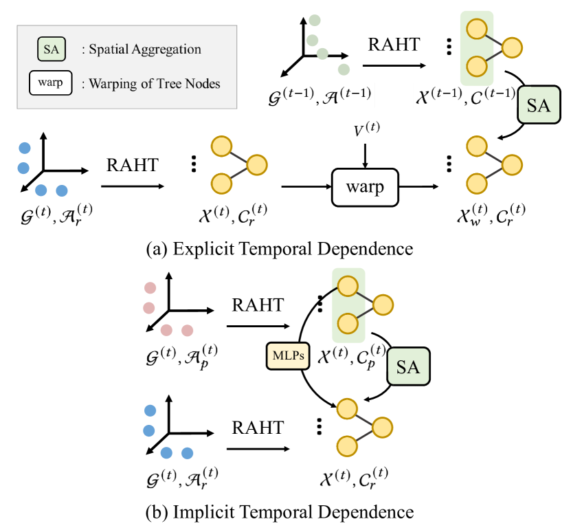
3.5.2. Explicit Temporal Dependence

Our explicit temporal dependence module explores the direct temporal correlations between two consecutive point clouds. One straightforward approach provided by MuSCLE (Biswas et al., 2020) is to extract spatial-temporal context feature by performing point convolution (Wang et al., 2018) on point cloud geometry. However, this naive temporal context aggregation method is highly based on their framework, which directly transmits point cloud attributes without transform coding. According to (Fang et al., 2022), this simple framework may limit the compression performance. Thus, in our proposed framework, we conduct temporal context feature extraction on two consecutive RAHT trees.

As shown in Fig. 4(a), we utilize the RAHT tree structure to represent dynamic point clouds. In particular, we first transform the previous point cloud $\{\mathcal{G}^{(t-1)},\mathcal{A}^{(t-1)}\}$ to a RAHT tree ${\{\mathcal{X}^{(t-1)},\mathcal{C}^{(t-1)}}\}$, where $\mathcal{X}$ and $\mathcal{C}$ denote positions and transformed coefficients of tree nodes, respectively. Similarly, attribute residual with the current geometry $\{\mathcal{G}^{(t)},\mathcal{A}^{(t)}_{r}\}$ is converted to $\{\mathcal{X}^{(t)},\mathcal{C}^{(t)}_{r}\}$. In order to minimize the spatial difference between two RAHT trees $\mathcal{X}^{(t)}$ and $\mathcal{X}^{(t-1)}$, we further warp $\mathcal{X}^{(t)}$ to $\mathcal{X}^{(t-1)}$ with the motion vectors of tree nodes. Note that, the motion vectors of tree nodes can be simply obtained as the mean value of $V^{(t)}$ in the corresponding subspace.

Then, we employ spatial aggregation to bridge two consecutive RAHT trees. Here, we have the reference RAHT tree ${\{\mathcal{X}^{(t-1)},\mathcal{C}^{(t-1)}}\}$ and the warped tree ${\{\mathcal{X}^{(t)}_{w},\mathcal{C}^{(t)}_{r}}\}$. In this step, we propose our explicit temporal context feature by exploring temporal correlations between the transmitted coefficients $\mathcal{C}^{(t-1)}$ and the transformed coefficients $\mathcal{C}^{(t)}_{r}$. It is worth noting that $\mathcal{C}^{(t)}_{r}$ is highly related to its temporal-spatial neighbors in $\mathcal{C}^{(t-1)}$. Thus, we aggregate those neighbors through PointNet++ (Qi et al., 2017b) for temporal feature aggregation. Specifically, at each depth level of RAHT trees, the explicit temporal context feature $\mathbf{E}_{i}$ can be obtained as follows:

(3) $$\mathbf{E}_{i}=\underset{j\in N(i)}{\operatorname{MAX}}\left\{MLPs\left(\bm{c}^{(t-1)(j)},\bm{x}^{(t-1)(j)}-\bm{x}_{w}^{(t)(i)}\right)\right\},$$

where $\bm{x}^{(t-1)(j)}$ and $\bm{c}^{(t-1)(j)}$ is the tree node $j$ of ${\{\mathcal{X}^{(t-1)},\mathcal{C}^{(t-1)}}\}$, and $\bm{x}^{(t)(i)}$ is tree node $i$ of $\mathcal{X}^{(t)}_{w}$. $N(i)$ is the k-nearest temporal-spatial neighbors of $\bm{x}^{(t)(i)}_{w}$ in the same depth level of $\mathcal{X}^{(t-1)}$. $MAX$ is the element-wise max pooling and $MLPs$ denotes Multi-Layer Perceptrons.

3.5.3. Implicit Temporal Dependence

Our implicit temporal dependence module incorporates intermediate temporal information hidden in 3D motion processing parts. Considering this type of temporal information is extracted from dynamic points indirectly, we denote it as implicit temporal context in contrast to the aforementioned explicit temporal context. Here, we make use of attribute prediction $\mathcal{A}^{(t)}_{p}$ from our motion compensation network to estimate $\mathcal{A}^{(t)}_{r}$. As shown in Fig. 4(b), point clouds $\{\mathcal{G}^{(t)},\mathcal{A}^{(t)}_{p}\}$ and $\{\mathcal{G}^{(t)},\mathcal{A}^{(t)}_{r}\}$ are firstly transformed to RAHT trees ${\{\mathcal{X}^{(t)},\mathcal{C}^{(t)}_{p}}\}$ and ${\{\mathcal{X}^{(t)},\mathcal{C}^{(t)}_{r}}\}$. Note that, these two RAHT trees share the same spatial structure $\mathcal{X}^{(t)}$. In other words, the attribute prediction and the residual coefficients, $\bm{c}_{p}^{(t)(i)}$ and $\bm{c}_{r}^{(t)(i)}$, share the same tree node $i$. Thus, we extract latent node feature $\mathbf{N}_{i}$ from $\bm{c}_{p}^{(t)(i)}$ with MLPs:

(4) $$\mathbf{N}_{i}=MLPs\left(\bm{c}_{p}^{(t)(i)}\right).$$

We can also extract spatial feature $\mathbf{S}_{i}$ within the RAHT tree through point convolution:

(5) $$\mathbf{S}_{i}=\underset{j\in N(i)}{\operatorname{MAX}}\left\{MLPs\left(\bm{c}^{(t)(j)}_{p},\bm{x}^{(t)(j)}-\bm{x}^{(t)(i)}\right)\right\}.$$

Finally, we fuse $\mathbf{N}_{i}$ and $\mathbf{S}_{i}$ to obtain our implicit temporal context embedding $\mathbf{I}_{i}$:

(6) $$\mathbf{I}_{i}=MLPs\left(\mathbf{N}_{i},\mathbf{S}_{i}\right).$$

3.5.4. Probability Estimation

We further aggregate the context features and adopt a probability model (Ballé et al., 2018) to model the distribution of residual coefficients. In particular, we feed two temporal context features $\mathbf{E}_{i}$ and $\mathbf{I}_{i}$ into MLPs and incorporate the generated feature into a fully factorized density model (Ballé et al., 2018), which model the distribution $q\left(\bm{c}^{(t)(i)}_{r}\mid{\mathcal{G}^{(t)},\mathcal{G}^{(t-1)}},{\mathcal{A}^{(t-1)}}\right)$ as $q\left(\bm{c}^{(t)(i)}_{r}\mid{\mathbf{E}_{i},\mathbf{I}_{i}}\right)$.

3.6. Entropy Coding

At the entropy coding stage, we feed the coefficients $\mathcal{C}^{(t)}_{r}$ and their corresponding distribution $q\left(\bm{c}^{(t)(i)}_{r}\mid{\mathbf{E}_{i},\mathbf{I}_{i}}\right)$ to an arithmetic coder to produce the final attribute bitstream.

3.7. Learning

During training, we optimize our motion estimation network, motion compensation network and deep entropy model jointly. We adopt L2 loss for both motion estimation and compensation:

(7) $$\mathrm{L}_{\mathrm{ME}}=\frac{1}{m}\sum_{i}^{m}\left\{\left(v_{p}^{(t)(i)}-v_{gt}^{(t)(i)}\right)^{2}\right\},$$

where $v_{gt}^{(t)(i)}$ and $v_{p}^{(t)(i)}$ are the ground truth motion vector and the predicted motion vector of point $i$ in the point cloud $\mathcal{P}^{(t)}$, and

(8) $$\mathrm{L}_{\mathrm{MC}}=\frac{1}{m}\sum_{i}^{m}\left\{\left(\bm{a}_{p}^{(t)(i)}-\bm{a}_{gt}^{(t)(i)}\right)^{2}\right\},$$

where $\bm{a}_{gt}^{(t)(i)}$ and $\bm{a}_{p}^{(t)(i)}$ are the ground truth attributes and the predicted attributes of the point $i$. For our deep entropy model, we use the cross-entropy loss:

(9) $$\mathrm{L}_{\mathrm{CE}}=-\sum_{i}\log q(\bm{c}_{r}^{(t)(i)}\mid\mathbf{E}_{i},\mathbf{I}_{i}).$$

Thus, the total loss $\mathrm{L}_{\mathrm{total}}$ is composed of the motion estimation loss $\mathrm{L}_{\mathrm{ME}}$, the motion compensation loss $\mathrm{L}_{\mathrm{MC}}$ and the cross entropy loss $\mathrm{L}_{\mathrm{CE}}$:

(10) $$\mathrm{L}_{\mathrm{total}}=\mathrm{L}_{\mathrm{CE}}+\lambda_{\text{ME }}\mathrm{L}_{\mathrm{ME}}+\lambda_{\text{MC }}\mathrm{L}_{\mathrm{MC}},$$

where $\lambda_{\text{ME }}$ and $\lambda_{\text{MC }}$ are set to 1.0 empirically.

4. Experiments

We evaluate our 4DAC first quantitatively and then qualitatively on several dynamic point cloud datasets. Then, we include two downstream tasks to further demonstrate the effectiveness of our proposed method. We also conduct extensive ablation studies on each component of our framework.

4.1. Experimental Setup

(1) Datasets. For evaluation of our method, we use three benchmark datasets as follows:

• FlyingThings3D (Mayer et al., 2016; Liu et al., 2019). This is a dynamic point cloud dataset generated by scenes with moving objects in ShapeNet (Chang et al., 2015). This dataset contains 22k pairs of colored point clouds with ground truth motion vectors. Following the official training/testing split (Liu et al., 2019), we use 20k of them for training and 2k for test.

• MVUB (Loop et al., 2016). This is a dynamic point cloud dataset introduced by (De Queiroz and Chou, 2016). There are five subject sequences in the dataset, named as ”Andrew”, ”David”, ”Ricardo”, ”Phil” and ”Sarah”. These colored point cloud sequences are generated by RGBD cameras with a voxelization algorithm (Loop et al., 2013). Each sequence contains 200 to 300 point clouds. We use ”Andrew”, ”David” and ”Ricardo” for training, and ”Phil” and ”Sarah” for test.

• 8iVFB (d’Eon et al., 2017). This is a MPEG/JPEG point cloud compression dataset containing four human point cloud sequences, including ”Soldier”, ”Longdress”, ”Loot” and ”Redandblack”. Each point cloud sequence is captured by RGB cameras and contains 300 dense point clouds. We use ”Soldier” and ”Longdress” for training, and others for test.

(2) Evaluation Metrics. Following (De Queiroz and Chou, 2016), we report the Peak Signal-to-Noise Ratio of the luminance component ($\rm{PSNR}_{y}$) and Bits Per Point ($\rm BPP$) to evaluate the reconstruction quality and the compression ratio, respectively.

(3) Baselines. We compare our 4DAC with several baselines:

• RAHT (De Queiroz and Chou, 2016). This is a baseline method for both static and dynamic point cloud attribute compression. Following the original implementation in (De Queiroz and Chou, 2016), we use RAHT for transform coding and the run-length Golomb-Rice coder (Malvar, 2006) for entropy coding.

• NN-RAHT. This is a baseline method for dynamic point cloud attribute compression. Based on the aforementioned RAHT, we additionally include nearest neighbor prediction. More specifically, we assume the motion vectors of point clouds equal to zero and adopt nearest neighbor for motion estimation and motion compensation. The attribute residual is further encoded by RAHT and a run-length Golomb-Rice coder.

• G-PCC (Schwarz et al., 2018). This is a MPEG standard point cloud compression software . G-PCC supports three transform coding methods and several other options. For a fair comparison, we choose RAHT without inter-depth prediction for transform coding.

• 3DAC (Fang et al., 2022). This is a state-of-the-art learning-based attribute compression method focusing on static point clouds. In 3DAC (Fang et al., 2022), RAHT is adopted for transform coding and a tree-structured deep entropy model is proposed for entropy coding.

Note that, we also conduct experiments on other learning-based attribute compression methods on our benchmarks. Considering that the results of these methods are beyond the common quality comparison range (i.e., low $\rm{PSNR}_{y}$ with high $\rm BPP$), we separately present them in appendix for better illustration.

Figure 5. Quantitative results on FlyingThings3D (a), MVUB ”Phil”(b), MVUB ”Sarah”(c), 8iVFB ”Loot” (d) and 8iVFB ”Redandblack” (e).

Figure 6. Experiments about the training dataset and our proposed modules. (a) Effect of the training dataset. We train models on the training set of 8iVFB and ”Redandblack”, respectively, and evaluate them on the test set of ”Redandblack”. (b) Ablation study on FlyingThings3D. We add motion estimation, motion compensation and entropy model one by one, and report the corresponding attribute compression performance.

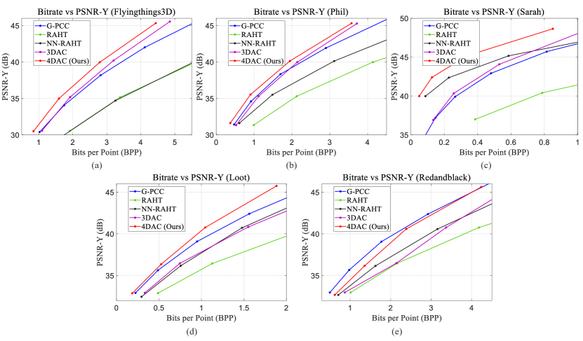
(4) Implementation Details. In the common case of point cloud compression, point cloud geometry and attributes are usually compressed and transmitted separately. To simulate this real condition in our experiments, we use a 9-level octree to voxelize the raw point cloud data and assume the point cloud geometry has been transmitted independently. For all datasets, we convert point cloud colors from the RGB color space to the YUV color space following the default setting of G-PCC (Schwarz et al., 2018). Because there is no ground truth motion vector in the MVUB and 8iVFB datasets, we adopt a pseudo motion vector as the ground truth $v_{gt}^{(t)}$ in Eq. 7. More specifically, for a point in the current point cloud frame, we search its nearest neighbor in the previous point cloud through spatial and color space (i.e., xyzrgb) and use the spatial displacement between two points as the pseudo motion vector. Note that, more advanced methods, such as self-supervised scene flow estimation, can be utilized, which is beyond the scope of this paper. Considering that our 4DAC and the previous 3DAC (Fang et al., 2022) share the similar transform coding and entropy coding blocks, we further include context features of 3DAC with our temporal context.

4.2. Evaluation on Public Datasets

Figure 5 shows the quantitative attribute compression results on FlyingThings3D, MVUB (sequences ”Phil” and ”Sarah”) and 8iVFB (sequences ”Loot” and ”Redandblack”). We can see that NN-RAHT outperforms RAHT on MVUB and 8iVFB because these datasets contain point clouds with relative small motion. However, on FlyingThings3D, nearest neighbor motion estimation has no positive effect due to the relative large motion of dynamic point cloud pairs. In contrast, our 4DAC consistently outperforms its static counterpart, 3DAC, by a large margin on all benchmarks, which shows the effectiveness of our dynamic compression framework. Overall, our method achieves competitive compression performance compared with other baselines on most datasets except ”Redandblack”. The main reason is that the color distribution of ”Redandblack” is different from our training sequences (i.e., ”Soldier” and ”Longdress”).

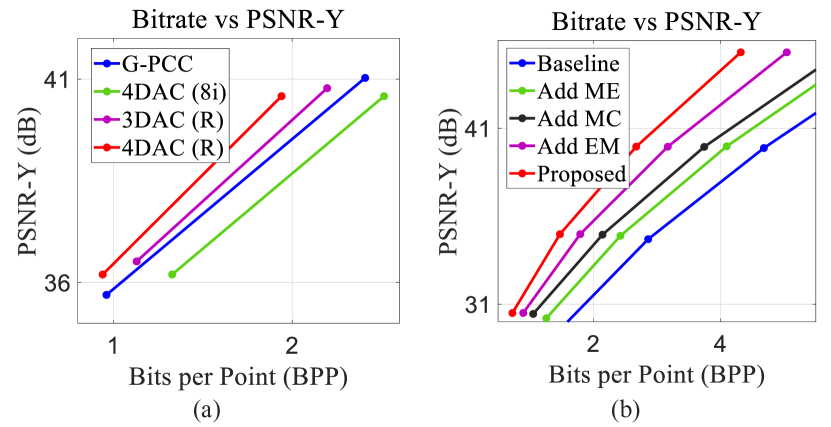
To validate this assumption, we adopt a train-val-test split of [50%, 20%, 30%] on the sequence ”Redandblack”. Note that, point clouds in the sequence is not shuffled, and thus we can simulate a use case that we are compressing subsequent point cloud frames with a transmitted point cloud sequence. The result is shown in Fig. 6(a), 3DAC (R) and 4DAC (R) denote 3DAC and 4DAC trained on the train split of ”Redandblack”, and 4DAC (8i) is 4DAC trained on ”Soldier” and ”Longdress” of 8iVFB. Both 3DAC (R) and 4DAC (R) outperform G-PCC and 4DAC (8i), which shows the effect of the training dataset. One simple but practical solution is to enlarge the scale of the training dataset to minimize the domain gap between the training and test splits.

We also provide the qualitative results on ”Loot” with the corresponding quantitative results in Fig. 7. The results on other datasets are provided in appendix. It is obvious that our method outperforms other attribute compression methods, which is consistent to the quantitative results.

Figure 7. Qualitative results of our 4DAC and other baselines. The quantitative results ($\rm BPP$, $\rm{PSNR}_{y}$, $\rm GraphSIM$) are also shown under the figure. our 4DAC achieves the best reconstruction quailty ($\rm{PSNR}_{y}$ and $\rm GraphSIM$) with the lowest bitrate.

Figure 8. The experiment results on two downstream tasks. (a) Scene flow estimation on FlyingThings3D. (b) Quality asessment on ”Loot”.

4.3. Evaluation on Downstream Tasks

In order to validate the compression performance on downstream tasks, we conduct experiments on scene flow estimation and quality assessment for machine and human perception, respectively.

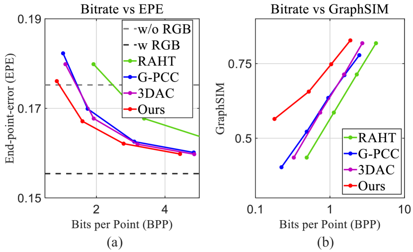
Scene Flow Estimation. Figure 8(a) shows the downstream performance on FlyingThings3D with FlowNet3D (Liu et al., 2019). Following (Fang et al., 2022), we train the network on the raw point clouds and evaluate it with the compressed target point cloud. End-point-error (EPE) at different $\rm BPP$s is used as the evaluation metric, and the results of raw point clouds with and without attributes are denoted as ‘w RGB’ and ‘w/o RGB’, respectively. It is obvious that our 4DAC outperforms 3DAC and G-PCC, which demonstrates the superior compression performance of our method on this downstream task.

Quality Assessment. We adopt the point cloud quality assessment task to show the effectiveness of our method on human perception. In particular, we use GraphSIM (Yang et al., 2020) to evaluate the point cloud attribute reconstruction quality. As an attribute-sensitive metric, a higher GraphSIM score means better reconstruction quality. As shown in Fig. 8(b), with the help of temporal information, our approach outperforms other baselines by a large margin. This experimental result further demonstrates the effectiveness of our method.

4.4. Ablation Study

In this section, we conduct ablation studies on each component of our dynamic attribute compression framework to show their effect on the compression performance. As shown in Fig. 6(b), we include several results by adding our proposed components progressively. In particular, we construct a basic baseline method with RHAT as transform coding and a fully factorized density model (Ballé et al., 2018) as entropy model, and denote it as ‘Baseline’. Wu further construct ‘Add ME’, ‘Add MC’, ‘Add EM’ by adding motion estimation, motion compensation, deep entropy model with temporal context. We additionally incorporate 3DAC context and denote the final framework as ‘proposed’. Experiments are conducted on FlyingThings3D with different $\rm BPP$s. The performance shown in Fig. 6(b) demonstrates that our framework can achieve a much lower bitrate with the similar reconstruction quality with the help of our proposed components. Besides, the result also indicates that our 4DAC can perform well with the previous state-of-the-art compression algorithm, 3DAC (Fang et al., 2022). It shows the possibility for our framework to incorporate with more advanced algorithms for a better compression performance.

We also report the ablation studies on our temporal context features for our deep entropy model in Table 1. Specifically, we also conduct experiments on FlyingThings3D and set the uniform quantization parameter as 10 for the same reconstruction quality. We progressively incorporate explicit temporal context (E), implicit temporal context (I) and 3DAC context (3DAC), and it can be seen that the bitrate is steadily reduced with incorporation of more context features, which shows the effectiveness of our proposed explicit and implicit temporal dependence modules.

E	I	3DAC	Birate
			3.74
$\checkmark$			3.53
$\checkmark$	$\checkmark$		3.17
$\checkmark$	$\checkmark$	$\checkmark$	2.67

Table 1. Ablation study on context features for entropy model. E, I and 3DAC denote explicit temporal context, implicit temporal context and 3DAC context (Fang et al., 2022), respectively.

5. Conclusion

We have presented a dynamic point cloud attribute compression framework. This framework includes a motion estimation block, a motion compensation block and a temporal conditional entropy model to leverage temporal information within data. Besides, our deep entropy model exploits explicit and implicit temporal dependence to model the probability distribution. Furthermore, we show the competitive performance of our method on several datasets, and the results on downstream tasks show that our algorithm is capable for both machine and human perception tasks.

Appendix

Appendix A Additional Method Details

A.1. Motion Estimation and Compensation

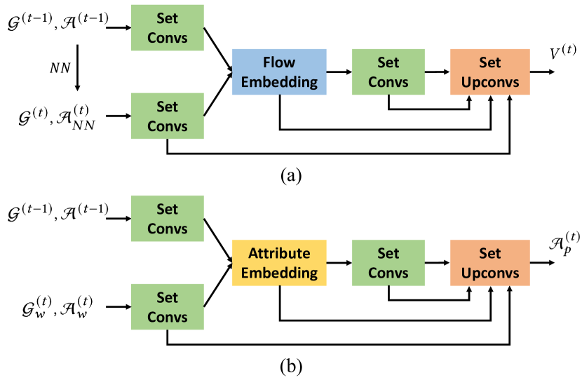
The motion estimation network and the motion compensation network are shown in Fig. 9. We construct our motion estimation and motion compensation nets with modules (Set Conv, Flow Embedding and Set Upconv) proposed by FlowNet3D (Liu et al., 2019). Because the motion compensation net extracts point cloud attribute information rather than motion information, we denote the attribute feature fusion module (the yellow block in Fig. 9(b)) as Attribute Embedding instead of Flow Embedding although they share the similar architecture.

A.2. Transform Coding

In this paper, we use Region Adaptive Hierarchical Transform (RAHT) (De Queiroz and Chou, 2016) for transform coding. In the following parts, we first introduce RAHT, and then show how to construct a RAHT tree.

A.2.1. Region Adaptive Hierarchical Transform

RAHT transforms point cloud attributes to frequency-domain coefficients based on 3D Haar wavelet transform. Specifically, the algorithm takes a voxelized point cloud as input, and convert attributes to low- and high-frequency coefficients along three dimensions repeatedly. Different from the common 2D wavelet transform, RAHT is able to process empty spaces through transmitting low-frequency coefficients to the next depth level directly. Besides, the wavelet basis of RAHT is adaptive to the number of points in the corresponding region. More specifically, two low-frequency neighbors are decomposed to low- and high-frequency coefficients as follows:

(11) $$\left[\begin{array}[]{c}l_{d+1,x,y,z}\\ h_{d+1,x,y,z}\end{array}\right]=\frac{1}{\sqrt{w_{1}+w_{2}}}\left[\begin{array}[]{cc}\sqrt{w_{1}}&\sqrt{w_{2}}\\ -\sqrt{w_{2}}&\sqrt{w_{1}}\end{array}\right]\left[\begin{array}[]{c}l_{d,2x,y,z}\\ l_{d,2x+1,y,z}\end{array}\right],$$

where $l_{d,2x,y,z}$ and $l_{d,2x+1,y,z}$ are two low-frequency neighbors along the $x$ dimension, and $w_{1}$ and $w_{2}$ are their weights (i.e., the number of points in the corresponding subspace). $l_{d+1,x,y,z}$ and $h_{d+1,x,y,z}$ are the decomposed low- and high-frequency coefficients, respectively.

Figure 9. The proposed Motion Estimation Net (a) and Motion Compensation Net (b).

Figure 10. A 2D example of RAHT. (a) Point cloud. (b) The transform steps of RAHT. (C) The corresponding RAHT tree.

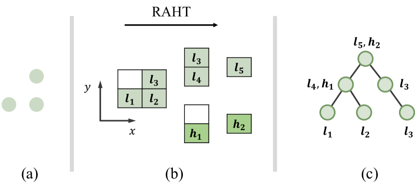
A.2.2. RAHT Tree

We revisit the transform process of RAHT and the construction of a RAHT tree through a 2D toy example in Fig. 10. The input point cloud is first voxlized and then transformed. Low- and high-frequency coefficients are denoted as $l_{i}$ and $h_{i}$, respectively. During encoding, transform is conducted along the $x$ axis and then the $y$ axis repeatedly until all voxelized points are merged. At the first depth level, along the $x$ axis, point without neighbor (i.e., $l_{3}$), is transmitted to the next depth level and those with a neighbor (i.e., $l_{1}$ and $l_{2}$) are decomposed to low- and high-frequency coefficients (i.e., $l_{4}$ and $h_{1}$). In this way, we transform low-frequency coefficients depth by depth until generating the DC coefficient $l_{5}$. After forward transform, we compress the DC coefficient and all high-frequency coefficients, and thus, during decoding, we can recover all low-frequency coefficients. Specifically, decoding is start from the root level. We can reconvert the DC coefficient $l_{5}$ and high-frequency coefficient $h_{2}$ to low-frequency coefficients of the previous depth (i.e., $l_{3}$ and $l_{4}$). In this way, all low-frequency coefficients can be regenerated depth by depth.

Here, we further construct the RAHT tree of the aforementioned toy example. Following the hierarchical transform processes, the RAHT tree is constructed as Fig. 10(c). Low-frequency coefficients of the first depth level (i.e., point cloud attributes), $l_{1}$, $l_{2}$ and $l_{3}$, are set as leaf nodes. These tree nodes are transmitted or merged according to the repeated transform steps. Specifically, tree nodes of $l_{1}$ and $l_{2}$ are merged to that of $l_{4}$ and $h_{1}$, and tree nodes of $l_{4}$ and $l_{3}$ are merged to that of $l_{5}$ and $h_{2}$.

Appendix B Additional Implementation Details

We pretrain the motion estimation and compensation networks first and then train these two networks with our deep entropy model jointly. For faster convergence of the motion estimation net, we initialize the estimated motion vectors $V^{(t)}$ as zeros. In specific, we multiply the output vectors of the motion estimation net with learnable tensors which are initialized as zeros, and use the result as the estimated motion vectors $V^{(t)}$. For our motion compensation net, we initialize the predicted attributes $\mathcal{A}^{(t)}_{p}$ as the input attributes $\mathcal{A}^{(t)}_{w}$. In specific, we multiply the output vectors of the motion compensation net with learnable tensors (which are also initialized as zeros), and add them with the input attributes. The result is regarded as the the predicted attributes. For Explicit Temporal Dependence, we aggregate temporal features from 3 nearset neighbors through 3-layer MLPs (16, 32 and 8 dimensional hidden features). For Implicit Temporal Dependence, we extract latent node feature $\mathbf{N}_{i}$ with 3-layer MLPs (16, 32 and 8) and spatial feature $\mathbf{S}_{i}$ from 3 nearset neighbors with 3-layer MLPs (16, 32 and 8), then we fuse the node feature and spatial feature to our implicit temporal context embedding $\mathbf{I}_{i}$ with a MLP (8). Finally, the explicit and implicit context features are concatenated with the 3DAC context feature for our deep entropy model.

Appendix C Additional Experiments

C.1. Comparison with Learning-based Methods

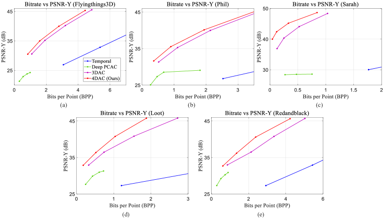
We also compare our 4DAC with several learning-based attribute compression methods. Specifically, we additionally present the performance of DeepPCAC (Sheng et al., 2021) and Temporal. DeepPCAC is a static attribute compression method which constructs the transform coding block and the entropy model with point-based auto-encoders (Qi et al., 2017b). Temporal is a simple dynamic attribute compression framework only containing a deep entropy model and an entropy coder. The entropy model extracts context feature from the previous point cloud through spatial-temporal aggregation inspired by (Biswas et al., 2020). As shown in Fig. 11, our 4DAC significantly outperforms existing learning-based methods. This result demonstrates the effectiveness of our proposed method.

C.2. Additional Qualitative Results

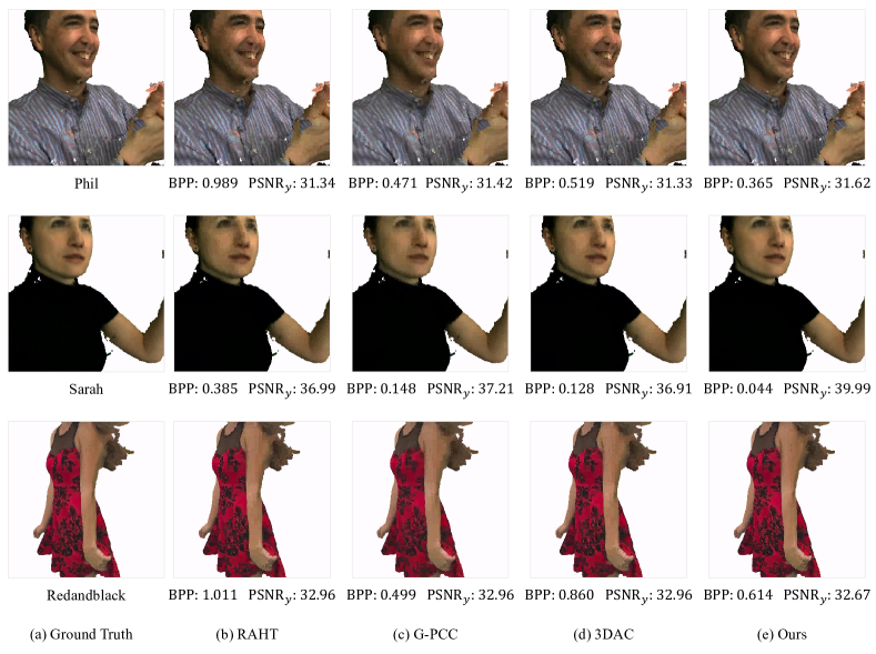
In Fig. 12, We present additional qualitative results on MVUB ”Phil”, MVUB ”Sarah” and 8iVFB ”Redandblack”. The corresponding $\rm BPP$ and $\rm{PSNR}_{y}$ of the sequence are also provided. It shows that our method can achieve better reconstruction quality with the help of the temporal information.

Figure 11. The quantitative results compared with learning-based methods.

Figure 12. Additional qualitative results.

References

- (1)
- Achlioptas et al. (2018) Panos Achlioptas, Olga Diamanti, Ioannis Mitliagkas, and Leonidas Guibas. 2018. Learning representations and generative models for 3D point clouds. In ICML. PMLR, 40–49.
- Agustsson et al. (2020) Eirikur Agustsson, David Minnen, Nick Johnston, Johannes Balle, Sung Jin Hwang, and George Toderici. 2020. Scale-space flow for end-to-end optimized video compression. In CVPR. 8503–8512.
- Alexiou et al. (2020) Evangelos Alexiou, Kuan Tung, and Touradj Ebrahimi. 2020. Towards neural network approaches for point cloud compression. In Applications of Digital Image Processing XLIII, Vol. 11510. SPIE, 18–37.
- Ballé et al. (2018) Johannes Ballé, David Minnen, Saurabh Singh, Sung Jin Hwang, and Nick Johnston. 2018. Variational image compression with a scale hyperprior. In ICLR.
- Biswas et al. (2020) Sourav Biswas, Jerry Liu, Kelvin Wong, Shenlong Wang, and Raquel Urtasun. 2020. MuSCLE: Multi Sweep Compression of LiDAR using Deep Entropy Models. NeurIPS 33 (2020).
- Brock et al. (2016) Andrew Brock, Theodore Lim, James Millar Ritchie, and Nicholas J Weston. 2016. Generative and Discriminative Voxel Modeling with Convolutional Neural Networks. In Neural Inofrmation Processing Conference: 3D Deep Learning.
- Bross et al. (2021) Benjamin Bross, Jianle Chen, Jens-Rainer Ohm, Gary J Sullivan, and Ye-Kui Wang. 2021. Developments in international video coding standardization after avc, with an overview of versatile video coding (vvc). Proc. IEEE 109, 9 (2021), 1463–1493.
- Chang et al. (2015) Angel X Chang, Thomas Funkhouser, Leonidas Guibas, Pat Hanrahan, Qixing Huang, Zimo Li, Silvio Savarese, Manolis Savva, Shuran Song, Hao Su, et al. 2015. ShapeNet: An information-rich 3D model repository. arXiv preprint arXiv:1512.03012 (2015).
- Choy et al. (2019) Christopher Choy, JunYoung Gwak, and Silvio Savarese. 2019. 4D Spatio-Temporal ConvNets: Minkowski Convolutional Neural Networks. In CVPR. IEEE, 3070–3079.
- De Queiroz and Chou (2016) Ricardo L De Queiroz and Philip A Chou. 2016. Compression of 3D point clouds using a region-adaptive hierarchical transform. IEEE TIP 25, 8 (2016), 3947–3956.
- De Queiroz and Chou (2017) Ricardo L De Queiroz and Philip A Chou. 2017. Motion-compensated compression of dynamic voxelized point clouds. IEEE TIP 26, 8 (2017), 3886–3895.
- Dorea and de Queiroz (2018) Camilo Dorea and Ricardo L de Queiroz. 2018. Block-based motion estimation speedup for dynamic voxelized point clouds. In ICIP. IEEE, 2964–2968.
- Dorea et al. (2019) Camilo Dorea, Edson M Hung, and Ricardo L de Queiroz. 2019. Local texture and geometry descriptors for fast block-based motion estimation of dynamic voxelized point clouds. In ICIP. IEEE, 3721–3725.
- Dosovitskiy et al. (2015) Alexey Dosovitskiy, Philipp Fischer, Eddy Ilg, Philip Hausser, Caner Hazirbas, Vladimir Golkov, Patrick Van Der Smagt, Daniel Cremers, and Thomas Brox. 2015. FlowNet: Learning optical flow with convolutional networks. In ICCV. 2758–2766.
- d’Eon et al. (2017) Eugene d’Eon, Bob Harrison, Taos Myers, and Philip A Chou. 2017. 8i voxelized full bodies-a voxelized point cloud dataset. ISO/IEC JTC1/SC29 Joint WG11/WG1 (MPEG/JPEG) input document WG11M40059/WG1M74006 7 (2017), 8.
- Fang et al. (2022) Guangchi Fang, Qingyong Hu, Hanyun Wang, Yiling Xu, and Guo Yulan. 2022. 3DAC: Learning Attribute Compression for Point Clouds. arXiv preprint arXiv:2203.09931 (2022).
- Fu et al. (2022) Chunyang Fu, Ge Li, Rui Song, Wei Gao, and Shan Liu. 2022. OctAttention: Octree-based Large-scale Contexts Model for Point Cloud Compression. arXiv preprint arXiv:2202.06028 (2022).
- Gao et al. (2021) Linyao Gao, Tingyu Fan, Jianqiang Wan, Yiling Xu, Jun Sun, and Zhan Ma. 2021. Point Cloud Geometry Compression Via Neural Graph Sampling. In ICIP. IEEE, 3373–3377.
- Garcia et al. (2019) Diogo C Garcia, Tiago A Fonseca, Renan U Ferreira, and Ricardo L de Queiroz. 2019. Geometry coding for dynamic voxelized point clouds using octrees and multiple contexts. IEEE TIP 29 (2019), 313–322.
- Geiger et al. (2012) Andreas Geiger, Philip Lenz, and Raquel Urtasun. 2012. Are we ready for autonomous driving? the KITTI vision benchmark suite. In CVPR. 3354–3361.
- Gojcic et al. (2021) Zan Gojcic, Or Litany, Andreas Wieser, Leonidas J Guibas, and Tolga Birdal. 2021. Weakly supervised learning of rigid 3D scene flow. In CVPR. 5692–5703.
- Gu et al. (2019) Shuai Gu, Junhui Hou, Huanqiang Zeng, Hui Yuan, and Kai-Kuang Ma. 2019. 3D point cloud attribute compression using geometry-guided sparse representation. IEEE TIP 29 (2019), 796–808.
- Hu et al. (2021b) Qingyong Hu, Bo Yang, Linhai Xie, Stefano Rosa, Yulan Guo, Zhihua Wang, Niki Trigoni, and Andrew Markham. 2021b. Learning Semantic Segmentation of Large-Scale Point Clouds with Random Sampling. IEEE TPAMI (2021).
- Hu et al. (2021a) Zhihao Hu, Guo Lu, and Dong Xu. 2021a. FVC: A new framework towards deep video compression in feature space. In CVPR. 1502–1511.
- Huang et al. (2020) Lila Huang, Shenlong Wang, Kelvin Wong, Jerry Liu, and Raquel Urtasun. 2020. OctSqueeze: Octree-structured entropy model for lidar compression. In CVPR. 1313–1323.
- Huang and Liu (2019) Tianxin Huang and Yong Liu. 2019. 3D point cloud geometry compression on deep learning. In ACM MM. 890–898.
- Ilg et al. (2017) Eddy Ilg, Nikolaus Mayer, Tonmoy Saikia, Margret Keuper, Alexey Dosovitskiy, and Thomas Brox. 2017. FlowNet 2.0: Evolution of optical flow estimation with deep networks. In CVPR. 2462–2470.
- Isik et al. (2021) Berivan Isik, Philip A Chou, Sung Jin Hwang, Nick Johnston, and George Toderici. 2021. LVAC: Learned Volumetric Attribute Compression for Point Clouds using Coordinate Based Networks. arXiv preprint arXiv:2111.08988 (2021).
- Kammerl et al. (2012) Julius Kammerl, Nico Blodow, Radu Bogdan Rusu, Suat Gedikli, Michael Beetz, and Eckehard Steinbach. 2012. Real-time compression of point cloud streams. In ICRA. IEEE, 778–785.
- Kittenplon et al. (2021) Yair Kittenplon, Yonina C Eldar, and Dan Raviv. 2021. FlowStep3D: Model unrolling for self-supervised scene flow estimation. In CVPR. 4114–4123.
- Li et al. (2021) Bing Li, Cheng Zheng, Silvio Giancola, and Bernard Ghanem. 2021. SCTN: Sparse convolution-transformer network for scene flow estimation. arXiv preprint arXiv:2105.04447 (2021).
- Liu et al. (2019) Xingyu Liu, Charles R Qi, and Leonidas J Guibas. 2019. FlowNet3D: Learning scene flow in 3D point clouds. In CVPR. 529–537.
- Loop et al. (2016) Charles Loop, Qin Cai, S Orts Escolano, and Philip A Chou. 2016. Microsoft voxelized upper bodies-a voxelized point cloud dataset. ISO/IEC JTC1/SC29 Joint WG11/WG1 (MPEG/JPEG) input document m38673 M 72012 (2016), 2016.
- Loop et al. (2013) Charles Loop, Cha Zhang, and Zhengyou Zhang. 2013. Real-time high-resolution sparse voxelization with application to image-based modeling. In Proceedings of the 5th High-performance Graphics Conference. 73–79.
- Lu et al. (2019) Guo Lu, Wanli Ouyang, Dong Xu, Xiaoyun Zhang, Chunlei Cai, and Zhiyong Gao. 2019. DVC: An end-to-end deep video compression framework. In CVPR. 11006–11015.
- Malvar (2006) Henrique S Malvar. 2006. Adaptive run-length/Golomb-Rice encoding of quantized generalized Gaussian sources with unknown statistics. In DCC. IEEE, 23–32.
- Mayer et al. (2016) Nikolaus Mayer, Eddy Ilg, Philip Hausser, Philipp Fischer, Daniel Cremers, Alexey Dosovitskiy, and Thomas Brox. 2016. A large dataset to train convolutional networks for disparity, optical flow, and scene flow estimation. In CVPR. 4040–4048.
- Meagher (1982) Donald Meagher. 1982. Geometric modeling using octree encoding. Computer graphics and image processing 19, 2 (1982), 129–147.
- Mekuria et al. (2016) Rufael Mekuria, Kees Blom, and Pablo Cesar. 2016. Design, implementation, and evaluation of a point cloud codec for tele-immersive video. TCSVT 27, 4 (2016), 828–842.
- Pan et al. (2006) Zhigeng Pan, Adrian David Cheok, Hongwei Yang, Jiejie Zhu, and Jiaoying Shi. 2006. Virtual reality and mixed reality for virtual learning environments. Computers & graphics 30, 1 (2006), 20–28.
- Pavez et al. (2020) Eduardo Pavez, Benjamin Girault, Antonio Ortega, and Philip A Chou. 2020. Region adaptive graph Fourier transform for 3D point clouds. In ICIP. IEEE, 2726–2730.
- Pavez et al. (2021) Eduardo Pavez, Andre L Souto, Ricardo L De Queiroz, and Antonio Ortega. 2021. Multi-resolution intra-predictive coding of 3D point cloud attributes. arXiv preprint arXiv:2106.08562 (2021).
- Qi et al. (2017a) Charles R Qi, Hao Su, Kaichun Mo, and Leonidas J Guibas. 2017a. PointNet: Deep learning on point sets for 3D classification and segmentation. In CVPR. 652–660.
- Qi et al. (2017b) Charles Ruizhongtai Qi, Li Yi, Hao Su, and Leonidas J Guibas. 2017b. PointNet++: Deep hierarchical feature learning on point sets in a metric space. In NeurIPS.
- Quach et al. (2019) Maurice Quach, Giuseppe Valenzise, and Frederic Dufaux. 2019. Learning convolutional transforms for lossy point cloud geometry compression. In ICIP. IEEE, 4320–4324.
- Quach et al. (2020) Maurice Quach, Giuseppe Valenzise, and Frederic Dufaux. 2020. Improved deep point cloud geometry compression. In MMSP. IEEE, 1–6.
- Que et al. (2021) Zizheng Que, Guo Lu, and Dong Xu. 2021. VoxelContext-Net: An Octree based Framework for Point Cloud Compression. In CVPR. 6042–6051.
- Rippel et al. (2019) Oren Rippel, Sanjay Nair, Carissa Lew, Steve Branson, Alexander G Anderson, and Lubomir Bourdev. 2019. Learned video compression. In ICCV. 3454–3463.
- Sandri et al. (2018) Gustavo Sandri, Ricardo L de Queiroz, and Philip A Chou. 2018. Compression of plenoptic point clouds. IEEE TIP 28, 3 (2018), 1419–1427.
- Schwarz et al. (2007) Heiko Schwarz, Detlev Marpe, and Thomas Wiegand. 2007. Overview of the scalable video coding extension of the H. 264/AVC standard. TCSVT 17, 9 (2007), 1103–1120.
- Schwarz et al. (2018) Sebastian Schwarz, Marius Preda, Vittorio Baroncini, Madhukar Budagavi, Pablo Cesar, Philip A Chou, Robert A Cohen, Maja Krivokuća, Sébastien Lasserre, Zhu Li, et al. 2018. Emerging MPEG standards for point cloud compression. IEEE Journal on Emerging and Selected Topics in Circuits and Systems 9, 1 (2018), 133–148.
- Shao et al. (2018) Yiting Shao, Qi Zhang, Ge Li, Zhu Li, and Li Li. 2018. Hybrid point cloud attribute compression using slice-based layered structure and block-based intra prediction. In ACM MM. 1199–1207.
- Shao et al. (2017) Yiting Shao, Zhaobin Zhang, Zhu Li, Kui Fan, and Ge Li. 2017. Attribute compression of 3D point clouds using Laplacian sparsity optimized graph transform. In VCIP. IEEE, 1–4.
- Sheng et al. (2021) Xihua Sheng, Li Li, Dong Liu, Zhiwei Xiong, Zhu Li, and Feng Wu. 2021. Deep-PCAC: An End-to-End Deep Lossy Compression Framework for Point Cloud Attributes. IEEE TMM (2021).
- Souto and de Queiroz (2020) André L Souto and Ricardo L de Queiroz. 2020. On Predictive RAHT For Dynamic Point Cloud Coding. In ICIP. IEEE, 2701–2705.
- Sullivan et al. (2012) Gary J Sullivan, Jens-Rainer Ohm, Woo-Jin Han, and Thomas Wiegand. 2012. Overview of the high efficiency video coding (HEVC) standard. IEEE TCSVT 22, 12 (2012), 1649–1668.
- Sun et al. (2018) Deqing Sun, Xiaodong Yang, Ming-Yu Liu, and Jan Kautz. 2018. PWC-Net: CNNs for optical flow using pyramid, warping, and cost volume. In CVPR. 8934–8943.
- Teed and Deng (2020) Zachary Teed and Jia Deng. 2020. RAFT: Recurrent all-pairs field transforms for optical flow. In ECCV. Springer, 402–419.
- Thanou et al. (2015) Dorina Thanou, Philip A Chou, and Pascal Frossard. 2015. Graph-based motion estimation and compensation for dynamic 3D point cloud compression. In ICIP. IEEE, 3235–3239.
- Thanou et al. (2016) Dorina Thanou, Philip A Chou, and Pascal Frossard. 2016. Graph-based compression of dynamic 3D point cloud sequences. IEEE TIP 25, 4 (2016), 1765–1778.
- Wang et al. (2021) Jianqiang Wang, Dandan Ding, Zhu Li, and Zhan Ma. 2021. Multiscale Point Cloud Geometry Compression. In DCC. IEEE, 73–82.
- Wang et al. (2018) Shenlong Wang, Simon Suo, Wei-Chiu Ma, Andrei Pokrovsky, and Raquel Urtasun. 2018. Deep parametric continuous convolutional neural networks. In CVPR. 2589–2597.
- Wu et al. (2018) Chao-Yuan Wu, Nayan Singhal, and Philipp Krahenbuhl. 2018. Video compression through image interpolation. In ECCV. 416–431.
- Yan et al. (2019) Wei Yan, Shan Liu, Thomas H Li, Zhu Li, Ge Li, et al. 2019. Deep autoencoder-based lossy geometry compression for point clouds. arXiv preprint arXiv:1905.03691 (2019).
- Yang et al. (2020) Qi Yang, Zhan Ma, Yiling Xu, Zhu Li, and Jun Sun. 2020. Inferring point cloud quality via graph similarity. IEEE TPAMI (2020).
- Zhang et al. (2014) Cha Zhang, Dinei Florencio, and Charles Loop. 2014. Point cloud attribute compression with graph transform. In ICIP. IEEE, 2066–2070.