Masked Image Modeling Advances 3D Medical Image Analysis
Abstract
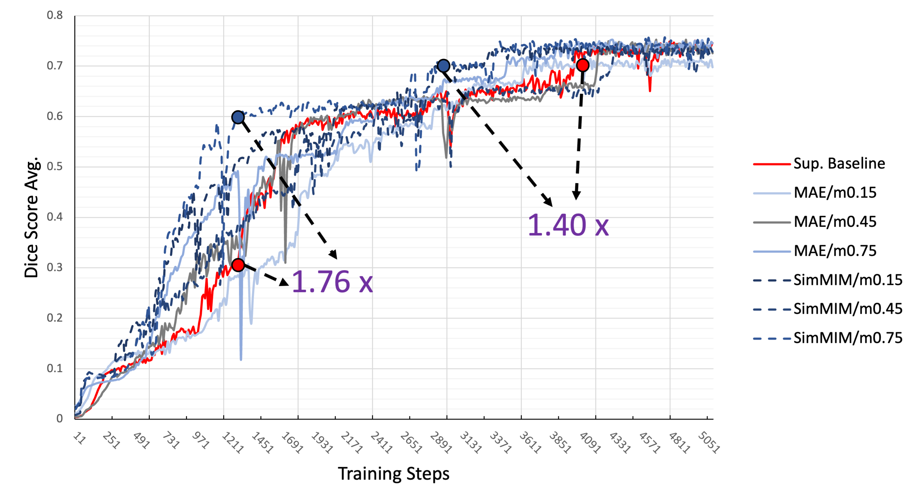
Recently, masked image modeling (MIM) has gained considerable attention due to its capacity to learn from vast amounts of unlabeled data and has been demonstrated to be effective on a wide variety of vision tasks involving natural images. Meanwhile, the potential of self-supervised learning in modeling 3D medical images is anticipated to be immense due to the high quantities of unlabeled images, and the expense and difficulty of quality labels. However, MIM’s applicability to medical images remains uncertain. In this paper, we demonstrate that masked image modeling approaches can also advance 3D medical images analysis in addition to natural images. We study how masked image modeling strategies leverage performance from the viewpoints of 3D medical image segmentation as a representative downstream task: i) when compared to naive contrastive learning, masked image modeling approaches accelerate the convergence of supervised training even faster (1.40) and ultimately produce a higher dice score; ii) predicting raw voxel values with a high masking ratio and a relatively smaller patch size is non-trivial self-supervised pretext-task for medical images modeling; iii) a lightweight decoder or projection head design for reconstruction is powerful for masked image modeling on 3D medical images which speeds up training and reduce cost; iv) finally, we also investigate the effectiveness of MIM methods under different practical scenarios where different image resolutions and labeled data ratios are applied.
1 Introduction
The demand for deep neural networks that conduct analysis tasks on 3D medical image data has expanded dramatically in recent years as a result of technological advances in deep learning and hardware compute capabilities. 3D medical volumetric images show a lot of potential in healthcare, where it can help increase the speed and accuracy of diagnosing patient conditions. For instance, properly and swiftly discovering and measuring tumor lesions from MRI/CT scans would be critical to disease prevention, early detection and treatment plan optimization, and would also spur the development of more successful clinical applications that would ultimately improve patients’ lives [6]. However, the high expense of expert annotation frequently stymies attempts to leverage advances in clinical outcomes using deep learning approaches. Annotations of 3D medical images at scale by radiologists are limited, expensive, and time-consuming to produce. Another barrier in 3D medical imaging is data volume, which is driven by the increased 3D image dimensionality and resolution, resulting in significant processing complexity. As a consequence, training deep learning models on 3D medical images from random initialization necessitates burdensome compute and data requirements.
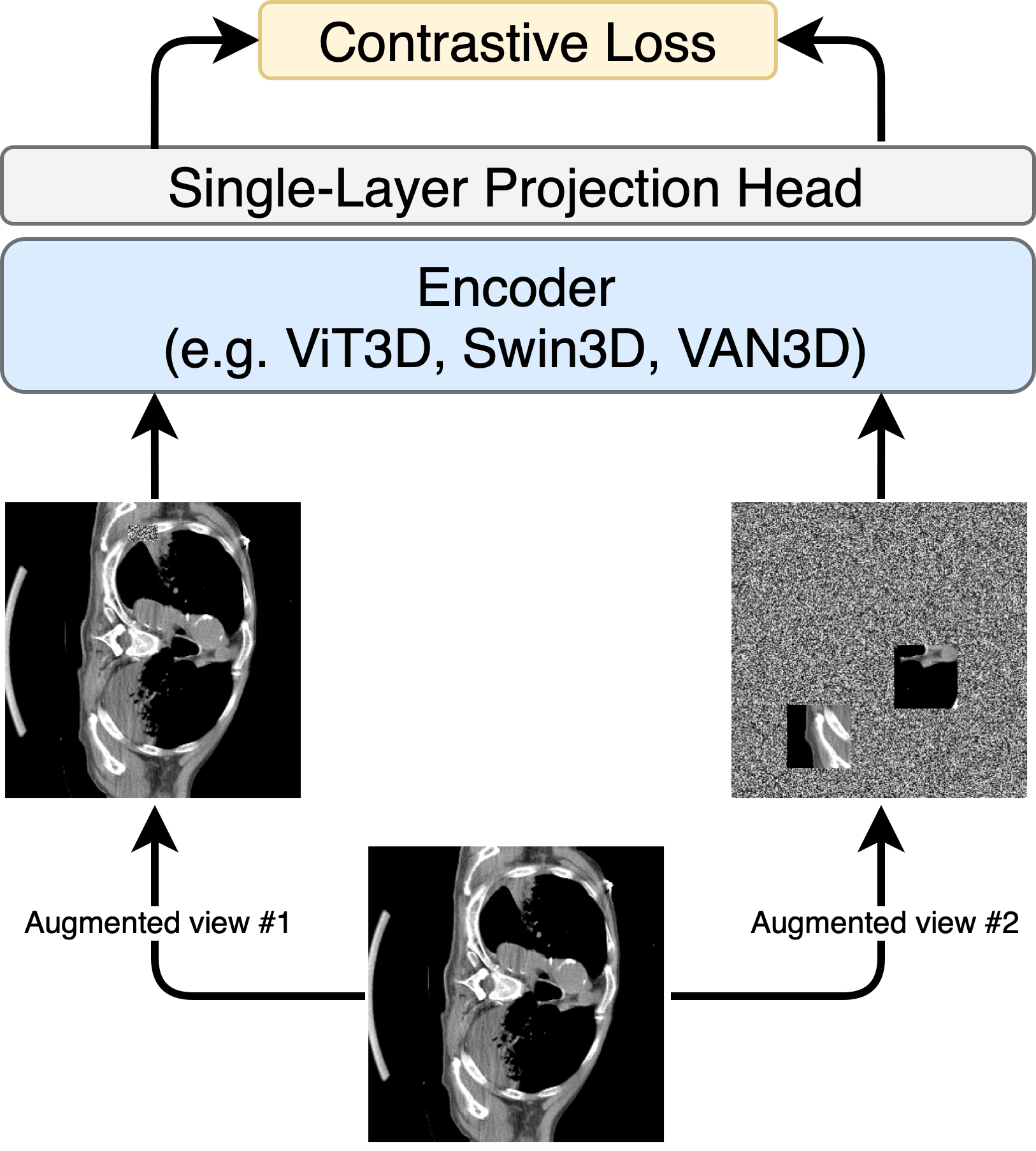
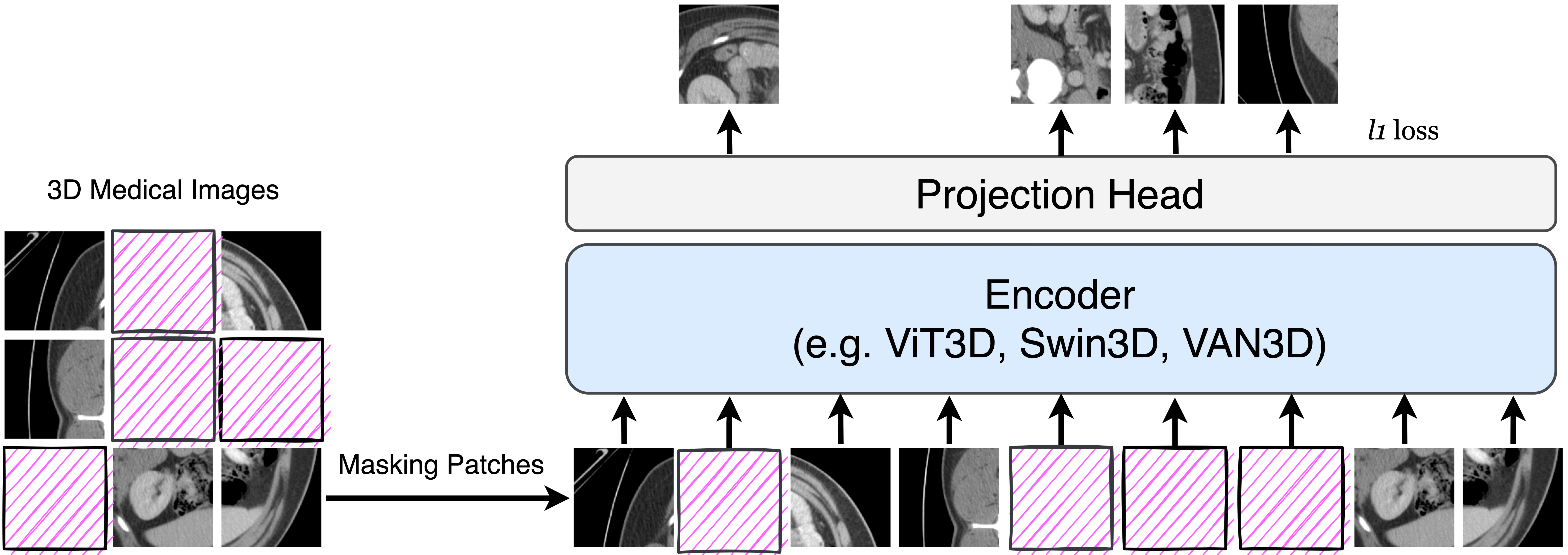
As a viable alternative, self-supervised learning [26] obtains supervisory signals from the data itself, and has recently been shown to successfully address the appetite for data and to be capable of learning generalizable dense representations of the input. Among contemporary approaches, masked signal modeling is one such learning task: masking a subset of input signals and attempting to forecast the masked signals. This paradigm has been extremely successful in NLP, since self-supervised learning algorithms based on the masked language modeling task have largely revolutionized the discipline [13, 39, 40, 7], demonstrating that giant models such as BERT [13] and GPT [39, 40, 7] can be learned on unlabeled text data and adapted to a wide variety of applications. More importantly, with the introduction of Vision Transformers (ViT) [50, 15], the architecture gap, where it was not intuitive to apply mask tokens[50, 13] using covolutions [27], is no longer an obstacle. Following this philosophy, latest approaches based on masked image modeling (MIM) have demonstrated their efficacy in the development of scalable vision models [23, 55, 2]. Despite these accomplishments, masked image modeling based algorithms have received little attention in medical imaging modeling, and their applicability has not been thoroughly investigated. Naturally, we wonder whether masked image modeling will advance 3D medical imaging analysis as well. In this work, we aim to address this question from the following attempts:
-
•
Contrastive learning [5, 19, 10] has been proven in a few studies to be capable of learning generic representations of medical images that leverage the downstream tasks such as 3D segmentation and classification [46, 1, 47]. It is worthwhile to compare masked image modeling to contrastive learning approaches (see Fig. 1(a) for illustration) on medical images.
-
•
Natural images are raw, low-level signals with a significant degree of spatial redundancy; restoring some missing patches can be accomplished by directly copying surrounding patches with little high-level understanding of the objects and sceneries [23]. Particularly for certain CT/MRI scans with solid tumors, the majority of background tissues are comparable, making it even more difficult for the model to learn useful features about the lesion regions. As a result, we assess several masking strategies (masked patch size and masking ratio) in order to determine the most efficient way that promotes holistic comprehension beyond low-level data while avoiding excessive attention to features such as texture and materials.
-
•
In practice, medical image analysis is utilized in a variety of contexts with varying amounts of annotated data, accessible unlabeled data, and even image resolutions. As a result, it is also vital for us to extensively analyze how these elements affect the pertaining as well as the performance on downstream tasks.
This paper investigates how masked image modeling based self-supervised learning can be utilized to improve 3D medical image analysis. It does so by conducting extensive experiments on two real-world benchmark datasets: multi-organ segmentation111https://www.synapse.org/#!Synapse:syn3193805/wiki/89480 and brain tumor segmentation [44]. Our experimental results demonstrate that masked image modeling is advantageous for modeling 3D medical images by significantly speeding up training convergence (e.g. at most 1.4 training cost saving to reach the same dice score) and ultimately improved downstream performance (e.g. over 5 improvements on both segmentation without any hyperparameter tuning).

2 Related Work
Transfer Learning in Medical Image Analysis.
Transfer learning from natural images is extensively utilized in medical image analysis [31, 34], regardless disparities in image statistics, scale, and task-relevant characteristics. Raghu et al. [41] and [1] showed that transfer learning from ImageNet can accelerate convergence on medical images, which is especially useful when the medical image training data is limited. Transfer learning using domain-specific data can also assist in resolving the domain disparity issue. For instance, [9, 29] indicate improved performance following pretraining on labeled data from the same domain. However, this strategy is frequently impractical for a variety of medical scenarios requiring labeled data that is costly and time-consuming to gather. Recent improvements in self-supervised learning offer a viable alternative, allowing for the utilization of unlabeled medical data, which is massive and commonly more accessible.
Masked Image Modeling.
Masked image modeling is a self-supervised learning method that learns representations via masking-corrupted images. It evolved in line with the MLM task in NLP but remained out of the mainstream for a long period. DAE [51] is a pioneering work in this domain, presenting masking as a noise type. The context encoder [37] predicts the missing pixels by inpainting a large rectangular area of the source images. Recent techniques [8, 15, 4] based on Transformers [50] are motivated by the success of NLP. iGPT [8] groups pixel values into different clusters and classify unknown pixels. The ViT study [15] investigates masked patch prediction for self-supervised learning by predicting the mean color of images. BEiT [4] recently used a dVAE network to tokenize and forecast pixel values into discrete numbers [49, 42]. More importantly, MAE [23] adheres the spirit of raw pixel restoration, demonstrating for the first time that masking a high proportion of the input images can yield a non-trivial and meaningful self-supervisory task. It adopts a design of autoencoder with a lightweight decoder, which reduces training costs even more. SimMIM [55] takes it a step further and substitutes the entire decoder with a single linear projection layer, resulting in comparable results. The very recent approaches such as data2vec [2] and CAE [11] make predictions in the latent representation space from the visible patches to the masked patches, attempting to make MIM a more universal framework for self-supervised learning. Nonetheless, the techniques described above have only been shown to be useful for natural images modeling. In this work, we aim to investigate whether MIM approaches can also advance 3D medical image analysis.
Self-Supervised Learning.
Early work in self-supervised learning focuses on learning representations from unlabeled data so that a low-capacity classifier can achieve high accuracy using these embeddings [14, 52, 35, 56, 36, 16]. For years, contrastive learning [5, 19, 53, 48, 24, 10] has received much interest as one of the most popular and widespread self-supervised learning strategies. It models image similarity and dissimilarity (or solely similarity [17, 12]) between two or more views, with data augmentation being crucial for contrastive and related approaches. Self-supervised learning has also been used in the medical field, according to several previous literature. Domain-specific pretext tasks [45, 3, 59, 58], for example, have been studied, while other work [30, 25, 57, 28] focuses on tailoring contrastive learning to medical data. Taleb et al. [46], in particular, examine a range of self-supervised learning strategies for 3D medical imaging in depth. MICLe [1] demonstrates that a model pretrained on ImageNet can also advance Dermatology image classification. Tang et al. [47] further combines inpainting [37] with contrastive learning for medical segmentation. Despite the fact that all of these methods have showed promise in medical imaging, masked image modeling-based methods have yet to be substantially investigated in this discipline.
3 Approach
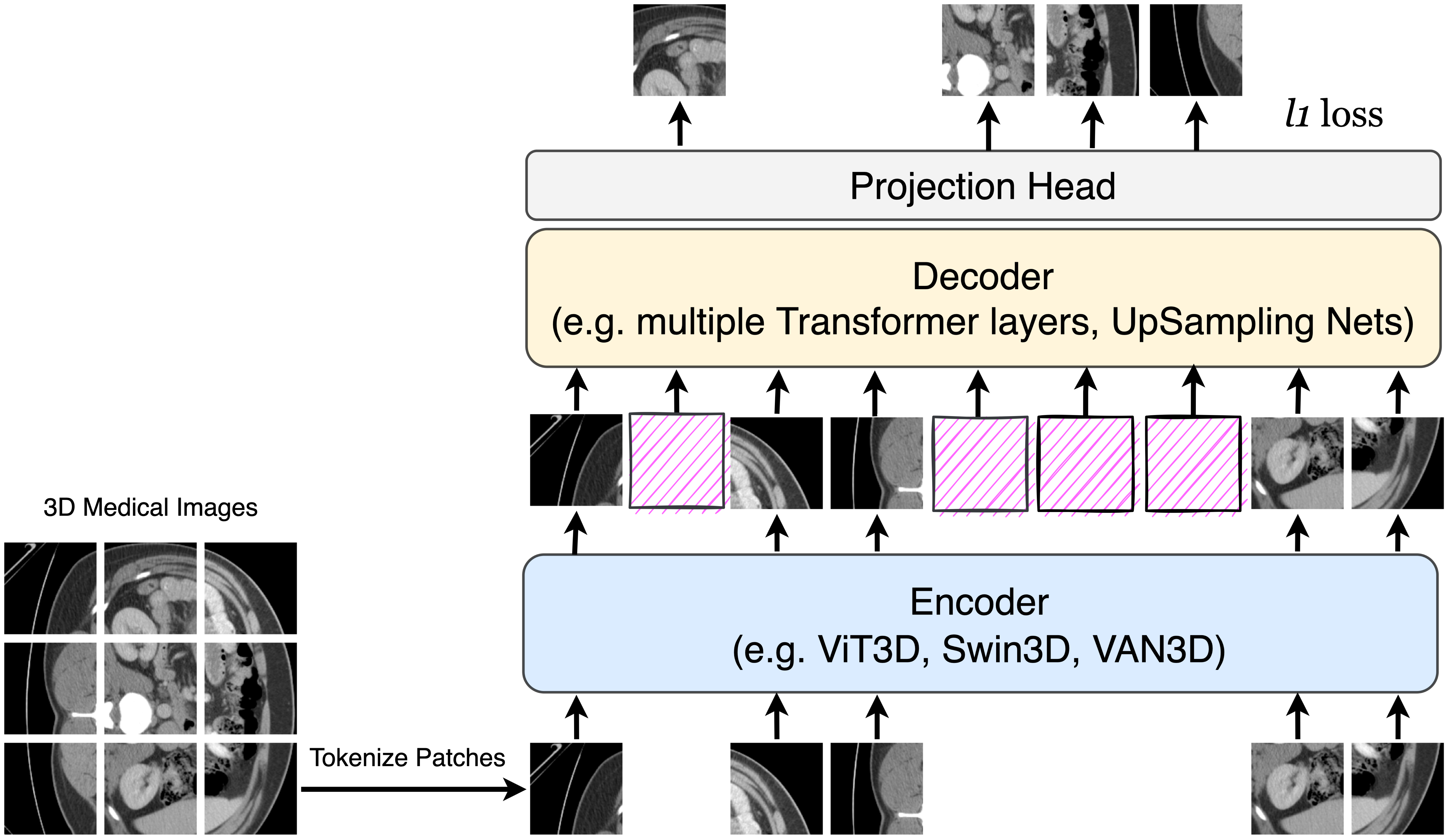
Masked image modeling approaches, in general, mask out a portion of input images or encoded image tokens and encourage the model to recreate the masked area. Many extant MIM models employ an encoder-decoder design followed by a projection head, such as BEiT [4] and MAE [23]. The encoder aids in the modeling of latent feature representations, while the decoder aids in the resampling of latent vectors to original images. The encoded or decoded embeddings will subsequently be aligned with the original signals at the masked area by a projection head. Notably, the decoder component has been suggested to be designed in a lightweight manner in order to minimize training time. A lightweight decoder, in our experience, not only reduces computing complexity but also increases the encoder’s ability to learn more generalizable representations that the decoder can easily grasp, translate and convey. As a result, while the encoder is more important (only encoder would be inherited for finetuning), methods like SimMIM [55] simplifies the architecture even more by obviating the entire decoder with a single projection layer. In this work, we thoroughly investigate the effectiveness of different MIM models on 3D medical imaging data. The following components provide more details:
3.1 Masking Strategies
Following ViT[15], an image is divided into regular non-overlapping patches (e.g. a 96 96 96 3D volume will be divided into 216 patches of 16 16 16 smaller volumes), which are often considered as the basic processing units of vision Transformers. Multiple random masking methods have been proposed in the previous literature: 1) InPainting [37] introduced a central region masking strategy; 2) BEiT [4] proposed a complex block-wise masking strategy; 3) most recent approaches such as MAE [23] and SimMIM [55] followed a more straightforward uniformly random masking method at patch-level while investigating different masked patch sizes and masking ratios (see Fig. 1(b) and Fig. 1(c), respectively). Many random masking schemes are also patch-based since it is more convenient to operate masking on a patch-by-patch basis, where a patch is either fully visible or masked. As demonstrated by these works, the uniformly random sampling with a high masking ratio effectively eliminates redundancy, resulting in a self-supervisory task that cannot be easily solved by extrapolation from visible neighboring patches. Meanwhile, a potential center bias (i.e. more masked patches near the image center) is avoided by the uniform distribution. Finally, the sparse input allows for the development of an efficient encoder, which will be discussed next. In this work, we also use the random patch masking approach for simplicity and efficacy.
3.2 Encoders
Encoders are responsible for modeling latent feature representations of the masked patches, which are then utilized to forecast the original signals in the masked area. The learned encoder should be capable of adapting to a wide range of vision tasks. We consider a variety of architectures in this paper, including two fundamental vision Transformer architectures: vanilla ViT [50, 15] and SwinTransformer [32], as well as one attentional visual network VAN [18], which inherits the attention mechanism to derive hierarchical representations similar to SwinTransformer but using pure convolutions. All models are reimplemented to 3D versions in order to accommodate the 3D volume data. We simply refer to these models as ViT3D, SwinTransformer3D and VAN3D.
3.3 Decoders
For methods that follow an auto-encoder design to reconstruct the image, the decoder takes the entire collection of encoded tokens, including 1) encoded visible patches and 2) mask tokens. Each randomly initialized mask token is a learnable vector that is jointly optimized to reveal the masked patches. The absolute positional embeddings [50] or relative positional embeddings [32] are also applied to these mask tokens corresponding to the backbone architecture. Additionally, all the masked patches are invisible to the encoder and only the decoder can see all tokens. As proved in [23], this can save more computation and memory while not interfering with training. Meanwhile, the decoder backbones are independent from the encoder backbones, which are likewise optional (see Fig. 1(b)). By default, we follow [23] and use another series of Transformer blocks for decoding.
3.4 Reconstruction Target
Raw voxel value prediction.
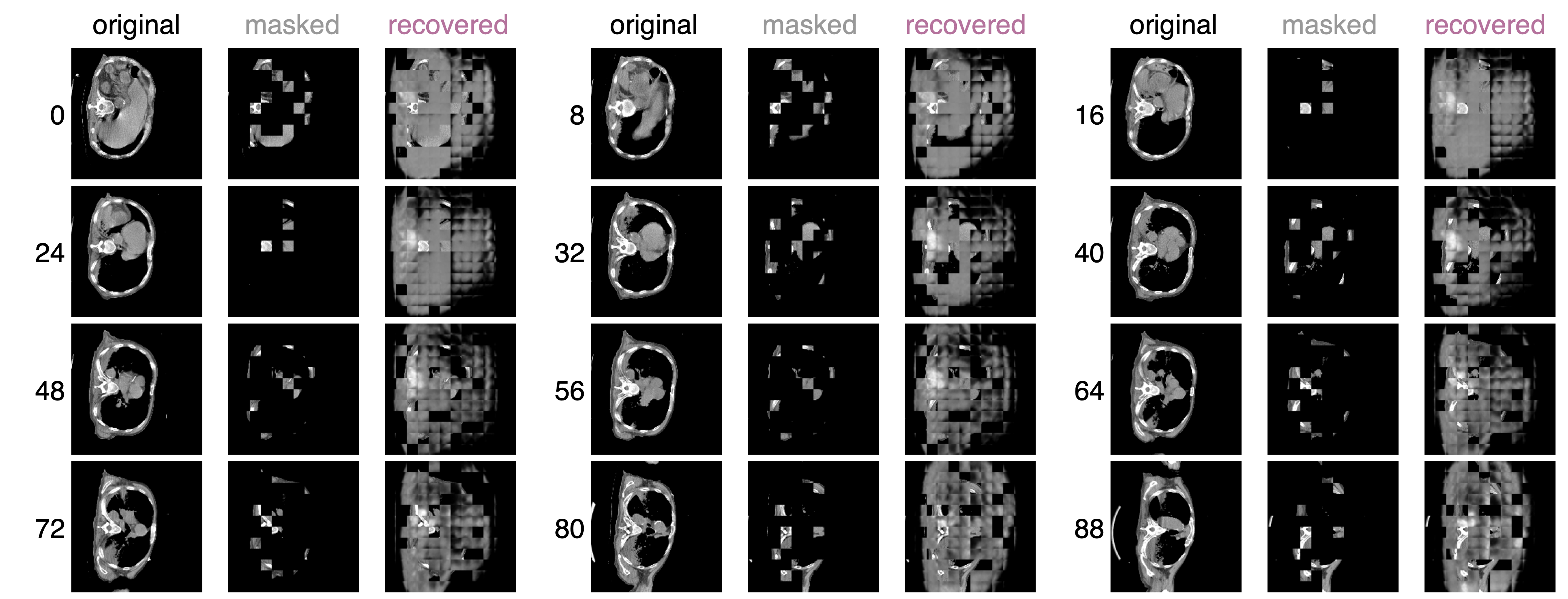
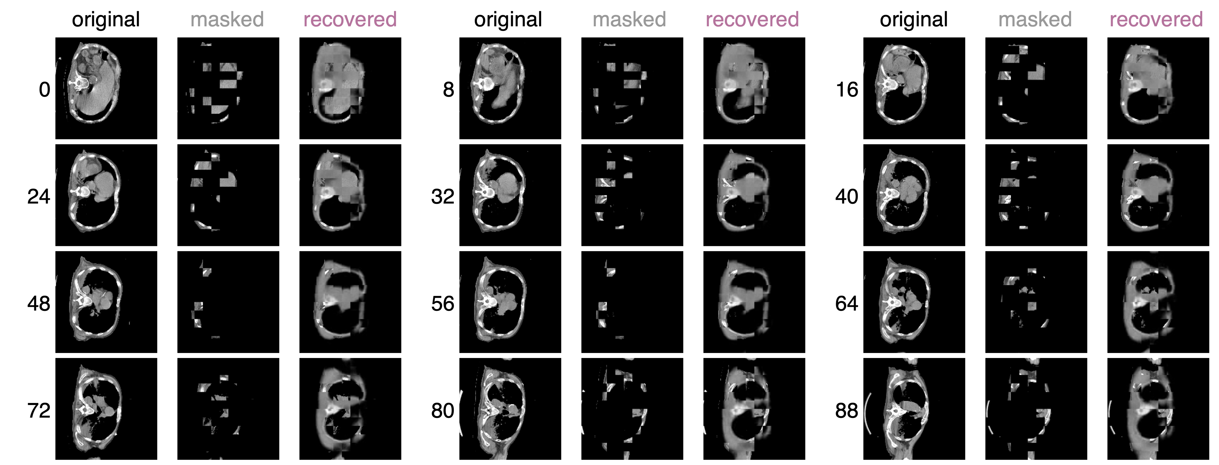
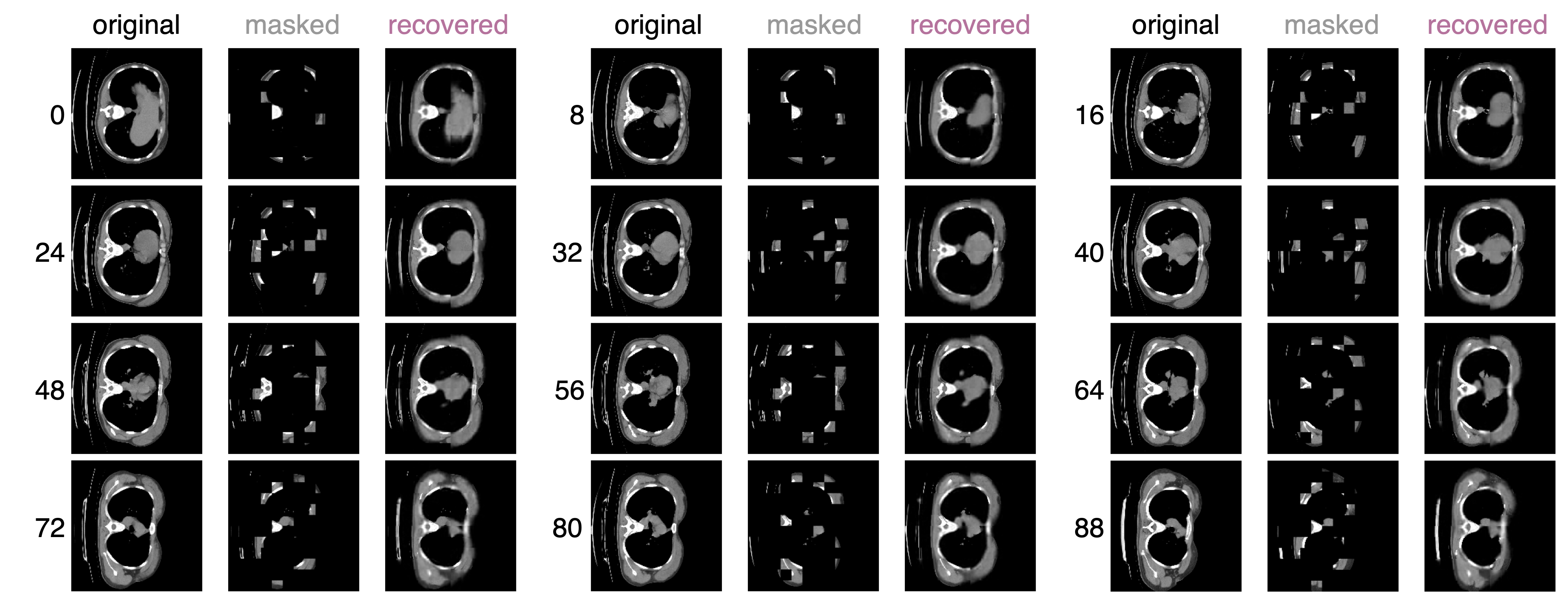
For 3D medical image, reconstructing the inputs by estimating the raw voxel values for each mask token is simple and intuitive. The distance between recovered and original images in voxel space can be computed using a loss function of either loss or loss. Furthermore, the loss is only computed on masked patches, preventing the model from engaging in self-reconstruction, which might potentially dominate the learning process and ultimately impede knowledge learning. Notably, most vision Transformer topologies will downsample the original image resolution. For 3D medical images, a 96 volume resolution will be downsampled to 9 (i.e. 1*9*9*9768 using ViT-Base) and 3 using SwinTransformer or VAN. Therefore, for vanilla ViT, we apply a single linear projection layer to transform the latent embeddings to the original voxel space; for SwinTransformer and VAN, we apply two-layers convolutional transpose to upsample the compressed embeddings to the original resolution. See Fig. 2 and Fig. 3 for the reconstruction of 3D lung CT scans from TCIA-COVID19 using SimMIM [55] and MAE [23], respectively.
Other predictions.
Many earlier studies transform masked signals to clusters or classes rather than raw pixel values. For example, iGPT [8] uses k-means to divide the RGB values into 512 clusters and encourage the model to predict which cluster each pixel belongs to. BEiT [4] employs a discrete VAE (dVAE) to convert image patches to discrete tokens. The prediction objective is then based on the token identity. Medical images, on the other hand, are often sparse, and voxel values are not scale intensive. The fine-grained texture or materials information may be lost by replacing the original signals with a discrete class target. As a result, we concentrate on predicting raw voxel values in this work for the sake of simplicity and robustness.
| Methods | Backbones | Multi-Organ Sementation | Avg. | ||||||||||||
|---|---|---|---|---|---|---|---|---|---|---|---|---|---|---|---|
| Spleen | RKid | LKid | Gall | Eso | Liv | Sto | Aor | IVC | Veins | Pan | RAG | LAG | |||
| Sup. baseline [22] our impl. | ViT3D-B [15] | 0.8902 | 0.8926 | 0.8769 | 0.4763 | 0.4891 | 0.9447 | 0.7475 | 0.8207 | 0.773 | 0.6175 | 0.6442 | 0.5663 | 0.4699 | 0.7084 |
| ViT3D-L | 0.8993 | 0.9018 | 0.8859 | 0.4813 | 0.4942 | 0.9543 | 0.7553 | 0.8292 | 0.7810 | 0.6239 | 0.6508 | 0.5721 | 0.4749 | 0.7157 | |
| Swin3D-T [32] | 0.8638 | 0.8661 | 0.8508 | 0.4622 | 0.4746 | 0.9166 | 0.7255 | 0.7963 | 0.7500 | 0.5992 | 0.6252 | 0.5496 | 0.4560 | 0.6874 | |
| Swin3D-S | 0.8792 | 0.8815 | 0.8661 | 0.4704 | 0.4831 | 0.9331 | 0.7383 | 0.8107 | 0.7635 | 0.6099 | 0.6363 | 0.5594 | 0.4641 | 0.6997 | |
| Swin3D-B | 0.8852 | 0.8876 | 0.8721 | 0.4737 | 0.4864 | 0.9395 | 0.7434 | 0.8162 | 0.7687 | 0.6141 | 0.6407 | 0.5632 | 0.4673 | 0.7045 | |
| VAN3D-S [18] | 0.8572 | 0.8595 | 0.8444 | 0.4587 | 0.4711 | 0.9098 | 0.7198 | 0.7904 | 0.7444 | 0.5946 | 0.6204 | 0.5454 | 0.4525 | 0.6822 | |
| VAN3D-B | 0.8813 | 0.8837 | 0.8682 | 0.4716 | 0.4843 | 0.9354 | 0.7401 | 0.8126 | 0.7653 | 0.6114 | 0.6379 | 0.5607 | 0.4653 | 0.7014 | |
| SimCLR [10] | ViT3D-B [15] | 0.9110 | 0.9135 | 0.8974 | 0.4875 | 0.5007 | 0.9669 | 0.7650 | 0.8399 | 0.7912 | 0.6320 | 0.6594 | 0.5795 | 0.4810 | 0.7249 |
| ViT3D-L | 0.9279 | 0.9304 | 0.9141 | 0.4965 | 0.5099 | 0.9849 | 0.7792 | 0.8556 | 0.8058 | 0.6437 | 0.6716 | 0.5904 | 0.4899 | 0.7385 | |
| MAE [23] | ViT3D-B [15] | 0.9488 | 0.9502 | 0.9341 | 0.5066 | 0.521 | 0.9863 | 0.7969 | 0.8742 | 0.8248 | 0.6589 | 0.6868 | 0.6052 | 0.5010 | 0.7534 |
| ViT3D-L | 0.9541 | 0.9566 | 0.9399 | 0.5105 | 0.5243 | 0.9878 | 0.8012 | 0.8797 | 0.8285 | 0.6618 | 0.6905 | 0.6070 | 0.5037 | 0.7574 | |
| SimMIM [55] | ViT3D-B [15] | 0.9520 | 0.9545 | 0.9378 | 0.5194 | 0.5232 | 0.9875 | 0.7995 | 0.8776 | 0.8267 | 0.6605 | 0.6890 | 0.6076 | 0.5126 | 0.7575 |
| ViT3D-L | 0.9556 | 0.9582 | 0.9414 | 0.5206 | 0.5352 | 0.9898 | 0.8025 | 0.8811 | 0.8298 | 0.6649 | 0.6916 | 0.6088 | 0.5045 | 0.7603 | |
| Swin3D-T [32] | 0.9157 | 0.9182 | 0.9021 | 0.4900 | 0.5032 | 0.9719 | 0.7690 | 0.8443 | 0.7952 | 0.6352 | 0.6628 | 0.5826 | 0.4834 | 0.7288 | |
| Swin3D-S | 0.9319 | 0.9344 | 0.9181 | 0.4987 | 0.5121 | 0.9891 | 0.7826 | 0.8593 | 0.8093 | 0.6465 | 0.6745 | 0.5929 | 0.4920 | 0.7416 | |
| Swin3D-B | 0.9387 | 0.9413 | 0.9248 | 0.5023 | 0.5159 | 0.9963 | 0.7883 | 0.8656 | 0.8152 | 0.6512 | 0.6794 | 0.5973 | 0.4956 | 0.7471 | |
| VAN3D-S [18] | 0.9090 | 0.9115 | 0.8955 | 0.4864 | 0.4995 | 0.9648 | 0.7634 | 0.8382 | 0.7894 | 0.6306 | 0.6579 | 0.5784 | 0.4799 | 0.7234 | |
| VAN3D-B | 0.9350 | 0.9375 | 0.9211 | 0.5003 | 0.5138 | 0.9924 | 0.7852 | 0.8621 | 0.8119 | 0.6486 | 0.6767 | 0.5949 | 0.4936 | 0.7441 | |
4 Experiments on 3D Segmentation
We evaluate masked image modeling methods on two separate 3D segmentation tasks that involve both CT and MRI imaging modalities.
BTCV/CT.
The BTCV dataset222https://www.synapse.org/#!Synapse:syn3193805/wiki/89480 comprises of 30 participants who had abdominal CT scans with 13 organs annotated by interpreters at Vanderbilt University Medical Center under the supervision of clinical radiologists. Each CT scan was performed in the portal venous phase with contrast enhancement and comprised of 80 to 225 slices with 512512 pixels and a slice thickness of 1 to 6 mm. Each volume was pre-processed separately, with intensities in the range of [-175, 200] HU being normalized to [0, 1]. During pre-processing, all images are resampled to 1.5/2.0 mm (different resolutions for ablation study) isotropic voxel spacing. The multi-organ segmentation problem is formulated as a 13 class segmentation task with 1-channel input. We use the first 24 volumes for training and report on 6 validation images.
BraTS/MRI.
Brain tumor segmentation is another important task. This BraTS dataset [44] contains a training set of 387 multi-modal multi-site MRI data (FLAIR, T1w, T1gd, T2w) with ground truth labels of gliomas segmentation necrotic/active tumor and edema is used for brain tumor segmentation. The voxel spacing of MRI images in this task is 1.01.01.0 mm3. The voxel intensities are pre-processed with z-score normalization. The problem of brain tumor segmentation is formulated as a 3 class segmentation task with 4-channel input. We report on 97 validation images.
TCIA-COVID19/CT.
This is a public dataset [20] consisting of unenhanced chest CTs of patients with COVID19 infections. There are 771 volumes collected from 661 patients in total. All images are unannotated. We utilize this dataset as an extra unlabeled dataset for self-supervised learning in ablation study. All models in Tab. 1 are pretrained using a combination of this dataset and BTCV. In ablation study, we also compare the performance between pretraining with and without this dataset.
Supervised Baselines.
UNETR [22] is a U-shaped encoder-decoder architecture for medical segmentation that employs a ViT as the encoder backbone and a convolutional upsampling decoder following U-Net [43] design. It is one of the SOTA models in the domain of medical imaging segmentation that incorporates the vision Transformers as the backbone. UNETR-Base represents a ViT-Base [15] is applied as the encoder backbone. We adopt UNETR-B as the default supervised baseline in our ablation study. For other backbones (SwinTransformer and VAN) that produce hierarchical features, we adopt UPerNet [54] as the decode head by default for downstream segmentation.
Evaluation Metric
We use the Dice score to evaluate the accuracy of segmentation in our experiments. For a given semantic class, let and denote the ground truth and prediction values for voxel . The Dice score is defined as:
| (1) |
Implementation Settings.
All of the models are implemented in PyTorch333https://pytorch.org. We use MONAI444https://github.com/Project-MONAI for data transformations and loading. In our ablation studies, we use ViT-Base [15] as the default encoder backbone. For supervised baseline of organ segmentation, we employ a batch size of 4, the AdamW [33] optimizer, and a learning rate of 0.0003 with a weight decay of 0.05 (because ViT based architectures are huge and easily overfit) based on a linear warmup up to 300 epochs and cosine annealing scheduler. Training is conducted on a single NVIDIA A10G instance for a total of 3000 epochs. For brain tumor segmentation, the batch size is set to 8 as the training is conducted on 4 NVIDIA A10G GPUs for a total number of 1000 epochs. We use a 100 epochs linear warmup and the optimizer settings are compatible with organ segmentation. Our Appendix provides additional information Sec. 6.
| Methods | Backbones | Brain Tumor Sementation | Avg. | ||
|---|---|---|---|---|---|
| TC | WT | ET | |||
| Sup. baseline [22] our impl. | ViT3D-B [15] | 0.8162 | 0.8781 | 0.5734 | 0.7559 |
| ViT3D-L | 0.8178 | 0.8798 | 0.5745 | 0.7574 | |
| SimCLR [10] | ViT3D-B [15] | 0.8360 | 0.8988 | 0.5869 | 0.7739 |
| ViT3D-L | 0.8313 | 0.8944 | 0.5842 | 0.7699 | |
| MAE [23] | ViT3D-B [15] | 0.8690 | 0.9340 | 0.6104 | 0.8045 |
| ViT3D-L | 0.8723 | 0.9385 | 0.6130 | 0.8079 | |
| SimMIM [55] | ViT3D-B [15] | 0.8734 | 0.9394 | 0.6103 | 0.8077 |
| ViT-L | 0.8738 | 0.9401 | 0.6141 | 0.8093 | |
| Swin3D-S [32] | 0.8428 | 0.9067 | 0.5922 | 0.7806 | |
| Swin3D-B | 0.8556 | 0.9205 | 0.6013 | 0.7924 | |
| VAN3D-B [18] | 0.8406 | 0.9043 | 0.5907 | 0.7785 | |
| VAN3D-L | 0.8522 | 0.9169 | 0.5989 | 0.7893 | |
4.1 Comparison among Different Approaches
We begin by evaluating 1) how masked image modeling methods compare to contrastive learning approaches and 2) how different masked image modeling approaches perform in comparison to one another using MAE [23] and SimMIM [55] and a conventional contrastive learning methodology SimCLR [10]. We evaluate a range of encoder backbones with varying network sizes, including pure vision Transformer [15], SwinTransformer [32], and visual attentional network (VAN) [18]. For MAE, we use an 8-layer Transformer block with 512-d as the decoder; for SimMIM, we use a single linear layer as the projection head. We use a two-layer convolutional transpose as the projection head for pretraining and the UPerNet [54] for segmentation in both Swin3D and VAN3D. All other hyper-parameters were set identically in this investigation. Additionally, because the full 3D image volume is typically difficult to load directly into the GPU (memory explosion), we employ a sliding window training strategy [38, 22, 21] in which the original image is divided into several (969696) small 3D windows. For all ViTs, a patch size of 16 is utilized by default.
Tab. 1 demonstrates that masked image modeling approaches outperform contrastive learning methods in general, as both MAE [23] and SimMIM [55] achieve an average dice score of around 0.7520.758, while SimCLR achieves an average dice score of around 0.723, which is 4.5 lower than the best approach. The segmentation findings for BraTS in Tab. 2 follow a similar pattern. The average dice score for masked image modeling approaches is somewhat greater than 0.80, however SimCLR [10] obtains a dice value of 0.7739, which is 4.37 lower than the best approach comparable to Tab. 1. Another note is that, despite the similarity of the two MIM techniques, SimMIM [55] achieves slightly better performance than MAE [23], as demonstrated by both Tab. 1 and Tab. 2. One explanation for this phenomena is because an efficient decoder (even a lightweight one) may be able to reconstruct the original image even if the encoder does not acquire generalizable representations, hence cyclically ease the motivation of encoder to learn more effective representations. Self-supervised learning’s ultimate goal is always to learn effective and generalizable representations of the data rather than self-convergence only. In comparison, SimMIM [55] employs an even lighter design by omitting the decoder entirely, which pushes the encoder to perform more complex reconstruction and learning tasks.
Additionally, masked image modeling approaches dramatically increase the training speed and reduce the cost, as seen by Fig. 4. SimMIM based architectures can obtain a 1.76 better dice score at the 1.3k training step. Moreover, MIM based approaches can reach a dice score of 0.7 with 1.4 less training time than the training time required for supervised baseline.
| Methods | Masked patch size | Masking ratio | Dice score Avg. |
|---|---|---|---|
| MAE [23] | 16 | 0.15 | 0.7156 |
| 16 | 0.30 | 0.7114 | |
| 16 | 0.45 | 0.6896 | |
| 16 | 0.60 | 0.7153 | |
| 16 | 0.75 | 0.7183 | |
| 24 | 0.15 | 0.6471 | |
| 24 | 0.45 | 0.7123 | |
| 24 | 0.75 | 0.7244 | |
| 32 | 0.15 | 0.7065 | |
| 32 | 0.45 | 0.7184 | |
| 32 | 0.75 | 0.7048 | |
| SimMIM [55] | 16 | 0.15 | 0.7144 |
| 16 | 0.30 | 0.7248 | |
| 16 | 0.45 | 0.7227 | |
| 16 | 0.60 | 0.7208 | |
| 16 | 0.75 | 0.7249 | |
| 24 | 0.15 | 0.7292 | |
| 24 | 0.45 | 0.7278 | |
| 24 | 0.75 | 0.7156 | |
| 32 | 0.15 | 0.7471 | |
| 32 | 0.45 | 0.7264 | |
| 32 | 0.75 | 0.7245 |
| Methods | Masked patch size | Masking ratio | Dice score Avg. |
|---|---|---|---|
| MAE [23] | 16 | 0.15 | 0.7864 |
| 16 | 0.30 | 0.7854 | |
| 16 | 0.45 | 0.7902 | |
| 16 | 0.60 | 0.7965 | |
| 16 | 0.75 | 0.8045 | |
| 24 | 0.15 | 0.7412 | |
| 24 | 0.45 | 0.7947 | |
| 24 | 0.75 | 0.8041 | |
| 32 | 0.15 | 0.7823 | |
| 32 | 0.45 | 0.7819 | |
| 32 | 0.75 | 0.8041 | |
| SimMIM [55] | 16 | 0.15 | 0.7818 |
| 16 | 0.30 | 0.7923 | |
| 16 | 0.45 | 0.7945 | |
| 16 | 0.60 | 0.8058 | |
| 16 | 0.75 | 0.8077 | |
| 24 | 0.15 | 0.7852 | |
| 24 | 0.45 | 0.7654 | |
| 24 | 0.75 | 0.7982 | |
| 32 | 0.15 | 0.7985 | |
| 32 | 0.45 | 0.7958 | |
| 32 | 0.75 | 0.7986 |
|
Pretrain data | Labeled ratio | Dice avg. | ||
|---|---|---|---|---|---|
| (2.0x, 2.0x, 2.0x) | COVID19 + BTCV | 0.6919 | |||
| (2.0x, 2.0x, 2.0x) | COVID19 + BTCV | 0.7338 | |||
| (1.5x, 1.5x, 2.0x) | COVID19 + BTCV | 0.7024 | |||
| (1.5x, 1.5x, 2.0x) | COVID19 + BTCV | 0.7534 | |||
| (2.0x, 2.0x, 2.0x) | BTCV | 0.6552 | |||
| (2.0x, 2.0x, 2.0x) | BTCV | 0.7018 | |||
| (1.5x, 1.5x, 2.0x) | BTCV | 0.6814 | |||
| (1.5x, 1.5x, 2.0x) | BTCV | 0.7183 |
4.2 Masking Strategy
Additionally, we investigate the effectiveness of different masked patch sizes and masking ratios on self-supervised learning performance. The performance of several MIM techniques at finetuning segmentation is summarized in Tab. 3 and Tab. 4. The following observations are made: i) Consistent with the original MAE literature [23], we conclude that a higher masking ratio is a non-trivial self-supervised learning job that would continually drive the model to build generalizable representations that can be transferred effectively to downstream tasks. For example, the best dice scores on multi-organ segmentation and brain tumor segmentation tasks are obtained when a masking ratio of 0.75 is used across multiple patch sizes (e.g., 0.7183 for patch size 16 in Tab. 3, and 0.8041 for patch sizes 24 and 32 in Tab. 4). ii) A high masking ratio combined with a small patch size likewise results in a relatively good performance when used in conjunction with SimMIM [55], similar to MAE [23]. As demonstrated by Tab. 3 and Tab. 4, when the patch size is equal to 16, the models perform optimally with dice scores of 0.7249 and 0.8077, respectively. iii) However, as the patch size increases, the SimMIM [55] method appears to be less sensitive to this masking ratio. For instance, when the patch size is 32, models can earn the highest dice score with a masking ratio of 0.15, the smallest possible masking ratio. One hypothesis is that medical images are typically raw, low-level signals with a large degree of spatial redundancy; recovering some missing patches can be performed by directly copying nearby patches with little comprehensive knowledge of the objects and surroundings. A single small masked patch is incapable of adequately masking complicated and intersecting structures or locations, but a high patch size may be able to hide more significant signals independently. As a result, a high masking ratio for small patch sizes is more critical than a high masking ratio for big patch sizes.
4.3 Data vs. Resolutions vs. Labeled Ratio
In this section, we analyze the results to address the following three questions: i) Does increasing the amount of pretraining data improve downstream performance? ii) How do different pretrained resolutions affect downstream knowledge transfer? And iii) how do masked image learning approaches improve performance when using varying amounts of labeled data? All pretraining in Tab. 5 is based on the MAE [23] architecture, which utilizes a ViT-Base/16 as the backbone with a masking ratio of 75, as demonstrated in Tab. 3 and Tab. 4. Differently labeled ratios indicate that we employ a varying percentage of annotated BTCV CT scans (e.g., 50 = 12 images, 100 = 24 images) for downstream finetuning, whereas the validation set of 6 images is consistent.
In the majority of supervised learning cases, more training data results in improved performance. Given that the majority of medical images are similar from the bottom logic up, we ask if this holds true in the case of self-supervised learning, and in particular, how much benefits can be gained through size of pretrain data when utilizing MIM for 3D medical analysis. We adopt multi-organ segmentation as the example downstream task and create two distinct training scenarios: one that uses both COVID19 and BTCV datasets and another that uses only BTCV. Tab. 5 demonstrates the constant tendency that models trained on more plentiful pretrained data outperform models trained on less pretrained data (e.g., 0.75340.7183: 4.9 improvements, 0.73380.7018: 4.6 improvements). This advantage is even more pronounced at lower image resolutions, as 0.6919 is 5.6 more than 0.6552 when only half labeled data is used.
In Tab. 5, we also explore how different pretrained image resolutions affect the downstream task performance. Intuitively, a higher pretraining resolution should result in a better segmentation results [1], as the images contain more granular information. Here, we utilize different downsampled ratios to represent the degree to which the original signals are compressed in all dimensions for each volume. Specifically, a bilinear interpolation function is used in conjunction with MONAI’s555https://github.com/Project-MONAI spacingd transformations. As can be observed from Tab. 5, pretrained models with higher resolutions (1.5x, 1.5x, 2.0x) generally perform better than pretrained models with lower resolutions (2.0x, 2.0x, 2.0x). For instance, 0.7338 dice score is 2.7 lower than the one pretrained using the same data source and labeled ratio but using a greater resolution.
In practical situation, the majority of the medical images, such as CT/MRI scans, are left unannotated due to the high cost of labeling. However, the public data is freely available and abundant, the aforementioned results illustrate once again that pre-training on large datasets followed by fine-tuning with small samples is feasible. It also demonstrates that masked image learning can significantly improve the downstream task performance in a variety of contexts.
5 Conclusion
This paper demonstrates how masked image modeling approaches in self-supervised learning leverage 3D medical image modeling by conducting extensive experiments on two sample segmentation tasks. We show how masked image modeling outperforms traditional contrastive learning by speeding up convergence and greatly improving downstream task performance. We also show how masked image modeling approaches can be utilized to advance 3D medical image modeling in a variety of situations. However, the fact that almost all medical images are weakly labeled (e.g. as little as few lines of text for description) rather than entirely unannotated is an open question we would like to investigate further in the future. We are then interested on comparing self-supervised learning to supervised learning with limited supervisory signals. Finally, we remain curious to see how self-supervised learning is integrated in other more challenging downstream tasks.
References
- [1] Shekoofeh Azizi, Basil Mustafa, Fiona Ryan, Zach Beaver, Jana von Freyberg, Jonathan Deaton, Aaron Loh, Alan Karthikesalingam, Simon Kornblith, Ting Chen, Vivek Natarajan, and Mohammad Norouzi. Big self-supervised models advance medical image classification. ICCV, 2021.
- [2] Alexei Baevski, Wei-Ning Hsu, Qiantong Xu, Arun Babu, Jiatao Gu, and Michael Auli. data2vec: A general framework for self-supervised learning in speech, vision and language. ArXiv, abs/2202.03555, 2022.
- [3] Wenjia Bai, Chen Chen, Giacomo Tarroni, Jinming Duan, Florian Guitton, Steffen Erhard Petersen, Yike Guo, Paul M. Matthews, and Daniel Rueckert. Self-supervised learning for cardiac mr image segmentation by anatomical position prediction. MICCAI, 2019.
- [4] Hangbo Bao, Li Dong, and Furu Wei. Beit: Bert pre-training of image transformers. ICLR, 2022.
- [5] Suzanna Becker and Geoffrey E. Hinton. Self-organizing neural network that discovers surfaces in random-dot stereograms. Nature, 355:161–163, 1992.
- [6] Kaustav Bera, Nathaniel Braman, Amit Gupta, Vamsidhar Velcheti, and Anant Madabhushi. Predicting cancer outcomes with radiomics and artificial intelligence in radiology. Nature Reviews Clinical Oncology, 19:132–146, 2021.
- [7] Tom B. Brown, Benjamin Mann, Nick Ryder, Melanie Subbiah, Jared Kaplan, Prafulla Dhariwal, Arvind Neelakantan, Pranav Shyam, Girish Sastry, Amanda Askell, Sandhini Agarwal, Ariel Herbert-Voss, Gretchen Krueger, Tom Henighan, Rewon Child, Aditya Ramesh, Daniel M. Ziegler, Jeffrey Wu, Clemens Winter, Christopher Hesse, Mark Chen, Eric Sigler, Mateusz Litwin, Scott Gray, Benjamin Chess, Jack Clark, Christopher Berner, Sam McCandlish, Alec Radford, Ilya Sutskever, and Dario Amodei. Language models are few-shot learners. In NeurIPS, 2020.
- [8] Mark Chen, Alec Radford, Jeff Wu, Heewoo Jun, Prafulla Dhariwal, David Luan, and Ilya Sutskever. Generative pretraining from pixels. In ICML, 2020.
- [9] Sihong Chen, Kai Ma, and Yefeng Zheng. Med3d: Transfer learning for 3d medical image analysis. ArXiv, abs/1904.00625, 2019.
- [10] Ting Chen, Simon Kornblith, Mohammad Norouzi, and Geoffrey E. Hinton. A simple framework for contrastive learning of visual representations. ICML, 2020.
- [11] Xiaokang Chen, Mingyu Ding, Xiaodi Wang, Ying Xin, Shentong Mo, Yunhao Wang, Shumin Han, Ping Luo, Gang Zeng, and Jingdong Wang. Context autoencoder for self-supervised representation learning. ArXiv, abs/2202.03026, 2022.
- [12] Xinlei Chen and Kaiming He. Exploring simple siamese representation learning. CVPR, 2021.
- [13] Jacob Devlin, Ming-Wei Chang, Kenton Lee, and Kristina Toutanova. Bert: Pre-training of deep bidirectional transformers for language understanding. In NAACL, 2019.
- [14] Carl Doersch, Abhinav Kumar Gupta, and Alexei A. Efros. Unsupervised visual representation learning by context prediction. ICCV, 2015.
- [15] Alexey Dosovitskiy, Lucas Beyer, Alexander Kolesnikov, Dirk Weissenborn, Xiaohua Zhai, Thomas Unterthiner, Mostafa Dehghani, Matthias Minderer, Georg Heigold, Sylvain Gelly, Jakob Uszkoreit, and Neil Houlsby. An image is worth 16x16 words: Transformers for image recognition at scale. ICLR, 2021.
- [16] Spyros Gidaris, Praveer Singh, and Nikos Komodakis. Unsupervised representation learning by predicting image rotations. ICLR, 2018.
- [17] Jean-Bastien Grill, Florian Strub, Florent Altch’e, Corentin Tallec, Pierre H. Richemond, Elena Buchatskaya, Carl Doersch, Bernardo Ávila Pires, Zhaohan Daniel Guo, Mohammad Gheshlaghi Azar, Bilal Piot, Koray Kavukcuoglu, Rémi Munos, and Michal Valko. Bootstrap your own latent: A new approach to self-supervised learning. NeurIPS, 2020.
- [18] Meng-Hao Guo, Chengrou Lu, Zheng-Ning Liu, Ming-Ming Cheng, and Shiyong Hu. Visual attention network. ArXiv, abs/2202.09741, 2022.
- [19] Raia Hadsell, Sumit Chopra, and Yann LeCun. Dimensionality reduction by learning an invariant mapping. CVPR, 2006.
- [20] Stephanie A. Harmon, Thomas Sanford, Sheng Xu, Evrim B Turkbey, Holger R. Roth, Ziyue Xu, Dong Yang, Andriy Myronenko, Victoria L. Anderson, Amel Amalou, Maxime Blain, Michael T Kassin, Dilara Long, Nicole Varble, Stephanie M. Walker, Ulas Bagci, Anna Maria Ierardi, Elvira Stellato, Guido Giovanni Plensich, Giuseppe Franceschelli, Cristiano Girlando, Giovanni Irmici, Dominic LaBella, Dima A. Hammoud, Ashkan A. Malayeri, Elizabeth C. Jones, Ronald M. Summers, Peter L. Choyke, Daguang Xu, Mona G. Flores, Kaku Tamura, Hirofumi Obinata, Hitoshi Mori, F. Patella, Maurizio Cariati, Gianpaolo Carrafiello, Peng An, Bradford J. Wood, and Baris Turkbey. Artificial intelligence for the detection of covid-19 pneumonia on chest ct using multinational datasets. Nature Communications, 11, 2020.
- [21] Alireza Hatamizadeh, V. Nath, Yucheng Tang, Dong Yang, Holger R. Roth, and Daguang Xu. Swin unetr: Swin transformers for semantic segmentation of brain tumors in mri images. 2022.
- [22] Ali Hatamizadeh, Dong Yang, Holger R. Roth, and Daguang Xu. Unetr: Transformers for 3d medical image segmentation. WACV, 2022.
- [23] Kaiming He, Xinlei Chen, Saining Xie, Yanghao Li, Piotr Doll’ar, and Ross B. Girshick. Masked autoencoders are scalable vision learners. ArXiv, abs/2111.06377, 2021.
- [24] Kaiming He, Haoqi Fan, Yuxin Wu, Saining Xie, and Ross B. Girshick. Momentum contrast for unsupervised visual representation learning. CVPR, 2020.
- [25] X. He, Xingyi Yang, S. Zhang, J. Zhao, Y. Zhang, Eric P. Xing, and P. Xie. Sample-efficient deep learning for covid-19 diagnosis based on ct scans. medRxiv, 2020.
- [26] Ashish Jaiswal, Ashwin Ramesh Babu, Mohammad Zaki Zadeh, Debapriya Banerjee, and Fillia Makedon. A survey on contrastive self-supervised learning. ArXiv, abs/2011.00362, 2020.
- [27] Yann LeCun, Bernhard E. Boser, John S. Denker, Donnie Henderson, Richard E. Howard, Wayne E. Hubbard, and Lawrence D. Jackel. Backpropagation applied to handwritten zip code recognition. Neural Computation, 1:541–551, 1989.
- [28] Hongwei Li, Fei-Fei Xue, Krishna Chaitanya, Shengda Liu, Ivan Ezhov, Benedikt Wiestler, Jianguo Zhang, and Bjoern H. Menze. Imbalance-aware self-supervised learning for 3d radiomic representations. In MICCAI, 2021.
- [29] Gaobo Liang and Lixin Zheng. A transfer learning method with deep residual network for pediatric pneumonia diagnosis. Computer methods and programs in biomedicine, 2020.
- [30] Jingyun Liu, Gangming Zhao, Yue Fei, Ming Zhang, Yizhou Wang, and Yizhou Yu. Align, attend and locate: Chest x-ray diagnosis via contrast induced attention network with limited supervision. ICCV, 2019.
- [31] Yuan Liu, Ayush Jain, C. Eng, David Way, Kang Lee, Peggy Bui, Kimberly Kanada, Guilherme de Oliveira Marinho, Jessica Gallegos, Sara Gabriele, Vishakha Gupta, Nalini M. Singh, Vivek Natarajan, Rainer Hofmann-Wellenhof, Greg S Corrado, Lily H. Peng, Dale R. Webster, Dennis Ai, Susan J. Huang, Yun Liu, R. Carter Dunn, and David Coz. A deep learning system for differential diagnosis of skin diseases. Nature Medicine, 26:900–908, 2020.
- [32] Ze Liu, Yutong Lin, Yue Cao, Han Hu, Yixuan Wei, Zheng Zhang, Stephen Lin, and Baining Guo. Swin transformer: Hierarchical vision transformer using shifted windows. ICCV, 2021.
- [33] Ilya Loshchilov and Frank Hutter. Decoupled weight decay regularization. In ICLR, 2019.
- [34] Scott Mayer McKinney, Marcin Sieniek, Varun Godbole, Jonathan Godwin, Natasha Antropova, Hutan Ashrafian, Trevor Back, Mary Chesus, Greg Corrado, Ara Darzi, Mozziyar Etemadi, Florencia Garcia-Vicente, Fiona J. Gilbert, Mark D. Halling-Brown, Demis Hassabis, Sunny Jansen, Alan Karthikesalingam, Christopher J. Kelly, Dominic King, Joseph R. Ledsam, David S. Melnick, Hormuz Mostofi, Lily H. Peng, Joshua Jay Reicher, Bernardino Romera-Paredes, Richard Sidebottom, Mustafa Suleyman, Daniel Tse, Kenneth C. Young, Jeffrey De Fauw, and Shravya Shetty. International evaluation of an ai system for breast cancer screening. Nature, 577:89–94, 2020.
- [35] Mehdi Noroozi and Paolo Favaro. Unsupervised learning of visual representations by solving jigsaw puzzles. In ECCV, 2016.
- [36] Deepak Pathak, Ross B. Girshick, Piotr Dollár, Trevor Darrell, and Bharath Hariharan. Learning features by watching objects move. CVPR, 2017.
- [37] Deepak Pathak, Philipp Krähenbühl, Jeff Donahue, Trevor Darrell, and Alexei A. Efros. Context encoders: Feature learning by inpainting. CVPR, 2016.
- [38] H.T.R. Peiris, Munawar Hayat, Zhaolin Chen, Gary Egan, and Mehrtash Harandi. A volumetric transformer for accurate 3d tumor segmentation. ArXiv, abs/2111.13300, 2021.
- [39] Alec Radford and Karthik Narasimhan. Improving language understanding by generative pre-training. 2018.
- [40] Alec Radford, Jeffrey Wu, Rewon Child, David Luan, Dario Amodei, and Ilya Sutskever. Language models are unsupervised multitask learners. 2019.
- [41] Maithra Raghu, Chiyuan Zhang, Jon M. Kleinberg, and Samy Bengio. Transfusion: Understanding transfer learning for medical imaging. In NeurIPS, 2019.
- [42] Aditya Ramesh, Mikhail Pavlov, Gabriel Goh, Scott Gray, Chelsea Voss, Alec Radford, Mark Chen, and Ilya Sutskever. Zero-shot text-to-image generation. ICML, 2021.
- [43] Olaf Ronneberger, Philipp Fischer, and Thomas Brox. U-net: Convolutional networks for biomedical image segmentation. In MICCAI, 2015.
- [44] Amber L. Simpson, Michela Antonelli, Spyridon Bakas, Michel Bilello, Keyvan Farahani, Bram van Ginneken, Annette Kopp-Schneider, Bennett A. Landman, Geert J. S. Litjens, Bjoern H. Menze, Olaf Ronneberger, Ronald M. Summers, Patrick Bilic, Patrick Ferdinand Christ, Richard Kinh Gian Do, Marc J. Gollub, Jennifer Golia-Pernicka, Stephan Heckers, William R. Jarnagin, Maureen McHugo, Sandy Napel, Eugene Vorontsov, Lena Maier-Hein, and M. Jorge Cardoso. A large annotated medical image dataset for the development and evaluation of segmentation algorithms. ArXiv, abs/1902.09063, 2019.
- [45] Hannah Spitzer, Kai Kiwitz, Katrin Amunts, Stefan Harmeling, and Timo Dickscheid. Improving cytoarchitectonic segmentation of human brain areas with self-supervised siamese networks. In MICCAI, 2018.
- [46] Aiham Taleb, Winfried Loetzsch, Noel Danz, Julius Severin, thomas. gaertner, Benjamin Bergner, and C. Lippert. 3d self-supervised methods for medical imaging. NeurIPS, 2020.
- [47] Yucheng Tang, Dong Yang, Wenqi Li, Holger R. Roth, Bennett A. Landman, Daguang Xu, V. Nath, and Ali Hatamizadeh. Self-supervised pre-training of swin transformers for 3d medical image analysis. ArXiv, abs/2111.14791, 2021.
- [48] Aäron van den Oord, Yazhe Li, and Oriol Vinyals. Representation learning with contrastive predictive coding. ArXiv, abs/1807.03748, 2018.
- [49] Aäron van den Oord, Oriol Vinyals, and Koray Kavukcuoglu. Neural discrete representation learning. In NeurIPS, 2017.
- [50] Ashish Vaswani, Noam M. Shazeer, Niki Parmar, Jakob Uszkoreit, Llion Jones, Aidan N. Gomez, Lukasz Kaiser, and Illia Polosukhin. Attention is all you need. NeurIPS, 2017.
- [51] Pascal Vincent, H. Larochelle, Isabelle Lajoie, Yoshua Bengio, and Pierre-Antoine Manzagol. Stacked denoising autoencoders: Learning useful representations in a deep network with a local denoising criterion. J. Mach. Learn. Res., 11:3371–3408, 2010.
- [52] X. Wang and Abhinav Kumar Gupta. Unsupervised learning of visual representations using videos. ICCV, 2015.
- [53] Zhirong Wu, Yuanjun Xiong, Stella X. Yu, and Dahua Lin. Unsupervised feature learning via non-parametric instance discrimination. CVPR, 2018.
- [54] Tete Xiao, Yingcheng Liu, Bolei Zhou, Yuning Jiang, and Jian Sun. Unified perceptual parsing for scene understanding. In ECCV, 2018.
- [55] Zhenda Xie, Zheng Zhang, Yue Cao, Yutong Lin, Jianmin Bao, Zhuliang Yao, Qi Dai, and Han Hu. Simmim: A simple framework for masked image modeling. ArXiv, abs/2111.09886, 2021.
- [56] Richard Zhang, Phillip Isola, and Alexei A. Efros. Colorful image colorization. In ECCV, 2016.
- [57] Hong-Yu Zhou, Shuang Yu, Cheng Bian, Yifan Hu, Kai Ma, and Yefeng Zheng. Comparing to learn: Surpassing imagenet pretraining on radiographs by comparing image representations. In MICCAI, 2020.
- [58] Jiuwen Zhu, Yuexiang Li, Yifan Hu, Kai Ma, S. Kevin Zhou, and Yefeng Zheng. Rubik’s cube+: A self-supervised feature learning framework for 3d medical image analysis. Medical image analysis, 64:101746, 2020.
- [59] Xinrui Zhuang, Yuexiang Li, Yifan Hu, Kai Ma, Yujiu Yang, and Yefeng Zheng. Self-supervised feature learning for 3d medical images by playing a rubik’s cube. MICCAI, 2019.
6 Appendix
6.1 Experimental Settings
| config | value |
|---|---|
| optimizer | AdamW[33] |
| base learning rate | 3e-4 |
| weight decay | 0.005 |
| optimizer momentum | beta1, beta2 = 0.9, 0.999 |
| batch size | 4 |
| learning rate schedule | linear warmup cosine annealing |
| warmup epochs | 300 |
| total epochs | 3000 |
| augmentation | RangeScaleIntensity |
| config | value |
|---|---|
| optimizer | AdamW[33] |
| base learning rate | 3e-4 |
| weight decay | 0.005 |
| optimizer momentum | beta1, beta2 = 0.9, 0.999 |
| batch size | 2 |
| learning rate schedule | linear warmup cosine annealing |
| warmup epochs | 100 |
| total epochs | 1000 |
| augmentation | NormalizedIntensity |
| config | value |
|---|---|
| optimizer | AdamW[33] |
| base learning rate | 3e-4 |
| weight decay | 0.005 |
| optimizer momentum | beta1, beta2 = 0.9, 0.999 |
| batch size | 4 |
| learning rate schedule | linear warmup cosine annealing |
| warmup epochs | 300 |
| total epochs | 3000 |
| augmentation | RangeScaleIntensity |
| config | value |
|---|---|
| optimizer | AdamW[33] |
| base learning rate | 3e-4 |
| weight decay | 0.005 |
| optimizer momentum | beta1, beta2 = 0.9, 0.999 |
| batch size | 2 |
| learning rate schedule | linear warmup cosine annealing |
| warmup epochs | 100 |
| total epochs | 1000 |
| augmentation | RangeScaleIntensity |
As can be seen from the reconstructed volumes, the large model has more restoration power than the tiny model, which supports the previous conclusion. The flattened dimensionality of 3D medical images is frequently very high, and a small model would unavoidably compress the original voxel space into a smaller voxel space, thereby losing a lot of information.
