Online multiscale model reduction for nonlinear stochastic PDEs with multiplicative noise thanks: L.Jiang acknowledges the support of NSFC 11871378, the Fundamental Research Funds for the Central Universities and the support by Shanghai Science and Technology Committee 20JC1413500.

Lijian Jiang1 School of Mathematical Sciences, Tongji University, Shanghai 200092, China. (ljjiang@tongji.edu.cn).    Mengnan Li1 School of Mathematics, Hunan University, Changsha 410082, China. (mengnanli@hnu.edu.cn).    Meng Zhao1 School of Mathematical Sciences, Tongji University, Shanghai 200092, China. (1910736@tongji.edu.cn).
Abstract

In this paper, an online multiscale model reduction method is presented for stochastic partial differential equations (SPDEs) with multiplicative noise, where the diffusion coefficient is spatially multiscale and the noise perturbation nonlinearly depends on the diffusion dynamics. It is necessary to efficiently compute all possible trajectories of the stochastic dynamics for quantifying model’s uncertainty and statistic moments. The multiscale diffusion and nonlinearity may cause the computation very intractable. To overcome the multiscale difficulty, a constraint energy minimizing generalized multiscale finite element method (CEM-GMsFEM) is used to localize the computation and obtain an effective coarse model. However, the nonlinear terms are still defined on a fine scale space after the Galerkin projection of CEM-GMsFEM is applied to the nonlinear SPDEs. This significantly impacts on the simulation efficiency by CEM-GMsFEM. To this end, a stochastic online discrete empirical interpolation method (DEIM) is proposed to treat the stochastic nonlinearity. The stochastic online DEIM incorporates offline snapshots and online snapshots. The offline snapshots consist of the nonlinear terms at the approximate mean of the stochastic dynamics and are used to construct an offline reduced model. The online snapshots contain some information of the current new trajectory and are used to correct the offline reduced model in an increment manner. The stochastic online DEIM substantially reduces the dimension of the nonlinear dynamics and enhances the prediction accuracy for the reduced model. Thus, the online multiscale model reduction is constructed by using CEM-GMsFEM and the stochastic online DEIM. A priori error analysis is carried out for the nonlinear SPDEs. We present a few numerical examples with diffusion in heterogeneous porous media and show the effectiveness of the proposed model reduction.

keywords:
nonlinear stochastic PDEs, multiscale model reduction, online DEIM

1 Introduction

Fluid flow in porous media has been an active and attractive research field for the last several decades. Contamination of groundwater, underground oil flow in the petroleum industry and blood flow through capillaries are the relevant porous media applications. The study of flows in porous media is of significant importance for ecology, industry, biology, etc. These problems typically involves multiple spatial and temporal scales. Multiscale coefficients in these models are often used to describe the porosity, permeability, diffusion process and so on. The deterministic multiscale models have been thoroughly studied in lot of literatures [4, 18, 24, 28, 34, 39] and reference therein.

However, many natural phenomena in porous media exhibit inherent randomness, such as the permeability of porous media varying in an irregular manner [35]. These phenomena can not be modeled with deterministic PDEs. Therefore, more sophisticated theories and concepts are needed to take account of the complex behavior of these systems. Stochastic partial differential equations (SPDEs) can model those natural systems in a comprehensive manner. Stochastic models in porous media [5, 6, 27] are studied much less than the deterministic systems, while this kind of stochastic situations abound in real-world applications. In this paper, we consider stochastic parabolic partial differential models in highly heterogeneous porous media with inherent multiple scales. When the coefficients of noise are relevant with the solution itself, these equations are called SPDEs driven by multiplicative noise, while the noise perturbation, independent of solution, corresponds to additive noise. SPDEs with multiplicative noise are usually more complicated than SPDEs with additive noise. Moreover, nonlinearity of the noise perturbation may result in a significant challenge for simulating dynamical systems. To this end, we develop a model reduction to take care of multiple scales and nonlinearity of SPDEs in porous media.

Many multiscale methods have been developed to effectively compute multiscale models in the past few years, such as multiscale finite element methods (MsFEM) [8, 17], multiscale finite volume method [23], heterogeneous multiscale methods [15], mixed multiscale finite element methods [1, 2, 11], variational multiscale methods [20, 21, 22], mortar multiscale methods [3, 41], and generalized multiscale finite element method (GMsFEM) [9, 16], localization orthogonal decomposition [32], constraint energy minimizing generalized multiscale finite element method (CEM-GMsFEM)[10, 29].

In the paper, we use CEM-GMsFEM to solve multiscale SPDEs. The construction of CEM-GMsFE basis functions is usually divided into two stages. Firstly, we solve a local eigenproblem to get a set of auxiliary basis functions on each coarse block. Secondly, we solve a constraint energy minimization problem, where the constraints are involved with auxiliary basis functions. When CEM-GMsFEM is applied to nonlinear problems, the descretization system is still nonlinear and is defined in a fine grid space. The evaluation of the nonlinear terms, as well as computation of the residual and the Jacobian matrix, are still all required on the fine grid, when we derive the full discretization scheme by a stable temporal implicit method. Moreover, nonlinearity may lead to a slow convergence for iteration methods (e.g., Newton method) to solve the nonlinear problems in a high dimensional space. Thus, the nonlinearity may bring a significant computation challenge for solving nonlinear multiscale SPDEs.

We focus on the nonlinear systems stemming from the spatial discretization using CEM-GMsFEM and seek an effective model reduction method to improve the computation efficiency. Proper orthogonal decomposition (POD) is one of popular model reduction methods and constructs a set of basis vectors with solution snapshots. These basis vectors span a low-dimensional reduced space which the full-order system is projected onto. But POD still needs the evaluation of nonlinear functions at all states, which makes solving the reduced system as computationally expensive as solving the original high-dimensional problem. Thus POD is not appropriate to straightforwardly treat the nonlinear problems. To overcome the drawback of POD, the discrete version of the empirical interpolation method [7], DEIM [12, 13, 36] has been proposed to effectively reduce the computation complexity of nonlinear problems.

Typically, DEIM includes two phases. The first phase is the offline phase where a reduced system is constructed using the solution of full-order system. The second phase is the online phase in which we apply the precomputed reduced system to approximate the solution of new problem at hand. The offline phase computes the basis matrix and interpolation matrix by applying POD to a set of nonlinear snapshots, while the online phase uses the obtained matrixes to interpolate online nonlinear functions in a low dimension space. The traditional DEIM works well for deterministic nonlinear systems, but it may be not sufficient for stochastic dynamical systems. The solution of SPDE is a stochastic process, which includes all trajectories corresponding to different samples of noise. If we apply DEIM to the mean of snapshots associated with trajectories in the offline phase and adopt the reduced system for any new trajectory of solution, there may exist a large error because the precomputed reduced system does not contain any information from the new trajectory. Of course, one can implement DEIM individually for each new trajectory. But it costs much online computation and is not suitable for the many-query applications such as uncertainty quantification and the computation of statistics. To this end, we propose a stochastic online DEIM to reduce the stochastic models. The proposed online DEIM also includes two phases: offline phase and online phase. In the offline phase, we utilize a sort of mean information of nonlinear functions as the snapshots, and adopt DEIM to construct the offline basis matrix and interpolation matrix. In the online phase, the newly generated data ( evaluation of the nonlinear functions along the new trajectory) is used to update the offline basis matrix in an increment manner. The stochastic online DEIM incorporates the precomputed model (mean of old trajectories) and the new trajectory information into the model reduction. This approach can improve the fitness and prediction of the reduced model. A multiscale stochastic model reduction for SPDEs is constructed by combining CEM-GMsFEM with stochastic online DEIM, and is referred to as Online DEIM-MS in the paper.

This article is organized as follows. Section 2 is to introduce some preliminary knowledge of SPDEs and weak formulations. In Section 3, we present CEM-GMsFE for SPDEs and give a priori error analysis for nonlinear SPDEs with multiplicative noise. The stochastic online DEIM is addressed in Section 4. In Section 5, a few numerical examples in porous media are presented to show the applicability and effectiveness of Online DEIM-MS. Some conclusions are made finally.

2 Preliminaries

Let D𝐷D be a bounded spatial domain in dsuperscript𝑑\mathbb{R}^{d} (d=2𝑑2d=2), T>0𝑇0\,T>0 a fixed time, H:=L2(D)assign𝐻superscript𝐿2𝐷H:=L^{2}(D) a Hilbert space with norm H\|\cdot\|_{H}. In this work, we consider the following nonlinear stochastic partial differential problem: find a H𝐻H-valued stochastic process u(t)𝑢𝑡u(t) to solve the SPDE with a multiplicative noise

{du(κ(x)u)dt=f(u)dt+g(u)dW(t)inD×(0,T],u(x,t)=0onD×(0,T],u(x,0)=u0(x)inD,\left\{\begin{aligned} du-\nabla\cdot\big{(}\kappa(x)\nabla u\big{)}dt&=f(u)dt+g(u)dW(t)\quad in\quad D\times(0,T],\\ u(x,t)&=0\quad\qquad\qquad\quad\quad\quad\quad on\quad\partial D\times(0,T],\\ u(x,0)&=u_{0}(x)\quad\quad\quad\quad\quad\quad\quad\,in\quad D,\end{aligned}\right. (1)

or formally

{ut(κ(x)u)=f(u)+g(u)ξ(t)inD×(0,T],u(x,t)=0onD×(0,T],u(x,0)=u0(x)inD,\left\{\begin{aligned} u_{t}-\nabla\cdot\big{(}\kappa(x)\nabla u\big{)}&=f(u)+g(u)\xi(t)\quad in\quad D\times(0,T],\\ u(x,t)&=0\quad\qquad\qquad\quad\quad on\quad\partial D\times(0,T],\\ u(x,0)&=u_{0}(x)\quad\quad\quad\quad\quad\,in\quad D,\end{aligned}\right. (2)

where u0(x)subscript𝑢0𝑥u_{0}(x) is the initial condition, κ(x)𝜅𝑥\kappa(x) is a multiscale diffusion coefficient, f𝑓f and g𝑔g are H𝐻H-valued nonlinear functionals, W(t)𝑊𝑡W(t) is a H𝐻H-valued 𝒬𝒬\mathcal{Q}-Wiener process defined in a filtered probability space (Ω,,,{t}t0)[35],Ωsubscriptsubscript𝑡𝑡0[35](\Omega,\mathcal{F},\mathbb{P},{\left\{\mathcal{F}_{t}\right\}}_{t\geq 0})\cite[cite]{[\@@bibref{}{ok}{}{}]}, and ξ:=dWdtassign𝜉𝑑𝑊𝑑𝑡\xi:=\frac{dW}{dt} is H𝐻H-valued noise. The filtered probability space is assumed to fulfill the usual conditions [37]. In the triple (Ω,,)Ω(\Omega,\mathcal{F},\mathbb{P}), ΩΩ\Omega is the sample space, \mathcal{F} is the σ𝜎\sigma-algebra of subset of ΩΩ\Omega, and a probability measure \mathbb{P} on (Ω,)Ω(\Omega,\mathcal{F}) is a function :[0,1]:01\mathbb{P}:\mathcal{F}\rightarrow[0,1]. κ(x)𝜅𝑥\kappa(x) refers to permeability and is often heterogeneous in practical models. In this paper, we follow the conventional notation, and suppress the dependence on space and write u(t)𝑢𝑡u(t) for u(t,x)𝑢𝑡𝑥u(t,x) and W(t)𝑊𝑡W(t) for W(t,x)𝑊𝑡𝑥W(t,x). Equation (1) can be viewed as a mathematical model for the dynamics of diffusion-reaction flows driven by the stochastic perturbation g(u)dW(t)𝑔𝑢𝑑𝑊𝑡g(u)dW(t) in natural formations such as aquifers. In the modeling of solute transport problem in porous media, u𝑢u represents the solute concentration, while the dispersion of the solute is primarily affected by the spatial heterogeneity or porosity [27].

We assume that the covariance operator 𝒬:HH:𝒬𝐻𝐻\mathcal{Q}:H\rightarrow H is non-negative, symmetric and of trace class, i.e., the series Tr(𝒬):=i(𝒬ηi,ηi)Hassign𝑇𝑟𝒬subscript𝑖subscript𝒬subscript𝜂𝑖subscript𝜂𝑖𝐻Tr(\mathcal{Q}):=\sum_{i\in\mathbb{N}}(\mathcal{Q}\eta_{i},\eta_{i})_{H} converges, where {ηi}isubscriptsubscript𝜂𝑖𝑖\{\eta_{i}\}_{i\in\mathbb{N}} is an arbitrary orthonormal basis of H𝐻H, and Tr(𝒬)<𝑇𝑟𝒬Tr(\mathcal{Q})<\infty. Then the 𝒬𝒬\mathcal{Q}-Wiener process [19, 30] W(t)𝑊𝑡W(t) can be represented as

W(t)=iμieiβi(t),t[0,T],formulae-sequence𝑊𝑡subscript𝑖subscript𝜇𝑖subscript𝑒𝑖subscript𝛽𝑖𝑡𝑡0𝑇W(t)=\sum_{i\in\mathbb{N}}\sqrt{{\color[rgb]{0,0,0}\mu_{i}}}e_{i}\beta_{i}(t),\quad t\in\left[0,T\right], (3)

where μi0,eisubscript𝜇𝑖0subscript𝑒𝑖{\color[rgb]{0,0,0}\mu_{i}}\geq 0,\,e_{i} (i𝑖i\in\mathbb{N}) are respectively the eigenvalues and the eigenfunctions of the covariance operator 𝒬𝒬\mathcal{Q} in H𝐻H, and βi(t)subscript𝛽𝑖𝑡\beta_{i}(t) are independent and identically distributed standard tsubscript𝑡\mathcal{F}_{t}-Brownian motions.

For analysis, we review some basic properties about the stochastic Ito^^𝑜\hat{o} integral for integrable stochastic process with respect to 𝒬𝒬\mathcal{Q}-Wiener process. Let L20:=HS(𝒬1/2H,H)assignsuperscriptsubscript𝐿20𝐻𝑆superscript𝒬12𝐻𝐻L_{2}^{0}:=HS(\mathcal{Q}^{1/2}H,H) be the space of Hilbert-Schmidt operators from 𝒬1/2Hsuperscript𝒬12𝐻\mathcal{Q}^{1/2}H to H𝐻H, endowed with L20\|\cdot\|_{L_{2}^{0}} norm, which is defined by

ϕL20:=ϕ𝒬1/2HS=(i=1ϕ𝒬1/2ηiH2)1/2,ϕL20,formulae-sequenceassignsubscriptnormitalic-ϕsuperscriptsubscript𝐿20subscriptnormitalic-ϕsuperscript𝒬12𝐻𝑆superscriptsuperscriptsubscript𝑖1superscriptsubscriptnormitalic-ϕsuperscript𝒬12subscript𝜂𝑖𝐻212for-allitalic-ϕsuperscriptsubscript𝐿20\|\phi\|_{L_{2}^{0}}:=\|\phi\mathcal{Q}^{1/2}\|_{HS}=\left(\sum_{i=1}^{\infty}\|\phi\mathcal{Q}^{1/2}\eta_{i}\|_{H}^{2}\right)^{1/2},\quad\forall\phi\in L_{2}^{0},

where {ηi}i=1superscriptsubscriptsubscript𝜂𝑖𝑖1\{\eta_{i}\}_{i=1}^{\infty} is an orthonormal basis in H𝐻H. The space L20superscriptsubscript𝐿20L_{2}^{0} is separable. We refer to [19, 25, 37] for the detailed introduction to these definitions. In this paper, we assume that the integrability of all L20superscriptsubscript𝐿20L_{2}^{0}-valued stochastic processes is satisfied.

Proposition 1.

[37] (Martingale) For any L20superscriptsubscript𝐿20L_{2}^{0}-valued integrable stochastic process ϕitalic-ϕ\phi, the stochastic process

M(t):=0tϕ𝑑W(τ)=0,t[0,T],formulae-sequenceassign𝑀𝑡superscriptsubscript0𝑡italic-ϕdifferential-d𝑊𝜏0𝑡0𝑇M(t):=\int_{0}^{t}\phi dW(\tau)=0,\quad t\in[0,T],

is a continuous, square integrable martingale with

𝑬[M(t)]=0.𝑬delimited-[]𝑀𝑡0\bm{E}\left[M(t)\right]=0. (4)
Proposition 2.

[37] (Ito^^𝑜\hat{o} isometry) For any L20superscriptsubscript𝐿20L_{2}^{0}-valued integrable stochastic process ϕitalic-ϕ\phi,

𝑬0tϕ𝑑W(s)2=𝑬0tϕL202𝑑s.𝑬superscriptnormsuperscriptsubscript0𝑡italic-ϕdifferential-d𝑊𝑠2𝑬superscriptsubscript0𝑡superscriptsubscriptnormitalic-ϕsuperscriptsubscript𝐿202differential-d𝑠\bm{E}\left\|\int_{0}^{t}\phi dW(s)\right\|^{2}=\bm{E}\int_{0}^{t}\|\phi\|_{L_{2}^{0}}^{2}\,ds. (5)

Suppose that the coefficient κ(x)𝜅𝑥\kappa(x) is uniformly positive and bound in ΩΩ\Omega, i.e., there exists 0<κ0<κ1<0subscript𝜅0subscript𝜅10<\kappa_{0}<\kappa_{1}<\infty such that κ0κ(x)κ1subscript𝜅0𝜅𝑥subscript𝜅1\kappa_{0}\leq\kappa(x)\leq\kappa_{1}, but the ratio κ1/κ0subscript𝜅1subscript𝜅0\kappa_{1}/\kappa_{0} can be large. Let operator 𝒜:=(κ(x))\mathcal{A}:=-\nabla\cdot(\kappa(x)\nabla\cdot) and space

:=L2(Ω,L2(D×[0,T]))assignsuperscript𝐿2Ωsuperscript𝐿2𝐷0𝑇\mathcal{H}:=L^{2}\big{(}\Omega,L^{2}(D\times[0,T])\big{)}

equipped with norm ||||||\cdot||_{\mathcal{H}}. We make the following assumptions to ensure a unique mild solution of the equation (1) or (2).

  • A.1

    f:HH is globally Lipschitz continuous and of linear growth,i.e.,:𝑓𝐻𝐻 is globally Lipschitz continuous and of linear growth,i.e.,f:H\rightarrow H\,\text{ is globally Lipschitz continuous and of linear growth,}\ \ \text{i.e.,}

    f(u)f(v)Hsubscriptnorm𝑓𝑢𝑓𝑣𝐻\displaystyle\left\|f(u)-f(v)\right\|_{H} LfuvH,absentsubscript𝐿𝑓subscriptnorm𝑢𝑣𝐻\displaystyle\leq L_{f}\left\|u-v\right\|_{H}, (6)
    f(w)Hsubscriptnorm𝑓𝑤𝐻\displaystyle\left\|f(w)\right\|_{H} Cf(1+wH),u,v,wH.formulae-sequenceabsentsubscript𝐶𝑓1subscriptnorm𝑤𝐻for-all𝑢𝑣𝑤𝐻\displaystyle\leq C_{f}(1+\|w\|_{H}),\quad\forall u,v,w\in H.

    Here f is the so-called Nemytskii operator defined for H.𝑓 is the so-called Nemytskii operator defined for 𝐻f\text{ is the so-called Nemytskii operator defined for }H.

  • A.2

    g:HL02 is also globally Lipschitz continuous and of linear growth,i.e.,:𝑔𝐻superscriptsubscript𝐿02 is also globally Lipschitz continuous and of linear growth,i.e.,g:H\rightarrow L_{0}^{2}\,\text{ is also globally Lipschitz continuous and of linear growth,}\ \ \text{i.e.,}

    g(u)g(v)L20subscriptnorm𝑔𝑢𝑔𝑣subscriptsuperscript𝐿02\displaystyle\left\|g(u)-g(v)\right\|_{L^{0}_{2}} LguvH,absentsubscript𝐿𝑔subscriptnorm𝑢𝑣𝐻\displaystyle\leq L_{g}\left\|u-v\right\|_{H}, (7)
    g(w)L20subscriptnorm𝑔𝑤subscriptsuperscript𝐿02\displaystyle\left\|g(w)\right\|_{L^{0}_{2}} Cg(1+wH),u,v,wH.formulae-sequenceabsentsubscript𝐶𝑔1subscriptnorm𝑤𝐻for-all𝑢𝑣𝑤𝐻\displaystyle\leq C_{g}(1+\left\|w\right\|_{H}),\quad\forall u,v,w\in H.
  • A.3

    u0L2(Ω,L2(𝒟(𝒜)1/2)) is measurable, i.e., 𝑬u02<+.subscript𝑢0superscript𝐿2Ωsuperscript𝐿2𝒟superscript𝒜12 is measurable, i.e., 𝑬superscriptnormsubscript𝑢02u_{0}\in L^{2}(\Omega,L^{2}(\mathcal{D}(-\mathcal{A})^{1/2}))\,\text{ is measurable, }\text{i.e., }\,\bm{E}\left\|\nabla u_{0}\right\|^{2}<+\infty.

Theorem 3.

[38] Assume that A.1-A.3 hold. Then the equation (1) or (2) admits unique mild solution in the form

u(t)=E(t)u0+0tE(ts)f(u(s))𝑑s+0tE(ts)g(u(s))𝑑W(s),t[0,T],formulae-sequence𝑢𝑡𝐸𝑡subscript𝑢0superscriptsubscript0𝑡𝐸𝑡𝑠𝑓𝑢𝑠differential-d𝑠superscriptsubscript0𝑡𝐸𝑡𝑠𝑔𝑢𝑠differential-d𝑊𝑠𝑡0𝑇u(t)=E(t)u_{0}+\int_{0}^{t}E(t-s)f(u(s))ds+\int_{0}^{t}E(t-s)g(u(s))dW(s),\,t\in[0,T], (8)

where E(t):=et𝒜,t0formulae-sequenceassign𝐸𝑡superscript𝑒𝑡𝒜𝑡0E(t):=e^{-t\mathcal{A}},t\geq 0, is an analytic semigroup of the linear operator 𝒜𝒜-\mathcal{A}, such that supt[0,T]𝐄u(t)H2<+subscriptsupremum𝑡0𝑇𝐄superscriptsubscriptnorm𝑢𝑡𝐻2\sup_{t\in[0,T]}\bm{E}\left\|u(t)\right\|_{H}^{2}<+\infty.

By Theorem 9.15 in [38], the existence and uniqueness of the mild solution is equivalent to the existence and uniqueness of the weak solution under the assumptions A.1-A.3, i.e., there exists a unique weak solution u(,t,ω)H𝑢𝑡𝜔𝐻u(\cdot,t,\omega)\in H such that supt[0,T]𝑬u(t)H2<+subscriptsupremum𝑡0𝑇𝑬superscriptsubscriptnorm𝑢𝑡𝐻2\sup_{t\in[0,T]}\bm{E}\left\|u(t)\right\|_{H}^{2}<+\infty, and for vH01,t[0,T]formulae-sequencefor-all𝑣superscriptsubscript𝐻01𝑡0𝑇\forall v\in H_{0}^{1},\,t\in[0,T], we have

(u(t),v)=(u0,v)0t(κ(x)u(s),v)𝑑s+0t(f(u(s)),v)𝑑s+0t(g(u(s))dW(s),v),𝑢𝑡𝑣subscript𝑢0𝑣superscriptsubscript0𝑡𝜅𝑥𝑢𝑠𝑣differential-d𝑠superscriptsubscript0𝑡𝑓𝑢𝑠𝑣differential-d𝑠superscriptsubscript0𝑡𝑔𝑢𝑠𝑑𝑊𝑠𝑣(u(t),v)=(u_{0},v)-\int_{0}^{t}(\kappa(x)\nabla u(s),\nabla v)ds+\int_{0}^{t}(f(u(s)),v)ds+\int_{0}^{t}(g(u(s))dW(s),v), (9)

where

0t(g(u(s))dW(s),v):=i=10t(g(u(s))μiei,v)𝑑βi(s).assignsuperscriptsubscript0𝑡𝑔𝑢𝑠𝑑𝑊𝑠𝑣superscriptsubscript𝑖1superscriptsubscript0𝑡𝑔𝑢𝑠subscript𝜇𝑖subscript𝑒𝑖𝑣differential-dsubscript𝛽𝑖𝑠\int_{0}^{t}(g(u(s))dW(s),v):=\sum_{i=1}^{\infty}\int_{0}^{t}(g(u(s))\sqrt{{\color[rgb]{0,0,0}\mu_{i}}}e_{i},v)d\beta_{i}(s).

Thus we get the variational form of (2),

{(ut,v)+a(u,v)=(f(u),v)+(g(u)ξ(t),v)vH01,t>0,(u(,0),v)=(u0,v)vH01,\left\{\begin{aligned} (u_{t},v)+a(u,v)&=(f(u),v)+(g(u)\xi(t),v)\quad\forall v\in H_{0}^{1},\,t>0,\\ \big{(}u(\cdot,0),v\big{)}&=(u_{0},v)\quad\forall v\in H_{0}^{1},\end{aligned}\right. (10)

where

a(u,v)=(κu,v)=Dκuv,(f,v)=Dfv.formulae-sequence𝑎𝑢𝑣𝜅𝑢𝑣subscript𝐷𝜅𝑢𝑣𝑓𝑣subscript𝐷𝑓𝑣a(u,v)=(\kappa\nabla u,\nabla v)=\int_{D}\kappa\nabla u\cdot\nabla v,\quad(f,v)=\int_{D}fv.

The first aim of this paper is to carry out a CEM-MsFE convergence analysis for the equation (1). To this end, we construct a multiscale finite element space VmsH01subscript𝑉𝑚𝑠superscriptsubscript𝐻01V_{ms}\subset H_{0}^{1}. The CEM-GMsFE solution u(,t)Vms𝑢𝑡subscript𝑉𝑚𝑠u(\cdot,t)\in V_{ms} solves

{((ums)t,v)+a(ums,v)=(f(ums),v)+(g(ums)ξ(t),v)vVms,t>0,(ums(,0),v)=(u0,ms,v)vVms,\left\{\begin{aligned} \big{(}(u_{ms})_{t},v\big{)}+a(u_{ms},v)&=(f(u_{ms}),v)+(g(u_{ms})\xi(t),v)\quad\forall v\in V_{ms},\,t>0,\\ \big{(}u_{ms}(\cdot,0),v\big{)}&=(u_{0,ms},v)\quad\forall v\in V_{ms},\end{aligned}\right. (11)

where u0,msVmssubscript𝑢0𝑚𝑠subscript𝑉𝑚𝑠u_{0,ms}\in V_{ms} is the L2superscript𝐿2L^{2} projection of u0subscript𝑢0u_{0} onto Vmssubscript𝑉𝑚𝑠V_{ms}.

3 CEM-GMsFE method for SPDE

In this section, we first present the construction for multiscale basis functions. Then a priori error analysis is carried out for the SPDE (1) in CEM-GMsFEM.

3.1 Construction of multiscale basis functions

This subsection will follow the works [9, 10, 16, 29], and focus on the construction of the CEM-GMsFEM basis functions for the equation (1). The multiscale finite element space is constructed by solving constrained energy minimization problems.

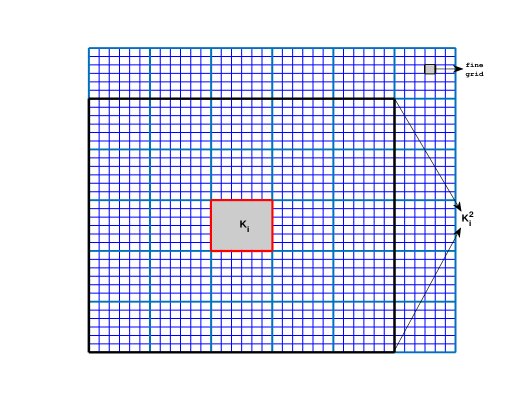
Let 𝒯hsubscript𝒯\mathcal{T}_{h} be a coarse gird partition of the space domain ΩΩ\Omega with Ncsubscript𝑁𝑐N_{c} nodes, N𝑁N elements, and hh the size of a generic coarse element. Figure 1 shows the fine gird, the coarse grid Kisubscript𝐾𝑖K_{i} and oversampling domain Kimsuperscriptsubscript𝐾𝑖𝑚K_{i}^{m} by enlarging coarse layers (m=2𝑚2m=2).

Refer to caption
Fig. 1: The fine gird, coarse grid Kisubscript𝐾𝑖K_{i}, oversampling domain Ki2superscriptsubscript𝐾𝑖2K_{i}^{2}

For each coarse block Ki𝒯hsubscript𝐾𝑖subscript𝒯K_{i}\in\mathcal{T}_{h}, we denote V(Ki):=H1(Ki)assign𝑉subscript𝐾𝑖superscript𝐻1subscript𝐾𝑖V(K_{i})\,:=\,H^{1}(K_{i}), and consider a set of auxiliary basis functions {ϕj(i)}j=1LiV(Ki)superscriptsubscriptsuperscriptsubscriptitalic-ϕ𝑗𝑖𝑗1subscript𝐿𝑖𝑉subscript𝐾𝑖\{{\phi}_{j}^{(i)}\}_{j=1}^{L_{i}}\in V(K_{i}) by solving the spectral problem

ai(ϕj(i),v)=λj(i)si(ϕj(i),v),vV(Ki),formulae-sequencesubscript𝑎𝑖superscriptsubscriptitalic-ϕ𝑗𝑖𝑣superscriptsubscript𝜆𝑗𝑖subscript𝑠𝑖superscriptsubscriptitalic-ϕ𝑗𝑖𝑣for-all𝑣𝑉subscript𝐾𝑖a_{i}({\phi}_{j}^{(i)},v)={\lambda}_{j}^{(i)}s_{i}({\phi}_{j}^{(i)},v),\quad\forall v\in V(K_{i}), (12)

where si(ϕj(i),v)=Kiκ~uvsubscript𝑠𝑖superscriptsubscriptitalic-ϕ𝑗𝑖𝑣subscriptsubscript𝐾𝑖~𝜅𝑢𝑣s_{i}(\phi_{j}^{(i)},v)=\int_{K_{i}}\tilde{\kappa}uv, and κ~=κi|Δχi|2~𝜅𝜅subscript𝑖superscriptΔsubscript𝜒𝑖2\tilde{\kappa}=\kappa\sum_{i}|\Delta{\chi}_{i}|^{2}, {χi}subscript𝜒𝑖\{{\chi}_{i}\} is a set of partition of unity functions for the coarse partition. We collect the first Lisubscript𝐿𝑖L_{i} eigenfunctions corresponding to the first Lisubscript𝐿𝑖L_{i} smallest eigenvalues for the local auxiliary multiscale space Vaux(i)=span{ϕj(i)|1jLi}superscriptsubscript𝑉𝑎𝑢𝑥𝑖spanconditional-setsuperscriptsubscriptitalic-ϕ𝑗𝑖1𝑗subscript𝐿𝑖V_{aux}^{(i)}=\text{span}\{\phi_{j}^{(i)}|1\leq j\leq L_{i}\} and define the global auxiliary space Vauxsubscript𝑉𝑎𝑢𝑥V_{aux} by the direct sum of these local spaces,

Vaux=i=1NVaux(i).subscript𝑉𝑎𝑢𝑥superscriptsubscriptdirect-sum𝑖1𝑁superscriptsubscript𝑉𝑎𝑢𝑥𝑖V_{aux}=\bigoplus_{i=1}^{N}V_{aux}^{(i)}.

Let the oversampling domain KimΩsuperscriptsubscript𝐾𝑖𝑚ΩK_{i}^{m}\subset\Omega be the extension of Kisubscript𝐾𝑖K_{i} with m𝑚m coarse grid layers (as in Figure 1). The CEM-MsFE basis functions φj,ms(i)H01(Kim)superscriptsubscript𝜑𝑗𝑚𝑠𝑖superscriptsubscript𝐻01superscriptsubscript𝐾𝑖𝑚\varphi_{j,ms}^{(i)}\in H_{0}^{1}(K_{i}^{m}) are constructed through solving the local problems

φj,ms(i)=argmin{a(φ,φ)|φH01(Kim),φ is ϕj(i)-orthogonal},superscriptsubscript𝜑𝑗𝑚𝑠𝑖conditional𝑎𝜑𝜑𝜑superscriptsubscript𝐻01superscriptsubscript𝐾𝑖𝑚𝜑 is superscriptsubscriptitalic-ϕ𝑗𝑖-orthogonal\varphi_{j,ms}^{(i)}=\arg\min\left\{\,a(\varphi,\varphi)\,|\,\varphi\in H_{0}^{1}(K_{i}^{m}),\,\varphi\text{ is }\phi_{j}^{(i)}\text{-orthogonal}\right\}, (13)

where φV𝜑𝑉\varphi\in V is ϕj(i)-orthogonalsuperscriptsubscriptitalic-ϕ𝑗𝑖-orthogonal\phi_{j}^{(i)}\text{-orthogonal} when

s(φ,ϕj(i))=1 and s(φ,ϕj(i))=0,if jj or ii,formulae-sequence𝑠𝜑superscriptsubscriptitalic-ϕ𝑗𝑖1 and formulae-sequence𝑠𝜑superscriptsubscriptitalic-ϕsuperscript𝑗superscript𝑖0if superscript𝑗𝑗 or superscript𝑖𝑖s(\varphi,\phi_{j}^{(i)})=1\quad\text{ and }\quad s(\varphi,\phi_{j^{\prime}}^{(i^{\prime})})=0,\quad\text{if }j^{\prime}\neq j\text{ or }i^{\prime}\neq i,

with s(u,v)=i=1Nsi(u,v).𝑠𝑢𝑣superscriptsubscript𝑖1𝑁subscript𝑠𝑖𝑢𝑣s(u,v)=\sum_{i=1}^{N}s_{i}(u,v). Thus, we define the multiscale finite element space for CEM-GMsFEM by

Vms= span {φj,ms(i)|1jLi, 1iN}.subscript𝑉𝑚𝑠 span conditional-setsuperscriptsubscript𝜑𝑗𝑚𝑠𝑖formulae-sequence1𝑗subscript𝐿𝑖1𝑖𝑁V_{ms}=\text{ span }\left\{\varphi_{j,ms}^{(i)}\,|1\leq j\leq L_{i},\,1\leq i\leq N\right\}.
Remark 3.1.

Lemma 5 in [10] implies that more layers m𝑚m of the oversampling domain Kimsuperscriptsubscript𝐾𝑖𝑚K_{i}^{m} can improve the approximation accuracy of the multiscale method. But the multiscale basis functions decay to zero on the oversampling domain as more layers are utilized [10, 29]. Thus, we may use a small number of layers for the oversampling domain to balance the approximation accuracy and computation efficiency.

3.2 A priori error analysis

In this subsection, we approximate the solution u(x,t)𝑢𝑥𝑡u(x,t) of the problem (10) by a function umsVmssubscript𝑢𝑚𝑠subscript𝑉𝑚𝑠u_{ms}\in V_{ms} for each t>0𝑡0t>0. First of all, we provide the error estimates of CEM-GMsFEM for the SPDE with multiplicative noise. To this end, we need some preliminary lemmas.

Lemma 4.

Let u𝑢u be the solution of the stochastic parabolic equation (1). Then

𝑬utL2(D×[0,T])2C(𝑬u0a2+f(u)2),𝑬subscriptsuperscriptnormsubscript𝑢𝑡2superscript𝐿2𝐷0𝑇𝐶𝑬superscriptsubscriptnormsubscript𝑢0𝑎2subscriptsuperscriptnorm𝑓𝑢2\bm{E}\|u_{t}\|^{2}_{L^{2}(D\times[0,T])}\leq C\bigg{(}\bm{E}\|u_{0}\|_{a}^{2}+\|f(u)\|^{2}_{\mathcal{H}}\bigg{)}, (14)

where ua2:=Dκ|u|2assignsuperscriptsubscriptnorm𝑢𝑎2subscript𝐷𝜅superscript𝑢2\|u\|_{a}^{2}:=\int_{D}\kappa|\nabla u|^{2} is the energy norm.

Proof.

By (10), we have

(ut,ut)+a(u,ut)=(f(u),ut)+(g(u)ξ(t),ut),subscript𝑢𝑡subscript𝑢𝑡𝑎𝑢subscript𝑢𝑡𝑓𝑢subscript𝑢𝑡𝑔𝑢𝜉𝑡subscript𝑢𝑡(u_{t},u_{t})+a(u,u_{t})=(f(u),u_{t})+(g(u)\xi(t),u_{t}),

which implies

utH2+12ddtua2=(f(u),ut)+(g(u)ξ(t),ut).subscriptsuperscriptnormsubscript𝑢𝑡2𝐻12𝑑𝑑𝑡superscriptsubscriptnorm𝑢𝑎2𝑓𝑢subscript𝑢𝑡𝑔𝑢𝜉𝑡subscript𝑢𝑡\|u_{t}\|^{2}_{H}+\frac{1}{2}\frac{d}{dt}\|u\|_{a}^{2}=(f(u),u_{t})+(g(u)\xi(t),u_{t}).

Integrating over the interval [0,t], 0tT0𝑡 0𝑡𝑇[0,t],\,0\leq t\leq T and taking the expectation of both sides, we get

𝑬0tut(x,s)H2𝑑s+12𝑬u(x,t)a2𝑬superscriptsubscript0𝑡subscriptsuperscriptnormsubscript𝑢𝑡𝑥𝑠2𝐻differential-d𝑠12𝑬superscriptsubscriptnorm𝑢𝑥𝑡𝑎2\displaystyle\bm{E}\int_{0}^{t}\|u_{t}(x,s)\|^{2}_{H}ds+\frac{1}{2}\bm{E}\|u(x,t)\|_{a}^{2}
=𝑬0t(f(u),ut)𝑑s+𝑬0t(g(u)ξ(s),ut)𝑑s+12𝑬u0a2absent𝑬superscriptsubscript0𝑡𝑓𝑢subscript𝑢𝑡differential-d𝑠𝑬superscriptsubscript0𝑡𝑔𝑢𝜉𝑠subscript𝑢𝑡differential-d𝑠12𝑬superscriptsubscriptnormsubscript𝑢0𝑎2\displaystyle=\bm{E}\int_{0}^{t}(f(u),u_{t})ds+\bm{E}\int_{0}^{t}(g(u)\xi(s),u_{t})ds+\frac{1}{2}\bm{E}\|u_{0}\|_{a}^{2}
=𝑬0t(f(u),ut)𝑑s+𝑬0t(g(u)dW(s),ut)+12𝑬u0a2absent𝑬superscriptsubscript0𝑡𝑓𝑢subscript𝑢𝑡differential-d𝑠𝑬superscriptsubscript0𝑡𝑔𝑢𝑑𝑊𝑠subscript𝑢𝑡12𝑬superscriptsubscriptnormsubscript𝑢0𝑎2\displaystyle=\bm{E}\int_{0}^{t}(f(u),u_{t})ds+\bm{E}\int_{0}^{t}(g(u)dW(s),u_{t})+\frac{1}{2}\bm{E}\|u_{0}\|_{a}^{2}
𝑬0t12(f(u)H2+utH2)𝑑s+12𝑬u0a2,absent𝑬superscriptsubscript0𝑡12subscriptsuperscriptnorm𝑓𝑢2𝐻subscriptsuperscriptnormsubscript𝑢𝑡2𝐻differential-d𝑠12𝑬superscriptsubscriptnormsubscript𝑢0𝑎2\displaystyle\leq\bm{E}\int_{0}^{t}\frac{1}{2}\left(\|f(u)\|^{2}_{H}+\|u_{t}\|^{2}_{H}\right)ds+\frac{1}{2}\bm{E}\|u_{0}\|_{a}^{2},

where 𝑬0t(g(u(s))dW(s),ut)=0𝑬superscriptsubscript0𝑡𝑔𝑢𝑠𝑑𝑊𝑠subscript𝑢𝑡0\bm{E}\int_{0}^{t}(g(u(s))dW(s),u_{t})=0 has been used in the third step by Prop.1. This completes the proof. ∎

Remark 3.2.

Since f(u)𝑓𝑢f(u) is of linear growth and a Nemytskii operator in H𝐻H and the weak solution of (2) uL([0,T],L2(D×Ω))𝑢superscript𝐿0𝑇superscript𝐿2𝐷Ωu\in L^{\infty}([0,T],L^{2}(D\times\Omega)), i.e., f(u)HCf(1+uH),uHformulae-sequencesubscriptnorm𝑓𝑢𝐻subscript𝐶𝑓1subscriptnorm𝑢𝐻for-all𝑢𝐻\left\|f(u)\right\|_{H}\leq C_{f}(1+\left\|u\right\|_{H}),\forall u\in H and supt[0,T]𝐄u(t)H2<+subscriptsupremum𝑡0𝑇𝐄superscriptsubscriptnorm𝑢𝑡𝐻2\sup_{t\in[0,T]}\bm{E}\left\|u(t)\right\|_{H}^{2}<+\infty, then further we have the following estimation by Lemma 4,

𝑬utL2(D×[0,T])2𝑬subscriptsuperscriptnormsubscript𝑢𝑡2superscript𝐿2𝐷0𝑇\displaystyle\bm{E}\|u_{t}\|^{2}_{L^{2}(D\times[0,T])} C(𝑬u0a2+f(u)2)absent𝐶𝑬superscriptsubscriptnormsubscript𝑢0𝑎2subscriptsuperscriptnorm𝑓𝑢2\displaystyle\leq C\bigg{(}\bm{E}\|u_{0}\|_{a}^{2}+\|f(u)\|^{2}_{\mathcal{H}}\bigg{)}
C(𝑬u0a2+2Cf(1+u2))absent𝐶𝑬superscriptsubscriptnormsubscript𝑢0𝑎22subscript𝐶𝑓1subscriptsuperscriptnorm𝑢2\displaystyle\leq C\bigg{(}\bm{E}\|u_{0}\|_{a}^{2}+2C_{f}(1+\|u\|^{2}_{\mathcal{H}})\bigg{)}
C(𝑬u0a2+2Cf(1+uL([0,T],L2(D×Ω))2))absent𝐶𝑬superscriptsubscriptnormsubscript𝑢0𝑎22subscript𝐶𝑓1subscriptsuperscriptnorm𝑢2superscript𝐿0𝑇superscript𝐿2𝐷Ω\displaystyle\leq C\bigg{(}\bm{E}\|u_{0}\|_{a}^{2}+2C_{f}\left(1+\|u\|^{2}_{L^{\infty}\left([0,T],L^{2}(D\times\Omega)\right)}\right)\bigg{)}
<+.absent\displaystyle<+\infty.

Let u^Vms^𝑢subscript𝑉𝑚𝑠\widehat{u}\in V_{ms} be the elliptic projection of the function uV𝑢𝑉u\in V, i.e., u^^𝑢\widehat{u} satisfies

a(u^,v)=a(u,v),vVms.formulae-sequence𝑎^𝑢𝑣𝑎𝑢𝑣for-all𝑣subscript𝑉𝑚𝑠a(\widehat{u},v)=a(u,v),\,\forall v\in V_{ms}.

From Lemma 4, we immediately have the following estimates of u^^𝑢\widehat{u} and umssubscript𝑢𝑚𝑠u_{ms}, respectively,

𝑬u^tL2(D×[0,T])2C(𝑬u^0a2+f(u)2),𝑬(ums)tL2(D×[0,T])2C(𝑬u0,msa2+f(u)2).formulae-sequence𝑬subscriptsuperscriptdelimited-∥∥subscript^𝑢𝑡2superscript𝐿2𝐷0𝑇𝐶𝑬superscriptsubscriptdelimited-∥∥subscript^𝑢0𝑎2subscriptsuperscriptdelimited-∥∥𝑓𝑢2𝑬subscriptsuperscriptdelimited-∥∥subscriptsubscript𝑢𝑚𝑠𝑡2superscript𝐿2𝐷0𝑇𝐶𝑬superscriptsubscriptdelimited-∥∥subscript𝑢0𝑚𝑠𝑎2subscriptsuperscriptdelimited-∥∥𝑓𝑢2\begin{split}\bm{E}\|\widehat{u}_{t}\|^{2}_{L^{2}(D\times[0,T])}&\>\leq C\bigg{(}\bm{E}\|\widehat{u}_{0}\|_{a}^{2}+\|f(u)\|^{2}_{\mathcal{H}}\bigg{)},\\ \bm{E}\|(u_{ms})_{t}\|^{2}_{L^{2}(D\times[0,T])}&\>\leq C\bigg{(}\bm{E}\|u_{0,ms}\|_{a}^{2}+\|f(u)\|^{2}_{\mathcal{H}}\bigg{)}.\end{split} (15)

By Lemma 4.34.34.3 in [29], we have the following estimate between the solution of stochastic parabolic equation and its corresponding elliptic projection.

Lemma 5.

Let u𝑢u be the solution of (1). For each t>0𝑡0t>0, any fixed realization ξ(t)𝜉𝑡\xi(t), the elliptic projection u^(t)Vms^𝑢𝑡subscript𝑉𝑚𝑠\widehat{u}(t)\in V_{ms} and satisfies

a(u(t)u^(t),v)=0,vVms.formulae-sequence𝑎𝑢𝑡^𝑢𝑡𝑣0for-all𝑣subscript𝑉𝑚𝑠a\big{(}u(t)-\widehat{u}(t),v\big{)}=0,\quad\forall v\in V_{ms}. (16)

Then, for any t>0𝑡0t>0,

(uu^)(t)aChΛ12κ12(f(u)+g(u)ξ(t)ut)(t)H,subscriptnorm𝑢^𝑢𝑡𝑎𝐶superscriptΛ12subscriptnormsuperscript𝜅12𝑓𝑢𝑔𝑢𝜉𝑡subscript𝑢𝑡𝑡𝐻\displaystyle\|(u-\widehat{u})(t)\|_{a}\leq Ch\Lambda^{-\frac{1}{2}}\|\kappa^{-\frac{1}{2}}(f(u)+g(u)\xi(t)-u_{t})(t)\|_{H},
(uu^)(t)HCh2Λ1κ012κ12(f(u)+g(u)ξ(t)ut)(t)H,subscriptnorm𝑢^𝑢𝑡𝐻𝐶superscript2superscriptΛ1superscriptsubscript𝜅012subscriptnormsuperscript𝜅12𝑓𝑢𝑔𝑢𝜉𝑡subscript𝑢𝑡𝑡𝐻\displaystyle\|(u-\widehat{u})(t)\|_{H}\leq Ch^{2}\Lambda^{-1}\kappa_{0}^{-\frac{1}{2}}\|\kappa^{-\frac{1}{2}}(f(u)+g(u)\xi(t)-u_{t})(t)\|_{H},

where C𝐶C is a constant independent of κ𝜅\kappa and the mesh size hh, and Λ=min1iNλLi+1(i)Λsubscript1𝑖𝑁superscriptsubscript𝜆subscript𝐿𝑖1𝑖\Lambda=\mathop{\min}\limits_{1\leq i\leq N}\lambda_{L_{i}+1}^{(i)} is the smallest eigenvalue that we discard when constructing the local auxiliary multiscale space.

Remark 3.3.

By Lemma 5 and Lemma 4, assuming g(u)ξ(t)𝑔𝑢𝜉𝑡g(u)\xi(t)\in\mathcal{H}, we further have the following estimations,

𝑬0t(uu^)(s)a2𝑑sCh2Λ1κ01(f(u)2+g(u)ξ(t)2+𝑬u0a2),𝑬superscriptsubscript0𝑡subscriptsuperscriptdelimited-∥∥𝑢^𝑢𝑠2𝑎differential-d𝑠𝐶superscript2superscriptΛ1superscriptsubscript𝜅01subscriptsuperscriptdelimited-∥∥𝑓𝑢2subscriptsuperscriptdelimited-∥∥𝑔𝑢𝜉𝑡2𝑬superscriptsubscriptdelimited-∥∥subscript𝑢0𝑎2\begin{split}\bm{E}\int_{0}^{t}\|(u-\widehat{u})(s)\|^{2}_{a}ds\leq Ch^{2}\Lambda^{-1}\kappa_{0}^{-1}\left(\|f(u)\|^{2}_{\mathcal{H}}+\|g(u)\xi(t)\|^{2}_{\mathcal{H}}+\bm{E}\|u_{0}\|_{a}^{2}\right),\end{split} (17)
𝑬0t(uu^)(s)H2𝑑sCh4Λ2κ02(f(u)2+g(u)ξ(t)2+𝑬u0a2).𝑬superscriptsubscript0𝑡subscriptsuperscriptnorm𝑢^𝑢𝑠2𝐻differential-d𝑠𝐶superscript4superscriptΛ2superscriptsubscript𝜅02subscriptsuperscriptnorm𝑓𝑢2subscriptsuperscriptnorm𝑔𝑢𝜉𝑡2𝑬superscriptsubscriptnormsubscript𝑢0𝑎2\bm{E}\int_{0}^{t}\|(u-\widehat{u})(s)\|^{2}_{H}ds\leq Ch^{4}\Lambda^{-2}\kappa_{0}^{-2}\left(\|f(u)\|^{2}_{\mathcal{H}}+\|g(u)\xi(t)\|^{2}_{\mathcal{H}}+\bm{E}\|u_{0}\|_{a}^{2}\right). (18)

In the following theorem, we prove a strong convergence of the semidiscrete solution of (11).

Theorem 6.

Let u𝑢u and umssubscript𝑢𝑚𝑠u_{ms} be the solution of (10) and (11), respectively. Then for any fixed t[0,T]𝑡0𝑇t\in[0,T],

𝑬(uums)(t)H2+𝑬0tuumsa2𝑑sCh2Λ1κ01(f(u)2+g(u)ξ(x,t)2+𝑬u0a2+𝑬u0,msa2)+𝑬(uums)(0)H2,𝑬superscriptsubscriptdelimited-∥∥𝑢subscript𝑢𝑚𝑠𝑡𝐻2𝑬superscriptsubscript0𝑡superscriptsubscriptdelimited-∥∥𝑢subscript𝑢𝑚𝑠𝑎2differential-d𝑠𝐶superscript2superscriptΛ1superscriptsubscript𝜅01subscriptsuperscriptdelimited-∥∥𝑓𝑢2subscriptsuperscriptdelimited-∥∥𝑔𝑢𝜉𝑥𝑡2𝑬superscriptsubscriptdelimited-∥∥subscript𝑢0𝑎2𝑬superscriptsubscriptdelimited-∥∥subscript𝑢0𝑚𝑠𝑎2𝑬superscriptsubscriptdelimited-∥∥𝑢subscript𝑢𝑚𝑠0𝐻2\begin{split}&\>\bm{E}\|(u-u_{ms})(t)\|_{H}^{2}+\bm{E}\int_{0}^{t}\|u-u_{ms}\|_{a}^{2}ds\\ &\>\leq Ch^{2}\Lambda^{-1}\kappa_{0}^{-1}\left(\|f(u)\|^{2}_{\mathcal{H}}+\|g(u)\xi(x,t)\|^{2}_{\mathcal{H}}+\bm{E}\|u_{0}\|_{a}^{2}+\bm{E}\|u_{0,ms}\|_{a}^{2}\right)\\ \quad&\>+\bm{E}\|(u-u_{ms})(0)\|_{H}^{2},\end{split} (19)

where C𝐶C is a constant independent of κ𝜅\kappa and the mesh size hh.

Proof.

By (10) and (11), we have

(ut,v)+a(u,v)subscript𝑢𝑡𝑣𝑎𝑢𝑣\displaystyle(u_{t},v)+a(u,v) =(f(u),v)+(g(u)ξ(t),v),absent𝑓𝑢𝑣𝑔𝑢𝜉𝑡𝑣\displaystyle=\big{(}f(u),v\big{)}+\big{(}g(u)\xi(t),v\big{)}, (20)
((ums)t,v)+a(ums,v)subscriptsubscript𝑢𝑚𝑠𝑡𝑣𝑎subscript𝑢𝑚𝑠𝑣\displaystyle\big{(}(u_{ms})_{t},v\big{)}+a(u_{ms},v) =(f(ums),v)+(g(ums)ξ(t),v)absent𝑓subscript𝑢𝑚𝑠𝑣𝑔subscript𝑢𝑚𝑠𝜉𝑡𝑣\displaystyle=\big{(}f(u_{ms}),v\big{)}+\big{(}g(u_{ms})\xi(t),v\big{)} (21)

for all vVms𝑣subscript𝑉𝑚𝑠v\in V_{ms}. Thus, by subtracting (21) from (20), we get, for vVmsfor-all𝑣subscript𝑉𝑚𝑠\forall v\,\in V_{ms}

((uums)t,v)+a(uums,v)=(f(u)f(ums),v)+(g(u)ξg(ums)ξ,v).subscript𝑢subscript𝑢𝑚𝑠𝑡𝑣𝑎𝑢subscript𝑢𝑚𝑠𝑣𝑓𝑢𝑓subscript𝑢𝑚𝑠𝑣𝑔𝑢𝜉𝑔subscript𝑢𝑚𝑠𝜉𝑣\big{(}(u-u_{ms})_{t},v\big{)}+a(u-u_{ms},v)=\big{(}f(u)-f(u_{ms}),v\big{)}+\big{(}g(u)\xi-g(u_{ms})\xi,v\big{)}. (22)

The elliptic projection of u𝑢u, u^Vms^𝑢subscript𝑉𝑚𝑠\widehat{u}\in V_{ms}, satisfies (17) and (18). In particular, by taking v=u^umsVms𝑣^𝑢subscript𝑢𝑚𝑠subscript𝑉𝑚𝑠v=\widehat{u}-u_{ms}\in V_{ms} in (22), we have the following error equation,

((uums)t,u^ums)+a(uums,u^ums)=(f(u)f(ums),u^ums)+((g(u)g(ums))ξ,u^ums).subscript𝑢subscript𝑢𝑚𝑠𝑡^𝑢subscript𝑢𝑚𝑠𝑎𝑢subscript𝑢𝑚𝑠^𝑢subscript𝑢𝑚𝑠𝑓𝑢𝑓subscript𝑢𝑚𝑠^𝑢subscript𝑢𝑚𝑠𝑔𝑢𝑔subscript𝑢𝑚𝑠𝜉^𝑢subscript𝑢𝑚𝑠\begin{split}&\big{(}(u-u_{ms})_{t},\widehat{u}-u_{ms}\big{)}+\>a(u-u_{ms},\widehat{u}-u_{ms})\\ =&\>\big{(}f(u)-f(u_{ms}),\widehat{u}-u_{ms}\big{)}+\Big{(}\big{(}g(u)-g(u_{ms})\big{)}\xi,\widehat{u}-u_{ms}\Big{)}.\end{split} (23)

Due to the bilinearity of a(,)𝑎a(\cdot,\cdot), we can rewrite (23) as

((uums)t,uums)+a(uums,uums)+(f(ums)f(u),uums)+((g(ums)g(u))ξ,uums)=((uums)t,uu^)+a(uums,uu^)+(f(ums)f(u),uu^)+((g(ums)g(u))ξ,uu^).subscript𝑢subscript𝑢𝑚𝑠𝑡𝑢subscript𝑢𝑚𝑠𝑎𝑢subscript𝑢𝑚𝑠𝑢subscript𝑢𝑚𝑠𝑓subscript𝑢𝑚𝑠𝑓𝑢𝑢subscript𝑢𝑚𝑠𝑔subscript𝑢𝑚𝑠𝑔𝑢𝜉𝑢subscript𝑢𝑚𝑠subscript𝑢subscript𝑢𝑚𝑠𝑡𝑢^𝑢𝑎𝑢subscript𝑢𝑚𝑠𝑢^𝑢𝑓subscript𝑢𝑚𝑠𝑓𝑢𝑢^𝑢𝑔subscript𝑢𝑚𝑠𝑔𝑢𝜉𝑢^𝑢\begin{split}&\>\big{(}(u-u_{ms})_{t},u-u_{ms}\big{)}+a(u-u_{ms},u-u_{ms})\\ &\>+\big{(}f(u_{ms})-f(u),u-u_{ms}\big{)}+\Big{(}\big{(}g(u_{ms})-g(u)\big{)}\xi,u-u_{ms}\Big{)}\\ =&\>\big{(}(u-u_{ms})_{t},u-\widehat{u}\big{)}+a(u-u_{ms},u-\widehat{u})\\ &\>+\big{(}f(u_{ms})-f(u),u-\widehat{u}\big{)}+\Big{(}\big{(}g(u_{ms})-g(u)\big{)}\xi,u-\widehat{u}\Big{)}.\end{split}

The Lipschitz assumptions of f𝑓f, Cauchy-Schwarz inequality and Young’s inequality give

12ddtuums2+uumsa2Lfuums2+((g(ums)g(u))ξ,uums)((uums)t,uu^)+a(uums,uu^)+12Lfuums2+12uu^2+((g(ums)g(u))ξ,uu^).12𝑑𝑑𝑡superscriptdelimited-∥∥𝑢subscript𝑢𝑚𝑠2superscriptsubscriptdelimited-∥∥𝑢subscript𝑢𝑚𝑠𝑎2subscript𝐿𝑓superscriptdelimited-∥∥𝑢subscript𝑢𝑚𝑠2𝑔subscript𝑢𝑚𝑠𝑔𝑢𝜉𝑢subscript𝑢𝑚𝑠subscript𝑢subscript𝑢𝑚𝑠𝑡𝑢^𝑢𝑎𝑢subscript𝑢𝑚𝑠𝑢^𝑢12subscript𝐿𝑓superscriptdelimited-∥∥𝑢subscript𝑢𝑚𝑠212superscriptdelimited-∥∥𝑢^𝑢2𝑔subscript𝑢𝑚𝑠𝑔𝑢𝜉𝑢^𝑢\begin{split}&\>\frac{1}{2}\frac{d}{dt}\|u-u_{ms}\|^{2}+\|u-u_{ms}\|_{a}^{2}-L_{f}\|u-u_{ms}\|^{2}+\Big{(}\big{(}g(u_{ms})-g(u)\big{)}\xi,u-u_{ms}\Big{)}\\ \leq&\>\big{(}(u-u_{ms})_{t},u-\widehat{u}\big{)}+a(u-u_{ms},u-\widehat{u})+\frac{1}{2}L_{f}\|u-u_{ms}\|^{2}+\frac{1}{2}\|u-\widehat{u}\|^{2}\\ &\>+\Big{(}\big{(}g(u_{ms})-g(u)\big{)}\xi,u-\widehat{u}\Big{)}.\end{split}

After taking integration over [0,t]0𝑡[0,t] for t, 0tTfor-all𝑡 0𝑡𝑇\forall t,\,0\leq t\leq T, and taking expectation with respect to random process, and using the Cauchy-Schwarz and Young’s inequalities to the right-hand side, it follows that

𝑬(uums)(t)H2+𝑬0tuumsa2𝑑s2𝑬0t(utH+(ums)tH)uu^H𝑑s+𝑬0tuu^a2𝑑s+𝑬0tuu^H2𝑑s+3Lf𝑬0tuumsH2𝑑s+𝑬(uums)(0)H2,𝑬superscriptsubscriptdelimited-∥∥𝑢subscript𝑢𝑚𝑠𝑡𝐻2𝑬superscriptsubscript0𝑡superscriptsubscriptdelimited-∥∥𝑢subscript𝑢𝑚𝑠𝑎2differential-d𝑠2𝑬superscriptsubscript0𝑡subscriptdelimited-∥∥subscript𝑢𝑡𝐻subscriptdelimited-∥∥subscriptsubscript𝑢𝑚𝑠𝑡𝐻subscriptdelimited-∥∥𝑢^𝑢𝐻differential-d𝑠𝑬superscriptsubscript0𝑡superscriptsubscriptdelimited-∥∥𝑢^𝑢𝑎2differential-d𝑠𝑬superscriptsubscript0𝑡superscriptsubscriptdelimited-∥∥𝑢^𝑢𝐻2differential-d𝑠3subscript𝐿𝑓𝑬superscriptsubscript0𝑡superscriptsubscriptdelimited-∥∥𝑢subscript𝑢𝑚𝑠𝐻2differential-d𝑠𝑬superscriptsubscriptdelimited-∥∥𝑢subscript𝑢𝑚𝑠0𝐻2\begin{split}&\bm{E}\|(u-u_{ms})(t)\|_{H}^{2}+\bm{E}\int_{0}^{t}\|u-u_{ms}\|_{a}^{2}ds\\ &\leq 2\bm{E}\int_{0}^{t}(\|u_{t}\|_{H}+\|(u_{ms})_{t}\|_{H})\|u-\widehat{u}\|_{H}ds+\bm{E}\int_{0}^{t}\|u-\widehat{u}\|_{a}^{2}ds+\bm{E}\int_{0}^{t}\|u-\widehat{u}\|_{H}^{2}ds\\ &+3L_{f}\bm{E}\int_{0}^{t}\|u-u_{ms}\|_{H}^{2}ds+\bm{E}\|(u-u_{ms})(0)\|_{H}^{2},\end{split} (24)

where we used the following result by Prop.1,

𝑬0t((g(ums)g(u))ξ(s),uums)𝑑s=𝑬0t((g(ums)g(u))dW(s),uums),𝑬superscriptsubscript0𝑡𝑔subscript𝑢𝑚𝑠𝑔𝑢𝜉𝑠𝑢subscript𝑢𝑚𝑠differential-d𝑠𝑬superscriptsubscript0𝑡𝑔subscript𝑢𝑚𝑠𝑔𝑢𝑑𝑊𝑠𝑢subscript𝑢𝑚𝑠\displaystyle\bm{E}\int_{0}^{t}\Big{(}\big{(}g(u_{ms})-g(u)\big{)}\xi(s),u-u_{ms}\Big{)}ds=\bm{E}\int_{0}^{t}\Big{(}\big{(}g(u_{ms})-g(u)\big{)}dW(s),u-u_{ms}\Big{)},
𝑬0t((g(ums)g(u))ξ(s),uu^)𝑑s=𝑬0t((g(ums)g(u))dW(s),uu^).𝑬superscriptsubscript0𝑡𝑔subscript𝑢𝑚𝑠𝑔𝑢𝜉𝑠𝑢^𝑢differential-d𝑠𝑬superscriptsubscript0𝑡𝑔subscript𝑢𝑚𝑠𝑔𝑢𝑑𝑊𝑠𝑢^𝑢\displaystyle\bm{E}\int_{0}^{t}\Big{(}\big{(}g(u_{ms})-g(u)\big{)}\xi(s),u-\widehat{u}\Big{)}ds=\bm{E}\int_{0}^{t}\Big{(}\big{(}g(u_{ms})-g(u)\big{)}dW(s),u-\widehat{u}\Big{)}.

For the first term on the right-hand side of (24), Ho¨¨𝑜\ddot{o}lder inequality implies

𝑬0t(utH+(ums)tH)uu^H𝑑s𝑬{(0t(utH+(ums)tH)2𝑑s)12(0tuu^H2𝑑s)12}.𝑬superscriptsubscript0𝑡subscriptdelimited-∥∥subscript𝑢𝑡𝐻subscriptdelimited-∥∥subscriptsubscript𝑢𝑚𝑠𝑡𝐻subscriptdelimited-∥∥𝑢^𝑢𝐻differential-d𝑠𝑬superscriptsuperscriptsubscript0𝑡superscriptsubscriptdelimited-∥∥subscript𝑢𝑡𝐻subscriptdelimited-∥∥subscriptsubscript𝑢𝑚𝑠𝑡𝐻2differential-d𝑠12superscriptsuperscriptsubscript0𝑡superscriptsubscriptdelimited-∥∥𝑢^𝑢𝐻2differential-d𝑠12\begin{split}&\bm{E}\int_{0}^{t}\big{(}\|u_{t}\|_{H}\>+\|(u_{ms})_{t}\|_{H}\big{)}\|u-\widehat{u}\|_{H}ds\\ &\>\leq\bm{E}\left\{\left(\int_{0}^{t}\big{(}\|u_{t}\|_{H}+\|(u_{ms})_{t}\|_{H}\big{)}^{2}ds\right)^{\frac{1}{2}}\left(\int_{0}^{t}\|u-\widehat{u}\|_{H}^{2}ds\right)^{\frac{1}{2}}\right\}.\end{split} (25)

For presentation convenience, we define

I:= 2𝑬{(0t(utH+(ums)tH)2𝑑s)12(0tuu^H2𝑑s)12}+𝑬0tuu^a2𝑑s+𝑬0tuu^H2𝑑s+𝑬(uums)(0)H2.assign𝐼2𝑬superscriptsuperscriptsubscript0𝑡superscriptsubscriptdelimited-∥∥subscript𝑢𝑡𝐻subscriptdelimited-∥∥subscriptsubscript𝑢𝑚𝑠𝑡𝐻2differential-d𝑠12superscriptsuperscriptsubscript0𝑡superscriptsubscriptdelimited-∥∥𝑢^𝑢𝐻2differential-d𝑠12𝑬superscriptsubscript0𝑡superscriptsubscriptdelimited-∥∥𝑢^𝑢𝑎2differential-d𝑠𝑬superscriptsubscript0𝑡superscriptsubscriptdelimited-∥∥𝑢^𝑢𝐻2differential-d𝑠𝑬superscriptsubscriptdelimited-∥∥𝑢subscript𝑢𝑚𝑠0𝐻2\begin{split}I:=&\>2\bm{E}\left\{\left(\int_{0}^{t}\big{(}\|u_{t}\|_{H}+\|(u_{ms})_{t}\|_{H}\big{)}^{2}ds\right)^{\frac{1}{2}}\left(\int_{0}^{t}\|u-\widehat{u}\|_{H}^{2}ds\right)^{\frac{1}{2}}\right\}\\ &\>+\bm{E}\int_{0}^{t}\|u-\widehat{u}\|_{a}^{2}ds+\bm{E}\int_{0}^{t}\|u-\widehat{u}\|_{H}^{2}ds+\bm{E}\|(u-u_{ms})(0)\|_{H}^{2}.\end{split} (26)

Hence, from (24), (25) and (26), we get

𝑬(uums)(t)H2+𝑬0tuumsa2𝑑sI+3Lf𝑬0tuumsH2𝑑sI+3Lf𝑬0t(uumsH2+0tuumsa2𝑑τ)𝑑s.𝑬superscriptsubscriptdelimited-∥∥𝑢subscript𝑢𝑚𝑠𝑡𝐻2𝑬superscriptsubscript0𝑡superscriptsubscriptdelimited-∥∥𝑢subscript𝑢𝑚𝑠𝑎2differential-d𝑠𝐼3subscript𝐿𝑓𝑬superscriptsubscript0𝑡superscriptsubscriptdelimited-∥∥𝑢subscript𝑢𝑚𝑠𝐻2differential-d𝑠𝐼3subscript𝐿𝑓𝑬superscriptsubscript0𝑡superscriptsubscriptdelimited-∥∥𝑢subscript𝑢𝑚𝑠𝐻2superscriptsubscript0𝑡superscriptsubscriptdelimited-∥∥𝑢subscript𝑢𝑚𝑠𝑎2differential-d𝜏differential-d𝑠\begin{split}\bm{E}\|(u-u_{ms})(t)\|_{H}^{2}+&\>\bm{E}\int_{0}^{t}\|u-u_{ms}\|_{a}^{2}ds\leq I+3L_{f}\bm{E}\int_{0}^{t}\|u-u_{ms}\|_{H}^{2}ds\\ &\>\leq I+3L_{f}\bm{E}\int_{0}^{t}\left(\|u-u_{ms}\|_{H}^{2}+\int_{0}^{t}\|u-u_{ms}\|_{a}^{2}d\tau\right)ds.\end{split}

The Gronwall inequality concludes that

𝑬(uums)(t)H2+𝑬0tuumsa2𝑑s𝒞I.𝑬superscriptsubscriptnorm𝑢subscript𝑢𝑚𝑠𝑡𝐻2𝑬superscriptsubscript0𝑡superscriptsubscriptnorm𝑢subscript𝑢𝑚𝑠𝑎2differential-d𝑠𝒞𝐼\bm{E}\|(u-u_{ms})(t)\|_{H}^{2}+\bm{E}\int_{0}^{t}\|u-u_{ms}\|_{a}^{2}ds\leq\mathcal{C}I. (27)

Finally, combining Lemma 4, Corollary 15, Lemma 5, Remark 3.3 and (27), we complete the proof. ∎

In particular, for stochastic parabolic PDEs with additive noise, which is the degeneration of (1), i.e.,

{du(κ(x)u)dt=f(u)dt+g(x,t)dW(t)inD×(0,T],u(x,t)=0onD×(0,T],u(x,0)=u0(x)inD.\left\{\begin{aligned} du-\nabla\cdot\big{(}\kappa(x)\nabla u\big{)}dt&=f(u)dt+g(x,t)dW(t)\quad in\quad D\times(0,T],\\ u(x,t)&=0\quad on\quad\partial D\times(0,T],\\ u(x,0)&=u_{0}(x)\quad in\quad D.\end{aligned}\right. (28)

We similarly have the variational form of (28)

{(ut,v)+a(u,v)=(f(u),v)+(g(x,t)ξ(t),v)vH01,t>0,(u(,0),v)=(u0,v)vH01,\left\{\begin{aligned} (u_{t},v)+a(u,v)&=\big{(}f(u),v\big{)}+\big{(}g(x,t)\xi(t),v\big{)}\quad\forall v\in H_{0}^{1},\,t>0,\\ \big{(}u(\cdot,0),v\big{)}&=(u_{0},v)\quad\forall v\in H_{0}^{1},\end{aligned}\right. (29)

Then CEM-GMsFEM solution u(,t)Vms𝑢𝑡subscript𝑉𝑚𝑠u(\cdot,t)\in V_{ms} of (29) solves

{((ums)t,v)+a(ums,v)=(f(ums),v)+(g(x,t)ξ(t),v)vVms,t>0,(ums(,0),v)=(u0,ms,v)vVms\left\{\begin{aligned} \big{(}(u_{ms})_{t},v\big{)}+a(u_{ms},v)&=\big{(}f(u_{ms}),v\big{)}+\big{(}g(x,t)\xi(t),v\big{)}\quad\forall v\in V_{ms},\,t>0,\\ \big{(}u_{ms}(\cdot,0),v\big{)}&=(u_{0,ms},v)\quad\forall v\in V_{ms}\end{aligned}\right. (30)

We have the following error estimate of CEM-GMsFEM for the SPDE with additive noise, which generalizes the result in [42].

Theorem 7.

Let u𝑢u and umssubscript𝑢𝑚𝑠u_{ms} be the solution of (29) and (30), respectively. Then for any fixed t[0,T]𝑡0𝑇t\in[0,T],

𝑬(uums)(t)H2+𝑬0tuumsa2𝑑sCh2Λ1κ01(f(u)2+𝑬u0a2+𝑬u0,msa2)+𝑬(uums)(0)H2,𝑬superscriptsubscriptdelimited-∥∥𝑢subscript𝑢𝑚𝑠𝑡𝐻2𝑬superscriptsubscript0𝑡superscriptsubscriptdelimited-∥∥𝑢subscript𝑢𝑚𝑠𝑎2differential-d𝑠𝐶superscript2superscriptΛ1superscriptsubscript𝜅01subscriptsuperscriptdelimited-∥∥𝑓𝑢2𝑬superscriptsubscriptdelimited-∥∥subscript𝑢0𝑎2𝑬superscriptsubscriptdelimited-∥∥subscript𝑢0𝑚𝑠𝑎2𝑬superscriptsubscriptdelimited-∥∥𝑢subscript𝑢𝑚𝑠0𝐻2\begin{split}&\>\bm{E}\|(u-u_{ms})(t)\|_{H}^{2}+\bm{E}\int_{0}^{t}\|u-u_{ms}\|_{a}^{2}ds\\ &\>\leq Ch^{2}\Lambda^{-1}\kappa_{0}^{-1}\left(\|f(u)\|^{2}_{\mathcal{H}}+\bm{E}\|u_{0}\|_{a}^{2}+\bm{E}\|u_{0,ms}\|_{a}^{2}\right)+\bm{E}\|(u-u_{ms})(0)\|_{H}^{2},\end{split} (31)

where C𝐶C is a constant independent of κ𝜅\kappa and the mesh size hh.

Proof.

From (29) and (30), for vVmsfor-all𝑣subscript𝑉𝑚𝑠\forall v\,\in V_{ms}, we have

((uums)t,v)+a(uums,v)=(f(u)f(ums),v).subscript𝑢subscript𝑢𝑚𝑠𝑡𝑣𝑎𝑢subscript𝑢𝑚𝑠𝑣𝑓𝑢𝑓subscript𝑢𝑚𝑠𝑣\big{(}(u-u_{ms})_{t},v\big{)}+a(u-u_{ms},v)=\big{(}f(u)-f(u_{ms}),v\big{)}. (32)

The noise term disappears because diffusion g(x,t)𝑔𝑥𝑡g(x,t) is independent of the state u𝑢u. By following the proof of Theorem 6, the proof is done. ∎

4 Model reduction for nonlinear terms

Let {φi(x)}i=1Nrsuperscriptsubscriptsubscript𝜑𝑖𝑥𝑖1subscript𝑁𝑟\{\varphi_{i}(x)\}_{i=1}^{N_{r}} be the set of multiscale basis functions in CEM-GMsFEM. Then we have an approximation,

uums=i=1Nrumsi(t)φi(x).𝑢subscript𝑢𝑚𝑠superscriptsubscript𝑖1subscript𝑁𝑟subscriptsuperscript𝑢𝑖𝑚𝑠𝑡subscript𝜑𝑖𝑥u\approx u_{ms}=\sum_{i=1}^{N_{r}}u^{i}_{ms}(t)\varphi_{i}(x).

After we apply CEM-GMsFEM to SPDE(1), CEM-GMsFEM yields a discrete dynamical system of nonlinear ODE:

{𝐌d𝐮𝐦𝐬dt+A𝐮𝐦𝐬(t)=𝐅(𝐮𝐦𝐬(t))𝐮𝐦𝐬𝟎=𝐮𝐦𝐬(0),\left\{\begin{aligned} \mathbf{M}\frac{d\mathbf{u_{ms}}}{dt}+A\mathbf{u_{ms}}(t)&=\mathbf{F}(\mathbf{u_{ms}}(t))\\ \mathbf{u_{ms}^{0}}&=\mathbf{u_{ms}}(0),\end{aligned}\right. (33)

where 𝐮𝐦𝐬=[ums1,ums2,,umsNr]TNrsubscript𝐮𝐦𝐬superscriptsubscriptsuperscript𝑢1𝑚𝑠subscriptsuperscript𝑢2𝑚𝑠subscriptsuperscript𝑢subscript𝑁𝑟𝑚𝑠𝑇superscriptsubscript𝑁𝑟\mathbf{u_{ms}}=[u^{1}_{ms},u^{2}_{ms},\cdots,u^{N_{r}}_{ms}]^{T}\in\mathbb{R}^{N_{r}} and

𝐌ijsubscript𝐌𝑖𝑗\displaystyle\mathbf{M}_{ij} =Dφi(x)φj(x),absentsubscript𝐷subscript𝜑𝑖𝑥subscript𝜑𝑗𝑥\displaystyle=\int_{D}\varphi_{i}(x)\varphi_{j}(x),
Aijsubscript𝐴𝑖𝑗\displaystyle A_{ij} =Dκ(x)φi(x)φj(x),absentsubscript𝐷𝜅𝑥subscript𝜑𝑖𝑥subscript𝜑𝑗𝑥\displaystyle=\int_{D}\kappa(x)\nabla\varphi_{i}(x)\nabla\varphi_{j}(x),
𝐅(𝐮𝐦𝐬(t))i𝐅subscriptsubscript𝐮𝐦𝐬𝑡𝑖\displaystyle{\mathbf{F}(\mathbf{u_{ms}}(t))}_{i} D(f(l=1Nrumslφl(x))+g(l=1Nrumslφl(x))ξ(t))φi(x).absentsubscript𝐷𝑓superscriptsubscript𝑙1subscript𝑁𝑟subscriptsuperscript𝑢𝑙𝑚𝑠subscript𝜑𝑙𝑥𝑔superscriptsubscript𝑙1subscript𝑁𝑟subscriptsuperscript𝑢𝑙𝑚𝑠subscript𝜑𝑙𝑥𝜉𝑡subscript𝜑𝑖𝑥\displaystyle\approx\int_{D}\bigg{(}f\big{(}\sum_{l=1}^{N_{r}}u^{l}_{ms}\varphi_{l}(x)\big{)}+g\big{(}\sum_{l=1}^{N_{r}}u^{l}_{ms}\varphi_{l}(x)\big{)}\xi(t)\bigg{)}\varphi_{i}(x).

Notice that 𝐌,ANr×Nr𝐌𝐴superscriptsubscript𝑁𝑟subscript𝑁𝑟\mathbf{M},\,A\in\mathbb{R}^{N_{r}\times N_{r}}, and 𝐅:NrNr:𝐅superscriptsubscript𝑁𝑟superscriptsubscript𝑁𝑟\mathbf{F}:\mathbb{R}^{N_{r}}\rightarrow\mathbb{R}^{N_{r}} is a nonlinear function. Although Nrsubscript𝑁𝑟N_{r}, number of multiscale basis functions, is usually much smaller than number of fine-grid FEM basis functions, computation of the above system (33) is still challenging because the high-dimensionality is still in the nonlinear term and we need to compute many trajectories for statistical estimation of the solution. Thus it is desirable to significantly reduce the nonlinear dynamic system.

In this section, we first briefly review two important model reduction methods: POD and DEIM. Finally we introduce a stochastic online DEIM, which can substantially improve the computation efficiency of the nonlinear stochastic system (33). For simplicity of presentation, we rewrite the system (33) by

d𝐲dt=A𝐲(t)+𝐟(𝐲(t)).𝑑𝐲𝑑𝑡𝐴𝐲𝑡𝐟𝐲𝑡\frac{d\mathbf{y}}{dt}=A\mathbf{y}(t)+\mathbf{f}(\mathbf{y}(t)). (34)

Here we have abused the notation for linear coefficient matrix A𝐴A and nonlinear function 𝐟𝐟\mathbf{f} corresponding to 𝐌1Asuperscript𝐌1𝐴\mathbf{M}^{-1}A and 𝐌1𝐅superscript𝐌1𝐅\mathbf{M}^{-1}\mathbf{F} respectively in (33), and 𝐲𝐲\mathbf{y} represent the unknown solution that we are interested in.

4.1 Proper orthogonal decomposition

In the POD approach, we simulate the system by a reduced basis. Let {𝐲(ti)}i=1Msuperscriptsubscript𝐲subscript𝑡𝑖𝑖1𝑀\{\mathbf{y}(t_{i})\}_{i=1}^{M} be the solution vectors at M𝑀M time levels, and

Y=[𝐲(t1),𝐲(t2),,𝐲(tM)]n×M𝑌𝐲subscript𝑡1𝐲subscript𝑡2𝐲subscript𝑡𝑀superscript𝑛𝑀Y=[\mathbf{y}(t_{1}),\mathbf{y}(t_{2}),\cdots,\mathbf{y}(t_{M})]\in\mathbb{R}^{n\times M}

be the snapshot matrix. POD constructs an orthogonal basis Vn×r𝑉superscript𝑛𝑟V\in\mathbb{R}^{n\times r}, in which the basis vectors are the first rrank(Y)𝑟rank𝑌r\leq\text{rank}(Y) left singular vectors of Y𝑌Y corresponding to the first r𝑟r largest singular values. The basis is also a solution of the following minimization problem

minVn×r,VTV=Ir(InVVT)YF2.subscriptformulae-sequence𝑉superscript𝑛𝑟superscript𝑉𝑇𝑉subscript𝐼𝑟superscriptsubscriptnormsubscript𝐼𝑛𝑉superscript𝑉𝑇𝑌𝐹2\min_{V\in\mathbb{R}^{n\times r},V^{T}V=I_{r}}\|(I_{n}-VV^{T})Y\|_{F}^{2}.

Thus POD-Galerkin method gives a reduced system of (34)

d𝐲^dt=VTAV𝐲^(t)+VT𝐟(V𝐲^(t)),𝑑^𝐲𝑑𝑡superscript𝑉𝑇𝐴𝑉^𝐲𝑡superscript𝑉𝑇𝐟𝑉^𝐲𝑡\frac{d\hat{\mathbf{y}}}{dt}=V^{T}AV\hat{\mathbf{y}}(t)+V^{T}\mathbf{f}(V\hat{\mathbf{y}}(t)), (35)

and the solution 𝐲(t)𝐲𝑡\mathbf{y}(t) of (34) is approximated by 𝐲(t)V𝐲^(t)𝐲𝑡𝑉^𝐲𝑡\mathbf{y}(t)\approx V\hat{\mathbf{y}}(t). However, solving the reduced system (35) instead of (34), we still need evaluations of the nonlinear term 𝐟𝐟\mathbf{f} at all n𝑛n components, the simulation of (35) is as expensive as solving the original system. DEIM can be used to overcome this difficulty.

4.2 Discrete empirical interpolation method

DEIM provides an approximation of the nonlinear function 𝐟𝐟\mathbf{f} by a projection (interpolation), which maps a high nlimit-from𝑛n-dim space to a low mlimit-from𝑚m-dim space (mnmuch-less-than𝑚𝑛m\ll n) spanned by the basis 𝐔=[𝐮1,𝐮2,,𝐮m]n×m𝐔subscript𝐮1subscript𝐮2subscript𝐮𝑚superscript𝑛𝑚\mathbf{U}=[\mathbf{u}_{1},\mathbf{u}_{2},\cdots,\mathbf{u}_{m}]\in\mathbb{R}^{n\times m}. DEIM gives

𝐟𝐔𝐜,𝐟𝐔𝐜\mathbf{f}\approx\mathbf{U}\mathbf{c}, (36)

where 𝐜𝐜\mathbf{c} is an unknown vector. The projection basis 𝐔𝐔\mathbf{U} is obtained by applying POD to an appropriate set of the nonliear snapshots

{𝐟(𝐲(t1)),,𝐟(𝐲(tM))}n.𝐟𝐲subscript𝑡1𝐟𝐲subscript𝑡𝑀superscript𝑛\{\mathbf{f}(\mathbf{y}(t_{1})),\cdots,\mathbf{f}(\mathbf{y}(t_{M}))\}\subset\mathbb{R}^{n}.

The system (36) is overdetermined. In order to solve it, we multiplies the equation by the transpose of the matrix Pn×m𝑃superscript𝑛𝑚P\in\mathbb{R}^{n\times m},

PT𝐟=PT𝐔𝐜.superscript𝑃𝑇𝐟superscript𝑃𝑇𝐔𝐜P^{T}\mathbf{f}=P^{T}\mathbf{U}\mathbf{c}.

Thus, if PT𝐔superscript𝑃𝑇𝐔P^{T}\mathbf{U} is non-singular, then we can determine 𝐜=(PT𝐔)1PT𝐟𝐜superscriptsuperscript𝑃𝑇𝐔1superscript𝑃𝑇𝐟\mathbf{c}=(P^{T}\mathbf{U})^{-1}P^{T}\mathbf{f}. Therefore, we have an approximation of nonlinear term,

𝐟𝐔(PT𝐔)1PT𝐟.𝐟𝐔superscriptsuperscript𝑃𝑇𝐔1superscript𝑃𝑇𝐟\mathbf{f}\approx\mathbf{U}(P^{T}\mathbf{U})^{-1}P^{T}\mathbf{f}. (37)

In particular, DEIM chooses m𝑚m pairwise different interpolation points p1,,pm{1,,n}subscript𝑝1subscript𝑝𝑚1𝑛p_{1},\cdots,p_{m}\in\{1,\cdots,n\} and P=[ep1,ep2,,epm],𝑃subscript𝑒subscript𝑝1subscript𝑒subscript𝑝2subscript𝑒subscript𝑝𝑚P=[e_{p_{1}},e_{p_{2}},\cdots,e_{p_{m}}], where epi=[0,,0,,1,0,,0]Tnsubscript𝑒subscript𝑝𝑖superscript00100𝑇superscript𝑛e_{p_{i}}=[0,\cdots,0,\cdots,1,0,\cdots,0]^{T}\in\mathbb{R}^{n} is the pisubscript𝑝𝑖p_{i}-th unit vector. The interpolation points are chosen by a greedy method [12], which is specified by the basis matrix. The interpolation points matrix P𝑃P and the DEIM basis 𝐔𝐔\mathbf{U} are selected such that PT𝐔superscript𝑃𝑇𝐔P^{T}\mathbf{U} has full rank. The approximation (37) implies that the nonlinear term 𝐟𝐟\mathbf{f} can be only evaluated at m𝑚m entries specified by PTsuperscript𝑃𝑇P^{T} instead of all n𝑛n components. Thus DEIM gives a reduced system,

d𝐲^dt=VTAV𝐲^(t)+VT𝐔(PT𝐔)1PT𝐟(V𝐲^(t)).𝑑^𝐲𝑑𝑡superscript𝑉𝑇𝐴𝑉^𝐲𝑡superscript𝑉𝑇𝐔superscriptsuperscript𝑃𝑇𝐔1superscript𝑃𝑇𝐟𝑉^𝐲𝑡\frac{d\hat{\mathbf{y}}}{dt}=V^{T}AV\hat{\mathbf{y}}(t)+V^{T}\mathbf{U}(P^{T}\mathbf{U})^{-1}P^{T}\mathbf{f}(V\hat{\mathbf{y}}(t)).

4.3 Stochastic online DEIM

For stochastic systems, we may have the nonlinear snapshots along several different trajectories {𝐲1,𝐲2,𝐲3,,𝐲k}superscript𝐲1superscript𝐲2superscript𝐲3superscript𝐲𝑘\{\mathbf{y}^{1},\mathbf{y}^{2},\mathbf{y}^{3},\cdots,\mathbf{y}^{k}\} at times {t1,t2,,tM}subscript𝑡1subscript𝑡2subscript𝑡𝑀\{t_{1},t_{2},\\ \cdots,t_{M}\}:

{𝐟(𝐲1(t1)),,𝐟(𝐲1(tM))}n,𝐟superscript𝐲1subscript𝑡1𝐟superscript𝐲1subscript𝑡𝑀superscript𝑛\displaystyle\{\mathbf{f}(\mathbf{y}^{1}(t_{1})),\cdots,\mathbf{f}(\mathbf{y}^{1}(t_{M}))\}\subset\mathbb{R}^{n},
{𝐟(𝐲2(t1)),,𝐟(𝐲2(tM))}n,𝐟superscript𝐲2subscript𝑡1𝐟superscript𝐲2subscript𝑡𝑀superscript𝑛\displaystyle\{\mathbf{f}(\mathbf{y}^{2}(t_{1})),\cdots,\mathbf{f}(\mathbf{y}^{2}(t_{M}))\}\subset\mathbb{R}^{n},
{𝐟(𝐲3(t1)),,𝐟(𝐲3(tM))}n,𝐟superscript𝐲3subscript𝑡1𝐟superscript𝐲3subscript𝑡𝑀superscript𝑛\displaystyle\{\mathbf{f}(\mathbf{y}^{3}(t_{1})),\cdots,\mathbf{f}(\mathbf{y}^{3}(t_{M}))\}\subset\mathbb{R}^{n},
\displaystyle\vdots
{𝐟(𝐲k(t1)),,𝐟(𝐲k(tM))}n.𝐟superscript𝐲𝑘subscript𝑡1𝐟superscript𝐲𝑘subscript𝑡𝑀superscript𝑛\displaystyle\{\mathbf{f}(\mathbf{y}^{k}(t_{1})),\cdots,\mathbf{f}(\mathbf{y}^{k}(t_{M}))\}\subset\mathbb{R}^{n}.

Although we can apply DEIM to each trajectory, the computation complexity will be proportional to the number of trajectories. To take account of this issue, we apply DEIM to mean of a few trajectories available. Let the mean snapshots

{𝐟(𝐲¯(t1)),,𝐟(𝐲¯(tM))}n,𝐟¯𝐲subscript𝑡1𝐟¯𝐲subscript𝑡𝑀superscript𝑛\{\mathbf{f}(\bar{\mathbf{y}}(t_{1})),\cdots,\mathbf{f}(\bar{\mathbf{y}}(t_{M}))\}\subset\mathbb{R}^{n},

where 𝐟(𝐲¯(ti))=𝐟(1kj=1k𝐲j(ti))𝐟¯𝐲subscript𝑡𝑖𝐟1𝑘superscriptsubscript𝑗1𝑘superscript𝐲𝑗subscript𝑡𝑖\mathbf{f}(\bar{\mathbf{y}}(t_{i}))=\mathbf{f}\big{(}\frac{1}{k}\sum_{j=1}^{k}\mathbf{y}^{j}(t_{i})\big{)} i=1,2,,M𝑖12𝑀i=1,2,\cdots,M. Thus we get the approximation

𝐟(𝐲¯(t))𝐔¯(P¯T𝐔¯)1P¯T𝐟(𝐲¯(t)),𝐟¯𝐲𝑡¯𝐔superscriptsuperscript¯𝑃𝑇¯𝐔1superscript¯𝑃𝑇𝐟¯𝐲𝑡\mathbf{f}(\bar{\mathbf{y}}(t))\approx\bar{\mathbf{U}}(\bar{P}^{T}\bar{\mathbf{U}})^{-1}\bar{P}^{T}\mathbf{f}(\bar{\mathbf{y}}(t)),

where the DEIM basis 𝐔¯¯𝐔\bar{\mathbf{U}} is obtained by the SVD of snapshot matrix [𝐟(𝐲¯(t1)),,𝐟(𝐲¯(tM))]𝐟¯𝐲subscript𝑡1𝐟¯𝐲subscript𝑡𝑀[\mathbf{f}(\bar{\mathbf{y}}(t_{1})),\cdots,\\ \mathbf{f}(\bar{\mathbf{y}}(t_{M}))], and P¯¯𝑃\bar{P} is the interpolation point matrix.

However, when a new trajectory is realised, i.e., {𝐟(𝐲~(t1)),,𝐟(𝐲~(tM))}n𝐟~𝐲subscript𝑡1𝐟~𝐲subscript𝑡𝑀superscript𝑛\{\mathbf{f}(\tilde{\mathbf{y}}(t_{1})),\cdots,\mathbf{f}(\tilde{\mathbf{y}}(t_{M}))\}\subset\mathbb{R}^{n} is available, the reduced model obtained by dealing with the mean of all previous trajectories may not capture the new information from the new trajectory. In order to take the new information, we introduce a stochastic online adaptive DEIM, which updates the orthogonal basis matrix online with respect to any new trajectory.

Based on the reduced model (𝐔¯,P¯)¯𝐔¯𝑃(\bar{\mathbf{U}},\bar{P}) obtained already in the offline phase, we provide the online updated basis 𝐔~~𝐔\tilde{\mathbf{U}} to approximate the nonlinear function along any new trajectory, and repeatedly use the unchanged interpolation matrix P~=P¯P~𝑃¯𝑃𝑃\tilde{P}=\bar{P}\triangleq P. To this end, we need to evaluate the DEIM approximation quality of nonliear function by a residual, and use the residual to construct a online adaptive basis.

The traditional DEIM interpolates 𝐟(𝐲¯(t))𝐟¯𝐲𝑡\mathbf{f}(\bar{\mathbf{y}}(t)) at the interpolation indexes, and we have a zero-valued residual

𝐫(𝐲¯(t))=𝐔¯(PT𝐔¯)1PT𝐟(𝐲¯(t))𝐟(𝐲¯(t))𝐫¯𝐲𝑡¯𝐔superscriptsuperscript𝑃𝑇¯𝐔1superscript𝑃𝑇𝐟¯𝐲𝑡𝐟¯𝐲𝑡\mathbf{r}(\bar{\mathbf{y}}(t))=\bar{\mathbf{U}}(P^{T}\bar{\mathbf{U}})^{-1}P^{T}\mathbf{f}(\bar{\mathbf{y}}(t))-\mathbf{f}(\bar{\mathbf{y}}(t))

at the interpolation points. However, for a new trajectory, the residual

𝐫(𝐲~(t))=𝐔¯(PT𝐔¯)1PT𝐟(𝐲~(t))𝐟(𝐲~(t))𝐫~𝐲𝑡¯𝐔superscriptsuperscript𝑃𝑇¯𝐔1superscript𝑃𝑇𝐟~𝐲𝑡𝐟~𝐲𝑡\mathbf{r}(\tilde{\mathbf{y}}(t))=\bar{\mathbf{U}}(P^{T}\bar{\mathbf{U}})^{-1}\\ P^{T}\mathbf{f}(\tilde{\mathbf{y}}(t))-\mathbf{f}(\tilde{\mathbf{y}}(t))

is not zero any more, i.e.,

PT𝐫(𝐲~(t))2>0.subscriptnormsuperscript𝑃𝑇𝐫~𝐲𝑡20\|P^{T}\mathbf{r}(\tilde{\mathbf{y}}(t))\|_{2}>0.

As in section 4.2, we have

𝐜(𝐲~(t))=(PT𝐔¯)1PT𝐟(𝐲~(t)),𝐜~𝐲𝑡superscriptsuperscript𝑃𝑇¯𝐔1superscript𝑃𝑇𝐟~𝐲𝑡\mathbf{c}(\tilde{\mathbf{y}}(t))=(P^{T}\bar{\mathbf{U}})^{-1}P^{T}\mathbf{f}(\tilde{\mathbf{y}}(t)),

and 𝐂m×M𝐂superscript𝑚𝑀\mathbf{C}\in\mathbb{R}^{m\times M} is the coefficient matrix with the coefficients 𝐜(𝐲~(t1)),𝐜(𝐲~(t2)),,𝐜(𝐲~(tM))𝐜~𝐲subscript𝑡1𝐜~𝐲subscript𝑡2𝐜~𝐲subscript𝑡𝑀\mathbf{c}(\tilde{\mathbf{y}}(t_{1})),\mathbf{c}(\tilde{\mathbf{y}}(t_{2})),\cdots,\\ \mathbf{c}(\tilde{\mathbf{y}}(t_{M})) as columns. Then we update the basis 𝐔~=𝐔¯+Δ𝐔~𝐔¯𝐔Δ𝐔\tilde{\mathbf{U}}=\bar{\mathbf{U}}+\Delta\mathbf{U} such that the updated basis minimizes Frobenius norm of the residual at the observation time levels, i.e.,

𝐔~=argmin𝐔PT(𝐔𝐂𝐅)F2,~𝐔subscript𝐔superscriptsubscriptnormsuperscript𝑃𝑇𝐔𝐂𝐅𝐹2\tilde{\mathbf{U}}=\arg\min_{\mathbf{U}}\|P^{T}(\mathbf{U}\mathbf{C}-\mathbf{F})\|_{F}^{2}, (38)

where 𝐅=[𝐟(𝐲~(t1)),,𝐟(𝐲~(tM))]n×M𝐅𝐟~𝐲subscript𝑡1𝐟~𝐲subscript𝑡𝑀superscript𝑛𝑀\mathbf{F}=[\mathbf{f}(\tilde{\mathbf{y}}(t_{1})),\cdots,\mathbf{f}(\tilde{\mathbf{y}}(t_{M}))]\in\mathbb{R}^{n\times M} is the evaluation of the nonlinear function along the new trajectory. Similar to Section 4.2, only PT𝐅m×Msuperscript𝑃𝑇𝐅superscript𝑚𝑀P^{T}\mathbf{F}\in\mathbb{R}^{m\times M} is required in (38), not the complete matrix 𝐅n×M𝐅superscript𝑛𝑀\mathbf{F}\in\mathbb{R}^{n\times M}. Let the approximation residual matrix 𝐑=𝐔¯𝐂𝐅𝐑¯𝐔𝐂𝐅\mathbf{R}=\bar{\mathbf{U}}\mathbf{C}-\mathbf{F}. Then we solve the minimization problem

argminΔ𝐔n×mPT𝐑+PTΔ𝐔𝐂F2.subscriptΔ𝐔superscript𝑛𝑚superscriptsubscriptnormsuperscript𝑃𝑇𝐑superscript𝑃𝑇Δ𝐔𝐂𝐹2\arg\min_{\Delta\mathbf{U}\in\mathbb{R}^{n\times m}}\|P^{T}\mathbf{R}+P^{T}\Delta\mathbf{U}\mathbf{C}\|_{F}^{2}. (39)

We note that the unknown matrix Δ𝐔Δ𝐔\Delta\mathbf{U} is both premultiplied and postmultiplied. The optimization problem (39) is technically tricky. To overcome the difficulty, we decompose it into two optimization problems, and use the Moore-Penrose pseudo-inverse to solve it approximately,

argmin𝐛n×MPT𝐛+PT𝐑F2,subscript𝐛superscript𝑛𝑀superscriptsubscriptnormsuperscript𝑃𝑇𝐛superscript𝑃𝑇𝐑𝐹2\arg\min_{\mathbf{b}\in\mathbb{R}^{n\times M}}\|P^{T}\mathbf{b}+P^{T}\mathbf{R}\|_{F}^{2}, (40)
argminΔ𝐔n×mΔ𝐔𝐂𝐛F2.subscriptΔ𝐔superscript𝑛𝑚superscriptsubscriptnormΔ𝐔𝐂𝐛𝐹2\arg\min_{\Delta\mathbf{U}\in\mathbb{R}^{n\times m}}\|\Delta\mathbf{U}\mathbf{C}-\mathbf{b}\|_{F}^{2}. (41)

Since the interpolation matrix is a permutation matrix, which is invertible, we have 𝐛=𝐑𝐛𝐑\mathbf{b}=-\mathbf{R} from (40). After taking a transposition in (41), we have

Δ𝐔=𝐛((𝐂T))T=𝐑𝐂T(𝐂𝐂T)1.Δ𝐔𝐛superscriptsuperscriptsuperscript𝐂𝑇𝑇superscript𝐑𝐂𝑇superscriptsuperscript𝐂𝐂𝑇1\Delta\mathbf{U}=\mathbf{b}\left((\mathbf{C}^{T})^{{\dagger}}\right)^{T}=-\mathbf{R}\mathbf{C}^{T}(\mathbf{C}\mathbf{C}^{T})^{-1}.

This is an approximation of (39).

Finally, We end this section with Algorithm 1, where we give the main steps of the stochastic online DEIM.

Algorithm 1 Stochastic Online DEIM

Input: nonlinear snapshots along multiple realizations {𝐟(𝐲i(t1)),,𝐟(𝐲i(tM))}i=1knsuperscriptsubscript𝐟superscript𝐲𝑖subscript𝑡1𝐟superscript𝐲𝑖subscript𝑡𝑀𝑖1𝑘superscript𝑛\{\mathbf{f}(\mathbf{y}^{i}(t_{1})),\cdots,\mathbf{f}(\mathbf{y}^{i}(t_{M}))\}_{i=1}^{k}\subset\mathbb{R}^{n}
Output: Online updated basis matrix 𝐔~~𝐔\tilde{\mathbf{U}}, interpolation matrix P𝑃P, reduced approximation 𝐟𝐟\mathbf{f}
1: Get mean snapshots matrix [𝐟(𝐲¯(t1)),,𝐟(𝐲¯(tM))]𝐟¯𝐲subscript𝑡1𝐟¯𝐲subscript𝑡𝑀[\mathbf{f}(\bar{\mathbf{y}}(t_{1})),\cdots,\mathbf{f}(\bar{\mathbf{y}}(t_{M}))],
where 𝐟(𝐲¯(ti))=𝐟(1kj=1k𝐲j(ti))𝐟¯𝐲subscript𝑡𝑖𝐟1𝑘superscriptsubscript𝑗1𝑘superscript𝐲𝑗subscript𝑡𝑖\mathbf{f}(\bar{\mathbf{y}}(t_{i}))=\mathbf{f}(\frac{1}{k}\sum_{j=1}^{k}\mathbf{y}^{j}(t_{i})), i=1,,M𝑖1𝑀i=1,\cdots,M
2: Apply DEIM to mean snapshots matrix, and get (𝐔¯,P¯¯𝐔¯𝑃\bar{\mathbf{U}},\bar{P})
3: Compute coefficient matrix 𝐂𝐂\mathbf{C}, with columns {𝐜(𝐲~(ti))=(P¯T𝐔¯)1P¯T𝐟(𝐲~(ti))}i=1Msuperscriptsubscript𝐜~𝐲subscript𝑡𝑖superscriptsuperscript¯𝑃𝑇¯𝐔1superscript¯𝑃𝑇𝐟~𝐲subscript𝑡𝑖𝑖1𝑀\{\mathbf{c}(\tilde{\mathbf{y}}(t_{i}))=(\bar{P}^{T}\bar{\mathbf{U}})^{-1}\bar{P}^{T}\mathbf{f}(\tilde{\mathbf{y}}(t_{i}))\}_{i=1}^{M}
4: Compute residual matrix 𝐑=𝐔¯𝐂𝐅𝐑¯𝐔𝐂𝐅\mathbf{R}=\bar{\mathbf{U}}\mathbf{C}-\mathbf{F}, where 𝐅=[𝐟(𝐲~(t1)),,𝐟(𝐲~(tM))]𝐅𝐟~𝐲subscript𝑡1𝐟~𝐲subscript𝑡𝑀\mathbf{F}=[\mathbf{f}(\tilde{\mathbf{y}}(t_{1})),\cdots,\mathbf{f}(\tilde{\mathbf{y}}(t_{M}))]
5: Solve optimization problem and have Δ𝐔=𝐑((𝐂T))TΔ𝐔𝐑superscriptsuperscriptsuperscript𝐂𝑇𝑇\Delta\mathbf{U}=-\mathbf{R}\left((\mathbf{C}^{T})^{{\dagger}}\right)^{T}
6: Update basis matrix 𝐔~=𝐔¯+Δ𝐔~𝐔¯𝐔Δ𝐔\tilde{\mathbf{U}}=\bar{\mathbf{U}}+\Delta\mathbf{U}, and remain interpolation matrix P=P¯𝑃¯𝑃P=\bar{P} unchanged
7: Approximate 𝐟(𝐲~(t))𝐔~(PT𝐔~)1PT𝐟(𝐲~(t))𝐟~𝐲𝑡~𝐔superscriptsuperscript𝑃𝑇~𝐔1superscript𝑃𝑇𝐟~𝐲𝑡\mathbf{f}(\tilde{\mathbf{y}}(t))\approx\tilde{\mathbf{U}}(P^{T}\tilde{\mathbf{U}})^{-1}P^{T}\mathbf{f}(\tilde{\mathbf{y}}(t))

5 Numerical results

In this section, we present several numerical examples to verify the previous analysis and demonstrate the efficacy of stochastic online model reduction approach. In the numerical simulations of this paper, we will not focus on the coarsening effect in CEM-GMsFEM because there exist many literatures [10, 29] that have extensively addressed it. In Section 5.1, we compare the behaviours of CEM-GMsFEM in deterministic system and stochastic system. In Section 5.2, some different methods are applied to an SPDE and show the advantage of Online DEIM over other variants of DEIM. A coupled stochastic porous media dynamical system is considered in Section 5.3 to illustrate the applicability of Online DEIM-MS in coupled systems.

For the numerical examples in this section, the computational spatial domain is D=[0,1]×[0,1]𝐷0101D=[0,1]\times[0,1]. We divide the domain D𝐷D into a 100×100100100100\times 100 fine grid, and the coarse grid is 10×10101010\times 10. We take number of local basis functions Li=4subscript𝐿𝑖4L_{i}=4 and oversampling layers m=4𝑚4m=4 by the empirical numerical results in [29]. We will keep the same setting for Li,msubscript𝐿𝑖𝑚L_{i},\,m in the simulations. The solution with FEM on the fine grid is used as the reference solution. For simplicity of presentation, we will use MS solution to denote CEM-GMsFEM solution in figures and tables.

5.1 Comparison in a deterministic system and a stochastic system

Firstly, we will illustrate the difference of the behaviours of CEM-GMsFEM between a deterministic system and a stochastic system. They are specified as following,

(d){ut(κ(x)u)=10cos(u)inD×(0,T],u(x,t)=0onD×(0,T],u(x,0)=2πsin(2πx1)sin(2πx2)inD,(d)\left\{\begin{aligned} \frac{\partial u}{\partial t}-\nabla\cdot\big{(}\kappa(x)\nabla u\big{)}&=10\cos(u)\quad\quad\quad\quad\quad\quad in\quad D\times(0,T],\\ u(x,t)&=0\quad\quad\quad\quad\quad\quad\quad\quad\quad\quad\,on\quad\partial D\times(0,T],\\ u(x,0)&=2\pi\sin(2\pi x_{1})\sin(2\pi x_{2})\quad\,in\quad D,\end{aligned}\right. (42)
(s){du(κ(x)u)dt=10cos(u)dt+(u2+10)dW(t)inD×(0,T],u(x,t)=0onD×(0,T],u(x,0)=2πsin(2πx1)sin(2πx2)inD.(s)\left\{\begin{aligned} du-\nabla\cdot\big{(}\kappa(x)\nabla u\big{)}dt&=10\cos(u)dt+(u^{2}+10)dW(t)\quad in\quad D\times(0,T],\\ u(x,t)&=0\quad\quad\quad\quad\quad\quad\quad\quad\quad\quad\quad\quad\quad\,on\quad\partial D\times(0,T],\\ u(x,0)&=2\pi\sin(2\pi x_{1})\sin(2\pi x_{2})\quad\quad\quad\quad in\quad D.\end{aligned}\right. (43)

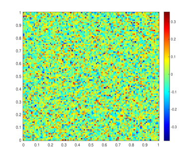
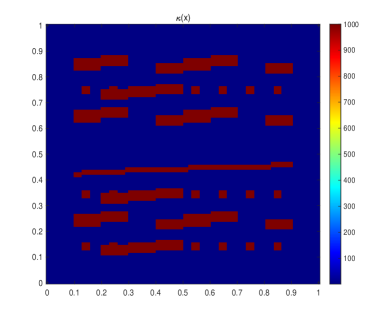
The multiscale coefficient κ(x)𝜅𝑥\kappa(x) in the above equations is depicted in Figure 3.
Refer to caption
Fig. 2: Multiscale coefficient κ(x)𝜅𝑥\kappa(x)
Refer to caption
Fig. 3: Brownian motion increment

For the stability of numerical method, we choose the stochastic full-implicit scheme to treat the temporal discretization. Then the full discretization reads as

umsk+1=umsk+Aκumsk+1Δtk+f(umsk+1)Δtk+g(umsk)ΔWk.subscriptsuperscript𝑢𝑘1𝑚𝑠subscriptsuperscript𝑢𝑘𝑚𝑠subscript𝐴𝜅subscriptsuperscript𝑢𝑘1𝑚𝑠Δsubscript𝑡𝑘𝑓subscriptsuperscript𝑢𝑘1𝑚𝑠Δsubscript𝑡𝑘𝑔subscriptsuperscript𝑢𝑘𝑚𝑠Δsubscript𝑊𝑘u^{k+1}_{ms}=u^{k}_{ms}+A_{\kappa}u^{k+1}_{ms}\Delta t_{k}+f(u^{k+1}_{ms})\Delta t_{k}+g(u^{k}_{ms})\Delta W_{k}.

The temporal is partitioned uniformly by the interval Δt=0.01Δ𝑡0.01\Delta t=0.01. We consider the Brownian motion with three different covariance coefficients Q=0.01,1,100𝑄0.011100Q=0.01,1,100 as three degenerated 𝒬𝒬\mathcal{Q}-Wiener processes. Figure 3 shows a sample of Brownian motion increment with time interval ΔtΔ𝑡\Delta t and covariance coefficients Q=1𝑄1Q=1. Since the drift term cos(u)𝑢\cos(u) is nonlinear, we get a nonlinear equation of the unknown state umsk+1superscriptsubscript𝑢𝑚𝑠𝑘1u_{ms}^{k+1}, and use Newton iteration to solve the nonlinear system. Because we focus on the performance of CEM-GMsFEM, we do not use any DEIM to reduce the nonlinear model in this subsection. We will compute the CEM-GMsFEM solutions of the deterministic and stochastic systems with the three different coefficients Q𝑄Q.

Refer to caption
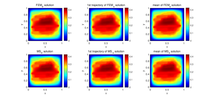
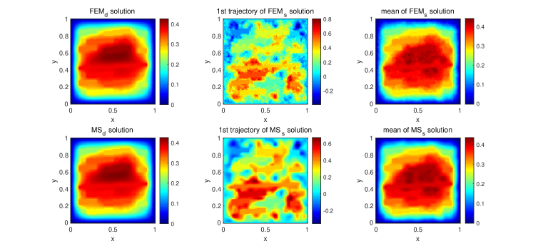
Fig. 4: Solution profiles at t=1𝑡1t=1. Top left: FEM reference solution of deterministic system; Top middle: the first trajectory of FEM reference solution of stochastic system with covariance coefficient Q=0.01𝑄0.01Q=0.01; Top right: the mean of FEM reference solution of stochastic system; Bottom: Corresponding CEM-GMsFEM solutions.

Figure 4 shows solutions of deterministic system and stochastic system at t=1𝑡1t=1. For the stochastic system, mean of solutions is approximated by averaging 100 stochastic realizations. We notice that individual behaviour (middle) and mean behaviour (right) are almost same because of a small coefficient Q𝑄Q in the stochastic system. Their solution profiles are almost the same as the solution of deterministic system.
Refer to caption
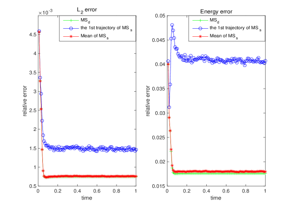
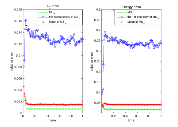
Fig. 5: Relative L2subscript𝐿2L_{2} errors (left) and relative energy errors (right) for MS solution (green ++) of deterministic problem, MS solution mean (red *) and one trajectory of MS solution (blue o𝑜o), Q=0.01𝑄0.01Q=0.01.

To evaluate the approximation accuracy, Figure 5 shows the relative L2subscript𝐿2L_{2} error and relative energy error of CEM-GMsFEM solutions. Here we take the 100 stochastic realizations to approximate expectation of stochastic solutions and reference solution is the FEM solution in fine grid. From this figure, we see that error of the individual trajectory of CEM-GMsFEM solution is much larger than the other two errors: MSdsubscriptMS𝑑\text{MS}_{d} and mean of MSssubscriptMS𝑠\text{MS}_{s}. This shows that randomness of individual path may impact on the approximation of CEM-GMsFEM because we do not consider stochastic term when we construct the basis functions of CEM-GMsFEM. Moreover, L2subscript𝐿2L_{2} error of mean of MSs is almost the same as the error of MSd, while energy error of mean of MSs is slightly larger than MSd.
Refer to caption
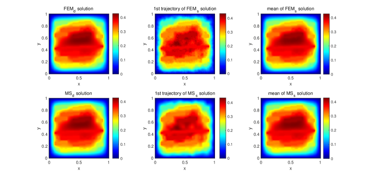
Fig. 6: Solution profiles at t=1𝑡1t=1. Top left: FEM reference solution of deterministic system; Top middle: the first trajectory of FEM reference solution of stochastic system with covariance coefficient Q=1𝑄1Q=1; Top right: the mean of FEM reference solution of stochastic system; Bottom: Corresponding CEM-GMsFEM solutions.

When the covariance coefficient Q𝑄Q of Wiener-process increases, the trajectories of SPDE may show significant difference among them. By the middle plot in Figure 6 (Q=1𝑄1Q=1), the first trajectory of the SPDE solution shows a random perturbation comparing to deterministic model solution and mean of SPDE solution. However, mean of stochastic FEM solution behaves more like FEMd solution. Figure 6 (Q=1𝑄1Q=1) shows that CEM-GMsFEM solutions approximate the FEM solutions in fine grid. As Q=0.01𝑄0.01Q=0.01 case, we illustrate L2subscript𝐿2L_{2} relative error and energy relative error of CEM-GMsFEM solutions in Figure 7 with FEM solutions as reference solutions. We see that, for the stochastic model, L2subscript𝐿2L_{2} error and energy error of the first path are both much larger than deterministic CEM-GMsFEM solution. The error of mean of CEM-GMsFEM solution to the stochastic model is also slightly larger than the error of CEM-GMsFEM solution to the deterministic model. The reason may be from Monte Carlo sampling.
Refer to caption
Fig. 7: Relative L2subscript𝐿2L_{2} errors (left) and relative energy errors (right) for MS solution (green ++) of deterministic problem, MS solution mean (red *) and one trajectory of MS solution (blue o𝑜o). Q=1𝑄1Q=1.
Refer to caption
Fig. 8: Solution profiles at t=1𝑡1t=1. Top left: FEM reference solution of deterministic system; Top middle: the first trajectory of FEM reference solution of stochastic system with covariance coefficient Q=100𝑄100Q=100; Top right: the mean of FEM reference solution of stochastic system; Bottom: Corresponding CEM-GMsFEM solutions.

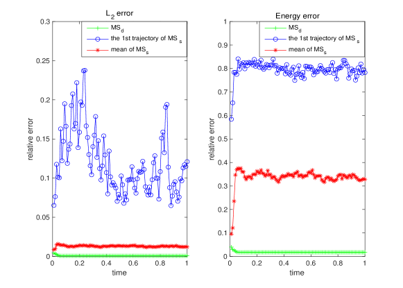
Comparing Figure 8 (Q=100𝑄100Q=100) with Figure 4 and Figure 6, we observe that the larger of the covariance coefficient Q𝑄Q leads to less accuracy of CEM-GMsFEM. This is because we construct the multiscale basis functions without considering the stochastic influence, i.e., the stochastic perturbation of the Wiener process. By Figure 9, we also see that the error of mean of CEM-GMsFEM solution is much smaller than the error of individual trajectory.
Refer to caption
Fig. 9: L2subscript𝐿2L_{2} Relative L2subscript𝐿2L_{2} errors (left) and relative energy errors (right) for MS solution (green ++) of deterministic problem, MS solution mean (red *) and one realization of MS solution (blue o𝑜o). Q=100𝑄100Q=100.
Refer to caption
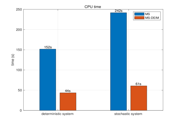
Fig. 10: CPU time for the deterministic model and the stochastic model.

Moreover, we compare the CPU time of the different methods. For the nonlinear terms, we use two different models for simulation: full-order model and DEIM reduced model. Figure 10 illustrates the CUP time for deterministic model and stochastic model using two different methods: CEM-GMsFEM (MS) and CEM-GMsFEM-DEIM (MS-DEIM). By the figure, we find that the CUP time for stochastic model is longer than the deterministic model. This is because that extra computation is required for the diffusion term of white noise. The figure also clearly shows that DEIM take much less time than Newton method for both deterministic nonlinear model and stochastic nonlinear model.

5.2 Stochastic online DEIM with CEM-GMsFEM

In this subsection, we will focus on the stochastic online DEIM incorporating with CEM-GMsFE method. The approach is referred to as Online DEIM-MS for abbreviation. We concentrate on two important problems about the approach: effect of snapshots in DEIM and performance of individual stochastic realization.

5.2.1 Effect of snapshot in offline phase and online phase of DEIM

Stochastic online DEIM needs to use snapshots from offline phase and online phase: the offline snapshots consist of mean information, and online snapshots consist of new trajectory information. Thus different choices of snapshots in offline and online phase produce the different variants of online DEIM.

In this subsection, we compute the relative errors from the online DEIM using different snapshots and explore the impact of the offline snapshots and online snapshots. Meanwhile, FEM solution and CEM-GMsFEM solution are also computed to assess the effectiveness of online DEIM-MS. For numerical simulation, we solve the following SPDE,

{du(κ(x)u)dt=cos(u)dt+(u2+2)dW(x,t)inD×(0,T],u(x,t)=0onD×(0,T],u(x,0)=sin(2πx1)sin(2πx2)inD,\left\{\begin{aligned} du-\nabla\cdot\big{(}\kappa(x)\nabla u\big{)}dt&=\cos(u)dt+(u^{2}+2)dW(x,t)\quad in\quad D\times(0,T],\\ u(x,t)&=0\quad\quad\quad\quad\quad\quad\quad\quad\quad on\quad\partial D\times(0,T],\\ u(x,0)&=\sin(2\pi x_{1})\sin(2\pi x_{2})\quad\,in\quad D,\end{aligned}\right. (44)

where the temporal partition and multiscale coefficient κ(x)𝜅𝑥\kappa(x) are chosen same as the example 5.1.

Refer to caption
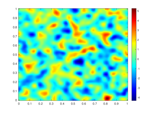
Fig. 11: A sample of the 𝒬𝒬\mathcal{Q}-Wiener process increment ΔWJ(x,t)Δsuperscript𝑊𝐽𝑥𝑡\Delta W^{J}(x,t)

In this subsection, we use a space-time 𝒬𝒬\mathcal{Q}-Wiener process described in [30]. The covariance operator 𝒬𝒬\mathcal{Q} has the eigenfunctions

ej1,j2(x)=1a1a2e2πij1x1/a1e2πij2x2/a2subscript𝑒subscript𝑗1subscript𝑗2𝑥1subscript𝑎1subscript𝑎2superscripte2𝜋𝑖subscript𝑗1subscript𝑥1subscript𝑎1superscripte2𝜋𝑖subscript𝑗2subscript𝑥2subscript𝑎2e_{j_{1},j_{2}}(x)=\frac{1}{\sqrt{a_{1}a_{2}}}\text{e}^{2\pi ij_{1}x_{1}/a_{1}}\text{e}^{2\pi ij_{2}x_{2}/a_{2}}

and eigenvalues μj1,j2=eαγj1,j2,α>0formulae-sequencesubscript𝜇subscript𝑗1subscript𝑗2superscripte𝛼subscript𝛾subscript𝑗1subscript𝑗2𝛼0{\color[rgb]{0,0,0}\mu}_{j_{1},j_{2}}=\text{e}^{-\alpha\gamma_{j_{1},j_{2}}},\,\alpha>0 and γj1,j2=j12+j22subscript𝛾subscript𝑗1subscript𝑗2superscriptsubscript𝑗12superscriptsubscript𝑗22\gamma_{j_{1},j_{2}}=j_{1}^{2}+j_{2}^{2}. The approximation of W(x,t)𝑊𝑥𝑡W(x,t) can be defined by

WJ(x,t):=j1=J1/2+1J1/2j2=J2/2+1J2/2μj1,j2ej1,j2(x)βj1,j2(t).assignsuperscript𝑊𝐽𝑥𝑡superscriptsubscriptsubscript𝑗1subscript𝐽121subscript𝐽12superscriptsubscriptsubscript𝑗2subscript𝐽221subscript𝐽22subscript𝜇subscript𝑗1subscript𝑗2subscript𝑒subscript𝑗1subscript𝑗2𝑥subscript𝛽subscript𝑗1subscript𝑗2𝑡W^{J}(x,t):=\sum_{j_{1}=-J_{1}/2+1}^{J_{1}/2}\sum_{j_{2}=-J_{2}/2+1}^{J_{2}/2}\sqrt{{\color[rgb]{0,0,0}\mu}_{j_{1},j_{2}}}e_{j_{1},j_{2}}(x)\beta_{j_{1},j_{2}}(t). (45)

We illustrate a sample of 𝒬𝒬\mathcal{Q}-Wiener process increment with J1=J2=100subscript𝐽1subscript𝐽2100J_{1}=J_{2}=100, α=0.0005𝛼0.0005\alpha=0.0005 in Figure 11.

Refer to caption
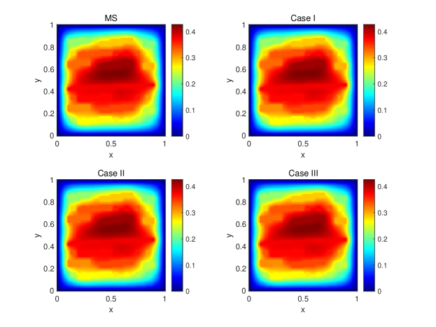
Fig. 12: Solution profiles at time t=1𝑡1t=1. Left top: CEM-GMsFEM solution; Right top: Case I; Left bottom: Case II; Right bottom: Case III.

For offline snapshots in DEIM, we compute 100100100 solutions of trajectories to get mean information. Here, we compare three different cases of offline-online. In Case I, we take mean of nonlinear evaluation in the first half time interval, i.e.,

f(u¯(x,t)),g(u¯(x,t)),(x,t)D×[0,T/2],𝑓¯𝑢𝑥𝑡𝑔¯𝑢𝑥𝑡𝑥𝑡𝐷0𝑇2f(\bar{u}(x,t)),\,g(\bar{u}(x,t)),\,(x,t)\in D\times[0,T/2],

as the mean snapshots in the offline phase, and take the nonlinear evaluation of new realization in the first half interval as new data to update the stochastic online DEIM basis matrix in the online phase. In Case II, mean of evaluation of nonlinear functions in whole time interval, i.e. f(u¯(x,t)),g(u¯(x,t)),(x,t)D×[0,T]𝑓¯𝑢𝑥𝑡𝑔¯𝑢𝑥𝑡𝑥𝑡𝐷0𝑇f(\bar{u}(x,t)),\,g(\bar{u}(x,t)),\,(x,t)\in D\times[0,T], is used in the offline phase, and online phase is the same as Case I. In Case III, offline procedure is the same as Case I, but we use the nonlinear evaluation of new trajectory in the whole time interval to update online DEIM basis in online phase. And for case III, we keep the same number of snapshots as Case I in online phase by selecting snapshots sparsely. Thus, for Case I and Case II, solutions of a new sample in the first half temporal interval demonstrate good fitness of these two techniques, while models’ predication ability are showed by the accuracy of solution in the domain D×(T/2,T]𝐷𝑇2𝑇D\times(T/2,T].

Figure 12 depicts CEM-GMsFEM solution and the Online DEIM-MS solutions associated to Case I, Case II and Case III. By the figure, the solution profiles look the same, and Online DEIM-MS is able to give a good approximation.
Refer to caption
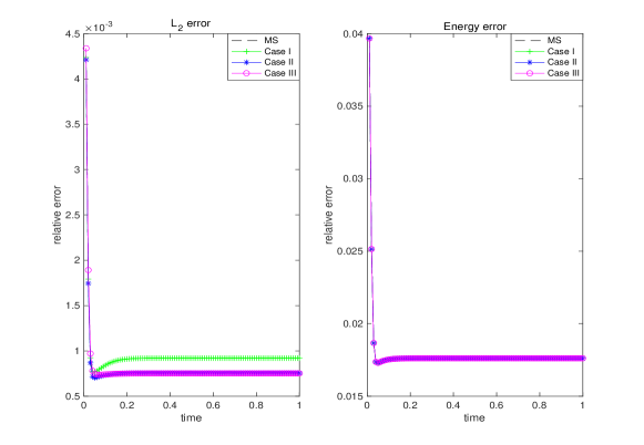
Fig. 13: Relative L2subscript𝐿2L_{2} errors (left) and relative energy errors (right) versus time t𝑡t.

The L2subscript𝐿2L_{2} errors and energy errors of above methods are showed in Figure 13. From the figure, we see that the L2subscript𝐿2L_{2} errors are almost less than 0.1%percent0.10.1\%, and the L2subscript𝐿2L_{2} error of Case I is the largest and the other two are smaller. This indicates that the use of longer time information as snapshots leads to more accurate solution. Besides, we find that CEM-GMsFEM using Newton method has the smallest error. This is consistent with our expectation. The figure shows that the errors tend to be stable as time increases. This may be because the system becomes stationary gradually.

5.2.2 Individual performance

In this numerical example, we are going to show the individual performance of online DEIM by presenting some new trajectories. We choose the same multiscale coefficient κ𝜅\kappa and 𝒬𝒬\mathcal{Q}-Wiener process as example 5.1 with noise coefficient Q=1,100𝑄1100Q=1,100. In the example, we set the nonlinear functions f(u)=2πcos(u),g(u)=u2+2formulae-sequence𝑓𝑢2𝜋𝑢𝑔𝑢superscript𝑢22f(u)=2\pi\cos(u),\,g(u)=u^{2}+2 and the initial condition u(x,0)=10sin(2πx1)sin(2πx2)𝑢𝑥0102𝜋subscript𝑥12𝜋subscript𝑥2u(x,0)=10\sin(2\pi x_{1})\sin(2\pi x_{2}). We solve the SPDE using Online DEIM (Case I in Subsection 5.2.1) combining with CEM-GMsFEM. FEM solution in fine grid is the reference solution.
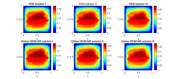
Refer to caption
Fig. 14: Solution profiles for three arbitrary trajectories, Q=1𝑄1Q=1. Top: FEM reference solutions; Bottom: Online DEIM-MS solutions (I II III are the three different trajectories).

Figure 14 shows the solution profiles of three different stochastic realizations when covarience Q=1𝑄1Q=1. The profiles of different trajectories are similar because of small covariance coefficient Q𝑄Q. The figure clearly shows that the individual performance of Online DEIM-MS solution approximates well reference solution for each trajectory.
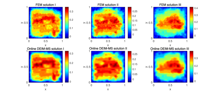
Refer to caption
Fig. 15: Solution profiles for three arbitrary trajectories, Q=100𝑄100Q=100.. Top: FEM reference solutions; Bottom: Online DEIM-MS solutions (I II III are three different trajectories).

Figure 15 depicts the solution profiles when Q=100𝑄100Q=100. Because the diffusion covarience is large, individual profiles are quite different from the three different realizations. But the Online DEIM-MS solution looks very like the FEM solutions in general. That is to say, the individual trajectory performs accurately even though the diffusion covarience becomes large.
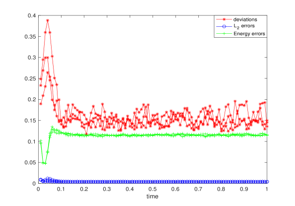
Refer to caption
Fig. 16: Relative L2subscript𝐿2L_{2} errors (blue o), relative energy errors (green +) and derivations for the three arbitrary trajectories, Q=100𝑄100Q=100.

In Figure 16, we illustrate L2subscript𝐿2L_{2} errors, energy errors and deviations of the arbitrary three realizations. Here the deviations are given by

deviation=FEM solution of arbitrary realization  mean of FEM solutions2mean of FEM solutions2.deviationsubscriptnormFEM solution of arbitrary realization  mean of FEM solutions2subscriptnormmean of FEM solutions2\text{deviation}=\sqrt{\frac{\|\text{FEM solution of arbitrary realization }-\text{ mean of FEM solutions}\|_{2}}{\|\text{mean of FEM solutions}\|_{2}}}.

Large deviation means that the problem has a very different new realization from the mean information. It is obvious in Figure 16 that the deviations are much larger than the errors. Thus large deviations and small errors indicate the good performance of Online DEIM-MS for new trajectories. One can predict how the state evolves with respect to time.

In Table 1, we make a comparison of the approximation error and the computational cost between stochastic Online DEIM and traditional DEIM, referred as Offline DEIM when these methods are applied to a single trajectory. Since their offline phases are the same, we only record the time of online phases. For Offline DEIM, the CPU time is the time of CEM-GMsFEM computation with offline-reduced nonlinear functions. But for Online DEIM, the CPU time includes both the time of online update of DEIM basis matrix and the time of MS computation with online-reduced nonlinear functions. And the relative L2subscript𝐿2L_{2} error and relative energy error are both listed in the table.

Table 1: A comparison of CPU time and relative errors.
Method CPU time(s) L2subscript𝐿2L_{2} error Energy error
MS 209.7017 5.5858×1035.5858superscript1035.5858\times 10^{-3} 7.3928×1027.3928superscript1027.3928\times 10^{-2}
Offline DEIM-MS 53.4225 7.3864×1037.3864superscript1037.3864\times 10^{-3} 7.4025×1027.4025superscript1027.4025\times 10^{-2}
Online DEIM-MS 53.4835 6.6042×1036.6042superscript1036.6042\times 10^{-3} 7.3973×1027.3973superscript1027.3973\times 10^{-2}

Table 1 shows that Online DEIM has better accuracy while it takes slightly more time than Offline DEIM. Comparing with CEM-GMsFEM without any reduction, Online DEIM is able to significantly improve the computation efficiency and keep good accuracy.

5.3 A coupled stochastic system in porous media

In this subsection, we consider a coupled system, in which SDE is coupled to a porous media equation. In this class of system, the fluid velocity is affected by the particle deposition, and the effect is described by a stochastic differential equation where the particle velocity is influenced by the fluid velocity in turn. That is to say, the particle dynamics (i.e., the stochastic differential equation in (46)) governs the permeability change. Thus the coupled system produces a stochastic porous media problem in the real world. Here is a specific system:

{u(x,t)t=(κ(x)u)+10e2vsin(u)inD×(0,T],dv(x,t)=10(vu)dt+10.1dW(t)inD×(0,T],u(x,t)=0onD×(0,T],u(x,0)=1inD,v(x,0)=2inD,\left\{\begin{aligned} \frac{\partial u(x,t)}{\partial t}&=\nabla\cdot\big{(}\kappa(x)\nabla u\big{)}+10e^{2v}\sin(u)\quad in\quad D\times(0,T],\\ dv(x,t)&=-10(v-u)dt+\frac{1}{\sqrt{0.1}}dW(t)\quad in\quad D\times(0,T],\\ u(x,t)&=0\quad\quad\quad\quad\quad\quad\quad\quad\quad\quad\quad\quad\,\,on\quad\partial D\times(0,T],\\ u(x,0)&=1\quad\quad\quad\quad\quad\quad\quad\quad\quad\quad\quad\quad\,\,in\quad D,\\ v(x,0)&=2\quad\quad\quad\quad\quad\quad\quad\quad\quad\quad\quad\quad\,\,in\quad D,\end{aligned}\right. (46)

where u𝑢u represents the fluid velocity and v𝑣v is the particle velocity. Here the permeability field κ(x)𝜅𝑥\kappa(x) is taken as the Tenth Society of Petroleum Engineers Comparative Solution Project (SPE10), which is shown in Figure 17.
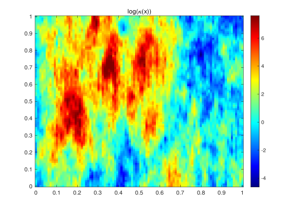
Refer to caption
Fig. 17: A permeability field (a layer from SPE10)

The model (46) describes an equation with the heterogeneous diffusion κ(x)𝜅𝑥\kappa(x), and e2vsuperscript𝑒2𝑣e^{2v} characterizes the affection by particle deposition, and 10 times of fluid velocity affects the particle velocity. We choose constant 111 and 222 as initial velocity of fluid and of particle respectively, because the particle dynamics usually occurs faster compared to fluid flow. Besides, the long time evolution of system will cause the effect that solution u𝑢u has the sharp decay to zero, and the solution becomes small after some time. To show the difference between different DEIM-MS approaches, we solve the problem in domain D=[0,1]×[0,1]𝐷0101D=[0,1]\times[0,1], with time interval t[0,0.1]𝑡00.1t\in[0,0.1]. In this example, we divide the time into N=100𝑁100N=100 intervals with step size Δt=0.001Δ𝑡0.001\Delta t=0.001, and compute 100100100 trajectories’ solutions to get mean snapshots, and Q=0.01𝑄0.01Q=0.01 for the Wiener process W(t)𝑊𝑡W(t).

We solve the coupled system sequentially (the semilinear PDE is solved after SDE), and we use drift-implicit Milstein scheme to solve SDE, while PDE is solved by four different methods : MS, Offline DEIM-MS, Online DEIM-MS and FEM in fine grid. We compute Offline DEIM-MS solution by the reduced model constructed in the offline phase where we utilize only the snapshots of nonlinear function e2vsin(u)superscript𝑒2𝑣𝑢e^{2v}\sin(u) along mean of offline trajectories, while Online DEIM-MS solution is computed by Case I in Section 5.2.
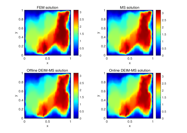
Refer to caption
Fig. 18: Solution profiles of fluid velocity u𝑢u

Figure 18 shows the profiles of fluid velocity u𝑢u. By the figure, Online DEIM-MS solution at time t=0.055𝑡0.055t=0.055 is more close to the MS and FEM solution, while Offline DEIM-MS solution obviously differs from reference solution in some locations. This shows that Online DEIM-MS is better than Offline DEIM-MS for prediction.
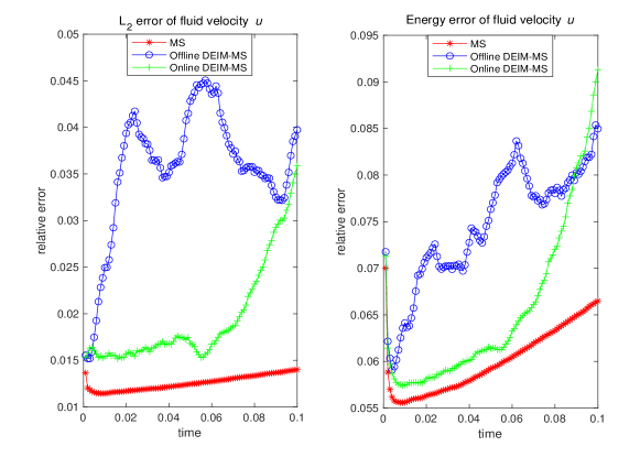
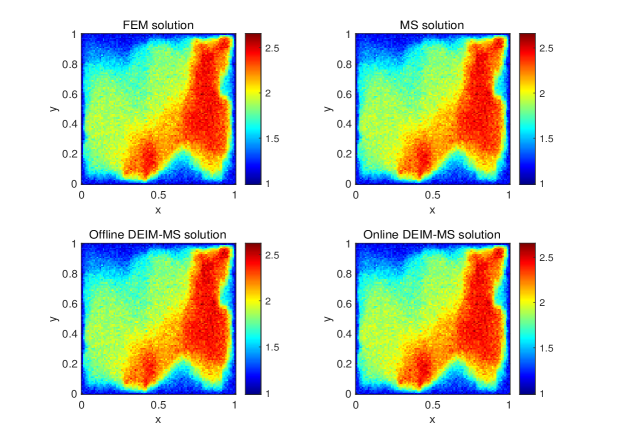
Refer to caption
Fig. 19: Relative L2subscript𝐿2L_{2} errors (left) and energy errors (right) of fluid velocity u𝑢u versus time t𝑡t
Refer to caption
Fig. 20: Solution profiles of particle velocity v𝑣v at t=0.055𝑡0.055t=0.055.

Figure 19 shows the relative errors versus time. By the figure, we observe that the error of MS solution is the smallest. This coincides with the previous examples. In the offline phase,mean information in the first half time interval is used to construct the snapshots, compute the DEIM basis matrix and interpolation matrix. This yields a reduced model using Offline DEIM and Online DEIM. Moreover, for Online DEIM, we also utilize the data of new path to update the basis matrix in the online phase. Therefore, for t[0,T/2)𝑡0𝑇2t\in[0,T/2), where T=0.1𝑇0.1T=0.1, Online DEIM produces the fitness of system evolution, while for t(T/2,T]𝑡𝑇2𝑇t\in(T/2,T], Online DEIM can predict the propogation of system. But the prediction may perform well only in a short time interval, since the correlation will decay with the elapse of time. Comparing the error curve in Figure 19, we see that Online DEIM-MS is much more precise than Offline DEIM-MS for t[0,T/2)𝑡0𝑇2t\in[0,T/2). For t(T/2,T]𝑡𝑇2𝑇t\in(T/2,T], the error of Online DEIM-MS increases over time as expected. Although the error of Online DEIM-MS grows in the later half interval, it is still much less than the error of Offline DEIM-MS. This implies that the prediction of Online DEIM is better than Offline DEIM. This verifies the accuracy of fitness and forecast of Online DEIM-MS approach.

In Figure 20, we give the profiles of particle velocity v𝑣v at time t=0.055𝑡0.055t=0.055. We note that v𝑣v is solved by plugging u𝑢u into the stochastic equation. The solution u𝑢u is computed by four different methods: FEM in fine grid, MS, Offline DEIM-MS and Online DEIM-MS. Different solutions of u𝑢u lead to different solutions of v𝑣v because they are coupled each other. By the figure, we find that the solution profiles are very close to each other. Comparing with Figure 18,the particle velocity v𝑣v is not as smooth as the fluid velocity, due to the direct impact from Brownian motion. However, the particle and the fluid velocity have the similar pattern because the particle dynamics and the fluid dynamics interact on each other. We see that, for arbitrary t[0,T]𝑡0𝑇t\in[0,T], the error of Offline DEIM-MS solution is larger than that of Online DEIM-MS. The trend of error of particle velocity is consistent with the error of fluid velocity.
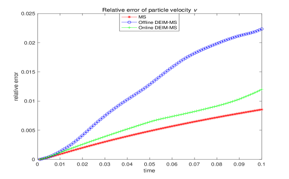
Refer to caption
Fig. 21: Relative L2subscript𝐿2L_{2} errors of the particle velocity v𝑣v versus time t𝑡t

6 Conclusion

We presented a stochastic online model reduction approach for multiscale nonlinear stochastic parabolic PDEs. Multiscales and nonlinearity significantly impact on the computation using traditional FEM in a fine grid. CEM-GMsFEM and DEIM can substantially improve the computation efficiency. We have carried out the error analysis of CEM-GMsFEM for the nonlinear stochastic PDEs. However, the semi-discrete system is still nonlinear in a high-dimensional space by CEM-GMsFEM. In order to overcome this challenge, we proposed the stochastic online DEIM method, which used the offline mean information and the online trajectory snapshots. The online DEIM significantly reduced the computation complexity for the nonlinear system. By incorporating the stochastic online DEIM with CEM-GMsFEM, we developed a stochastic multiscale model reduction method: Online DEIM-MS. This method showed superiority in prediction compared with Offline DEIM approach. We presented a few numerical examples from the porous media application to show effectiveness of the stochastic online model reduction method.

References

  • [1] J. Aarnes, Y. Efendiev and L. Jiang, Mixed multiscale finite element methods using limited global information, Multiscale Modeling & Simulation, 7(2)(2008), pp.655–676.
  • [2] T. Arbogast, K. Boyd, Subgrid upscaling and mixed multiscale finite elements, SIAM Journal on Numerical Analysis, 44(3)(2006), pp.1150–1171.
  • [3] T. Arbogast, G. Pencheva, M. Wheeler and I. Yotov, A multiscale mortar mixed finite element method, Multiscale Modeling & Simulation, 6(1)(2007), pp.319-346.
  • [4] A. Brahim, Homogenized behavior of two-phase flows in natured reservoirs with uniform fractures distribution, Transport in Porous Media, 10(1993), pp.43-56.
  • [5] H. Bessaih, Y. Efendiev and R. F. Maris, Stochastic homogenization for a diffusion-reaction model, Discrete & Continuous Dynamical Systems, 39(9)(2019), pp. 5403-5429.
  • [6] H. Bessaih, Y. Efendiev and F. Maris, Homogenization of Brinkman flows in heterogeneous dynamic media, Stochastic Partial Differential Equations: Analysis and Computations, 3(2015), pp.479-505.
  • [7] M. Barrault, Y. Maday, N. C. Nguyen and A. T. Patera, An ‘empirical interpolation’ method: application to efficient reduced-basis discretization of partial differential equations, Comptes Rendus Mathematique, 339(9)(2004), pp.667-672.
  • [8] C.-C. Chu, I.G. Graham, T.-Y. Hou, A new multiscale finite element method for high-contrast elliptic interface problems, Mathematics of Computation, 79(272)(2010), pp.1915-1955.
  • [9] E. T. Chung, Y. Efendiev and T. Y. Hou, Adaptive multiscale model reduction with generalized multiscale finite element methods, Journal of Computational Physics, 320(2016), pp.69-95.
  • [10] E. T. Chung, Y. Efendiev and W. T. Leung, Constraint Energy Minimizing Generalized Multiscale Finite Element Method, Computer Methods in Applied Mechanics and Engineering, 339(2018), pp.298-319.
  • [11] F. Chen, E. Chung and L. Jiang, Least-squares mixed generalized multiscale finite element method, Computer Methods in Applied Mechanics and Engineering, 311(2016), pp.764-787.
  • [12] S. Chaturantabut, D. C. Sorensen,Nonlinear Model Reduction via Discrete Empirical Interpolation, SIAM Journal on Scientific Computing, 32(5)(2010), pp.2737-2764.
  • [13] M. Drohmann, B. Haasdonk and M. Ohlberger, Reduced basis approximation for nonlinear parametrized evolution equations based on empirical operator interpolation, SIAM Journal on Scientific Computing, 34(2)(2012), pp.A937-A969.
  • [14] J. Duan, W. WANG , Effective Dynamics of Stochastic Partial Differential Equations, Academic Press(2014), Boston.
  • [15] W. E, B. Engquist, Heterogeneous multiscale methods, Communications in Mathematical Sciences, 1(1)(2003), pp.87-132.
  • [16] Y. Efendiev, J. Galvis and T. Hou, Generalized multiscale finite element methods, Journal of Computational Physics, 251(2013), pp.116-135.
  • [17] Y. Efendiev, J. Galvis and X. Wu, Multiscale finite element methods for high-contrast problems using local spectral basis functions, Journal of Computational Physics, 230(4)(2011), pp.937-955.
  • [18] R. G. Gordeev, The existence of a periodic solution in a tide dynamics problem, Journal of Soviet Mathematics, 6(1–4)(1976).
  • [19] L. Gawarecki, V. Mandrekar, Stochastic Differential Equations in Infinite Dimensions. with Applications to Stochastic Partial Differential Equations, Probability and Its Applications(2011), Springer, Berlin, Heidelberg.
  • [20] T. Hughes, G. Feijoo, L. Mazzei and J. Quincy, The variational multiscale method – a paradigm for computational mechanics, Computer Methods in Applied Mechanics and Engineering, 166(1-3)(1998), pp.3-24.
  • [21] O. Iliev, R. Lazarov and J. Willems, Variational multiscale finite element method for flows in highly porous media, Multiscale Modeling & Simulation, 9(4)(2011), pp. 135-1372.
  • [22] R. Juanes, A variational multiscale finite element method for multiphase flow in porous media, Finite Elements in Analysis and Design, 41(7–8)(2005), pp.763-777.
  • [23] P. Jenny, S. Lee, H. Tchelepi, Multi-scale finite volume method for elliptic problems in subsurface flow simulation, Journal of Computational Physics, 187(1)(2003), pp.47-67.
  • [24] L. Jiang, Y. Efendiev and G. Victor, Multiscale methods for parabolic equations with continuum spatial scales, Discrete Contin. Dyn. Syst. Ser. B, 8 (2007), pp. 833–859.
  • [25] R. Kruse, Strong and Weak Approximation of Semilinear Stochastic Evolution Equations, Lecture Notes in Mathematics, 2093(2014), Springer International Publishing.
  • [26] P. E. Kloeden, S. Shott, Linear-implicit strong schemes for Ito^^𝑜\hat{o}-Galerkin approximations of stochastic PDEs, Journal of Applied Mathematics and Stochastic Analysis, 14(1)(2001), pp.47-53.
  • [27] D. Kulasiri, W. Verwoerd, Stochastic Dynamics: Modeling Solute Transport in Porous Media, North-Holland Series in Applied Mathematics and Mechanics, 44(2002), North Holland.
  • [28] V. K. Kalantarov, S. Zelik, Smooth attractors for the Brinkman–Forchheimer equations with fast growing nonlinearities, Communications on Pure & Applied Analysis, 11(5)(2012), pp.2037-2054.
  • [29] M. Li, E. T. Chung and L. Jiang ,A Constraint energy minimizing generalized multiscale finite element method for parabolic equations,Multiscale Modeling and Simulation, 17 (3) (2019), pp. 996-1018.
  • [30] G. J. Lord, C. E. Powell and T. Shardlow, An Introduction to Computational Stochastic PDEs., Cambridge Texts in Applied Mathematics(2014), Cambridge University Press, Cambridge.
  • [31] G. J. Lord, A. Tambue, Stochastic exponential integrators for the finite element discretization of SPDEs for multiplicative & additive noise, IMA Journal of Numerical Analysis, 33(2)(2013), pp.515-543.
  • [32] A. Malqvist and D. Peterseim, Localization of elliptic multiscale problems, Mathematics of Computation, 83 (290) (2014), pp. 2583-2603.
  • [33] J. D. Mukam, A. Tambue, Strong Convergence Analysis of the Stochastic Exponential Rosenbrock Scheme for the Finite Element Discretization of Semilinear SPDEs Driven by Multiplicative and Additive Noise, Journal of Scientific Computing, 74(2018), pp.937-978.
  • [34] D. A. Nield, A. Bejan, Convection in Porous Media-Forth Edition, Springer(2013), New York.
  • [35] B. Øksendal, Stochastic Differential Equations: An Introduction with Applications-Fifth Edition, Springer(2003), Berlin, Heidelberg.
  • [36] B. Peherstorfer, K. Willcox, Online adaptive model reduction for nonlinear systems via low-rank updates, SIAM Journal on Scientific Computing, 37(4)(2015), pp.A2123-A2150.
  • [37] G. D. Prato, J. Zabczyk, Stochastic Equations in Infinite Dimensions, Encyclopedia of Mathematics and its Applications(2008), Cambridge University Press, Cambridge.
  • [38] S. Peszat, J. Zabczyk, Stochastic Partial Differential Equations with Le´´𝑒\acute{e}vy Noise. An Evolution Equation Approach, Encyclopedia of Mathematics and Its Applications, 113(2007), Cambridge University Press, Cambridge.
  • [39] B. Straughan, Stability and Wave Motion in Porous Media, Applied Mathematical Sciences, 165(2008), Springer, New York.
  • [40] A. Tambue, J. D. Mukam, Magnus-type integrator for non-autonomous SPDEs driven by multiplicative noise, Discrete & Continuous Dynamical Systems, 40(8)(2020), pp.459-4624.
  • [41] M. Wheeler, G. Xue, I. Yotov, A multiscale mortar multipoint flux mixed finite element method, ESAIM: Mathematical Modelling and Numerical Analysis, 46(4)(2012), pp.759-796.
  • [42] S. Zhang, X. Guan and L. Jiang, Convergence analysis of constraint energy minimizing generalized multiscale finite element method for a linear stochastic parabolic partial differential equation driven by additive noises, Journal of Computational and Applied Mathematics, 389 (2021), Paper No. 113328
  • [43] Z. Zhang, G. E. Karniadakis, Numerical Method for Stochastic Partial Differential Equations with White Noise, Applied Mathematical Sciences, 196(2017), Springer International Publishing.