Calibrating distribution models from PELVE

Abstract

The Value-at-Risk (VaR) and the Expected Shortfall (ES) are the two most popular risk measures in banking and insurance regulation. To bridge between the two regulatory risk measures, the Probability Equivalent Level of VaR-ES (PELVE) was recently proposed to convert a level of VaR to that of ES. It is straightforward to compute the value of PELVE for a given distribution model. In this paper, we study the converse problem of PELVE calibration, that is, to find a distribution model that yields a given PELVE, which may either be obtained from data or from expert opinion. We discuss separately the cases when one-point, two-point, $n$-point and curve constraints are given. In the most complicated case of a curve constraint, we convert the calibration problem to that of an advanced differential equation. We apply the model calibration techniques to estimation and simulation for datasets used in insurance. We further study some technical properties of PELVE by offering a few new results on monotonicity and convergence.

Keywords: Value-at-Risk, Expected Shortfall, risk measures, heavy tails, advanced differential equation.

1 Introduction

Value-at-Risk (VaR) and Expected Shortfall (ES, also known as TVaR and CVaR) are the most widely used risk measures for regulation in finance and insurance. The former has gained its popularity due to its simplistic approach toward risk as the risk quantile, and the second one is perceived to be useful as a modification of VaR with more appealing properties, such as tail-sensitivity and subadditivity, as studied in the seminal work of Artzner et al. (1999).

In the Fundamental Review of the Trading Book (FRTB), the Basel Committee on Banking Supervision (BCBS (2019)) proposed to replace VaR at 1% confidence with ES with a 2.5% confidence interval for the internal model-based approach. The main reason, as mentioned in the FRTB, was that $\mathrm{ES}$ can better capture tail risk; see Embrechts et al. (2018) for a concrete risk sharing model where tail risk is captured by ES and ignored by VaR. On the other hand, VaR also has advantages that ES does not have, such as elicitability (e.g., Gneiting (2011) and Kou and Peng (2016)) or backtesting tractability (e.g., Acerbi and Székely (2014)), and the two risk measures admit different axiomatic foundations (see Chambers (2009) and Wang and Zitikis (2021)). We refer to the reviews of Embrechts et al. (2014) and Emmer et al. (2015) for general discussions on VaR and ES, and McNeil et al. (2015) for a standard treatment on risk management including the use of VaR and ES. The technical contrasts of the two risk measures and their co-existence in regulatory practice give rise to great interest from both researchers and practitioners to explore the relationship between them.

To understand the balancing point of VaR and ES during the transition in the FRTB, Li and Wang (2022) proposed the Probability Equivalent Level of VaR-ES (PELVE). The value of PELVE is the multiplier to the tail probability when replacing VaR with ES such that the capital calculation stays unchanged. More precisely, the PELVE of $X$ at level $\varepsilon$ is the multiplier $c$ such that $\mathrm{ES}_{c\varepsilon}(X)=\mathrm{VaR}_{\varepsilon}(X)$; such $c$ uniquely exists under mild conditions. For instance, if $\mathrm{VaR}_{1\%}(X)=\mathrm{ES}_{2.5\%}(X)$ for a future portfolio loss $X$, then PELVE of $X$ at probability level 0.01 is the multiplier $2.5$. In this case, replacing $\mathrm{VaR}_{1\%}$ with $\mathrm{ES}_{2.5\%}$ in FRTB does not have much effect on the capital requirement for the bank bearing the loss $X$. Instead, if $\mathrm{ES}_{2.5\%}(X)>\mathrm{VaR}_{1\%}(X)$, then the bank has a larger capital requirement under the new regulatory risk measure; this is often the case for financial assets and portfolios as shown by the empirical studies in Li and Wang (2022). The PELVE enjoys many convenient properties, and it has been extended in a few ways. In particular, Fiori and Rosazza Gianin (2023) defined generalized PELVE by replacing $\mathrm{VaR}$ and $\mathrm{ES}$ with another pair of monotone risk measures $(\rho,\tilde{\rho})$, and Barczy et al. (2022) extended PELVE by replacing ES with a higher-order ES.

For a given distribution model or a data set, its PELVE can be computed or estimated in a straightforward manner. As argued by Li and Wang (2022), the PELVE for a small $\varepsilon$ may be seen as a summarizing index measuring tail heaviness in a non-limit sense. As such, one may like to generate models for a given PELVE, in a way similar to constructing models for other given statistical information; see e.g., Embrechts et al. (2002, 2016) for constructing multivariate models with a given correlation or tail-dependence matrix. Such statistical information may be obtained either from data or from expert opinion, but there is no a priori guarantee that a corresponding model exists. Since PELVE involves a parameter $\varepsilon\in(0,1)$, its information is represented by a curve. The calibration problem, that is, to find a distribution model for given PELVE values or a given PELVE curve, turns out to be highly non-trivial, and it is the main objective of the current paper.

From now on, suppose that we receive some information on the PELVE of a certain random loss from an expert opinion, and we aim to build a distribution model consistent with the supplied information. Since PELVE is location-scale invariant, such a distribution, if it exists, is not unique.

The calibration problem is trivial if we are supplied with only one point on the PELVE curve. As the PELVE curve of the generalized Pareto distribution is a constant when the PELVE is well defined, we can use the generalized Pareto distribution to match the given PELVE value, which has a tail index implied from the expert opinion. The calibration problem becomes more involved if we are supplied with two points on the PELVE curve, because the value of the PELVE at two different probability levels interact with each other. The situation becomes more complicated as the number of points increases, and we further turn to the problem of calibration from a fully specified PELVE curve. Calibrating distribution from the PELVE curve can be reformulated as solving for a function $f$ via the integral equation $\int_{0}^{y}f\left(s\right)\mathrm{d}s=yf\left(z\left(y\right)y\right)$, where the curve $z$ is computed from the PELVE curve. This integral equation can be further converted to an advanced differential equation (see Bellman and Cooke (1963)). For the case that $z$ is a constant curve, we can explicitly obtain all solutions for $f$. We find other distributions that also have constant PELVE curves other than the simple ones with a Pareto or exponential distribution. As a consequence, a PELVE curve does not characterize a unique location-scale family of distributions; this provides a negative answer to a question posed by Li and Wang (2022, Section 7, Question (iv)). For general function $z$, we develop a numerical method to compute $f$.

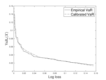
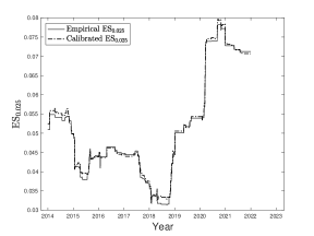
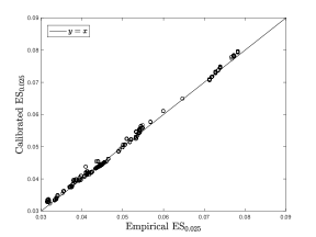
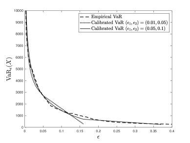
The calibrated distribution can be used to estimate the value of other risk measures such as VaR and ES at different levels. We illustrate by an empirical example that two points of PELVE give a quite good summary of the tail distribution of risk. Daily log-losses (negative log-returns) of Apple (AAPL) from Yahoo Finance are collected for the period from January 3, 2012 to December 31, 2021 within total of 2518 observations. We calculate the empirical PELVE at levels 0.01 and 0.05 using the empirical PELVE estimator provided by Li and Wang (2022, Section 5) with a moving window of 500 trading days. For each pair of two points of PELVE at levels 0.01 and 0.05, we produce a quantile curve from the two empirical PELVE points by our calibration model in Section 3.2, which is scaled such that $\mathrm{VaR}_{0.01}$ and $\mathrm{VaR}_{0.05}$ are equal to their empirical values. Figure 1 presents the empirical and calibrated quantile curves on December 31, 2021 using 500 trading days prior to that date. The two quantile curves are close to each other, with our calibrated curve being more smooth. We also report the values of $\mathrm{ES}_{0.025}$ of the calibrated distribution, which we call the calibrated $\mathrm{ES}_{0.025}$, and compare it with empirical $\mathrm{ES}_{0.025}$. The left panel of Figure 2 shows the curves of empirical and calibrated $\mathrm{ES}_{0.025}$. In the right panel of Figure 2, we create a scatter plot using empirical and calibrated $\mathrm{ES}_{0.025}$. Both figures show that the empirical and calibrated $\mathrm{ES}_{0.025}$ curves are quite close.

Figure 1: Empirical $\mathrm{VaR}$ and calibrated $\mathrm{VaR}$

Figure 2: Empirical $\mathrm{ES}_{0.05}$ and calibrated $\mathrm{ES}_{0.05}$

To further enrich the theory of PELVE, we study a few technical properties of PELVE, such as monotonicity and convergence as the probability level goes to 0. A decreasing PELVE indicates a relatively larger impact of $\mathrm{ES}$ in risk assessment than $\mathrm{VaR}$ moving towards the tail. As we will see, while for the most known parametric distributions the PELVE is decreasing, there exist some examples at some risk levels it is not decreasing. This means that for those examples $\mathrm{VaR}$ becomes a stricter risk measure when moving towards the tail. To obtain conditions for monotonicity, we define the dual PELVE by moving the multiplier $c$ from the $\mathrm{ES}$ side to the $\mathrm{VaR}$ side. PELVE can be seen as a functional measure of tail heaviness in the sense that a heavier-tailed distribution has a higher PELVE curve (Li and Wang (2022, Theorem 1)). The hazard rate, on the other hand, is another functional measure of tail heaviness. We show that the PELVE is decreasing (increasing) if the inverse of the hazard rate is convex (concave). Monotonicity also leads to conditions for the PELVE to have a limit at the tail, which from the risk management perspective, identifies the ultimate relative positions of $\mathrm{ES}$ and $\mathrm{VaR}$ in the tail region. From a mathematical perspective, the limit of PELVE at $0$ allows us to extend the domain of PELVE to include $0$ as a measure of tail heaviness.

The rest of this paper is organized as follows. Section 2 introduces the background and examples of the PELVE. In Section 3 we calibrate a distribution from finitely many points in the PELVE curve. Section 4 calibrates the distribution from given PELVE curves, where we give a class of explicit solutions for constant PELVE functions and numerical solutions for general PELVE functions. In Section 5, we study the monotonicity and convergence of the PELVE. Section 6 presents two examples of the model calibration techniques applied to datasets used in insurance. A conclusion is given in Section 7. Some technical proofs of results in Sections 3, 4 and 5 are provided in the Appendices.

2 Definitions and background

Let us consider an atomless probability space $\left(\Omega,\mathcal{F},\mathbb{P}\right)$, where $\mathcal{F}$ is the set of the measurable sets and $\mathbb{P}$ is the probability measure. Let $L^{1}$ be the set of integrable random variables, i.e., $L^{1}=\{X:\mathbb{E}[|X|]<\infty\}$, where $\mathbb{E}$ is the expectation with respect to $\mathbb{P}$.

We first define $\mathrm{VaR}$ and $\mathrm{ES}$ in $L^{1}$, the two most popular risk measures. The $\mathrm{VaR}$ at probability level $p\in(0,1)$ is defined as

$$\mathrm{VaR}_{p}(X)=\inf\{x\in\mathbb{R}:\mathbb{P}(X\leqslant x)\geqslant 1-p\}=F^{-1}(1-p),~{}~{}~{}~{}X\in L^{1},$$ (1)

where $F$ is the distribution of $X$. The $\mathrm{ES}$ at probability level $p\in[0,1)$ is defined as

$$\mathrm{ES}_{p}(X)=\frac{1}{p}\int_{0}^{p}\mathrm{VaR}_{q}(X)\mathrm{d}q,~{}~{}~{}~{}X\in L^{1}.$$

Note that we use the “small $\alpha$” convention for $\mathrm{VaR}$ and $\mathrm{ES}$, which is different from Liu and Wang (2021). Let $\mathrm{VaR}_{0}(X)=\mathrm{ES}_{0}(X)=\mathrm{ess\mbox{-}sup}(X)$ and $\mathrm{VaR}_{1}(X)=\mathrm{ess\mbox{-}inf}(X)$. We have that $\mathrm{ES}_{1}(X)$ is the mean of $X$. We will also call $p\mapsto\mathrm{VaR}_{p}(X)$ the quantile function of $X$, keeping in mind that in our convention this function is decreasing.

For $\varepsilon\in(0,1)$, the PELVE at level $\varepsilon$, proposed by Li and Wang (2022), is defined as

$$\Pi_{X}(\varepsilon)=\inf\left\{c\in[1,1/\varepsilon]:\mathrm{ES}_{c\varepsilon}(X)\leqslant\mathrm{VaR}_{\varepsilon}(X)\right\},\quad X\in L^{1},$$

where $\inf(\varnothing)=\infty$. Li and Wang (2022) used $\Pi_{\varepsilon}(X)$ for our $\Pi_{X}(\varepsilon)$, and our choice of notation is due to the fact that the curve $\varepsilon\to\Pi_{X}(\varepsilon)$ is the main quantity of interest in this paper.

The PELVE of $X$ is finite if and only if $\mathrm{VaR}_{\varepsilon}(X)\geqslant\mathbb{E}[X]$. The value of the PELVE is the multiplier $c$ such that $\mathrm{ES}_{c\varepsilon}(X)=\mathrm{VaR}_{\varepsilon}(X).$ If $\mathrm{VaR}_{p}(X)$ is not a constant for $p\in(0,\varepsilon]$, then the PELVE is the unique solution for the multiplier. By Theorem 1 in Li and Wang (2022), the PELVE is location-scale invariant. The distribution with a heavy tail will have a higher PELVE value.

If $X$ is a normal distributed random variable and $\varepsilon=1\%$, we have $\Pi_{X}(\varepsilon)\approx 2.5$. It means that $\mathrm{ES}_{2.5\%}(X)\approx\mathrm{VaR}_{1\%}(X)$. That is, the replacement suggested by BCBS is fair for normally distributed risks. In other words, a higher PELVE will result in a higher capital requirement after the replacement.

In this paper, we are generally interested in the question of which distributions have a specified or partially specified PELVE curve. We first look at a few simple examples.

Example 1 (Constant PELVE).

We first list some distributions that have constant PELVE curves. From the definition of the PELVE, we know that the PELVE should be larger than 1. As we can see from Table 1, the PELVE for the generalized Pareto distribution takes values on $(1,\infty)$. For $X\sim\text{GPD}(\xi)$, we have $1<\Pi_{X}(\varepsilon)<e$ when $\xi<0$, $\Pi_{X}(\varepsilon)=e$ when $\xi=0$ and $\Pi_{X}(\varepsilon)>e$ when $\xi>0$. Furthermore, if $X$ follows the point-mass distribution $\delta_{c}$ or the Bernoulli distribution, we have $\Pi_{X}(\varepsilon)=1$.

Table 1: Example of constant PELVE

Distribution	Distribution or probability function of $X$	$\Pi_{X}(\varepsilon)$
$\delta_{c}$	$\mathbb{P}(X=c)=1$	$\Pi_{X}(\varepsilon)=1$ for $\varepsilon\in(0,1)$
$\mathrm{B}(1,p)$	$\mathbb{P}(X=1)=p$ and $\mathbb{P}(X=0)=1-p$	$\Pi_{X}(\varepsilon)=1$ for $\varepsilon\in(0,p)$
$\mathrm{U}(0,1)$	$F(t)=t$ for $t\in(0,1)$	$\Pi_{X}(\varepsilon)=2$ for $0<\varepsilon<1/2$
$\text{EXP}(\lambda)$	$F(t)=1-\exp(-\lambda t),~{}~{}\lambda>0$	$\Pi_{X}(\varepsilon)=e$ for $0<\varepsilon<1/e$
$\text{GPD}(\xi)$1	$F(x)=\left\{\begin{aligned} &1-\left(1+\xi x\right)^{-\frac{1}{\xi}}~{}~{}~{}&\xi\neq 0\\ &1-\exp(-x)~{}~{}~{}&\xi=0\end{aligned}\right.$	$\Pi_{X}(\varepsilon)=(1-\xi)^{-\frac{1}{\xi}}$ for $0<\varepsilon<(1-\xi)^{\frac{1}{\xi}}$

• The distribution $\text{GPD}(\xi)$ is called the standard generalized Pareto distribution. As $\mathbb{E}[X]<\infty$ when $\xi<1$, the PELVE exists only when $\xi<1$. The support of $\text{GPD}(\xi)$ is $[0,\infty)$ when $\xi>0$ and $[0,-\frac{1}{\xi}]$ when $\xi<0$. When $\xi=0$, the $\text{GPD}(\xi)$ is exactly exponential distribution with $\lambda=1/\sigma$. There is a three-parameter $\text{GPD}(\mu,\sigma,\xi)$, which is a location-scale transform of standard GPD. Therefore, $\text{GPD}(\mu,\sigma,\xi)$ has the same PELVE as $\text{GPD}(\xi)$.

Example 2.

Here we present some non-constant PELVE examples. We write $\mathrm{t}(v)$ for the t-distribution with parameter $(0,1,v)$, and $\mathrm{LN}(\sigma)$ for the log-normal distribution with parameter $(0,\sigma^{2})$.

Figure 3: PELVE for normal distribution, t-distribution and lognormal distribution

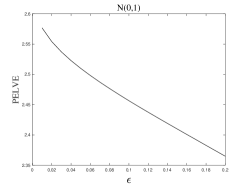
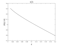
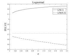
As we can see, for normal distribution and t-distribution, the PELVE curve is decreasing as $\varepsilon$ increasing. The monotonicity of the PELVE of the lognormal distribution depends on the value of $\sigma$. The monotonicity of the PELVE will be further discussed in Section 5. For more PELVE examples, see Li and Wang (2022).

3 Calibration from finite-point constraints

In this section, we discuss the calibration problem when some points of the PELVE are given. We will focus on the case where one point or two points on the PELVE curve are specified, for which we can explicitly construct a corresponding quantile function.

We first note that the calibrated distribution is not unique. For example, if we are given $\Pi_{X}(0.01)=2.5$, we can assume the distribution of $X$ is the Normal distribution or the generalized Pareto distribution with tail parameter $\xi$ satisfying $(1-\xi)^{-1/\xi}=2.5$ from Table 1. Therefore, the distributions obtained in our results are only some possible choices, which we choose to have a generalized Pareto tail, as Pareto tails are standard in risk management applications.

3.1 Calibration from a one-point constraint

Based on Table 1, we can calibrate the distribution for $X$ from one given PELVE point $(\varepsilon_{1},c_{1})$ such that $\Pi_{X}({\varepsilon_{1}})=c_{1}$. A simple idea is to take the generalized Pareto distribution when $c_{1}>1$ and $\delta_{c}$ when $c_{1}=1$. We summarize the idea in the following Proposition.

Proposition 1.

Let $\varepsilon_{1}\in(0,1)$ and $c_{1}\in[1,\infty)$ such that $c_{1}\varepsilon_{1}\leqslant 1$. If $c_{1}>1$, let $\xi\in\mathbb{R}$ such that $(1-\xi)^{-\frac{1}{\xi}}=c_{1}$. Then, $X\sim\text{GPD}(\xi)$ has $\Pi_{X}({\varepsilon_{1}})=c_{1}$. If $c_{1}=1$, then $X=k$ for some constant $k\in\mathbb{R}$ has $\Pi_{X}({\varepsilon_{1}})=c_{1}$.

The proof can be directly derived from Table 1 and it is omitted. By Proposition 1, if we have the value of PELVE at point $\varepsilon_{1}$, we can find a distribution of $X$ which has the same PELVE value at $\varepsilon_{1}$. If we also have the value of $\mathrm{VaR}$ at $\varepsilon_{1}$, we can determine the scale parameter ($\sigma$) for the GPD distribution or the value of $k$ to match the value of $\mathrm{VaR}$. For Table 1, we can see that the calibrated generalized Pareto distribution can also serve as a solution for a more prudent condition $\Pi_{X}(\varepsilon)\geqslant c_{1}$ when $\varepsilon\in(0,\varepsilon_{1})$.

3.2 Calibration from a two-point constraint

The calibration problem would be much more difficult when we are given two points of the PELVE curve. Given two points $(\varepsilon_{1},c_{1})$ and $(\varepsilon_{2},c_{2})$ such that $\varepsilon_{1}<\varepsilon_{2}$, we want to find a distribution for $X\in L^{1}$ such that $\Pi_{X}({\varepsilon_{1}})=c_{1}$ and $\Pi_{X}(\varepsilon_{2})=c_{2}$. Nevertheless, the choices of $(\varepsilon_{1},c_{1})$ and $(\varepsilon_{2},c_{2})$ are not arbitrary. First, we need $1\leqslant c_{1}\leqslant 1/\varepsilon_{1}$ and $1\leqslant c_{2}\leqslant 1/\varepsilon_{2}$ by the definition of the PELVE. Then, we will show that the value of $c_{2}$ will be restricted if $(\varepsilon_{1},c_{1})$ and $\varepsilon_{2}$ are given.

Lemma 1.

For any $X\in L^{1}$, let $\varepsilon_{1},\varepsilon_{2}\in(0,1)$ be such that $\mathbb{E}[X]\leqslant\mathrm{VaR}_{\varepsilon_{2}}(X)$ and $\varepsilon_{1}<\varepsilon_{2}$. Then, we have $\varepsilon_{1}\Pi_{X}(\varepsilon_{1})\leqslant\varepsilon_{2}\Pi_{X}(\varepsilon_{2})$.

By Lemma 1, for given $\varepsilon_{1},\varepsilon_{2}$ and $c_{1}$, the value of $c_{2}$ is bounded below by both 1 and ${c_{1}\varepsilon_{1}}/{\varepsilon_{2}}$. We also note that if $c_{2}=1$, then $p\mapsto\mathrm{VaR}_{p}(X)$ is constant on $(0,\varepsilon_{2})$, which implies $c_{1}=1$. In Appendix A, Proposition 6 shows that the above lower bound is achieved if and only if $\mathrm{VaR}_{\varepsilon_{1}}(X)=\mathrm{VaR}_{\varepsilon_{2}}(X)$.

From the definition of the PELVE and Lemma 1, for $\varepsilon_{1}<\varepsilon_{2}$, the possible choices of $(\varepsilon_{1},c_{1})$ and $(\varepsilon_{2},c_{2})$ should satisfy $1\leqslant c_{1}\leqslant 1/\varepsilon_{1}$, $1\leqslant c_{2}\leqslant 1/\varepsilon_{2}$ and $c_{1}\varepsilon_{1}\leqslant c_{2}\varepsilon_{2}$. We denote by $\Delta$ the admissible set for $(\varepsilon_{1},c_{1},\varepsilon_{2},c_{2})$, that is,

$$\Delta=\{(\varepsilon_{1},c_{1},\varepsilon_{2},c_{2})\in((0,1)\times[1,\infty))^{2}:\varepsilon_{1}<\varepsilon_{2},~{}c_{1}\varepsilon_{1}\leqslant 1,~{}c_{2}\varepsilon_{2}\leqslant 1,~{}c_{1}\varepsilon_{1}\leqslant c_{2}\varepsilon_{2}\}.$$

We illustrate the possible region of $(c_{1},c_{2})$ with given $\varepsilon_{1}$ and $\varepsilon_{2}$ in Figure 4. We divide the region into 5 cases and calibrate the distribution for each case.

Figure 4: Admissible region of $(c_{1},c_{2})$

The calibration process is to construct a continuous and decreasing quantile function that can satisfy two equivalent conditions between $\mathrm{VaR}$ and $\mathrm{ES}$, which are

$$\mathrm{ES}_{c_{1}\varepsilon_{1}}(X)=\mathrm{VaR}_{\varepsilon_{1}}(X)\text{~{}~{}~{} and ~{}~{}~{}}\mathrm{ES}_{c_{2}\varepsilon_{2}}(X)=\mathrm{VaR}_{\varepsilon_{2}}(X).$$ (2)

As we can see, only the values of $\mathrm{VaR}_{\varepsilon}(X)$ for $\varepsilon\in(0,c_{2}\varepsilon_{2}]$ matters for the equivalent condition (2). Therefore, we focus on constructing $\mathrm{VaR}_{\varepsilon}(X)$ for $\varepsilon\in(0,c_{2}\varepsilon_{2}]$. In addition, we want a continuous calibrated quantile function.

The case $c_{1}=1$ or $c_{2}=1$ is special, which means that $\mathrm{VaR}_{\varepsilon}(X)$ is a constant on the tail part. If $c_{1}>1$, we can set the tail distribution as the generalized Pareto distribution from Table 1 such that $\Pi_{X}(\varepsilon_{1})=c_{1}$.

For $\mathbf{z}=(\varepsilon_{1},c_{1},\varepsilon_{2},c_{2})\in\Delta$, we will construct a class of functions, denoted by $G_{\mathbf{z}}$, in five different cases according to Figure 4. The function $t\mapsto G_{\mathbf{z}}(t)$ will be our desired quantile function. If $c_{1}=1$, let $\hat{k},\tilde{k}\in\mathbb{R}$ be any two constants satisfying $\tilde{k}<\hat{k}$. If $c_{1}>1$, let $\xi\in(-\infty,1)$ be such that $(1-\xi)^{-{1}/{\xi}}=c_{1}$,

$$k(\varepsilon)=\left\{\begin{aligned} &\frac{1}{\xi}(\varepsilon^{-\xi}-1),&\xi\neq 0,\\ &-\log(\varepsilon),&\xi=0,\end{aligned}\right.$$

and $k=\int_{0}^{\varepsilon_{1}}k(\varepsilon)\mathrm{d}\varepsilon$. We first claim that the function $G_{\mathbf{z}}$ can be any arbitrary continuous and decreasing function on $[c_{2}\varepsilon_{2},1)$ since the values of $\mathrm{VaR}_{t}(X)$ for $t\in[c_{2}\varepsilon_{2},1)$ do not affect its PELVE at $\varepsilon_{1}$ and $\varepsilon_{2}$. The value of $G_{\mathbf{z}}$ on $(0,c_{2}\varepsilon_{2}]$ is given by

1. Case 1, $c_{2}=1$ (which implies $c_{1}=1$): $G_{\mathbf{z}}(\varepsilon)=\hat{k};$

2. Case 2, $c_{1}=1$ and $1<c_{2}\leqslant 1/\varepsilon_{2}$:

   $$G_{\mathbf{z}}(\varepsilon)=\left\{\begin{aligned} &\hat{k},&\varepsilon\in(0,\varepsilon_{1}),\\ &a_{1}\varepsilon+b_{1},&\varepsilon\in[\varepsilon_{1},\varepsilon_{2}),\\ &a_{2}\varepsilon+b_{2},&\varepsilon\in[\varepsilon_{2},c_{2}\varepsilon_{2}],\end{aligned}\right.~{}~{}~{}\text{where}~{}~{}~{}\left\{\begin{aligned} &a_{1}=\frac{\tilde{k}-\hat{k}}{\varepsilon_{2}-\varepsilon_{1}},\\ &b_{1}=\hat{k}-a_{1}\varepsilon_{1},\\ &a_{2}=\frac{(\tilde{k}-\hat{k})(\varepsilon_{1}+\varepsilon_{2})}{(c_{2}\varepsilon_{2}-\varepsilon_{2})^{2}},\\ &b_{2}=\tilde{k}-a_{2}\varepsilon_{2};\end{aligned}\right.$$

3. Case 3, $\varepsilon_{2}/\varepsilon_{1}<c_{1}\leqslant 1/\varepsilon_{1}$ and $c_{2}={c_{1}\varepsilon_{1}}/{\varepsilon_{2}}$:

   $$G_{\mathbf{z}}(\varepsilon)=\left\{\begin{aligned} &k(\varepsilon),&\varepsilon\in(0,\varepsilon_{1}),\\ &k(\varepsilon_{1}),&\varepsilon\in[\varepsilon_{1},\varepsilon_{2}),\\ &a\varepsilon+b,&\varepsilon\in[\varepsilon_{2},c_{2}\varepsilon_{2}],\end{aligned}\right.\text{~{}~{}~{}where~{}~{}~{}}\left\{\begin{aligned} &a=\frac{2(k(\varepsilon_{1})\varepsilon_{1}-k)}{(c_{2}\varepsilon_{2}-\varepsilon_{2})^{2}},\\ &b=k(\varepsilon_{1})-a\varepsilon_{2};\end{aligned}\right.$$

4. Case 4, $1<c_{1}\leqslant\varepsilon_{2}/\varepsilon_{1}$ and $1<c_{2}\leqslant 1/\varepsilon_{2}$:

   $$G_{\mathbf{z}}(\varepsilon)=\left\{\begin{aligned} &k(\varepsilon),&\varepsilon\in(0,c_{1}\varepsilon_{1}),\\ &a_{1}\varepsilon+b_{1},&\varepsilon\in[c_{1}\varepsilon_{1},\varepsilon_{2}),\\ &a_{2}\varepsilon+b_{2},&\varepsilon\in[\varepsilon_{2},c_{2}\varepsilon_{2}],\end{aligned}\right.~{}~{}~{}\text{where}~{}~{}~{}\left\{\begin{aligned} &a_{1}=-(c_{1}\varepsilon_{1})^{-\xi-1},\\ &b_{1}=k(c_{1}\varepsilon_{1})-a_{1}c_{1}\varepsilon_{1},\\ &a_{2}=\frac{a_{1}(\varepsilon_{2}^{2}-(c_{1}\varepsilon_{1})^{2})+2(k(c_{1}\varepsilon_{1})-k(\varepsilon_{1}))c_{1}\varepsilon_{1}}{(c_{2}\varepsilon_{2}-\varepsilon_{2})^{2}},\\ &b_{2}=a_{1}\varepsilon_{2}+b_{1}-a_{2}\varepsilon_{2};\\ \end{aligned}\right.$$

5. Case 5, $\varepsilon_{2}/\varepsilon_{1}<c_{1}\leqslant 1/\varepsilon_{1}$ and ${c_{1}\varepsilon_{1}}/{\varepsilon_{2}}<c_{2}\leqslant 1/\varepsilon_{2}$:

   $$G_{\mathbf{z}}(\varepsilon)=\left\{\begin{aligned} &k(\varepsilon),&\varepsilon\in(0,\varepsilon_{1}),\\ &a_{1}\varepsilon+b_{1},&\varepsilon\in[\varepsilon_{1},\varepsilon_{2}),\\ &a_{1}\varepsilon_{2}+b_{1},&\varepsilon\in[\varepsilon_{2},c_{1}\varepsilon_{1}),\\ &a_{2}\varepsilon+b_{2},&\varepsilon\in[c_{1}\varepsilon_{1},c_{2}\varepsilon_{2}],\end{aligned}\right.~{}~{}~{}\text{where}~{}~{}~{}\left\{\begin{aligned} &a_{1}=\frac{k(\varepsilon_{1})\varepsilon_{1}-k}{(\varepsilon_{2}-\varepsilon_{1})(c_{1}\varepsilon_{1}-1/2(\varepsilon_{1}+\varepsilon_{2}))},\\ &b_{1}=k(\varepsilon_{1})-a_{1}\varepsilon_{1},\\ &a_{2}=\frac{2c_{1}\varepsilon_{1}(a_{1}\varepsilon_{2}+b_{1}-k(\varepsilon_{1}))}{(c_{1}\varepsilon_{1}-c_{2}\varepsilon_{2})^{2}},\\ &b_{2}=a_{1}\varepsilon_{2}+b_{1}-a_{2}c_{1}\varepsilon_{1}.\end{aligned}\right.~{}~{}~{}$$

An illustration of the functions $G_{\mathbf{z}}$ on $[0,c_{2}\varepsilon_{2}]$ in Case 2 to Case 5 is presented in Figure 5, and we omit Case 1 in which $G_{\mathbf{z}}$ is a constant function on $[0,c_{2}\varepsilon_{2}]$.

Figure 5: An illustration of $G_{\mathbf{z}}$ in cases 2 to 5

(a) The function $G_{\mathbf{z}}$ in Case 2

(b) The function $G_{\mathbf{z}}$ in Case 3

(c) The function $G_{\mathbf{z}}$ in Case 4

(d) The function $G_{\mathbf{z}}$ in Case 5

Theorem 1.

For $\mathbf{z}=(\varepsilon_{1},c_{1},\varepsilon_{2},c_{2})\in\Delta$, the random variable $X$ with a continuous quantile function given by $t\mapsto\mathrm{VaR}_{t}(X)=G_{\mathbf{z}}(t)$ satisfies $\Pi_{X}({\varepsilon_{1}})=c_{1}$ and $\Pi_{X}(\varepsilon_{2})=c_{2}$.

Remark 1.

As we can see from Figure 5, some parts of the calibrated quantile function may be flat, corresponding to the existence of atoms in the distribution. This may be considered as undesirable from a modeling perspective, and indeed it is forced by the boundary cases of $(\varepsilon_{1},c_{1},\varepsilon_{2},c_{2})\in\Delta$ in Figure 4. The flat parts in Cases 1 to 3 are necessary due to Propositions 6. On the other hand, the flat part in Case 5 can be replaced by a strictly decreasing function. For instance, we can replace the flat part with a strictly decreasing linear segment as long as $c_{2}$ satisfies the bounds shown in Propositions 7 in Appendix A. Another way is to set $\mathrm{VaR}_{\varepsilon}(X)$ as $k(\varepsilon)$ for $\varepsilon\in(0,c_{1}\varepsilon_{1})$ if $c_{2}\leqslant\left(c_{1}\varepsilon_{1}(\varepsilon_{1}^{-\xi}-(c_{1}\varepsilon_{1})^{-\xi})\right)/\left(\varepsilon_{2}^{-\xi}-(c_{1}\varepsilon_{1})^{-\xi}\right)$, and this choice is applied in the numerical examples in the Introduction and Section 6. The interested reader can see Propositions 6 and 7 in Appendix A, where we show that a strictly decreasing quantile function cannot attain the boundary cases $(\varepsilon_{1},c_{1},\varepsilon_{2},c_{2})$, and hence the flat parts are necessary to include and unify these cases.

We can easily get the distribution of $X$ from $\mathrm{VaR}_{\varepsilon}(X)$. As the PELVE is scale-location invariant, we can scale or move the distribution we get to match more information. For example, if $\mathrm{VaR}_{\varepsilon_{1}}(X)$ and $\mathrm{VaR}_{\varepsilon_{2}}(X)$ are given, we can choose two constants $\lambda$ and $\mu$ such that $\lambda X+\mu$ matches the specified VaR values. In a similar spirit, the calibration problem can be extended to calibrate the distributions from some given $\mathrm{ES}$ and $\mathrm{VaR}$ values. The two points calibration problem can be regarded as given two $\mathrm{ES}$ and $\mathrm{VaR}$ values. Calibrating from only $\mathrm{ES}$ or $\mathrm{VaR}$ would be easy. However, the choices of $\mathrm{ES}$ values will also be limited by $\mathrm{VaR}$ values if we consider them at the same time, which is the same as the choice of $c_{1},c_{2}$ as we discussed in this section.

3.3 Calibration from an n-point constraint

As we see above, the PELVE calibration problem is quite technical even when only two points on the PELVE curve are given. By extending the constraint to more than two points, the problem will in general become much more complicated. We briefly discuss this problem in this section.

For the $n$-point constraint problem, we first need to figure out the admissible set for $(\varepsilon_{i},c_{i})_{i=1,\dots,n}$. By Lemma 1, the admissible set for the $n$-point calibration problem is a subset of

$$\{(\varepsilon_{i},c_{i})_{i=1,\dots,n}:0<\varepsilon_{1}<\dots<\varepsilon_{n}<1,~{}c_{1},\dots,c_{n}\geqslant 1,~{}0<c_{1}\varepsilon_{1}\leqslant\dots\leqslant c_{n}\varepsilon_{n}\leqslant 1\}.$$

However, it is not clear whether each point in the above set is admissible. There are other constraints for the admissible points such as Proposition 7. Once the admissible set is determined, we need to divide the admissible set according to the position of $\varepsilon_{i}$ and $c_{i}\varepsilon_{i}$, $i=1,\dots,n$. Furthermore, the case $c_{i}=1$ and $c_{i}\varepsilon_{i}=c_{j}\varepsilon_{j}$ for $i,j=1,\dots,n$ need special attention as Cases 1, 2 and 3 in the two-point constraint problem. For instance, in the three-point constraint problem, we need to discuss over 10 separate cases.

Below, we only discuss some special cases of $(\varepsilon_{i},c_{i})_{i=1,\dots,n}$. First, if $c_{n}=1$, then the problem becomes trivial, as the calibrated quantile functions satisfy $\mathrm{VaR}_{t}(X)=\hat{k}$ for some $\hat{k}\in\mathbb{R}$ in $[0,c_{n}\varepsilon_{n}]$.

For the case $c_{k}\varepsilon_{k}>\varepsilon_{k}\geqslant c_{k-1}\varepsilon_{k-1}$ for $k=3,\dots,n$, we can set the calibrated quantile function in $(0,c_{n}\varepsilon_{n}]$ recursively. This is because such a configuration of $(\varepsilon_{i},c_{i})_{i=1,\dots,n}$ allows for separation of the constraints, in the sense that we can adjust the values of $\mathrm{VaR}_{t}$ for $t\in[\varepsilon_{k},c_{k}\varepsilon_{k}]$ to match PELVE at $\varepsilon_{k}$ without disturbing $\mathrm{VaR}_{t}$ for $t\leqslant c_{k-1}\varepsilon_{k-1}$. Let $\mathrm{VaR}^{k}_{t}(X)$ be the calibrated quantile function from the $k$-point constraint problem for $k=2,\dots,n$ where $\mathrm{VaR}^{2}_{t}(X)$ follows Theorem 1. The calibrated quantile function for the $n$-point constraint problem is

$$\mathrm{VaR}^{k}_{t}(X)=\left\{\begin{aligned} &\mathrm{VaR}^{k-1}_{t}(X),~{}&t\in[0,c_{k-1}\varepsilon_{k-1}],\\ &a_{k-1}t+b_{k-1},~{}&t\in(c_{k-1}\varepsilon_{k-1},\varepsilon_{k}],\\ &a_{k}t+b_{k},~{}&t\in(\varepsilon_{k},c_{k}\varepsilon_{k}],\end{aligned}\right.~{}~{}\mbox{where}~{}~{}\left\{\begin{aligned} &a_{k}=\frac{a_{k-1}(\varepsilon_{k}^{2}+c_{k-1}^{2}\varepsilon_{k-1}^{2}-2c_{k-1}\varepsilon_{k-1}^{2})}{(c_{k}\varepsilon_{k}-\varepsilon_{k})^{2}},\\ &b_{k}=a_{k-1}\varepsilon_{k}+b_{k-1}-a_{k}\varepsilon_{k}.\end{aligned}\right.$$

In particular, for $n=3$, and assuming $c_{3}\varepsilon_{3}>\varepsilon_{3}\geqslant c_{2}\varepsilon_{2}$, the calibrated function is given by, with $\mathbf{z}=(\varepsilon_{1},c_{1}\varepsilon_{1},\varepsilon_{2},c_{2}\varepsilon_{2})\in\Delta$,

$$\mathrm{VaR}_{t}(X)=\left\{\begin{aligned} &G_{\mathbf{z}}(t),~{}&t\in[0,c_{2}\varepsilon_{2}],\\ &a_{2}t+b_{2},~{}&t\in(c_{2}\varepsilon_{2},\varepsilon_{3}],\\ &a_{3}t+b_{3},~{}&t\in(\varepsilon_{3},c_{3}\varepsilon_{3}],\end{aligned}\right.~{}~{}\mbox{where}~{}~{}\left\{\begin{aligned} &a_{2}=\frac{a_{1}(\varepsilon_{2}^{2}-(c_{1}\varepsilon_{1})^{2})+2(k(c_{1}\varepsilon_{1})-k(\varepsilon_{1}))c_{1}\varepsilon_{1}}{(c_{2}\varepsilon_{2}-\varepsilon_{2})^{2}},\\ &b_{2}=-(c_{1}\varepsilon_{1})^{-\xi-1}(\varepsilon_{2}-c_{1}\varepsilon_{1})-k(c_{1}\varepsilon_{1})\\ &a_{3}=\frac{a_{2}(\varepsilon_{3}^{2}+c_{2}^{2}\varepsilon_{2}^{2}-2c_{2}\varepsilon_{2}^{2})}{(c_{3}\varepsilon_{3}-\varepsilon_{3})^{2}},\\ &b_{3}=a_{2}\varepsilon_{3}+b_{2}-a_{3}\varepsilon_{3}.\end{aligned}\right.$$

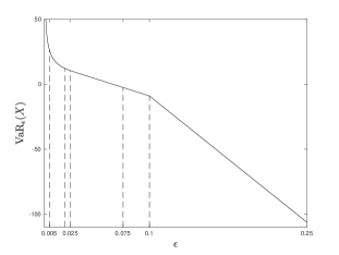
In Figure 6, we show the calibrated quantile function for the case $(\varepsilon_{1},\varepsilon_{2},\varepsilon_{3})=(0.005,0.025,0.1)$ and $(c_{1},c_{2},c_{3})=(4,3,2.5)$. Note that the condition $c_{2}\varepsilon_{2}\leqslant\varepsilon_{3}$ is needed here.

Figure 6: Calibrated quantile function when $(\varepsilon_{1},\varepsilon_{2},\varepsilon_{3})=(0.005,0.025,0.1)$ and $(c_{1},c_{2},c_{3})=(4,3,2.5)$

Although we cannot solve the $n$-point constraint problem in general, we can instead discuss calibration from a given PELVE curve, which is the problem addressed in the next section.

4 Calibration from a curve constraint

By the location-scale invariance properties of the PELVE, we know that the solution cannot be unique. Conversely, it would be interesting to ask whether all solutions can be linearly transformed from a particular solution; that is, for a given function $\varepsilon\mapsto\Pi(\varepsilon)$, whether the set $\left\{X\in\mathcal{X}:\Pi_{X}=\Pi\right\}$ is a location-scale class. This question, as well as identifying $X$ satisfying $\Pi_{X}=\Pi$, is the main objective of this section.

4.1 PELVE and dual PELVE

First, we note that calibrated distributions from an entire PELVE curve $\varepsilon\mapsto\Pi(\varepsilon)$ on $(0,1)$ would be unnatural, because the existence of the PELVE requires $\mathbb{E}[X]\leqslant\mathrm{VaR}_{\varepsilon}(X)$ which may not hold for $\varepsilon$ not very small. Thus, the PELVE curve $\Pi_{X}$ does not behave well on some parts of $(0,1)$. To address this issue, we introduce a new notion called the dual PELVE and an integral equation which can help us to calibrate the distribution by differential equations. The dual PELVE is defined by moving the multiplier in PELVE from the $\mathrm{ES}$ side to the $\mathrm{VaR}$ side.

Definition 1.

For $X\in L^{1}$, the dual PELVE function of $X$ at level $\varepsilon\in(0,1]$ is defined as

$$\pi_{X}(\varepsilon)=\inf\left\{d\geqslant 1:\mathrm{ES}_{\varepsilon}(X)\leqslant\mathrm{VaR}_{\varepsilon/d}(X)\right\},~{}~{}\varepsilon\in(0,1].$$

The existence and uniqueness of $\pi_{X}(\varepsilon)$ can be shown in the same way as the existence and uniqueness of the PELVE. There are advantages and disadvantages of working with both notions; see Li and Wang (2022, Remark 2). In our context, the main advantage of using the dual PELVE is that $\pi_{X}(\varepsilon)$ is finite for all $\varepsilon\in(0,1]$, while $\Pi_{X}(\varepsilon)$ is finite only when $\mathbb{E}[X]\leqslant\mathrm{VaR}_{\varepsilon}(X)$.

Note that for $X$ with a discontinuous quantile function, there may not exist $d$ such that $\mathrm{ES}_{\varepsilon}(X)=\mathrm{VaR}_{\varepsilon/d}(X)$. In order to guarantee the above equivalence, we make the following assumption for the quantile function, represented by general function $f$.

Assumption 1.

The function $f$ is strictly decreasing and continuous, and $\int_{0}^{1}\left|f(s)\right|\mathrm{d}s<\infty$.

Let $\mathcal{X}$ be the set of $X\in L^{1}$ with quantile function satisfying Assumption 1. The requirement that the quantile function of $X$ is continuous and strictly decreasing is equivalent to that the distribution function is continuous and strictly increasing in $(\mathrm{ess\mbox{-}inf}(X),\mathrm{ess\mbox{-}sup}(X))$; see Embrechts and Hofert (2013). We limit our discussion to random variables $X\in\mathcal{X}$, which include the most common models in risk management.

Proposition 2.

For $X$ with quantile function satisfying Assumption 1 and $\varepsilon\in(0,1)$, we have $\Pi_{X}(\varepsilon/\pi_{X}(\varepsilon))=\pi_{X}(\varepsilon)$ and $\pi_{X}(\Pi_{X}(\varepsilon)\varepsilon)=\Pi_{X}(\varepsilon)$ if $\mathbb{E}[X]\leqslant\mathrm{VaR}_{\varepsilon}(X)$. Furthermore, $\pi_{X}(\varepsilon)$ is the unique solution $d\geqslant 1$ to the equation

$$\mathrm{ES}_{\varepsilon}(X)=\mathrm{VaR}_{\varepsilon/d}(X).$$

It is straightforward to verify Proposition 2. By Proposition 2, we can calibrate the distribution functions from dual PELVE instead of PELVE, and the calibrated distributions should satisfy the equation $\mathrm{ES}_{\varepsilon}(X)=\mathrm{VaR}_{\varepsilon/d}(X)$.

4.2 An integral equation associated with dual PELVE

In order to calibrate distributions from the dual PELVE, we can equivalently focus on quantile functions. Let us consider $X\in\mathcal{X}$ and $f(s)=\mathrm{VaR}_{s}(X)$. Then, solving $\pi_{X}(\varepsilon)$ is the same as solving $z$ in following equation:

$$\int_{0}^{y}f\left(s\right)\mathrm{d}s=yf\left(zy\right)$$ (3)

for $y=\varepsilon$. The solution is $z=1/\pi_{X}(y)$. As $f(s)=\mathrm{VaR}_{s}(X)$, $f$ satisfies Assumption 1. Denote by $\mathcal{C}$ the set of all $f$ satisfying Assumption 1. For any $f\in\mathcal{C}$, the existence of the solution $z$ is guaranteed by the mean-value theorem and its uniqueness is obvious. For $y\in(0,1]$, let $z_{f}(y)$ be the solution to (3) associated with $f$. Clearly, $z_{f}(y)\leqslant 1$ and $y\mapsto yz_{f}(y)$ is strictly increasing. This is similar to Lemma 1 for the two-point case. Obviously, $z_{f}(y)$ is also location-scale invariant under linear transformation on $f\in\mathcal{C}$. That is, $z_{\lambda f+b}=z_{f}$ for $\lambda>0$ and $b\in\mathbb{R}$. Furthermore, $z_{f}$ is continuous as $f$ is continuous and strictly decreasing. The next proposition is a simple connection between $z_{f}$ and $\pi_{X}$.

Proposition 3.

For any $f$ satisfying Assumption 1, $X=f(U)$ for some $U\sim\mathrm{U}(0,1)$ has the dual PELVE $\pi_{X}(y)=1/z_{f}(y)$ for all $y\in(0,1)$ where $z_{f}$ is solution to (3). For $X$ with quantile function satisfying Assumption 1, there exists $f$ satisfying Assumption 1 such that $X=f(U)$ for some $U\sim\mathrm{U}(0,1)$ and the solution to (3) is $z_{f}(y)=1/\pi_{X}(y)$ for all $y\in(0,1)$.

Proof.

For any $f$ satisfying Assumption 1, let $F(x)=1-f^{-1}(x)$. Hence, $F$ is a continuous and strictly increasing distribution function and $F^{-1}(s)=f(1-s)$ for $s\in(0,1)$. Let $U\sim\mathrm{U}(0,1)$ and $X=F^{-1}(U)=f(1-U)$. Then $X\in\mathcal{X}$ and $X\sim F$. As $F^{-1}(1-s)=f(s)$, we have $\pi_{X}(y)=1/z_{f}(y)$. Take $U^{\prime}=1-U$. We have $X=f(U^{\prime})$ and $U^{\prime}\sim\mathrm{U}(0,1)$.

For $X\in\mathcal{X}$, let $f(s)=\mathrm{VaR}_{s}(X)$. Then, we have $z_{f}(y)=1/\pi_{X}(y)$ for $y\in(0,1]$. Furthermore, we have $F^{-1}(s)=f(1-s)$. Therefore, there exists $U\sim\mathrm{U}(0,1)$ such that $X=f(1-U)$. Let $U^{\prime}=1-U$. Then, we have $X=f(U^{\prime})$ and $U^{\prime}\sim\mathrm{U}(0,1)$. ∎

Proposition 3 allows us to study $z$ instead of $\pi$ for the calibration problem. The integral equation (3) can be very helpful in characterizing the distribution from the dual PELVE.

Some examples of $\pi_{X}$ and $z_{f}$ are listed in Table 2, which is corresponding to the PELVE presented in Table 1.

Table 2: Example of $\pi_{X}$ and $z_{f}$

$X$	$\pi_{X}(\varepsilon)$	$f$	$z_{f}$
$\mathrm{U}(0,1)$	$\pi_{X}(\varepsilon)=2$	$f(x)=1-x$	$z_{f}(y)=1/2$
$\mathrm{Exp}(\lambda)$	$\pi_{X}(\varepsilon)=e$	$f(x)=-\log(x)/\lambda$	$z_{f}(y)=1/e$
$\mathrm{GPD}(\xi)$	$\pi_{X}(\varepsilon)=(1-\xi)^{-\frac{1}{\xi}}$	$f(x)=\left\{\begin{aligned} &1/\xi\left(x^{-\xi}-1\right)&\xi\neq 0\\ &-\log(x)&\xi=0\\ \end{aligned}\right.$	$z_{f}=(1-\xi)^{\frac{1}{\xi}}$

For a given dual PELVE curve $\pi$, we find the solution to the integral equation by the following steps.

1. Let $z(y)=\frac{1}{\pi(y)}$ for all $y\in(0,1]$.

2. Find $f\in\mathcal{C}$ that satisfies $\int_{0}^{y}f(s)\mathrm{d}s=yf\left(z(y)y\right)$ for all $y\in(0,1]$.

3. By Proposition 3, $X=f(U)$ for some $U\sim\mathrm{U}(0,1)$ will have the given dual PELVE $\pi$.

Therefore, we will focus on characterizing $f$ from a given $z:(0,1]\to(0,1]$ below. Generally, it is hard to characterize $f$ explicitly. We first formulate the problem as an advanced differential equation, which helps us to find solutions.

4.3 Advanced differential equations

In this section, we show that the main objective (3) can be represented by a differential equation. The use of differential equations in computing risk measures has not been actively developed. The only paper we know is Balbás et al. (2017) which addresses a different problem.

Let us recall the integral equation (3) from Section 4.2. For a function $f\in\mathcal{C}$, we solve the function $z_{f}:(0,1)\to\mathbb{R}$ from (3). We represent (3) by an advanced differential equation using the following steps.

1. Let $\omega_{f}(y)=yz_{f}\left(y\right)$. It is easy to see that $z_{f}\left(y\right)\leqslant 1$. Hence, $\omega_{f}$ is strictly increasing and continuous on $(0,1]$ and $\omega_{f}(y)\leqslant y$.

2. Let $u_{f}$ be the inverse function of $\omega_{f}$. We have that $u_{f}:(0,z_{f}(1)]\mapsto(0,1]$ is a continuous and strictly increasing function and $u_{f}\left(w\right)\geqslant w$.

3. Replacing $y$ with $u_{f}(w)$ in (3), we have $f(w)=\int_{0}^{u_{f}(w)}f(w)\mathrm{d}s/u_{f}(w).$

4. Assume $u_{f}$ is continuously differentiable. It is clear that $f$ is continuously differentiable on $(0,z_{f}(1))$. Hence, we can represent (3) by the following advanced differential equation

   $$f^{\prime}\left(w\right)+\frac{u_{f}^{\prime}\left(w\right)}{u_{f}\left(w\right)}\left(f\left(w\right)-f\left(u_{f}\left(w\right)\right)\right)=0.$$

For a given function $z:(0,1]\to\mathbb{R}$, let $u=\omega^{-1}$ such that $\omega(y)=yz(y)$ for $y\in(0,1]$. Then, we solve the function $f$ by the following differential equation

$$f^{\prime}\left(w\right)+\frac{u^{\prime}\left(w\right)}{u\left(w\right)}f\left(w\right)-\frac{u^{\prime}\left(w\right)}{u\left(w\right)}f\left(u\left(w\right)\right)=0.$$ (4)

If $z=1/\pi_{X}$ for some $X\in\mathcal{X}$, then $u$ is a strictly increasing and continuous function such that $u\left(w\right)\geqslant w$. Furthermore, if $z$ is continuously differentiable, then we can characterize all $X\in\mathcal{X}$ with $\pi_{X}=1/z$ by (4). As $u^{\prime}\left(w\right)/u\left(w\right)\geqslant 0$ and $u(w)\geqslant w$, (4) is a linear advanced differential equation which is well studied in the literature. In Berezansky and Braverman (2011), it is shown that there exists a non-oscillatory solution for (4).

4.4 The constant PELVE curve

We first solve the case that $z(y)=c$ for all $y\in(0,1]$ and some constant $c\in\left(0,1\right)$. As we can see from Table 2, the power function and logarithm function have constant $z_{f}$. If $f(x)=\lambda x^{\alpha}+b$ for $\alpha>-1$, we can see that $(\alpha+1)^{-1/\alpha}=c$. In this section, we can characterize all the other solutions which can not be expressed as a linear transformation of the power function. That is, we will see that the set

$$\left\{f\in\mathcal{C}:z_{f}(y)=z(y),~{}y\in(0,1]\right\}$$

is not a location-scale class. Hence, we can answer the question at the beginning of the section; that is, in the case the PELVE is a constant, the set $\left\{X\in\mathcal{X}:\Pi_{X}=c\right\}$ is not a location-scale class.

Theorem 2.

For $c\in(0,1)$, any $X$ with quantile function satisfying Assumption 1 and $\pi_{X}(\varepsilon)=1/c$ for $\varepsilon\in(0,1)$ can be written as $X=f(U)$ for some $U\sim\mathrm{U}(0,1)$ and $f$ satisfying Assumption 1. Furthermore, such $f$ has the form

$$f\left(y\right)=C_{1}+C_{2}y^{\alpha}+O\left(y^{\zeta}\right),$$

where $\alpha$ is the root of $(\alpha+1)^{-1/\alpha}=c$, $\zeta>\max\{0,\alpha\}$, $C_{1},C_{2}\in\mathbb{R}$, $C_{2}\alpha<0$ and $O(y^{\zeta})$ is a function such that $\lim\sup_{y\to 0}O(y^{\zeta})/y^{\zeta}$ is a constant.

The proof of Theorem 2 is provided in Appendix B. As we can see, Theorem 2 characterizes all $X\in\mathcal{X}$ such that $\pi_{X}(\varepsilon)=1/c$. If $c\in(0,1/e)$, $\alpha$ is negative. As $\zeta>0$, we can see that $X=f(U)$ is regularly varying of index $\alpha$. Hence, one can then consider the Pareto distribution with survival function $S(x)=x^{\alpha}$ as a representative solution for the tail behavior. An open question is that, in the general case that the PELVE is not necessarily constant, whether all the solutions behave similarly regarding their tail behavior.

Another interesting implication of the theorem and its proof is that one can give a non-trivial solution for $z$ is a constant.

Example 3.

For $c\in(0,1)$, let $(\theta,\eta)$ be a solution of

$$\begin{cases}c\log c=-\frac{\eta\exp\left(-\frac{\eta}{\tan\left(\eta\right)}\right)}{\sin\left(\eta\right)},\\ \theta=-\frac{\eta}{\tan\left(\eta\right)}.\end{cases}$$

Then, the function $f$, given by

$$f(y)=C_{1}+C_{2}y^{\alpha}+C_{3}y^{\zeta}\sin(-\sigma\log(y)),\quad 0<y<1,$$ (5)

satisfies $\int_{0}^{y}f(s)\mathrm{d}s=yf(cy)$ and Assumption 1, where $\alpha$ solves $(\alpha+1)^{-1/\alpha}=c$, $\zeta=\theta/\log c-1$, $\sigma=-\eta/\log c$, $C_{2}$ is a constant such that $C_{2}\alpha<0$ and $0<C_{3}<-C_{2}\alpha/(\zeta+|\sigma|)$.

If we take $C_{3}=0$, we get the simplest power function for $z(x)=c$. If $C_{3}\neq 0$, the solution (5) is not a linear transformation of the power function solution.

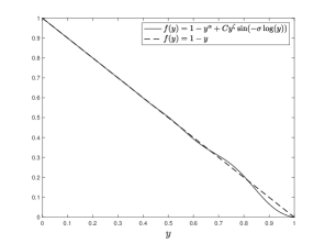
Let us look at the example where $\pi(\varepsilon)=2$ for all $\varepsilon\in(0,1]$, which means $z(y)=1/2$ for $y\in(0,1]$. As we have seen in Table 2, $f(y)=1-y$ can be a solution that leads to $X\sim\mathrm{U}(0,1)$. Furthermore, according to Example 3, we can have another solution

$$f(y)=1-y^{\alpha}+Cy^{\zeta}\sin(-\sigma\log(y)),$$

where $\alpha=1$, $C=0.05096$, $\zeta=4.0184$ and $\sigma=-15.4090$. In the left of Figure 7, we have depicted the two solutions for $f$. We can see they are quite different when $y$ goes to 1. In the right of Figure 7, we numerically calculate $z_{f}$ for $f(y)=1-y^{\alpha}+Cy^{\zeta}\sin(-\sigma\log(y))$. We can see its numerical value is almost 1/2 and the discrepancy is due to limited computational accuracy.

Figure 7: Non-unique calibrated functions for $z(y)=1/2$.

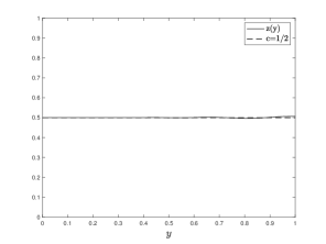
By letting $X=f(U)$, we get $\pi_{X}(\varepsilon)=2$ for all $\varepsilon\in(0,1]$ and such $X$ does not follow the uniform distribution.

4.5 A numerical method

In general, it is hard to get an explicit solution to (4). Here we present a numerical method to solve (4). Let us introduce the following process.

1. Let $a_{0}=1$, $a_{1}=a$, …,$a_{n}=u^{-1}\left(a_{n-1}\right)$.

2. For $a\in(0,1)$, let $\xi$ be the solution to $(1-\xi)^{\frac{1}{\xi}}=a$. Let

   $$f_{0}(x)=\left\{\begin{aligned} &\frac{1}{\xi}\left(x^{-\xi}-1\right),&\xi\neq 0,\\ &-\log(x),&\xi=0,\\ \end{aligned}\right.$$ (6)

   on $[a,1]$.

3. We can solve the following ODE on $\left[a_{2},a_{1}\right]$:

   $$f_{1}^{\prime}\left(w\right)+\frac{u^{\prime}\left(w\right)}{u\left(w\right)}f_{1}\left(w\right)=\frac{u^{\prime}\left(w\right)}{u\left(w\right)}f_{0}\left(u\left(w\right)\right),\quad w\in\left[a_{2},a_{1}\right].$$

4. Now we can repeat step 3 by induction on $\left[a_{n+1},a_{n}\right]$ for $n>1$ by solving

   $$f_{n}^{\prime}\left(w\right)+\frac{u^{\prime}\left(w\right)}{u\left(w\right)}f_{n}\left(w\right)=\frac{u^{\prime}\left(w\right)}{u\left(w\right)}f_{n-1}\left(u\left(w\right)\right),\quad w\in\left[a_{n+1},a_{n}\right].$$

5. In general, the solution for differential equation $\frac{dy}{dx}+P(x)y=Q(x)$ is

   $$y=e^{-\int^{x}P(\lambda)\,\mathrm{d}\lambda}\left[\int^{x}e^{\int^{\lambda}P(\varepsilon)\mathrm{d}\varepsilon}Q(\lambda)\mathrm{d}\lambda+C\right].$$

   So, we get the following solution for $f_{n}$:

   $$f_{n}\left(w\right)=e^{\int_{w}^{a_{n}}\frac{u^{\prime}(\lambda)}{u(\lambda)}\mathrm{d}\lambda}\left[f_{n-1}(a_{n})-\int_{w}^{a_{n}}e^{-\int_{\lambda}^{a_{n}}\frac{u^{\prime}(\varepsilon)}{u(\varepsilon)}\mathrm{d}\varepsilon}\frac{u^{\prime}(\lambda)}{u(\lambda)}f_{n-1}\left(u\left(\lambda\right)\right)\mathrm{d}\lambda\right],~{}w\in[a_{n+1},a_{n}].$$

6. Finally, let $f=f_{n}$ on $[a_{n+1},a_{n}]$.

Note that since we start with a strictly decreasing function, then from equation (4) we have

$$f^{\prime}(w)=\frac{u^{\prime}\left(w\right)}{u\left(w\right)}\left(f\left(u(w)\right)-f\left(w\right)\right)<0,$$

so $f$ remains strictly decreasing.

The solution produced by the numerical method heavily relies on $f_{0}$. The equation (4) does not have a unique solution, but the solution from the above process is unique. We set $f_{0}$ as (6) by assuming $z$ can be extended from $(0,1]$ to $\mathbb{R}^{+}$ and set $z(y)=a$ for all $y>1$. We use this assumption for simplification as we can know that (6) satisfies (4) for a constant $z$ from Section 4.4. This choice of $f_{0}$ is the same as the choice of $k(\varepsilon)$ in the two-point calibration problem, and this reflects our subjective view of the importance of the Pareto distribution in risk management. Especially, when $z(y)=c$ for some constant $c$, we have $u(x)=x/c$. Therefore, (5) gives

$$f_{n}(w)=\frac{a_{n}}{w}\left[f_{n-1}(a_{n})-\int_{w}^{a_{n}}\frac{1}{a_{n}}f_{n-1}\left(\frac{\lambda}{c}\right)\mathrm{d}\lambda\right].$$

If we set $f_{0}$ as (6), we can have $f_{1}$ also in the form of (6). Then, it is obvious that $f_{n}$ is also in the form of (6). Therefore, the numerical method gives the simplest power function or logarithm function when $z(y)$ is a constant on $(0,1]$ as Table 2, which leads to the generalized Pareto distribution for $X$.

4.6 Numerical calibrated quantile function

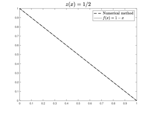
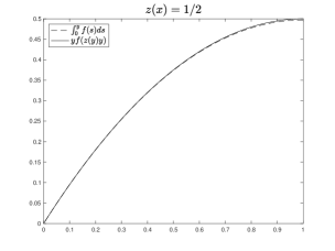
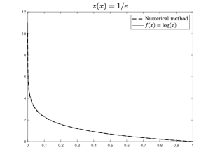
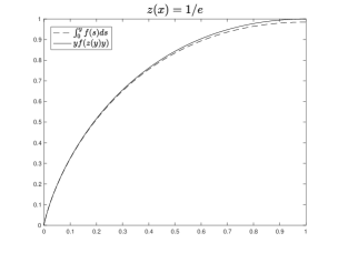
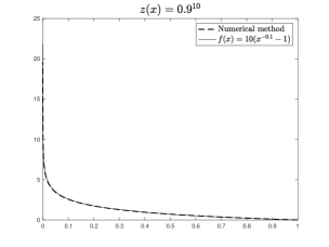
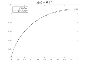
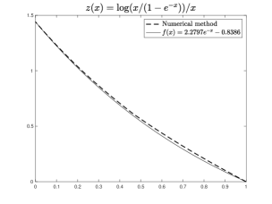
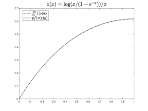
Now let us explore the method in Section 4.5 with simulation. Here we present the results for a few cases. In Figures 8 to 11, we compare the solution from the numerical method with the standard formula in Table 2 in the left panel, and compare $\int_{0}^{y}f(s)\mathrm{d}s$ with $yf(z(y)y)$ to validate the equation (3) in the right panel.

We first try some examples where $z$ is constant as shown in Table 2, i.e. $z(x)=1/2$ (Figure 8), $z(x)=1/e$ (Figure 9) and $z(x)=0.9^{10}$ (Figure 10). For Figure 8 to 10, we can see that the numerical method provides exactly the same function $f$ as Table 2.

In Figure 11, we check the case $z(x)=\log\left(x/(1-e^{-x})\right)/x$. The function $f(x)=e^{-x}$ satisfies (3). We can see that the solution from the numerical method is close to a function of the form $f(x)=\lambda e^{-x}+b$, which is known to satisfy the integral equation.

Figure 8: Calibrated function and validation for $z(x)=1/2$

Figure 9: Calibrated function and validation for $z(x)=1/e$

Figure 10: Calibrated function and validation for $z(x)=0.9^{10}$

Figure 11: Calibrated function and validation for $z(x)=\log\left(x/(1-e^{-x})\right)/x$

5 Technical properties of the PELVE

We now take a turn to study several additional properties of PELVE. In particular, we will obtain results on the monotonicity and convergence of the dual PELVE as well as the PELVE.

5.1 Basic properties of dual PELVE

The following proposition that shows the PELVE and dual PELVE share some basic properties such as monotonicity (i), location-scale invariance (ii) and shape relevance (iii)-(iv) below.

Proposition 4.

Suppose the quantile function of $X$ satisfies Assumption 1 and $\varepsilon\in(0,1]$.

1. $\Pi_{X}(\varepsilon)$ is increasing (decreasing) in $\varepsilon$ if and only if so is $\pi_{X}(\varepsilon)$.

2. For all $\lambda>0$ and $a\in\mathbb{R}$, $\pi_{\lambda X+a}(\varepsilon)=\pi_{X}(\varepsilon)$.

3. $\pi_{f(X)}(\varepsilon)\leqslant\pi_{X}(\varepsilon)$ for all strictly increasing concave functions: $f:\mathbb{R}\to\mathbb{R}$ with $f(X)\in\mathcal{X}$.

4. $\pi_{g(X)}(\varepsilon)\geqslant\pi_{X}(\varepsilon)$ for all strictly increasing convex functions: $g:\mathbb{R}\to\mathbb{R}$ with $g(X)\in\mathcal{X}$.

The statements (ii)-(iv) are parallel to the corresponding statements in Theorem 1 of Li and Wang (2022) on PELVE. The proof of Proposition 4 is put in Appendix C. Proposition 4 allows us to study the monotonicity and convergence of the PELVE by analyzing the corresponding properties of the dual PELVE, which is more convenient in many cases. In the following sections, we focus on finding the conditions which make the dual PELVE monotone and convergent at 0. By Proposition 4, those conditions can also apply to the PELVE.

5.2 Non-monotone and non-convergent examples

In this section, we study the monotonicity and convergence of dual PELVE. For monotonicity, we have shown some well-known distributions such as normal distribution, t-distribution and lognormal distribution have monotone PELVE curves in Example 3. However, the PELVE is not monotone for all $X\in\mathcal{X}$. Below we provide an example.

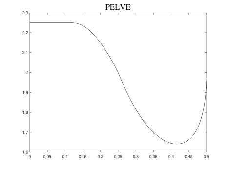
Example 4 (Non-monotone PELVE).

Let us consider the following density function $g$ on $[-2,2]$,

$$g\left(x\right)=\frac{1}{2}\left((x+2)\mathds{1}_{\{x\in[-2,-1]\}}-x\mathds{1}_{\{x\in(-1,0]\}}+x\mathds{1}_{\{x\in(0,1]\}}+(2-x)\mathds{1}_{\{x\in(1,2]\}}\right).$$

For $X$ with density function $g$, Figure 12 presents the value of $\Pi_{X}(\varepsilon)$ for $\varepsilon\in(0,0.5)$. As one can see, the PELVE is not necessarily decreasing, and so is the dual PELVE.

Figure 12: PELVE for $X$ with density $g$

For the convergence, it is clear that $\pi_{X}(\varepsilon)$ is continuous in $(0,1)$ for $X\in\mathcal{X}$. Therefore, $\lim_{\varepsilon\to p}\pi_{X}(\varepsilon)$ exists for all $p\in(0,1)$. However, both $\Pi_{X}(\varepsilon)$ and $\pi_{X}(\varepsilon)$ are not well defined at $\varepsilon=0$. If $\lim_{\varepsilon\to 0}\pi_{X}(\varepsilon)$ exists, we can define $\pi_{X}(0)$ as the limit, and $\Pi_{X}(0)$ similarly. However, the following example shows that the limit does not exist for some $X\in\mathcal{X}$.

Example 5 (No limit at 0).

We can construct a random variable $X\in\mathcal{X}$ such that $\lim_{\varepsilon\to 0}\pi_{X}(\varepsilon)$ does not exist from the integral equation (3) in Section 4.2. Equivalently, we will find a continuous and strictly decreasing function $f\in\mathcal{C}$ such that $\lim_{y\to 0}z_{f}(y)$ does not exist. Let $c$ be the Cantor ternary function on $[0,1]$. Note that $x\mapsto c(x)$ is continuous and increasing on $(0,1)$ and $c(x/3)=c(x)/2$. Let $f(x)=-c(x)-x^{\log 2/\log 3}$. It is clear that $f\in\mathcal{C}$ and $f(x/3)=f(x)/2$. For each $y\in(0,1]$, we have

$$yf\left(z_{f}(y)y\right) =\int_{0}^{y}f(x)\mathrm{d}x$$

$$=2\int_{0}^{y}f\left(\frac{1}{3}x\right)\mathrm{d}x=6\int_{0}^{\frac{1}{3}y}f(x)\mathrm{d}x=2yf\left(\frac{1}{3}yz_{f}\left(\frac{1}{3}y\right)\right)=yf\left(yz_{f}\left(\frac{1}{3}y\right)\right).$$

Since $f$ is strictly decreasing, $z_{f}(y)=z_{f}(y/3)$ for $y\in(0,1]$. It means that $z_{f}(y)$ is a constant on $(0,1]$ if $\lim_{y\to 0}z_{f}(y)$ exists. Now, let us look at two particular points of $z_{f}(y)$. We can show that $z_{f}(1)\neq z_{f}(4/9)$. Let $z=(\log 2/\log 3+1)^{-(\log 3/\log 2)}$. Then, we have $1/3<z\approx 0.46<1/2$. For $y=1$, we have $\int_{0}^{1}c(s)\mathrm{d}s=c(z)=1/2$ and $\int_{0}^{c}s^{\log 2/\log 3}\mathrm{d}s=z^{\log 2/\log 3}$. Therefore, we get $z_{f}(1)=z<1/2$. For $y=4/9$, we have

$$f\left(\frac{4}{9}z_{f}\left(\frac{4}{9}\right)\right) =\frac{9}{4}\int_{0}^{4/9}f(s)\mathrm{d}s$$

$$=-\frac{9}{4}\left(\frac{1}{\frac{\log 2}{\log 3}+1}\left(\frac{4}{9}\right)^{\frac{\log 2}{\log 3}+1}+\frac{1}{12}+\frac{1}{2}\left({\frac{4}{9}-\frac{1}{3}}\right)\right)<-0.68<f\left(\frac{2}{9}\right)\approx-0.64.$$

As $f$ is strictly decreasing, we have $(4/9)z_{f}(4/9)>2/9$ which implies $z_{f}(4/9)>1/2>z_{f}(1)$. As a result, $\lim_{y\to 0}z_{f}(y)$ does not exist. Therefore, we have a continuous and strictly decreasing $f$ such that $\lim_{y\to 0}z_{f}(y)$ does not exist.

5.3 Sufficient condition for monotonicity and convergence

In risk management applications, for a random variable $X$ modeling a random loss, the behavior of its tail is the most important. Let $F^{[p,1]}$ be the upper $p$-tail distribution of $F$ (see e.g., Liu and Wang (2021)), namely

$$F^{[p,1]}(x)=\frac{(F(x)-p)_{+}}{1-p},~{}~{}~{}x\in\mathbb{R}.$$

We will see that the dual PELVE of $F^{[p,1]}$ is a part of the dual PELVE of $F$.

Lemma 2.

Let $F$ be the distribution function of $X$ with quantile function satisfying Assumption 1. For $p\in(0,1)$ and $X^{\prime}\sim F^{[p,1]}$, it holds

$$\pi_{X^{\prime}}(\varepsilon)=\pi_{X}(\varepsilon(1-p)).$$

Proof.

It is clear that $\mathrm{VaR}_{\varepsilon}(X^{\prime})=\mathrm{VaR}_{{\varepsilon(1-p)}}(X)$ and $\mathrm{ES}_{\varepsilon}(X^{\prime})=\mathrm{ES}_{{\varepsilon(1-p)}}(X)$. Therefore,

$$\pi_{X^{\prime}}(\varepsilon) =\inf\{d\geqslant 1:\mathrm{ES}_{\varepsilon}(X^{\prime})\leqslant\mathrm{VaR}_{\varepsilon/d}(X^{\prime})\}$$

$$=\inf\{d\geqslant 1:\mathrm{ES}_{\varepsilon(1-p)}(X^{\prime})\leqslant\mathrm{VaR}_{\varepsilon(1-p)/d}(X^{\prime})\}=\pi_{X}(\varepsilon(1-p)).$$

Thus, we have the desired result. ∎

The tail distribution can provide a condition to check whether the dual PELVE is decreasing.

Proposition 5.

Let $F$ be the distribution function of $X$ with quantile function satisfying Assumption 1. If $x\mapsto F^{-1}\big{(}(1-p)F(x)+p\big{)}$ is convex (concave) for all $p\in(0,1)$, then $\pi_{X}$ and $\Pi_{X}$ are decreasing (increasing).

Proof.

For any $p\in(0,1)$, let $X^{\prime}\sim F^{[p,1]}$. By Lemma 2, we have $\pi_{X^{\prime}}(\varepsilon)=\pi_{X}(\varepsilon(1-p))$. Furthermore, we have

$${\left(F^{[p,1]}\right)}^{-1}(t) =F^{-1}\left((1-p)t+p\right)=F^{-1}\Big{(}(1-p)F\big{(}F^{-1}(t)\big{)}+p\Big{)},\quad t\in[0,1].$$

Let $U\sim\mathrm{U}(0,1)$, $X=F^{-1}(U)$ and $X^{\prime}=(F^{[p,1]})^{-1}(U)$.

We assume that $x\mapsto F^{-1}\big{(}(1-p)F(x)+p\big{)}$ is a convex function on $(\mathrm{ess\mbox{-}inf}(X),\mathrm{ess\mbox{-}sup}(X))$ first. Let $f:\mathbb{R}\to\mathbb{R}$ be a strictly increasing convex function such that $f(x)=F^{-1}((1-p)F(x)+p)$ for $x\in(\mathrm{ess\mbox{-}inf}(X),\mathrm{ess\mbox{-}sup}(X)).$ Then, we have $X^{\prime}=f(X)$. By Proposition 4, we get $\pi_{X^{\prime}}(\varepsilon)\geqslant\pi_{X}(\varepsilon)$. As $\pi_{X^{\prime}}(\varepsilon)=\pi_{X}(\varepsilon(1-p))$, we have $\pi_{X}(\varepsilon(1-p))\geqslant\pi_{X}(\varepsilon)$ for all $p\in(0,1)$. Thus, $\pi_{X}$ is decreasing. By Proposition 4, we have $\Pi_{X}$ is also decreasing.

On the other hand, if $x\mapsto F^{-1}\big{(}(1-p)F(x)+p\big{)}$ is concave, we have $\pi_{X}(\varepsilon(1-p))\leqslant\pi_{X}(\varepsilon)$ for all $p\in(0,1)$ and $\pi_{X}$ is increasing. So is $\Pi_{X}$. ∎

The condition $x\mapsto F^{-1}\big{(}(1-p)F(x)+p\big{)}$ is convex (concave) for all $p\in(0,1)$ is generally hard to check. Intuitively, this condition means that $F^{[p,1]}$ has a less heavy tail compared to $F$. We can further simplify this condition by using the hazard rate function. For $X\in\mathcal{X}$ with distribution function $F$ and density function $f$, let $S=1-F$ be the survival function and $\eta=f/S$ be the hazard rate function. As $F$ is continuous and strictly increasing, $S$ is continuous and strictly decreasing.

Theorem 3.

For $X$ with quantile function satisfying Assumption 1, let $\eta$ be the hazard rate function of $X$. If $1/\eta$ is second-order differentiable and convex (concave), then $\pi_{X}$ and $\Pi_{X}$ are decreasing (increasing).

The proof of Theorem 3 is provided in Appendix C.

Example 6.

For the normal distribution, we can give a short proof of the convexity of $1/\eta$. Let $S$ be the survival function of the standard normal distribution and $f$ its density. Let $I\left(x\right)=1/\eta\left(x\right)=S(x)/f(x)=\exp\left(x^{2}/2\right)\int_{-\infty}^{-x}\exp\left(-s^{2}/2\right)\mathrm{d}s$. One can easily see that

$$I^{\prime}\left(x\right)=xI\left(x\right)-1$$ (7)

which gives $I^{\prime\prime}\left(x\right)=xI^{\prime}\left(x\right)+I\left(x\right)$. This with (7) implies that

$$I^{\prime\prime}\left(x\right)=\left(1+x^{2}\right)I\left(x\right)-x.$$ (8)

First, consider the negative line i.e., $x<0$. In this case (7) and (8) imply $I^{\prime}(x)=xI(x)-1<0,$ and $I^{\prime\prime}(x)=(1+x^{2})I(x)+(-x)>0.$ The implication of the two relations is that $I$ is a convex and decreasing function on negative line. Now we consider the case $x>0$. In this case, let $i\left(x\right)=I^{\prime}\left(-x\right)$. From what we have proved it is clear that $i$ is an increasing function on $x>0$. On the other hand, we have $I\left(x\right)+I\left(-x\right)=1/f\left(x\right)=\sqrt{2\pi}\exp\left(x^{2}/2\right)$. This combined with (7) gives us

$$I^{\prime}\left(x\right)=x\left(I\left(x\right)+I\left(-x\right)\right)+i\left(x\right)=x\sqrt{2\pi}\exp\left(x^{2}/2\right)+i\left(x\right),x>0.$$

This means $I^{\prime}$ is an increasing function on $x>0$ as it is a summation of two other increasing functions, so $I$ is convex on the positive line as well.

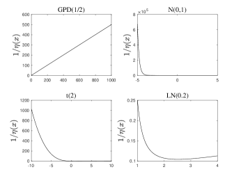
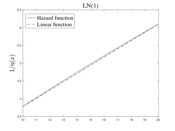
Figure 13 presents the curve $1/\eta$ for the generalized Pareto distribution, the Normal distribution, the t-distribution and the Lognormal distribution. For distributions $\mathrm{GPD}(1/2)$, $\mathrm{N}(0,1)$ and $\mathrm{t}(2)$, we can see that the curves $1/\eta$ are convex, and this coincides with decreasing PELVE shown in Example 2. For the Lognormal distribution, the shape of $1/\eta$ depends on $\sigma$. As shown in Example 2, the PELVE for $\mathrm{LN}(\sigma)$ is visibly decreasing for $\sigma^{2}=0.04$ and increasing for $\sigma=1$. Corresponding to the above observations, we see that $1/\eta$ is convex for $\sigma^{2}=0.04$ and concave for $\sigma^{2}=1$.

Figure 13: $1/\eta$ for $\mathrm{GPD}(1/2)$, $\mathrm{N}(0,1)$, $\mathrm{t}(2)$, $\mathrm{LN}(0,2)$ and $\mathrm{LN}(1)$ in blue curves; in the right panel, the red curve is linear

Corollary 1.

If the hazard rate of a random variable $X$ is second-order differentiable and concave, then $\pi_{X}$ and $\Pi_{X}$ are decreasing.

Proof.

Just note that if $\eta$ is concave, then $\eta\eta^{\prime\prime}$ is non-positive. It follows that

$$\left(\frac{1}{\eta}\right)^{\prime\prime}=\left(-\frac{\eta^{\prime}}{\eta^{2}}\right)^{\prime}=\frac{2\left(\eta^{\prime}\right)^{2}-{{\eta\eta^{\prime\prime}}}}{\eta^{3}}\geqslant 0.$$

Thus, ${1}/{\eta}$ is convex, and the desired statement follows from Theorem 3. ∎

The corollary above is a result of the fact that the concavity of $\eta$ implies convexity of $1/\eta$. Therefore, concave $\eta$ always leads to decreasing PELVE. For example, the Gamma distribution $\mathrm{G}(\alpha,\lambda)$ with density $f(x)=\lambda^{\alpha}t^{\alpha-1}e^{-\lambda t}/\Gamma(\alpha)$ has concave hazard rate function when $\alpha>1$. Furthermore, by Theorem 3, we can easily find more well-known distributions that have decreasing $\pi_{X}$.

As the tail distribution determines $\pi_{X}$ around $0$, we can focus on the tail distribution to discuss the convergence of $\pi_{X}$ at $0$. Note that if the survival distribution function is regularly varying, then its tail parameter one-to-one corresponds to the limit of $\Pi_{X}$ at $0$ as shown by Theorem 3 of Li and Wang (2022). Hence, the limit of $\Pi_{X}$, if it exists, can be useful as a measure of tail heaviness, and it is well defined even for distributions that do not have a heavy tail. By the monotone convergence theorem, we have $\lim_{\varepsilon\to 0}\pi_{X}(\varepsilon)$ exists if $\pi_{X}$ is monotone. The limit may be finite or infinite.

Corollary 2.

For $X$ with quantile function satisfying Assumption 1, let $\eta$ be the hazard rate of $X$. If $1/\eta(x)$ is second-order differentiable and convex (concave) in $\left(F^{-1}(\delta),\mathrm{ess\mbox{-}sup}(X)\right)$ for some $\delta\in(0,1)$, then $\lim_{\varepsilon\to 0}\pi_{X}(\varepsilon)$ exists. In particular, this is true if $\eta$ is second-order differentiable and concave on $\left(F^{-1}(\delta),\mathrm{ess\mbox{-}sup}(X)\right)$.

Proof.

Let $X^{\prime}\sim F^{[\delta,1]}$. Then, the survival function for $X^{\prime}$ is $S_{X^{\prime}}(x)=S(x)/(1-p)$ for $x\geqslant F^{-1}(\delta)$. The density function is $f_{X^{\prime}}(x)=f(x)/(1-p)$ for $x\geqslant F^{-1}(\delta)$. Therefore, the hazard rate function is $\eta_{X^{\prime}}(x)=f(x)/S(x)=\eta(x)$ for $x\geqslant F^{-1}(\delta)$.

As $1/\eta(x)$ is convex (concave) when $x>F^{-1}(\delta)$, we have $1/\eta_{X^{\prime}}(x)$ is convex (concave). By Theorem 3, we have $\pi_{X^{\prime}}(\varepsilon)$ is decreasing (increasing) on $(0,1)$. As a result, we have $\pi_{X}(\varepsilon)$ is decreasing (increasing) on $(0,\delta)$ and $\lim_{\varepsilon\to 0}\pi_{X}(\varepsilon)$ exists.

By Corollary 1, if $\eta$ is concave on $(F^{-1}(\delta),\mathrm{ess\mbox{-}sup}(X))$, $1/\eta$ is convex on $(F^{-1}(\delta),\mathrm{ess\mbox{-}sup}(X))$ and $\lim_{\varepsilon\to 0}\pi_{X}(\varepsilon)$ also exists. ∎

Example 7.

If $\lim_{\varepsilon\to 0}\pi_{X}(\varepsilon)$ is a constant, we have $\lim_{\varepsilon\to 0}\Pi_{\varepsilon}(X)=\lim_{\varepsilon\to 0}\pi_{X}(\varepsilon)$ as $\pi_{X}(\Pi_{X}(\varepsilon)\varepsilon)=\Pi_{X}(\varepsilon)$. We give the numerical values of $\Pi_{X}(\varepsilon)$ at very small probability levels $\varepsilon$ for normal, t, and log-normal distributions. These distributions do not have a constant PELVE curve, and using Corollary 2 we can check that their PELVE have limits. As we can see from Table 3, PELVE can still distinguish the heaviness of the tail even when $\varepsilon$ is very small. The heavier tailed distributions report a higher PELVE value. For the normal distribution and the log-normal distribution with $\sigma=0.2$, the value of PELVE is close to $e\approx 2.7183$ as $\varepsilon\downarrow 0$. From the numerical values, it is unclear whether $\Pi_{X}(\varepsilon)\to e$ for all log-normal distributions, but there is no practical relevance to compute $\Pi_{X}(\varepsilon)$ for $\varepsilon<10^{-11}$ in applications.

Table 3: Values of $\Pi_{X}(\varepsilon)$

Distribution	N	LN($1$)	LN($0.5$)	LN($0.2$)	t($2$)	t($3$)
$\varepsilon={10}^{-10}$	2.6884	2.9167	2.7944	2.7290	4.0000	3.3750
$\varepsilon={10}^{-11}$	2.6909	2.9077	2.7920	2.7287	4.0000	3.3750

6 Applications to datasets used in insurance

In this section, we apply the PEVLE calibration techniques to datasets used in insurance to show how to use the calibrated distribution in estimating risk measure values and simulation.

6.1 Dental expenditure data

In this example, we apply the calibration model to the 6494 complete household component’s total dental expenditure data from Medical Expenditure Panel Survey for 2020. An earlier version of the same dataset is used by Behan et al. (2010) to study the relationship between worker absenteeism and overweight or obesity. The main purpose of this experiment is to construct tractable models, with continuous and simple quantile functions, which have similar risk measure values as the original dataset, and the same PELVE at certain levels. We present in Figure 14 two quantile functions calibrated from $\Pi_{X}(\varepsilon_{1})$ and $\Pi_{X}(\varepsilon_{2})$, with $(\varepsilon_{1},\varepsilon_{2})=(0.01,0.05)$ and $(\varepsilon_{1},\varepsilon_{2})=(0.05,0.1)$, respectively. The two calibrated quantile functions are scaled up according to the empirical $\mathrm{VaR}_{\varepsilon_{1}}(X)$ and $\mathrm{VaR}_{\varepsilon_{2}}(X)$. By Theorem 1, we can calibrate the quantile functions from Case 4 when $(\varepsilon_{1},\varepsilon_{2})=(0.01,0.05)$, and from Case 5 when $(\varepsilon_{1},\varepsilon_{2})=(0.05,0.1)$. As mentioned before, for $(\varepsilon_{1},\varepsilon_{2})=(0.05,0.1)$, we set the calibrated quantile function in $(0,c_{1}\varepsilon_{1})$ as the Pareto quantile function. Hence, there is no flat part in the two calibrated quantile functions shown in Figure 14. As we can see, both the two calibrated quantile functions fit the empirical quantile functions well. The calibrated quantile function can be regarded as a special parameterized model for tail distribution, which can fit the value of $\mathrm{VaR}$ and $\mathrm{ES}$ at specified levels. With the parameterized calibrated model, we can estimate the value of tail risk measures (see Liu and Wang (2021)) such as ES, VaR, and Range-VaR (RVaR), amongst others. In Tables 4 and 5, we compute the values of ES and RVaR for the calibrated model and compare them with empirical ES and RVaR values, respectively, where the risk measure RVaR is defined as

$$\mathrm{RVaR}_{\alpha,\beta}(X)=\frac{1}{\beta-\alpha}\int_{\beta}^{\alpha}\mathrm{VaR}_{\gamma}(X)\mathrm{d}\gamma$$

for $0\leqslant\alpha<\beta<1$; see Cont et al. (2010) and Embrechts et al. (2018). As we scale the calibrated quantile function to empirical $\mathrm{VaR}_{\varepsilon_{1}}(X)$ and $\mathrm{VaR}_{\varepsilon_{2}}(X)$, the calibrated ES and empirical ES are identical at levels $\varepsilon_{1}\Pi_{X}(\varepsilon_{1})$ and $\varepsilon_{2}\Pi_{X}(\varepsilon_{2})$ by the definition of PELVE. For other probability levels, the calibrated ES and RVaR in Tables 4 and 5 are close to their empirical counterparts. When $(\varepsilon_{1},\varepsilon_{2})=(0.01,0.05)$, it may only be useful to compute calibrated $\mathrm{ES}_{p}(X)$ for $p<0.05\Pi_{X}(0.05)=0.11591$ because the calibrated quantile function is arbitrary beyond the level $0.11591$. If we need to estimate ES or RVaR for a larger probability level, we can choose a higher $\varepsilon_{2}$ as long as $\mathbb{E}[X]\leqslant\mathrm{VaR}_{\varepsilon_{2}}(X)$ is satisfied. For this dataset, the highest $\varepsilon_{2}$ we can use is 0.1983.

Using the methods in Section 3, for quantile levels between $(0,\varepsilon_{1})$, the distribution calibrated from one point $(\varepsilon_{1},c_{1})$ is the same as the one calibrated from two points $(\varepsilon_{1},c_{1})$ and $(\varepsilon_{2},c_{2})$. Hence, the results for $\mathrm{ES}_{p}$ of the one-point calibrated function are also shown in Tables 4 and 5 in the cells $p\leqslant\varepsilon_{1}$.

Figure 14: Empirical and calibrated $\mathrm{VaR}_{\varepsilon}$ for the dental expenditure data

Table 4: Empirical ES and calibrated ES for the dental expenditure data

$p$	0.01	0.05	0.1	0.2	0.3
Empirical $\mathrm{ES}_{p}$	10073.1	5361.7	3624.8	2317.9	1696.7
Calibrated $\mathrm{ES}_{p}$ from $(\varepsilon_{1},\varepsilon_{2})=(0.01,0.05)$	11703.9	5357.7	3759.1	-	-
Calibrated $\mathrm{ES}_{p}$ from $(\varepsilon_{1},\varepsilon_{2})=(0.05,0.1)$	10878.1	5439.6	3711.3	2293.7	1696.4

Table 5: Empirical RVaR and calibrated RVaR for the dental expenditure data

$(\alpha,\beta)$	$(0.01,0.02)$	$(0.02,0.05)$	$(0.05,0.1)$
Empirical $\mathrm{RVaR}_{\alpha,\beta}$	5748.5	3662.4	1887.9
Calibrated $\mathrm{RVaR}_{\alpha,\beta}$ from $(\varepsilon_{1},\varepsilon_{2})=(0.01,0.05)$	5003.7	3360.2	2160.6
Calibrated $\mathrm{RVaR}_{\alpha,\beta}$ from $(\varepsilon_{1},\varepsilon_{2})=(0.05,0.1)$	5634.6	3561.8	1983.1

6.2 Hospital costs data

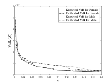
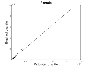
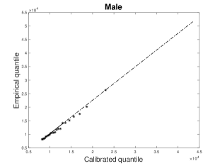
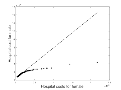
In this example, we apply the calibration process to the Hospital Costs data of Frees (2009) which were originally from the Nationwide Inpatient Sample of the Healthcare Cost and Utilization Project (NIS-HCUP). The data contains 500 hospital costs observations with 244 males and 256 females which can be regarded as the losses of the health insurance policies. Using the calibration model of the two-point constraint problem, we calibrate quantile functions for females and males from PELVE at probability levels $\varepsilon_{1}=0.05$ and $\varepsilon_{2}=0.1$, which are shown in Figure 15. Except for estimating the risk measure, the calibrated distribution is useful in simulation. Assume the insurance company wants to know the top 10% hospital costs; that is $X|X>\mathrm{VaR}_{0.1}(X)$ where $X$ is the hospital costs. There are only 24 available data for males and 25 available data for females, which would be not enough for making statistically solid decisions. To generate more pseudo-data points, we can simulate data from the calibrated distribution; that is, we simulate data from $F^{[p,1]}$ where $F$ is the calibrated distribution in Figure 15. Taking $p=0.9$, we have $F^{[p,1]}(t)=\mathrm{VaR}_{(1-p)(1-t)}(X)$ with $\mathrm{VaR}_{t}(X)$ from Figure 15. We simulate 1000 data from the calibrated distributions based on PELVE at $\varepsilon_{1}=0.05$ and $\varepsilon_{2}=0.1$. In Figure 16, we present two QQ plots of simulated data against empirical data for females and males respectively. As we can see, the simulated data has a similar distribution as the empirical data. Those simulated pseudo-data points can be used for estimating risk measures or making other decisions. For example, the simulated hospital cost can be used to design health insurance contrasts or set the premium in complex systems, where sometimes methods based on simulated data are more convenient to work with than methods relying on distribution functions. This may be seen as an alternative, smoothed, version of bootstrap; recall that the classic bootstrap sample can only take the values represented in the dataset. Furthermore, we compare the simulated data of hospital costs for females and males in Figure 17, which shows that the distribution of the hospital costs for females has a heavier tail than that for males.

Figure 15: Empirical and calibrated $\mathrm{VaR}_{\varepsilon}$ for the hospital costs data

(a) Hospital costs for female

(b) Hospital costs for male

Figure 16: QQ plot: simulated data VS empirical data

Figure 17: QQ plot of simulated data of hospital costs: female VS male

7 Conclusion

In this paper, we offer several contributions to the calibration problem and properties of the PELVE. The calibration problem concerns, with some given values from a PELVE curve, how one can build a distribution that has this PELVE. We solve a few settings of calibration based on a one-point constraint, a two-point constraint, or the entire curve constraint. In particular, the calibration for a given PELVE curve involves solving an integral equation $\int_{0}^{y}f\left(s\right)\mathrm{d}s=yf\left(z\left(y\right)y\right)$ for a given function $z$, and this requires some advanced analysis and a numerical method in differential equations. For the case that $z$ is a constant curve, we can identify all solutions, which are surprisingly complicated. In addition, we see that if $\pi_{X}$ is a constant larger than $e$, which is observed from typical values in financial return data (Li and Wang (2022)), $X$ share the same tail behavior with the corresponding Pareto solution. We also applied our calibration techniques to two datasets used in insurance.

On the technical side, we study whether the PELVE is monotone and whether it converges at 0. We show that the monotonicity of the PELVE is associated with the shape of the hazard rate. If the inverse of the hazard rate is convex (concave), the PELVE is decreasing (increasing). The monotonicity at the tail part of the PELVE leads to conditions to check the convergence of the PELVE at $0$. If the inverse of the hazard rate is convex (concave) at the tail of the distribution, the limit of the PELVE at $0$ exists.

There are several open questions related to PELVE that we still do not fully understand. One particular such question is whether the tail behavior, e.g., tail index, of a distribution is completely determined by its PELVE. We have seen that this holds true in the case of a constant PELVE (see Theorem 2), but we do not have a general conclusion. In the case of regularly varying survival functions, Li and Wang (2022, Theorem 3) showed that the limit of PELVE determines its tail parameter, but it is unclear whether this can be generalized to other distributions. Another challenging task is, for a specified curve $\pi$ on $[0,1]$, to determine whether there exists a model $X$ with $\pi_{X}=\pi$. The case of $n$-point constraints for large $n$ may require a new design of verification algorithms. This question concerns the compatibility of given information with statistical models, which has been studied, in other applications of risk management, by Embrechts et al. (2002, 2016) and Krause et al. (2018).

Acknowledgements

The authors thank Xiyue Han for many helpful comments. Ruodu Wang is supported by the Natural Sciences and Engineering Research Council of Canada (RGPIN-2018-03823, RGPAS-2018-522590).

Appendix A Omitted proofs in Section 3

Proof of Lemma 1.

As $\mathbb{E}[X]\leqslant\mathrm{VaR}_{\varepsilon_{2}}(X)$ and $\varepsilon_{1}<\varepsilon_{2}$, $\mathbb{E}[X]\leqslant\mathrm{VaR}_{\varepsilon_{2}}(X)\leqslant\mathrm{VaR}_{\varepsilon_{1}}(X)$. By Proposition 1 in Li and Wang (2022), $\Pi_{X}(\varepsilon_{1})<\infty$ and $\Pi_{X}(\varepsilon_{2})<\infty$.

For any $\varepsilon\in(0,1)$ satisfying $\mathbb{E}[X]\leqslant\mathrm{VaR}_{\varepsilon}(X)$,

$$\varepsilon\Pi_{X}(\varepsilon) =\varepsilon\inf\{c\in[1,1/\varepsilon]:\mathrm{ES}_{c\varepsilon}(X)\leqslant\mathrm{VaR}_{\varepsilon}(X)\}$$

$$=\inf\{\varepsilon c\in[\varepsilon,1]:\mathrm{ES}_{c\varepsilon}(X)\leqslant\mathrm{VaR}_{\varepsilon}(X)\}$$

$$=\inf\{k\in[\varepsilon,1]:\mathrm{ES}_{k}(X)\leqslant\mathrm{VaR}_{\varepsilon}(X)\}.$$

Let $A(\varepsilon)=\{k\in[\varepsilon,1]:\mathrm{ES}_{k}(X)\leqslant\mathrm{VaR}_{\varepsilon}(X)\}$. For any $k\in A(\varepsilon_{2})$, we have $1\geqslant k\geqslant\varepsilon_{2}>\varepsilon_{1}$ and $\mathrm{ES}_{k}(X)\leqslant\mathrm{VaR}_{\varepsilon_{2}}(X)\leqslant\mathrm{VaR}_{\varepsilon_{1}}(X)$. Hence, $k\in A(\varepsilon_{1})$ and this gives $A(\varepsilon_{2})\subseteq A(\varepsilon_{1})$. Therefore, $\varepsilon_{2}\Pi_{X}(\varepsilon_{2})=\inf A(\varepsilon_{2})\geqslant\inf A(\varepsilon_{1})=\varepsilon_{1}\Pi_{X}(\varepsilon_{1})$. ∎

Proof of Theorem 1.

We will check the equivalent condition (2) between $\mathrm{VaR}$ and $\mathrm{ES}$. Note that if $t\mapsto\mathrm{VaR}_{t}(X)$ is a constant on $(0,\varepsilon)$, then $\Pi_{X}(\varepsilon)=1$. If $t\mapsto\mathrm{VaR}_{t}(X)$ is not a constant on $(0,\varepsilon)$, then $\Pi_{X}(\varepsilon)$ is the unique solution that satisfies $\mathrm{ES}_{\varepsilon\Pi_{X}(\varepsilon)}(X)=\mathrm{VaR}_{\varepsilon}(X)$.

1. Case 1, $c_{2}=1$. It is clear that $\mathrm{VaR}_{t}(X)$ is a constant for $t\in(0,c_{2}\varepsilon_{2}]$ and (2) is satisfied. Hence, $\Pi_{X}(\varepsilon_{2})=1.$ Moreover, $\mathrm{VaR}_{t}(X)$ is also a constant for $t\in(0,c_{1}\varepsilon_{1}]$, which implies $\Pi_{X}(\varepsilon_{1})=1$.

2. Case 2, $c_{1}=1$ and $1<c_{2}\leqslant 1/\varepsilon_{2}$. For $t\in(0,\varepsilon_{1})$, $\mathrm{VaR}_{t}(X)=G_{\mathbf{z}}(t)$ is a constant for $t\in(0,c_{1}\varepsilon_{1})$. Hence, $\Pi_{X}(\varepsilon_{1})=1$. Next, we check whether $\mathrm{ES}_{c_{2}\varepsilon_{2}}(X)=\mathrm{VaR}_{\varepsilon_{2}}(X)$. The value of $\mathrm{ES}_{c_{2}\varepsilon_{2}}(X)$ is

   $$\mathrm{ES}_{c_{2}\varepsilon_{2}}(X)$$

   $$=\frac{1}{c_{2}\varepsilon_{2}}\left(\int_{0}^{\varepsilon_{1}}\hat{k}\mathrm{d}\varepsilon+\int_{\varepsilon_{1}}^{\varepsilon_{2}}(a_{1}\varepsilon+b_{1})\mathrm{d}\varepsilon+\int_{\varepsilon_{2}}^{c_{2}\varepsilon_{2}}(a_{2}\varepsilon+b_{2})\mathrm{d}\varepsilon\right)$$

   $$=\frac{1}{c_{2}\varepsilon_{2}}\left(\varepsilon_{1}\hat{k}+\frac{1}{2}a_{1}(\varepsilon_{2}^{2}-\varepsilon_{1}^{2})+b_{1}(\varepsilon_{2}-\varepsilon_{1})+\frac{1}{2}a_{2}(c_{2}^{2}\varepsilon_{2}^{2}-\varepsilon_{2}^{2})+b_{2}(c_{2}\varepsilon_{2}-\varepsilon_{2})\right)$$

   $$=\frac{1}{c_{2}\varepsilon_{2}}\left(\frac{1}{2}a_{1}(\varepsilon_{2}-\varepsilon_{1})^{2}+\hat{k}\varepsilon_{2}+\frac{1}{2}a_{2}(c_{2}\varepsilon_{2}-\varepsilon_{2})^{2}+\tilde{k}(c_{2}\varepsilon_{2}-\varepsilon_{2})\right)$$

   $$=\frac{1}{c_{2}\varepsilon_{2}}\left(\frac{1}{2}(\tilde{k}-\hat{k})(\varepsilon_{2}-\varepsilon_{1})+\hat{k}\varepsilon_{2}+\frac{1}{2}(\tilde{k}-\hat{k})(\varepsilon_{1}+\varepsilon_{2})+\tilde{k}(c_{2}\varepsilon_{2}-\varepsilon_{2})\right)=\tilde{k}$$

   The value of $\mathrm{VaR}_{\varepsilon_{2}}(X)$ is $a_{2}\varepsilon_{2}+b_{2}=\tilde{k}$. Thus, (2) is satisfied. As $\mathrm{VaR}_{t}(X)$ is not a constant for $t\in(0,c_{2}\varepsilon_{2})$, we have $\Pi_{X}(\varepsilon_{2})=c_{2}$.

3. Case 3, $1<c_{1}\leqslant 1/\varepsilon_{1}$ and $c_{2}=\frac{c_{1}\varepsilon_{1}}{\varepsilon_{2}}$. In this case, we have

   $$\mathrm{VaR}_{\varepsilon_{1}}(X)=G_{\mathbf{z}}(\varepsilon_{1})=k(\varepsilon_{1})=a\varepsilon_{2}+b=G_{\mathbf{z}}(\varepsilon_{2})=\mathrm{VaR}_{\varepsilon_{2}}(X)$$

   and $\mathrm{ES}_{c_{1}\varepsilon_{1}}(X)=\mathrm{ES}_{c_{2}\varepsilon_{2}}(X)$ as $c_{1}\varepsilon_{1}=c_{2}\varepsilon_{2}$. Thus, we only need to check whether $\mathrm{ES}_{c_{2}\varepsilon_{2}}(X)=\mathrm{VaR}_{\varepsilon_{2}}(X)$. The value of $\mathrm{ES}_{c_{2}\varepsilon_{2}}(X)$ is

   $$\mathrm{ES}_{c_{2}\varepsilon_{2}}(X) =\frac{1}{c_{2}\varepsilon_{2}}\left(\int_{0}^{\varepsilon_{1}}k(\varepsilon)\mathrm{d}\varepsilon+\int_{\varepsilon_{1}}^{\varepsilon_{2}}k(\varepsilon_{1})\mathrm{d}\varepsilon+\int_{\varepsilon_{2}}^{c_{2}\varepsilon_{2}}a\varepsilon+b\mathrm{d}\varepsilon\right)$$

   $$=\frac{1}{c_{2}\varepsilon_{2}}\left(k+k(\varepsilon_{1})(\varepsilon_{2}-\varepsilon_{1})+\frac{1}{2}a(c_{2}^{2}\varepsilon_{2}^{2}-\varepsilon_{2}^{2})+(k(\varepsilon_{1})-a\varepsilon_{2})(c_{2}\varepsilon_{2}-\varepsilon_{2})\right)$$

   $$=\frac{1}{c_{2}\varepsilon_{2}}\left(k+k(\varepsilon_{1})(c_{2}\varepsilon_{2}-\varepsilon_{1})+\frac{1}{2}a(c_{2}\varepsilon_{2}-\varepsilon_{2})^{2}\right)$$

   $$=\frac{1}{c_{2}\varepsilon_{2}}\left(k+k(\varepsilon_{1})(c_{2}\varepsilon_{2}-\varepsilon_{1})+k(\varepsilon_{1})\varepsilon_{1}-k\right)=k(\varepsilon_{1}).$$

   The value of $\mathrm{VaR}_{\varepsilon_{2}}(X)$ is also $k(\varepsilon_{1})$. Hence, (2) is satisfied and $\Pi_{X}(\varepsilon_{1})=c_{1}$, $\Pi_{X}(\varepsilon_{2})=c_{2}$ because $t\mapsto\mathrm{VaR}_{t}(X)$ is not a constant on $(0,\varepsilon_{1})$.

4. Case 4, $1<c_{1}\leqslant\varepsilon_{2}/\varepsilon_{1}$ and $1<c_{2}\leqslant 1/\varepsilon_{2}$. The first equivalent condition of (2) for $\mathrm{VaR}_{\varepsilon_{1}}(X)$ and $\mathrm{ES}_{c_{1}\varepsilon_{1}}(X)$ is satisfied because $\mathrm{VaR}_{t}(X)=k(t)$ is the quantile function for $\mathrm{GPD}(\xi)$ with PELVE $c_{1}$ and $t\in(0,c_{1}\varepsilon_{1})$. Hence, we have $\Pi_{X}(\varepsilon_{1})=c_{1}$. Moreover, $\mathrm{ES}_{c_{1}\varepsilon_{1}}(X)=\mathrm{VaR}_{\varepsilon_{1}}(X)=k(\varepsilon_{1})$. We choose $a_{1}=k^{\prime}(c_{1}\varepsilon_{1})$ and $b_{1}$ such that $a_{1}c_{1}\varepsilon_{1}+b_{1}=k(c_{1}\varepsilon_{1})$. For the equivalent condition between $\mathrm{ES}_{c_{2}\varepsilon_{2}}(X)$ and $\mathrm{VaR}_{\varepsilon_{2}}(X)$, we can verify

   $$\mathrm{ES}_{c_{2}\varepsilon_{2}}(X)=\frac{1}{c_{2}\varepsilon_{2}}\left(\int_{0}^{c_{1}\varepsilon_{1}}k(\varepsilon)\mathrm{d}\varepsilon+\int_{c_{1}\varepsilon_{1}}^{\varepsilon_{2}}a_{1}\varepsilon+b_{1}\mathrm{d}\varepsilon+\int_{\varepsilon_{2}}^{c_{2}\varepsilon_{2}}(a_{2}\varepsilon+b_{2})\mathrm{d}\varepsilon\right)$$

   $$=\frac{1}{c_{2}\varepsilon_{2}}\left(c_{1}\varepsilon_{1}k(\varepsilon_{1})+\frac{1}{2}a_{1}(\varepsilon_{2}^{2}-c_{1}^{2}\varepsilon_{1}^{2})+b_{1}(\varepsilon_{2}-c_{1}\varepsilon_{1})+\frac{1}{2}a_{2}\left(c_{2}^{2}\varepsilon_{2}^{2}-\varepsilon_{2}^{2}\right)+b_{2}\left(c_{2}\varepsilon_{2}-\varepsilon_{2}\right)\right)$$

   $$=\frac{1}{c_{2}\varepsilon_{2}}\left(c_{1}\varepsilon_{1}k(\varepsilon_{1})+\frac{1}{2}a_{1}(2c_{2}\varepsilon_{2}^{2}-\varepsilon_{2}^{2}-c_{1}^{2}\varepsilon_{1}^{2})+b_{1}(c_{2}\varepsilon_{2}-c_{1}\varepsilon_{1})+\frac{1}{2}a_{2}\left(c_{2}\varepsilon_{2}-\varepsilon_{2}\right)^{2}\right)$$

   $$=\frac{1}{c_{2}\varepsilon_{2}}\left(a_{1}c_{2}\varepsilon_{2}^{2}+b_{1}c_{2}\varepsilon_{2}\right)=a_{1}\varepsilon_{2}+b_{1}=\mathrm{VaR}_{\varepsilon_{2}}(X).$$

   Thus, (2) is satisfied and we have $\Pi_{X}(\varepsilon_{2})=c_{2}$.

5. Case 5, $\varepsilon_{2}/\varepsilon_{1}<c_{1}\leqslant 1/\varepsilon_{1}$ and $\frac{c_{1}\varepsilon_{1}}{\varepsilon_{2}}<c_{2}\leqslant 1/\varepsilon_{2}$. The equality between $\mathrm{VaR}_{\varepsilon_{1}}(X)$ and $\mathrm{ES}_{c_{1}\varepsilon_{1}}(X)$ can be checked by

   $$\mathrm{ES}_{c_{1}\varepsilon_{1}}(X) =\frac{1}{c_{1}\varepsilon_{1}}\left(\int_{0}^{\varepsilon_{1}}k(\varepsilon)\mathrm{d}\varepsilon+\int_{\varepsilon_{1}}^{\varepsilon_{2}}(a_{1}\varepsilon+b_{1})\mathrm{d}\varepsilon+(a_{1}\varepsilon_{2}+b_{1})(c_{1}\varepsilon_{1}-\varepsilon_{2})\right)$$

   $$=\frac{1}{c_{1}\varepsilon_{1}}\left(k+\frac{1}{2}a_{1}(\varepsilon_{2}^{2}-\varepsilon_{1}^{2})+(k(\varepsilon_{1})-a_{1}\varepsilon_{1})(\varepsilon_{2}-\varepsilon_{1})+(a_{1}\varepsilon_{2}+b_{1})(c_{1}\varepsilon_{1}-\varepsilon_{2})\right)$$

   $$=\frac{1}{c_{1}\varepsilon_{1}}\left(k+a_{1}(\varepsilon_{2}-\varepsilon_{1})(c_{1}\varepsilon_{1}-1/2(\varepsilon_{2}+\varepsilon_{1}))+k(\varepsilon_{1})(c_{1}\varepsilon_{1}-\varepsilon_{1})\right)$$

   $$=\frac{1}{c_{1}\varepsilon_{1}}\left(k+k(\varepsilon_{1})\varepsilon_{1}-k+k(\varepsilon_{1})(c_{1}\varepsilon_{1}-\varepsilon_{1})\right)=k(\varepsilon_{1})=G_{\mathbf{z}}(\varepsilon_{1})=\mathrm{VaR}_{\varepsilon_{1}}(X).$$

   The equality between $\mathrm{VaR}_{\varepsilon_{2}}(X)$ and $\mathrm{ES}_{c_{2}\varepsilon_{2}}(X)$ can be checked by

   $$\mathrm{ES}_{c_{2}\varepsilon_{2}}(X) =\frac{1}{c_{2}\varepsilon_{2}}\left(\int_{0}^{c_{1}\varepsilon_{1}}k(\varepsilon)\mathrm{d}\varepsilon+\int_{c_{1}\varepsilon_{1}}^{c_{2}\varepsilon_{2}}(a_{2}\varepsilon+b_{2})\mathrm{d}\varepsilon\right)$$

   $$=\frac{1}{c_{2}\varepsilon_{2}}\left(c_{1}\varepsilon_{1}k(\varepsilon_{1})+\frac{1}{2}a_{2}(c_{2}^{2}\varepsilon_{2}^{2}-c_{1}^{2}\varepsilon_{1}^{2})+b_{2}(c_{2}\varepsilon_{2}-c_{1}\varepsilon_{1})\right)$$

   $$=\frac{1}{c_{2}\varepsilon_{2}}\left(c_{1}\varepsilon_{1}k(\varepsilon_{1})+\frac{1}{2}a_{2}(c_{2}\varepsilon_{2}-c_{1}\varepsilon_{1})^{2}+(a_{1}\varepsilon_{2}+b_{1})(c_{2}\varepsilon_{2}-c_{1}\varepsilon_{1})\right)$$

   $$=\frac{1}{c_{2}\varepsilon_{2}}\left(c_{1}\varepsilon_{1}k(\varepsilon_{1})+c_{1}\varepsilon_{1}(a_{1}\varepsilon_{2}+b_{1}-k(\varepsilon_{1}))+(a_{1}\varepsilon_{2}+b_{1})(c_{2}\varepsilon_{2}-c_{1}\varepsilon_{1})\right)$$

   $$=a_{1}\varepsilon_{2}+b_{1}=G_{\mathbf{z}}(\varepsilon_{2})=\mathrm{VaR}_{\varepsilon_{2}}(X)$$

   Hence, (2) is satisfied, and $\Pi_{X}(\varepsilon_{1})=c_{1}$ and $\Pi_{X}(\varepsilon_{2})=c_{2}$.

Therefore, it is checked that $X$ satisfies $\Pi_{X}(\varepsilon_{1})=c_{1}$ and $\Pi_{X}(\varepsilon_{2})=c_{2}$ for all five cases. ∎

The following propositions address the issue discussed in Remark 1 by showing that the boundary cases of $(\varepsilon_{1},c_{1},\varepsilon_{2},c_{2})$ cannot be achieved by strictly decreasing quantile functions, and hence our construction of quantiles with a flat region in Figure 5 are needed.

Proposition 6.

For any $X\in L^{1}$, let $\varepsilon_{1},\varepsilon_{2}\in(0,1)$ be such that $\mathbb{E}[X]\leqslant\mathrm{VaR}_{\varepsilon_{2}}(X)$ and $\varepsilon_{1}<\varepsilon_{2}$. Then, $\Pi_{X}(\varepsilon_{2})=\max\left\{1,\Pi_{X}(\varepsilon_{1})\varepsilon_{1}/\varepsilon_{2}\right\}$ if and only if $\mathrm{VaR}_{\varepsilon_{1}}(X)=\mathrm{VaR}_{\varepsilon_{2}}(X)$.

Proof.

Using the same logic as in Lemma 1, we have that $\Pi_{X}(\varepsilon_{1})$ and $\Pi_{X}(\varepsilon_{2})$ are finite.

We first show the “if” statement. Assume $\mathrm{VaR}_{\varepsilon_{1}}(X)=\mathrm{VaR}_{\varepsilon_{2}}(X)$. As $\mathrm{VaR}_{\varepsilon}(X)$ is decreasing, we know that $\mathrm{VaR}_{\varepsilon}(X)$ is a constant on $[\varepsilon_{1},\varepsilon_{2}]$.

If $\mathrm{VaR}_{\varepsilon}(X)=\mathrm{VaR}_{\varepsilon_{1}}(X)$ for $\varepsilon\in(0,\varepsilon_{1})$, then $\mathrm{VaR}_{\varepsilon}(X)$ is a constant on $(0,\varepsilon_{2}]$. Therefore, we can get $\Pi_{X}(\varepsilon_{1})=\Pi_{X}(\varepsilon_{2})=1$. Note that $\Pi_{X}(\varepsilon_{1})\varepsilon_{1}/\varepsilon_{2}=\varepsilon_{1}/\varepsilon_{2}<1$. Thus, we obtain $\Pi_{X}(\varepsilon_{2})=\max\left\{1,\Pi_{X}(\varepsilon_{1})\varepsilon_{1}/\varepsilon_{2})\right\}$.

If there exists $\varepsilon\in(0,\varepsilon_{1})$ such that $\mathrm{VaR}_{\varepsilon}(X)>\mathrm{VaR}_{\varepsilon_{1}}(X)$, then $\mathrm{ES}_{\varepsilon}(X)$ is strictly decreasing on $[\varepsilon_{1},1]$. By the equivalent condition between VaR and ES, $\mathrm{VaR}_{\varepsilon_{1}}(X)=\mathrm{VaR}_{\varepsilon_{2}}(X)$ implies $\mathrm{ES}_{\varepsilon_{1}\Pi_{X}(\varepsilon_{1})}(X)=\mathrm{ES}_{\varepsilon_{2}\Pi_{X}(\varepsilon_{2})}(X)$. Thus, $\varepsilon_{1}\Pi_{X}(\varepsilon_{1})=\varepsilon_{2}\Pi_{X}(\varepsilon_{2})$. Furthermore, we have

$$\mathrm{VaR}_{\varepsilon_{1}\Pi_{X}(\varepsilon_{1})}(X)<\mathrm{ES}_{\varepsilon_{1}\Pi_{X}(\varepsilon_{1})}(X)=\mathrm{VaR}_{\varepsilon_{1}}(X)=\mathrm{VaR}_{\varepsilon_{2}}(X).$$

Thus, $\varepsilon_{1}\Pi_{X}(\varepsilon_{1})>\varepsilon_{2}$ and we get $\Pi_{X}(\varepsilon_{2})=\max\left\{1,\Pi_{X}(\varepsilon_{1})\varepsilon_{1}/\varepsilon_{2}\right\}$.

Next, we show the “only if” statement. Assume $\Pi_{X}(\varepsilon_{2})=\max\left\{1,\Pi_{X}(\varepsilon_{1})\varepsilon_{1}/\varepsilon_{2}\right\}$.

If $\Pi_{X}(\varepsilon_{2})=1$, then $\mathrm{VaR}_{\varepsilon_{2}}(X)=\mathrm{ES}_{\varepsilon_{2}}(X)$. This implies that $\mathrm{VaR}_{\varepsilon}(X)$ is a constant on $(0,\varepsilon_{2}]$, which gives $\mathrm{VaR}_{\varepsilon_{1}}(X)=\mathrm{VaR}_{\varepsilon_{2}}(X)$.

If $\Pi_{X}(\varepsilon_{2})=\Pi_{X}(\varepsilon_{1})\varepsilon_{1}/\varepsilon_{2}$, then $\varepsilon_{2}\Pi_{X}(\varepsilon_{2})=\varepsilon_{1}\Pi_{X}(\varepsilon_{1})$. Hence, we have

$$\mathrm{VaR}_{\varepsilon_{1}}(X)=\mathrm{ES}_{\varepsilon_{1}\Pi_{X}(\varepsilon_{1})}(X)=\mathrm{ES}_{\varepsilon_{2}\Pi_{X}(\varepsilon_{2})}(X)=\mathrm{VaR}_{\varepsilon_{2}}(X).$$

Thus, we complete the proof. ∎

Proposition 7.

For any $X\in L^{1}$, let $\varepsilon_{1},\varepsilon_{2}\in(0,1)$ be such that $\mathbb{E}[X]\leqslant\mathrm{VaR}_{\varepsilon_{2}}(X)$ and $\varepsilon_{1}<\varepsilon_{2}$. Let $c_{1}=\Pi_{X}(\varepsilon_{1})$ and $c_{2}=\Pi_{X}(\varepsilon_{2})$. If $\mathrm{VaR}_{\varepsilon_{1}}(X)>\mathrm{VaR}_{\varepsilon_{2}}(X)$, then

$$\hat{c}\!\leqslant\!c_{2}\!\leqslant\!\left\{\begin{aligned} &\!\min\left\{\!\frac{1}{\varepsilon_{2}},\frac{c_{1}\varepsilon_{1}}{\varepsilon_{2}}\left(\frac{\mathrm{VaR}_{\varepsilon_{1}}(X)-\mathrm{VaR}_{c_{1}\varepsilon_{1}}(X)}{\mathrm{VaR}_{\varepsilon_{2}}(X)-\mathrm{VaR}_{c_{1}\varepsilon_{1}}(X)}\right)\!\right\},&\!\!\mathrm{VaR}_{c_{1}\varepsilon_{1}}(X)\!<\!\mathrm{VaR}_{\varepsilon_{2}}(X),\\ &\!\frac{1}{\varepsilon_{2}},&\!\!\mathrm{VaR}_{c_{1}\varepsilon_{1}}(X)\!\geqslant\!\mathrm{VaR}_{\varepsilon_{2}}(X),\end{aligned}\right.$$

where

$$\hat{c}=\inf\left\{t\in(1,1/\varepsilon_{2}]:\frac{(t\varepsilon_{2}-c_{1}\varepsilon_{1})\left(\mathrm{VaR}_{\varepsilon_{2}}(X)-\mathrm{VaR}_{t\varepsilon_{2}}(X)\right)}{c_{1}\varepsilon_{1}\left(\mathrm{VaR}_{\varepsilon_{1}}(X)-\mathrm{VaR}_{\varepsilon_{2}}(X)\right)}\geqslant 1\right\}.$$

Moreover, $\hat{c}\geqslant\max\{1,c_{1}\varepsilon_{1}/\varepsilon_{2}\}$.

Proof.

As $\mathbb{E}[X]\leqslant\mathrm{VaR}_{\varepsilon_{2}}(X)$, we have $c_{1}<\infty$ and $c_{2}<\infty$. By definition, $c_{2}\leqslant 1/\varepsilon_{2}$. From Lemma 6, we get $c_{2}>\max\left\{1,c_{1}\varepsilon_{1}/\varepsilon_{2}\right\}$. Thus, the value of $c_{2}$ should be in $\left(\max\left\{1,c_{1}\varepsilon_{1}/\varepsilon_{2}\right\},{1/\varepsilon_{2}}\right]$.

Note that $c_{1},\varepsilon_{1},c_{2},\varepsilon_{2}$ satisfy the equivalent condition (2). We can rewrite (2) as

$$\int_{0}^{c_{1}\varepsilon_{1}}\mathrm{VaR}_{\varepsilon}(X)\mathrm{d}\varepsilon=c_{1}\varepsilon_{1}\mathrm{VaR}_{\varepsilon_{1}}(X)~{}~{}~{}\text{and}~{}~{}~{}\int_{0}^{c_{2}\varepsilon_{2}}\mathrm{VaR}_{\varepsilon}(X)\mathrm{d}\varepsilon=c_{2}\varepsilon_{2}\mathrm{VaR}_{\varepsilon_{2}}(X).$$

Therefore, we have

$$\int_{c_{1}\varepsilon_{1}}^{c_{2}\varepsilon_{2}}\mathrm{VaR}_{\varepsilon}(X)\mathrm{d}\varepsilon=c_{2}\varepsilon_{2}\mathrm{VaR}_{\varepsilon_{2}}(X)-c_{1}\varepsilon_{1}\mathrm{VaR}_{\varepsilon_{1}}(X).$$

Furthermore, by the monotonicity of $\mathrm{VaR}$, we have

$$(c_{2}\varepsilon_{2}-c_{1}\varepsilon_{1})\mathrm{VaR}_{c_{2}\varepsilon_{2}}(X)\leqslant\int_{c_{1}\varepsilon_{1}}^{c_{2}\varepsilon_{2}}\mathrm{VaR}_{\varepsilon}(X)\mathrm{d}\varepsilon\leqslant(c_{2}\varepsilon_{2}-c_{1}\varepsilon_{1})\mathrm{VaR}_{c_{1}\varepsilon_{1}}(X).$$

The two inequality will provide an upper bound and a lower bound for $c_{2}$.

An upper bound on $c_{2}$. Using $c_{2}\varepsilon_{2}\mathrm{VaR}_{\varepsilon_{2}}(X)-c_{1}\varepsilon_{1}\mathrm{VaR}_{\varepsilon_{1}}(X)\leqslant(c_{2}\varepsilon_{2}-c_{1}\varepsilon_{1})\mathrm{VaR}_{c_{1}\varepsilon_{1}}(X),$ we have

$$c_{2}\varepsilon_{2}\left(\mathrm{VaR}_{\varepsilon_{2}}(X)-\mathrm{VaR}_{c_{1}\varepsilon_{1}}(X)\right)\leqslant c_{1}\varepsilon_{1}\left(\mathrm{VaR}_{\varepsilon_{1}}(X)-\mathrm{VaR}_{c_{1}\varepsilon_{1}}(X)\right).$$ (9)

If $\mathrm{VaR}_{c_{1}\varepsilon_{1}}(X)\geqslant\mathrm{VaR}_{\varepsilon_{2}}(X)$, the left side of (9) is less or equal to 0 and the right side of (9) is larger or equal to 0 because $\mathrm{VaR}_{\varepsilon_{1}}(X)\geqslant\mathrm{VaR}_{c_{1}\varepsilon_{1}}(X)$. Therefore, (9) is satisfies for any $c_{2}\in\left(\max\left\{1,c_{1}\varepsilon_{1}/\varepsilon_{2}\right\},{1/\varepsilon_{2}}\right]$. The upper bound for $c_{2}$ is unchanged.

On the other hand, if $\mathrm{VaR}_{c_{1}\varepsilon_{1}}(X)<\mathrm{VaR}_{\varepsilon_{2}}(X)$, we have

$$c_{2}\leqslant\frac{c_{1}\varepsilon_{1}}{\varepsilon_{2}}\left(\frac{\mathrm{VaR}_{\varepsilon_{1}}(X)-\mathrm{VaR}_{c_{1}\varepsilon_{1}}(X)}{\mathrm{VaR}_{\varepsilon_{2}}(X)-\mathrm{VaR}_{c_{1}\varepsilon_{1}}(X)}\right).$$

Thus, an upper bound for $c_{2}$ is $\min\left\{\frac{1}{\varepsilon_{2}},\frac{c_{1}\varepsilon_{1}}{\varepsilon_{2}}\left(\frac{\mathrm{VaR}_{\varepsilon_{1}}(X)-\mathrm{VaR}_{c_{1}\varepsilon_{1}}(X)}{\mathrm{VaR}_{\varepsilon_{2}}(X)-\mathrm{VaR}_{c_{1}\varepsilon_{1}}(X)}\right)\right\}$.

A lower bound on $c_{2}$. It holds that

$$(c_{2}\varepsilon_{2}-c_{1}\varepsilon_{1})\mathrm{VaR}_{c_{2}\varepsilon_{2}}(X)\leqslant c_{2}\varepsilon_{2}\mathrm{VaR}_{\varepsilon_{2}}(X)-c_{1}\varepsilon_{1}\mathrm{VaR}_{\varepsilon_{1}}(X).$$

Subtracting $(c_{2}\varepsilon_{2}-c_{1}\varepsilon_{1})\mathrm{VaR}_{\varepsilon_{2}}(X)$ from both sides, we get

$$(c_{2}\varepsilon_{2}-c_{1}\varepsilon_{1})\left(\mathrm{VaR}_{\varepsilon_{2}}(X)-\mathrm{VaR}_{c_{2}\varepsilon_{2}}(X)\right)\geqslant c_{1}\varepsilon_{1}\left(\mathrm{VaR}_{\varepsilon_{1}}(X)-\mathrm{VaR}_{\varepsilon_{2}}(X)\right).$$ (10)

For $t\in(0,1/\varepsilon_{2})$, let

$$f(t)=(t\varepsilon_{2}-c_{1}\varepsilon_{1})\left(\mathrm{VaR}_{\varepsilon_{2}}(X)-\mathrm{VaR}_{t\varepsilon_{2}}(X)\right).$$

As we can see, $f(1)=0$, $f(c_{1}\varepsilon_{1}/\varepsilon_{2})=0$ and $f(t)\leqslant 0$ if $t\in[\min\{1,c_{1}\varepsilon_{1}/\varepsilon_{2}\},\max\{1,c_{1}\varepsilon_{1}/\varepsilon_{2}\}]$. The $f$ is increasing in the interval $(\max\{1,c_{1}\varepsilon_{1}/\varepsilon_{2}\},1/\varepsilon_{2})$, decreasing in $(0,\min\{1,c_{1}\varepsilon_{1}/\varepsilon_{2}\})$. Hence, by (10), the lower bound for $c_{2}$ is

$$\hat{c}=\inf\left\{t\in(1,1/\varepsilon_{2}]:\frac{(t\varepsilon_{2}-c_{1}\varepsilon_{1})\left(\mathrm{VaR}_{\varepsilon_{2}}(X)-\mathrm{VaR}_{t\varepsilon_{2}}(X)\right)}{c_{1}\varepsilon_{1}\left(\mathrm{VaR}_{\varepsilon_{1}}(X)-\mathrm{VaR}_{\varepsilon_{2}}(X)\right)}\geqslant 1\right\}.$$

As $c_{1}\varepsilon_{1}\left(\mathrm{VaR}_{\varepsilon_{1}}(X)-\mathrm{VaR}_{\varepsilon_{2}}(X)\right)>0$, we have $\hat{c}\geqslant\max\{1,c_{1}\varepsilon_{1}/\varepsilon_{2}\}$. ∎

Appendix B Omitted proofs in Section 4.4

Proof of Theorem 2.

By Proposition 3, for any $X\in\mathcal{X}$, we can find $f\in\mathcal{C}$ satisfying (3) such that $z_{f}(y)=1/\pi_{X}(y)=c$ and $X=f(U)$. As $z(y)=c$ is a continuously differentiable function, we know that all such $f$ is characterized by the advanced differential equation (4). First, we show for any strictly decreasing solution $f$ to (4) can be represented as

$$f\left(y\right)=C_{0}+C_{1}y^{\alpha}+O\left(y^{\zeta}\right).$$

Let us start with (4). If $z(y)=c$, we need to solve $f$ from

$$f(y)=f(cy)+cyf^{\prime}(cy),\quad y\in(0,1].$$

Even though $f$ in the first place is considered on $(0,1]$, given that $c<1$, and this final equation, one can expand it to the whole positive line:

$$f(y)=f(cy)+cyf^{\prime}(cy),\quad y>0.$$

Next, let $x\left(t\right)=e^{-t}f\left(e^{-t}\right)$ for $t\in\mathbb{R}$ and $a=-\log\left(c\right)>0$. This is equivalent to say that $f\left(y\right)=x\left(-\log\left(y\right)\right)/y$. This changing variable simply gives the following delayed differential equation:

$$x^{\prime}\left(t\right)=-e^{-a}x\left(t-a\right),\,\,\,t\in\mathbb{R}.$$

Since we have assumed that $f$ is strictly decreasing, i.e., $f^{\prime}<0$, we have an extra restriction on $x$. Note that

$$x^{\prime}\left(t\right)=-e^{-t}f\left(e^{-t}\right)-e^{-2t}f^{\prime}\left(e^{t}\right)=-x\left(t\right)-e^{-2t}f^{\prime}\left(e^{t}\right).$$

Thus, we have $f^{\prime}<0\Leftrightarrow x^{\prime}+x>0$. Therefore, we are looking for a solution to the following delay differential equation (DDE):

$$\begin{cases}x^{\prime}\left(t\right)=-e^{-a}x\left(t-a\right),\\ x^{\prime}\left(t\right)+x\left(t\right)>0,\end{cases}t\in\mathbb{R}$$ . (11)

A standard approach of finding the solutions is to assume that they are in the form of a characteristic function $t\mapsto e^{mt}$. Putting this solution inside the equation, we get

$$me^{mt} =-e^{-a}e^{m\left(t-a\right)}~{}~{}\Longrightarrow~{}~{}ame^{am}=\left(-a\right)e^{\left(-a\right)}.$$

This means any solution is given by $x\left(t\right)=e^{mt}$ where $m$ solves the characteristic equation

$$l\left(ma\right)=l\left(-a\right),$$ (12)

where $l\left(x\right)=xe^{x}$. Let $b=l(-a)$. As $a>0$, we have $b\in[-1/e,0)$. This equation has one obvious real solution at $m_{1}=-1$. To find $m$, we need to know about the inverse of $l$. The inverse of the function $l$ is known as the Lambert $W$ function and plays an essential role in solving delayed and advanced differential equations.

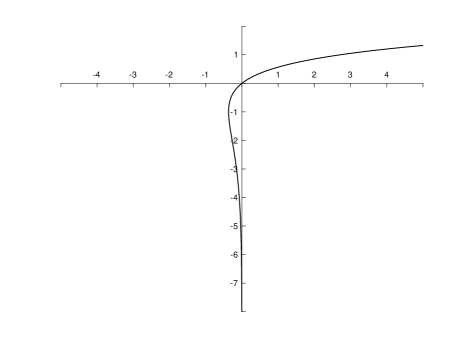
From the Lambert $W$ function, we know that $l\left(z\right)=ze^{z}=b$ has two real solutions when $b\in(-1/e,0)$ and one real solution when $b=-1/e$. As illustrated by Figure 18, if $0<c<1/e$, the two real solutions are $z_{1}=-a<-1$ and $z_{2}=m_{2}a>-1$; thus, $-1<m_{2}<0$. If $0<c<1/e$, the two real solutions are $-1<z_{1}=-a<0$ and $z_{2}=m_{2}a<-1$; thus, $m_{2}<-1$. If $c=1/e$, there is only one real solution $z_{1}=z_{2}=-1$; thus $m_{2}=m_{1}=-1$.

Figure 18: Lambert $W$ function.

It is important to note that in general an equation like $l\left(z\right)=ze^{z}=b$ has infinite complex roots. Let $z=\theta+i\eta$, and $b\in\left[-1/e,0\right)$. In that regard, we have

$$b =ze^{z}=\left(\theta+i\eta\right)e^{\theta+i\eta}$$

$$=\left(\theta+i\eta\right)\left(\cos\left(\eta\right)+i\sin\left(\eta\right)\right)$$

$$=\left(\theta\cos\left(\eta\right)-\eta\sin\left(\eta\right)\right)+i\left(\theta\sin\left(\eta\right)+\eta\cos\left(\eta\right)\right).$$

This implies that $\theta\sin\left(\eta\right)+\eta\cos\left(\eta\right)=0$, and $b=e^{\theta}\left(\theta\cos\left(\eta\right)-\eta\sin\left(\eta\right)\right)$, leading to

$$\eta=0,b=\theta e^{\theta}~{}~{}~{}\text{ or }~{}~{}~{}\theta=-\frac{\eta}{\tan\left(\eta\right)},b=-\frac{\eta\exp\left(-\frac{\eta}{\tan\left(\eta\right)}\right)}{\sin\left(\eta\right)}.$$

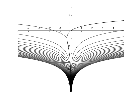
We plot the curves $b=\theta e^{\theta}$ and $\left(-\frac{\eta\exp\left(-\frac{\eta}{\tan\left(\eta\right)}\right)}{\sin\left(\eta\right)},-\frac{\eta}{\tan\left(\eta\right)}\right)$ to find out the relation between $b$ and the real part of the solution in Figure 19. The $x$-axis is $b$ and the $y$-axis is $\theta$. The blue curve is associated with $b=\theta e^{\theta}$, which is essentially the principle branch of the Lambert $W$ function. For any $b$, one can find the real values of the roots by fixing $b$. For instance, the green dashed line is associated with $b=-0.12$. As one can see, the curves intersect this line in infinite negative values. For $b\in[-1/e,0)$, we can see that the real roots are greater than the real part of the complex roots. For more explanation of this, see Siewert and Burniston (1973).

Figure 19: The real part of the Lambert $W$ roots.

Now assume that all the complex solutions for $\left(am\right)e^{am}=\left(-a\right)e^{\left(-a\right)}$ are $m_{k}=\lambda_{k}+\sigma_{k}i$ for $k=1,2,3,\dots$, where $(\lambda_{1},\sigma_{1})=(-1,0)$ and $(\lambda_{2},\sigma_{2})=(m_{2},0)$. Based on the above discussions, we have

$$\lambda_{1}=-1>\lambda_{2}=m_{2}>\lambda_{3}>\lambda_{4}>\dots\text{ when }c\in(1/e,1),$$

$$0>\lambda_{2}=m_{2}>\lambda_{1}=-1>\lambda_{3}>\lambda_{4}>\dots\text{ when }c\in(0,1/e),$$

and

$$\lambda_{1}=\lambda_{2}=-1>\lambda_{3}>\lambda_{4}>\dots\text{ when }c=1/e.$$

Let

$$\mathbb{C}=\left\{\begin{pmatrix}\lambda&-\sigma\\ \sigma&\lambda\\ \end{pmatrix}=\lambda+\sigma i\mid\lambda,\sigma\in\mathbb{R}\right\}$$

be the set of all complex numbers. Then,

$$x_{\mathbb{C}}(t)=\exp\left\{\begin{pmatrix}\lambda&-\sigma\\ \sigma&\lambda\\ \end{pmatrix}t\right\}$$

is a complex solution that solves (11). It is clear that (11) still holds for the linear transform of $x(t)$. Therefore, for any two $2\times 1$ vector $A$ and $B$,

$$x(t)=A^{\prime}x_{\mathbb{C}}(t)B=e^{\lambda t}\left(C_{1}\cos(\sigma t)+C_{2}\sin(\sigma t)\right)$$

is also a solution to (11).

In Bellman and Cooke (1963), it is shown that all complex solutions to (11) can be represented as follows:

$$x_{\mathbb{C}}\left(t\right)=\sum_{k=1}^{\infty}C_{k}e^{m_{k}t}.$$

Putting it in the real-valued context, we have that all real-valued solutions are in the following form:

$$x\left(t\right)=C_{1}e^{-t}+C_{2}e^{m_{2}t}+\sum_{k=3}^{\infty}e^{\lambda_{k}t}\left(C_{k,1}\cos\left(\sigma_{k}t\right)+C_{k,2}\sin\left(\sigma_{k}t\right)\right).$$

Now let us check $x^{\prime}+x>0$. This means that $C_{2}$, $\left\{C_{k,1}\right\}_{k\geqslant 3}$ and $\left\{C_{k,2}\right\}_{k\geqslant 3}$ for all $t$ must satisfy

$$x^{\prime}\left(t\right)+x\left(t\right)=\left(1+m_{2}\right)C_{2}e^{m_{2}t}\\ +\sum_{k=3}^{\infty}e^{\lambda_{k}t}\left(\left(\lambda_{k}C_{k,1}+\sigma_{k}C_{k,2}+C_{k,1}\right)\cos\left(\sigma_{k}t\right)+\left(\lambda_{k}C_{k,2}-\sigma_{k}C_{k,1}+C_{k,2}\right)\sin\left(\sigma_{k}t\right)\right)>0.$$

As $\lambda_{k}<m_{2}$ for $k\geqslant 3$, we have $\lim_{t\to\infty}\left(x^{\prime}(t)+x(t)\right)/e^{m_{2}t}=(1+m_{2})C_{2}$. Therefore, we need $C_{2}<0$ if $m_{2}<-1$ or $C_{2}>0$ if $m_{2}>-1$. That is $C_{2}(1+m_{2})>0$. Then the solution can be written as

$$x\left(t\right)=C_{1}e^{-t}+C_{2}e^{m_{2}t}+O\left(e^{\lambda_{3}t}\right).$$

By a change of variable, we get

$$f\left(y\right)=C_{1}+C_{2}y^{\alpha}+O\left(y^{\zeta}\right),$$

where $\alpha=-\left(1+m_{2}\right)$ and $\zeta=-\left(1+\lambda_{3}\right)$. As $\lambda_{3}<\min\{-1,m_{2}\}$ and $C_{2}(1+m_{2})>0$, we have $\zeta>\max\{0,\alpha\}$ and $C_{2}\alpha<0$. Also note that since $m_{2}$ solves $\left(am\right)e^{am}=\left(-a\right)e^{\left(-a\right)}$, by replacing $m_{2}=-1-\alpha$ and $a=-\log\left(c\right)$, we get ${(\alpha+1)^{-1/\alpha}}=c$. ∎

Appendix C Omitted proofs in Section 5

Proof of Proposition 4.

Before proving the statements in the proposition, we introduce the following linking function, for $X\in\mathcal{X}$,

$$\Gamma_{X}(\varepsilon)=1-F_{X}(\mathrm{ES}_{\varepsilon}(X)),~{}~{}~{}~{}\varepsilon\in[0,1].$$

As $X\in X$ it is easy to check that $\Gamma_{X}$ satisfies Assumption 1 for any $X\in\mathcal{X}$. The domain of $\Gamma_{X}(\varepsilon)$ is $[0,1]$ and its range is $[0,1-F_{X}(\mathbb{E}[X])]$.

As $\mathrm{ES}_{\varepsilon}(X)=\mathrm{VaR}_{\Gamma_{X}(\varepsilon)}(X)$, we have

$$\mathrm{VaR}_{\Gamma_{X}(\varepsilon)}(X)=\mathrm{ES}_{\varepsilon}(X)=\mathrm{VaR}_{\varepsilon/\pi_{X}(\varepsilon)}(X)\quad\text{for}\quad\varepsilon\in(0,1].$$

Hence we have the simple relationship $\Gamma_{X}(\varepsilon)=\varepsilon/\pi_{X}(\varepsilon).$ Therefore, $\Pi_{X}(\varepsilon)=\pi_{X}\left(\Gamma_{X}^{-1}(\varepsilon)\right)$ and $\pi_{X}(\varepsilon)=\Pi_{X}(\Gamma_{X}(\varepsilon))$. The function $\Gamma_{X}$ yields an association between a point on the PELVE on $(0,1-F_{X}(\mathbb{E}[X])]$ and a point on the dual PELVE curve on $(0,1]$ with the same value. Furthermore, we have $\pi_{X}$ is continuous on $(0,1)$ as $\pi_{X}(\varepsilon)=\varepsilon/\Gamma_{X}(\varepsilon)$ and $\Gamma_{X}$ is continuous.

Next, we show the statements (i)-(iv). The equivalence (i) of monotonicity of $\Pi_{X}$ and that of $\pi_{X}(\cdot)$ follows from $\Pi_{X}(\varepsilon)=\pi_{X}\left(\Gamma_{X}^{-1}(\varepsilon)\right)$, $\pi_{X}(\varepsilon)=\Pi_{X}(\Gamma_{X}(\varepsilon))$ and that $\Gamma_{X}$ is increasing.

For (ii), (iii) and (iv), we first show that $\Gamma_{X}$ is location-scale invariant and shape relevant (in the sense of (13)). Assume that $f:\mathbb{R}\to\mathbb{R}$ is a strictly increasing concave function such that $f(X)\in\mathcal{X}$. By Jensen’s inequality and the dual representation of $\mathrm{ES}_{p}$, we have

$$\mathrm{ES}_{p}\left(f(X)\right)\leqslant f\left(\mathrm{ES}_{p}(X)\right)$$

for all $p\in(0,1)$. This statement can be found in Appendices A.2 in Li and Wang (2022). Therefore,

$$\begin{array}[]{rl}&\Gamma_{f(X)}(\varepsilon)=1-F_{f(X)}\left(\mathrm{ES}_{\varepsilon}\left(f(X)\right)\right)\\ &\qquad\qquad\geqslant 1-F_{f(X)}\left(f\left(\mathrm{ES}_{\varepsilon}(X)\right)\right)=1-F_{X}\left(\mathrm{ES}_{\varepsilon}(X)\right)=\Gamma_{X}(\varepsilon).\end{array}$$ (13)

Then, we have $\Gamma_{f(X)}(\varepsilon)\geqslant\Gamma_{X}(\varepsilon)$ for all strictly increasing concave functions: $f:\mathbb{R}\to\mathbb{R}$ with $f(X)\in\mathcal{X}$.

For any strictly increasing convex function $g:\mathbb{R}\to\mathbb{R}$ with $g(X)\in\mathcal{X}$, we can take $f(x)=g^{-1}(X)$, which is a strictly increasing concave function. Therefore, we have $\Gamma_{g(X)}(\varepsilon)\leqslant\Gamma_{X}(\varepsilon)$ for all strictly increasing convex functions $g$.

For $\lambda>0$ and $a\in\mathbb{R}$, we have that $f(x)=\lambda X+a$ is both convex and concave. Therefore, $\Gamma_{\lambda X+a}(\varepsilon)=\Gamma_{X}(\varepsilon)$ for all $\varepsilon\in[0,1]$. In conclusion, we have the following results for $\Gamma$.

1. For all $\lambda>0$ and $a\in\mathbb{R}$, $\Gamma_{\lambda X+a}(\varepsilon)=\Gamma_{X}(\varepsilon)$.

2. $\Gamma_{f(X)}(\varepsilon)\geqslant\Gamma_{X}(\varepsilon)$ for all strictly increasing concave functions: $f:\mathbb{R}\to\mathbb{R}$ with $f(X)\in\mathcal{X}$.

3. $\Gamma_{g(X)}(\varepsilon)\leqslant\Gamma_{X}(\varepsilon)$ for all strictly increasing convex functions: $g:\mathbb{R}\to\mathbb{R}$ with $g(X)\in\mathcal{X}$.

Then, we have (ii), (iii) and (iv) from $\pi_{X}(\varepsilon)=\varepsilon/\Gamma_{X}(\varepsilon)$. ∎

Proof of Theorem 3.

The idea is to prove that if $1/\eta$ is convex (concave), then $x\mapsto F^{-1}((1-p)F(x)+p)$ is convex (concave) for all $p\in(0,1)$. Then, we can get the desired result by Proposition 5. We will use the following steps to show this statement.

Step 1. Let $s(x)=\log\left(1-F(x)\right)$ for $x\in(\mathrm{ess\mbox{-}inf}(X),\mathrm{ess\mbox{-}sup}(X))$. Then, $s$ is a continuous and strictly decreasing function and $s(x)<0$. Let $s^{-1}$ be the inverse function of $s$. Now, we have

$$F(x)=1-e^{s(x)},\quad x\in(\mathrm{ess\mbox{-}inf}(X),\mathrm{ess\mbox{-}sup}(X))$$

and

$$F^{-1}(t)=s^{-1}(\log(1-t)),\quad t\in(0,1).$$

Therefore,

$$F^{-1}\big{(}(1-p)F(x)+p\big{)} =s^{-1}\big{(}\log(1-(1-p)F(x)-p)\big{)}$$

$$=s^{-1}\Big{(}\log\big{(}1-F(x)\big{)}+\log(1-p)\Big{)}$$

$$=s^{-1}\Big{(}\log\big{(}e^{s(x)}\big{)}+\log(1-p)\Big{)}$$

$$=s^{-1}\Big{(}s(x)+\log(1-p)\Big{)}.$$

Let $\theta=\log(1-p)$. It follows that the statement that $x\mapsto F^{-1}\big{(}(1-p)F(x)+p\big{)}$ is convex (concave) for all $p\in(0,1)$ is equivalent to the statement that $x\mapsto s^{-1}\left(s(x)+\theta\right)$ is convex (concave) for all $\theta<0$.

Step 2. Let $g(x):=-s^{-1}(x)$. Then, $g$ is strictly increasing. We will show that if $1/\eta$ is convex (concave), $\log(g^{\prime}(x))$ is convex (concave).

As $g(x)=-s^{-1}(x)=-S^{-1}(e^{x}),$ we have

$$g^{\prime}(x)=\frac{e^{x}}{f\left(S^{-1}(e^{x})\right)}.$$

Let $H(x):=\log(g^{\prime}(x))=x-\log\left(f\left(S^{-1}(e^{x})\right)\right)$. We have

$$H\left(\log(S(x))\right)=\log S(x)-\log f(x)=-\log\eta(x).$$ (14)

Then, taking the derivative on both sides of (14), we get

$$-H^{\prime}\big{(}\log(S(x))\big{)}\eta(x)=-\frac{\eta^{\prime}(x)}{\eta(x)}$$

$$\Longleftrightarrow{}{} H^{\prime}\big{(}\log(S(x))\big{)}=\frac{\eta^{\prime}(x)}{\eta^{2}(x)}=-\frac{\mathrm{d}}{\mathrm{d}x}\left(\frac{1}{\eta(x)}\right).$$

Taking a derivative in both sides again, we get

$$-H^{\prime\prime}\big{(}\log(S(x))\big{)}\eta(x)=-\frac{\mathrm{d}^{2}}{\mathrm{d}x^{2}}\left(\frac{1}{\eta(x)}\right).$$

Then, $1/\eta$ is a convex (concave) function means $H^{\prime\prime}(x)\geqslant 0$ ($H^{\prime\prime}(x)\leqslant 0$), which gives that $\log g^{\prime}(x)$ is convex (concave).

Step 3. For $\theta<0$, let $G_{\theta}(x):=s^{-1}(s(x)+\theta)$. We are going to show

$$\lim_{z\to 0}\frac{G_{\theta}(x+z)-G_{\theta}(x)}{z}\leqslant\lim_{z\to 0}\frac{G_{\theta}(x^{\prime}+z)-G_{\theta}(x^{\prime})}{z}$$ (15)

for all $x<x^{\prime}$.

We take $z>0$ first. As $s$ is strictly decreasing, $s^{-1}$ is also strictly decreasing. Then, $G_{\theta}$ is a continuous and strictly increasing function. As $\theta<0$, we also have $G_{\theta}(x)>x$. Take arbitrary $x,x^{\prime},y$ and $z$ such that $x<x^{\prime}$, $x<y$ and $z>0$. Let $\theta=s(y)-s(x)$. Then, we have $G_{\theta}(x)=y$. Define

$$h=G_{\theta}(x+z)-y,\quad y^{\prime}=G_{\theta}(x^{\prime})\quad\text{and}\quad h^{\prime}=G_{\theta}(x^{\prime}+z)-y^{\prime}.$$

By the definition of $G_{\theta}$, we have $s(y+h)=s(x+z)+\theta$, $s(y^{\prime})=s(x^{\prime})+\theta$ and $s(y^{\prime}+h^{\prime})=s(x^{\prime}+z)+\theta$. As a result, we have

$$s(y+h)-s(y)=s(x+z)-s(x)\quad\text{and}\quad s(y^{\prime}+h^{\prime})-s(y^{\prime})=s(x^{\prime}+z)-s(x^{\prime}).$$

By the mean-value theorem, there exists $\zeta\in(y,y+h)$, $\zeta^{\prime}\in(y^{\prime},y^{\prime}+h^{\prime})$, $\xi\in(x,x+z)$ and $\xi^{\prime}\in(x^{\prime},x^{\prime}+z)$ such that

$$s^{\prime}(\zeta)h=s^{\prime}(\xi)z\text{ and }s^{\prime}(\zeta^{\prime})h^{\prime}=s^{\prime}(\xi^{\prime})z.$$

Furthermore, $x,x^{\prime},y$ and $y^{\prime}$ satisfy $x<x^{\prime}<y^{\prime}$ and $x<y<y^{\prime}$. If $z$ is small enough, then $h$ and $h^{\prime}$ will also be small enough as $G_{\theta}$ is continuous. Therefore, we have $\xi<\xi^{\prime}<\zeta^{\prime}$ and $\xi<\zeta<\zeta^{\prime}$ when $z$ is small enough.

In Step 2, we have that $\log g^{\prime}(x)$ is convex when $1/\eta$ is convex. Therefore, we get

$$\log(g^{\prime}(a))+\log(g^{\prime}(b))\geqslant\log(g^{\prime}(a^{\prime}))+\log(g^{\prime}(b^{\prime})),$$

for all $a<a^{\prime}<b$ and $a<b^{\prime}<b$, which means

$$g^{\prime}(a)g^{\prime}(b)\geqslant g^{\prime}(a^{\prime})g^{\prime}(b^{\prime}).$$

As $g(x)=-s^{-1}(x)$, we have

$$\frac{1}{s^{\prime}(s^{-1}(a))s^{\prime}(s^{-1}(b))}\geqslant\frac{1}{s^{\prime}(s^{-1}(a^{\prime}))s^{\prime}(s^{-1}(b^{\prime}))}.$$

As $s^{-1}(x)$ is strictly decreasing, it means that

$$s^{\prime}(\alpha)s^{\prime}(\beta)\leqslant s^{\prime}(\alpha^{\prime})s^{\prime}(\beta^{\prime})$$

for $\alpha>\alpha^{\prime}>\beta$ and $\alpha>\beta^{\prime}>\beta$. Therefore, we have $s^{\prime}(\xi)s^{\prime}(\zeta^{\prime})\leqslant s^{\prime}(\xi^{\prime})s^{\prime}(\zeta)$ as $\zeta^{\prime}>\zeta>\xi$ and $\zeta^{\prime}>\xi^{\prime}>\xi$. That is,

$$h=\frac{s^{\prime}(\xi)z}{s^{\prime}(\zeta)}\leqslant\frac{s^{\prime}(\xi^{\prime})z}{s^{\prime}(\zeta^{\prime})}=h^{\prime}.$$

On the other hand, $h=G_{\theta}(x+z)-G_{\theta}(x)$ and $h^{\prime}=G_{\theta}(x^{\prime}+z)-G_{\theta}(x^{\prime})$. Therefore,

$$G_{\theta}(x+z)-G_{\theta}(x)\leqslant G_{\theta}(x^{\prime}+z)-G_{\theta}(x^{\prime})$$

when $z$ is small enough. If $z<0$, we can also get (15) by an analogous argument.

Hence, the second-order derivative of $G_{\theta}$ is increasing for each $\theta<0$, which means that $x\mapsto F^{-1}\big{(}(1-p)F(x)+p\big{)}$ is convex for all $p\in(0,1)$ if $1/\eta$ is convex.

An analogous argument yields that $x\mapsto F^{-1}\big{(}(1-p)F(x)+p\big{)}$ is concave for all $p\in(0,1)$ when $1/\eta$ is concave. ∎

References

- Acerbi and Székely (2014) Acerbi, C. and Székely, B. (2014). Backtesting expected shortfall. Risk, 27(11), 76-81.
- Artzner et al. (1999) Artzner, P., Delbaen, F., Eber, J.-M. and Heath, D. (1999). Coherent measures of risk. Mathematical Finance, 9(3), 203–228.
- Balbás et al. (2017) Balbás, A., Balbás, B. and Balbás, R. (2017). Differential equations connecting VaR and CVaR. Journal of Computational and Applied Mathematics, 326, 247–267.
- Barczy et al. (2022) Barczy, M., Nedényi, F. K. and Sütő, L. (2022). Probability equivalent level of Value at Risk and higher-order Expected Shortfalls. Insurance: Mathematics and Economics, 108, 107–128.
- BCBS (2019) BCBS (2019). Minimum Capital Requirements for Market Risk. February 2019. Basel Committee on Banking Supervision. Basel: Bank for International Settlements. BIS online publication No. bcbs457.
- Behan et al. (2010) Behan, D. F., Cox, S. H., Lin, Y., Pai, J., Pedersen, H. W. and Yi, M. (2010). Obesity and its relation to mortality and morbidity costs. Society of Actuaries, 59.
- Bellman and Cooke (1963) Bellman, R. and Cooke, K. L. (1963). Differential-difference Equations. Academic Press, New York.
- Berezansky and Braverman (2011) Berezansky, L. and Braverman, E. (2011). On nonoscillation of advanced differential equations with several terms. Abstract and Applied Analysis, 2011, 637142.
- Chambers (2009) Chambers, C. P. (2009). An axiomatization of quantiles on the domain of distribution functions. Mathematical Finance, 19(2), 335–342.
- Cont et al. (2010) Cont, R., Deguest, R. and Scandolo, G. (2010). Robustness and sensitivity analysis of risk measurement procedures. Quantitative Finance, 10(6), 593–606.
- Embrechts and Hofert (2013) Embrechts, P. and Hofert, M. (2013). A note on generalized inverses. Mathematical Methods of Operations Research, 77(3), 423–432.
- Embrechts et al. (2016) Embrechts, P., Hofert, M. and Wang, R. (2016). Bernoulli and tail-dependence compatibility. Annals of Applied Probability, 26(3), 1636–1658.
- Embrechts et al. (2018) Embrechts, P., Liu, H. and Wang, R. (2018). Quantile-based risk sharing. Operations Research, 66(4), 936–949.
- Embrechts et al. (2002) Embrechts, P., McNeil, A. and Straumann, D. (2002). Correlation and dependence in risk management: properties and pitfalls. Risk Management: Value at Risk and Beyond, 1, 176–223.
- Embrechts et al. (2014) Embrechts, P., Puccetti, G., Ruschendorf, L., Wang, R. and Beleraj, A. (2014). An academic response to Basel 3.5. Risks, 2(1), 25–48.
- Emmer et al. (2015) Emmer, S., Kratz, M. and Tasche, D. (2015). What is the best risk measure in practice? A comparison of standard measures. Journal of Risk, 18(2), 31–60.
- Fiori and Rosazza Gianin (2023) Fiori, A. M. and Rosazza Gianin, E. (2023). Generalized PELVE and applications to risk measures. European Actuarial Journal, 13(1), 307-339.
- Frees (2009) Frees, E. W. (2009). Regression Modeling with Actuarial and Financial Applications. Cambridge University Press. Cambridge.
- Gneiting (2011) Gneiting, T. (2011). Making and evaluating point forecasts. Journal of the American Statistical Association, 106(494), 746–762.
- Krause et al. (2018) Krause, D., Scherer, M., Schwinn, J. and Werner, R. (2018). Membership testing for Bernoulli and tail-dependence matrices. Journal of Multivariate Analysis, 168, 240–260.
- Kou and Peng (2016) Kou, S. and Peng, X. (2016). On the measurement of economic tail risk. Operations Research, 64(5), 1056–1072.
- Li and Wang (2022) Li, H. and Wang, R. (2022). PELVE: Probability equivalent level of VaR and ES. Journal of Econometrics, 234(1), 353–370.
- Liu and Wang (2021) Liu, F. and Wang, R. (2021). A theory for measures of tail risk. Mathematics of Operations Research, 46(3), 1109–1128.
- McNeil et al. (2015) McNeil, A. J., Frey, R. and Embrechts, P. (2015). Quantitative Risk Management: Concepts, Techniques and Tools. Revised Edition. Princeton, NJ: Princeton University Press.
- Rudin (1987) Rudin, W. (1987). Real and Complex Analysis. International Series in Pure and Applied Mathematics (3rd Ed.). McGraw–Hill. New York.
- Siewert and Burniston (1973) Siewert, C. E. and Burniston, E. E. (1973). Exact analytical solutions of . Journal of Mathematical Analysis and Applications, 43(3), 626–632.
- Wang and Zitikis (2021) Wang, R. and Zitikis, R. (2021). An axiomatic foundation for the Expected Shortfall. Management Science, 67, 1413–1429.