\newsiamremark

remarkRemark \newsiamremarkhypothesisHypothesis \newsiamthmclaimClaim \headersIntegral Fractional Laplacian in Multiple Dimensions C. Sheng, B. Su, and C. Xu

Efficient Monte Carlo Method for Integral Fractional Laplacian in Multiple Dimensions thanks: Submitted to the editors DATE. \fundingThe research of the first author is partially supported by Shanghai Pujiang Program 21PJ1403500, the Fundamental Research Funds for the Central Universities 2021110474 and Shanghai Post-doctoral Excellence Program 2021154. The research of the third author is partially supported by he Fundamental Research Funds for the Central Universities.

Changtao Sheng School of Mathematics, Shanghai University of Finance and Economics, Shanghai 200433, China. Email: (C. Sheng); (B. Su); (C. Xu). ctsheng@sufe.edu.cn subihao@163.sufe.edu.cn xu.chenglong@shufe.edu.cn    Bihao Su    Chenglong Xu
Abstract

In this paper, we develop a Monte Carlo method for solving PDEs involving an integral fractional Laplacian (IFL) in multiple dimensions. We first construct a new Feynman-Kac representation based on the Green function for the fractional Laplacian operator on the unit ball in arbitrary dimensions. Inspired by the “walk-on-spheres” algorithm proposed in [24], we extend our algorithm for solving fractional PDEs in the complex domain. Then, we can compute the expectation of a multi-dimensional random variable with a known density function to obtain the numerical solution efficiently. The proposed algorithm finds it remarkably efficient in solving fractional PDEs: it only needs to evaluate the integrals of expectation form over a series of inside ball tangent boundaries with the known Green function. Moreover, we carry out the error estimates of the proposed method for the n𝑛n-dimensional unit ball. Finally, ample numerical results are presented to demonstrate the robustness and effectiveness of this approach for fractional PDEs in unit disk and complex domains, and even in ten-dimensional unit balls.

keywords:
Integral fractional Laplacian, Green function, Monte Carlo method, Spherical coordinate
{AMS}

37P30, 60G22, 65C05, 65L70, 91G60

1 Introduction

Fractional powers of the Laplacian operator are a powerful tool in modeling phenomena in anomalous diffusion, which arise naturally in the α𝛼\alpha-stable Le´´e\acute{\text{e}}vy process instead of the Brownian motion for normal diffusion (see, e.g., [35, 27, 28, 7] and the references therein). It is known that for α(0,2),𝛼02\alpha\in(0,2), the fractional Laplacian of a sufficiently nice function u(𝒙):n:𝑢𝒙superscript𝑛u(\bm{x})\!:\mathbb{R}^{n}\to\mathbb{R} has the hypersingular integral representation (cf.​ [30]):

(1) (Δ)α2u(𝒙)=Cn,αp.v.nu(𝒙)u(𝒚)|𝒙𝒚|n+αd𝒚,Cn,α:=2αΓ(n+α2)πn2Γ(1α2),formulae-sequencesuperscriptΔ𝛼2𝑢𝒙subscript𝐶𝑛𝛼pvassignsubscriptsuperscript𝑛𝑢𝒙𝑢𝒚superscript𝒙𝒚𝑛𝛼differential-d𝒚subscript𝐶𝑛𝛼superscript2𝛼Γ𝑛𝛼2superscript𝜋𝑛2Γ1𝛼2(-\Delta)^{\frac{\alpha}{2}}u(\bm{x})=C_{n,\alpha}\,{\rm p.v.}\!\int_{\mathbb{R}^{n}}\frac{u(\bm{x})-u(\bm{y})}{|\bm{x}-\bm{y}|^{n+\alpha}}\,{\rm d}\bm{y},\quad C_{n,\alpha}:=\frac{2^{\alpha}\Gamma(\frac{n+\alpha}{2})}{\pi^{\frac{n}{2}}\Gamma(1-\frac{\alpha}{2})},

where “p.v.” stands for the principle value and Cn,αsubscript𝐶𝑛𝛼C_{n,\alpha} is the normalisation constant. This point-wise expression for the fractional Laplacian can directly be derived from the following Fourier transform:

(2) (Δ)α2u(𝒙)=1[|𝝃|α[u](𝝃)](𝒙),𝒙n.formulae-sequencesuperscriptΔ𝛼2𝑢𝒙superscript1delimited-[]superscript𝝃𝛼delimited-[]𝑢𝝃𝒙𝒙superscript𝑛\begin{split}(-\Delta)^{\frac{\alpha}{2}}u(\bm{x})={\mathscr{F}}^{-1}\big{[}|\bm{\xi}|^{\alpha}{\mathscr{F}}[u](\bm{\xi})\big{]}(\bm{x}),\;\;\bm{x}\in{\mathbb{R}}^{n}.\end{split}

The nonlocal and singular nature of this operator poses major difficulties in discretisation and analysis. In the case where α=2𝛼2\alpha=2 the operator coincides with the usual negative Laplacian ΔΔ-\Delta. Most recent concerns are with PDEs involving the IFL operator on an open bounded Lipschitz domain Ωn.Ωsuperscript𝑛\Omega\subset\mathbb{R}^{n}. More precisely, given f:Ω:𝑓Ωf:\Omega\to\mathbb{R} in a suitable space, we look for u𝑢u on ΩΩ\Omega satisfying the fractional Poisson equation with the (nonlocal) Dirichlet boundary condition:

(3) {(Δ)α2u(𝒙)=f(𝒙),inΩ,u(𝒙)=g(𝒙),onΩc:=n\Ω.casessuperscriptΔ𝛼2𝑢𝒙𝑓𝒙inΩ𝑢𝒙𝑔𝒙assignonsuperscriptΩ𝑐\superscript𝑛Ω\begin{cases}(-\Delta)^{\frac{\alpha}{2}}u(\bm{x})=f(\bm{x}),\;&{\rm in}\ \Omega,\\[4.0pt] u(\bm{x})=g(\bm{x}),\quad&{\rm on}\ \Omega^{c}:=\mathbb{R}^{n}\backslash\Omega.\end{cases}

1.1 Review on existing studies

The numerical method for fractional Poisson equation (3) is challenging due to the nonlocality of the fractional Laplacian operator, hyper-singular integrals, and the low regularity of the solution at the boundary. In general, the existing approaches can be classified into the following two categories.

The first is to discretize the fractional Poisson equations using demerministic numerical methods. It is customary to apply finite difference methods for integral fractional Laplacian (see, e.g., [14, 15, 29, 23] and many references therein). However, those finite difference discretizations are only available for simple domains such as rectangular domains and require stronger regularity assumptions for the solution. The finite element methods are more preferable for solving fractional PDEs, as it has a well-established theoretical foundation and the capability to deal with complex domain. The IFL operator has interwoven connections with the fractional Sobolev framework (cf.​ [30]), so the finite element scheme can be established under more realistic assumptions, i.e., in fractional Sobolev space and without additional regularity requirements. There have been many recent works devoted to the FEM analysis for fractional PDEs (see, e.g., [1, 2, 5, 4, 6, 17] and the references therein), but the literature on FEM implementation in multiple dimensions is very limited. Compared with the local schemes, the special designed spectral methods could compensate for the weakly singular behavior of the solution and hence are expected to approximate the solution of (3) accurately. However, the spectral methods are limited to one dimension, simple domains, and the whole space case, we refer to [26, 36, 34, 10, 22, 21] and the references therein for more details. Needless to say, for IFL on the bounded domain, these methods become complicated even for n=2,3𝑛23n=2,3 and computationally prohibitive for the higher-dimensional cases.

The second is to use Monte Carlo methods based on the stochastic processes to alleviate its proverbial numerical difficulties. It is well-known that the Feynman-Kac formula is an important bridge to link PDEs and stochastic processes (see, e.g., [11, 12, 18, 24, 38] and the references therein), which offers a method of solving certain PDEs via simulating random paths of a stochastic process. For the classical Poisson equations, that is,

(4) Δu(𝒙)=f(𝒙)inΩ;u(𝒙)=g(𝒙)onΩ,formulae-sequenceΔ𝑢𝒙𝑓𝒙inΩ𝑢𝒙𝑔𝒙onΩ-\Delta u(\bm{x})=f(\bm{x})\quad{\rm in}\;\;\Omega;\quad u(\bm{x})=g(\bm{x})\quad{\rm on}\;\;\partial\Omega,

which is governed by Brownian motion and the solution (4) has a Feynman-Kac representation, expressed as an expectation at first exit from ΩΩ\Omega of the associated Wiener process (cf. [13]). Remarkably, in [13, 24], the Feynman-Kac representation was extended to fractional Laplacian, where Brownian motion was replaced by α𝛼\alpha-stable Le´´e\acute{\text{e}}vy process. Let ΩnΩsuperscript𝑛\Omega\subset\mathbb{R}^{n} be a bounded domain, with n1𝑛1n\geq 1. For any α(0,2)𝛼02\alpha\in(0,2) and a Borel set ΛnΛsuperscript𝑛\Lambda\subset\mathbb{R}^{n}, we denote

Lα1(Λ)={uL1(Λ)s.t.Λ|u(x)|1+|x|n+αdx<}.L^{1}_{\alpha}(\Lambda)=\Big{\{}u\in L^{1}(\Lambda)\;\;{\rm s.t.}\;\int_{\Lambda}\frac{|u(x)|}{1+|x|^{n+\alpha}}\,{\rm d}x<\infty\Big{\}}.

Suppose that g(x)𝑔𝑥g(x) is a continuous function that belongs to Lα1(Ωc)subscriptsuperscript𝐿1𝛼superscriptΩ𝑐L^{1}_{\alpha}(\Omega^{c}), and f(x)𝑓𝑥f(x) is a function in Cα+ϵ(Ω)superscript𝐶𝛼italic-ϵΩC^{\alpha+\epsilon}(\Omega) for some ϵ>0italic-ϵ0\epsilon>0. Then there exists a unique continuous solution to problem (3) in Lα1(n)subscriptsuperscript𝐿1𝛼superscript𝑛L^{1}_{\alpha}(\mathbb{R}^{n}), which is given by (see [24, Thm. 6.1])

(5) u(x)=𝔼X0α=x[g(XτΩα)]+𝔼X0α=x[0τΩf(Xsα)ds],xΩ,formulae-sequence𝑢𝑥subscript𝔼superscriptsubscript𝑋0𝛼𝑥delimited-[]𝑔subscriptsuperscript𝑋𝛼subscript𝜏Ωsubscript𝔼superscriptsubscript𝑋0𝛼𝑥delimited-[]superscriptsubscript0subscript𝜏Ω𝑓subscriptsuperscript𝑋𝛼𝑠differential-d𝑠𝑥Ωu(x)=\mathbb{E}_{X_{0}^{\alpha}=x}\big{[}g(X^{\alpha}_{\tau_{\Omega}})\big{]}+\mathbb{E}_{X_{0}^{\alpha}=x}\Big{[}\int_{0}^{\tau_{\Omega}}f(X^{\alpha}_{s})\,{\rm d}s\Big{]},\;\;x\in\Omega,

where τΩ=inf{t>0:XtαΩ}subscript𝜏Ωinfimumconditional-set𝑡0superscriptsubscript𝑋𝑡𝛼Ω\tau_{\Omega}=\inf\{t>0:X_{t}^{\alpha}\notin\Omega\}, and {Xtα}t0subscriptsuperscriptsubscript𝑋𝑡𝛼𝑡0\{X_{t}^{\alpha}\}_{t\geq 0} is a symmetric α𝛼\alpha-stable Le´´e\acute{\text{e}}vy process with X0α=xsuperscriptsubscript𝑋0𝛼𝑥X_{0}^{\alpha}=x. We recall that a stochastic process {Xtα;t0}superscriptsubscript𝑋𝑡𝛼𝑡0\{X_{t}^{\alpha};t\geq 0\} is called symmetric α𝛼\alpha-stable Le´´e\acute{\text{e}}vy process if:

(1). X0α=0subscriptsuperscript𝑋𝛼00X^{\alpha}_{0}=0 a.s.;

(2). Xtαsubscriptsuperscript𝑋𝛼𝑡X^{\alpha}_{t} has independent and stationary increments;

(3). XtαXsαSα((ts)1/α,0,0)subscriptsuperscript𝑋𝛼𝑡subscriptsuperscript𝑋𝛼𝑠subscript𝑆𝛼superscript𝑡𝑠1𝛼00X^{\alpha}_{t}-X^{\alpha}_{s}\backsim S_{\alpha}((t-s)^{1/\alpha},0,0) for any 0s<t<0𝑠𝑡0\leq s<t<\infty, that is, α𝛼\alpha-stable distribution with

scale parameter (ts)1/αsuperscript𝑡𝑠1𝛼(t-s)^{1/\alpha}, and skewness and shift parameters equal to zero.

In particular, when α=2𝛼2\alpha=2, then Xt2=2Btsuperscriptsubscript𝑋𝑡22subscript𝐵𝑡X_{t}^{2}=\sqrt{2}B_{t}, Btsubscript𝐵𝑡B_{t} represents the standard Brownian motion. The symmetric α𝛼\alpha-stable Le´´e\acute{\text{e}}vy process is 1/α1𝛼1/\alpha self-similar. That is for k>0𝑘0k>0, the process {Xktα;t0}subscriptsuperscript𝑋𝛼𝑘𝑡𝑡0\{X^{\alpha}_{kt};t\geq 0\} and {k1/αXtα;t0}superscript𝑘1𝛼subscriptsuperscript𝑋𝛼𝑡𝑡0\{k^{1/\alpha}X^{\alpha}_{t};t\geq 0\} have the same finite-dimensional distributions. The characteristic function (see [3]) of a α𝛼\alpha-stable random variable X𝑋X is given by

(6) lnψ(θ)={σα|θ|α[1iβsgn(θ)tan(απ2)+iμθ],ifα(0,1)(1,2],σ|θ|[1+iβ2πsgn(θ)ln|θ|+iμθ],ifα=1,𝜓𝜃casessuperscript𝜎𝛼superscript𝜃𝛼delimited-[]1i𝛽sgn𝜃𝛼𝜋2i𝜇𝜃if𝛼0112𝜎𝜃delimited-[]1i𝛽2𝜋sgn𝜃𝜃i𝜇𝜃if𝛼1\displaystyle\ln\psi(\theta)=\begin{cases}-\sigma^{\alpha}|\theta|^{\alpha}\big{[}1-\mathrm{i}\beta\text{sgn}(\theta)\tan(\frac{\alpha\pi}{2})+\mathrm{i}\mu\theta\big{]},&{\rm if}~{}\alpha\in(0,1)\cup(1,2],\\[4.0pt] -\sigma|\theta|\big{[}1+\mathrm{i}\beta\frac{2}{\pi}\text{sgn}(\theta)\ln|\theta|+\mathrm{i}\mu\theta\big{]},&{\rm if}~{}\alpha=1,\end{cases}

where α(0,2]𝛼02\alpha\in(0,2] is the index of stability, β[1,1]𝛽11\beta\in[-1,1] denotes the skewness parameter, μ𝜇\mu\in\mathbb{R} and σ>0𝜎0\sigma>0 represent the shift and scale parameters respectively. Then X𝑋X is called α𝛼\alpha-random variable, and we use the notation XSα(σ,β,μ)𝑋subscript𝑆𝛼𝜎𝛽𝜇X\backsim S_{\alpha}(\sigma,\beta,\mu). Obviously, S1(σ,0,μ)subscript𝑆1𝜎0𝜇S_{1}(\sigma,0,\mu) and S2(σ,0,μ)subscript𝑆2𝜎0𝜇S_{2}(\sigma,0,\mu) are the Cauchy distribution and the Gaussian distribution 𝒩(μ,σ)𝒩𝜇𝜎\mathcal{N}(\mu,\sigma), respectively (cf. [3]).

This groundbreaking representation provides a viable alternative for its mathematical and numerical treatment. Kyprianou et al. [24] developed an efficient Monte Carlo method for (3) in two dimensions by using the walk-on-spheres algorithm, which is based on the Feynman-Kac representation. With this idea, Shardlow [33] proposed the multilevel Monte Carlo method combined with the Walk outside spheres algorithm for solving the eigenvalues problem involving fractional Laplacian operator. Those methods can be extended to high-dimensional cases. However, it will become complicated, as the Feynman-Kac representation is associated with a high dimensional α𝛼\alpha-stable process, which seems not an easy task. Thus, extending those approaches to a higher dimensional case is nontrivial.

We also remark that direct learning of the IFL and/or nonlocal models on bounded domains was discussed in some recent works (see, e.g., [31, 9] for Physical-informed neural networks (PINN); and [32, 19, 25, 37, 20] for deep learning methods). We note that most current works tend to combine the traditional automatic differential method with some typical numerical discretization to solve the fractional or nonlocal models.

1.2 Our contributions and the organization of the paper

This paper proposes and analyzes a Monte Carlo method for PDEs involving integral fractional Laplacian on the bounded domain in arbitrary dimensions. The proposed method takes advantage of the Feynman-Kac representation based on Green functions for the simulation of both classical and fractional Laplacians in a unified framework, which avoids the enormous computational cost of evaluating the fractional derivatives. We highlight below the main advantages of the proposed methods and main contributions of the paper:

  • We provide a new Feynman-Kac representation for the solution of fractional Poisson equations on the ball in arbitrary dimensions (see Lemma 2.3 below). Benefiting from the new representation, to avoid calculating the expectation of a complex integral that involves the function of α𝛼\alpha-stable Lévy process, we can evaluate the expectation of a random variable associated with the explicit expression of the Green functions to obtain the solution.

  • We further extended the representation for fractional PDEs on the irregular domain. More precisely, as shown in Theorem 2.6 of this paper, the solution of (3) on an open bounded domain can be evaluated by the expectation of a sequence of inside balls tangent to the boundary, as the Green’s function and Poisson’s kernel on the balls are known. The existing work [24] is to adopt the walk-on-spheres algorithm for solving fractional Poisson equation in two dimensions, in which the walk-on-spheres precess is associated with the α𝛼\alpha-stable process.

  • The proposed method is capable of fractional PDEs in high dimensions. Moreover, in the Monte Carlo procedure, thanks to spherical coordinates, the distribution in the angular direction for each jump is uniform, allowing us only need to appropriately increase the samples in the angular direction with the increase of dimensionality so that the computation time will increase at a moderate pace.

  • We fully analyze the error analysis and characterize the efficiency of the proposed method for fractional Poisson equations on the ball in arbitrary dimensions, with the aid of the property of the Monte Carlo procedure and the explicit expressions of the Green functions.

The rest of the paper is organized as follows. In the next section, we derive an alternative formula based on the Green function of integral fractional Laplacian operator on the unit ball in arbitrary dimensions and extend the result to the case of irregular domain. Section 3 describes the detailed algorithm for computing the fractional PDEs based on the Monte Carlo method. In Section 4, we provide a complete error analysis of the proposed methods for the fractional Poisson equation. Numerical experiments for PDEs with integral fractional Laplacian are carried out in Section 5. Some concluding remarks are given in the last section.

2 Main results

2.1 Feynman-Kac representation in expectation form in a ball

In this section, we introduce some representation formula for the solution of fractional Laplacian operator on the ball in arbitrary dimensions. To this ends, we set 𝒄0nsubscript𝒄0superscript𝑛\bm{c}_{0}\in\mathbb{R}^{n} and define r>0𝑟0r>0 to be the radius of a ball inscribed in nsuperscript𝑛\mathbb{R}^{n} that is centered at 𝒄0subscript𝒄0\bm{c}_{0}. This sphere we will call 𝔹rn,𝒄0={𝒙n:|𝒙𝒄0|r}subscriptsuperscript𝔹𝑛subscript𝒄0𝑟conditional-set𝒙superscript𝑛𝒙subscript𝒄0𝑟\mathbb{B}^{n,\bm{c}_{0}}_{r}=\{\bm{x}\in\mathbb{R}^{n}:|\bm{x}-\bm{c}_{0}|\leq r\}. Let 𝔹rn=𝔹rn,𝟎superscriptsubscript𝔹𝑟𝑛superscriptsubscript𝔹𝑟𝑛0\mathbb{B}_{r}^{n}=\mathbb{B}_{r}^{n,\bm{0}} for simplicity.

We first show that the solution of (3) on the ball can be explicitly represented as the following integral form as follows, which play important role in the algorithm development.

Lemma 2.1.

Let r>0𝑟0r>0 and α(0,2]𝛼02\alpha\in(0,2]. If fLα1(𝔹rn)C(𝔹¯rn)𝑓subscriptsuperscript𝐿1𝛼superscriptsubscript𝔹𝑟𝑛𝐶superscriptsubscript¯𝔹𝑟𝑛f\in L^{1}_{\alpha}(\mathbb{B}_{r}^{n})\cap C(\overline{\mathbb{B}}_{r}^{n}), gLα1(n𝔹rn)𝑔subscriptsuperscript𝐿1𝛼superscript𝑛superscriptsubscript𝔹𝑟𝑛g\in L^{1}_{\alpha}(\mathbb{R}^{n}\!\setminus\!\mathbb{B}_{r}^{n}), then the solution of (3) with Ω=𝔹rnΩsubscriptsuperscript𝔹𝑛𝑟\Omega=\mathbb{B}^{n}_{r} can be represented as

(7) u(𝒙)={𝔹rnf(𝒚)Qr(𝒙,𝒚)d𝒚+n𝔹rng(𝒛)Pr(𝒙,𝒛)d𝒛,in𝔹rn,g(𝒙),onn𝔹rn,𝑢𝒙casessubscriptsubscriptsuperscript𝔹𝑛𝑟𝑓𝒚subscript𝑄𝑟𝒙𝒚differential-d𝒚subscriptsuperscript𝑛subscriptsuperscript𝔹𝑛𝑟𝑔𝒛subscript𝑃𝑟𝒙𝒛differential-d𝒛insubscriptsuperscript𝔹𝑛𝑟𝑔𝒙onsuperscript𝑛subscriptsuperscript𝔹𝑛𝑟u(\bm{x})=\begin{cases}\displaystyle\int_{\mathbb{B}^{n}_{r}}f(\bm{y})Q_{r}(\bm{x},\bm{y})\,\mathrm{d}\bm{y}+\displaystyle\int_{\mathbb{R}^{n}\setminus\mathbb{B}^{n}_{r}}g(\bm{z})P_{r}(\bm{x},\bm{z}){\rm d}\bm{z},&{\rm in}\,\mathbb{B}^{n}_{r},\\[6.0pt] g(\bm{x}),&{\rm on}\,\mathbb{R}^{n}\!\setminus\!\mathbb{B}^{n}_{r},\end{cases}

where Pr(𝐱,𝐳)subscript𝑃𝑟𝐱𝐳P_{r}(\bm{x},\bm{z}) is the Poisson kernel defined by

(8) Pr(𝒙,𝒛)=C~nα(r2|𝒙|2|𝒛|2r2)α/21|𝒙𝒛|n,𝒙𝔹rn,𝒛n𝔹¯rn,formulae-sequencesubscript𝑃𝑟𝒙𝒛subscriptsuperscript~𝐶𝛼𝑛superscriptsuperscript𝑟2superscript𝒙2superscript𝒛2superscript𝑟2𝛼21superscript𝒙𝒛𝑛formulae-sequence𝒙subscriptsuperscript𝔹𝑛𝑟𝒛superscript𝑛subscriptsuperscript¯𝔹𝑛𝑟P_{r}(\bm{x},\bm{z})=\widetilde{C}^{\alpha}_{n}\Big{(}\frac{r^{2}-|\bm{x}|^{2}}{|\bm{z}|^{2}-r^{2}}\Big{)}^{\alpha/2}\frac{1}{|\bm{x}-\bm{z}|^{n}},\;\;\bm{x}\in\mathbb{B}^{n}_{r},\;\;\bm{z}\in\mathbb{R}^{n}\!\setminus\!\overline{\mathbb{B}}^{n}_{r},

and for 𝐱𝐲𝐱𝐲\bm{x}\neq\bm{y},

(9) Qr(𝒙,𝒚)={C^nα|𝒚𝒙|αn0ϱ(𝒙,𝒚)tα21(t+1)n2dt,αn,C^112log(r2𝒙𝒚+(r2𝒙2)(r2𝒚2)r|𝒚𝒙|),α=n,subscript𝑄𝑟𝒙𝒚casessubscriptsuperscript^𝐶𝛼𝑛superscript𝒚𝒙𝛼𝑛superscriptsubscript0italic-ϱ𝒙𝒚superscript𝑡𝛼21superscript𝑡1𝑛2differential-d𝑡𝛼𝑛subscriptsuperscript^𝐶121superscript𝑟2𝒙𝒚superscript𝑟2superscript𝒙2superscript𝑟2superscript𝒚2𝑟𝒚𝒙𝛼𝑛Q_{r}(\bm{x},\bm{y})=\begin{cases}\widehat{C}^{\alpha}_{n}|\bm{y}-\bm{x}|^{\alpha-n}\displaystyle\int_{0}^{\varrho(\bm{x},\bm{y})}\frac{t^{\frac{\alpha}{2}-1}}{(t+1)^{\frac{n}{2}}}\,\mathrm{d}t,\;\;&\alpha\neq n,\\[10.0pt] \widehat{C}^{\frac{1}{2}}_{1}\log\Big{(}\frac{r^{2}-\bm{x}\bm{y}+\sqrt{(r^{2}-\bm{x}^{2})(r^{2}-\bm{y}^{2})}}{r|\bm{y}-\bm{x}|}\Big{)},\;\;&\alpha=n,\end{cases}

with

(10) ϱ(𝒙,𝒚)=(r2|𝒙|2)(r2|𝒚|2)r2|𝒙𝒚|2.italic-ϱ𝒙𝒚superscript𝑟2superscript𝒙2superscript𝑟2superscript𝒚2superscript𝑟2superscript𝒙𝒚2\varrho(\bm{x},\bm{y})=\frac{(r^{2}-|\bm{x}|^{2})(r^{2}-|\bm{y}|^{2})}{r^{2}|\bm{x}-\bm{y}|^{2}}.

In the above, the constants

(11) C~nα=Γ(n/2)sin(πα/2)πn2+1,C^nα=Γ(n/2)2απn2Γ2(α/2).formulae-sequencesubscriptsuperscript~𝐶𝛼𝑛Γ𝑛2𝜋𝛼2superscript𝜋𝑛21subscriptsuperscript^𝐶𝛼𝑛Γ𝑛2superscript2𝛼superscript𝜋𝑛2superscriptΓ2𝛼2\widetilde{C}^{\alpha}_{n}=\frac{\Gamma(n/2)\sin(\pi\alpha/2)}{\pi^{\frac{n}{2}+1}},\;\;\;\widehat{C}^{\alpha}_{n}=\frac{\Gamma(n/2)}{2^{\alpha}\pi^{\frac{n}{2}}\Gamma^{2}(\alpha/2)}.

Remark 2.2.

Note that if α=2𝛼2\alpha=2, the stochastic process is the standard Brownian motion, and the corresponding Green’s function and Poisson’s kernel are given by

Qr(𝒙,𝒚)=12πlog1|𝒚𝒙|,Pr(𝒙,𝒛)=12πrr2|𝒙|2|𝒙𝒛|2,ifn=2.formulae-sequencesubscript𝑄𝑟𝒙𝒚12𝜋1𝒚𝒙formulae-sequencesubscript𝑃𝑟𝒙𝒛12𝜋𝑟superscript𝑟2superscript𝒙2superscript𝒙𝒛2if𝑛2Q_{r}(\bm{x},\bm{y})=-\frac{1}{2\pi}\log\frac{1}{|\bm{y}-\bm{x}|},\;\;\;P_{r}(\bm{x},\bm{z})=\frac{1}{2\pi r}\frac{r^{2}-|\bm{x}|^{2}}{|\bm{x}-\bm{z}|^{2}},\;\;\;{\rm if}\,n=2.

If α=2𝛼2\alpha=2 and n=3𝑛3n=3, there holds

Qr(𝒙,𝒚)=14π[1|𝒚𝒙|1|𝒚|2+|𝒙|22𝒙𝒚cosθr2+|𝒙|2|𝒚|2r22𝒙𝒚cosθ],Pr(𝒙,𝒛)=14πrr2|𝒙|2|𝒙𝒛|3.formulae-sequencesubscript𝑄𝑟𝒙𝒚14𝜋delimited-[]1𝒚𝒙1superscript𝒚2superscript𝒙22𝒙𝒚𝜃superscript𝑟2superscript𝒙2superscript𝒚2superscript𝑟22𝒙𝒚𝜃subscript𝑃𝑟𝒙𝒛14𝜋𝑟superscript𝑟2superscript𝒙2superscript𝒙𝒛3\begin{split}&Q_{r}(\bm{x},\bm{y})=-\frac{1}{4\pi}\bigg{[}\frac{1}{|\bm{y}-\bm{x}|}-\frac{1}{\sqrt{|\bm{y}|^{2}+|\bm{x}|^{2}-2\bm{x}\bm{y}\cos\theta}-\sqrt{r^{2}+\frac{|\bm{x}|^{2}|\bm{y}|^{2}}{r^{2}}-2\bm{x}\bm{y}\cos\theta}}\bigg{]},\\ &P_{r}(\bm{x},\bm{z})=\frac{1}{4\pi r}\frac{r^{2}-|\bm{x}|^{2}}{|\bm{x}-\bm{z}|^{3}}.\end{split}

where θ𝜃\theta represents the angle between the vectors 𝒙𝒙\bm{x} and 𝒚𝒚\bm{y}.

The following alternative formulation with explicit expression for the solution of (3) is more convenient for computation, where we transform the expression of the original solution (7) into an expectation form.

Lemma 2.3.

Let Ω=𝔹rnΩsubscriptsuperscript𝔹𝑛𝑟\Omega=\mathbb{B}^{n}_{r} with r>0𝑟0r>0, and assume that fLα1(𝔹rn)C(𝔹¯rn)𝑓subscriptsuperscript𝐿1𝛼superscriptsubscript𝔹𝑟𝑛𝐶superscriptsubscript¯𝔹𝑟𝑛f\in L^{1}_{\alpha}(\mathbb{B}_{r}^{n})\cap C(\overline{\mathbb{B}}_{r}^{n}) and gLα1(n𝔹rn)𝑔subscriptsuperscript𝐿1𝛼superscript𝑛superscriptsubscript𝔹𝑟𝑛g\in L^{1}_{\alpha}(\mathbb{R}^{n}\!\setminus\!\mathbb{B}_{r}^{n}), then the solution of problem (3) in Lα1(n)subscriptsuperscript𝐿1𝛼superscript𝑛L^{1}_{\alpha}(\mathbb{R}^{n}) can also be expressed as

(12) u(𝒙)=ζ(𝒙)𝔼Q~r[f(Y)]+𝔼Pr[g(Z)],Y𝔹rn,Zn𝔹rn,formulae-sequence𝑢𝒙𝜁𝒙subscript𝔼subscript~𝑄𝑟delimited-[]𝑓𝑌subscript𝔼subscript𝑃𝑟delimited-[]𝑔𝑍formulae-sequence𝑌superscriptsubscript𝔹𝑟𝑛𝑍superscript𝑛subscriptsuperscript𝔹𝑛𝑟\begin{split}&u(\bm{x})=\zeta(\bm{x})\mathbb{E}_{\widetilde{Q}_{r}}[f(Y)]+\mathbb{E}_{P_{r}}[g(Z)],\;\;\;Y\in\mathbb{B}_{r}^{n},\;Z\in\mathbb{R}^{n}\!\setminus\!\mathbb{B}^{n}_{r},\end{split}

where ζ(𝐱)𝜁𝐱\zeta(\bm{x}) is the weight function of the form

(13) ζ(𝒙)=𝔹rnQr(𝒙,𝒚)d𝒚.𝜁𝒙subscriptsuperscriptsubscript𝔹𝑟𝑛subscript𝑄𝑟𝒙𝒚differential-d𝒚\zeta(\bm{x})=\int_{\mathbb{B}_{r}^{n}}Q_{r}(\bm{x},\bm{y})\,\mathrm{d}\bm{y}.

In the above, the first term represents a weighted average of the source f𝑓f inside the ball, and the second term denotes a mean value with respect to the function Prsubscript𝑃𝑟P_{r} outside the ball.

Proof 2.4.

To obtain probability density function for f(x)𝑓𝑥f(x), we normalize the Green function as

(14) Q~r(𝒙,𝒚)=Qr(𝒙,𝒚)ζ(𝒙),subscript~𝑄𝑟𝒙𝒚subscript𝑄𝑟𝒙𝒚𝜁𝒙\widetilde{Q}_{r}(\bm{x},\bm{y})=\frac{Q_{r}(\bm{x},\bm{y})}{\zeta(\bm{x})},

where ζ(x)𝜁𝑥\zeta(x) is defined in (13). According to [8, Lemma A.5], we have

(15) n𝔹rnPr(𝒙,𝒛)d𝒛=1,subscriptsuperscript𝑛subscriptsuperscript𝔹𝑛𝑟subscript𝑃𝑟𝒙𝒛differential-d𝒛1\displaystyle\int_{\mathbb{R}^{n}\setminus\mathbb{B}^{n}_{r}}P_{r}(\bm{x},\bm{z})\,\mathrm{d}\bm{z}=1,

which implies Pr(𝐱,𝐳)subscript𝑃𝑟𝐱𝐳P_{r}(\bm{x},\bm{z}) is probability density function for g(𝐳)𝑔𝐳g(\bm{z}). Thus, we have

(16) u(𝒙)=𝔹rnf(𝒚)Qr(𝒙,𝒚)d𝒚+n𝔹rng(𝒛)Pr(𝒙,𝒛)d𝒛=ζ(𝒙)𝔹rnf(𝒚)Q~r(𝒙,𝒚)d𝒚+n𝔹rng(𝒛)Pr(𝒙,𝒛)d𝒛=ζ(𝒙)𝔼𝒙[f(Y)]+𝔼𝒙[g(Z)].𝑢𝒙subscriptsubscriptsuperscript𝔹𝑛𝑟𝑓𝒚subscript𝑄𝑟𝒙𝒚differential-d𝒚subscriptsuperscript𝑛subscriptsuperscript𝔹𝑛𝑟𝑔𝒛subscript𝑃𝑟𝒙𝒛differential-d𝒛𝜁𝒙subscriptsubscriptsuperscript𝔹𝑛𝑟𝑓𝒚subscript~𝑄𝑟𝒙𝒚differential-d𝒚subscriptsuperscript𝑛subscriptsuperscript𝔹𝑛𝑟𝑔𝒛subscript𝑃𝑟𝒙𝒛differential-d𝒛𝜁𝒙subscript𝔼𝒙delimited-[]𝑓𝑌subscript𝔼𝒙delimited-[]𝑔𝑍\begin{split}u(\bm{x})=&\int_{\mathbb{B}^{n}_{r}}f(\bm{y})Q_{r}(\bm{x},\bm{y})\,\mathrm{d}\bm{y}+\int_{\mathbb{R}^{n}\setminus\mathbb{B}^{n}_{r}}g(\bm{z})P_{r}(\bm{x},\bm{z})\,\mathrm{d}\bm{z}\\ =&\zeta(\bm{x})\displaystyle\int_{\mathbb{B}^{n}_{r}}f(\bm{y})\widetilde{Q}_{r}(\bm{x},\bm{y})\,\mathrm{d}\bm{y}+\int_{\mathbb{R}^{n}\setminus\mathbb{B}^{n}_{r}}g(\bm{z})P_{r}(\bm{x},\bm{z})\,\mathrm{d}\bm{z}=\zeta(\bm{x})\,\mathbb{E}_{\bm{x}}[f(Y)]+\mathbb{E}_{\bm{x}}[g(Z)].\end{split}

This completes the proof.

Remark 2.5.

It should be pointed out that both (5) and (12) can be used to construct the Monte Carlo method for solving (3) on 𝔹rnsubscriptsuperscript𝔹𝑛𝑟\mathbb{B}^{n}_{r}. The main difference is the corresponding stochastic process of (5) is associated with α𝛼\alpha-stable Le´´e\acute{\text{e}}vy process. While (12) can simplify the evaluation of each jump significantly with the aid of the explicit expression of Green function Q~rsubscript~𝑄𝑟\widetilde{Q}_{r} and Poisson kernel Prsubscript𝑃𝑟P_{r} (see (8) and (9)).

2.2 A new representation in expectation form for the irregular domain

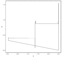
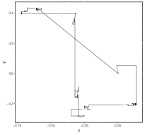
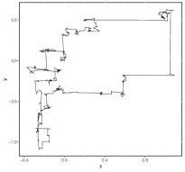
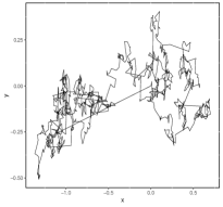
This section will focus on the expressions for the solutions of PDEs involving IFL (3) on the irregular domain in arbitrary dimensions. Although it is difficult to find the Green function Q~rsubscript~𝑄𝑟\widetilde{Q}_{r} and Poisson kernel Prsubscript𝑃𝑟P_{r} on the irregular domain ΩΩ\Omega, the fractional Poisson equation on the irregular domain can be approximated by the whole motion path with a sequence of small ball. According to (5), we know that the solution of (3) on any irregular domain can be simulated via an α𝛼\alpha-stable process (cf. Fig. 1), and this process stops when it reaches the outside of the region. Recall that the solution of (3) corresponds to α𝛼\alpha-stable process Xtαsubscriptsuperscript𝑋𝛼𝑡X^{\alpha}_{t} and can be rewritten in the form of path integral as (cf. [24])

u(𝒙)=𝔼X0α=𝒙[0τΩf(Xsα)ds]+𝔼X0α=𝒙[g(XτΩα)],𝒙Ω,formulae-sequence𝑢𝒙subscript𝔼superscriptsubscript𝑋0𝛼𝒙delimited-[]superscriptsubscript0subscript𝜏Ω𝑓subscriptsuperscript𝑋𝛼𝑠differential-d𝑠subscript𝔼superscriptsubscript𝑋0𝛼𝒙delimited-[]𝑔subscriptsuperscript𝑋𝛼subscript𝜏Ω𝒙Ωu(\bm{x})=\mathbb{E}_{X_{0}^{\alpha}=\bm{x}}\Big{[}\int_{0}^{\tau_{\Omega}}f(X^{\alpha}_{s})\,{\rm d}s\Big{]}+\mathbb{E}_{X_{0}^{\alpha}=\bm{x}}\big{[}g(X^{\alpha}_{\tau_{\Omega}})\big{]},\;\;\bm{x}\in\Omega,

where τΩsubscript𝜏Ω\tau_{\Omega} is the first passage time and XτΩαsubscriptsuperscript𝑋𝛼subscript𝜏ΩX^{\alpha}_{\tau_{\Omega}} is the first passage location on the region nΩsuperscript𝑛Ω\mathbb{R}^{n}\setminus\Omega, and 𝔼𝒙[τΩ]<subscript𝔼𝒙delimited-[]subscript𝜏Ω\mathbb{E}_{\bm{x}}[\tau_{\Omega}]<\infty, for all 𝒙Ω𝒙Ω\bm{x}\in\Omega.

Refer to caption
(a) α=0.4𝛼0.4\alpha=0.4
Refer to caption
(b) α=0.8𝛼0.8\alpha=0.8
Refer to caption
(c) α=1.2𝛼1.2\alpha=1.2
Refer to caption
(d) α=1.6𝛼1.6\alpha=1.6
Figure 1: The motion trajectory of α𝛼\alpha-stable process.
Refer to caption
Refer to caption
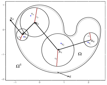
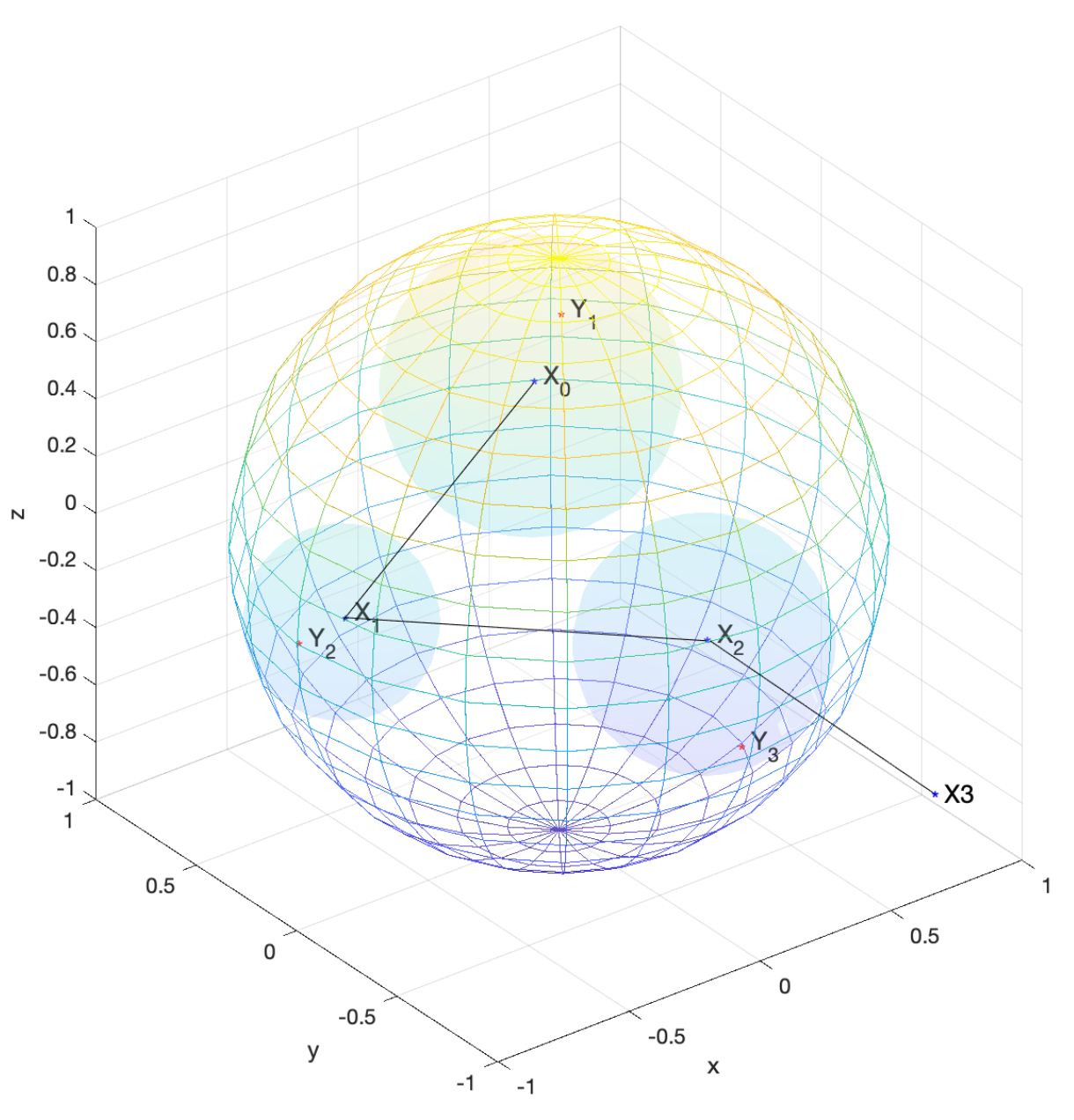
Figure 2: The path of walk; Left: on 222-D irregular domain; Right: on the unit ball in 333-D.

Since the Markov process will leave the given domain at a finite time, the discrete point sequence can reach outside the domain ΩΩ\Omega after a limited number of steps. Therefore, at each jump, the probability of this point leaving the given region at the next move always be positive, that is, P(m<)=1,𝑃superscript𝑚1P(m^{\ast}<\infty)=1, where we denoted by

(17) m=inf{m:XmΩ},superscript𝑚infconditional-set𝑚subscript𝑋𝑚Ωm^{\ast}=\text{inf}\{m:X_{m}\notin\Omega\},

the stopping step for the random walk. Hence, the Monte Carlo method can be use to calculate the existing observation paths, to obtain the value of u(𝒙)𝑢𝒙u(\bm{x}), see Fig. 2.

Theorem 2.6.

Let α(0,2]𝛼02\alpha\in(0,2] and ΩΩ\Omega be an open bounded domain, and assume that fLα1(Ω)C(Ω¯)𝑓subscriptsuperscript𝐿1𝛼Ω𝐶¯Ωf\in L^{1}_{\alpha}(\Omega)\cap C(\overline{\Omega}) and gLα1(nΩ)𝑔subscriptsuperscript𝐿1𝛼superscript𝑛Ωg\in L^{1}_{\alpha}(\mathbb{R}^{n}\!\setminus\!\Omega), then the solution of (3) in Lα1(n)subscriptsuperscript𝐿1𝛼superscript𝑛L^{1}_{\alpha}(\mathbb{R}^{n}) can be expressed as

(18) u(𝒙)=k=1m1ζ(Xk)𝔼Q~rk[f(Yk)]+𝔼Prm1[g(Zm)],Yk𝔹rk,Zkn𝔹rkn,formulae-sequence𝑢𝒙superscriptsubscript𝑘1superscript𝑚1𝜁subscript𝑋𝑘subscript𝔼subscript~𝑄subscript𝑟𝑘delimited-[]𝑓subscript𝑌𝑘subscript𝔼subscript𝑃subscript𝑟superscript𝑚1delimited-[]𝑔subscript𝑍superscript𝑚formulae-sequencesubscript𝑌𝑘subscript𝔹subscript𝑟𝑘subscript𝑍𝑘superscript𝑛subscriptsuperscript𝔹𝑛subscript𝑟𝑘\begin{split}&u(\bm{x})=\sum_{k=1}^{m^{\ast}-1}\zeta(X_{k})\mathbb{E}_{\tilde{Q}_{r_{k}}}[f(Y_{k})]+\mathbb{E}_{P_{r_{m^{\ast}-1}}}[g(Z_{m^{\ast}})],\;\;\;Y_{k}\in\mathbb{B}_{r_{k}},\;Z_{k}\in\mathbb{R}^{n}\!\setminus\!\mathbb{B}^{n}_{r_{k}},\end{split}

where ζ(Xk)𝜁subscript𝑋𝑘\zeta(X_{k}) is the weight function in k𝑘k-th ball,

(19) ζ(Xk)=𝔹rknQrk(Xk,𝒚)d𝒚.𝜁subscript𝑋𝑘subscriptsuperscriptsubscript𝔹subscript𝑟𝑘𝑛subscript𝑄subscript𝑟𝑘subscript𝑋𝑘𝒚differential-d𝒚\zeta(X_{k})=\int_{\mathbb{B}_{r_{k}}^{n}}Q_{r_{k}}(X_{k},\bm{y})\,\mathrm{d}\bm{y}.

In the above, the first expectation represents the contribution of source f𝑓f in k𝑘k-th inside ball associated with the Green’s function Qrksubscript𝑄subscript𝑟𝑘Q_{r_{k}}, and the second one describes a mean value of g𝑔g outside the last ball 𝔹rm1nsubscriptsuperscript𝔹𝑛subscript𝑟superscript𝑚1\mathbb{B}^{n}_{r_{m^{\ast}-1}} associated with Prm1subscript𝑃subscript𝑟superscript𝑚1P_{r_{m^{\ast}-1}}.

Proof 2.7.

The α𝛼\alpha-stable process Xtαsuperscriptsubscript𝑋𝑡𝛼X_{t}^{\alpha} can be surrounded by a series of small balls tangent to region ΩΩ\Omega, that is, we can split the process Xtαsuperscriptsubscript𝑋𝑡𝛼X_{t}^{\alpha} according to the time of movement within the region ΩΩ\Omega. Let 0=τ0<τ1<τ2<<τm=τΩ0subscript𝜏0subscript𝜏1subscript𝜏2subscript𝜏superscript𝑚subscript𝜏Ω0=\tau_{0}<\tau_{1}<\tau_{2}<\cdots<\tau_{m^{\ast}}=\tau_{\Omega}, τksubscript𝜏𝑘\tau_{k} (0<k<m)0𝑘subscript𝑚(0<k<m_{\ast}) denotes the time of movement away from the k𝑘k-th ball. In view of (5), the solution of (3) have the following form

u(𝒙)=𝔼X0α=𝒙[0τΩf(Xsα)ds]+𝔼X0α=x[g(XτΩα)]=𝔼X0α=𝒙[τ0τ1f(Xsα)ds+τ1τ2f(Xsα)ds++τm1τmf(Xsα)ds]+𝔼X0α=𝒙[g(XτΩα)]=𝔼X0α=𝒙[k=0m1τkτk+1f(Xsα)ds]+𝔼X0α=𝒙[g(Xτmα)].𝑢𝒙subscript𝔼superscriptsubscript𝑋0𝛼𝒙delimited-[]superscriptsubscript0subscript𝜏Ω𝑓subscriptsuperscript𝑋𝛼𝑠differential-d𝑠subscript𝔼superscriptsubscript𝑋0𝛼𝑥delimited-[]𝑔subscriptsuperscript𝑋𝛼subscript𝜏Ωsubscript𝔼superscriptsubscript𝑋0𝛼𝒙delimited-[]superscriptsubscriptsubscript𝜏0subscript𝜏1𝑓subscriptsuperscript𝑋𝛼𝑠differential-d𝑠superscriptsubscriptsubscript𝜏1subscript𝜏2𝑓subscriptsuperscript𝑋𝛼𝑠differential-d𝑠superscriptsubscriptsubscript𝜏superscript𝑚1subscript𝜏superscript𝑚𝑓subscriptsuperscript𝑋𝛼𝑠differential-d𝑠subscript𝔼superscriptsubscript𝑋0𝛼𝒙delimited-[]𝑔subscriptsuperscript𝑋𝛼subscript𝜏Ωsubscript𝔼superscriptsubscript𝑋0𝛼𝒙delimited-[]superscriptsubscript𝑘0superscript𝑚1superscriptsubscriptsubscript𝜏𝑘subscript𝜏𝑘1𝑓subscriptsuperscript𝑋𝛼𝑠differential-d𝑠subscript𝔼superscriptsubscript𝑋0𝛼𝒙delimited-[]𝑔subscriptsuperscript𝑋𝛼subscript𝜏superscript𝑚\begin{split}u(\bm{x})&=\mathbb{E}_{X_{0}^{\alpha}=\bm{x}}\Big{[}\int_{0}^{\tau_{\Omega}}f(X^{\alpha}_{s})\,{\rm d}s\Big{]}+\mathbb{E}_{X_{0}^{\alpha}=x}\big{[}g(X^{\alpha}_{\tau_{\Omega}})\big{]}\\ &=\mathbb{E}_{X_{0}^{\alpha}=\bm{x}}\Big{[}\int_{\tau_{0}}^{\tau_{1}}f(X^{\alpha}_{s})\,{\rm d}s+\int_{\tau_{1}}^{\tau_{2}}f(X^{\alpha}_{s})\,{\rm d}s+\cdots+\int_{\tau_{m^{\ast}-1}}^{\tau_{m^{\ast}}}f(X^{\alpha}_{s})\,{\rm d}s\Big{]}+\mathbb{E}_{X_{0}^{\alpha}=\bm{x}}\big{[}g(X^{\alpha}_{\tau_{\Omega}})\big{]}\\ &=\mathbb{E}_{X_{0}^{\alpha}=\bm{x}}\Big{[}\sum_{k=0}^{m^{\ast}-1}\int_{\tau_{k}}^{\tau_{k+1}}f(X^{\alpha}_{s})\,{\rm d}s\Big{]}+\mathbb{E}_{X_{0}^{\alpha}=\bm{x}}\big{[}g(X^{\alpha}_{\tau_{m^{\ast}}})\big{]}.\end{split}

As a result, a similar procedure as in Lemma 2.3 can be applied to each step of the above process. It is clear that each expectation, i.e., 𝔼X0α=𝐱,Xτkα=Xk[τkτk+1f(Xsα)ds]subscript𝔼formulae-sequencesuperscriptsubscript𝑋0𝛼𝐱superscriptsubscript𝑋subscript𝜏𝑘𝛼subscript𝑋𝑘delimited-[]superscriptsubscriptsubscript𝜏𝑘subscript𝜏𝑘1𝑓subscriptsuperscript𝑋𝛼𝑠differential-d𝑠\mathbb{E}_{X_{0}^{\alpha}=\bm{x},X_{\tau_{k}}^{\alpha}=X_{k}}\Big{[}\int_{\tau_{k}}^{\tau_{k+1}}f(X^{\alpha}_{s})\,{\rm d}s\Big{]} can be view as the stochastic solution of the following fractional PDEs with homogeneous boundary condition

{(Δ)α2u(𝒙)=f(𝒙),in𝔹rkn,u(𝒙)=0,onn\𝔹rkn.casessuperscriptΔ𝛼2𝑢𝒙𝑓𝒙insubscriptsuperscript𝔹𝑛subscript𝑟𝑘𝑢𝒙0\onsuperscript𝑛subscriptsuperscript𝔹𝑛subscript𝑟𝑘\begin{cases}(-\Delta)^{\frac{\alpha}{2}}u(\bm{x})=f(\bm{x}),\;&{\rm in}\ \mathbb{B}^{n}_{r_{k}},\\[4.0pt] u(\bm{x})=0,\quad&{\rm on}\ \mathbb{R}^{n}\backslash\mathbb{B}^{n}_{r_{k}}.\end{cases}

Moreover, in the last step, the term 𝔼X0α=𝐱,Xτm1α=Xm1[τm1τmf(Xsα)ds]+𝔼X0α=𝐱[g(Xτmα)]subscript𝔼formulae-sequencesuperscriptsubscript𝑋0𝛼𝐱subscriptsuperscript𝑋𝛼subscript𝜏subscript𝑚1subscript𝑋subscript𝑚1delimited-[]superscriptsubscriptsubscript𝜏subscript𝑚1subscript𝜏subscript𝑚𝑓subscriptsuperscript𝑋𝛼𝑠differential-d𝑠subscript𝔼superscriptsubscript𝑋0𝛼𝐱delimited-[]𝑔subscriptsuperscript𝑋𝛼subscript𝜏subscript𝑚\mathbb{E}_{X_{0}^{\alpha}=\bm{x},{X^{\alpha}_{\tau_{m_{\ast}-1}}}=X_{m_{\ast}-1}}\Big{[}\int_{\tau_{m_{\ast}-1}}^{\tau_{m_{\ast}}}f(X^{\alpha}_{s})\,{\rm d}s\Big{]}+\mathbb{E}_{X_{0}^{\alpha}=\bm{x}}\big{[}g(X^{\alpha}_{\tau_{m_{\ast}}})\big{]} represents the stochastic solution of the following problem

{(Δ)α2u(𝒙)=f(𝒙),in𝔹rm1n,u(𝒙)=g(𝒙),onn\𝔹rm1n.casessuperscriptΔ𝛼2𝑢𝒙𝑓𝒙insubscriptsuperscript𝔹𝑛subscript𝑟subscript𝑚1𝑢𝒙𝑔𝒙\onsuperscript𝑛subscriptsuperscript𝔹𝑛subscript𝑟subscript𝑚1\begin{cases}(-\Delta)^{\frac{\alpha}{2}}u(\bm{x})=f(\bm{x}),\;&{\rm in}\ \mathbb{B}^{n}_{r_{m_{\ast}-1}},\\[4.0pt] u(\bm{x})=g(\bm{x}),\quad&{\rm on}\ \mathbb{R}^{n}\backslash\mathbb{B}^{n}_{r_{m_{\ast}-1}}.\end{cases}

Then, we derive from (2.1) and (12) that

𝔼X0α=𝒙[τkτk+1f(Xsα)ds]=𝔹rknf(𝒚)Qrk(Xk,𝒚)d𝒚=ζ(Xk)𝔹rknf(𝒚)Q~rk(Xk,𝒚)d𝒚=ζ(Xk)𝔼Q~rk[f(Yk)].subscript𝔼superscriptsubscript𝑋0𝛼𝒙delimited-[]superscriptsubscriptsubscript𝜏𝑘subscript𝜏𝑘1𝑓subscriptsuperscript𝑋𝛼𝑠differential-d𝑠subscriptsubscriptsuperscript𝔹𝑛subscript𝑟𝑘𝑓𝒚subscript𝑄subscript𝑟𝑘subscript𝑋𝑘𝒚differential-d𝒚𝜁subscript𝑋𝑘subscriptsubscriptsuperscript𝔹𝑛subscript𝑟𝑘𝑓𝒚subscript~𝑄subscript𝑟𝑘subscript𝑋𝑘𝒚differential-d𝒚𝜁subscript𝑋𝑘subscript𝔼subscript~𝑄subscript𝑟𝑘delimited-[]𝑓subscript𝑌𝑘\begin{split}\mathbb{E}_{X_{0}^{\alpha}=\bm{x}}\Big{[}\int_{\tau_{k}}^{\tau_{k+1}}f(X^{\alpha}_{s})\,{\rm d}s\Big{]}&=\int_{\mathbb{B}^{n}_{r_{k}}}f(\bm{y})Q_{r_{k}}(X_{k},\bm{y})\,\mathrm{d}\bm{y}=\zeta(X_{k})\int_{\mathbb{B}^{n}_{r_{k}}}f(\bm{y})\tilde{Q}_{r_{k}}(X_{k},\bm{y})\,\mathrm{d}\bm{y}\\ &=\zeta(X_{k})\mathbb{E}_{\tilde{Q}_{r_{k}}}[f(Y_{k})].\end{split}

Since τmsubscript𝜏subscript𝑚\tau_{m_{\ast}} denotes the time for the process Xtαsuperscriptsubscript𝑋𝑡𝛼X_{t}^{\alpha} to leave the (m1)subscript𝑚1(m_{\ast}-1)-th ball, and also leave domain ΩΩ\Omega, then

𝔼X0α=𝒙[g(Xτmα)]=𝔼Prm1[g(Zm)].subscript𝔼superscriptsubscript𝑋0𝛼𝒙delimited-[]𝑔subscriptsuperscript𝑋𝛼subscript𝜏subscript𝑚subscript𝔼subscript𝑃subscript𝑟superscript𝑚1delimited-[]𝑔subscript𝑍superscript𝑚\mathbb{E}_{X_{0}^{\alpha}=\bm{x}}\big{[}g(X^{\alpha}_{\tau_{m_{\ast}}})\big{]}=\mathbb{E}_{P_{r_{m^{\ast}-1}}}[g(Z_{m^{\ast}})].

Consequently, a combination of the above results lead to the desired result.

2.3 Efficient algorithm

This section describe the Monto Carlo method using Green function and the representation (12) and (18) to solve the fractional PDEs on bounded domain. To fix the idea, we only consider the algorithm based on the representation (18), as (12) is a special case of (18).

Instead of simulating the irregular trajectories of symmetric α𝛼\alpha-stable processes, we take advantage of the explicit expressions of Q~rsubscript~𝑄𝑟\widetilde{Q}_{r} and Prsubscript𝑃𝑟P_{r} as the probability density functions, which gives the transition probability of the symmetric α𝛼\alpha-stable process trajectory inside the ball during its passage from the center to the boundary ΩΩ\partial\Omega or outside the domain ΩΩ\Omega (cf. Fig. 2). More precisely, the representation (18) allows us to construct a sequence of inside balls {𝔹rin:=𝔹rin,𝒙i}i0subscriptassignsubscriptsuperscript𝔹𝑛subscript𝑟𝑖subscriptsuperscript𝔹𝑛subscript𝒙𝑖subscript𝑟𝑖𝑖0\{\mathbb{B}^{n}_{r_{i}}:=\mathbb{B}^{n,\bm{x}_{i}}_{r_{i}}\}_{i\geq 0} tangent to the boundary ΩΩ\partial\Omega. In each ball, we construct a random variable whose value is only obtained inside the corresponding ball. The expected value of the symmetric α𝛼\alpha-stable process integral is replaced by the weighted expected value of this set of random variables. The centers of these balls are generated by a series of discrete transitions in continuous space nsuperscript𝑛\mathbb{R}^{n} that eventually terminate when they first reach the outside of domain ΩΩ\Omega.

We denote by Xisubscript𝑋𝑖X_{i} the i𝑖i-th random variable, and then generate the corresponding inside ball centered at Xisubscript𝑋𝑖X_{i} tangent the boundary ΩΩ\partial\Omega, i.e., 𝔹rin,Xisubscriptsuperscript𝔹𝑛subscript𝑋𝑖subscript𝑟𝑖\mathbb{B}^{n,X_{i}}_{r_{i}}. It is evident that the closer Xisubscript𝑋𝑖X_{i} approaches to the center of ΩΩ\Omega, the bigger area of the ball will be. In other words, the area Ω𝔹rin,XiΩsubscriptsuperscript𝔹𝑛subscript𝑋𝑖subscript𝑟𝑖\Omega\setminus\mathbb{B}^{n,X_{i}}_{r_{i}} will decrease as it moves away from the center. One verifies readily that the next time the ball moves, the less likely it is to be in Ω𝔹rin,XiΩsubscriptsuperscript𝔹𝑛subscript𝑋𝑖subscript𝑟𝑖\Omega\setminus\mathbb{B}^{n,X_{i}}_{r_{i}}. Conversely, when the center of the current ball is near ΩΩ\partial\Omega, the probability that the ball will be in Ω𝔹rin,XiΩsubscriptsuperscript𝔹𝑛subscript𝑋𝑖subscript𝑟𝑖\Omega\setminus\mathbb{B}^{n,X_{i}}_{r_{i}} on its next move increases. Given an accuracy threshold ε>0𝜀0\varepsilon>0, we define an inwardly ‘thickening’ the boundary ΩΩ\partial\Omega as (see Fig. 2 (left)):

(20) Γε={𝒙Ω:dist(𝒙,Ω)<ε},subscriptΓ𝜀conditional-set𝒙Ωdist𝒙Ω𝜀\Gamma_{\varepsilon}=\{\bm{x}\in\Omega:{\rm dist}(\bm{x},\partial\Omega)<\varepsilon\},

where dist(𝒙,Ω)dist𝒙Ω{\rm dist}(\bm{x},\partial\Omega) denotes the distance from 𝒙Ω𝒙Ω\bm{x}\in\Omega to ΩΩ\partial\Omega. Therefore, to reduce the calculation, we assume that the Moto Carlo process stops when it reaches ΓεΩcsubscriptΓ𝜀superscriptΩ𝑐\Gamma_{\varepsilon}\cup\Omega^{c}. When ε𝜀\varepsilon is small enough if the ball moves into this domain ΓεsubscriptΓ𝜀\Gamma_{\varepsilon}, it’s considered outside the domain ΩΩ\Omega.

Therefore, in each experiment, we need to simulate several important quantities as below

(i). The coordinates of the center of i𝑖i-th ball;

(ii). The radius of the ball risubscript𝑟𝑖r_{i}, which is the distance in each discrete jump;

(iii). The weight of the expectation ζ(𝒙i)𝜁subscript𝒙𝑖\zeta(\bm{x}_{i}) ;

(iv). The expectation of the random variable in each ball 𝔼[f(Y)]𝔼delimited-[]𝑓𝑌\mathbb{E}[f(Y)].

Dealing with the above quantities in high dimensional Cartesian coordinates appears difficult, therefore, to simplify the implementation, we recommend proceeding with this calculation in spherical coordinates. To this end, we denoted by 𝒙^=𝒙/|𝒙|^𝒙𝒙𝒙\hat{\bm{x}}=\bm{x}/|\bm{x}| the unit vector along the nonzero vector 𝒙𝒙\bm{x}. We now recall the d𝑑d-dimensional spherical coordinates

(21) x1=ρcosθ1;x2=ρsinθ1cosθ2;;xn1=ρsinθ1sinθn2cosθn1;xn=ρsinθ1sinθn2sinθn1,θ1,,θn2[0,π],θn1[0,2π],formulae-sequencesubscript𝑥1𝜌subscript𝜃1formulae-sequencesubscript𝑥2𝜌subscript𝜃1subscript𝜃2formulae-sequencesubscript𝑥𝑛1𝜌subscript𝜃1subscript𝜃𝑛2subscript𝜃𝑛1formulae-sequencesubscript𝑥𝑛𝜌subscript𝜃1subscript𝜃𝑛2subscript𝜃𝑛1subscript𝜃1formulae-sequencesubscript𝜃𝑛20𝜋subscript𝜃𝑛102𝜋\begin{split}&x_{1}=\rho\cos\theta_{1};\;x_{2}=\rho\sin\theta_{1}\cos\theta_{2};\;\cdots\cdots;\;x_{n-1}=\rho\sin\theta_{1}\cdots\sin\theta_{n-2}\cos\theta_{n-1};\\ &x_{n}=\rho\sin\theta_{1}\cdots\sin\theta_{n-2}\sin\theta_{n-1},\;\;\;\theta_{1},\cdots,\theta_{n-2}\in[0,\pi],\;\;\theta_{n-1}\in[0,2\pi],\end{split}

with the spherical volume element

(22) d𝒙=ρn1sinn2θ1sinn3θ2sinθn2dρdθ1dθ2dθn1.d𝒙superscript𝜌𝑛1superscript𝑛2subscript𝜃1superscript𝑛3subscript𝜃2subscript𝜃𝑛2d𝜌dsubscript𝜃1dsubscript𝜃2dsubscript𝜃𝑛1\begin{split}\mathrm{d}\bm{x}=\rho^{n-1}\sin^{n-2}\theta_{1}\sin^{n-3}\theta_{2}\cdots\sin\theta_{n-2}\,\mathrm{d}\rho\,\mathrm{d}\theta_{1}\,\mathrm{d}\theta_{2}\cdots\mathrm{d}\theta_{n-1}.\end{split}

2.3.1 Computation of the jump distance and weight function ζ(x)𝜁𝑥\zeta(x)

We can evaluate the jump distance (denoted by γ𝛾\gamma) from the current ball to the next ball by using the following formula, which indicates the jump distance is a uniformly distributed random number.

Lemma 2.8.

Let α(0,2]𝛼02\alpha\in(0,2] and let the radius of the current ball r>0𝑟0r>0. Assume that the ball jumps in the region ΩΩ\Omega, then the jump distance γ𝛾\gamma from the current ball to the next ball is given by

(23) γ(ω;r,n,α)=r2B(1α2,α2)B1(πωsin(πα/2);1α2,α2),ω(0,1),formulae-sequence𝛾𝜔𝑟𝑛𝛼superscript𝑟2𝐵1𝛼2𝛼2superscript𝐵1𝜋𝜔𝜋𝛼21𝛼2𝛼2𝜔01\displaystyle\gamma(\omega;r,n,\alpha)=\sqrt{\frac{r^{2}}{B(1-\frac{\alpha}{2},\frac{\alpha}{2})-B^{-1}(\frac{\pi\,\omega}{\sin(\pi\alpha/2)};1-\frac{\alpha}{2},\frac{\alpha}{2})}},\;\;\;\omega\in(0,1),

where B1(;a,b)superscript𝐵1𝑎𝑏B^{-1}(\cdot\,;a,b) denote the inverse function of incomplete Beta function B(;a,b)𝐵𝑎𝑏B(\cdot\,;a,b), and B(a,b):=B(1;a,b)assign𝐵𝑎𝑏𝐵1𝑎𝑏B(a,b):=B(1;a,b) denote the Beta function.

Proof 2.9.

Let 𝐱=|𝐱|en𝐱𝐱subscript𝑒𝑛\bm{x}=|\bm{x}|e_{n}, then we have |𝐱𝐳|2=|𝐱|2+|𝐳|22|𝐱||𝐳|cosθ=ρ2+|𝐱|22|𝐱|ρcosθsuperscript𝐱𝐳2superscript𝐱2superscript𝐳22𝐱𝐳𝜃superscript𝜌2superscript𝐱22𝐱𝜌𝜃|\bm{x}-\bm{z}|^{2}=|\bm{x}|^{2}+|\bm{z}|^{2}-2|\bm{x}||\bm{z}|\cos\theta=\rho^{2}+|\bm{x}|^{2}-2|\bm{x}|\rho\cos\theta (see Fig. 3). For |𝐳|>r𝐳𝑟|\bm{z}|>r and 𝐱𝟎𝐱0\bm{x}\neq\bm{0}, we find from (8) and the above identity that

r<|𝒛|<γPr(𝒙,𝒛)d𝒛subscript𝑟𝒛𝛾subscript𝑃𝑟𝒙𝒛differential-d𝒛\displaystyle\int_{r<|\bm{z}|<\gamma}P_{r}(\bm{x},\bm{z})\,\mathrm{d}\bm{z}
(24) =2πC~nα(r2|𝒙|2)α2k=1n30πsinkθdθrγ0πρn1sinn2θ(ρ2r2)α/2(ρ2+|𝒙|22ρ|𝒙|cosθ)n/2dθdρabsent2𝜋subscriptsuperscript~𝐶𝛼𝑛superscriptsuperscript𝑟2superscript𝒙2𝛼2superscriptsubscriptproduct𝑘1𝑛3superscriptsubscript0𝜋superscript𝑘𝜃d𝜃superscriptsubscript𝑟𝛾superscriptsubscript0𝜋superscript𝜌𝑛1superscript𝑛2𝜃superscriptsuperscript𝜌2superscript𝑟2𝛼2superscriptsuperscript𝜌2superscript𝒙22𝜌𝒙𝜃𝑛2differential-d𝜃differential-d𝜌\displaystyle\quad\quad\quad=2\pi\widetilde{C}^{\alpha}_{n}(r^{2}-|\bm{x}|^{2})^{\frac{\alpha}{2}}\prod_{k=1}^{n-3}\int_{0}^{\pi}\sin^{k}\theta\mathrm{d}\theta\int_{r}^{\gamma}\!\int_{0}^{\pi}\frac{\rho^{n-1}\sin^{n-2}\theta}{(\rho^{2}-r^{2})^{\alpha/2}(\rho^{2}+|\bm{x}|^{2}-2\rho|\bm{x}|\cos\theta)^{n/2}}\mathrm{d}\theta\mathrm{d}\rho
=2πC~nα(r¯21)α2k=1n30πsinkθdθrγρ¯n1(ρ¯2r2)α/2λ(ρ¯)dρ¯,absent2𝜋subscriptsuperscript~𝐶𝛼𝑛superscriptsuperscript¯𝑟21𝛼2superscriptsubscriptproduct𝑘1𝑛3superscriptsubscript0𝜋superscript𝑘𝜃d𝜃superscriptsubscript𝑟𝛾superscript¯𝜌𝑛1superscriptsuperscript¯𝜌2superscript𝑟2𝛼2𝜆¯𝜌differential-d¯𝜌\displaystyle\quad\quad\quad=2\pi\widetilde{C}^{\alpha}_{n}(\bar{r}^{2}-1)^{\frac{\alpha}{2}}\prod_{k=1}^{n-3}\int_{0}^{\pi}\sin^{k}\theta\mathrm{d}\theta\int_{r}^{\gamma}\!\frac{\bar{\rho}^{n-1}}{(\bar{\rho}^{2}-r^{2})^{\alpha/2}}\lambda(\bar{\rho})\,\mathrm{d}\bar{\rho},

where we used r¯=r/|𝐱|>1¯𝑟𝑟𝐱1\bar{r}=r/|\bm{x}|>1, ρ¯=ρ/|𝐱|>1¯𝜌𝜌𝐱1\bar{\rho}=\rho/|\bm{x}|>1 in the last identity, and denoted

λ(ρ¯)=0πsinn2θ(ρ¯2+12ρ¯cosθ)n/2dθ.𝜆¯𝜌superscriptsubscript0𝜋superscript𝑛2𝜃superscriptsuperscript¯𝜌212¯𝜌𝜃𝑛2differential-d𝜃\lambda(\bar{\rho})=\int_{0}^{\pi}\frac{\sin^{n-2}\theta}{(\bar{\rho}^{2}+1-2\bar{\rho}\cos\theta)^{n/2}}\,\mathrm{d}\theta.

According to [8, (A.25)], we have

(25) λ(ρ¯)=1ρ¯n2(ρ¯21)0πsinn2σdσ.𝜆¯𝜌1superscript¯𝜌𝑛2superscript¯𝜌21superscriptsubscript0𝜋superscript𝑛2𝜎d𝜎\lambda(\bar{\rho})=\frac{1}{\bar{\rho}^{n-2}(\bar{\rho}^{2}-1)}\int_{0}^{\pi}\sin^{n-2}\sigma\,\mathrm{d}\sigma.

Then, we derive from (2.9) and (25) that

(26) r<|𝒛|<γPr(𝒙,𝒛)d𝒛=2πC~nα(r¯21)α/2k=1n20πsinkθdθrγρ¯(ρ¯2r¯2)α/2(ρ¯21)dρ¯.subscript𝑟𝒛𝛾subscript𝑃𝑟𝒙𝒛differential-d𝒛2𝜋subscriptsuperscript~𝐶𝛼𝑛superscriptsuperscript¯𝑟21𝛼2superscriptsubscriptproduct𝑘1𝑛2superscriptsubscript0𝜋superscript𝑘𝜃d𝜃superscriptsubscript𝑟𝛾¯𝜌superscriptsuperscript¯𝜌2superscript¯𝑟2𝛼2superscript¯𝜌21differential-d¯𝜌\int_{r<|\bm{z}|<\gamma}P_{r}(\bm{x},\bm{z})\,\mathrm{d}\bm{z}=2\pi\widetilde{C}^{\alpha}_{n}(\bar{r}^{2}-1)^{\alpha/2}\prod_{k=1}^{n-2}\int_{0}^{\pi}\sin^{k}\theta\,\mathrm{d}\theta\int_{r}^{\gamma}\frac{\bar{\rho}}{(\bar{\rho}^{2}-\bar{r}^{2})^{\alpha/2}(\bar{\rho}^{2}-1)}\,\mathrm{d}\bar{\rho}.

Recall the formulas [8, Proposition A.10],

(27) πk=1n20πsinkθdθ=πn/2Γ(n/2).𝜋superscriptsubscriptproduct𝑘1𝑛2superscriptsubscript0𝜋superscript𝑘𝜃d𝜃superscript𝜋𝑛2Γ𝑛2\pi\prod_{k=1}^{n-2}\int_{0}^{\pi}\sin^{k}\theta\,\mathrm{d}\theta=\frac{\pi^{n/2}}{\Gamma(n/2)}.

In view of (26) and (27), we make the change of variable t=(ρ¯/r¯)21𝑡superscript¯𝜌¯𝑟21t=(\bar{\rho}/\bar{r})^{2}-1, and obtain

(28) r<|𝒛|<γPr(𝒙,𝒛)d𝒛=πn/2Γ(n/2)C~nα0γ2r211(1+t)tα/2dt,subscript𝑟𝒛𝛾subscript𝑃𝑟𝒙𝒛differential-d𝒛superscript𝜋𝑛2Γ𝑛2subscriptsuperscript~𝐶𝛼𝑛superscriptsubscript0superscript𝛾2superscript𝑟2111𝑡superscript𝑡𝛼2differential-d𝑡\begin{split}\int_{r<|\bm{z}|<\gamma}P_{r}(\bm{x},\bm{z})\,\mathrm{d}\bm{z}&=\frac{\pi^{n/2}}{\Gamma(n/2)}\widetilde{C}^{\alpha}_{n}\int_{0}^{\frac{\gamma^{2}}{r^{2}}-1}\frac{1}{(1+t)t^{\alpha/2}}\,\mathrm{d}t,\end{split}

let t~=1/(1+t)~𝑡11𝑡\tilde{t}=1/(1+t), then we have

(29) r<|𝒛|<γPr(𝒙,𝒛)d𝒛=πn/2Γ(n/2)C~nαr2γ21t~α/2(1t~)α/21dt~.subscript𝑟𝒛𝛾subscript𝑃𝑟𝒙𝒛differential-d𝒛superscript𝜋𝑛2Γ𝑛2subscriptsuperscript~𝐶𝛼𝑛superscriptsubscriptsuperscript𝑟2superscript𝛾21superscript~𝑡𝛼2superscript1~𝑡𝛼21differential-d~𝑡\begin{split}\int_{r<|\bm{z}|<\gamma}P_{r}(\bm{x},\bm{z})\,\mathrm{d}\bm{z}&=\frac{\pi^{n/2}}{\Gamma(n/2)}\widetilde{C}^{\alpha}_{n}\int_{\frac{r^{2}}{\gamma^{2}}}^{1}\tilde{t}^{-\alpha/2}(1-\tilde{t})^{\alpha/2-1}\,\mathrm{d}\tilde{t}.\end{split}

Thanks to Prsubscript𝑃𝑟P_{r} is a probability density function (cf. (15)), then

(30) r<|𝒛|<γPr(𝒙,𝒛)d𝒛=πn/2Γ(n/2)C~nα[B(1α2,α2)B(r2γ2;1α2,α2)]:=ω(0,1).subscript𝑟𝒛𝛾subscript𝑃𝑟𝒙𝒛differential-d𝒛superscript𝜋𝑛2Γ𝑛2subscriptsuperscript~𝐶𝛼𝑛delimited-[]𝐵1𝛼2𝛼2𝐵superscript𝑟2superscript𝛾21𝛼2𝛼2assign𝜔01\int_{r<|\bm{z}|<\gamma}P_{r}(\bm{x},\bm{z})\,\mathrm{d}\bm{z}=\frac{\pi^{n/2}}{\Gamma(n/2)}\widetilde{C}^{\alpha}_{n}\Big{[}B(1-\frac{\alpha}{2},\frac{\alpha}{2})-B\Big{(}\frac{r^{2}}{\gamma^{2}};1-\frac{\alpha}{2},\frac{\alpha}{2}\Big{)}\Big{]}:=\omega\in(0,1).

Moreover, by the inverse of the distribution function and (11), we can easily obtain the desired result (23).

n1superscript𝑛1{\color[rgb]{0,0,0}\definecolor[named]{pgfstrokecolor}{rgb}{0,0,0}\pgfsys@color@gray@stroke{0}\pgfsys@color@gray@fill{0}\mathbb{R}^{n-1}}ensubscript𝑒𝑛{\color[rgb]{0,0,0}\definecolor[named]{pgfstrokecolor}{rgb}{0,0,0}\pgfsys@color@gray@stroke{0}\pgfsys@color@gray@fill{0}e_{n}}θ𝜃\thetaXsuperscript𝑋X^{\ast}Ysuperscript𝑌Y^{\ast}
Figure 3: The diagram of coordinate axes after rotation

We reformulate Green’s function into a concise form, which helps us evaluate the weight function ζ(𝒙)𝜁𝒙\zeta(\bm{x}) of each ball more easily. In the following Lemma, we use r=ri𝑟subscript𝑟𝑖r=r_{i} for simplicity.

Lemma 2.10.

For r>0𝑟0r>0, ζ(𝐱)𝜁𝐱\zeta(\bm{x}) in Lemma 2.3 can be computed by

(31) ζ(𝒙)=C^nα𝔹rn|𝒚𝒙|αn[B(nα2,α2)B(ϱ(𝒙,𝒚);nα2,α2)]d𝒚.𝜁𝒙subscriptsuperscript^𝐶𝛼𝑛subscriptsubscriptsuperscript𝔹𝑛𝑟superscript𝒚𝒙𝛼𝑛delimited-[]𝐵𝑛𝛼2𝛼2𝐵superscriptitalic-ϱ𝒙𝒚𝑛𝛼2𝛼2differential-d𝒚\begin{split}\zeta(\bm{x})=\widehat{C}^{\alpha}_{n}\displaystyle\int_{\mathbb{B}^{n}_{r}}|\bm{y}-\bm{x}|^{\alpha-n}\Big{[}B\Big{(}\frac{n-\alpha}{2},\frac{\alpha}{2}\Big{)}-B\Big{(}\varrho^{\ast}(\bm{x},\bm{y});\frac{n-\alpha}{2},\frac{\alpha}{2}\Big{)}\Big{]}\,\mathrm{d}\bm{y}.\end{split}

In particular, if 𝐱=𝟎𝐱0\bm{x}=\bm{0}, we have

(32) ζ(𝟎)=rα2α1Γ2(α2)01ρ~α1[B(nα2,α2)B(ρ~2;nα2,α2)]dρ~.𝜁0superscript𝑟𝛼superscript2𝛼1superscriptΓ2𝛼2superscriptsubscript01superscript~𝜌𝛼1delimited-[]𝐵𝑛𝛼2𝛼2𝐵superscript~𝜌2𝑛𝛼2𝛼2differential-d~𝜌\zeta(\bm{0})=\frac{r^{\alpha}}{2^{\alpha-1}\Gamma^{2}(\frac{\alpha}{2})}\int_{0}^{1}\tilde{\rho}^{\alpha-1}\Big{[}B\Big{(}\frac{n-\alpha}{2},\frac{\alpha}{2}\Big{)}-B\Big{(}\tilde{\rho}^{2};\frac{n-\alpha}{2},\frac{\alpha}{2}\Big{)}\Big{]}\,\mathrm{d}\tilde{\rho}.

Proof 2.11.

In view of (9), we can rewritten the Green’s function as

Qr(𝒙,𝒚)=C^nα|𝒚𝒙|αn0ϱ(𝒙,𝒚)tα/21(1+t)n2dt=C^nα|𝒚𝒙|αnϱ(𝒙,𝒚)1(1m1)α/21(1m)n21m2dm=C^nα|𝒚𝒙|αnϱ(𝒙,𝒚)1mnα21(1m)α/21dm=C^nα|𝒚𝒙|αn[B(nα2,α2)B(ϱ(𝒙,𝒚);nα2,α2)],subscript𝑄𝑟𝒙𝒚subscriptsuperscript^𝐶𝛼𝑛superscript𝒚𝒙𝛼𝑛superscriptsubscript0italic-ϱ𝒙𝒚superscript𝑡𝛼21superscript1𝑡𝑛2differential-d𝑡subscriptsuperscript^𝐶𝛼𝑛superscript𝒚𝒙𝛼𝑛superscriptsubscriptsuperscriptitalic-ϱ𝒙𝒚1superscript1𝑚1𝛼21superscript1𝑚𝑛21superscript𝑚2differential-d𝑚subscriptsuperscript^𝐶𝛼𝑛superscript𝒚𝒙𝛼𝑛superscriptsubscriptsuperscriptitalic-ϱ𝒙𝒚1superscript𝑚𝑛𝛼21superscript1𝑚𝛼21differential-d𝑚subscriptsuperscript^𝐶𝛼𝑛superscript𝒚𝒙𝛼𝑛delimited-[]𝐵𝑛𝛼2𝛼2𝐵superscriptitalic-ϱ𝒙𝒚𝑛𝛼2𝛼2\begin{split}Q_{r}(\bm{x},\bm{y})&=\widehat{C}^{\alpha}_{n}|\bm{y}-\bm{x}|^{\alpha-n}\int_{0}^{\varrho(\bm{x},\bm{y})}\frac{t^{\alpha/2-1}}{(1+t)^{\frac{n}{2}}}\,\mathrm{d}t\\ &=\widehat{C}^{\alpha}_{n}|\bm{y}-\bm{x}|^{\alpha-n}\int_{\varrho^{\ast}(\bm{x},\bm{y})}^{1}\Big{(}\frac{1}{m}-1\Big{)}^{\alpha/2-1}\Big{(}\frac{1}{m}\Big{)}^{-\frac{n}{2}}\frac{1}{m^{2}}\,\mathrm{d}m\\ &=\widehat{C}^{\alpha}_{n}|\bm{y}-\bm{x}|^{\alpha-n}\int_{\varrho^{\ast}(\bm{x},\bm{y})}^{1}m^{\frac{n-\alpha}{2}-1}(1-m)^{\alpha/2-1}\,\mathrm{d}m\\ &=\widehat{C}^{\alpha}_{n}|\bm{y}-\bm{x}|^{\alpha-n}\Big{[}B\Big{(}\frac{n-\alpha}{2},\frac{\alpha}{2}\Big{)}-B\Big{(}\varrho^{\ast}(\bm{x},\bm{y});\frac{n-\alpha}{2},\frac{\alpha}{2}\Big{)}\Big{]},\end{split}

where

ϱ(𝒙,𝒚)=r2|𝒙𝒚|2(r2|𝒙|2)(r2|𝒚|2)+r2|𝒙𝒚|2.superscriptitalic-ϱ𝒙𝒚superscript𝑟2superscript𝒙𝒚2superscript𝑟2superscript𝒙2superscript𝑟2superscript𝒚2superscript𝑟2superscript𝒙𝒚2\begin{split}&\varrho^{\ast}(\bm{x},\bm{y})=\frac{r^{2}|\bm{x}-\bm{y}|^{2}}{(r^{2}-|\bm{x}|^{2})(r^{2}-|\bm{y}|^{2})+r^{2}|\bm{x}-\bm{y}|^{2}}.\end{split}

This together with (13) yields

ζ(𝒙)=C^nα𝔹rn|𝒚𝒙|αn[B(nα2,α2)B(ϱ(𝒙,𝒚);nα2,α2)]d𝒚.𝜁𝒙subscriptsuperscript^𝐶𝛼𝑛subscriptsubscriptsuperscript𝔹𝑛𝑟superscript𝒚𝒙𝛼𝑛delimited-[]𝐵𝑛𝛼2𝛼2𝐵superscriptitalic-ϱ𝒙𝒚𝑛𝛼2𝛼2differential-d𝒚\zeta(\bm{x})=\widehat{C}^{\alpha}_{n}\displaystyle\int_{\mathbb{B}^{n}_{r}}|\bm{y}-\bm{x}|^{\alpha-n}\Big{[}B\Big{(}\frac{n-\alpha}{2},\frac{\alpha}{2}\Big{)}-B\Big{(}\varrho^{\ast}(\bm{x},\bm{y});\frac{n-\alpha}{2},\frac{\alpha}{2}\Big{)}\Big{]}\mathrm{d}\bm{y}.

Moreover, we obtain from (14) that

(33) Q~r(𝒙,𝒚)=C^nα|𝒚𝒙|αn[B(nα2,α2)B(ϱ(𝒙,𝒚);nα2,α2)]ζ(𝒙).subscript~𝑄𝑟𝒙𝒚subscriptsuperscript^𝐶𝛼𝑛superscript𝒚𝒙𝛼𝑛delimited-[]𝐵𝑛𝛼2𝛼2𝐵superscriptitalic-ϱ𝒙𝒚𝑛𝛼2𝛼2𝜁𝒙\widetilde{Q}_{r}(\bm{x},\bm{y})=\frac{\widehat{C}^{\alpha}_{n}|\bm{y}-\bm{x}|^{\alpha-n}[B(\frac{n-\alpha}{2},\frac{\alpha}{2})-B(\varrho^{\ast}(\bm{x},\bm{y});\frac{n-\alpha}{2},\frac{\alpha}{2})]}{\zeta(\bm{x})}.

In particular, if 𝐱=𝟎𝐱0\bm{x}=\bm{0}, we have

ζ(𝟎)=C^nα𝔹rn|𝒚|αn[B(nα2,α2)B(|𝒚|2;nα2,α2)]d𝒚=2πC^nαk=1n20πsinkθdθ0rρα1[B(nα2,α2)B(ρ2;nα2,α2)]dρ=12α1Γ2(α2)0rρα1[B(nα2,α2)B(ρ2;nα2,α2)]dρ,𝜁0subscriptsuperscript^𝐶𝛼𝑛subscriptsubscriptsuperscript𝔹𝑛𝑟superscript𝒚𝛼𝑛delimited-[]𝐵𝑛𝛼2𝛼2𝐵superscript𝒚2𝑛𝛼2𝛼2differential-d𝒚2𝜋subscriptsuperscript^𝐶𝛼𝑛superscriptsubscriptproduct𝑘1𝑛2superscriptsubscript0𝜋superscript𝑘𝜃d𝜃superscriptsubscript0𝑟superscript𝜌𝛼1delimited-[]𝐵𝑛𝛼2𝛼2𝐵superscript𝜌2𝑛𝛼2𝛼2differential-d𝜌1superscript2𝛼1superscriptΓ2𝛼2superscriptsubscript0𝑟superscript𝜌𝛼1delimited-[]𝐵𝑛𝛼2𝛼2𝐵superscript𝜌2𝑛𝛼2𝛼2differential-d𝜌\begin{split}\zeta(\bm{0})&=\widehat{C}^{\alpha}_{n}\displaystyle\int_{\mathbb{B}^{n}_{r}}|\bm{y}|^{\alpha-n}\Big{[}B\Big{(}\frac{n-\alpha}{2},\frac{\alpha}{2}\Big{)}-B\Big{(}|\bm{y}|^{2};\frac{n-\alpha}{2},\frac{\alpha}{2}\Big{)}\Big{]}\,\mathrm{d}\bm{y}\\ &=2\pi\widehat{C}^{\alpha}_{n}\prod_{k=1}^{n-2}\int_{0}^{\pi}\sin^{k}\theta\mathrm{d}\theta\int_{0}^{r}\rho^{\alpha-1}\Big{[}B\Big{(}\frac{n-\alpha}{2},\frac{\alpha}{2}\Big{)}-B\Big{(}\rho^{2};\frac{n-\alpha}{2},\frac{\alpha}{2}\Big{)}\Big{]}\,\mathrm{d}\rho\\ &=\frac{1}{2^{\alpha-1}\Gamma^{2}(\frac{\alpha}{2})}\int_{0}^{r}\rho^{\alpha-1}\Big{[}B\Big{(}\frac{n-\alpha}{2},\frac{\alpha}{2}\Big{)}-B\Big{(}\rho^{2};\frac{n-\alpha}{2},\frac{\alpha}{2}\Big{)}\Big{]}\,\mathrm{d}\rho,\end{split}

We then conclude that the desired result (32) holds under substitution ρ=rρ~𝜌𝑟~𝜌\rho=r\tilde{\rho}. This ends the proof.

Remark 2.12.

It should be pointed out that ζ(𝟎)𝜁0\zeta(\bm{0}) can be accurately computed by Jacobi-Gauss quadrature over the interval (0,1)01(0,1) with index (0,α1)0𝛼1(0,\alpha-1). For convenience, in actual computations we adopt the Monte Carlo integration for the calculation of the integral ζ(𝒙).𝜁𝒙\zeta(\bm{x}).

2.3.2 The Monte Carlo method

In our simulation, the explicit expression of density functions Pr(𝒙,𝒛)subscript𝑃𝑟𝒙𝒛P_{r}(\bm{x},\bm{z}) and Q~(𝒙,𝒚)~𝑄𝒙𝒚\widetilde{Q}(\bm{x},\bm{y}) play an essential role in constructing transition probabilities for a sequence of discrete points outside the ball and the random variables inside the ball, respectively. We now describe the implementations of the Monte Carlo method for the solution of (3). For any given point 𝒙0Ωsubscript𝒙0Ω\bm{x}_{0}\in\Omega, to evaluate u(𝒙0)𝑢subscript𝒙0u(\bm{x}_{0}), we first calculate the shortest distance r1=dist(𝒙0,Γε)subscript𝑟1distsubscript𝒙0subscriptΓ𝜀r_{1}={\rm dist}(\bm{x}_{0},\Gamma_{\varepsilon}) from 𝒙0subscript𝒙0\bm{x}_{0} to the domain ΓεsubscriptΓ𝜀\Gamma_{\varepsilon}, and then draw a inside ball 𝔹r1nsubscriptsuperscript𝔹𝑛subscript𝑟1\mathbb{B}^{n}_{r_{1}} tangent to the domain ΓεsubscriptΓ𝜀\Gamma_{\varepsilon} centered at 𝒙0subscript𝒙0\bm{x}_{0} with radius r1subscript𝑟1r_{1}. Next, we construct a random variable X1subscript𝑋1X_{1} (located at 𝒙1subscript𝒙1\bm{x}_{1}) for outside sphere 𝔹r1nsubscriptsuperscript𝔹𝑛subscript𝑟1\mathbb{B}^{n}_{r_{1}} associated with the corresponding density function Pr1(𝒙0,𝒙1)subscript𝑃subscript𝑟1subscript𝒙0subscript𝒙1P_{r_{1}}(\bm{x}_{0},\bm{x}_{1}), and construct another random variable Y1subscript𝑌1Y_{1} (located at 𝒚1subscript𝒚1\bm{y}_{1}) for inside the ball 𝔹r1nsubscriptsuperscript𝔹𝑛subscript𝑟1\mathbb{B}^{n}_{r_{1}} associated with the density function Q~(𝒙0,𝒚1)~𝑄subscript𝒙0subscript𝒚1\widetilde{Q}(\bm{x}_{0},\bm{y}_{1}).

  • If X1=𝒙1subscript𝑋1subscript𝒙1X_{1}=\bm{x}_{1} is outside the region ΩΩ\Omega, then the value of u(𝒙0)𝑢subscript𝒙0u(\bm{x}_{0}) can be expressed as:

    u(𝒙0)=ζ(𝒙0)𝔼𝒙0[f(Y1)]+𝔼𝒙0[g(X1)].𝑢subscript𝒙0𝜁subscript𝒙0subscript𝔼subscript𝒙0delimited-[]𝑓subscript𝑌1subscript𝔼subscript𝒙0delimited-[]𝑔subscript𝑋1u(\bm{x}_{0})=\zeta(\bm{x}_{0})\mathbb{E}_{\bm{x}_{0}}[f(Y_{1})]+\mathbb{E}_{\bm{x}_{0}}[g(X_{1})].

    If X1=𝒙1subscript𝑋1subscript𝒙1X_{1}=\bm{x}_{1} is inside the region ΩΩ\Omega, we compute the distance r2=dist(𝒙1,Γε)subscript𝑟2distsubscript𝒙1subscriptΓ𝜀r_{2}={\rm dist}(\bm{x}_{1},\Gamma_{\varepsilon}) from x1subscript𝑥1x_{1} to the domain ΓεsubscriptΓ𝜀\Gamma_{\varepsilon}, and draw a new inside ball 𝔹r2nsubscriptsuperscript𝔹𝑛subscript𝑟2\mathbb{B}^{n}_{r_{2}} tangent to the boundary ΓεsubscriptΓ𝜀\Gamma_{\varepsilon} centered at 𝒙1subscript𝒙1\bm{x}_{1} with the radius r2subscript𝑟2r_{2}. Next, construct a random variable X2subscript𝑋2X_{2} for the outside ball 𝔹r2nsubscriptsuperscript𝔹𝑛subscript𝑟2\mathbb{B}^{n}_{r_{2}} associated with the density function is Pr2(𝒙1,𝒙2)subscript𝑃subscript𝑟2subscript𝒙1subscript𝒙2P_{r_{2}}(\bm{x}_{1},\bm{x}_{2}), and construct another random variable Y2subscript𝑌2Y_{2} for the inside the ball 𝔹r2nsubscriptsuperscript𝔹𝑛subscript𝑟2\mathbb{B}^{n}_{r_{2}} associated with the density function Q~(𝒙1,𝒚2)~𝑄subscript𝒙1subscript𝒚2\widetilde{Q}(\bm{x}_{1},\bm{y}_{2}).

  • If X2=𝒙2subscript𝑋2subscript𝒙2X_{2}=\bm{x}_{2} is outside the region ΩΩ\Omega, then the value of u(𝒙0)𝑢subscript𝒙0u(\bm{x}_{0}) can be expressed as:

    u(𝒙0)=ζ(𝒙0)𝔼𝒙0[f(Y1)]+ζ(𝒙1)𝔼𝒙1[f(Y1)|X1]+𝔼𝒙0[g(X2)].𝑢subscript𝒙0𝜁subscript𝒙0subscript𝔼subscript𝒙0delimited-[]𝑓subscript𝑌1𝜁subscript𝒙1subscript𝔼subscript𝒙1delimited-[]conditional𝑓subscript𝑌1subscript𝑋1subscript𝔼subscript𝒙0delimited-[]𝑔subscript𝑋2u(\bm{x}_{0})=\zeta(\bm{x}_{0})\mathbb{E}_{\bm{x}_{0}}[f(Y_{1})]+\zeta(\bm{x}_{1})\mathbb{E}_{\bm{x}_{1}}[f(Y_{1})|X_{1}]+\mathbb{E}_{\bm{x}_{0}}[g(X_{2})].

    To this ends, we let

    (34) u(Xk)=ζ(Xk)𝔼𝒙[f(Yk+1)|Xk]+𝔼𝒙[u(Xk+1)|Xk],𝑢subscript𝑋𝑘𝜁subscript𝑋𝑘subscript𝔼𝒙delimited-[]conditional𝑓subscript𝑌𝑘1subscript𝑋𝑘subscript𝔼𝒙delimited-[]conditional𝑢subscript𝑋𝑘1subscript𝑋𝑘u(X_{k})=\zeta(X_{k})\mathbb{E}_{\bm{x}}[f(Y_{k+1})|X_{k}]+\mathbb{E}_{\bm{x}}[u(X_{k+1})|X_{k}],

    where we used the conditional expectations in the above as the densities are determined by the position of Xksubscript𝑋𝑘X_{k}.

  • By an induction argument, we suppose that the process exists in the region ΩΩ\Omega on msuperscript𝑚m^{\ast}-th step, then the solution of (3) is given by

    (35) u(𝒙0)=𝔼𝒙[u(X0)]=𝔼𝒙[u(Xm)]+k=0m1𝔼𝒙[u(Xk)u(Xk+1)]=𝔼𝒙[u(Xm)]+k=0m1𝔼𝒙[u(Xk)𝔼𝒙[u(Xk+1)|Xk]],𝑢subscript𝒙0subscript𝔼𝒙delimited-[]𝑢subscript𝑋0subscript𝔼𝒙delimited-[]𝑢subscript𝑋superscript𝑚superscriptsubscript𝑘0superscript𝑚1subscript𝔼𝒙delimited-[]𝑢subscript𝑋𝑘𝑢subscript𝑋𝑘1subscript𝔼𝒙delimited-[]𝑢subscript𝑋superscript𝑚superscriptsubscript𝑘0superscript𝑚1subscript𝔼𝒙delimited-[]𝑢subscript𝑋𝑘subscript𝔼𝒙delimited-[]conditional𝑢subscript𝑋𝑘1subscript𝑋𝑘\begin{split}u(\bm{x}_{0})&=\mathbb{E}_{\bm{x}}[u(X_{0})]=\mathbb{E}_{\bm{x}}[u(X_{m^{\ast}})]+\sum_{k=0}^{m^{\ast}-1}\mathbb{E}_{\bm{x}}[u(X_{k})-u(X_{k+1})]\\ &=\mathbb{E}_{\bm{x}}[u(X_{m^{\ast}})]+\sum_{k=0}^{m^{\ast}-1}\mathbb{E}_{\bm{x}}\big{[}u(X_{k})-\mathbb{E}_{\bm{x}}[u(X_{k+1})|X_{k}]\big{]},\end{split}

    where we used the fact that 𝔼𝒙[u(Xk+1)|Xk]=𝔼𝒙[u(Xk+1)]subscript𝔼𝒙delimited-[]conditional𝑢subscript𝑋𝑘1subscript𝑋𝑘subscript𝔼𝒙delimited-[]𝑢subscript𝑋𝑘1\mathbb{E}_{\bm{x}}[u(X_{k+1})|X_{k}]=\mathbb{E}_{\bm{x}}[u(X_{k+1})] in the last equality above.

By (34), we can rewrite the solution as follows:

(36) u(𝒙0)=𝔼𝒙[u(Xm)]+k=0m1ζ(Xk)𝔼𝒙[f(Yk+1)].𝑢subscript𝒙0subscript𝔼𝒙delimited-[]𝑢subscript𝑋superscript𝑚superscriptsubscript𝑘0superscript𝑚1𝜁subscript𝑋𝑘subscript𝔼𝒙delimited-[]𝑓subscript𝑌𝑘1u(\bm{x}_{0})=\mathbb{E}_{\bm{x}}[u(X_{m^{\ast}})]+\sum_{k=0}^{m^{\ast}-1}\zeta(X_{k})\mathbb{E}_{\bm{x}}[f(Y_{k+1})].

Then, we can construct a Monte Carlo procedure based on the random sample as

(37) Si=g(Xmi)+k=0m1ζ(Xki)f(Yk+1i).subscript𝑆𝑖𝑔superscriptsubscript𝑋superscript𝑚𝑖superscriptsubscript𝑘0superscript𝑚1𝜁superscriptsubscript𝑋𝑘𝑖𝑓superscriptsubscript𝑌𝑘1𝑖S_{i}=g(X_{m^{\ast}}^{i})+\sum_{k=0}^{m^{\ast}-1}\zeta(X_{k}^{i})f(Y_{k+1}^{i}).

where the index i𝑖i represents the i𝑖i-th experiment. By (36) and (37), we have u(𝒙0)E(Si)𝑢subscript𝒙0𝐸subscript𝑆𝑖u(\bm{x}_{0})\approx E(S_{i}).

Corollary 2.13.

Let r>0𝑟0r>0 and α(0,2]𝛼02\alpha\in(0,2], and assume that fLα1(Ω)C(Ω¯)𝑓subscriptsuperscript𝐿1𝛼Ω𝐶¯Ωf\in L^{1}_{\alpha}(\Omega)\cap C(\overline{\Omega}) and gLα1(nΩ)𝑔subscriptsuperscript𝐿1𝛼superscript𝑛Ωg\in L^{1}_{\alpha}(\mathbb{R}^{n}\!\setminus\!\Omega), then the solution of (3) in Lα1(n)subscriptsuperscript𝐿1𝛼superscript𝑛L^{1}_{\alpha}(\mathbb{R}^{n}) can be computed by

u(𝒙)=limN1Ni=1NSi=𝔼𝒙[g(Xmi)+k=0m1ζ(Xki)f(Yk+1i)],𝒙Ω.formulae-sequence𝑢𝒙subscript𝑁1𝑁superscriptsubscript𝑖1𝑁subscript𝑆𝑖subscript𝔼𝒙delimited-[]𝑔subscriptsuperscript𝑋𝑖superscript𝑚superscriptsubscript𝑘0superscript𝑚1𝜁subscriptsuperscript𝑋𝑖𝑘𝑓subscriptsuperscript𝑌𝑖𝑘1𝒙Ωu(\bm{x})=\lim_{N\to\infty}\frac{1}{N}\sum_{i=1}^{N}S_{i}=\mathbb{E}_{\bm{x}}\Big{[}g(X^{i}_{m^{\ast}})+\sum_{k=0}^{m^{\ast}-1}\zeta(X^{i}_{k})f(Y^{i}_{k+1})\Big{]},\;\;\;\bm{x}\in\Omega.

Finally, the above derivations lead to the Monte Carlo algorithm outlined in Algorithm 2.1.

Algorithm 1 Monte Carlo method for (3).
0:  (1). the number of paths N𝑁N;         (2). the threshold of the boundary ε𝜀\varepsilon;         (3). the index α𝛼\alpha and the initial point 𝒙0Ωsubscript𝒙0Ω\bm{x}_{0}\in\Omega;
  for i𝑖i in 1:N:1𝑁1:N do
     Set k=0𝑘0k=0;
     Step 1. Calculate the r1=d(𝒙k,Ω)subscript𝑟1𝑑subscript𝒙𝑘Ωr_{1}=d(\bm{x}_{k},\partial\Omega);
     Step 2. Construct the random variable Xk+1isubscriptsuperscript𝑋𝑖𝑘1X^{i}_{k+1} with a density function Prk+1(𝒙ki,𝒙k+1i)subscript𝑃subscript𝑟𝑘1subscriptsuperscript𝒙𝑖𝑘subscriptsuperscript𝒙𝑖𝑘1P_{r_{k+1}}(\bm{x}^{i}_{k},\bm{x}^{i}_{k+1}) by (8);
     Step 3. Construct the random variable Yk+1isubscriptsuperscript𝑌𝑖𝑘1Y^{i}_{k+1} with a density function Q~r(𝒙ki,𝒚k+1i)subscript~𝑄𝑟subscriptsuperscript𝒙𝑖𝑘subscriptsuperscript𝒚𝑖𝑘1\widetilde{Q}_{r}(\bm{x}^{i}_{k},\bm{y}^{i}_{k+1}) by (33);
     Step 4. Calculate the rk+2=d(𝒙k+1i,Ω)subscript𝑟𝑘2𝑑subscriptsuperscript𝒙𝑖𝑘1Ωr_{k+2}=d(\bm{x}^{i}_{k+1},\partial\Omega).
     if rk+20subscript𝑟𝑘20r_{k+2}\leq 0 then
        m=k+1superscript𝑚𝑘1m^{\ast}=k+1, compute Sisubscript𝑆𝑖S_{i} by (37).
     else
        k=k+1𝑘𝑘1k=k+1, return to Step 4;
     end if
  end for
  u(𝒙0)1Ni=1NSi𝑢subscript𝒙01𝑁superscriptsubscript𝑖1𝑁subscript𝑆𝑖u(\bm{x}_{0})\approx\frac{1}{N}\sum_{i=1}^{N}S_{i}.

3 The error estimate and theoretical analysis of the algorithm

The error estimates for the proposed method on the irregular domain appear to be very difficult. To fix the idea, we only focus on the error bound, in expectation form, of the proposed algorithm for the approximation of fractional Poisson equations (3) on the ball in arbitrary dimensions. Moreover, we will also analyze the effectiveness of the algorithm.

In this section, by (20) and Ω=𝔹rnΩsubscriptsuperscript𝔹𝑛𝑟\Omega=\mathbb{B}^{n}_{r}, we have Γε=𝔹¯rn𝔹rεnsubscriptΓ𝜀subscriptsuperscript¯𝔹𝑛𝑟subscriptsuperscript𝔹𝑛𝑟𝜀\Gamma_{\varepsilon}=\bar{\mathbb{B}}^{n}_{r}\setminus\mathbb{B}^{n}_{r-\varepsilon}. We first explore the relation between the width of layer ΓεsubscriptΓ𝜀\Gamma_{\varepsilon} and the error, which will be used for the error analysis later on.

Lemma 3.1.

For any ε>0𝜀0\varepsilon>0, and let uLα1(n)𝑢superscriptsubscript𝐿𝛼1superscript𝑛u\in L_{\alpha}^{1}(\mathbb{R}^{n}), fLα1(𝔹rn)C(𝔹¯rn)𝑓subscriptsuperscript𝐿1𝛼superscriptsubscript𝔹𝑟𝑛𝐶superscriptsubscript¯𝔹𝑟𝑛f\in L^{1}_{\alpha}(\mathbb{B}_{r}^{n})\cap C(\overline{\mathbb{B}}_{r}^{n}) and gLα1(n𝔹rn)𝑔subscriptsuperscript𝐿1𝛼superscript𝑛superscriptsubscript𝔹𝑟𝑛g\in L^{1}_{\alpha}(\mathbb{R}^{n}\!\setminus\!\mathbb{B}_{r}^{n}) with r>0𝑟0r>0 and α(0,2]𝛼02\alpha\in(0,2], there holds

(38) |𝔼[g(Xm)]𝔼[u(Xm)]|21αMαΓ2(α/2)εα,Xmn𝔹rεn,formulae-sequence𝔼delimited-[]𝑔subscriptsuperscript𝑋superscript𝑚𝔼delimited-[]𝑢subscript𝑋superscript𝑚superscript21𝛼𝑀𝛼superscriptΓ2𝛼2superscript𝜀𝛼subscript𝑋superscript𝑚superscript𝑛subscriptsuperscript𝔹𝑛𝑟𝜀\big{|}\mathbb{E}[g(X^{\prime}_{m^{\ast}})]-\mathbb{E}[u(X_{m^{\ast}})]\big{|}\leq\frac{2^{1-\alpha}M}{\alpha\Gamma^{2}(\alpha/2)}\,\varepsilon^{\alpha},\;\;\;X_{m^{\ast}}\in\mathbb{R}^{n}\setminus\mathbb{B}^{n}_{r-\varepsilon},

where

(39) Xm={Xm,ifXmn𝔹rn,infχ𝔹rn{|χXm|},ifXm𝔹rn𝔹rεn.subscriptsuperscript𝑋superscript𝑚casessubscript𝑋superscript𝑚ifsubscript𝑋superscript𝑚superscript𝑛subscriptsuperscript𝔹𝑛𝑟subscriptinfimum𝜒superscriptsubscript𝔹𝑟𝑛𝜒subscript𝑋superscript𝑚ifsubscript𝑋superscript𝑚subscriptsuperscript𝔹𝑛𝑟subscriptsuperscript𝔹𝑛𝑟𝜀X^{\prime}_{m^{\ast}}=\begin{cases}X_{m^{\ast}},\;\;&{\rm if}\;\;X_{m^{\ast}}\in\mathbb{R}^{n}\setminus\mathbb{B}^{n}_{r},\\[5.0pt] \displaystyle\inf_{\chi\in\partial\mathbb{B}_{r}^{n}}\{|\chi-X_{m^{\ast}}|\},\;\;&{\rm if}\;\;X_{m^{\ast}}\in\mathbb{B}^{n}_{r}\setminus\mathbb{B}^{n}_{r-\varepsilon}.\end{cases}

Proof 3.2.

Without loss of generality, we assume that g(𝐱)=0𝑔𝐱0g(\bm{x})=0, it is straightforward to extend this result to the non-homogeneous case, i.e., g(𝐱)0𝑔𝐱0g(\bm{x})\neq 0. For Xmn𝔹rnsubscript𝑋superscript𝑚superscript𝑛subscriptsuperscript𝔹𝑛𝑟X_{m^{\ast}}\in\mathbb{R}^{n}\setminus\mathbb{B}^{n}_{r}, we can find that u(Xm)=g(Xm)𝑢subscript𝑋superscript𝑚𝑔subscriptsuperscript𝑋superscript𝑚u(X_{m^{\ast}})=g(X^{\prime}_{m^{\ast}}), the conclusion is clearly valid. Next, we turn to prove the case Xm𝔹rnsubscript𝑋superscript𝑚subscriptsuperscript𝔹𝑛𝑟X_{m^{\ast}}\in\mathbb{B}^{n}_{r}. By using (25), (27), and (31), we can obtain that

ζ(𝒙)𝜁𝒙\displaystyle\zeta(\bm{x}) =C^nα𝔹rn|𝒚𝒙|αn[B(nα2,α2)B(ϱ(𝒙,𝒚);nα2,α2)]d𝒚absentsubscriptsuperscript^𝐶𝛼𝑛subscriptsubscriptsuperscript𝔹𝑛𝑟superscript𝒚𝒙𝛼𝑛delimited-[]𝐵𝑛𝛼2𝛼2𝐵superscriptitalic-ϱ𝒙𝒚𝑛𝛼2𝛼2differential-d𝒚\displaystyle=\widehat{C}^{\alpha}_{n}\int_{\mathbb{B}^{n}_{r}}|\bm{y}-\bm{x}|^{\alpha-n}\Big{[}B\Big{(}\frac{n-\alpha}{2},\frac{\alpha}{2}\Big{)}-B\Big{(}\varrho^{\ast}(\bm{x},\bm{y});\frac{n-\alpha}{2},\frac{\alpha}{2}\Big{)}\Big{]}\,\mathrm{d}\bm{y}
=C^nα𝔹rn|𝒚𝒙|α|𝒚𝒙|n[B(nα2,α2)B(ϱ(𝒙,𝒚);nα2,α2)]d𝒚absentsubscriptsuperscript^𝐶𝛼𝑛subscriptsubscriptsuperscript𝔹𝑛𝑟superscript𝒚𝒙𝛼superscript𝒚𝒙𝑛delimited-[]𝐵𝑛𝛼2𝛼2𝐵superscriptitalic-ϱ𝒙𝒚𝑛𝛼2𝛼2differential-d𝒚\displaystyle=\widehat{C}^{\alpha}_{n}\int_{\mathbb{B}^{n}_{r}}|\bm{y}-\bm{x}|^{\alpha}\cdot|\bm{y}-\bm{x}|^{-n}\Big{[}B\Big{(}\frac{n-\alpha}{2},\frac{\alpha}{2}\Big{)}-B\Big{(}\varrho^{\ast}(\bm{x},\bm{y});\frac{n-\alpha}{2},\frac{\alpha}{2}\Big{)}\Big{]}\,\mathrm{d}\bm{y}
<C^nαπk=1n30πsinkθdθ0r0π(2r2|𝒙|2)α/2ρn1sinn2θ(ρ2+|𝒙|22|𝒙|ρcosθ)n/2dθdρabsentsubscriptsuperscript^𝐶𝛼𝑛𝜋superscriptsubscriptproduct𝑘1𝑛3superscriptsubscript0𝜋superscript𝑘𝜃d𝜃superscriptsubscript0𝑟superscriptsubscript0𝜋superscript2superscript𝑟2superscript𝒙2𝛼2superscript𝜌𝑛1superscript𝑛2𝜃superscriptsuperscript𝜌2superscript𝒙22𝒙𝜌𝜃𝑛2differential-d𝜃differential-d𝜌\displaystyle<\widehat{C}^{\alpha}_{n}\pi\prod_{k=1}^{n-3}\int_{0}^{\pi}\sin^{k}\theta\,\mathrm{d}\theta\int_{0}^{r}\int_{0}^{\pi}(2r^{2}-|\bm{x}|^{2})^{\alpha/2}\frac{\rho^{n-1}\sin^{n-2}\theta}{(\rho^{2}+|\bm{x}|^{2}-2|\bm{x}|\rho\cos\theta)^{n/2}}\,\mathrm{d}\theta\mathrm{d}\rho
=C^nα(2r21)α/2πk=1n30πsinkθdθ0r0πρn1sinn2θ(ρ2+12ρcosθ)n/2dθdρabsentsubscriptsuperscript^𝐶𝛼𝑛superscript2superscript𝑟21𝛼2𝜋superscriptsubscriptproduct𝑘1𝑛3superscriptsubscript0𝜋superscript𝑘𝜃d𝜃superscriptsubscript0𝑟superscriptsubscript0𝜋superscript𝜌𝑛1superscript𝑛2𝜃superscriptsuperscript𝜌212𝜌𝜃𝑛2differential-d𝜃differential-d𝜌\displaystyle=\widehat{C}^{\alpha}_{n}(2r^{2}-1)^{\alpha/2}\pi\prod_{k=1}^{n-3}\int_{0}^{\pi}\sin^{k}\theta\,\mathrm{d}\theta\int_{0}^{r}\int_{0}^{\pi}\frac{\rho^{n-1}\sin^{n-2}\theta}{(\rho^{2}+1-2\rho\cos\theta)^{n/2}}\,\mathrm{d}\theta\mathrm{d}\rho
=C^nα(2r21)α/2πk=1n30πsinkθdθ0rρn1ρn2(ρ21)0πsinn2θdθdρabsentsubscriptsuperscript^𝐶𝛼𝑛superscript2superscript𝑟21𝛼2𝜋superscriptsubscriptproduct𝑘1𝑛3superscriptsubscript0𝜋superscript𝑘𝜃d𝜃superscriptsubscript0𝑟superscript𝜌𝑛1superscript𝜌𝑛2superscript𝜌21superscriptsubscript0𝜋superscript𝑛2𝜃d𝜃d𝜌\displaystyle=\widehat{C}^{\alpha}_{n}(2r^{2}-1)^{\alpha/2}\pi\prod_{k=1}^{n-3}\int_{0}^{\pi}\sin^{k}\theta\,\mathrm{d}\theta\int_{0}^{r}\frac{\rho^{n-1}}{\rho^{n-2}(\rho^{2}-1)}\int_{0}^{\pi}\sin^{n-2}\theta\,\mathrm{d}\theta\mathrm{d}\rho
=𝒞nα(2r21)α/20rρρ21dρ=𝒞nα/2(2r21)α/20r1ρ+1+1ρ1dρabsentsubscriptsuperscript𝒞𝛼𝑛superscript2superscript𝑟21𝛼2superscriptsubscript0𝑟𝜌superscript𝜌21differential-d𝜌subscriptsuperscript𝒞𝛼𝑛2superscript2superscript𝑟21𝛼2superscriptsubscript0𝑟1𝜌11𝜌1d𝜌\displaystyle=\mathcal{C}^{\alpha}_{n}(2r^{2}-1)^{\alpha/2}\int_{0}^{r}\frac{\rho}{\rho^{2}-1}\,\mathrm{d}\rho=\mathcal{C}^{\alpha}_{n}/2(2r^{2}-1)^{\alpha/2}\int_{0}^{r}\frac{1}{\rho+1}+\frac{1}{\rho-1}\,\mathrm{d}\rho
=𝒞nα/2(2r21)α/2ln|r21|,absentsubscriptsuperscript𝒞𝛼𝑛2superscript2superscript𝑟21𝛼2superscript𝑟21\displaystyle=\mathcal{C}^{\alpha}_{n}/2(2r^{2}-1)^{\alpha/2}\ln|r^{2}-1|,

where the constant 𝒞nα=22αB(nα2,α2)/Γ2(α2)subscriptsuperscript𝒞𝛼𝑛superscript22𝛼𝐵𝑛𝛼2𝛼2superscriptΓ2𝛼2\mathcal{C}^{\alpha}_{n}=2^{2-\alpha}B(\frac{n-\alpha}{2},\frac{\alpha}{2})/\Gamma^{2}(\frac{\alpha}{2}). By (12), (13), and (3.2), we find that for 𝐲𝔹rnΓε𝐲subscriptsuperscript𝔹𝑛𝑟subscriptΓ𝜀\bm{y}\in\mathbb{B}^{n}_{r}\setminus\Gamma_{\varepsilon},

u(𝒙)=𝔹rnΓεf(𝒚)Qr(𝒙,𝒚)d𝒚𝔹rnΓε|f(𝒚)|Qr(𝒙,𝒚)d𝒚Mζ(𝒙)=𝒞nαM/2(2(rε)21)α/2ln|(rϵ)21|.𝑢𝒙subscriptsubscriptsuperscript𝔹𝑛𝑟subscriptΓ𝜀𝑓𝒚subscript𝑄𝑟𝒙𝒚differential-d𝒚subscriptsubscriptsuperscript𝔹𝑛𝑟subscriptΓ𝜀𝑓𝒚subscript𝑄𝑟𝒙𝒚differential-d𝒚𝑀𝜁𝒙subscriptsuperscript𝒞𝛼𝑛𝑀2superscript2superscript𝑟𝜀21𝛼2superscript𝑟italic-ϵ21\begin{split}u(\bm{x})&=\int_{\mathbb{B}^{n}_{r}\setminus\Gamma_{\varepsilon}}f(\bm{y})Q_{r}(\bm{x},\bm{y})\,\mathrm{d}\bm{y}\leq\int_{\mathbb{B}^{n}_{r}\setminus\Gamma_{\varepsilon}}|f(\bm{y})|Q_{r}(\bm{x},\bm{y})\,\mathrm{d}\bm{y}\leq M\zeta(\bm{x})\\ &=\mathcal{C}^{\alpha}_{n}M/2(2(r-\varepsilon)^{2}-1)^{\alpha/2}\ln|(r-\epsilon)^{2}-1|.\end{split}

Retrospect to (36), if XmΓϵsubscript𝑋superscript𝑚subscriptΓitalic-ϵX_{m^{\ast}}\in\Gamma_{\epsilon}, it is evident that

u(𝒙)=ζ(Xm)𝔼𝒙[f(Ym+1)]+k=0m1ζ(Xk)𝔼𝒙[f(Yk+1),u(\bm{x})=\zeta(X_{m^{\ast}})\mathbb{E}_{\bm{x}}[f(Y_{m^{\ast}+1})]+\sum_{k=0}^{m^{\ast}-1}\zeta(X_{k})\mathbb{E}_{\bm{x}}[f(Y_{k+1}),

which implies

𝔼𝒙[u(Xm)]=u(𝒙)k=0m1ζ(Xk)𝔼𝒙[f(Yk+1)]𝔹rmnf(𝒚)Qr(𝒙,𝒚)d𝒚M𝔹rmnQr(𝒙,𝒚)d𝒚.subscript𝔼𝒙delimited-[]𝑢subscript𝑋superscript𝑚𝑢𝒙superscriptsubscript𝑘0superscript𝑚1𝜁subscript𝑋𝑘subscript𝔼𝒙delimited-[]𝑓subscript𝑌𝑘1subscriptsuperscriptsubscript𝔹subscript𝑟subscript𝑚𝑛𝑓𝒚subscript𝑄𝑟𝒙𝒚differential-d𝒚𝑀subscriptsuperscriptsubscript𝔹subscript𝑟subscript𝑚𝑛subscript𝑄𝑟𝒙𝒚differential-d𝒚\begin{split}\mathbb{E}_{\bm{x}}[u(X_{m^{\ast}})]&=u(\bm{x})-\sum_{k=0}^{m^{\ast}-1}\zeta(X_{k})\mathbb{E}_{\bm{x}}[f(Y_{k+1})]\leq\int_{\mathbb{B}_{r_{m_{\ast}}}^{n}}f(\bm{y})Q_{r}(\bm{x},\bm{y})\,\mathrm{d}\bm{y}\leq M\int_{\mathbb{B}_{r_{m_{\ast}}}^{n}}Q_{r}(\bm{x},\bm{y})\,\mathrm{d}\bm{y}.\end{split}

Moreover, by (13) and (32), we find that

(41) 𝔼[u(Xm)]M2α1Γ2(α2)0ερα1[B(nα2,α2)B(ρ2;nα2,α2)]dρM2α1Γ2(α2)0ερα1dρ=21αMαΓ2(α/2)εα.𝔼delimited-[]𝑢subscript𝑋superscript𝑚𝑀superscript2𝛼1superscriptΓ2𝛼2superscriptsubscript0𝜀superscript𝜌𝛼1delimited-[]𝐵𝑛𝛼2𝛼2𝐵superscript𝜌2𝑛𝛼2𝛼2differential-d𝜌𝑀superscript2𝛼1superscriptΓ2𝛼2superscriptsubscript0𝜀superscript𝜌𝛼1differential-d𝜌superscript21𝛼𝑀𝛼superscriptΓ2𝛼2superscript𝜀𝛼\begin{split}\mathbb{E}[u(X_{m^{\ast}})]&\leq\frac{M}{2^{\alpha-1}\Gamma^{2}(\frac{\alpha}{2})}\int_{0}^{\varepsilon}\rho^{\alpha-1}\Big{[}B\Big{(}\frac{n-\alpha}{2},\frac{\alpha}{2}\Big{)}-B\Big{(}\rho^{2};\frac{n-\alpha}{2},\frac{\alpha}{2}\Big{)}\Big{]}\,\mathrm{d}\rho\\ &\leq\frac{M}{2^{\alpha-1}\Gamma^{2}(\frac{\alpha}{2})}\int_{0}^{\varepsilon}\rho^{\alpha-1}\,\mathrm{d}\rho=\frac{2^{1-\alpha}M}{\alpha\Gamma^{2}(\alpha/2)}\,\varepsilon^{\alpha}.\end{split}

Then, for XmΓεsubscript𝑋superscript𝑚subscriptΓ𝜀X_{m^{\ast}}\in\Gamma_{\varepsilon},

|𝔼[u(Xm)]𝔼[g(Xm)]|21αMαΓ2(α/2)εα.𝔼delimited-[]𝑢subscript𝑋superscript𝑚𝔼delimited-[]𝑔subscriptsuperscript𝑋superscript𝑚superscript21𝛼𝑀𝛼superscriptΓ2𝛼2superscript𝜀𝛼|\mathbb{E}[u(X_{m^{\ast}})]-\mathbb{E}[g(X^{\prime}_{m^{\ast}})]|\leq\frac{2^{1-\alpha}M}{\alpha\Gamma^{2}(\alpha/2)}\,\,\varepsilon^{\alpha}.

A combination of the above estimates leads to desired result.

Lemma 3.3.

For any ε>0𝜀0\varepsilon>0, and assume that uLα1(n)𝑢superscriptsubscript𝐿𝛼1superscript𝑛u\in L_{\alpha}^{1}(\mathbb{R}^{n}), fLα1(𝔹rn)C(𝔹¯rn)𝑓subscriptsuperscript𝐿1𝛼superscriptsubscript𝔹𝑟𝑛𝐶superscriptsubscript¯𝔹𝑟𝑛f\in L^{1}_{\alpha}(\mathbb{B}_{r}^{n})\cap C(\overline{\mathbb{B}}_{r}^{n}) and gLα1(n𝔹rn)𝑔subscriptsuperscript𝐿1𝛼superscript𝑛superscriptsubscript𝔹𝑟𝑛g\in L^{1}_{\alpha}(\mathbb{R}^{n}\!\setminus\!\mathbb{B}_{r}^{n}) with r>0𝑟0r>0 and α(0,2]𝛼02\alpha\in(0,2], then we have

(42) 𝔼𝒙[S¯u(𝒙)]2𝒪(N1+ε2α).subscript𝔼𝒙superscriptdelimited-[]¯𝑆𝑢𝒙2𝒪superscript𝑁1superscript𝜀2𝛼\mathbb{E}_{\bm{x}}[\bar{S}-u(\bm{x})]^{2}\leq\mathcal{O}(N^{-1}+\varepsilon^{2\alpha}).

Proof 3.4.

It is known that the random sample Sisubscript𝑆𝑖S_{i} is independently and identically distributed, so (Si,Sj)=0subscript𝑆𝑖subscript𝑆𝑗0{\rm}(S_{i},S_{j})=0 for ij𝑖𝑗i\neq j. Then, we have

Var(S¯)=Var(1Ni=1NSi)=1N2i=1NVar(Si)=𝒪(N1).Var¯𝑆Var1𝑁superscriptsubscript𝑖1𝑁subscript𝑆𝑖1superscript𝑁2superscriptsubscript𝑖1𝑁Varsubscript𝑆𝑖𝒪superscript𝑁1\mathrm{Var}(\bar{S})=\mathrm{Var}\Big{(}\frac{1}{N}\sum_{i=1}^{N}S_{i}\Big{)}=\frac{1}{N^{2}}\sum_{i=1}^{N}\mathrm{Var}(S_{i})=\mathcal{O}(N^{-1}).

Thanks to Lemma 3.1, we arrive at

(43) 𝔼𝒙[S¯u(𝒙)]2subscript𝔼𝒙superscriptdelimited-[]¯𝑆𝑢𝒙2\displaystyle\mathbb{E}_{\bm{x}}[\bar{S}-u(\bm{x})]^{2} =𝔼𝒙{S¯𝔼[S¯]+𝔼[S¯]u(𝒙)}2absentsubscript𝔼𝒙superscript¯𝑆𝔼delimited-[]¯𝑆𝔼delimited-[]¯𝑆𝑢𝒙2\displaystyle=\mathbb{E}_{\bm{x}}\{\bar{S}-\mathbb{E}[\bar{S}]+\mathbb{E}[\bar{S}]-u(\bm{x})\}^{2}
2𝔼𝒙{S¯𝔼[S¯]}2+2𝔼𝒙{𝔼[S¯]u(𝒙)}2absent2subscript𝔼𝒙superscript¯𝑆𝔼delimited-[]¯𝑆22subscript𝔼𝒙superscript𝔼delimited-[]¯𝑆𝑢𝒙2\displaystyle\leq 2\mathbb{E}_{\bm{x}}\{\bar{S}-\mathbb{E}[\bar{S}]\}^{2}+2\mathbb{E}_{\bm{x}}\{\mathbb{E}[\bar{S}]-u(\bm{x})\}^{2}
2Var(S¯)+2{1Ni=1N𝔼[g(Xmi)+k=0n1ζ(Xki)f(Yk+1i)]\displaystyle\leq 2\mathrm{Var}(\bar{S})+2\bigg{\{}\frac{1}{N}\sum_{i=1}^{N}\mathbb{E}[g(X_{m^{\ast}}^{i})+\sum_{k=0}^{n^{\ast}-1}\zeta(X_{k}^{i})f(Y_{k+1}^{i})]
1Ni=1N(𝔼[u(Xmi)]k=0n1ζ(Xki)𝔼[f(Yk+1i)])}2\displaystyle\quad-\frac{1}{N}\sum_{i=1}^{N}\Big{(}\mathbb{E}[u(X^{i}_{m^{\ast}})]-\sum_{k=0}^{n^{\ast}-1}\zeta(X^{i}_{k})\mathbb{E}[f(Y^{i}_{k+1})]\Big{)}\bigg{\}}^{2}
2Var(S¯)+2N2{i=1N|𝔼[g(Xmi)]𝔼[u(Xmi)]|}2.absent2Var¯𝑆2superscript𝑁2superscriptsuperscriptsubscript𝑖1𝑁𝔼delimited-[]𝑔superscriptsubscript𝑋superscript𝑚𝑖𝔼delimited-[]𝑢subscriptsuperscript𝑋𝑖superscript𝑚2\displaystyle\leq 2\mathrm{Var}(\bar{S})+\frac{2}{N^{2}}\bigg{\{}\sum_{i=1}^{N}\Big{|}\mathbb{E}[g(X_{m^{\ast}}^{i})]-\mathbb{E}[u(X^{i}_{m^{\ast}})]\Big{|}\bigg{\}}^{2}.

Therefore, we can bound the error from the above estimates.

Lemma 3.5.

For any ε>0𝜀0\varepsilon>0, α(0,2]𝛼02\alpha\in(0,2], and given initial point 𝐱𝔹rn𝐱subscriptsuperscript𝔹𝑛𝑟\bm{x}\in\mathbb{B}^{n}_{r} with r>0𝑟0r>0, then the probability of the point 𝐱𝐱\bm{x} leaving the domain 𝔹rnsubscriptsuperscript𝔹𝑛𝑟\mathbb{B}^{n}_{r} is positive, that is,

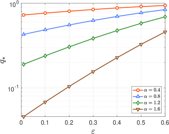
(44) 𝔼𝒙(m)<1+q(1p)2,subscript𝔼𝒙superscript𝑚1subscript𝑞superscript1subscript𝑝2\mathbb{E}_{\bm{x}}(m^{\ast})<1+\frac{q_{\ast}}{(1-p_{\ast})^{2}},

where the constants

p:=p(n,α,r,ε)=πn/2Γ(n/2)C~nα[B(α2,1α2)B(ε2r2;α2,1α2)],assignsubscript𝑝subscript𝑝𝑛𝛼𝑟𝜀superscript𝜋𝑛2Γ𝑛2subscriptsuperscript~𝐶𝛼𝑛delimited-[]𝐵𝛼21𝛼2𝐵superscript𝜀2superscript𝑟2𝛼21𝛼2\displaystyle p_{\ast}:=p_{\ast}(n,\alpha,r,\varepsilon)=\frac{\pi^{n/2}}{\Gamma(n/2)}\widetilde{C}^{\alpha}_{n}\Big{[}B\Big{(}\frac{\alpha}{2},1-\frac{\alpha}{2}\Big{)}-B\Big{(}\frac{\varepsilon^{2}}{r^{2}};\frac{\alpha}{2},1-\frac{\alpha}{2}\Big{)}\Big{]},
q:=q(n,α,r,ε)=1πn/2Γ(n/2)C~nα[B(α2,1α2)B((rε)2r2;α2,1α2)].assignsubscript𝑞subscript𝑞𝑛𝛼𝑟𝜀1superscript𝜋𝑛2Γ𝑛2subscriptsuperscript~𝐶𝛼𝑛delimited-[]𝐵𝛼21𝛼2𝐵superscript𝑟𝜀2superscript𝑟2𝛼21𝛼2\displaystyle q_{\ast}:=q_{\ast}(n,\alpha,r,\varepsilon)=1-\frac{\pi^{n/2}}{\Gamma(n/2)}\widetilde{C}^{\alpha}_{n}\Big{[}B\Big{(}\frac{\alpha}{2},1-\frac{\alpha}{2}\Big{)}-B\Big{(}\frac{(r-\varepsilon)^{2}}{r^{2}};\frac{\alpha}{2},1-\frac{\alpha}{2}\Big{)}\Big{]}.

with C~nαsubscriptsuperscript~𝐶𝛼𝑛\widetilde{C}^{\alpha}_{n} given in (11).

Proof 3.6.

Denote by 𝔹din,𝐱isuperscriptsubscript𝔹subscript𝑑𝑖𝑛subscript𝐱𝑖\mathbb{B}_{d_{i}}^{n,\bm{x}_{i}} the i𝑖i-th inside ball centered at 𝐱isubscript𝐱𝑖\bm{x}_{i} and tangent the domain ΓεsubscriptΓ𝜀\Gamma_{\varepsilon}, that is, the ball 𝔹din,𝐱isuperscriptsubscript𝔹subscript𝑑𝑖𝑛subscript𝐱𝑖\mathbb{B}_{d_{i}}^{n,\bm{x}_{i}} tangent the boundary 𝔹rεnsubscriptsuperscript𝔹𝑛𝑟𝜀\partial\mathbb{B}^{n}_{r-\varepsilon}. Then, it is easy to check that the radius of the i𝑖i-th ball is di=r|𝐱i|εsubscript𝑑𝑖𝑟subscript𝐱𝑖𝜀d_{i}=r-|\bm{x}_{i}|-\varepsilon. We set p(di,𝐱i,𝐲i)=Pr{𝐲i𝔹rεn𝔹din,𝐱i|𝐱i𝔹din,𝐱i}𝑝subscript𝑑𝑖subscript𝐱𝑖subscript𝐲𝑖Prconditional-setsubscript𝐲𝑖subscriptsuperscript𝔹𝑛𝑟𝜀superscriptsubscript𝔹subscript𝑑𝑖𝑛subscript𝐱𝑖subscript𝐱𝑖subscriptsuperscript𝔹𝑛subscript𝐱𝑖subscript𝑑𝑖p(d_{i},\bm{x}_{i},\bm{y}_{i})=\text{Pr}\{\bm{y}_{i}\in\mathbb{B}^{n}_{r-\varepsilon}\setminus\mathbb{B}_{d_{i}}^{n,\bm{x}_{i}}|\bm{x}_{i}\in\mathbb{B}^{n,\bm{x}_{i}}_{d_{i}}\}, which represents the probability that the (i+1)𝑖1(i+1)-th ball remains inside the region 𝔹rεnsubscriptsuperscript𝔹𝑛𝑟𝜀\mathbb{B}^{n}_{r-\varepsilon} under the condition that the i𝑖i-th ball is inside the region 𝔹rεnsubscriptsuperscript𝔹𝑛𝑟𝜀\mathbb{B}^{n}_{r-\varepsilon}. By (30), we have

p(di,𝒙i,𝒚i)=di<|𝒚i|<rεPdi(𝒙i,𝒚i)d𝒚i=πn/2Γ(n/2)C~nα[B(α2,1α2)B(di2(rε)2;α2,1α2)].𝑝subscript𝑑𝑖subscript𝒙𝑖subscript𝒚𝑖subscriptsubscript𝑑𝑖subscript𝒚𝑖𝑟𝜀subscript𝑃subscript𝑑𝑖subscript𝒙𝑖subscript𝒚𝑖differential-dsubscript𝒚𝑖superscript𝜋𝑛2Γ𝑛2subscriptsuperscript~𝐶𝛼𝑛delimited-[]𝐵𝛼21𝛼2𝐵superscriptsubscript𝑑𝑖2superscript𝑟𝜀2𝛼21𝛼2p(d_{i},\bm{x}_{i},\bm{y}_{i})=\int_{d_{i}<|\bm{y}_{i}|<r-\varepsilon}P_{d_{i}}(\bm{x}_{i},\bm{y}_{i})\,\mathrm{d}\bm{y}_{i}=\frac{\pi^{n/2}}{\Gamma(n/2)}\widetilde{C}^{\alpha}_{n}\Big{[}B\Big{(}\frac{\alpha}{2},1-\frac{\alpha}{2}\Big{)}-B\Big{(}\frac{d_{i}^{2}}{(r-\varepsilon)^{2}};\frac{\alpha}{2},1-\frac{\alpha}{2}\Big{)}\Big{]}.

To simplify the notations, we use pi=p(di,𝐱i,𝐲i)(0,1)subscript𝑝𝑖𝑝subscript𝑑𝑖subscript𝐱𝑖subscript𝐲𝑖01p_{i}=p(d_{i},\bm{x}_{i},\bm{y}_{i})\in(0,1), and qi=1pisubscript𝑞𝑖1subscript𝑝𝑖q_{i}=1-p_{i}, then

𝔼𝒙(m)=k=1Mk𝒙(m=k)=q1+2p1q2+3p1p2q3++Mp1p2pM1qM=k=1Mki=1k1piqk=k=1Mki=1k1πn/2Γ(n/2)C~nα[B(α2,1α2)B(di2(rε)2;α2,1α2)]{1πn/2Γ(n/2)C~nα[B(α2,1α2)B(dk2(rε)2;α2,1α2)]}.\begin{split}\mathbb{E}_{\bm{x}}(m^{\ast})&=\sum_{k=1}^{M}k\mathbb{P}_{\bm{x}}(m^{\ast}=k)=q_{1}+2p_{1}q_{2}+3p_{1}p_{2}q_{3}+\cdots+Mp_{1}p_{2}\cdots p_{M-1}q_{M}=\sum_{k=1}^{M}k\prod_{i=1}^{k-1}p_{i}q_{k}\\ &=\sum_{k=1}^{M}k\prod_{i=1}^{k-1}\frac{\pi^{n/2}}{\Gamma(n/2)}\widetilde{C}^{\alpha}_{n}\Big{[}B\Big{(}\frac{\alpha}{2},1-\frac{\alpha}{2}\Big{)}-B\Big{(}\frac{d_{i}^{2}}{(r-\varepsilon)^{2}};\frac{\alpha}{2},1-\frac{\alpha}{2}\Big{)}\Big{]}\\ &\,\,\,\,\,\,\,\,\,\cdot\Big{\{}1-\frac{\pi^{n/2}}{\Gamma(n/2)}\widetilde{C}^{\alpha}_{n}\Big{[}B\Big{(}\frac{\alpha}{2},1-\frac{\alpha}{2}\Big{)}-B\Big{(}\frac{d_{k}^{2}}{(r-\varepsilon)^{2}};\frac{\alpha}{2},1-\frac{\alpha}{2}\Big{)}\Big{]}\Big{\}}.\end{split}

Let p=maxi{pi}subscript𝑝subscript𝑖subscript𝑝𝑖p_{\ast}=\displaystyle\max_{i}\{p_{i}\} and q=maxi{qj}subscript𝑞subscript𝑖subscript𝑞𝑗q_{\ast}=\displaystyle\max_{i}\{q_{j}\}, it is easy to verify that

𝔼x(m)subscript𝔼𝑥superscript𝑚\displaystyle\mathbb{E}_{x}(m^{\ast}) <q1+2p1q+3p1pq+4p1p2q++Mp1pM1qabsentsubscript𝑞12subscript𝑝1subscript𝑞3subscript𝑝1subscript𝑝subscript𝑞4subscript𝑝1superscriptsubscript𝑝2subscript𝑞𝑀subscript𝑝1superscriptsubscript𝑝𝑀1subscript𝑞\displaystyle<q_{1}+2p_{1}q_{\ast}+3p_{1}p_{\ast}q_{\ast}+4p_{1}p_{\ast}^{2}q_{\ast}+\cdots+Mp_{1}p_{\ast}^{M-1}q_{\ast}
=12p1+p1(1+2q+3pq+4p2q++MpM1q)absent12subscript𝑝1subscript𝑝112subscript𝑞3subscript𝑝subscript𝑞4superscriptsubscript𝑝2subscript𝑞𝑀superscriptsubscript𝑝𝑀1subscript𝑞\displaystyle=1-2p_{1}+p_{1}\big{(}1+2q_{\ast}+3p_{\ast}q_{\ast}+4p_{\ast}^{2}q_{\ast}+\cdots+Mp_{\ast}^{M-1}q_{\ast}\big{)}
=12p1+p1(1+qp(1+2p+3p2+4p3++MpM1)qp)absent12subscript𝑝1subscript𝑝11subscript𝑞subscript𝑝12subscript𝑝3superscriptsubscript𝑝24superscriptsubscript𝑝3𝑀superscriptsubscript𝑝𝑀1subscript𝑞subscript𝑝\displaystyle=1-2p_{1}+p_{1}\Big{(}1+\frac{q_{\ast}}{p_{\ast}}\big{(}1+2p_{\ast}+3p_{\ast}^{2}+4p_{\ast}^{3}+\cdots+Mp_{\ast}^{M-1}\big{)}-\frac{q_{\ast}}{p_{\ast}}\Big{)}
=12p1+p1(1+qpp(p+p2+p3+p4++pM)qp)absent12subscript𝑝1subscript𝑝11subscript𝑞subscript𝑝subscriptsubscript𝑝subscript𝑝superscriptsubscript𝑝2superscriptsubscript𝑝3superscriptsubscript𝑝4superscriptsubscript𝑝𝑀subscript𝑞subscript𝑝\displaystyle=1-2p_{1}+p_{1}\Big{(}1+\frac{q_{\ast}}{p_{\ast}}\,\partial_{p_{\ast}}\!\big{(}p_{\ast}+p_{\ast}^{2}+p_{\ast}^{3}+p_{\ast}^{4}+\cdots+p_{\ast}^{M}\big{)}-\frac{q_{\ast}}{p_{\ast}}\Big{)}
=12p1+p1(1+qpp(p(1pM)1p)qp).absent12subscript𝑝1subscript𝑝11subscript𝑞subscript𝑝subscriptsubscript𝑝subscript𝑝1superscriptsubscript𝑝𝑀1subscript𝑝subscript𝑞subscript𝑝\displaystyle=1-2p_{1}+p_{1}\Big{(}1+\frac{q_{\ast}}{p_{\ast}}\,\partial_{p_{\ast}}\!\Big{(}\frac{p_{\ast}(1-p_{\ast}^{M})}{1-p_{\ast}}\Big{)}-\frac{q_{\ast}}{p_{\ast}}\Big{)}.

As 0<p,q<1formulae-sequence0subscript𝑝subscript𝑞10<p_{\ast},q_{\ast}<1, it is evident that pM0superscriptsubscript𝑝𝑀0p_{\ast}^{M}\to 0 for M𝑀M\to\infty, which implies p(1pM)1pp1psubscript𝑝1superscriptsubscript𝑝𝑀1subscript𝑝subscript𝑝1subscript𝑝\frac{p_{\ast}(1-p_{\ast}^{M})}{1-p_{\ast}}\to\frac{p_{\ast}}{1-p_{\ast}}. A direct computation gives p(p1p)=1(1p)2subscriptsubscript𝑝subscript𝑝1subscript𝑝1superscript1subscript𝑝2\partial_{p_{\ast}}(\frac{p_{\ast}}{1-p_{\ast}})=\frac{1}{(1-p_{\ast})^{2}}, then we find from (3.6) that

𝔼𝒙(m)<1p1+p1qp(1p)2<1+p1qp(1p)2<1+q(1p)2,subscript𝔼𝒙superscript𝑚1subscript𝑝1subscript𝑝1subscript𝑞subscript𝑝superscript1subscript𝑝21subscript𝑝1subscript𝑞subscript𝑝superscript1subscript𝑝21subscript𝑞superscript1subscript𝑝2\mathbb{E}_{\bm{x}}(m^{\ast})<1-p_{1}+\frac{p_{1}\,q_{\ast}}{p_{\ast}(1-p_{\ast})^{2}}<1+\frac{p_{1}\,q_{\ast}}{p_{\ast}(1-p_{\ast})^{2}}<1+\frac{q_{\ast}}{(1-p_{\ast})^{2}},

where we used the fact that p1<psubscript𝑝1subscript𝑝p_{1}<p_{*} in the last inequality. This ends the proof.
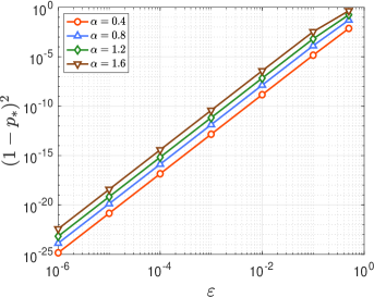
Refer to caption
Refer to caption
Figure 4: Left: the value 1p21subscriptsuperscript𝑝21-p^{2}_{\ast} versus ε𝜀\varepsilon; Right: the value qsubscript𝑞q_{\ast} versus ε𝜀\varepsilon.

In Fig. 4, we plot the magnitude of (1p)2superscript1subscript𝑝2(1-p_{\ast})^{2} and qsubscript𝑞q_{\ast} against various ε𝜀\varepsilon in the log-log and semi-log scale, respectively. We observe that the values of (1p)2superscript1subscript𝑝2(1-p_{\ast})^{2} and qsubscript𝑞q_{\ast} increase as ε𝜀\varepsilon increase. They indicate that the greater the width ε𝜀\varepsilon, the lower the probability that the ball in the domain ΩΩ\Omega will remain in the next step. On the contrary, the thicker the width ε𝜀\varepsilon, the higher probability the small ball will leave the domain ΩΩ\Omega in the next step. We observe that they are consistent with the theoretical result.

4 Numerical Results

We present ample numerical results to illustrate our numerical methods, in particular, the Algorithm 1 for computing solutions of fractional Poisson equation (3). These examples include smooth functions and functions with low regularities at the boundary, and we also checked the efficiency of the proposed method in two dimensions and even in 101010-dimensions. Note that all computations below were performed in MATLAB R2018a on a 64-bit Macbook Pro laptop with a quad-core Intel Core i5 processor at 2.3 GHz and 8GB of RAM. For the sake of simplicity, we work on the problem with exact solutions. In what follows, all the numerical results are obtained by Algorithm 1, and all the numerical errors are computed via randomly selected points {𝒙i}i=1Nsuperscriptsubscriptsubscript𝒙𝑖𝑖1𝑁\{\bm{x}_{i}\}_{i=1}^{N} with N=10000𝑁10000N=10000 as below

Error=1N(i=1N(u(𝒙i)u(𝒙i))2)12,Error1𝑁superscriptsuperscriptsubscript𝑖1𝑁superscript𝑢subscript𝒙𝑖subscript𝑢subscript𝒙𝑖212\text{Error}=\frac{1}{N}\Big{(}\sum_{i=1}^{N}(u(\bm{x}_{i})-u_{\ast}(\bm{x}_{i}))^{2}\Big{)}^{\frac{1}{2}},

where u(𝒙)subscript𝑢𝒙u_{\ast}(\bm{x}) denote the numerical solution. The other parameter are set to be ε=106𝜀superscript106\varepsilon=10^{-6}.

Example 1.

(Exact solution in 2D with homogeneous BCs) We first consider (3) on a unit disk Ω=𝔹12Ωsubscriptsuperscript𝔹21\Omega=\mathbb{B}^{2}_{1} with the following exact solutions:

(46) u(𝒙)=(1|𝒙|2)+α2,𝑢𝒙subscriptsuperscript1superscript𝒙2𝛼2u(\bm{x})=(1-|\bm{x}|^{2})^{\frac{\alpha}{2}}_{+},\;\;\;

where a+=max{a,0}subscript𝑎𝑎0a_{+}=\max\{a,0\}. According to [16], the source term reduce to a constant, i.e., f=2αΓ2(α2+1).𝑓superscript2𝛼superscriptΓ2𝛼21f=2^{\alpha}\Gamma^{2}(\frac{\alpha}{2}+1). In this case, the nonlocal boundary condition becomes homogeneous, that is, g(𝐱)=0𝑔𝐱0g(\bm{x})=0 in ΩcsuperscriptΩ𝑐\Omega^{c}.

Refer to caption
(a) α=0.4𝛼0.4\alpha=0.4
Refer to caption
(b) α=0.8𝛼0.8\alpha=0.8
Refer to caption
(c) α=1.2𝛼1.2\alpha=1.2
Refer to caption
(d) α=1.6𝛼1.6\alpha=1.6
Figure 5: Profiles of the numerical solutions with various α𝛼\alpha.

In order to demonstrate the efficiency of the proposed algorithm, we plot in Fig. 5 the profiles of numerical solutions with α=0.4, 0.8, 1.2, 1.6𝛼0.40.81.21.6\alpha=0.4,\,0.8,\,1.2,\,1.6, in which we compute the approximate result at each given point 𝒙=(x1,x2)𝒙subscript𝑥1subscript𝑥2\bm{x}=(x_{1},x_{2}) by employing 5000 paths. The exact solution has singularity near the boundary and behaves like dist(𝒙,Ω)α2distsuperscript𝒙Ω𝛼2{\rm dist}(\bm{x},\partial\Omega)^{\frac{\alpha}{2}}, where dist(𝒙,Ω)dist𝒙Ω{\rm dist}(\bm{x},\partial\Omega) denotes the distance function from 𝒙𝒙\bm{x} to the boundary ΩΩ\partial\Omega. It can be seen from Fig. 5, with the decrease of the index α𝛼\alpha, the singular layers near the boundary are thinner and sharper as expected. We note that the computational complexity of the algorithm is 𝒪(N)𝒪𝑁\mathcal{O}(N), where N𝑁N represents the number of paths we set.
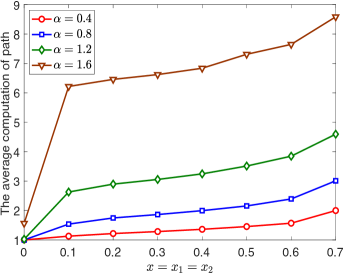
Refer to caption
Refer to caption
Figure 6: Simulation for two-dimension. Left: the average number of steps for fixed point with various α𝛼\alpha; Right: numerical errors against ε𝜀\varepsilon.

In Fig. 6 (left), we shows the average number of iterations required for each path when calculating u(𝒙)𝑢𝒙u(\bm{x}) with different α𝛼\alpha, that is, the average of steps required for point 𝒙𝒙\bm{x} to escape from domain 𝔹12superscriptsubscript𝔹12\mathbb{B}_{1}^{2}. We observe that when the starting point is farther away from the center, it will need more iterations, as the corresponding circle is smaller for the point near the boundary. In other words, the larger the area of 𝔹12𝔹r12subscriptsuperscript𝔹21subscriptsuperscript𝔹2subscript𝑟1\mathbb{B}^{2}_{1}\setminus\mathbb{B}^{2}_{r_{1}} will be, and the more likely the next point will fall in this area. In addition, when all conditions are set to be the same, as expected, the number of iterations increases as α𝛼\alpha increases. As α𝛼\alpha tends to 222, the distance from a fixed point 𝒙𝒙\bm{x} to the next point will be smaller, which leads to an increase in the number of iterations escaping from region 𝔹12subscriptsuperscript𝔹21\mathbb{B}^{2}_{1}. In Fig. 6 (right), we plot the numerical errors, in log-log scale, against the number of paths with different fractional order α𝛼\alpha.

Example 2.

(Source problem in 2D with non-homogeneous BCs) We next consider (3) with the following source functions:

(47) f(𝒙)=Γ(2+α)2F1(2+α2,3+α2;1;|𝒙|2),onΩ=𝔹12.formulae-sequence𝑓𝒙Γsubscript2𝛼2subscript𝐹12𝛼23𝛼21superscript𝒙2onΩsubscriptsuperscript𝔹21f(\bm{x})=\Gamma(2+\alpha)_{2}F_{1}\Big{(}\frac{2+\alpha}{2},\frac{3+\alpha}{2};1;-|\bm{x}|^{2}\Big{)},\;\;{\rm on}\;\Omega=\mathbb{B}^{2}_{1}.

Fortunately, we have the explicit expression of exact solution u(𝐱)=(1+|𝐱|2)32𝑢𝐱superscript1superscript𝐱232u(\bm{x})=(1+|\bm{x}|^{2})^{-\frac{3}{2}} on 2,superscript2\mathbb{R}^{2}, which implies the nonhomegeneous boundary condition g(𝐱)=u(𝐱)𝑔𝐱𝑢𝐱g(\bm{x})=u(\bm{x}) on ΩcsuperscriptΩ𝑐\Omega^{c}.

Refer to caption
Refer to caption
Figure 7: Simulation for two-dimension. Left: the average number of steps for fixed point with various α𝛼\alpha; Right: numerical errors against the number of path with various α𝛼\alpha.

We use the Monte Carlo method suggested in Algorithm 1 to resolve this problem. In Fig. 7 (left), we plot the average number of iterations required for each path to simulate u(𝒙)𝑢𝒙u(\bm{x}) with various fractional order α𝛼\alpha. The errors of numerical solution against the number of path with various α𝛼\alpha in log-log scale are shown in Fig. 7 (right). We observe that the numerical errors decay as the number of path increases. They indicate that our algorithm is very effective for IFL with nonhomogeneous BCs.
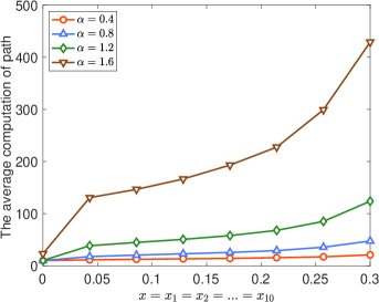
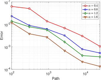
Refer to caption
Refer to caption
Figure 8: Simulation for 101010-dimension. Left: the average number of steps for fixed point with various α𝛼\alpha; Right: numerical errors against the number of path with various α𝛼\alpha.
Example 3.

(Exact solution in 10D with homogeneous BCs) Again, we consider (3) in high dimensions with the following exact solutions (cf. [16]):

(48) u(𝒙)=(1|𝒙|)+α2,𝒙Ω=𝔹110,formulae-sequence𝑢𝒙subscriptsuperscript1𝒙𝛼2𝒙Ωsubscriptsuperscript𝔹101u(\bm{x})=(1-|\bm{x}|)^{\frac{\alpha}{2}}_{+},\;\;\bm{x}\in\Omega=\mathbb{B}^{10}_{1},

then the source term reduce to a constant, i.e., f(𝐱)=2αΓ(1+α2)Γ(n+α2)/Γ(n2).𝑓𝐱superscript2𝛼Γ1𝛼2Γ𝑛𝛼2Γ𝑛2f(\bm{x})=2^{\alpha}\Gamma(1+\frac{\alpha}{2})\Gamma(\frac{n+\alpha}{2})/\Gamma(\frac{n}{2}). In this case, the nonlocal boundary condition is homogeneous, that is, g(𝐱)=0𝑔𝐱0g(\bm{x})=0 in ΩcsuperscriptΩ𝑐\Omega^{c}.

In Fig. 8 (left), we plot the average number of iterations required for each path when calculating u(𝒙)𝑢𝒙u(\bm{x}) for different α𝛼\alpha. The numerical errors of numerical solution against the number of path with various α𝛼\alpha in log-log scale are plotted in Fig. 8 (right). As with the results in 2D, Fig. 8 demonstrate that the average number of iterations required to compute u(𝒙)𝑢𝒙u(\bm{x}) for the same α𝛼\alpha increases as |𝒙|𝒙|\bm{x}| increases for 10-dimensional problems. For a given point 𝒙Ω𝒙Ω\bm{x}\in\Omega, the average number of iterations required increases in proportion to the value of fractional order α𝛼\alpha. Moreover, the relationship between the number of paths and numerical error is consistent with the two-dimensional problem. In particular, they indicate that our algorithm is very effective and stable for high dimensional problems. Indeed, this is one of the main advantages of the proposed method, which distinguish our approach from other existing methods for fractional PDEs.

Example 4.

(IFL on irregular domains) In this example, we shall present the numerical results of our algorithm for IFL on irregular domains. To check the accuracy, we consider (3) with the following source function and boundary condition:

(49) f(𝒙)=2αΓ(1+α/2)1F1(2+α2;1;|𝒙|2),𝒙Ω;g(𝒙)=e|𝒙|2,𝒙Ωc.formulae-sequence𝑓𝒙superscript2𝛼Γsubscript1𝛼21subscript𝐹12𝛼21superscript𝒙2formulae-sequence𝒙Ωformulae-sequence𝑔𝒙superscript𝑒superscript𝒙2𝒙superscriptΩ𝑐f(\bm{x})=2^{\alpha}\Gamma(1+\alpha/2)_{1}F_{1}\Big{(}\frac{2+\alpha}{2};1;-|\bm{x}|^{2}\Big{)},\;\;\bm{x}\in\Omega;\;\;\;g(\bm{x})=e^{-|\bm{x}|^{2}},\;\;\bm{x}\in\Omega^{c}.

In this case, we take Ω=[1,1]2(0,1]2Ωsuperscript112superscript012\Omega=[-1,1]^{2}\setminus(0,1]^{2}, which represents an L-shaped domain. According to [34], we have the explicit expression of exact solution u(𝐱)=e|𝐱|2𝑢𝐱superscript𝑒superscript𝐱2u(\bm{x})=e^{-|\bm{x}|^{2}} on Ω.Ω\Omega.

Refer to caption
Refer to caption
Figure 9: Simulation for two-dimension on complex domains. Left: the average number of steps for fixed point with various α𝛼\alpha; Right: numerical errors against the number of path with various α𝛼\alpha.

In Fig. 9 (left), we show the average number of iterations required for each path when calculating u(𝒙)𝑢𝒙u(\bm{x}) for different fractional power α𝛼\alpha. We observe from Fig. 9 (left) that the average number of iterations for each path does not increase when |𝒙|>0.1𝒙0.1|\bm{x}|>0.1. For the L𝐿L-shaped domain, with the increase of the coordinates of point 𝒙𝒙\bm{x} along with the (1,1)11(1,-1)-direction, the distance between the point and boundary first increases and then gradually decreases. Thus, the average number of iterations required for each path first increases and then gradually decreases. The numerical errors against the path number is listed in Fig. 9 (right). As excepted, the numerical errors decay algebraically as the increase of the total path. These are consistent with our previous theoretical analysis results.

To show the efficiency of our method on the complex domains, we further consider the following three cases:

(i).For the stripe domain, we take

(50) f(𝒙)=2αΓ(1+α2)(cosα3(c2𝒙)+sinα2(c1𝒙))cos(|𝒙|2)onΩ,𝑓𝒙superscript2𝛼Γ1𝛼2superscript𝛼3subscript𝑐2𝒙superscript𝛼2subscript𝑐1𝒙superscript𝒙2onΩf(\bm{x})=2^{\alpha}\Gamma(1+\frac{\alpha}{2})(\cos^{\frac{\alpha}{3}}(c_{2}\bm{x})+\sin^{\frac{\alpha}{2}}(c_{1}\bm{x}))\cos(-|\bm{x}|^{2})\;\;{\rm on}\;\Omega,

where c1=(π3,π4)subscript𝑐1𝜋3𝜋4c_{1}=(\frac{\pi}{3},-\frac{\pi}{4}), c2=(π2,2π3)subscript𝑐2𝜋22𝜋3c_{2}=(-\frac{\pi}{2},\frac{2\pi}{3}), 𝒙=(x1,x2)T𝒙superscriptsubscript𝑥1subscript𝑥2𝑇\bm{x}=(x_{1},x_{2})^{T}, and ΩΩ\Omega is the stripe domain on [5,5]×[0.5,0.5]550.50.5[-5,5]\times[-0.5,0.5], the boundary condition can be set as g(𝒙)=0𝑔𝒙0g(\bm{x})=0 over ΩcsuperscriptΩ𝑐\Omega^{c}.

(ii).For regular hexagon domain, we take

(51) f(𝒙)=sin2(c1𝒙)+cos2(c2𝒙)(αx1x2)3,onΩ,𝑓𝒙superscript2subscript𝑐1𝒙superscript2subscript𝑐2𝒙superscript𝛼subscript𝑥1subscript𝑥23onΩf(\bm{x})=\sin^{2}(c_{1}\bm{x})+\cos^{2}(c_{2}\bm{x})-(\alpha x_{1}x_{2})^{3},\;\;{\rm on}\;\Omega,

where ΩΩ\Omega is the regular hexagon domain on [1,1]2superscript112[-1,1]^{2}, the boundary condition can be set as g(𝒙)=0𝑔𝒙0g(\bm{x})=0 over ΩcsuperscriptΩ𝑐\Omega^{c}.

(iii).For the annulus domain, we take

(52) f(𝒙)=cos(x222x1x2)sin(x12+2x1x2),onΩ,𝑓𝒙superscriptsubscript𝑥222subscript𝑥1subscript𝑥2superscriptsubscript𝑥122subscript𝑥1subscript𝑥2onΩf(\bm{x})=\cos(x_{2}^{2}-2x_{1}x_{2})-\sin(x_{1}^{2}+2x_{1}x_{2}),\;\;{\rm on}\;\Omega,

where Ω={𝒙2:0.3<|𝒙|2<1}Ωconditional-set𝒙superscript20.3superscript𝒙21\Omega=\{\bm{x}\in\mathbb{R}^{2}:0.3<|\bm{x}|^{2}<1\} is the annulus domain, the boundary condition can be set as g(𝒙)=0𝑔𝒙0g(\bm{x})=0 over ΩcsuperscriptΩ𝑐\Omega^{c}.

Refer to caption
Refer to caption
Refer to caption
Refer to caption
Figure 10: Profiles of the numerical solutions zoomed in the stripe domain [5,5]×[0.5,0.5]550.50.5[-5,5]\times[-0.5,0.5] with α=0.4,0.8,1.2,1.6𝛼0.40.81.21.6\alpha=0.4,0.8,1.2,1.6 (from top to bottom).
Refer to caption
(a) α=0.4𝛼0.4\alpha=0.4
Refer to caption
(b) α=0.8𝛼0.8\alpha=0.8
Refer to caption
(c) α=1.2𝛼1.2\alpha=1.2
Refer to caption
(d) α=1.6𝛼1.6\alpha=1.6
Refer to caption
(e) α=0.4𝛼0.4\alpha=0.4
Refer to caption
(f) α=0.8𝛼0.8\alpha=0.8
Refer to caption
(g) α=1.2𝛼1.2\alpha=1.2
Refer to caption
(h) α=1.6𝛼1.6\alpha=1.6
Figure 11: Profiles of the numerical solutions with various α𝛼\alpha. Top: zoomed in the hexagon domain; Botton: zoomed in the annulus domain.

We use the proposed Monte Carlo method to calculate numerical solutions on three different shaped domains, and plot the corresponding profiles with varous fractional order α𝛼\alpha in Fig. 10 and 11. We observe similar behaviors as in the circular domain case, and the singularity layer near the boundary becomes thinner as expected as the fractional power α𝛼\alpha decreases.

5 Conclusion

This paper proposes an efficient Monte Carlo method for solving fractional PDEs on bounded domains in arbitrary dimensions. The key to the efficiency of the Monte Carlo algorithm is to construct a new Feynman-Kac representation in expectation form based on the explicit expressions of the Green functions. Then, we can avoid calculating the complex integrals associated with α𝛼\alpha-stable process function. The representation (18) allows us only to calculate the expectation of a random variable with known density functions, which enjoys the explicit expression of the Green functions. Each jump in the angular direction is distributed uniformly with the aid of the spherical coordinates, so we only need to appropriately add sample nodes in the angular direction with the increased dimensions. Consequently, the computation time will increase at a moderate pace with the increase of dimensions. Thus, this new process possesses fascinating merits for solving high-dimensional problems. More importantly, we prove the efficiency of our algorithm and establish the error analysis of the proposed method for the fractional Poisson equation. Our numerical experiments demonstrate that our algorithms are efficient and accurate. In addition, the Monte Carlo method allows us to use parallel computing to improve the calculation efficiency and significantly reduce the computation time.

The idea of the proposed Monte Carlo method can be extended to the time-dependent problems with Feynman-Kac representation in a similar setting. In the future, we can combine the proposed method with the deep neural network for solving the nonlocal models driven by a stochastic process.

Acknowledgments

C. Sheng would like to thank Professor Jie Shen at Purdue University for many valuable suggestions and enlightening discussions.

References

  • [1] G. Acosta and J. P. Borthagaray, A fractional Laplace equation: regularity of solutions and finite element approximations, SIAM J. Numer. Anal., 55 (2017), pp. 472–495.
  • [2] M. Ainsworth and C. Glusa, Aspects of an adaptive finite element method for the fractional Laplacian: a priori and a posteriori error estimates, efficient implementation and multigrid solver, Comput. Methods Appl. Mech. Engrg., 327 (2017), pp. 4–35.
  • [3] Janicki Aleksander and Weron Aleksander, Can one see α𝛼\alpha-stable variables and processes?, Statist. Sci., 9 (1994), pp. 109–126.
  • [4] A. Bonito, W. Lei, and J. E. Pasciak, Numerical approximation of the integral fractional Laplacian, Numer. Math., 142 (2019), pp. 235–278.
  • [5] J. P. Borthagaray, L. M. Del Pezzo, and S. Martinez, Finite element approximation for the fractional eigenvalue problem, J. Sci. Comput., 77 (2018), pp. 308–329.
  • [6] J. P. Borthagaray, D. Leykekhman, and R. H. Nochetto, Local energy estimates for the fractional Laplacian, SIAM J. Numer. Anal., 59 (2021), pp. 1918–1947.
  • [7] D. Brockmann, L. Hufnagel, and T. Geisel, The scaling laws of human travel, Nature, 439 (2006), p. 462.
  • [8] C. Bucur, Some observations on the Green function for the ball in the fractional Laplace framework, Commun. Pure Appl. Anal., 15 (2016), pp. 657–699.
  • [9] H. Chen, Y. Yu, J. Jaworski, N. Trask, and M. D’Elia, Data-driven learning of reynolds stress tensor using nonlocal models, Bulletin of the American Physical Society, 66 (2021).
  • [10] L. Chen, Z. Mao, and H. Li, Jacobi-Galerkin spectral method for eigenvalue problems of Riesz fractional differential equations, arXiv preprint arXiv:1803.03556, (2018).
  • [11] K. L. Chung and Z. X. Zhao, From Brownian motion to Schrödinger’s equation, vol. 312 of Grundlehren der mathematischen Wissenschaften [Fundamental Principles of Mathematical Sciences], Springer-Verlag, Berlin, 1995.
  • [12] M. Day, Book Review: Functional integration and partial differential equations, Bull. Amer. Math. Soc. (N.S.), 17 (1987), pp. 346–351.
  • [13] J. M. DeLaurentis and L. A. Romero, A Monte Carlo method for Poisson’s equation, J. Comput. Phys., 90 (1990), pp. 123–140.
  • [14] S. Duo and Y. Zhang, Computing the ground and first excited states of the fractional Schrödinger equation in an infinite potential well, Commun. Comput. Phys., 18 (2015), pp. 321–350.
  • [15]  , Accurate numerical methods for two and three dimensional integral fractional Laplacian with applications. Comput. Methods Appl. Mech. Engrg., 355 (2019), pp. 639-662.
  • [16] B. O. Dyda, A. Kuznetsov, and M. Kwaśnicki, Fractional Laplace operator and Meijer G-function, Constr. Approx., 45 (2017), pp. 427–448.
  • [17] M. Faustmann, M. Karkulik, and J. M. Melenk, Local convergence of the FEM for the integral fractional Laplacian, arXiv preprint arXiv:2005.14109, (2020).
  • [18] A. Friedman, Stochastic differential equations and applications. Vol. 2, Probability and Mathematical Statistics, Vol. 28, Academic Press [Harcourt Brace Jovanovich, Publishers], New York-London, 1976.
  • [19] M. Gulian, M. Raissi, P. Perdikaris, and G. Karniadakis, Machine learning of space-fractional differential equations, SIAM Journal on Scientific Computing, 41 (2019), pp. A2485–A2509.
  • [20] L. Guo, H. Wu, X. Yu, and T. Zhou, Monte Carlo PINNs: deep learning approach for forward and inverse problems involving high dimensional fractional partial differential equations, arXiv preprint arXiv:2203.08501, (2022).
  • [21] Z. Hao, H. Li, Z. Zhang, and Z. Zhang, Sharp error estimates of a spectral Galerkin method for a diffusion-reaction equation with integral fractional Laplacian on a disk, Math. Comp., 90 (2021), pp. 2107–2135.
  • [22] Z. Hao and Z. Zhang, Optimal regularity and error estimates of a spectral Galerkin method for fractional advection-diffusion-reaction equations, SIAM J. Numer. Anal., 58 (2020), pp. 211–233.
  • [23] Z. Hao, Z. Zhang, and R. Du, Fractional centered difference scheme for high-dimensional integral fractional Laplacian, J. Comput. Phys., 424 (2021), p. 109851.
  • [24] A. E. Kyprianou, A. Osojnik, and T. Shardlow, Unbiased ‘walk-on-spheres’ Monte Carlo methods for the fractional Laplacian, IMA J. Numer. Anal., 38 (2018), pp. 1550–1578.
  • [25] Z. Mao, Z. Li, and G. E. Karniadakis, Nonlocal flocking dynamics: Learning the fractional order of PDEs from particle simulations, Commun. Appl. Math. Comput., 1 (2019), pp. 579–619.
  • [26] Z. Mao and J. Shen, Hermite spectral methods for fractional PDEs in unbounded domains, SIAM J. Sci. Comput., 39 (2017), pp. A1928–A1950.
  • [27] R. Metzler and J. Klafter, The random walk’s guide to anomalous diffusion: a fractional dynamics approach, Phys. Rep., 339 (2000), pp. 1–77.
  • [28] R. Metzler and J. Klafter, Joseph, The restaurant at the end of the random walk: recent developments in the description of anomalous transport by fractional dynamics, J. Phys. A, 37 (2004), p. R161.
  • [29] V. Minden and L. Ying, A simple solver for the fractional Laplacian in multiple dimensions, SIAM J. Sci. Comput., 42 (2020), pp. A878–A900.
  • [30] E. D. Nezza, G. Palatucci, and E. Valdinoci, Hitchhiker’s guide to the fractional Sobolev spaces, Bull. Sci. Math., 136 (2012), pp. 521–573.
  • [31] G. Pang, L. Lu, and G. E. Karniadakis, fpinns: Fractional physics-informed neural networks, SIAM Journal on Scientific Computing, 41 (2019), pp. A2603–A2626.
  • [32] G. Pang, M. D’Elia, M. Parks, and G. Karniadakis, npinns: Nonlocal physics-informed neural networks for a parametrized nonlocal universal laplacian operator. algorithms and applications, Journal of Computational Physics, 422 (2020), p. 109760.
  • [33] T. Shardlow, A walk outside spheres for the fractional Laplacian: fields and first eigenvalue, Math. Comp., 88 (2019), pp. 2767–2792.
  • [34] C. Sheng, J. Shen, T. Tang, L.-L. Wang, and H. Yuan, Fast Fourier-like mapped Chebyshev spectral-Galerkin methods for PDEs with integral fractional Laplacian in unbounded domains, SIAM J. Numer. Anal., 58 (2020), pp. 2435–2464.
  • [35] M. Shlesinger, B. West, and J. Klafter, Lévy dynamics of enhanced diffusion: Application to turbulence, Phys. Rev. Lett., 58 (1987), p. 1100.
  • [36] T. Tang, H. Yuan, and T. Zhou, Hermite spectral collocation methods for fractional PDEs in unbounded domains, Commun. Comput. Phys., 24 (2018), pp. 1143–1168.
  • [37] H. You, Y. Yu, M. D’Elia, T. Gao, and S. Silling, Nonlocal kernel network (NKN): a stable and resolution-independent deep neural network, arXiv preprint arXiv:2201.02217, (2022).
  • [38] E. C. Zachmanoglou and D. W. Thoe, Introduction to partial differential equations with applications, Dover Publications, Inc., New York, second ed., 1986.