Coulomb-Nuclear Interference: Theory and Practice for $pp$-Scattering at 13 TeV.

Abstract

We provide a detailed reconsideration of the theoretical basis for the treatment of Coulomb-nuclear interference (CNI) and a corresponding thorough analysis of the procedure of extraction of the basic parameters $\rho^{\leavevmode\nobreak\ pp},\sigma_{tot}^{\leavevmode\nobreak\ pp}$ and $B^{\leavevmode\nobreak\ pp}$ from the TOTEM data at $\sqrt{s}=13$ TeV. A more substantiated account of CNI, as well as an in-depth statistical analysis of the TOTEM data at low transferred momenta, give results that differ from those published by the TOTEM collaboration.

Introduction

Measurements by the LHC TOTEM Collaboration at 13 TeV [1] caused a number of papers with vivid discussions, often with opposite conclusions. The TOTEM Collaboration gives two values of the parameter

$$\rho=\frac{\mbox{Re}T_{N}(s,0)}{\mbox{Im}T_{N}(s,0)}=0.09\div 0.10$$

with a strikingly small error, less than $10\%$, although the very data show large systematic errors. An unexpectedly low value of $\rho$ given by the TOTEM prompted some authors to consider these results as a proof of the existence of the so-called ”Maximal Odderon” (in particular those of Ref.[2], in which $\rho$ was estimated as very close to $0.1$). Such an interpretation was adopted in [1] (with some reservation, though) as a first experimental observation of a ”3-gluon compound state”.

It was also claimed in [1] that such a low value of $\rho$ along with the mentioned narrow error corridor supposedly ”has implied the exclusion of all the models classified and published by”the COMPETE Group [3].

Concerning the credibility of the statement about the Odderon observation we refer the reader to Refs. [4] and [5]where a detailed discussion of this problem is given.

In the present work we concentrate on two important issues of the parameter retrieval from the data.

• First of all, this is a way of taking into account CNI effects in the full scattering amplitude. Beyond a simplistic adding the Coulomb 1-photon exchange to the nuclear amplitude (which is obviously theoretically untenable) we find in the literature two ways of accounting for CNI.

  The first one goes back to the pioneering work of H.Bethe and was significantly improved by D.R. Yennie and G.B. West [6]. The idea is that the inclusion of Coulomb exchanges leads to the appearance of an additional phase in the strong interaction scattering amplitude. Within a couple of decades this method served a convenient phenomenological tool for the description of the differential cross-section with account for CNI and extracting the parameters mentioned above (see e.g.[8]).

  Nonetheless, afterwards it was criticized by R.Cahn (and a dozen years later in a more detailed way by V. Kundrát and M. Lokajíček) [9]. It was noted that the Bethe-Yennie-West method requires the phase of the nuclear scattering amplitude $T_{N}$ to be independent of the momentum transferred which is a rather restrictive condition. Moreover, as was proved recently [10] , such an independence, even in an arbitrary narrow interval, leads to identical vanishing of this amplitude.In addition, it is noted in [11] that the form of the Coulomb phase proposed by Yennie and West contradicts the general properties of analyticity in the t-channel.

  As a replacement for the Bethe-Yennie-West method, a different method was proposed in [9] for taking into account the CNI effects, which does not impose unnecessary restrictions on the phase of the nuclear scattering amplitude. Exactly this method was adopted in [1] for retrieving the $\rho$-parameter etc which attracted a close attention.

  However, this last method, which we will call CKL (for Cahn-Kundrát-Lokajíček), although it has been qualified in [1] as ” the most general interference formula”, also turned out to be flawed. The problem was, in particular, in an oversimplified way of the form factor account.

  A formula devoid of this shortcoming was derived in Refs. [12], [13].

  In what follows we use an expression based on these latter papers for a correct account for CNI effects. We believe it is suitable for general use.

• The aforementioned low value of $\rho$ was obtained in [1] on the basis of an analysis of the differential cross-section at low values of the transferred momenta. To this end two arrays of the data were chosen. Specifically, the sets with $|t|\leq 0.15\leavevmode\nobreak\ \mbox{GeV}^{2}$ and with $|t|\leq 0.07\leavevmode\nobreak\ \mbox{GeV}^{2}$, though no reason why namely these values of cut-off were taken was given.

  Following the method of Ref.[1], we also use, when processing the data, a cut-off in $|t|$ but find that together with an upper cut-off one has to impose a lower cut-off as well, and in Section 3 we motivate our choice for both. The values of parameters ($\rho$, total cross-section $\sigma_{\mbox{tot}}$ and the forward slope $B$ of $d\sigma/dt$), retrieved with help of such a procedure, turn out to be different from those announced in [1].As regards the $\rho$ parameter, we find that the statistically justified retrieval leads inevitably to a significant widening of the error corridor what is of fundamental importance.

• The last item we would like to draw the attention to is the question: to which extent the smearing of the proton electric charge over its volume (embodied by the form factor $\mathcal{F}$) makes the parameters $\rho$ etc different from the idealized case of the point-like charge ($\mathcal{F}=1$)? The answer turned out to be quite surprising and quite helpful for estimate of accuracy of the cross-section description in the realistic case.

1 Exact formula

If we assume, as it is generally done, that the elastic S-matrix $S_{C+N}(b)$ in impact parameter space factorizes in strong and Coulombic interactions

$$\leavevmode\nobreak\ \leavevmode\nobreak\ \leavevmode\nobreak\ \leavevmode\nobreak\ \leavevmode\nobreak\ \leavevmode\nobreak\ \leavevmode\nobreak\ S_{C+N}(b)=S_{C}(b)S_{N}(b)$$

then we can obtain without much difficulty the following formula for the modulus of the full scattering amplitude $T_{C+N}$(for the sake of brevity we will mostly omit the explicit indication of the ”passive” parameter $s$ as an argument)

$$\mid T_{C+N}\mid_{q\neq 0}^{2}=4s^{2}S^{C}(q,q)+\int\frac{d^{2}q^{\prime}}{(2\pi)^{2}}\frac{d^{2}q^{\prime\prime}}{(2\pi)^{2}}S^{C}(q^{\prime},q^{\prime\prime})T_{N}(q-q^{\prime})T_{N}^{\ast}(q-q^{\prime\prime})+\leavevmode\nobreak\ \leavevmode\nobreak\ \leavevmode\nobreak\ \leavevmode\nobreak\ \leavevmode\nobreak\ \leavevmode\nobreak\ \leavevmode\nobreak\ \leavevmode\nobreak\ \leavevmode\nobreak\ \leavevmode\nobreak\ \leavevmode\nobreak\ \leavevmode\nobreak\ \leavevmode\nobreak\ \leavevmode\nobreak\ \leavevmode\nobreak\ \leavevmode\nobreak\ \leavevmode\nobreak\ \leavevmode\nobreak\ \leavevmode\nobreak\ \leavevmode\nobreak\ \leavevmode\nobreak\ \leavevmode\nobreak\$$ (1)

$$\leavevmode\nobreak\ \leavevmode\nobreak\ \leavevmode\nobreak\ \leavevmode\nobreak\ \leavevmode\nobreak\ \leavevmode\nobreak\ \leavevmode\nobreak\ \leavevmode\nobreak\ \leavevmode\nobreak\ \leavevmode\nobreak\ \leavevmode\nobreak\ \leavevmode\nobreak\ \leavevmode\nobreak\ \leavevmode\nobreak\ \leavevmode\nobreak\ \leavevmode\nobreak\ \leavevmode\nobreak\ \leavevmode\nobreak\ \leavevmode\nobreak\ \leavevmode\nobreak\ \leavevmode\nobreak\ \leavevmode\nobreak\ \leavevmode\nobreak\ \leavevmode\nobreak\ \leavevmode\nobreak\ \leavevmode\nobreak\ \leavevmode\nobreak\ \leavevmode\nobreak\ \leavevmode\nobreak\ \leavevmode\nobreak\ \leavevmode\nobreak\ \leavevmode\nobreak\ \leavevmode\nobreak\ \leavevmode\nobreak\ \leavevmode\nobreak\ \leavevmode\nobreak\ \leavevmode\nobreak\ \leavevmode\nobreak\ \leavevmode\nobreak\ \leavevmode\nobreak\ \leavevmode\nobreak\ \leavevmode\nobreak\ \leavevmode\nobreak\ \leavevmode\nobreak\ \leavevmode\nobreak\ \leavevmode\nobreak\ \leavevmode\nobreak\ \leavevmode\nobreak\ \leavevmode\nobreak\ \leavevmode\nobreak\ \leavevmode\nobreak\ \leavevmode\nobreak\ \leavevmode\nobreak\ \leavevmode\nobreak\ \leavevmode\nobreak\ \leavevmode\nobreak\ \leavevmode\nobreak\ \leavevmode\nobreak\ +4s\int\frac{d^{2}q^{\prime}}{(2\pi)^{2}}\mbox{Im}[S^{C}(q,q^{\prime})T_{N}^{\ast}(q-q^{{}^{\prime}})]$$

where

$$S^{C}(q^{{}^{\prime}},q^{{}^{\prime\prime}})=\int d^{2}b^{{}^{\prime}}d^{2}b^{{}^{\prime\prime}}e^{i{q}^{{}^{\prime}}{b}^{{}^{\prime}}-i{q}^{{}^{\prime\prime}}{b}^{{}^{\prime\prime}}}e^{2i\alpha\Delta_{C}(b^{{}^{\prime}},\,b^{{}^{\prime\prime}})}$$

and

$$\Delta_{C}(b^{{}^{\prime}},\,b^{{}^{\prime\prime}})=\frac{1}{2\pi}\int d^{2}k\frac{\mathcal{F}^{2}(k^{2})}{k^{2}}(e^{-ib^{{}^{\prime\prime}}k}-e^{-ib^{{}^{\prime}}k})=\int_{0}^{\infty}\frac{dk}{k}\mathcal{F}^{2}(k^{2})[J_{0}(b^{{}^{\prime\prime}}k)-J_{0}(b^{{}^{\prime}}k)].$$

The fact that we are dealing directly with the square of the amplitude modulus, and not with the amplitude itself, allows us to avoid the well-known IR divergence that resides in the phase $\mbox{Arg}T_{C+N}$, and, along with this, dangerous manipulations with expressions that diverge when removing the IR regularization. Equation (1) and the expression for $\Delta_{C}(b^{{}^{\prime}},b^{{}^{\prime\prime}})$ contain only convergent integrals both in IR and in UV. In this paper we mostly use, instead of $t$, a more convenient variable

$$\textbf{q}^{2}\equiv q^{2}\equiv q^{2}_{\perp}=ut/4p^{2}=p^{2}\sin^{2}\theta,\;s=4p^{2}+4m^{2},$$

which reflects the $t-u$ symmetry of the $pp$ scattering. At $\theta\rightarrow 0\;\quad q^{2}\approx-t$ while at $\theta\rightarrow\pi\;\;\quad q^{2}\approx-u$. We will use the same notation $q$ both for 2-dimensional vectors q and their modules $|\textbf{q}|$. In the latter case, the limits of integration are indicated explicitly.

In Eq.(1) we impose the condition $q\neq 0$ which corresponds to real experimental conditions (the scattered proton cannot be detected arbitrarily close to the beam axis). The ”forward” observables are understood as a result of extrapolation $t\rightarrow 0$:

$$\rho=\lim_{t\rightarrow 0}\frac{\mbox{Re}T_{N}(s,t)}{\mbox{Im}T_{N}(s,t)},\leavevmode\nobreak\ \leavevmode\nobreak\ \leavevmode\nobreak\ \sigma_{\mbox{tot}}\cdot(\hbar c)^{-2}=\lim_{t\rightarrow 0}\frac{\mbox{Im}T_{N}(s,t)}{2p\sqrt{s}},\leavevmode\nobreak\ \leavevmode\nobreak\ \leavevmode\nobreak\ B=\lim_{t\rightarrow 0}\frac{d[\ln(d\sigma_{N}/dt)]}{dt}(s,t),$$ (2)

where

$$\frac{d\sigma_{N}}{dt}\left[\frac{\mbox{mb}}{\mbox{GeV}^{2}}\right]=\frac{(\hbar c)^{2}}{16\pi s^{2}}\mid T_{N}\mid^{2},\>(\hbar c)^{2}=0.389379...\mbox{ [mb}\cdot\mbox{GeV}^{2}].$$

However, this does not concern expressions appearing as integrands when they may very well contain terms like $\delta(\textbf{q})$ with a support of measure zero.

As we deal with high energies and have in the integrands fast decreasing nuclear amplitudes $T_{N}(k^{2})$ and form factors $\mathcal{F}(k^{2})$ we can (modulo vanishingly small corrections) extend the integration in $|\textbf{k}|$ (kinematically limited by $\sqrt{s}/2$) over the whole 2D transverse momentum space. The benefit is a convenient opportunity to freely use direct and reversed 2D Fourier transforms.

Note that the ”Coulomb kernel” $S^{C}(q^{{}^{\prime}},q^{{}^{\prime\prime}})$ has simple boundary properties

$$S^{C}(q^{{}^{\prime}},q^{{}^{\prime\prime}})\mid_{\alpha=0}=(2\pi)^{2}\delta(\textbf{q}^{{}^{\prime}})(2\pi)^{2}\delta(\textbf{q}^{{}^{\prime\prime}})\mbox{\leavevmode\nobreak\ \leavevmode\nobreak\ \leavevmode\nobreak\ while\leavevmode\nobreak\ \leavevmode\nobreak\ \leavevmode\nobreak\ }\int S^{C}(q^{{}^{\prime}},q^{{}^{\prime\prime}})d^{2}q^{{}^{\prime}}d^{2}q^{{}^{\prime\prime}}/(2\pi)^{4}=1,\;\forall\alpha.$$

In principle, when applying to the data analysis, one could deal directly with Eq.(1) which is an all-order (in $\alpha$) exact expression free of singularities.

However, in general, it is hardly possible to obtain an explicit and ”user friendly” analytic expressions with arbitrary $T_{N}$ and $\mathcal{F}$ which would allow their convenient practical use.

So, in practice we have to deal rather with expansions in the fine structure constant $\alpha$. As $\alpha^{2}\approx 5.3\cdot 10^{-5}$ and $\alpha^{3}\approx 3.9\cdot 10^{-7}$ it seems that we can fairly limit our considerations with terms up to $\alpha^{2}$ inclusively with possible uncertainty not exceeding 1 percent in the worst case.

2 Differential cross-section in $\mathcal{O}(\alpha^{2})$ approximation

As was said above, with a non trivial form factor the all-order expression for the Coulomb kernel $S^{C}(q^{{}^{\prime}},q^{{}^{\prime\prime}})$ is very complicated and practically useless. Nonetheless, perturbative expansion in $\alpha$, if to retain at least terms up to $\alpha^{2}$ inclusively, gives a very precise estimate of $S^{C}(q^{{}^{\prime}},q^{{}^{\prime\prime}})$ and hence of the differential cross-section.

Thus we will use the following expansion

$$S^{C}(q^{\prime},q^{\prime\prime})=(2\pi)^{2}\delta(\textbf{q}^{{}^{\prime}})(2\pi)^{2}\delta(\textbf{q}^{{}^{\prime\prime}})+2i\alpha(2\pi)^{3}[\frac{\mathcal{F}^{2}(q^{\prime\prime})}{q^{\prime\prime 2}}\delta(\textbf{q}^{{}^{\prime}})-\frac{\mathcal{F}^{2}(q^{\prime})}{q^{\prime 2}}\delta(\textbf{q}^{{}^{\prime\prime}})]-\leavevmode\nobreak\ \leavevmode\nobreak\ \leavevmode\nobreak\ \leavevmode\nobreak\ \leavevmode\nobreak\ \leavevmode\nobreak\ \leavevmode\nobreak\ \leavevmode\nobreak\ \leavevmode\nobreak\ \leavevmode\nobreak\ \leavevmode\nobreak\ \leavevmode\nobreak\ \leavevmode\nobreak\ \leavevmode\nobreak\ \leavevmode\nobreak\ \leavevmode\nobreak\ \leavevmode\nobreak\ \leavevmode\nobreak\ \leavevmode\nobreak\ \leavevmode\nobreak\ \leavevmode\nobreak\ \leavevmode\nobreak\ \leavevmode\nobreak\ \leavevmode\nobreak\ \leavevmode\nobreak\ \leavevmode\nobreak\ \leavevmode\nobreak\ \leavevmode\nobreak\ \leavevmode\nobreak\ \leavevmode\nobreak\ \leavevmode\nobreak\$$

$$-2\alpha^{2}(2\pi)^{2}\int\frac{d^{2}k}{k^{2}}\mathcal{F}^{2}(k)\frac{d^{2}p}{p^{2}}\mathcal{F}^{2}(p)[\delta(\textbf{q}^{{}^{\prime}})\delta(\textbf{q}^{{}^{\prime\prime}}-\textbf{p}-\textbf{k})-\delta(\textbf{q}^{{}^{\prime}}-\textbf{k})\delta(\textbf{q}^{{}^{\prime\prime}}-\textbf{p})-$$

$$\leavevmode\nobreak\ \leavevmode\nobreak\ \leavevmode\nobreak\ \leavevmode\nobreak\ \leavevmode\nobreak\ \leavevmode\nobreak\ \leavevmode\nobreak\ \leavevmode\nobreak\ \leavevmode\nobreak\ \leavevmode\nobreak\ \leavevmode\nobreak\ \leavevmode\nobreak\ \leavevmode\nobreak\ \leavevmode\nobreak\ \leavevmode\nobreak\ \leavevmode\nobreak\ \leavevmode\nobreak\ \leavevmode\nobreak\ \leavevmode\nobreak\ \leavevmode\nobreak\ \leavevmode\nobreak\ \leavevmode\nobreak\ \leavevmode\nobreak\ \leavevmode\nobreak\ \leavevmode\nobreak\ \leavevmode\nobreak\ \leavevmode\nobreak\ \leavevmode\nobreak\ \leavevmode\nobreak\ \leavevmode\nobreak\ \leavevmode\nobreak\ \leavevmode\nobreak\ \leavevmode\nobreak\ \leavevmode\nobreak\ \leavevmode\nobreak\ \leavevmode\nobreak\ \leavevmode\nobreak\ \leavevmode\nobreak\ \leavevmode\nobreak\ \leavevmode\nobreak\ \leavevmode\nobreak\ \leavevmode\nobreak\ \leavevmode\nobreak\ \leavevmode\nobreak\ \leavevmode\nobreak\ \leavevmode\nobreak\ \leavevmode\nobreak\ \leavevmode\nobreak\ \leavevmode\nobreak\ \leavevmode\nobreak\ \leavevmode\nobreak\ \leavevmode\nobreak\ \leavevmode\nobreak\ \leavevmode\nobreak\ \leavevmode\nobreak\ \leavevmode\nobreak\ \leavevmode\nobreak\ -\delta(\textbf{q}^{{}^{\prime}}-\textbf{p})\delta(\textbf{q}^{{}^{\prime\prime}}-\textbf{k})+\delta(\textbf{q}^{{}^{\prime\prime}})\delta(\textbf{q}^{{}^{\prime}}-\textbf{p}-\textbf{k})]+...$$ (3)

Expansion (3) allows us to obtain the following expression for the differential cross-section

$$(\hbar c)^{-2}\frac{d\sigma_{C+N}}{dt}=\frac{1}{16\pi s^{2}}\mid T_{C+N}\mid^{2}=J_{0}+\alpha J_{1}+\alpha^{2}J_{2}$$ (4)

$$J_{0}=\frac{\mid T_{N}\mid^{2}}{16\pi s^{2}};\leavevmode\nobreak\ \leavevmode\nobreak\ \leavevmode\nobreak\ \leavevmode\nobreak\ J_{1}=-\frac{\mathcal{F}^{2}(q)}{q^{2}}\frac{\mbox{Re}T_{N}(q)}{s}-\frac{1}{8\pi^{2}s^{2}}\int dk^{2}\frac{\mathcal{F}^{2}(k)}{k^{2}}dp^{2}(-\lambda(q^{2},k^{2},p^{2}))^{-1/2}_{+}\mbox{Im}(T_{N}(q^{2})T^{*}_{N}(p^{2}))$$

$$J_{2}=4\pi\frac{\mathcal{F}^{4}(q^{2})}{q^{4}}+\frac{1}{2\pi sq^{2}}\int\frac{dk^{2}}{k^{2}}\frac{dp^{2}}{p^{2}}(-\lambda(q^{2},k^{2},p^{2}))_{+}^{-1/2}\cdot\leavevmode\nobreak\ \leavevmode\nobreak\ \leavevmode\nobreak\ \leavevmode\nobreak\ \leavevmode\nobreak\ \leavevmode\nobreak\ \leavevmode\nobreak\ \leavevmode\nobreak\ \leavevmode\nobreak\ \leavevmode\nobreak\ \leavevmode\nobreak\ \leavevmode\nobreak\ \leavevmode\nobreak\ \leavevmode\nobreak\ \leavevmode\nobreak\ \leavevmode\nobreak\ \leavevmode\nobreak\ \leavevmode\nobreak\ \leavevmode\nobreak\ \leavevmode\nobreak\ \leavevmode\nobreak\ \leavevmode\nobreak\ \leavevmode\nobreak\ \leavevmode\nobreak\ \leavevmode\nobreak\ \leavevmode\nobreak\ \leavevmode\nobreak\ \leavevmode\nobreak\ \leavevmode\nobreak\ \leavevmode\nobreak\ \leavevmode\nobreak\ \leavevmode\nobreak\ \leavevmode\nobreak\ \leavevmode\nobreak\ \leavevmode\nobreak\ \leavevmode\nobreak\ \leavevmode\nobreak\ \leavevmode\nobreak\ \leavevmode\nobreak\ \leavevmode\nobreak\ \leavevmode\nobreak\ \leavevmode\nobreak\ \leavevmode\nobreak\ \leavevmode\nobreak\ \leavevmode\nobreak\ \leavevmode\nobreak\ \leavevmode\nobreak\ \leavevmode\nobreak\ \leavevmode\nobreak\ \leavevmode\nobreak\ \leavevmode\nobreak\ \leavevmode\nobreak\ \leavevmode\nobreak\ \leavevmode\nobreak\ \leavevmode\nobreak\ \leavevmode\nobreak\ \leavevmode\nobreak\ \leavevmode\nobreak\ \leavevmode\nobreak\ \leavevmode\nobreak\ \leavevmode\nobreak\ \leavevmode\nobreak\ \leavevmode\nobreak\ \leavevmode\nobreak\ \leavevmode\nobreak\ \leavevmode\nobreak\ \leavevmode\nobreak\ \leavevmode\nobreak\ \leavevmode\nobreak\$$ (5)

$$\leavevmode\nobreak\ \leavevmode\nobreak\ \leavevmode\nobreak\ \leavevmode\nobreak\ \leavevmode\nobreak\ \leavevmode\nobreak\ \leavevmode\nobreak\ \leavevmode\nobreak\ \leavevmode\nobreak\ \leavevmode\nobreak\ \leavevmode\nobreak\ \leavevmode\nobreak\ \leavevmode\nobreak\ \leavevmode\nobreak\ \leavevmode\nobreak\ \leavevmode\nobreak\ \leavevmode\nobreak\ \cdot\left[q^{2}\mbox{Im}T_{N}(q^{2})\mathcal{F}^{2}(k^{2})\mathcal{F}^{2}(p^{2})-k^{2}\mbox{Im}T_{N}(k^{2})\mathcal{F}^{2}(p^{2})\mathcal{F}^{2}(q^{2})-p^{2}\mbox{Im}T_{N}(p^{2})\mathcal{F}^{2}(k^{2})\mathcal{F}^{2}(q^{2})\right]+$$

$$\leavevmode\nobreak\ \leavevmode\nobreak\ \leavevmode\nobreak\ \leavevmode\nobreak\ \leavevmode\nobreak\ \leavevmode\nobreak\ \leavevmode\nobreak\ \leavevmode\nobreak\ \leavevmode\nobreak\ \leavevmode\nobreak\ \leavevmode\nobreak\ \leavevmode\nobreak\ \leavevmode\nobreak\ \leavevmode\nobreak\ \leavevmode\nobreak\ \leavevmode\nobreak\ \leavevmode\nobreak\ \leavevmode\nobreak\ \leavevmode\nobreak\ \leavevmode\nobreak\ \leavevmode\nobreak\ \leavevmode\nobreak\ \leavevmode\nobreak\ \leavevmode\nobreak\ \leavevmode\nobreak\ \leavevmode\nobreak\ \leavevmode\nobreak\ \leavevmode\nobreak\ \leavevmode\nobreak\ \leavevmode\nobreak\ \leavevmode\nobreak\ \leavevmode\nobreak\ \leavevmode\nobreak\ \leavevmode\nobreak\ \leavevmode\nobreak\ \leavevmode\nobreak\ \leavevmode\nobreak\ \leavevmode\nobreak\ \leavevmode\nobreak\ \leavevmode\nobreak\ \leavevmode\nobreak\ \leavevmode\nobreak\ \leavevmode\nobreak\ \leavevmode\nobreak\ \leavevmode\nobreak\ \leavevmode\nobreak\ \leavevmode\nobreak\ \leavevmode\nobreak\ \leavevmode\nobreak\ +\frac{1}{16s^{2}\pi^{3}}\mbox{Re}\left[\int\frac{dk^{2}\mathcal{F}^{2}(k^{2})dp^{2}\mathcal{F}^{2}(p^{2})dk^{\prime 2}dp^{\prime 2}}{k^{2}p^{2}}\left\{(-\lambda(q^{2},p^{2},p^{\prime 2}))_{+}^{-1/2}\cdot\right.\right.$$

$$\leavevmode\nobreak\ \leavevmode\nobreak\ \leavevmode\nobreak\ \leavevmode\nobreak\ \leavevmode\nobreak\ \leavevmode\nobreak\ \leavevmode\nobreak\ \leavevmode\nobreak\ \leavevmode\nobreak\ \leavevmode\nobreak\ \leavevmode\nobreak\ \leavevmode\nobreak\ \leavevmode\nobreak\ \leavevmode\nobreak\ \leavevmode\nobreak\ \leavevmode\nobreak\ \leavevmode\nobreak\ \leavevmode\nobreak\ \leavevmode\nobreak\ \leavevmode\nobreak\ \leavevmode\nobreak\ \leavevmode\nobreak\ \leavevmode\nobreak\ \leavevmode\nobreak\ \leavevmode\nobreak\ \leavevmode\nobreak\ \leavevmode\nobreak\ \leavevmode\nobreak\ \leavevmode\nobreak\ \leavevmode\nobreak\ \leavevmode\nobreak\ \leavevmode\nobreak\ \leavevmode\nobreak\ \leavevmode\nobreak\ \leavevmode\nobreak\ \leavevmode\nobreak\ \leavevmode\nobreak\ \leavevmode\nobreak\ \left.\cdot\left.\left[(-\lambda(q^{2},k^{2},k^{\prime 2}))_{+}^{-1/2}T_{N}(k^{\prime 2})T^{*}_{N}(p^{\prime 2})-(-\lambda(k^{2},k^{\prime 2},p^{\prime 2}))_{+}^{-1/2}T_{N}(q^{2})T^{*}_{N}(k^{\prime 2})\right]\right\}\right].$$

The function $(-\lambda(x,y,z))_{+}^{-1/2}$ with $\lambda(x,y,z)=x^{2}+y^{2}+z^{2}-2xy-2xz-2yz$ is symmetric an all variables and has the properties

$$\leavevmode\nobreak\ \leavevmode\nobreak\ \leavevmode\nobreak\ \leavevmode\nobreak\ \leavevmode\nobreak\ \leavevmode\nobreak\ \leavevmode\nobreak\ \leavevmode\nobreak\ \leavevmode\nobreak\ \leavevmode\nobreak\ \leavevmode\nobreak\ \leavevmode\nobreak\ \leavevmode\nobreak\ \leavevmode\nobreak\ \leavevmode\nobreak\ \leavevmode\nobreak\ \leavevmode\nobreak\ \leavevmode\nobreak\ \lim_{x=0}(-\lambda(x,y,z))_{+}^{-1/2}=\pi\delta(y-z)\leavevmode\nobreak\ \leavevmode\nobreak\ \mbox{and}\leavevmode\nobreak\ \leavevmode\nobreak\ \int dx(-\lambda(x,y,z))_{+}^{-1/2}=\pi$$

which evidently hold cyclically w.r.t. $x,y,z$.

Let us also remind the definition of the generalized function $(-\lambda(x,y,z))_{+}^{-1/2}$ [15]:

$$(-\lambda)_{+}^{-1/2}=\left\{\begin{array}[]{ll}0&\mbox{for\leavevmode\nobreak\ }\lambda\geq 0\\ |\lambda|^{-1/2}&\mbox{otherwise}\\ \end{array}\right.$$

The properties of $(-\lambda)_{+}^{-1/2}$ help to check the IR convergence of the integrals in the above formulas.

In what follows we use a phenomenological and often utilized parametrization of the strong interaction amplitude

$$T_{N}(s,q^{2})=s\sigma_{\mbox{tot}}(s)[i+\rho(s)]e^{-B(s)q^{2}/2}.$$ (6)

In terms of this parametrization (which was also essentially used by the TOTEM Collaboration in [1] for the retrieval of the forward parameters (2)) the differential cross-section (4) acquires the form

$$\frac{d\sigma_{C+N}}{dt}=\frac{\sigma_{\mbox{tot}}^{2}(1+\rho^{2})}{16\pi(\hbar c)^{2}}e^{-B(s)q^{2}}-\alpha\frac{\rho\sigma_{\mbox{tot}}}{q^{2}}\mathcal{F}^{2}(q^{2})e^{-B(s)q^{2}/2}+\leavevmode\nobreak\ \leavevmode\nobreak\ \leavevmode\nobreak\ \leavevmode\nobreak\ \leavevmode\nobreak\ \leavevmode\nobreak\ \leavevmode\nobreak\ \leavevmode\nobreak\ \leavevmode\nobreak\ \leavevmode\nobreak\ \leavevmode\nobreak\ \leavevmode\nobreak\ \leavevmode\nobreak\ \leavevmode\nobreak\ \leavevmode\nobreak\ \leavevmode\nobreak\ \leavevmode\nobreak\ \leavevmode\nobreak\ \leavevmode\nobreak\ \leavevmode\nobreak\ \leavevmode\nobreak\ \leavevmode\nobreak\ \leavevmode\nobreak\ \leavevmode\nobreak\ \leavevmode\nobreak\ \leavevmode\nobreak\ \leavevmode\nobreak\ \leavevmode\nobreak\ \leavevmode\nobreak\ \leavevmode\nobreak\ \leavevmode\nobreak\ \leavevmode\nobreak\ \leavevmode\nobreak\ \leavevmode\nobreak\ \leavevmode\nobreak\ \leavevmode\nobreak\ \leavevmode\nobreak\ \leavevmode\nobreak\ \leavevmode\nobreak\ \leavevmode\nobreak\ \leavevmode\nobreak\ \leavevmode\nobreak\ \leavevmode\nobreak\ \leavevmode\nobreak\ \leavevmode\nobreak\ \leavevmode\nobreak\ \leavevmode\nobreak\ \leavevmode\nobreak\ \leavevmode\nobreak\ \leavevmode\nobreak\ \leavevmode\nobreak\ \leavevmode\nobreak\ \leavevmode\nobreak\ \leavevmode\nobreak\ \leavevmode\nobreak\ \leavevmode\nobreak\ \leavevmode\nobreak\ \leavevmode\nobreak\ \leavevmode\nobreak\ \leavevmode\nobreak\ \leavevmode\nobreak\ \leavevmode\nobreak\ \leavevmode\nobreak\ \leavevmode\nobreak\ \leavevmode\nobreak\ \leavevmode\nobreak\ \leavevmode\nobreak\ \leavevmode\nobreak\ \leavevmode\nobreak\ \leavevmode\nobreak\ \leavevmode\nobreak\ \leavevmode\nobreak\ \leavevmode\nobreak\ \leavevmode\nobreak\ \leavevmode\nobreak\ \leavevmode\nobreak\ \leavevmode\nobreak\ \leavevmode\nobreak\ \leavevmode\nobreak\ \leavevmode\nobreak\ \leavevmode\nobreak\ \leavevmode\nobreak\ \leavevmode\nobreak\ \leavevmode\nobreak\ \leavevmode\nobreak\ \leavevmode\nobreak\$$ (7)

$$\boldmath{\leavevmode\nobreak\ \leavevmode\nobreak\ \leavevmode\nobreak\ \leavevmode\nobreak\ \leavevmode\nobreak\ \leavevmode\nobreak\ \leavevmode\nobreak\ \leavevmode\nobreak\ \leavevmode\nobreak\ \leavevmode\nobreak\ \leavevmode\nobreak\ \leavevmode\nobreak\ \leavevmode\nobreak\ \leavevmode\nobreak\ \leavevmode\nobreak\ \leavevmode\nobreak\ \leavevmode\nobreak\ \leavevmode\nobreak\ \leavevmode\nobreak\ \leavevmode\nobreak\ \leavevmode\nobreak\ \leavevmode\nobreak\ \leavevmode\nobreak\ \leavevmode\nobreak\ \leavevmode\nobreak\ \leavevmode\nobreak\ \leavevmode\nobreak\ \leavevmode\nobreak\ \leavevmode\nobreak\ \leavevmode\nobreak\ \leavevmode\nobreak\ \leavevmode\nobreak\ \leavevmode\nobreak\ \leavevmode\nobreak\ \leavevmode\nobreak\ \leavevmode\nobreak\ \leavevmode\nobreak\ \leavevmode\nobreak\ \leavevmode\nobreak\ \leavevmode\nobreak\ \leavevmode\nobreak\ \leavevmode\nobreak\ \leavevmode\nobreak\ \leavevmode\nobreak\ \leavevmode\nobreak\ \leavevmode\nobreak\ \leavevmode\nobreak\ \leavevmode\nobreak\ \leavevmode\nobreak\ \leavevmode\nobreak\ \leavevmode\nobreak\ \leavevmode\nobreak\ \leavevmode\nobreak\ \leavevmode\nobreak\ \leavevmode\nobreak\ \leavevmode\nobreak\ \leavevmode\nobreak\ \leavevmode\nobreak\ \leavevmode\nobreak\ \leavevmode\nobreak\ \leavevmode\nobreak\ +\alpha^{2}\left[\frac{4\pi(\hbar c)^{2}}{q^{4}}\mathcal{F}^{4}(q^{2})-\frac{\sigma_{\mbox{tot}}}{q^{2}}\mathcal{F}^{2}(q^{2})e^{-B(s)q^{2}/2}H(q^{2})\right]}$$

Here

$$H(q^{2})=\ln\left(\frac{\Lambda^{2}}{q^{2}}+1\right)-\sum_{k=1}^{3}\frac{1}{k\left(1+\frac{q^{2}}{\Lambda^{2}}\right)^{k}}-\int_{0}^{\infty}\frac{(1-e^{-\frac{B(s)\Lambda^{2}}{2}x}I_{0}(B(s)q\Lambda\sqrt{x})}{(1+x)^{4}}dx$$ (8)

In what follows we use the dipole parametrization of the form factor $\mathcal{F}^{2}(q^{2})=(1+q^{2}/\Lambda^{2})^{-4}$ with $\Lambda^{2}=0.71\mbox{ GeV}^{2}$. $I_{0}(z)$ is the modified Bessel function of the first kind of zero order.

In the absence of an exact expression for $d\sigma_{C+N}/dt$ it is difficult to judge the accuracy of the approximation as given by Eq.(7).

Nonetheless, there is some means for such an evaluation. The matter is that in the idealized case of ”electrically point like” protons, i.e. if $\mathcal{F}=1$, we can obtain ( see Appendix B) an exact expression for $d\sigma_{C+N}/dt$ which allows us to compare the exact and approximate (up to $\alpha^{2}$ terms inclusively) expressions. This allows us to judge how large the approximation error is, at least in the idealized case. Surprisingly, it appears that the cross-section with a realistic form factor is extremely close to that in a point like case at low values of $|t|$ we consider. So it is enough to use the estimation of the accuracy of the second-order approximation in the point like case as done in Appendix B. The deviation from the $\mathcal{{O}}(\alpha^{2})$ - approximation due to terms $\sim\alpha^{3}$ does not exceed a fraction of a percent (see Appendix C).

In the next Section Eqs.(7) – (8) will be used for retrieving the parameters $\rho,\sigma_{\mbox{tot}},B$ from the TOTEM data at $\sqrt{s}=13$ TeV.

3 On some problems of the data processing. Retrieval of the parameters $\rho^{\leavevmode\nobreak\ pp},\sigma_{\mbox{tot}}^{\leavevmode\nobreak\ pp}$ and $b^{\leavevmode\nobreak\ pp}$ from the TOTEM measurement of $d\sigma^{\leavevmode\nobreak\ pp}/dt$.

Figure 1: The values of parameters as functions of the upper cut-off $t_{0}$. Points with p-values $>0.9$ (high level of confidence) are marked by crosses.

Before the treatment of the data on the basis of Eqs.(7), (8) we find it appropriate and helpful to highlight and discuss some important features of the fitting procedures.

3.1 The $\chi^{2}$-criterion with use of the weight matrix.

When dealing with the data [1] we compile the weight matrix in the usual way, as the authors of the TOTEM experiment did. Function $\chi^{2}$ was compiled not for all points. Points with $\mid t\mid>t_{0}>0$ were discarded, so that the value of parameters $\rho,\sigma_{\mbox{tot}},B$ obtained from the fitting would better correspond to their definition as ”forward observables”.

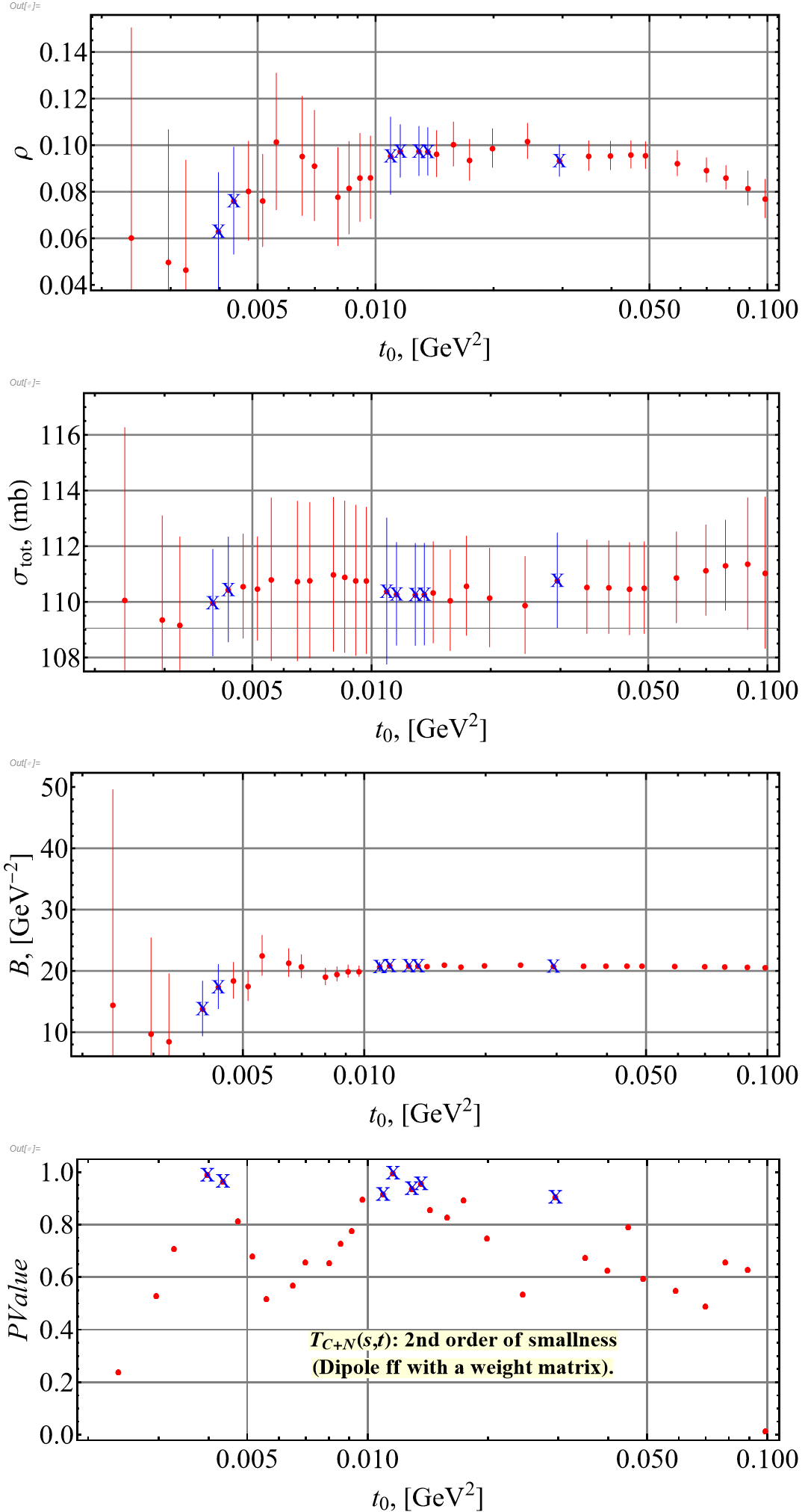
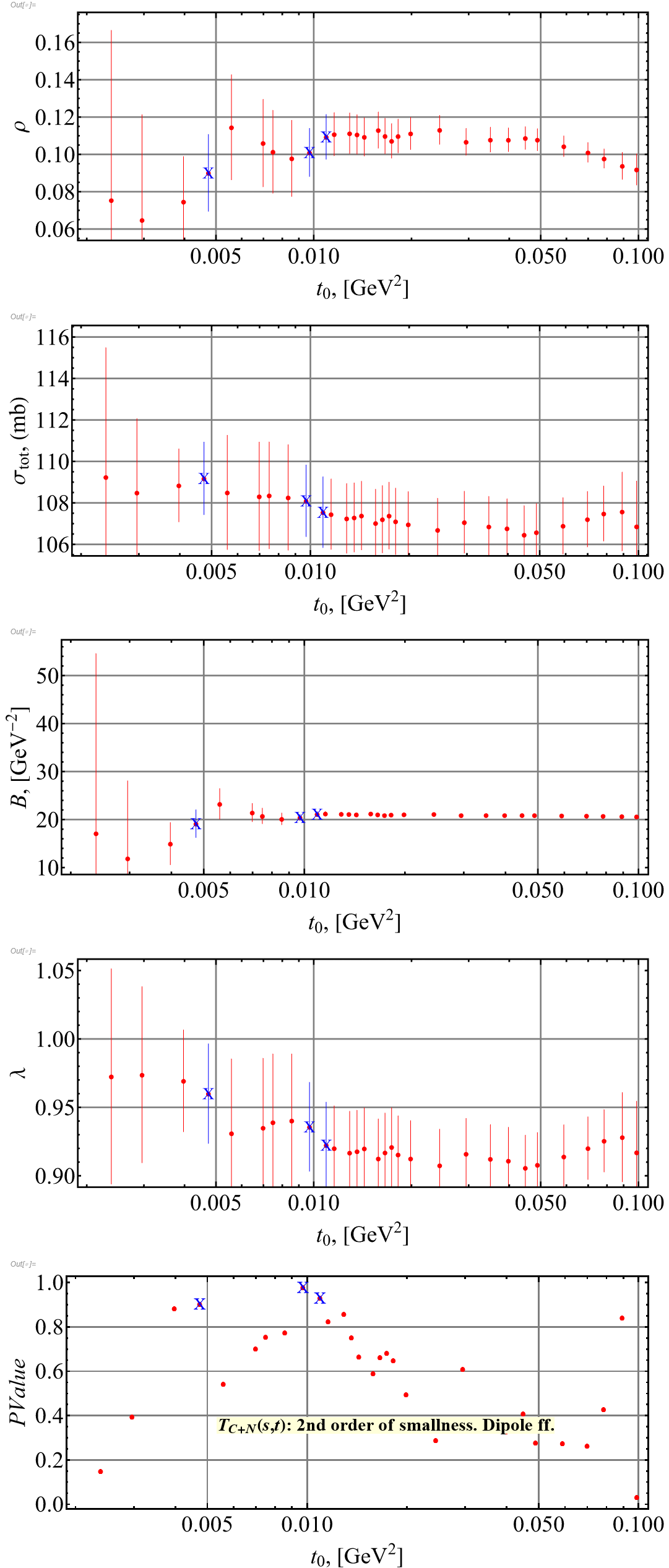
The results are presented in Fig. 1.

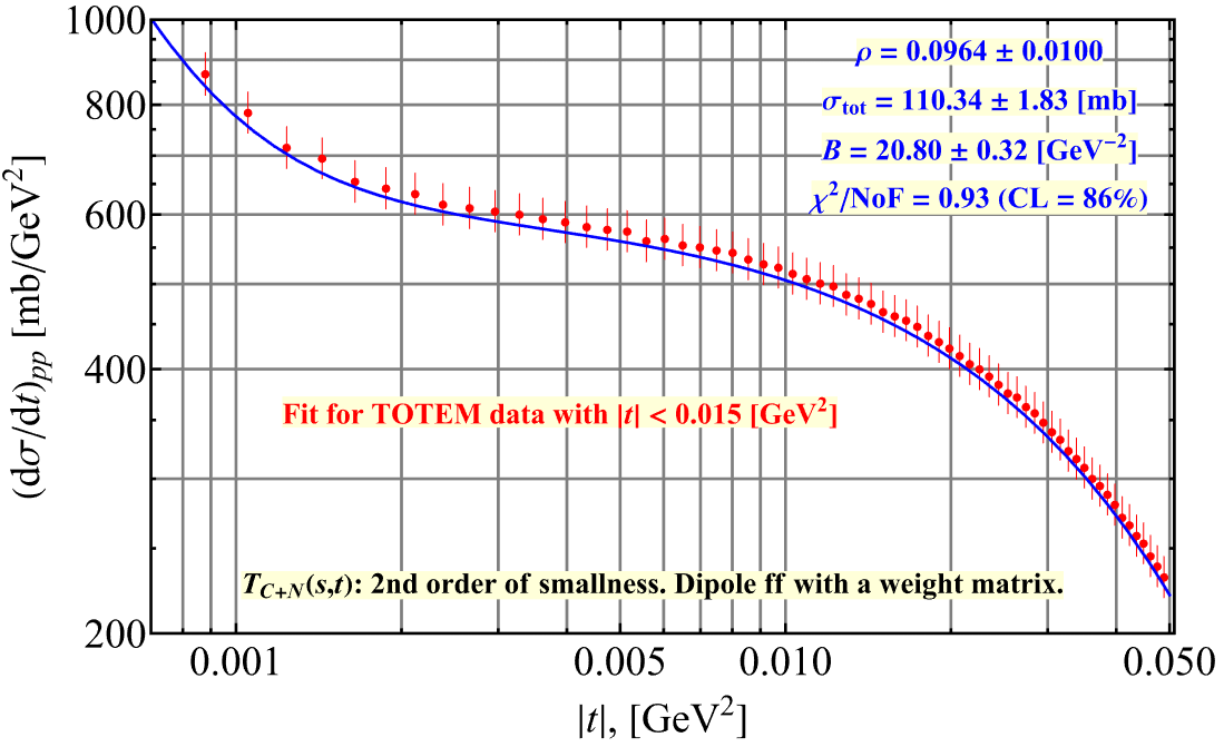
We have analyzed only the fits with p-values $>0.9$ (high level of confidence). One can see in Fig. 1 that the points in the left part of it are unwanted because of their large relative errors. It is seen that in the interval $|t|>0.01\leavevmode\nobreak\ \mbox{GeV}^{2}$ a stabilization of the parameter values occurs and the corresponding values have practically the same and the smallest errors. This is why we dealt with $t_{0}\cong 0.015\leavevmode\nobreak\ \mbox{GeV}^{2}$ which corresponds to the procedure used in our paper [14]. Results of such fitting with corresponding parameters are presented in Fig. 2.

The parameters so retrieved are as follows

$$\rho=0.10\pm 0.01,$$

$$\sigma_{\mbox{tot}}=110.3\pm 1.8\leavevmode\nobreak\ [\mbox{mb}],$$

$$B=20.87\pm 0.35\leavevmode\nobreak\ [\mbox{GeV}^{-2}].$$

However, as is well seen in Fig. 2, the fitting curve for the differential cross-section passes systematically below the average values of experimental points which witnesses that there is an over(under)estimation of the systematic errors.

Figure 2: Results of the fit of the data [1] at $\sqrt{s}=13$ TeV at $|t|\leq t_{0}\cong 0.015\mbox{ GeV}^{2}$. Theoretical curve passes systematically below the experimental values (”PPP effect”). Full errors were obtained using the covariance matrix.

3.2 The $\chi^{2}$-criterion with use of the ”method of the shifting experimental data” (variant 1).

Usually, in the absence of correlations, $\chi^{2}$ is compiled by the formula:

$$\chi^{2}=\sum_{i=1}^{N}\left[\frac{Y^{\mbox{th}}(x_{i})-Y^{\mbox{exp}}(x_{i})}{\sqrt{{\Delta}Y^{2}_{\mbox{stat}}(x_{i})+\Delta Y^{2}_{\mbox{syst}}(x_{i})}}\right]^{2}\vspace{-1.1mm}$$

In the case of correlation this method is not suitable and the function $\chi^{2}$ is compiled using the weight matrix. At the same time, in our case, the experimental data have systematic errors which significantly exceed the statistical error. In this variant, the case is often realized when the value $\chi^{2}/\mbox{NoF}$ turns out to be close to zero, which is statistically unreliable.

If the experimental data allow us to build a weight matrix, then results are often obtained with the final curve systematically passing below or above the experimental points, which is realized in our case considered above.

There is another way to process experimental data when the use of systematic errors allows a shift of the central values of experimental points. There can be many ways to shift the experimental data. Let us consider one of them.

We shift the central values by an amount proportional to the systematic errors and the proportionality coefficient is assumed to be the same and equal to $\lambda$ for all points. $\chi^{2}$ should be written now as:

$$\chi^{2}=\sum_{i=1}^{\infty}\left[\frac{Y^{\mbox{th}}(x_{i})-[Y^{\mbox{exp}}(x_{i})+\lambda\Delta Y_{\mbox{syst}}(x_{i})]}{{\Delta}Y_{\mbox{stat}}(x_{i})}\right]^{2}+\lambda^{2},$$

and the parameter $\lambda$ is the same for all points of the experimental data array. In this particular case, $\lambda^{2}$ is a penalty function for $\chi^{2}$ arising in statistics as a consequence of a shift in the experimental data on systematic errors. I.e. we shift the experimental values up or down by the amount of their systematic errors with a certain factor $\mid\lambda\mid\leq 1$, the same for all experimental points. In this case we leave in the denominator of the expression for $\chi^{2}$ only the statistical error of the measured value. The factor $\lambda$ itself is a fitting parameter.

Fitting in this case should not differ significantly from fitting when used the weight matrix for $\chi^{2}$ and its results (according to Eqs. (7) and (8)) are presented in Fig. 3.

Here we have (see Fig. 3) five points with a very high level of confidence and the more a point lies to the left, the more it satisfies the definition of our basic parameters as given by Eqs.(2).

As above we use only those fits which have p-values $\geq 0.9$. The exact values of the parameters with a high level of confidence (blue dots), taking into account their errors do not allow to give preference to their values for different values of $t_{0}$. Of course, lower values of $t_{0}$ are more preferable, but they have a large error. For large $t_{0}$ the errors are small, but taking them into account reduces compliance with the definitions of the parameters in question as given in Eqs.(2).

Figure 3: Parameter values for different cut-off values of experimental data $t_{0}$. Points with p-value $\geq 0.9$ are marked with crosses.

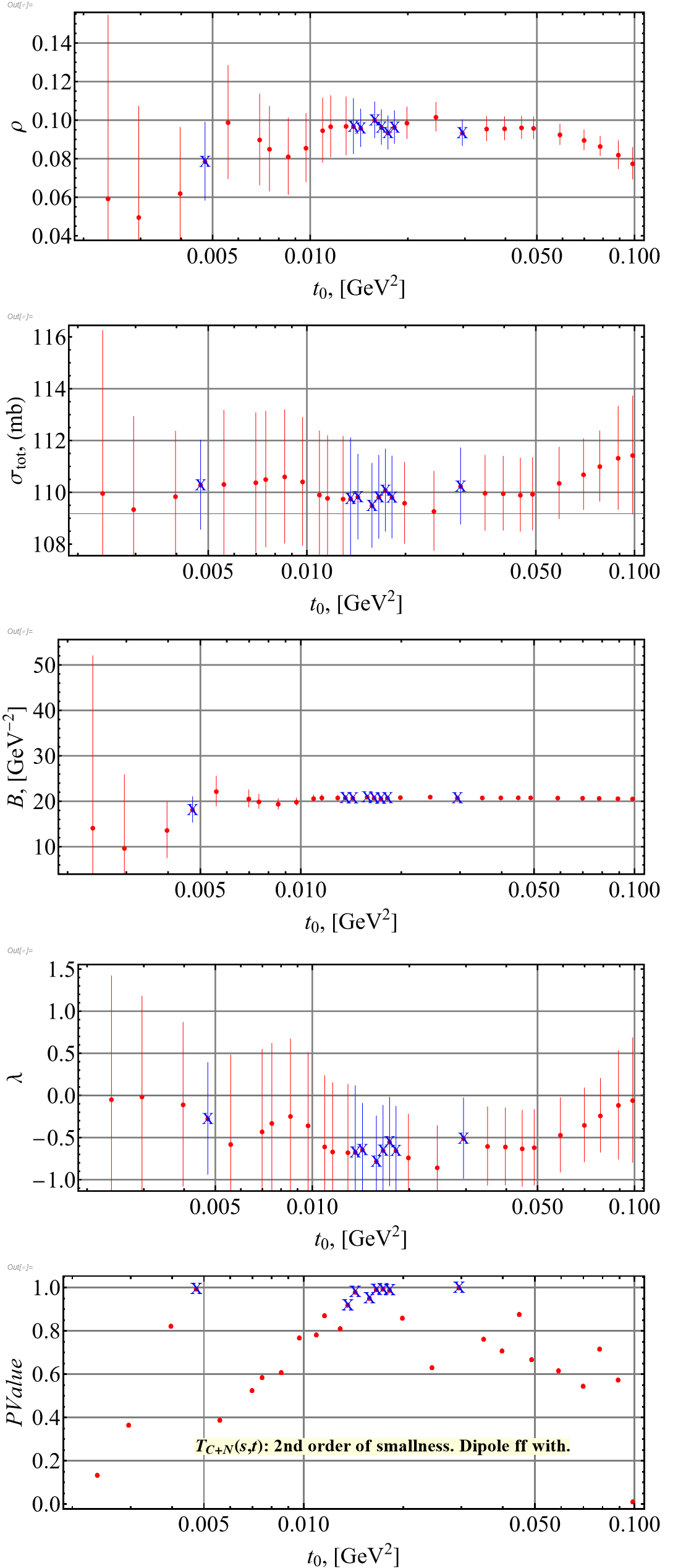
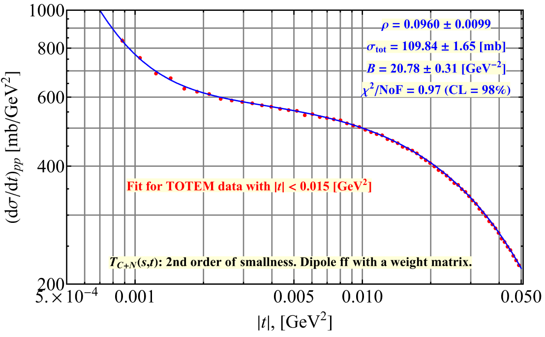
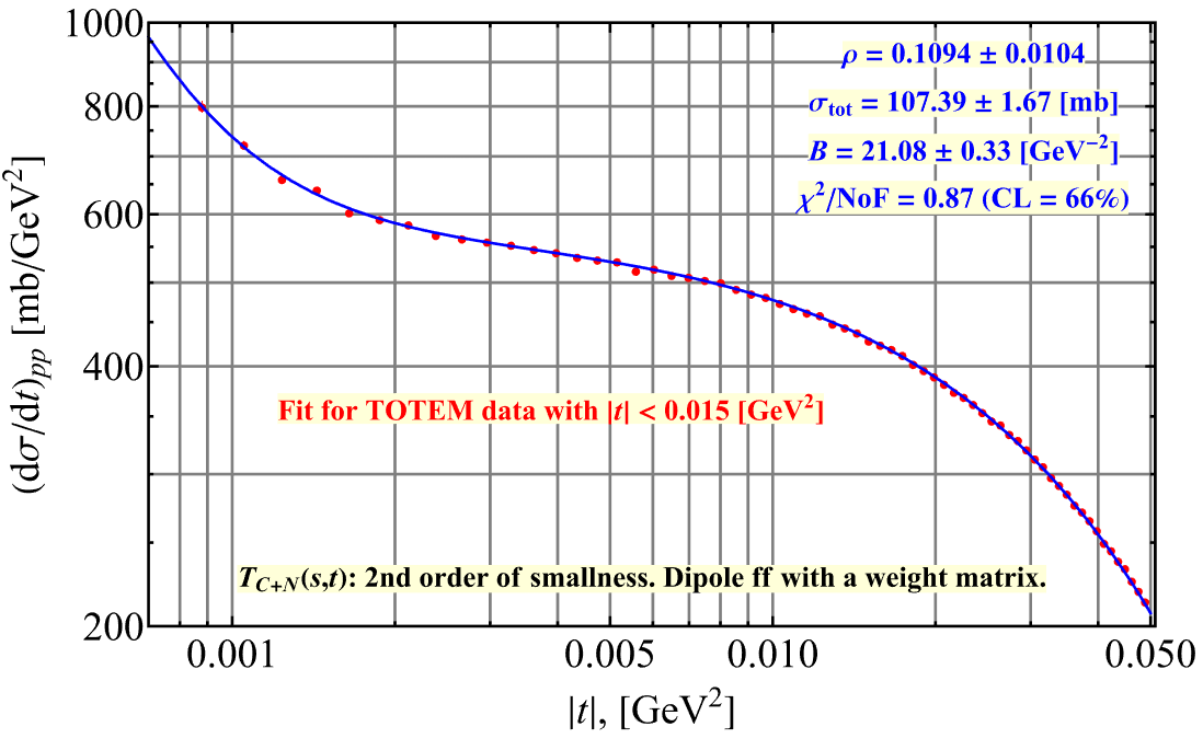
Thus, the values of the parameters, taking into account errors, do not contradict their same values for small and large cut-off values. In the interval $0.01<t_{0}<0.05$, we observe the stability of the parameters extracted from the fitting, and for this reason we use the same method for choosing a particular fit as in the previous case, i.e. we take a fit at $t_{0}\cong 0.015\leavevmode\nobreak\ \mbox{GeV}^{2}$. The results of this fit are shown in Fig. 4.

Extracted parameters are as follows:

$$\rho=0.10\pm 0.01,$$

$$\sigma_{\mbox{tot}}=109.5\pm 1.6\leavevmode\nobreak\ [\mbox{mb}],$$

$$B=21.02\pm 0.26\leavevmode\nobreak\ [\mbox{GeV}^{-2}].$$

We observe a good course of the curve along the experimental points, but already shifted, each by $\lambda=-0.64106$ from its systematic error (downward shift).

Figure 4: Results of fitting the experimental data at $\sqrt{s}=13$ TeV with $|t|<t_{0}\cong 0.015\mbox{ GeV}^{2}$. Only statistical errors are indicated.

3.3 The $\chi^{2}$-criterion with use of the ”method of the shifting experimental data” (variant 2).

Let us consider one more way of shifting the experimental data. We will shift the central values by a value proportional to the (measured) value itself, and the proportionality coefficient $\lambda$ is assumed to be the same for all points. In this case $\chi^{2}$ has in the form

$$\chi^{2}=\sum_{i=1}^{N}\left[\frac{Y^{th}(x_{i})-\lambda Y^{exp}(x_{i})}{{\Delta}Y_{stat}(x_{i})}\right]^{2}+\left(\frac{\lambda-1}{0.055}\right)^{2},$$

and $\lambda$ is the same for all points of the array of experimental data. The second term on the right is a penalty function for $\chi^{2}$, which arises in statistics as a result of an experimental data shift in systematic errors. This form is due to the shifting method and the fact that all systematic errors are equal to $0.055$ of the differential cross section. That is, we shift the experimental values up or down by an amount proportional to the measured value itself. It is clear that in this case $\lambda$ should be positive and close to unity. We assume this factor to be the same for all experimental points. At the same time, in the expression for $\chi^{2}$, we use only the statistical error of the measured value. The multiplier $\lambda$ itself is a fitting parameter.

Fitting in this case should not differ significantly from fitting when using the weight matrix for $\chi^{2}$ and its results are shown in Fig. 5 (according to the formulas in Eq.(7) – (8)).

Here we have only three points with p-value $>0.9.$ So we have no choice but to choose a fit corresponding to the right extreme point with a cross. As before, we observe in the interval $0.01\leavevmode\nobreak\ \mbox{GeV}^{2}<t_{0}<0.05\leavevmode\nobreak\ \mbox{GeV}^{2}$, the stability of the parameters extracted from the fits, and for this reason we use the same method of choosing a specific fit (although in this case we actually have no choice). The results are shown in Fig. 6. The extracted parameters from this fit are as follows:

Figure 5: Parameter values for different cut-off values $t_{0}$. Points with p-value $>0.9$ are marked with crosses.

$$\rho=0.11\pm 0.01,\vspace{-2.1mm}$$

$$\sigma_{\mbox{tot}}=107.6\pm 1.7\>[\mbox{mb}],\vspace{-0.1mm}$$

$$B=21.15\pm 0.55\leavevmode\nobreak\ [\mbox{GeV}^{-2}].\vspace{-0.1mm}$$

One can see a good course of the curve along the experimental points, but already occupying a new central value equal to the coefficient $\lambda=0.920005$ times its old value (central values, as in the previous case, are still moving down).

Thus, we have extracted the values of the parameters in three ways, and all these three sets do not contradict each other (taking into account errors).

However, the values of the $\rho$-parameter do not allow making an unambiguous statement that it is less than 0.1 as in Ref. [1] at $t_{0}=0.07\leavevmode\nobreak\ \mbox{GeV}^{2}$.

Figure 6: Results of the fit of the experimental data at $\sqrt{s}=13\mbox{ TeV}$ and $|t|\lesssim t_{0}=0.015\leavevmode\nobreak\ \mbox{ GeV}^{2}$. Only statistical errors are indicated.

3.4 The last step: cut-off of the experimental data with a small value of $|t|$.

In all the above cases of fitting by the method of cutting off points with a high value of $|t|$, there is a space where the extracted parameters practically do not change. This happens in the interval $0.01\leq|t|\leq 0.05\leavevmode\nobreak\ \mbox{ GeV}^{2}$. However, at $t_{0}<0.01\mbox{ GeV}^{2}$ the values of the extracted parameters experience sharp irregular changes. This is what motivates us to discard the region $|t|<0.01\mbox{ GeV}^{2}$. Of course, the data at $|t|>0.05\mbox{ GeV}^{2}$ should also be discarded, since above this limit the extracted parameters begin to experience noticeable changes and the confidence level becomes unacceptably low.

Thus, we use only experimental data for which the stability of the extracted parameters was observed above, i.e. the interval

$$0.01\mbox{ GeV}^{2}\lesssim|t|\lesssim 0.05\mbox{ GeV}^{2}.$$

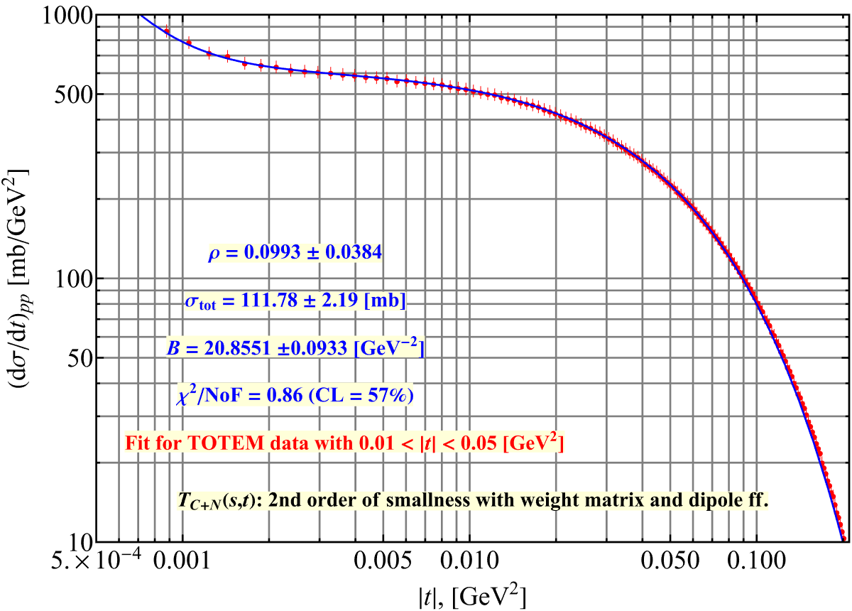
The results of the fit of these data using the weight matrix are shown in Fig. 7.

Figure 7: The summary of parameters.The number of decimal places to retain in parameter values is given according to the arguments in [17].

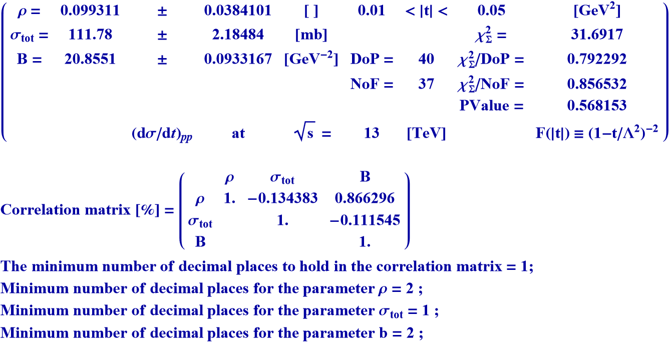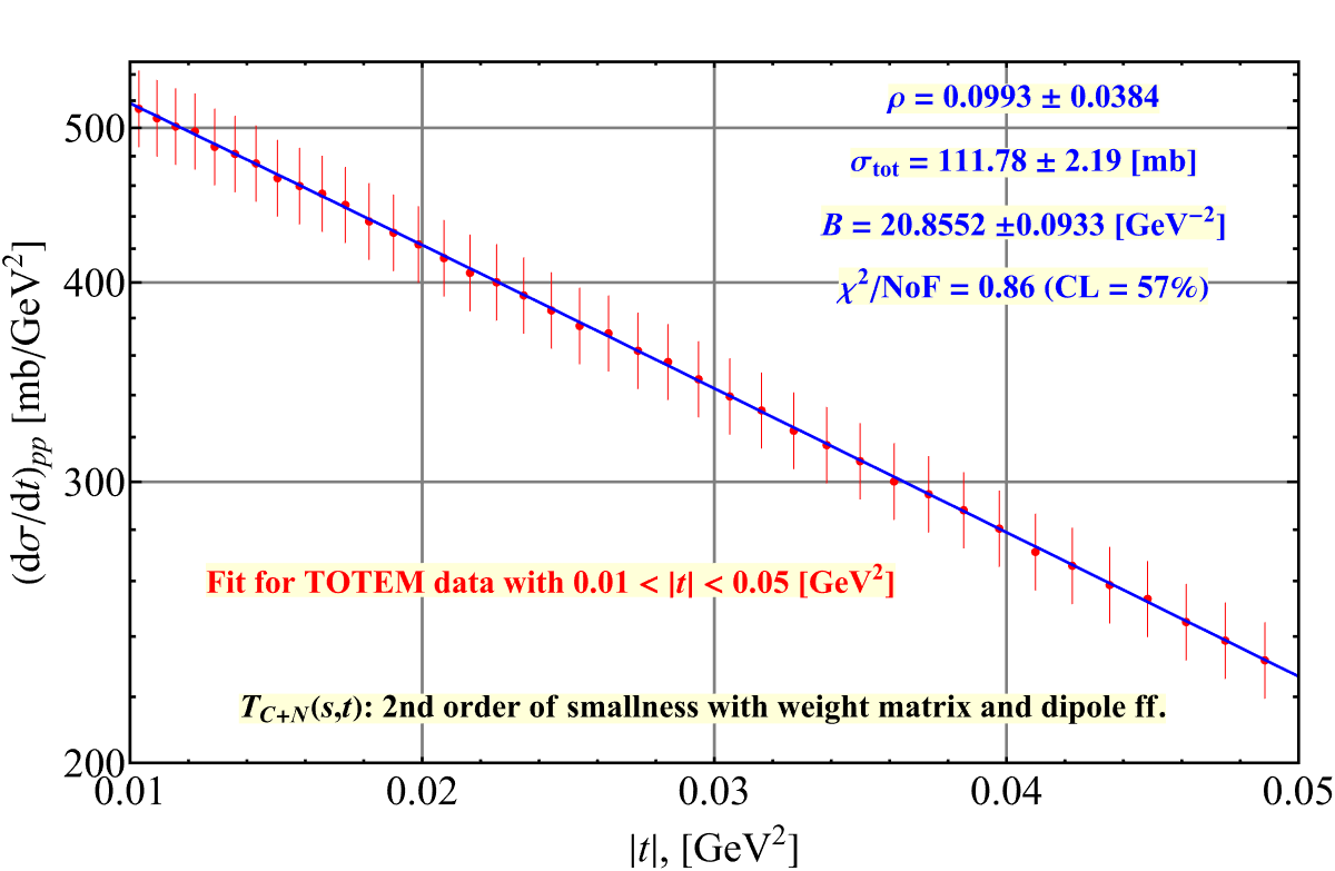
In Fig. 8 it can be seen that the theoretical curve and the experimental data are in perfect agreement. Apparently, this result is the most reliable on the TOTEM experimental data array at $\sqrt{s}=13$ TeV.

For completeness, we present in Fig. 9 the behaviour of the descriptive curve on the entire array of experimental data.

Figure 8: Results of experimental data fitting on the interval $0.01\leq|t|\leq 0.05\mbox{ GeV}^{2}$ with use of the weight matrix. The scale along the vertical axis is logarithmic. The total errors extracted from the weight matrix are indicated. It can be seen that in this case there is no regular shift of the theoretical curve relative to the central experimental points, in contrast to the fitting on the full array (with a weight matrix).

Figure 9: Theoretical description of the full TOTEM data on $(d\sigma/dt)_{pp}$ at $\sqrt{s}=13$ TeV. The fit was carried out on the interval $0.01\lesssim|t|\lesssim 0.05\mbox{ GeV}^{2}$.

The above fittings in two different ways with a shift in experimental data give excellent statistical results and both indicate the possible fact of overestimated central values of the experimental data of differential cross sections. This is consistent with the first fitting result we cited above, where the theoretical curve systematically passes below the central values.

Such a picture is nothing but a manifestation of the properties of the weight matrix given by the TOTEM group. It is possible to get rid of this contradictory picture of the need to correct the experimental data (which, in our opinion, is an unacceptable operation) only by limiting the TOTEM experimental data sample to the segment $0.01\lesssim|t|\lesssim 0.05\mbox{ GeV}^{2}$. This leads to a new, different from the TOTEM, value of the $\rho$-parameter and, most importantly, to its larger error ($\approx 40\%$), which makes the results obtained in this way quite compatible with the results of the COMPETE collaboration.

Thus, we carried out three types of processing of experimental TOTEM data, described above by the method of a step-by-step exclusion of experimental data with high values of $q^{2}$. In all these methods, approximately the same parameter values were obtained (see above), roughly near the values of the TOTEM group. A common property of these three methods is the fact that they exhibit a high degree of parameter stabilization when using experimental data for which $q^{2}\leq 0.05GeV^{2}$, and with a high degree of confidence - more than $85\%$. However, all three of these methods have significant drawbacks. In the first method, the theoretical curve systematically passes below the experimental values, while in the second and third methods, it is generally necessary to shift the experimental values, and these methods, although they perfectly describe the shifted experimental values, do not use the correlation (weight) matrix given by the experimenters.

The most significant drawback of these three methods is the fact that when discarding experimental points with a high $q^{2}$ - value ($q^{2}\gtrsim 0.05\mbox{ GeV}^{2}$), there is, in the area of $q^{2}\lesssim 0.01\mbox{ GeV}^{2}$, a significant decrease in the confidence level of the obtained parameter values and their significant change in [central] values (especially the parameter $\rho$) with a simultaneous sharp increase retrieved parameter errors.

This prompted us, when processing the experimental values, to discard not only the experimental data for which $q^{2}\leq 0.05GeV^{2}$, but also those for which $q^{2}\leq 0.01GeV^{2}$. Of course, we used the correlation matrix (weight matrix) in this case. In this case, the results are obtained with a high level of confidence and without the shortcomings that we mentioned above. They are shown in Fig. 9.

However, the price of getting rid of all the shortcomings of extracting experimental data was a high error for the value of the $\rho$ - parameter, which reaches about $40\%$. However, the theoretical curve does not systematically pass above or below the experimental points (see Figures 8 and 9), and the confidence level turns out to be even higher than $50\%$ .

For this reason, we consider these parameter values to be the most consistent with the experimental measurements of the TOTEM group.

Separately, we investigated the influence of the dipole form factor, which we used everywhere above, on the results obtained. To do this, we carried out similar calculations using the exact formulas for the unit form factor (”electrically point like protons”). The results turned out to be practically indistinguishable from the above values of the parameters for the dipole form factor. From this we conclude that the use of the $\mathcal{O}(\alpha^{2})$-approximation for the description of the differential cross-section is quite sufficient at the range of the transferred momenta considered.

Conclusions and outlook

In the present paper, a comprehensive discussion of various methods for extracting the $\rho$ parameter from the experimental results of the TOTEM collaboration at $\sqrt{s}=13$ TeV has been carried out.

Theoretically substantiated formulas, Eqs.(4) – (5) and, for a certain general form for $T_{N}$ (Eq. 6), Eqs. (7) – (8), are derived which allow us to describe the data for small values of $q^{2}$ ($|t|$) .

It is shown that in order to extract the $\rho$ parameter from the experimental data [1] in a statistically sound manner, one can account only for points that satisfy the condition $0.01\lesssim|t|\lesssim 0.05\leavevmode\nobreak\ \mbox{GeV}^{2}$. Consequently, although the value of $\rho$ remains to be close to 0.1, its root-mean-square error increases, in contrast with the TOTEM result (10%), to almost 40%.

For this reason, we consider it premature to conclude, as the authors of many papers did, that the value of the $\rho$ parameter was determined by the TOTEM collaboration at $\sqrt{s}=13$ TeV very accurately, with $\rho=0.09\pm 0.01$ (from the array with $|t|\leq 0.07\leavevmode\nobreak\ \mbox{GeV}^{2}$).

It is also premature to draw far-reaching physical conclusions based on these measurements, such as the existence of an Odderon or, at least, its significant contribution to the forward observables.

The aforesaid gives us also a reason to consider the conclusion about the failure of the COMPETE predictions [3] announced in [1] to be unfounded.

Below we give the summary of the concrete numerical values of the basic parameters obtained in this paper.

I

With use of the IR regular expression (7) – (8) for the differential cross-section $d\sigma^{\leavevmode\nobreak\ pp}_{C+N}/dt$ which accounts in a correct way (in the $\mathcal{O}(\alpha^{2})$ approximation) for the Coulombic contribution we have retrieved from the TOTEM data [1] the following values of three important parameters at $\sqrt{s}=13$ TeV:

$$\sigma_{\mbox{tot}}^{\leavevmode\nobreak\ pp}=111.8\pm 2.2\mbox{ mb},$$ (9)

$$B^{\leavevmode\nobreak\ pp}=20.86\pm 0.09\mbox{ GeV}^{-2},$$

$$\rho=0.10\pm 0.04,$$

$$0.01\lesssim|t|\lesssim 0.05\mbox{ GeV}^{2}.$$

II

In order to check the influence of the smearing of the electric charge over the proton volume we have considered the idealized case of ”electrically point-like protons” ($\mathcal{F}=1$)and have retrieved the following result:

$$\sigma_{\mbox{tot}}^{\leavevmode\nobreak\ pp}=111.8\pm 2.2\mbox{ mb},$$ (10)

$$B^{\leavevmode\nobreak\ pp}=20.86\pm 0.09\mbox{ GeV}^{-2},$$

$$\rho=0.10\pm 0.04,$$

$$0.01\lesssim|t|\lesssim 0.05\mbox{ GeV}^{2}.$$

It practically coincides with Eq. (9). What could mean a coincidence of two sets (9) and (10)?

The spread of the electric charge inside the proton is limited by the physical size of the proton (of its valence core responsible for the form factor at small $t$) which amounts to (in the transverse projection) about 0.6 fm [18] . The transverse interaction region is $(2B)^{1/2}$. At $\sqrt{s}=13$ TeV the average size of the interaction region is about 1.3 fm . According to such a reasoning the proper size of the proton can be hardly neglected in comparison with the average interaction radius. So the mentioned coincidence seems a little puzzle. Although one could argue that the form factors are essentially close to $1$ at considered $t$. However, the form factors enter also the integrals in Eq.(5).

III

Now we are to compare our results (9) with the published values [1] retrieved on the basis of a different theoretical requisite [9] to treat CNI:

$$\sigma_{\mbox{tot}}^{pp}=110.5\pm 2.4\mbox{ mb},$$ (11)

$$B^{pp}=21.78\pm 0.06\mbox{ GeV}^{-2},$$

$$\rho=0.09\pm 0.01,$$

$$|t|\leq 0.07\mbox{ GeV}^{2}.$$

Note that the parameters $\sigma_{\mbox{tot}}^{pp}$ and $b^{pp}$ of both sets differ little ( $\leq 1\%$ )both in central values and in errors. However, the values of $\rho^{pp}$ differ quite a lot. The difference is $10\%$ for the central value and $30\%$ for the error band.

At first sight, our result Eq. (9) looks quite ordinarily being, in terms of $\rho$, close to the TOTEM result Eq. (11) (although such a difference may have a significant physical reason). However, a conceptually important point is that such a widening of the error corridor in Eq.(9) in compare with Eq. (11) ”returns to the agenda” a number of models (giving $0.12\leq\rho\leq 0.14$, see e.g.[19])which are to be rejected according to [1] .

Let us remind that in this paper we used in capacity of the nuclear amplitude $T_{N}$ the option (6) which, though widely used in literature (including the TOTEM publication [1]) , is, strictly speaking, not fully satisfactory because of $t$ -independence of its phase.

We have also to notice that the values of $\rho$ retrieved with help of different models of $T_{N}$ are inevitably different. Such a semi-theoretical character of the $\rho$-parameter was realized for a long time but never studied systematically.

We hope to further investigate these important issues in forthcoming studies.

Appendix A. On the difference between the $\alpha$-expansions of the exact expression for $d\sigma_{C+N}/dt$ and the CKL approximation.

As was already mentioned above, the CKL scheme shows two flaws.

To begin with, the account of the form factor in the formula for the full amplitude $T_{C+N}$ was assumed in a simplified way, different from the exact account. Moreover, when using the expansion in $\alpha$ CKL [9] retain in the $T_{C+N}$ only the first order term. Since this approximation is then used in $\mid T_{C+N}\mid^{2}\sim d\sigma_{C+N}/dt$ one must either use only the $\mathcal{O}(\alpha)$-approximation also in $d\sigma_{C+N}/dt$ (which would eventually lead to an absurd situation) or, to be mathematically correct, keep the $\mathcal{O}(\alpha^{2})$-term already in the amplitude. Otherwise, there is a missing $\mathcal{O}(\alpha^{2})$ - term in $d\sigma_{C+N}/dt$.

It is not difficult to retain the $\mathcal{O}(\alpha^{2})$ - term in the $\alpha$ -expansion of $T_{C+N}^{CKL}$ (ignoring the aforesaid blunder with account of the form factor)and this is what we have done in order to make the comparison between the two schemes better reflecting the essence of the matter. Thus modified CKL cross-section (i.e. corrected with retaining of the $\alpha^{2}$ term in the full amplitude) differs from the $\alpha$ -expansion of the exact expression (4), (5) by a decrement

$$\delta\left[\frac{d\sigma_{C+N}}{dt}\right]\equiv\frac{d\sigma_{C+N}}{dt}-\frac{d\sigma^{CKL}_{C+N}}{dt}$$

which takes place in the second order in $\alpha$ only and reads as follows

$$\delta\left[\frac{d\sigma_{C+N}}{dt}\right]=(\hbar c)^{2}\frac{\alpha^{2}}{2\pi sq^{2}}\int\frac{dk^{2}}{k^{2}}\frac{dp^{2}}{p^{2}}(-\lambda(q^{2},k^{2},p^{2}))_{+}^{-1/2}\cdot\leavevmode\nobreak\ \leavevmode\nobreak\ \leavevmode\nobreak\ \leavevmode\nobreak\ \leavevmode\nobreak\ \leavevmode\nobreak\ \leavevmode\nobreak\ \leavevmode\nobreak\ \leavevmode\nobreak\ \leavevmode\nobreak\ \leavevmode\nobreak\ \leavevmode\nobreak\ \leavevmode\nobreak\ \leavevmode\nobreak\ \leavevmode\nobreak\ \leavevmode\nobreak\ \leavevmode\nobreak\ \leavevmode\nobreak\ \leavevmode\nobreak\ \leavevmode\nobreak\ \leavevmode\nobreak\ \leavevmode\nobreak\ \leavevmode\nobreak\ \leavevmode\nobreak\ \leavevmode\nobreak\ \leavevmode\nobreak\ \leavevmode\nobreak\ \leavevmode\nobreak\ \leavevmode\nobreak\ \leavevmode\nobreak\ \leavevmode\nobreak\ \leavevmode\nobreak\ \leavevmode\nobreak\ \leavevmode\nobreak\ \leavevmode\nobreak\ \leavevmode\nobreak\ \leavevmode\nobreak\ \leavevmode\nobreak\ \leavevmode\nobreak\ \leavevmode\nobreak\ \leavevmode\nobreak\ \leavevmode\nobreak\ \leavevmode\nobreak\ \leavevmode\nobreak\ \leavevmode\nobreak\ \leavevmode\nobreak\ \leavevmode\nobreak\ \leavevmode\nobreak\ \leavevmode\nobreak\ \leavevmode\nobreak\ \leavevmode\nobreak\ \leavevmode\nobreak\ \leavevmode\nobreak\ \leavevmode\nobreak\ \leavevmode\nobreak\ \leavevmode\nobreak\ \leavevmode\nobreak\ \leavevmode\nobreak\ \leavevmode\nobreak\ \leavevmode\nobreak\ \leavevmode\nobreak\ \leavevmode\nobreak\ \leavevmode\nobreak\ \leavevmode\nobreak\ \leavevmode\nobreak\ \leavevmode\nobreak\$$

$$\leavevmode\nobreak\ \leavevmode\nobreak\ \leavevmode\nobreak\ \leavevmode\nobreak\ \leavevmode\nobreak\ \leavevmode\nobreak\ \leavevmode\nobreak\ \leavevmode\nobreak\ \leavevmode\nobreak\ \leavevmode\nobreak\ \leavevmode\nobreak\ \leavevmode\nobreak\ \leavevmode\nobreak\ \leavevmode\nobreak\ \leavevmode\nobreak\ \leavevmode\nobreak\ \leavevmode\nobreak\ \leavevmode\nobreak\ \leavevmode\nobreak\ \leavevmode\nobreak\ \leavevmode\nobreak\ \leavevmode\nobreak\ \cdot\left\{q^{2}\mbox{Im}T_{N}(q^{2})\left[\mathcal{F}^{2}(k^{2})\mathcal{F}^{2}(p^{2})-\mathcal{F}^{2}(q^{2})\right]-k^{2}\mbox{Im}T_{N}(k^{2})\left[\mathcal{F}^{2}(p^{2})\mathcal{F}^{2}(q^{2})-\mathcal{F}^{2}(k^{2})\right]-\right.$$

$$\leavevmode\nobreak\ \leavevmode\nobreak\ \leavevmode\nobreak\ \leavevmode\nobreak\ \leavevmode\nobreak\ \leavevmode\nobreak\ \leavevmode\nobreak\ \leavevmode\nobreak\ \leavevmode\nobreak\ \leavevmode\nobreak\ \leavevmode\nobreak\ \leavevmode\nobreak\ \leavevmode\nobreak\ \leavevmode\nobreak\ \leavevmode\nobreak\ \leavevmode\nobreak\ \leavevmode\nobreak\ \leavevmode\nobreak\ \leavevmode\nobreak\ \leavevmode\nobreak\ \leavevmode\nobreak\ \leavevmode\nobreak\ \leavevmode\nobreak\ \leavevmode\nobreak\ \leavevmode\nobreak\ \leavevmode\nobreak\ \leavevmode\nobreak\ \leavevmode\nobreak\ \leavevmode\nobreak\ \leavevmode\nobreak\ \leavevmode\nobreak\ \leavevmode\nobreak\ \leavevmode\nobreak\ \leavevmode\nobreak\ \leavevmode\nobreak\ \leavevmode\nobreak\ \leavevmode\nobreak\ \leavevmode\nobreak\ \leavevmode\nobreak\ \leavevmode\nobreak\ \leavevmode\nobreak\ \leavevmode\nobreak\ \leavevmode\nobreak\ \leavevmode\nobreak\ \leavevmode\nobreak\ \leavevmode\nobreak\ \leavevmode\nobreak\ \leavevmode\nobreak\ \leavevmode\nobreak\ \leavevmode\nobreak\ \leavevmode\nobreak\ \leavevmode\nobreak\ \leavevmode\nobreak\ \leavevmode\nobreak\ \leavevmode\nobreak\ \leavevmode\nobreak\ \leavevmode\nobreak\ \leavevmode\nobreak\ \leavevmode\nobreak\ \leavevmode\nobreak\ \leavevmode\nobreak\ \leavevmode\nobreak\ \leavevmode\nobreak\ \leavevmode\nobreak\ \leavevmode\nobreak\ \leavevmode\nobreak\ \leavevmode\nobreak\ \leavevmode\nobreak\ \leavevmode\nobreak\ \leavevmode\nobreak\ \leavevmode\nobreak\ \leavevmode\nobreak\ \leavevmode\nobreak\ \leavevmode\nobreak\ \leavevmode\nobreak\ \leavevmode\nobreak\ \leavevmode\nobreak\ \left.-p^{2}\mbox{Im}T_{N}(p^{2})\left[\mathcal{F}^{2}(q^{2})\mathcal{F}^{2}(k^{2})-\mathcal{F}^{2}(p^{2})\right]\right\}+$$

$$\leavevmode\nobreak\ \leavevmode\nobreak\ \leavevmode\nobreak\ \leavevmode\nobreak\ \leavevmode\nobreak\ \leavevmode\nobreak\ \leavevmode\nobreak\ \leavevmode\nobreak\ \leavevmode\nobreak\ \leavevmode\nobreak\ \leavevmode\nobreak\ \leavevmode\nobreak\ \leavevmode\nobreak\ \leavevmode\nobreak\ \leavevmode\nobreak\ \leavevmode\nobreak\ \leavevmode\nobreak\ +\frac{\alpha^{2}}{4\pi(\hbar c)^{2}s^{2}(2\pi)^{2}}\int\frac{d^{2}k}{k^{2}}\frac{d^{2}p}{p^{2}}\left[\mathcal{F}^{2}\left((k+p)^{2}\right)-\mathcal{F}^{2}(k^{2})\mathcal{F}^{2}(p^{2})\right]\cdot\mbox{Re}\left[T_{N}(q^{2})T^{*}_{N}\left((q-k-p)^{2}\right)\right]$$

In the point like limit $\mathcal{F}\rightarrow 1$, the above integrals turn out to be equal to zero and the CKL approximation (adjusted for the $\alpha^{2}$-term retention in the amplitude) is equivalent to our formulas.

The decrement would also be equal to zero if the amplitude in $T_{C+N}^{CKL}$ differed from $T_{C+N}$ only by a phase factor. In this case, the amplitudes would be physically equivalent. However, as we see, this is not the case.

In general case the decrement behaves at small $q^{2}$ as

$$\delta\left[\frac{d\sigma_{C+N}}{dt}\right]\approx-\frac{\alpha^{2}}{16\pi}\left\{\left[\ln\left(\frac{\Lambda^{2}}{q^{2}}\right)-\frac{11}{6}-A\left(\frac{B\Lambda^{2}}{2}\right)\right]^{2}\frac{\sigma^{2}_{\mbox{tot}}}{(\hbar c)^{2}}+64\pi\mathcal{F}^{2}(q^{2})\frac{\sigma_{\mbox{tot}}}{\Lambda^{2}}\right\}$$

where

$$A(z)=\int_{0}^{\infty}\frac{(1-e^{-zx})}{x(1+x)^{4}}dx=\mathcal{C}+\frac{z^{2}-4z+\mbox{Ei}(-z)e^{z}(z^{3}-3z^{2}+6z-6)}{6}+\ln z.$$

In his talk at the Low-x 2021 Workshop at Elba [22] K.Österberg had presented the comparison of our approach (as explained most recently in [13]) with the CKL approximate scheme [9]( adopted in [1]) with a severe sentence(basing on the paper [23]):

”the new CNI formula from Petrov… fails”.

Actually the comparison was made not in terms of the ratio $d\sigma_{C+N}/d\sigma_{C+N}^{CKL}$ but, instead, of the ratio $d\sigma_{C+N}^{1}/d\sigma_{C+N}^{CKL}$ where $d\sigma_{C+N}^{1}/dt$ is the cross-section with only the first-order contribution in $\alpha$ in the full amplitude and which was called the ”new CNI formula from Petrov” in spite of that we specially emphasized the role of the second order in [13].

The ratio $d\sigma_{C+N}^{1}/d\sigma_{C+N}^{CKL}$ showed a ($4\%$) deviation from unity (in the region of low t) which was misunderstandingly qualified as a failure of our approach [12], [13].

To clear things up let us, in our turn, estimate the comparative quality of the quantity $d\sigma_{C+N}^{1}/dt$ and the TOTEM working tool, the CKL expression $d\sigma_{C+N}^{CKL}/dt$ [1], [9]. At Fig. 10 we show (similar to what was done in [23]) the ratios $(d\sigma/dt-ref)/ref$ where we assume as a reference value, $ref$, our expression in Eq. (7) while for $d\sigma/dt$ we take $d\sigma_{C+N}^{CKL}/dt$ and $d\sigma_{C+N}^{1}/dt$. :

$$\mbox{Ratio 1}=d\sigma_{C+N}^{CKL}/d\sigma_{C+N}-1=\leavevmode\nobreak\ \leavevmode\nobreak\ \leavevmode\nobreak\ \leavevmode\nobreak\ \leavevmode\nobreak\ \leavevmode\nobreak\ \leavevmode\nobreak\ \leavevmode\nobreak\ \leavevmode\nobreak\ \leavevmode\nobreak\ \leavevmode\nobreak\ \leavevmode\nobreak\ \leavevmode\nobreak\ \leavevmode\nobreak\ \leavevmode\nobreak\ \leavevmode\nobreak\ \leavevmode\nobreak\ \leavevmode\nobreak\ \leavevmode\nobreak\ \leavevmode\nobreak\ \leavevmode\nobreak\ \leavevmode\nobreak\ \leavevmode\nobreak\ \leavevmode\nobreak\ \leavevmode\nobreak\ \leavevmode\nobreak\ \leavevmode\nobreak\ \leavevmode\nobreak\ \leavevmode\nobreak\ \leavevmode\nobreak\ \leavevmode\nobreak\ \leavevmode\nobreak\ \leavevmode\nobreak\ \leavevmode\nobreak\ \leavevmode\nobreak\ \leavevmode\nobreak\ \leavevmode\nobreak\ \leavevmode\nobreak\ \leavevmode\nobreak\ \leavevmode\nobreak\ \leavevmode\nobreak\ \leavevmode\nobreak\ \leavevmode\nobreak\ \leavevmode\nobreak\ \leavevmode\nobreak\ \leavevmode\nobreak\ \leavevmode\nobreak\ \leavevmode\nobreak\ \leavevmode\nobreak\ \leavevmode\nobreak\ \leavevmode\nobreak\ \leavevmode\nobreak\ \leavevmode\nobreak\ \leavevmode\nobreak\ \leavevmode\nobreak\ \leavevmode\nobreak\ \leavevmode\nobreak\ \leavevmode\nobreak\ \leavevmode\nobreak\ \leavevmode\nobreak\ \leavevmode\nobreak\ \leavevmode\nobreak\ \leavevmode\nobreak\ \leavevmode\nobreak\ \leavevmode\nobreak\ \leavevmode\nobreak\ \leavevmode\nobreak\ \leavevmode\nobreak\ \leavevmode\nobreak\ \leavevmode\nobreak\ \leavevmode\nobreak\ \leavevmode\nobreak\ \leavevmode\nobreak\ \leavevmode\nobreak\ \leavevmode\nobreak\ \leavevmode\nobreak\ \leavevmode\nobreak\ \leavevmode\nobreak\ \leavevmode\nobreak\ \leavevmode\nobreak\ \leavevmode\nobreak\ \leavevmode\nobreak\ \leavevmode\nobreak\ \leavevmode\nobreak\ \leavevmode\nobreak\ \leavevmode\nobreak\ \leavevmode\nobreak\ \leavevmode\nobreak\ \leavevmode\nobreak\ \leavevmode\nobreak\ \leavevmode\nobreak\ \leavevmode\nobreak\ \leavevmode\nobreak\ \leavevmode\nobreak\ \leavevmode\nobreak\ \leavevmode\nobreak\ \leavevmode\nobreak\$$

$$\leavevmode\nobreak\ \leavevmode\nobreak\ \leavevmode\nobreak\ =\alpha^{2}\left\{\frac{\sigma^{2}_{\mbox{tot}}e^{-Bq^{2}}\left[A(B\lambda^{2}/2)-\ln(\Lambda^{2}/q^{2})+11/6\right]^{2}}{16\pi(\hbar c)^{2}}+\frac{4\mathcal{F}^{2}(q^{2})\sigma_{\mbox{tot}}\ln(1+q^{2}/\Lambda^{2})e^{-Bq^{2}/2}}{q^{2}}\right\}/\left(\frac{d\sigma_{C+N}}{dt}\right)$$

$$\mbox{Ratio 2}=d\sigma_{C+N}^{1}/d\sigma_{C+N}-1=\leavevmode\nobreak\ \leavevmode\nobreak\ \leavevmode\nobreak\ \leavevmode\nobreak\ \leavevmode\nobreak\ \leavevmode\nobreak\ \leavevmode\nobreak\ \leavevmode\nobreak\ \leavevmode\nobreak\ \leavevmode\nobreak\ \leavevmode\nobreak\ \leavevmode\nobreak\ \leavevmode\nobreak\ \leavevmode\nobreak\ \leavevmode\nobreak\ \leavevmode\nobreak\ \leavevmode\nobreak\ \leavevmode\nobreak\ \leavevmode\nobreak\ \leavevmode\nobreak\ \leavevmode\nobreak\ \leavevmode\nobreak\ \leavevmode\nobreak\ \leavevmode\nobreak\ \leavevmode\nobreak\ \leavevmode\nobreak\ \leavevmode\nobreak\ \leavevmode\nobreak\ \leavevmode\nobreak\ \leavevmode\nobreak\ \leavevmode\nobreak\ \leavevmode\nobreak\ \leavevmode\nobreak\ \leavevmode\nobreak\ \leavevmode\nobreak\ \leavevmode\nobreak\ \leavevmode\nobreak\ \leavevmode\nobreak\ \leavevmode\nobreak\ \leavevmode\nobreak\ \leavevmode\nobreak\ \leavevmode\nobreak\ \leavevmode\nobreak\ \leavevmode\nobreak\ \leavevmode\nobreak\ \leavevmode\nobreak\ \leavevmode\nobreak\ \leavevmode\nobreak\ \leavevmode\nobreak\ \leavevmode\nobreak\ \leavevmode\nobreak\ \leavevmode\nobreak\ \leavevmode\nobreak\ \leavevmode\nobreak\ \leavevmode\nobreak\ \leavevmode\nobreak\ \leavevmode\nobreak\ \leavevmode\nobreak\ \leavevmode\nobreak\ \leavevmode\nobreak\ \leavevmode\nobreak\ \leavevmode\nobreak\ \leavevmode\nobreak\ \leavevmode\nobreak\ \leavevmode\nobreak\ \leavevmode\nobreak\ \leavevmode\nobreak\ \leavevmode\nobreak\ \leavevmode\nobreak\ \leavevmode\nobreak\ \leavevmode\nobreak\ \leavevmode\nobreak\ \leavevmode\nobreak\ \leavevmode\nobreak\ \leavevmode\nobreak\ \leavevmode\nobreak\ \leavevmode\nobreak\ \leavevmode\nobreak\ \leavevmode\nobreak\ \leavevmode\nobreak\ \leavevmode\nobreak\ \leavevmode\nobreak\ \leavevmode\nobreak\ \leavevmode\nobreak\ \leavevmode\nobreak\ \leavevmode\nobreak\ \leavevmode\nobreak\ \leavevmode\nobreak\ \leavevmode\nobreak\ \leavevmode\nobreak\ \leavevmode\nobreak\ \leavevmode\nobreak\ \leavevmode\nobreak\ \leavevmode\nobreak\ \leavevmode\nobreak\ \leavevmode\nobreak\$$

$$\leavevmode\nobreak\ \leavevmode\nobreak\ \leavevmode\nobreak\ \leavevmode\nobreak\ \leavevmode\nobreak\ \leavevmode\nobreak\ \leavevmode\nobreak\ \leavevmode\nobreak\ \leavevmode\nobreak\ \leavevmode\nobreak\ \leavevmode\nobreak\ \leavevmode\nobreak\ \leavevmode\nobreak\ \leavevmode\nobreak\ \leavevmode\nobreak\ \leavevmode\nobreak\ \leavevmode\nobreak\ \leavevmode\nobreak\ \leavevmode\nobreak\ \leavevmode\nobreak\ \leavevmode\nobreak\ \leavevmode\nobreak\ \leavevmode\nobreak\ =\alpha^{2}\left\{\frac{\sigma_{\mbox{tot}}^{2}(1+\rho^{2})e^{-Bq^{2}}\left[A(B\Lambda^{2}/2)-D\right]^{2}}{16\pi(\hbar c)^{2}}+\frac{\mathcal{F}^{2}(q^{2})\sigma_{\mbox{tot}}e^{-Bq^{2}/2}L(q^{2})}{q^{2}}\right\}/\left(\frac{d\sigma_{C+N}}{dt}\right)$$

Figure 10: The comparative quality of the expressions $d\sigma_{C+N}^{1}/dt$ and $d\sigma_{C+N}^{CKL}/dt$ (which retain only the first order terms in $\alpha$ in the amplitude $T_{C+N}$) w.r.t. the reference cross-section $d\sigma_{C+N}/dt$ (Eq. (7)) with a full account for $\alpha^{2}$ terms.

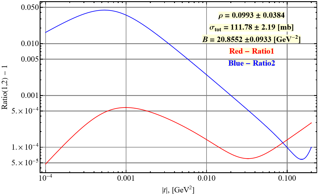The deviation from the reference values as seen at Fig. 10 demonstrates that the account for the $\mathcal{O}(\alpha^{2})$ terms in the amplitude gets more and more essential with decreasing $\mid t\mid$ . Hereof their influence on the forward observables, first of all the $\rho$-parameter.

How to explain an evident imparity of the two ratios in Fig.10 with respect to account for the $\alpha^{2}$ terms? If two amplitudes differ in their phases only they may differ significantly in the form of the amplitude. Nonetheless, they give the same result for the cross-section, both in all-order or when retaining a few terms in $\alpha$. However, if we deal with physically non-equivalent amplitudes, the results may differ significantly. In particular, non-equivalent amplitudes differently react to the inclusion of higher orders in $\alpha$. What we deal with in our case is an evident physical non-equivalence of the two amplitude moduli in question.

Appendix B. Point like electric charges.

We believe it is instructive to consider the idealized case of ”electrically point like” protons with $\mathcal{F}=1$. In this case one can obtain explicit all-order expressions.

In case of ”electrically point like” protons, i.e. if $\mathcal{F}=1$, we would have a compact explicit expression for the Coulomb kernel $S^{C}(q^{{}^{\prime}},q^{{}^{\prime\prime}})$ expressed in terms of the well known generalized functions described, e.g., in [15]:

$$S^{C}(q^{{}^{\prime}},q^{{}^{\prime\prime}})=(4\pi\alpha)^{2}\frac{(q^{{}^{\prime\prime}2}/q^{{}^{\prime}2})^{i\alpha}}{q^{{}^{\prime}2}q^{{}^{\prime\prime}2}}.$$

Physically the use of such an approximation would be justified if the average impact parameter between the colliding protons were much larger than the ”charge radius” of the proton. If (with some reservation) we take as the average transverse distance between the centres of colliding protons the value $\sqrt{2B(s)}\approx\langle b^{2}\rangle^{1/2}$, where $B(s)$ is the forward slope, then it exceeds (at $\sqrt{s}=13$ TeV) the size of the ”valence core” ($\approx 0.63$ fm) [18] only two times.

Nonetheless, we will analyse, in the end of this Section, such an option vs the TOTEM data in order that afterwards, when using a realistic form factor ($\mathcal{F}\neq 1$), to see better the influence of smearing of the electric charge of the proton.

Eqs.(2) and (3) allow to transform Eq.(1) into an all-order (in $\alpha$) expression

$$\frac{d\sigma_{C+N}}{dt}=\frac{(1+\rho^{2})\sigma^{2}_{\mbox{tot}}\mbox{exp}(-Bq^{2})}{16\pi(\hbar c)^{2}}\cdot\left|\leavevmode\nobreak\ \Gamma(1+i\alpha)\leavevmode\nobreak\ _{1}F_{1}(i\alpha,1;z)\leavevmode\nobreak\ \right|^{2}-\leavevmode\nobreak\ \leavevmode\nobreak\ \leavevmode\nobreak\ \leavevmode\nobreak\ \leavevmode\nobreak\ \leavevmode\nobreak\ \leavevmode\nobreak\ \leavevmode\nobreak\ \leavevmode\nobreak\ \leavevmode\nobreak\ \leavevmode\nobreak\ \leavevmode\nobreak\ \leavevmode\nobreak\ \leavevmode\nobreak\ \leavevmode\nobreak\ \leavevmode\nobreak\ \leavevmode\nobreak\ \leavevmode\nobreak\ \leavevmode\nobreak\ \leavevmode\nobreak\ \leavevmode\nobreak\ \leavevmode\nobreak\ \leavevmode\nobreak\ \leavevmode\nobreak\ \leavevmode\nobreak\ \leavevmode\nobreak\ \leavevmode\nobreak\ \leavevmode\nobreak\ \leavevmode\nobreak\ \leavevmode\nobreak\ \leavevmode\nobreak\ \leavevmode\nobreak\ \leavevmode\nobreak\ \leavevmode\nobreak\ \leavevmode\nobreak\ \leavevmode\nobreak\ \leavevmode\nobreak\ \leavevmode\nobreak\ \leavevmode\nobreak\ \leavevmode\nobreak\ \leavevmode\nobreak\ \leavevmode\nobreak\ \leavevmode\nobreak\ \leavevmode\nobreak\ \leavevmode\nobreak\ \leavevmode\nobreak\ \leavevmode\nobreak\ \leavevmode\nobreak\ \leavevmode\nobreak\ \leavevmode\nobreak\$$

$$-\alpha\frac{\sigma_{\mbox{tot}}}{q^{2}}\mbox{exp}\left(\frac{-Bq^{2}}{2}\right)\cdot\mbox{Re}\left\{(\rho-i)\cdot\exp\left[-i\alpha\ln\left(\frac{Bq^{2}}{2}\right)\right]\cdot\Gamma(1+i\alpha)\leavevmode\nobreak\ _{1}F_{1}(i\alpha,1;z)\right\}+\alpha^{2}\frac{4\pi(\hbar c)^{2}}{q^{4}}$$ (12)

Here ${}_{1}F_{1}(i\alpha,1;z)$ is one of the confluent hyper geometric functions (see Chapter 9.21 in [24]): At energies up to 13 TeV and $q^{2}=-t\lesssim\ 0.05\leavevmode\nobreak\ \mbox{GeV}^{2}$ the values of $z=B(s)q^{2}/2$ if of order 0.5 or less. At such $z$ the function $\Gamma(1+i\alpha)\leavevmode\nobreak\ _{1}F_{1}(i\alpha,1;z)$ is extremely close to 1 and is exhaustively approximated by the following expression

$$\Gamma(1+i\alpha)_{1}F_{1}(i\alpha,1;z)=1+i\alpha f(z)-\alpha^{2}g(z)$$

where

$$f(z)=\sum_{n=1}^{\infty}\frac{z^{n}}{nn!}-\mathcal{C}$$

and

$$g(z)=\sum_{n=1}^{\infty}\frac{z^{n}\psi(n)}{nn!}+\frac{\mathcal{C}^{2}}{2}+\frac{\pi^{2}}{12},\leavevmode\nobreak\ \leavevmode\nobreak\ \leavevmode\nobreak\ \mathcal{C}=0.5772...$$

With account of Eqs. (4) and (5) we get the following expression for the differential cross-section

$$\frac{d\sigma_{C+N}}{dt}\left[\mbox{mb/GeV}^{2}\right]=\frac{(1+\rho^{2})\sigma_{\mbox{tot}}^{2}}{16\pi(\hbar c)^{2}}e^{Bt}-\alpha\frac{\rho\cdot\sigma_{\mbox{tot}}}{\mid t\mid}e^{Bt/2}+\leavevmode\nobreak\ \leavevmode\nobreak\ \leavevmode\nobreak\ \leavevmode\nobreak\ \leavevmode\nobreak\ \leavevmode\nobreak\ \leavevmode\nobreak\ \leavevmode\nobreak\ \leavevmode\nobreak\ \leavevmode\nobreak\ \leavevmode\nobreak\ \leavevmode\nobreak\ \leavevmode\nobreak\ \leavevmode\nobreak\ \leavevmode\nobreak\ \leavevmode\nobreak\ \leavevmode\nobreak\ \leavevmode\nobreak\ \leavevmode\nobreak\ \leavevmode\nobreak\ \leavevmode\nobreak\ \leavevmode\nobreak\ \leavevmode\nobreak\ \leavevmode\nobreak\ \leavevmode\nobreak\ \leavevmode\nobreak\ \leavevmode\nobreak\ \leavevmode\nobreak\ \leavevmode\nobreak\ \leavevmode\nobreak\ \leavevmode\nobreak\ \leavevmode\nobreak\ \leavevmode\nobreak\ \leavevmode\nobreak\ \leavevmode\nobreak\ \leavevmode\nobreak\ \leavevmode\nobreak\ \leavevmode\nobreak\ \leavevmode\nobreak\ \leavevmode\nobreak\ \leavevmode\nobreak\ \leavevmode\nobreak\ \leavevmode\nobreak\ \leavevmode\nobreak\ \leavevmode\nobreak\ \leavevmode\nobreak\ \leavevmode\nobreak\ \leavevmode\nobreak\ \leavevmode\nobreak\ \leavevmode\nobreak\ \leavevmode\nobreak\ \leavevmode\nobreak\ \leavevmode\nobreak\ \leavevmode\nobreak\ \leavevmode\nobreak\ \leavevmode\nobreak\ \leavevmode\nobreak\ \leavevmode\nobreak\ \leavevmode\nobreak\ \leavevmode\nobreak\ \leavevmode\nobreak\ \leavevmode\nobreak\$$ (13)

$$\leavevmode\nobreak\ \leavevmode\nobreak\ \leavevmode\nobreak\ \leavevmode\nobreak\ \leavevmode\nobreak\ \leavevmode\nobreak\ \leavevmode\nobreak\ \leavevmode\nobreak\ \leavevmode\nobreak\ \leavevmode\nobreak\ \leavevmode\nobreak\ \leavevmode\nobreak\ \leavevmode\nobreak\ \leavevmode\nobreak\ \leavevmode\nobreak\ \leavevmode\nobreak\ \leavevmode\nobreak\ \leavevmode\nobreak\ \leavevmode\nobreak\ \leavevmode\nobreak\ \leavevmode\nobreak\ \leavevmode\nobreak\ \leavevmode\nobreak\ \leavevmode\nobreak\ \leavevmode\nobreak\ \leavevmode\nobreak\ \leavevmode\nobreak\ \leavevmode\nobreak\ \leavevmode\nobreak\ \leavevmode\nobreak\ \leavevmode\nobreak\ \leavevmode\nobreak\ +\alpha^{2}\left\{\frac{4\pi(\hbar c)^{2}}{t^{2}}-\frac{\sigma_{\mbox{tot}}}{|t|}e^{Bt/2}\left[f(z)-\mbox{ln}z\right]+\frac{(1+\rho^{2})\sigma_{\mbox{tot}}^{2}}{16\pi(\hbar c)^{2}}e^{Bt}\left[f^{2}(z)-2g(z)\right]\right\}.$$

We remind that $z=B(s)q^{2}/2\equiv Bq^{2}/2\equiv-Bt/2\equiv B|t|/2.$

Let us use Eq.(12) for description of the TOTEM data in the Coulomb-nuclear interference region. We omit repeating of several steps similar to those explained in the case of realistic form factors and show the final result. We also do not include the plots which are practically identical to those with the dipole form factor.

So, the values of the three standard parameters resulting from the description of the data under the assumption of ”electrically point-like protons” ($\mathcal{F}=1$) are as follows:

$$\sigma_{\mbox{tot}}^{\leavevmode\nobreak\ pp}=111.8\pm 2.2\mbox{ mb},$$

$$B^{\leavevmode\nobreak\ pp}=20.85\pm 0.09\mbox{ GeV}^{-2},$$

$$\rho=0.10\pm 0.04,$$

$$0.01\lesssim|t|\lesssim 0.05\mbox{ GeV}^{2}.$$

We have to emphasize that the use of the $\mathcal{O}(\alpha^{2})$ approximation appears practically equal to the use of the exect expression (11) (in more detail see Eq. (17)).

When looking at the values of parameters $\rho,\leavevmode\nobreak\ \sigma_{\mbox{tot}},\leavevmode\nobreak\ B$ one should pay attention that in spite of our ignoring the form factor effects the results almost coincide with those obtained with full account of the form factor.

In Appendix A we remarked that the CKL scheme (if corrected with inclusion of the second order term in the amplitude) in the point like limit (at $\mathcal{F}=1$) is identical to the ours, i.e. the correct one. Here, however, we take for comparison the original expression for the amplitude in the point like case [9].

The 1st order CKL amplitude for a point like electric charge is of the form (we use a special designation $\hat{T}^{CKL}_{C+N}$ for an identical remake of the corresponding expressions for the full amplitude in the original versions [9], viz Eq. (17) in the first reference in [9] and Eq. (24) in the second one:

$$\hat{T}^{CKL}_{C+N}\mid_{\mathcal{F}=1}=T_{N}(q^{2})-\frac{8\pi\alpha s}{q^{2}}+i\alpha\int_{0}^{p^{2}}\frac{dk^{2}}{k^{2}}[T_{N}(q^{2})-\bar{T}_{N}(k^{2},q^{2})].$$

So, for $T_{N}$ as in Eq. (6) we have explicitly

$$\hat{T}^{CKL}_{C+N}=T_{N}(q^{2})-\frac{8\pi\alpha s}{q^{2}}+i\alpha T_{N}(q^{2})\left[\ln\left(\frac{Bp^{2}}{2}\right)+\mathcal{C}-\sum_{n=1}^{\infty}\left(\frac{Bq^{2}}{2}\right)^{n}/n!n\right].$$ (14)

As we can see, the limit $s\rightarrow\infty$ in the upper integration limit is no longer possible and we get

$$\frac{d\hat{\sigma}_{C+N}^{CKL}}{dt}\mid_{\mathcal{F}=1}=\frac{\sigma^{2}_{\mbox{tot}}e^{-Bq^{2}}}{16\pi(\hbar c)^{2}}-\alpha\frac{\rho(s)\sigma_{\mbox{tot}}}{q^{2}}e^{Bq^{2}/2}+\alpha^{2}\left\{\frac{4\pi(\hbar c)^{2}}{q^{4}}\right.+\leavevmode\nobreak\ \leavevmode\nobreak\ \leavevmode\nobreak\ \leavevmode\nobreak\ \leavevmode\nobreak\ \leavevmode\nobreak\ \leavevmode\nobreak\ \leavevmode\nobreak\ \leavevmode\nobreak\ \leavevmode\nobreak\ \leavevmode\nobreak\ \leavevmode\nobreak\ \leavevmode\nobreak\ \leavevmode\nobreak\ \leavevmode\nobreak\ \leavevmode\nobreak\ \leavevmode\nobreak\ \leavevmode\nobreak\ \leavevmode\nobreak\ \leavevmode\nobreak\ \leavevmode\nobreak\ \leavevmode\nobreak\ \leavevmode\nobreak\ \leavevmode\nobreak\ \leavevmode\nobreak\ \leavevmode\nobreak\ \leavevmode\nobreak\ \leavevmode\nobreak\ \leavevmode\nobreak\ \leavevmode\nobreak\ \leavevmode\nobreak\ \leavevmode\nobreak\ \leavevmode\nobreak\ \leavevmode\nobreak\ \leavevmode\nobreak\ \leavevmode\nobreak\ \leavevmode\nobreak\ \leavevmode\nobreak\ \leavevmode\nobreak\ \leavevmode\nobreak\ \leavevmode\nobreak\ \leavevmode\nobreak\ \leavevmode\nobreak\ \leavevmode\nobreak\ \leavevmode\nobreak\ \leavevmode\nobreak\ \leavevmode\nobreak\ \leavevmode\nobreak\ \leavevmode\nobreak\ \leavevmode\nobreak\ \leavevmode\nobreak\ \leavevmode\nobreak\ \leavevmode\nobreak\ \leavevmode\nobreak\ \leavevmode\nobreak\ \leavevmode\nobreak\ \leavevmode\nobreak\ \leavevmode\nobreak\ \leavevmode\nobreak\ \leavevmode\nobreak\$$

$$\leavevmode\nobreak\ \leavevmode\nobreak\ \leavevmode\nobreak\ \leavevmode\nobreak\ \leavevmode\nobreak\ \leavevmode\nobreak\ \leavevmode\nobreak\ \leavevmode\nobreak\ \leavevmode\nobreak\ \leavevmode\nobreak\ \leavevmode\nobreak\ \left.+\frac{\ln\left(\frac{Bp^{2}}{2}\right)+\mathcal{C}-\sum_{n=1}^{\infty}\left(\frac{Bq^{2}}{2}\right)^{n}/n!n}{q^{2}}\sigma_{\mbox{tot}}e^{-Bq^{2}/2}+\frac{\left[\ln\left(\frac{Bp^{2}}{2}\right)-\sum_{n=1}^{\infty}\left(\frac{Bq^{2}}{2}\right)^{n}/n!n\right]^{2}}{16\pi(\hbar c)^{2}}\sigma^{2}_{\mbox{tot}}e^{-Bq^{2}}\right\},$$

where $\mathcal{C}=0.5772...$.

If we take equation for $d\hat{\sigma}_{C+N}^{CKL}/dt$ for fitting the data we get the following result for our basic parameters

$$\sigma_{\mbox{tot}}^{\leavevmode\nobreak\ pp}=111.81\pm 1.75\mbox{\leavevmode\nobreak\ mb},$$ (15)

$$B^{\leavevmode\nobreak\ pp}=20.76\pm 0.30\mbox{ GeV}^{-2},$$

$$\rho=0.2740\pm 0.0098,$$

$$\mid t\mid\lesssim 0.015\mbox{ GeV}^{2}.$$

In this case, the curve systematically passes below the central values of the experimental points (the PPP effect, see [16]), which, as before, indicates that the systematic errors are overdetermined. However, the value of the $\rho$-parameter turns out to be unexpectedly high. This probably indicates an incomplete account for terms of the second order in $\alpha$. Nonetheless, the values of $\sigma_{\mbox{tot}}$ and $B$ turn out to be quite consistent (within the error) with the previously obtained values.

Thus, we see that the point like limit according to [9] leads to the values of the basic parameters Eq. (15) different from those in the case of the dipole form factor, cf with Eq. (11). However, this mainly concerns the $\rho$ parameter while the other two seem to be little sensitive to the change in the form factor account.

As above, we also have made a fit over the most confidential interval of experimental data values, i.e. at $0.01\leq|t|\leq 0.05\leavevmode\nobreak\ \mbox{GeV}^{2}$. In this case, the curve passes ideally relative to the experimental points, the parameters $\sigma_{\mbox{tot}}$ and $B$, as elsewhere above, show enviable stability, while the $\rho$-parameter undergoes a significant change remaining, however, unusually high.

$$\sigma_{\mbox{tot}}^{\leavevmode\nobreak\ pp}=112.36\pm 2.18\mbox{\leavevmode\nobreak\ mb},$$ (16)

$$B^{\leavevmode\nobreak\ pp}=20.54\pm 0.06\mbox{ GeV}^{-2},$$

$$\rho=0.2356\pm 0.0332,$$

$$0.01\lesssim|t|\lesssim 0.05\mbox{ GeV}^{2}.$$

Howbeit, we would like to point out again that the formula Eq. (14) is the result of an incorrect manipulation with divergent integrals and therefore contains UV logarithms, which are unnatural for problems related to diffraction and Coulomb-nuclear interference, as already indicated earlier in [12].

Appendix C. Expansion in $\alpha$: where to stop?

Here we give some comments on the use of perturbative expansion in the fine structure constant $\alpha$ in the narrow sense i.e. as applied to the concrete problem considered in the text.

As to the general opinion about QED as a perturbation theory, there is a conviction that the series in $\alpha$ does not converge and should be considered as an asymptotic one due to notorious non-analyticity in coupling constant at the origin. This does not preclude to some parts of the amplitudes to have convergent expansion in $\alpha$ while non-analytic terms are of a minor significance (like, say, exp$(-c/\alpha),c>0$). This is exactly what we have in Eq.(1) where the expansion in $\alpha$ has an infinite convergence radius and we tacitly assumed the absence of non-analytic terms.

However, in practice, when one deals with a truncated series in $\alpha$ one has to estimate the error of the series truncation used, i.e. to estimate the value of discarded terms. It may well happen that for some values of the additional parameters (in our case $s$ and $t$) the approximation is justified, while for others it cannot be considered as an ”approximation” at all. In the latter case one, generally, has to account for more terms in expansion parameter.

As a simple example let us consider an oversimplified account of the point-like Coulomb interaction when the full scattering amplitude is given as follows

$$T_{C+N}(s,t)=T_{N}(s,t)+\alpha\cdot 8\pi s/t.$$

If (just for illustration) we take the parameters from the Conclusion and neglect the $\rho$ value we obtain that the second ”correction” term at the ”critical value” $|t|=6.4\cdot 10^{-4}\mbox{ GeV}^{2}$ becomes equal to the ”main” and then, at lower $|t|$ surpasses it. Let us note that the lowest $|t|$ reached by the TOTEM Collaboration (at $\sqrt{s}=13$ TeV) is $|t|=8.79\cdot 10^{-4}\mbox{ GeV}^{2}$. This is already a signal that it is necessary to take into account at least the second order in $\alpha$. At the same time, at $\mid t\mid=10^{-2}\mbox{ GeV}^{2}$ the use of the first order Coulomb term is fairly justified and constitutes near $6\%$ of the main term $T_{N}$.

Sure, in more realistic cases the critical values of $|t|$ may be different but the conclusion is the same: the weight of terms in the $\alpha$ -expansion is ”running” with $|t|$.

Figure 11: Contributions of different orders of $\alpha$ in $d\sigma_{C+N}/dt$.

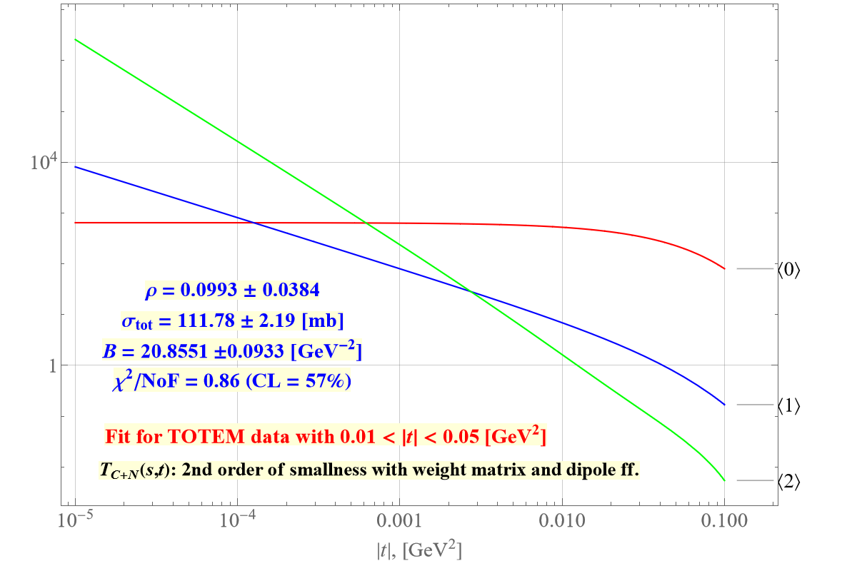Figure 11 shows that for $|t|>0.003\mbox{ GeV}^{2}$, we get the ”natural” order (we designate the n-th order as $\langle n\rangle$) i.e.

$$\langle 0\rangle>\langle 1\rangle>\langle 2\rangle.$$

At $6\cdot 10^{-4}\mbox{ GeV}^{2}<|t|<3\cdot 10^{-3}\mbox{ GeV}^{2}$ the order breaks down:

$$\langle 0\rangle>\langle 2\rangle>\langle 1\rangle$$

and, finally, at $|t|<1.3\cdot 10^{-4}\mbox{ GeV}^{2}$ the ”natural” order is broken even more, actually is reversed:

$$\langle 2\rangle>\langle 1\rangle>\langle 0\rangle.$$

This circumstance prompts us to check the error determined by the remainder term of the expansion in a series in $\alpha$ which, in this case, is the expression

$$\delta_{3}\frac{d\sigma_{C+N}}{dt}=-\alpha^{3}\frac{\rho\sigma_{\mbox{tot}}e^{-Bq^{2}/2}}{q^{2}}\left[\frac{3}{2}\ln^{2}\left(\frac{2}{Bq^{2}}\right)-\ln\left(\frac{2}{Bq^{2}}\right)\left(\mathcal{C}+\frac{1}{2}-Bq^{2}\right)-\frac{\pi^{2}}{12}\right].$$ (17)

Using parameters from Eq.(9) we are convinced that the error does not exceed a fraction of a percent of the full expression in the entire range of experimentally available values of $t$.

Thus for $10^{-4}\mbox{ GeV}^{2}\leq|t|\leq 5\cdot 10^{-2}\mbox{ GeV}^{2}$ higher orders in $\alpha$ are quite harmless and the use of Eq.(7) is fairly justified.

References

- [1] G. Antchev et al. TOTEM Collaboration. Eur.Phys.J. C79 (2019) no.9, 785, arXiv:1812.04732; CERN-EP-2017-335-v3.
- [2] E. Martynov and B. Nicolescu, EPJ Web Conf. 206 (2019) 06001.
- [3] http://hermes.ihep.su:8001/compas/kuyanov/predictor/CS/Models/index.html
- [4] V.A. Petrov, Eur.Phys.J.C 81 (2021) 670, e-Print: 2008.00990 [hep-ph].
- [5] V.A. Petrov and N.P. Tkachenko, e-Print :2201.06948 [hep-ph].
- [6] H. Bethe, Ann. Phys. 3 (1958) 190.
- [7] G.B. West and D. R. Yennie, Phys. Rev. 172, 1413(1968).
- [8] O.V. Selyugin, Phys. Rev. D 60 (1999) 074028; V. A. Petrov, E. Predazzi and A. Prokudin, Eur. Phys. J. C28 (2003) 525.
- [9] R. Cahn, Z. Phys. C15, 253 (1982); V. Kundrát and M. Lokajíček, Z. Phys. C63, 619(1994).
- [10] V. A. Petrov, Theor. Math. Phys. 204, 896–900 (2020), https://doi.org/10.1134/S0040577920070041.
- [11] A. Donnachie, P.V. Landshoff, e-Print: 2203.00290 [hep-ph].
- [12] V.A. Petrov, Eur.Phys.J. C78 (2018) no.3, 221; Erratum: Eur.Phys.J. C78 (2018) no.5, 414.
- [13] V. A. Petrov, Proc.Steklov Inst.Math. 309 (2020) 1, 219-224; e-Print:2001.06220 [hep-ph].
- [14] V. V. Ezhela, V.A. Petrov and N. P. Tkachenko, Phys.At.Nucl. 84 (2021) 3, 298-313.
- [15] I. M. Gel’fand and G. E. Shilov, Generalized Functions, Volume 1: Properties and Operations, AMS Chelsea Publishing: An Imprint of the American Mathematical Society, 1964.
- [16] R. Frühwirth, D. Neudecker and H. Leeb, EPJ Web of Conferences, 27 (2012)00008 .
- [17] V.V. Ezhela, Data Science Journal, Volume 6, Supplement, 13 October 2007, S 676-689; https://datascience.codata.org/articles/abstract/492/.
- [18] V.A. Petrov and V.A. Okorokov, Int.J.Mod.Phys.A 33 (2018) 13, 1850077, e-Print: 1802.01559 [hep-ph].
- [19] A. A. Godizov, Eur.Phys.J.C 82 (2022) 1, 56, e-Print: 2110.11895 [hep-ph]; O.V. Selyugin, e-Print: 2201.02403 [hep-ph]; M. Broilo, D.A. Fagundes, E.G.S. Luna, and M.Peláez, Phys. Rev. D 103 2021) 1, 014019, e-Print:2012.08664 [hep-ph] 014019; Atri Bhattacharya, Jean-René Cudell, Rami Oueslati, and Arno Vanthieghem, Phys. Rev. D 103(2021)5, L051502, e-Print:2012.07970 [hep-ph], L051502; A. Donnachie, P.V. Landshoff, Phys.Lett.B 798 (2019) 135008, e-Print:1904.11218 [hep-ph].
- [20] J.Procházka and V. Kundrát, Eur. Phys. J. C 80, (2020)779.
- [21] G. Antchev at al. TOTEM Collaboration, Eur. Phys. J. C 76, (2016) 661
- [22] K. Österberg, Talk at the Low-x Workshop 2021 (Elba), e-Print: 2202.03724 [hep-ex].
- [23] J. Kašpar, Acta Phys.Polon.B 52 (2021) 2, 85-97, e-Print: 2001.10227 [hep-ph];
- [24] I. S. Gradshteyn and I. M. Ryzhik, Table of Integrals, Series , and Products. Seventh Edition. A. Jeffrey(ed.), D. Zwillinger (ed.) Academic Press as an imprint of Elsevier. ISBN-13: 978-0-12-373637-6, ISBN-10:0-12-373637-4.
- [25] G. Antchev at al. TOTEM Collaboration, Eur. Phys. J. C 79, (2019) 103;