1 Introduction
For the famous linear model
|
|
|
where is the response vector, is the design matrix, is the parameter vector, and is the standardized Gaussian noise vector,
ridge regression [1], also known as
the least squares regression with Tikhonov regularization [2],
has the following form
|
|
|
(1.1) |
where
is the regularized parameter,
and the corresponding estimator is
|
|
|
In this paper, we focus only on the case , i.e., the high dimensional ridge regression. For this case, the dominant computational cost of the above estimator is from the matrix inversion which takes flops.
A straightforward way of amelioration is to solve the problem (1.1)
in the dual space. Specifically, we first solve the dual problem of (1.1),
|
|
|
(1.2) |
and the solution is
|
|
|
|
(1.3) |
Then, setting
|
|
|
|
(1.4) |
gives the estimator of (1.1) in an alternative form
|
|
|
(1.5) |
More details can be found in [3]. Now, the dominant computational cost is which appears in the computation of . However, it is still prohibitive when .
To reduce the computational cost, some scholars considered the randomized sketching technique [4, 5, 6, 7, 8, 9].
The main idea is to compress the design matrix to be a small one by post-multiplying it by a random matrix with , i.e., , and hence the reduced regression can be called the compressed ridge regression.
There are two most common ways to generate : random projection and random sampling. The former can be the (sub)Gaussian matrix [6, 7, 9], the sub-sampled randomized Hadamard transform (SRHT) [4, 5, 6, 7, 9], the sub-sampled randomized Fourier transform [7], and the CountSketch (also called the sparse embedding matrix) [6], and the latter can be the uniform sampling and the importance sampling [8].
Specifically, building on (1.3) and (1.4),
Lu et al.
[4] presented the following estimator
|
|
|
where is the SRHT and
|
|
|
(1.6) |
is the solution to the dual problem of the following compressed ridge regression
|
|
|
(1.7) |
and obtained a risk bound. Soon afterwards, for generated by the product of sparse embedding matrix and SRHT, Chen et al.
[5] developed an estimator as follows:
|
|
|
(1.8) |
where denotes the Moore-Penrose inverse, and provided an estimation error bound and a risk bound.
Later, Avron et al. [6] proposed the estimator , where
|
|
|
with being the CountSketch, SRHT, or Gaussian matrix.
The above problem is the sketch of the following regression problem
|
|
|
which is transformed from
(1.1).
Additionally, Wang et. al [7] and Lacotte and Pilanci [9] applied
the dual random projection proposed in [10, 11] to the high-dimensional ridge regression.
By the way, there are some works on compressed least squares regression [12, 13, 14, 15, 16, 17, 18, 19], which can be written in the following form
|
|
|
(1.9) |
where is typically the (sub)Gaussian matrix.
To the best of our knowledge, there is few work of applying random sampling to high-dimensional ridge regression. We only found a work of [8], which
proposed an iterative algorithm by using the random sampling with the column leverage scores or ridge leverage scores as the sampling probabilities.
This algorithm can be viewed as an extension of the method in [6]. However, there are some works on compressed least squares regression via random sampling. As far as we know, Drineas et al.
[20] first applied the random sampling with column leverage scores or approximated ones as the sampling probabilities to the least squares
regression and established the following estimator
|
|
|
which can be regarded as a special case of (1.8). Later, Slawski
[18] investigated (1.9) using uniform sampling, and discussed the predictive performance.
In this paper, we will consider the application of random sampling on high-dimensional ridge regression further. Inspired by the technique of the optimal subsampling used in e.g., [21, 22, 23, 24, 25, 26], we will mainly investigate the optimal subsampling probabilities for compressed ridge regression.
The nearly optimal subsampling probabilities and a two step iterative algorithm are also derived.
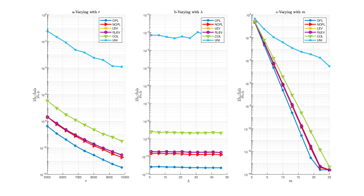
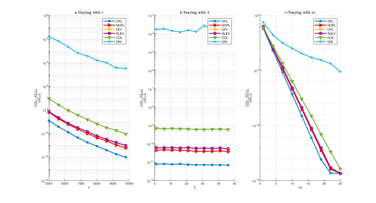
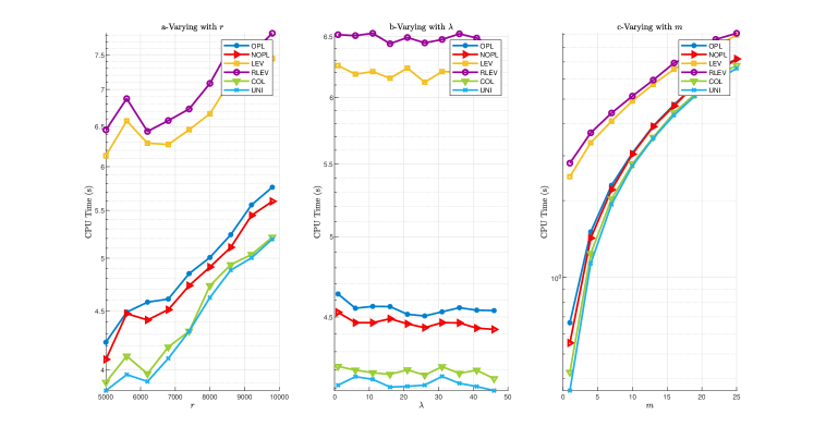
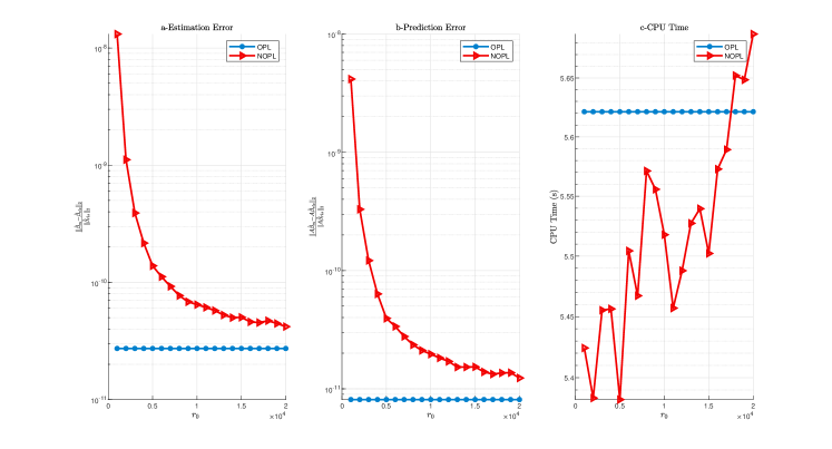
The remainder of this paper is organized as follows. The basic framework of random sampling algorithm and the optimal subsampling probabilities are presented in Section 2. In Section 3, we propose the nearly optimal subsampling probabilities and a two step iterative algorithm. The detailed theoretical analyses of the proposed methods are also presented in Sections 2 and 3, respectively. In Section 4, we provide some numerical experiments to test our methods. The proofs of all the main theorems are given in the appendix.
Before moving to the next section, we introduce some standard notations used in this paper.
For the matrix , , , and denote its -th column, -th row, spectral norm and Frobenius norm, respectively.
Also, its thin SVD is given as ,
where , , and
with the diagonal elements, i.e., the singular values of , satisfying .
For , its row norms with are the column leverage scores [8], and for , where is a diagonal matrix with the diagonal entries being (), its row norms are called the ridge leverage scores [8].
In addition, denotes that a sequence of random variables are bounded in probability and represents that the sequence convergences to zero in probability. More details can refer to [27, Chap. 2]. In our case, we also use to denote that a sequence of random variables are bounded in conditional probability given the full data matrix . Especially,
for any matrix , () means that all the elements of are bounded in probability (given ), and symbolizes that its elements are convergence to zero in probability.
Appendix A Proof of Theorem 2.1
We start by establishing two lemmas.
Lemma A.1.
Assuming that the conditions
(2.4), (2.5) and (2.6) are satisfied, we have
|
|
|
(A.1) |
where with and being as in (1.3).
Proof.
With and (1.3), it is easy to see that
|
|
|
Then, considering the basic triangle inequality and the fact that , we can have
|
|
|
|
|
|
|
|
|
|
|
|
|
|
|
|
|
|
|
|
|
|
|
|
|
|
|
|
(A.2) |
Following
|
|
|
(A.3) |
which can be derived from , and noting (2.4), (2.5),
(2.6) and (A.2), we can get
|
|
|
|
|
|
|
|
Thus, (A.1) is arrived. ∎
Lemma A.2.
Suppose that the conditions (2.5) and (2.7) hold. Then, conditional on in probability,
|
|
|
(A.4) |
|
|
|
(A.5) |
where , with constructed as in Algorithm 1, and with and being as in (1.3).
Proof.
First, note that
|
|
|
|
|
|
|
|
|
|
|
|
where the last equality is from (2.5) and (2.7).
This result implies, for any -dimensional vector with finite elements,
|
|
|
|
|
|
|
|
(A.6) |
Thus, following , it is natural to get
|
|
|
|
|
|
|
|
|
|
|
|
which together with the Markov’s inequality implies (A.4).
Combining (A) and (A.3), we can get
|
|
|
|
|
|
|
|
(A.7) |
Thus, considering
with and , and (A), we can obtain
|
|
|
|
|
|
|
|
|
|
|
|
|
|
|
|
|
|
|
|
|
|
|
|
Consequently, by the Markov’s inequality, (A.5) is obtained.
∎
Proof of Theorem 2.1. Considering that
|
|
|
|
|
|
|
|
where ,
we can rewrite as
|
|
|
|
|
|
|
|
|
|
|
|
|
|
|
|
|
|
|
|
|
|
|
|
(A.8) |
|
|
|
|
(A.9) |
where the last equality is derived by (2.7) and
Lemma A.2.
Thus, to prove (2.9),
we first prove
|
|
|
(A.10) |
Recall that with
|
|
|
Now, we construct the sequence . These random vectors are independent and identically distributed and it
is easy to get
that .
Furthermore, noting that
|
|
|
(A.11) |
which can be obtained from (2.5), together with (2.7) and (A.3),
we have
|
|
|
|
|
|
|
|
|
|
|
|
|
|
|
|
|
|
|
|
|
|
|
|
(A.12) |
|
|
|
|
(A.13) |
In addition, for any ,
we have
|
|
|
|
|
|
|
|
|
|
|
|
where the inequality is deduced by the constraint , and the last equality is from Lemma A.1. Putting the above discussions together, we find that the Lindeberg-Feller conditions are satisfied in probability. Thus, by the Lindeberg-Feller central limit theorem [27, Proposition 2.27], and noting (A.13), we can acquire
|
|
|
which combined with and gives
|
|
|
Thus, by Lemma A.2,
(A.12), and the Slutsky’s Theorem [34, Theorem 6], we can get (A.10).
Now, we prove (2.9). Following (2.7) and (A.11), it is easy to get
|
|
|
which together with (A.9) yields
|
|
|
|
|
|
|
|
(A.14) |
In addition, it is verified that
|
|
|
|
|
|
|
|
(A.15) |
Thus, combining (A.10), (A.14), and (A), by the Slutsky’s Theorem, we get the desired result (2.9).
Appendix C Proof of Theorem 2.3
We first present two auxiliary lemmas.
Lemma C.1.
[8, Theorem 23]
If , are real symmetric positive semi-definite matrices such that and , then
|
|
|
Especially,
|
|
|
Lemma C.2.
For established by ,
assuming that (2.12) holds
and letting with and , we have
|
|
|
with the probability at least .
Proof.
The proof can be accomplished along the line of the proof of [8, Theorem 3]. However, for our case,
it is necessary to note that
|
|
|
|
|
|
|
|
|
|
|
|
|
|
|
|
|
|
|
|
and
|
|
|
|
|
|
|
|
|
|
|
|
|
|
|
|
|
|
|
|
where with and . ∎
Proof of Theorem 2.3. Noting and , we can rewrite (2.13)
as
|
|
|
(C.1) |
To prove (C.1), we
define the loss functions and as
|
|
|
and
|
|
|
Thus, by Taylor expansion, we can acquire
|
|
|
(C.2) |
where and minimize the loss functions and , respectively, and .
Moreover, following
, which is from
|
|
|
and
|
|
|
(C.3) |
we can obtain
|
|
|
Thus, considering that
|
|
|
which is derived by the fact , and noting (C.2), we can gain
|
|
|
Further, by , we have
|
|
|
which together with
|
|
|
and (C.3) leads to
|
|
|
Thus, based on , it is straightforward to get
|
|
|
which is also allowed to be rewritten as
|
|
|
(C.4) |
Adding to both sides of (C.4) gives
|
|
|
|
|
|
|
|
(C.5) |
Taking the Euclidean norm on both sides of (C), we obtain
|
|
|
|
|
|
|
|
|
which combined with Lemma C.2
indicates that
|
|
|
(C.6) |
By rewriting (C.6) as
|
|
|
and considering the fact , we have
|
|
|
Thus, setting , we get (C.1). That is,
(2.13)
is arrived.
Appendix E Proof of Theorem 3.1
The proof is similar to the one of Theorem 2.1 (see Appendix A), and we begin by presenting two lemmas.
Lemma E.1.
Assume that the condition (2.6) and (3.2) hold.
Then, for and in (3.1),
we have
|
|
|
(E.1) |
where with and being as in (1.3).
Proof.
Similar to the proof of Lemma A.1, based on (2.6),
(3.1), (3.2), (A.2), and (A.3),
we have
|
|
|
|
|
|
|
|
|
|
|
|
|
|
|
|
|
|
|
|
|
|
|
|
|
|
|
|
|
|
|
|
|
|
|
|
|
|
|
|
|
|
|
|
|
|
|
|
|
|
|
|
|
|
|
|
where
the first inequality is gained by replacing in (A.2) with . Then, (E.1) is obtained.
∎
Lemma E.2.
To the assumption of Lemma E.1, add that the condition (2.7) holds. Then, for and in (3.1), conditional on and in probability,
we have
|
|
|
(E.2) |
|
|
|
(E.3) |
where , with constructed by , and with and being as in (1.3).
Proof.
The proof can be completed similar to the proof of Lemma A.2. We only need to replace with , and note that
|
|
|
|
|
|
|
|
|
|
|
|
|
|
|
|
(E.4) |
|
|
|
|
|
|
|
|
|
|
|
|
|
|
|
|
where denotes the expectation on .
Corollary E.1.
For formed by , constructed by Algorithm 2 satisfies
|
|
|
(E.5) |
Proof.
Similar to (A.8), considering (2.7) and Remark E.1, we can get
|
|
|
which suggests that (E.5) holds.
∎
Proof of Theorem 3.1. Similar to the proof of Theorem 2.1, noting (2.6), (2.7), (E.4), and Lemmas E.1 and E.2, and replacing and in the proof of Theorem 2.1 with and , respectively, we first get
|
|
|
(E.6) |
|
|
|
where
|
|
|
|
|
|
To get (3.3),
in the following, we need to further prove
|
|
|
(E.7) |
where satisfies
|
|
|
(E.8) |
Considering (2.6), (2.7), (2.10) and (3.2),
we first obtain
|
|
|
|
|
|
|
|
|
|
|
|
|
|
|
|
which indicates
|
|
|
(E.9) |
From (2.7) and (E.9), it is evident to get
|
|
|
(E.10) |
which combined with (E.6) suggests that (E.7) holds, that is,
|
|
|
|
|
|
|
|
Now, we need to demonstrate that (E.8) also holds. Evidently, it suffices to show that
|
|
|
(E.11) |
because
|
|
|
|
|
|
|
|
|
|
|
|
|
|
|
Noting
|
|
|
|
|
|
and the basic triangle inequality,
we gain
|
|
|
|
|
|
|
|
Following (2.6), (3.2), (A.3), and (E.5), it is evident to gain
|
|
|
|
|
|
|
|
|
|
|
|
|
|
|
|
|
|
|
|
Similarly, we have and . Therefore, we get
|
|
|
which combined with (2.7) and (E.10)
yields (E.11).
Putting the above discussions and the Slutsky’s Theorem together,
the result
(3.3)
follows.
