Safe Reinforcement Learning Using Black-Box Reachability Analysis
Abstract
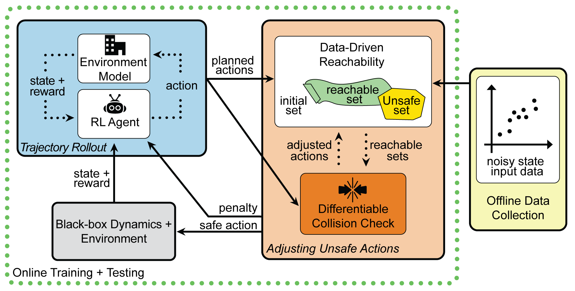
Reinforcement learning (RL) is capable of sophisticated motion planning and control for robots in uncertain environments. However, state-of-the-art deep RL approaches typically lack safety guarantees, especially when the robot and environment models are unknown. To justify widespread deployment, robots must respect safety constraints without sacrificing performance. Thus, we propose a Black-box Reachability-based Safety Layer (BRSL) with three main components: (1) data-driven reachability analysis for a black-box robot model, (2) a trajectory rollout planner that predicts future actions and observations using an ensemble of neural networks trained online, and (3) a differentiable polytope collision check between the reachable set and obstacles that enables correcting unsafe actions. In simulation, BRSL outperforms other state-of-the-art safe RL methods on a Turtlebot 3, a quadrotor, a trajectory-tracking point mass, and a hexarotor in wind with an unsafe set adjacent to the area of highest reward.
Index Terms:
Reinforcement Learning, Robot Safety, Task and Motion PlanningI Introduction
In reinforcement learning (RL), an agent perceives and reacts to consecutive states of its environment to maximize long-term cumulative expected reward [1]. One key challenge to the widespread deployment of RL in safety-critical systems is ensuring that an RL agent’s policies are safe, especially when the system environment or dynamics are a black box and subject to noise [2, 3]. In this work, we consider RL for guaranteed-safe navigation of mobile robots, such as autonomous cars or delivery drones, where safety means collision avoidance. We leverage RL to plan complex action sequences in concert with data-driven reachability analysis to guarantee safety for a black-box system.
I-A Related Work
Safe RL aims to learn policies that maximize expected reward on a task while respecting safety constraints during both learning and deployment [3]. Existing methods can be roughly classified as objective-based or exploration-based, depending on how safety is formulated. We first discuss these categories, then the specific case of mobile robot navigation, which we use to evaluate our proposed method.
Objective-based methods encourage safety by penalizing constraint violations in the objective. This can be done by relating cumulative reward to the system’s risk, such as the probability of visiting error states [4]. In practice, this results in an RL agent attempting to minimize an empirical risk measure (that is, an approximation of the probability of entering a dangerous or undesired state). Similarly, one can penalize the probability of losing reward (by visiting an unsafe state) for a given action [2], in which case the agent minimizes temporal differences in the reward and thus also minimizes risk. Another approach is to restrict policies to be ergodic with high probability, meaning any state can eventually be reached from any other state [5]. This is a more general problem, which comes at a cost: feasible safe policies do not always exist, and the algorithms are far more complex. While these methods can make an agent prefer safe actions, they cannot guarantee safety during training or deployment. Another group of objective-based algorithms aims to modify the Markov Decision Process (MDP) that the RL agent tries to optimize. Some model safe optimization problems as maximizing an unknown expected reward function [6]. However, they exploit regularity assumptions on the function wherein similar decisions are associated with similar rewards. They also assume the bandit setting, where decisions do not cause state transitions. Others utilize constrained MDPs [7] to enforce safety in various RL settings, either online or offline. Online methods learn by coupling the iteration of numerical optimization algorithms (such as primal-dual gradient updates) with data collection [8, 9, 10, 11]. These algorithms have also been studied in exploration-based settings [12, 13]. However, they provide no guarantees on safety during training. On the other hand, offline schemes separate optimization and data collection [14, 15]. They conservatively enforce safety constraints on every policy iteration but are more challenging to scale up.
Exploration-based methods modify the agent’s exploration process instead of its optimization criterion. Exploration is the process of learning about unexplored states by trying random actions or actions that are not expected to yield maximum reward (for example, an -greedy strategy). However, visiting unexplored states naïvely can harm a robot or its environment. To avoid this, one can aim to guarantee safety during both exploration and exploitation, in both training and testing, by modifying the exploration strategy to incorporate risk metrics [16]. One can also use prior knowledge as an inductive bias for the exploration process [3, 17]; for example, one can provide a finite set of demonstrations as guidance on the task [18]. Other approaches use control theory to guide or constrain the RL agent’s actions. Most of these approaches use system models with Lyapunov or control barrier functions (CBFs) to guarantee safety (or stability) of the system [19, 20, 21]. One can also combine data-driven approaches with model-free barrier or intervention functions [22, 23, 24], or use robust CBFs to model uncertain parts of a system [25, 26]. Although these approaches can provide strong guarantees, most assume the system is control-affine, and need prior knowledge on some or all of the system model [27, 28, 29], which may not always be feasible. Finally, our method is most similar to [30], which learns a safety signal from data offline, then uses it to adjust an RL agent’s controls at runtime. This method uses a first-order safety approximation for fast adjustment, but (as we show) can be conservative.
Safe navigation is a fundamental challenge in robotics, because robots typically have uncertain, nonlinear dynamics. Classical techniques such as A∗ or RRT [31, Ch. 5] have been proposed to solve the navigation problem without learning. With these methods, safety has been enforced at different levels of the planning hierarchy, such as trajectory planning [32], or low-level control [33]. More recently, however, learning-based methods have been proposed [27, 28, 29]. Some safe RL navigation approaches depend on learning a value function of the expected time that an agent takes to reach the desired goal [34, 35]. Other approaches depend on learning the actions of the robot in an end-to-end manner [36, 37, 38], meaning that the agent attempts to convert raw sensor inputs (e.g., camera or LIDAR) into actuator commands. The key advantage of RL over traditional planners is in accelerating computation time and solution quality.
I-B Proposed Method and Contributions
We propose a Black-box Reachability-based Safety Layer (BRSL), illustrated in Fig. 1, to enable strict safety guarantees for RL in an entirely data-driven way, addressing the above challenges of lacking robot and environment models a priori and of enforcing safety for uncertain systems. We note that the main advantage of BRSL is the use of data-driven methods to provide safety guarantees for black-box system dynamics. BRSL enforces safety by computing a system’s forward reachable set, which is the union of all trajectories that the system can realize within a finite or infinite time when starting from a bounded set of initial states, subject to a set of possible input signals [39]. Then, if the reachable set does not intersect with unsafe sets, the system is verified as safe, following similar arguments as in [32, 33, 40].
Limitations. Our method requires an approximation for the upper bound of a system’s Lipschitz constant, similar to [29, 41, 42]. This results in a curse of dimensionality with respect to number of samples required to approximate the constant; note other sampling-based approaches scale similarly [29, 28]. Furthermore, we focus on a discrete-time setting, assume our robot can brake to a stop, and assume accurate perception of the robot’s surroundings. We leave continuous-time (which can be addressed with similar reachability methods to ours [28, 40]) and perception uncertainty to future work.
Contributions. We show the following with BRSL:
-
1.
We propose a safety layer by integrating data-driven reachability analysis with a differentiable polytope collision check and a trajectory rollout planner.
-
2.
We demonstrate BRSL on robot navigation, where it outperforms a baseline RL agent, Reachability-based Trajectory Safeguard (RTS) [28], Safe Advantage-based Intervention for Learning policies with Reinforcement (SAILR) [24], and Safe Exploration in Continuous Action Spaces (SECAS) [30]. Our code is online.
II Preliminaries and Problem Formulation
This section presents the notation, set representations, system dynamics, and reachable set definitions used in this work. We then pose our safe RL problem.
II-A Notation and Set Representations
The -dimensional real numbers are , the natural numbers are , and the integers from to are . We denote the element at row and column of matrix by , column of by , and the element of vector by . An matrix of ones is . For and , we use the shorthand . The operator places its arguments block-diagonally in a matrix of zeros. For a pair of sets and , the Minkowski sum is , and the Cartesian product is .
We represent sets using constrained zonotopes, zonotopes, and intervals, because they enable efficient Minkowski sum computation (a key part of reachability analysis) [40] and collision checking via linear programming (critical to safe motion planning) [43]. A constrained zonotope [43] is a convex set parameterized by a center , generator matrix , constraint matrix , and constraint vector as
| (1) |
By [43, Thm. 1], every convex, compact polytope is a constrained zonotope and vice-versa. For polytopes represented as an intersection of halfplanes, we convert them to constrained zonotopes by finding a bounding box, then applying the halfspace intersection property in [44].
A zonotope is a special case of a constrained zonotope without equality constraints (but with ), which we denote . For and a linear map , we have ; we denote . The Minkowski sum of two zonotopes and is given by [40]. For an -dimensional interval with lower (resp. upper) bounds (resp. ), we abuse notation to represent it as a zonotope , with center and generator matrix .
II-B Robot and Environment
We assume the robot can be described as a discrete-time, nonlinear control system with state at time . We assume the state space is compact. The input is drawn from a zonotope at each time , where is a zonotope of all possible actions. We denote process noise by , where is specified later in Assumption 2. Finally, we denote the black box (i.e., unknown) dynamics , for which
| (2) |
We further assume that is twice differentiable and Lipschitz continuous, meaning there exists a Lipschitz constant such that, if with , then . We denote the initial state of the system as , drawn from a compact set . Note that this formulation leads to an MDP.
To enable safety guarantees, we leverage the notion of failsafe maneuvers from mobile robotics [32, 45].
Assumption 1.
We assume the dynamics are invariant to translation in position, and the robot can brake to a stop in time steps and stay stopped indefinitely. That is, there exists such that, if the robot is stopped at state , and if , then .
Note, many real robots have a braking safety controller available, similar to the notion of an invariant set [29, 28]. Also, failsafe maneuvers exist even when a robot cannot remain stationary, such loiter circles for aircraft [46, 47].
We require that process noise obeys the following assumption for numerical tractability and robustness guarantees.
Assumption 2.
Each is drawn uniformly from a noise zonotope with generators.
This formulation does not handle discontinuous changes in noise. However, there exist zonotope-based techniques to identify a change in [48], after which one can compute the system’s reachable set as in the present work. We leave measurement noise and perception uncertainty to future work. We also note, in the case of Gaussian or unbounded noise, one can overapproximate a confidence level set of a probability distribution using a zonotope [40, 48].
We denote unsafe regions of state space, or obstacles, as . We assume obstacles are static but different in each episode, as the focus of this work is not on predicting other agents’ motion. Furthermore, reachability-based frameworks exist to handle other agents’ motion [33, 49], so the present work can extend to dynamic environments.
We further assume the robot can instantaneously sense all obstacles (that is, ) and represent them as a union of constrained zonotopes. In the case of sensing limits, one can determine a minimum distance within which obstacles must be detected to ensure safety, given a robot’s maximum speed and braking distance [32, Section 5].
II-C Reachable Sets
We ensure safety by computing our robot’s forward reachable set (FRS) for a given motion plan, then adjusting the plan so that the FRS lies outside of obstacles. We define the FRS, henceforth called the reachable set, as follows:
Definition 1.
The reachable set at time step , subject to a sequence of inputs , noise , and initial set , is the set
| (3) | ||||
Recall that we treat the dynamics as a black box (e.g., a simulator), which could be nonlinear and difficult to model, but we still seek to conservatively approximate (that is, overapproximate) the reachable set .
II-D Safe RL Problem Formulation
We denote the state of the RL agent at time by , which contains the state of the robot plus information such as sensor measurements and previous actions. At each time , the RL agent chooses . Recall that denotes obstacles. For a given task, we construct a reward function (examples of are given in Section IV). At time , let denote a plan, or sequence of actions, of duration .
Then, our safe RL problem is as follows. We seek to learn a policy , represented by a neural network with parameters , that maximizes expected cumulative reward. Note that the policy can be deterministic or stochastic. Since rolling out the policy naïvely may lead to collisions, we also seek to create a safety layer between the policy and the robot (that is, to ensure for all ).
III Black-box Reachability-based Safety Layer
We unite three components into our BRSL system for collision-free motion planning without a dynamic model of the robot or its surroundings a priori. The first component is an environment model, learned online. To find high reward actions (i.e., motion plans) for this model, the second component is an RL agent. Since the agent may create unsafe plans, our third component is a safety layer that combines data-driven reachability analysis with differentiable collision checking to enable safe trajectory optimization. Theorem 1 summarizes safety via BRSL.
BRSL is summarized in Algorithm 1. It uses a receding-horizon strategy to create a new safe plan in each th receding-horizon motion planning iteration. Consider a single planning iteration (that is, time step ) (Lines 1–1). Suppose the RL agent has previously created a safe plan (such as staying stopped indefinitely). At the beginning of the iteration, BRSL creates a new plan by rolling out the RL agent along with an environment model. Next, BRSL chooses a safe action by adjusting the rolled-out action sequence (Lines 1–1) such that the corresponding reachable set (computed with Algorithm 2) is collision-free and ends with a failsafe maneuver. If the adjustment procedure (as in Algorithm 3) fails to find a safe plan, then the robot executes the failsafe maneuver. Finally, BRSL sends the first action in the current safe plan to the robot, gets a reward, and trains the RL agent and environment model (Lines 1–1). To enable training our environment model online, we collect data in a replay buffer at each time (Line 1). We note that BRSL can be used during both training and deployment. That is, the safety layer can operate even for an untrained policy. Thus, for training, we initialize with random weights.
To proceed, we detail our methods for data-driven reachability and adjusting unsafe actions.
III-A Data-Driven Reachability Analysis
BRSL performs data-driven reachability analysis of a plan using Algorithm 2, based on [42]. Algorithm 2 overapproximates the reachable set as in (3) by computing a zonotope for each time step of the current plan.
Our reachability analysis uses noisy trajectory data of the black-box system model collected offline; we use data collected online only for training the policy and environment model. We consider input-state trajectories of lengths , , with total duration . We denote the data as , , . To ease notation for the various matrix operations needed in Algorithm 2, we collect the data in matrices:
| (4a) | ||||
| (4b) | ||||
| (4c) | ||||
Note, the time steps are different in and to simplify considering state transitions corresponding to the actions in . Selecting enough data to sufficiently capture system behavior is a challenge that depends on the system, though specific sampling strategies exist for some systems [28].
We must approximate the Lipschitz constant of the dynamics for our reachability analysis, which we do from the data with the method in [42, Section 4, Remark 1]. We also require a data covering radius such that, for any data point , there exists another data point for which . We assume sufficiently many data points are known a priori to upper-bound and lower-bound ; and, we assume and are the same for offline data collection and online operation. Note, prior work assumes similar bounds [41, 42].
We find that the reachable set becomes conservative (i.e., large) if the same and are used for every dimension, because the true dynamics are typically scaled differently in each state dimension. To mitigate this source of conservativeness, we approximate a different and for each dimension, which we then use to compute a Lipschitz zonotope (see Line 2 of Algorithm 2). Note, this is an improvement over prior work [42].
III-B Adjusting Unsafe Actions
After the RL agent rolls out a plan , the safety layer adjusts it to ensure it is safe. This is done by checking the intersection of the plan’s reachable sets with unsafe sets. Note, our proposed adjustment procedure does not depend on , only on the unsafe sets around the robot. The plan is applied to the environment if all of its actions are safe; otherwise, we search for a safe plan. One strategy for finding a safe plan is to sample randomly in the action space [28], but this can be prohibitively expensive in the large action spaces that arise from choosing control inputs at multiple time steps. Instead, we use gradient descent to adjust our plan such that the reachable sets are not in collision, and such that the plan has a failsafe maneuver.
We adjust unsafe actions using Algorithm 3. If the algorithm does not complete within the duration of one time step (in other words, we fix the rate of receding-horizon planning), we terminate it and continue our previously-found safe plan. Our method steps through each action in a plan and performs the following. First, we compute the reachable set for all remaining time steps with Algorithm 2 (Line 3). Second, we collision check the reachable set (Line 3) as detailed below. Third, if the reachable sets are in a collision, we compute the gradient of the collision check and perform projected gradient descent (Line 3) as in fig 2. Finally, if the algorithm converges to a safe plan, we return it, or else return “unsafe.” Note, the final plan must have a failsafe maneuver (Line 3).
We collision check reachable and unsafe sets, all represented as constrained zonotopes, as follows. Consider two constrained zonotopes, and . Applying [43, Prop. 1], their intersection is , given by
| (5) |
We check if is empty by solving a linear program, as per [43, Prop. 2]:
| (6) |
with taken elementwise; is nonempty iff . Note, (6) is feasible when and have feasible constraints.
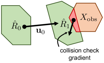
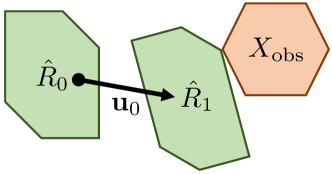
We use gradient descent to move our reachable sets out of collision. Since we use (6) for collision checking, we differentiate its solution with respect to the problem parameters using [50, 51]. Let denote the center of . Per Algorithm 2, is a function of . Let be an optimal solution to (6) when the problem parameters (i.e., the input constrained zonotopes) are and an unsafe set. Collision avoidance requires [43, Prop. 2]. We compute the gradient with respect to the input action (assuming a constant linearization point) using a chain rule recursion with given by
| (7) |
with . The gradients of are given by
| (8a) | |||
| (8b) | |||
where is computed as in Algorithm 2, Line 2, and and are the state and action dimensions. After using for gradient descent on , we project to the set of feasible controls: . The resulting controls may be unsafe, so we collision-check the final reachable sets at the end of Algorithm 3.
III-C Analyzing Safety
We conclude this section by formalizing the notion that BRSL enables safe RL.
Theorem 1.
Proof.
We prove the claim by induction on . At time , the robot can apply to stay safe for all time. Assume a safe plan exists at time . Then, if the output of Algorithm 3 is unsafe (no new plan found), the robot can continue its previous safe plan; otherwise, if a new plan is found, the plan is safe for three reasons. First, the black-box reachability in Algorithm 2 is guaranteed to contain the true reachable set of the system [42, Theorem 2], because process noise is bounded by a zonotope as in Assumption 2. Second, when adjusting an unsafe plan with Algorithm 3, the zonotope collision check is guaranteed to always detect collisions [43, Prop. 2] to assess if is empty for each time step of the plan. Third, Algorithm 3 requires that, after timesteps, the robot is stopped, so the new plan contains a failsafe manuever, and the robot can safely apply for all time . ∎
We note that the accuracy of the environment model, trained online, does not affect safety; Theorem 1 holds as long as the offline data are representative of the robot’s dynamics at runtime. We leave updating the data online for future work.
| Turtlebot | Quadrotor | |||||||||
| BRSL | RTS | SAILR | SECAS | Baseline | BRSL | RTS | SAILR | SECAS | Baseline | |
| Goal Rate [%] | 57 | 52 | 48 | 53 | 42 | 76 | 66 | 61 | 59 | 54 |
| Collision Rate [%] | 0.0 | 0.0 | 7.3 | 0.0 | 48 | 0.0 | 0.0 | 9.2 | 0.0 | 59 |
| Mean/Max Speed [m/s] | .07 / 0.18 | 0.05 / 0.15 | .07 / 0.17 | .06 / 0.15 | .08 / .18 | 3.6 / 7.9 | 3.3 / 7.8 | 3.7 / 7.9 | 3.2 / 7.8 | 3.7 / 7.9 |
| Mean Reward | 86 | 78 | 68 | 66 | 63 | 82 | 73 | 61 | 68 | 57 |
| Mean Std. Dev. | 50.41 20.5 | 100.74 60.5 | 30.53 10.8 | 22.4 14.66 | 10.21 10.05 | 60.33 20.34 | 260.85 140.67 | 45.31 20.84 | 39.7 34.08 | 20.63 30.2 |
| Compute Time [ms] | ||||||||||
| Point Environment | Hexarotor | |||||||||
| BRSL | RTS | SAILR | SECAS | Baseline | BRSL | RTS | SAILR | SECAS | Baseline | |
| Collisions [%] | 0.0 | 0.0 | 4.9 | 0.0 | 11.4 | 0.0 | 2 | 14 | 7 | 63 |
| Mean Speed [m/s] | 0.76 | 0.72 | 0.78 | 0.68 | 0.86 | 3.81 | 3.4 | 3.84 | 3.1 | 3.94 |
| Max Speed [m/s] | 2.00 | 1.89 | 2.00 | 1.74 | 2.00 | 8.4 | 8.1 | 8.2 | 7.95 | 8.7 |
| Mean Reward | 118 | 93 | 88 | 78 | 73 | 84 | 78 | 69 | 62 | 57 |
| Compute Time [ms] | 30.0 10.2 | 60.18 20.09 | 20.49 10.34 | 16.42 8.7 | 8.64 1.14 | 71.93 34.52 | 290.96 157.24 | 67.86 22.34 | 48.53 28.69 | 32.79 27.6 |
IV Evaluation
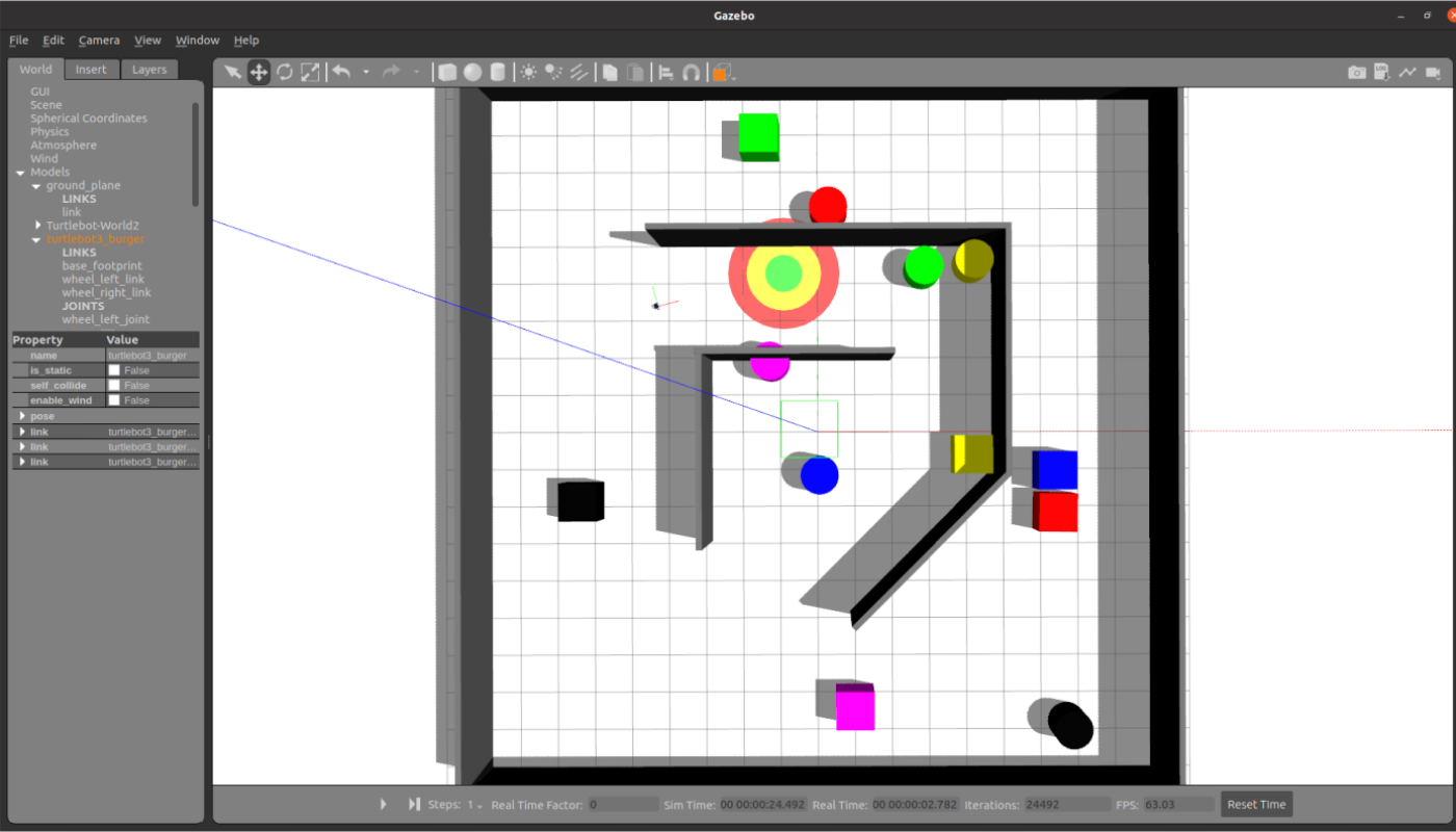
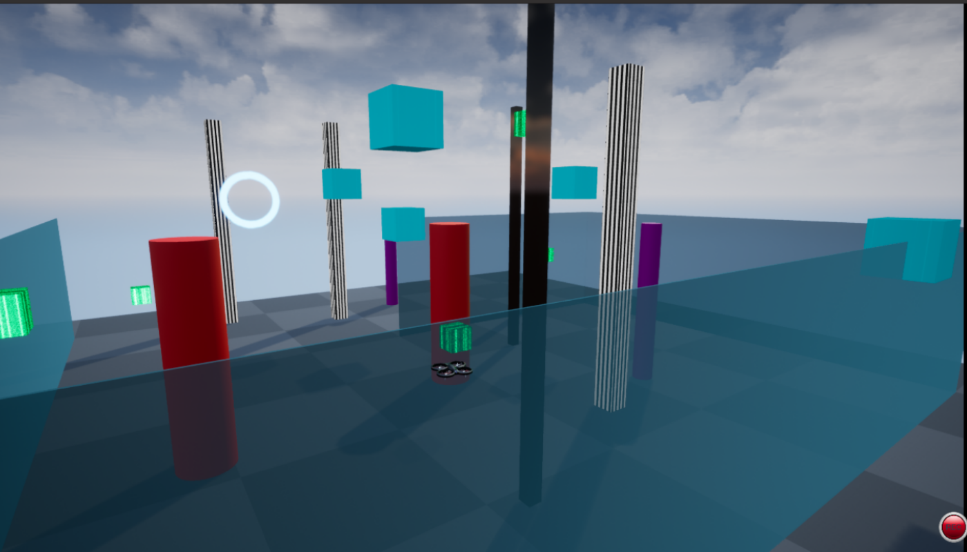
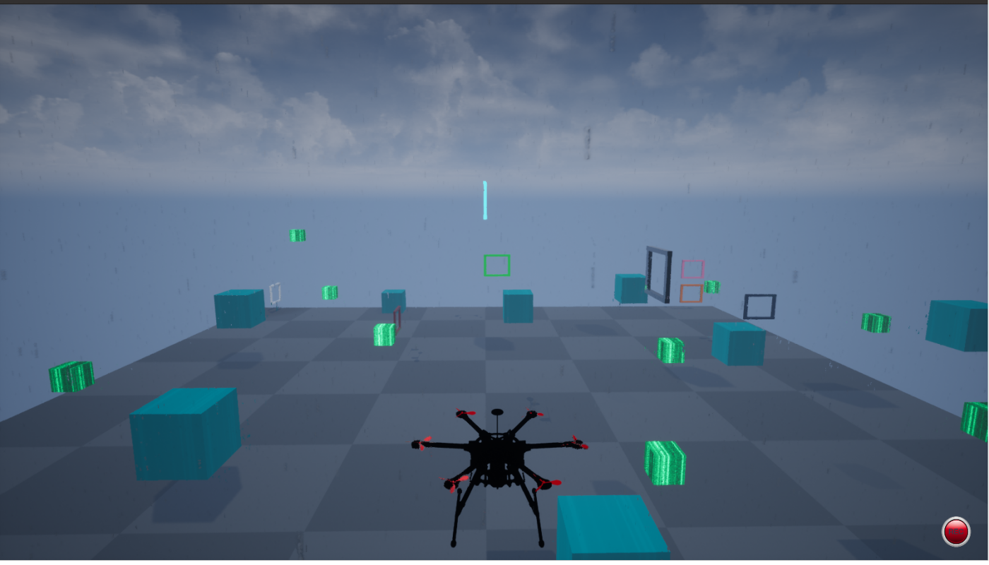
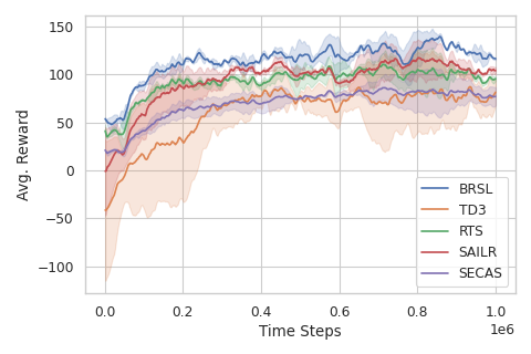
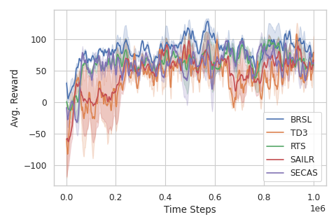
We evaluate BRSL on two types of environments: safe navigation to a goal (a Turtlebot in Gazebo and a quadrotor platform in Unreal Engine ), and path following (a point mass based on [14, 24] and a hexarotor in wind in Unreal Engine ). Figure 3 shows example environments. All code is run on a desktop computer with an Intel i5 11600 CPU and a RTX 3060 GPU. Our code is available online. We aim to assess the following: (a) How does BRSL compare against other safe RL methods (RTS [28], SAILR [24], and SECAS [30])? (b) How conservative is BRSL? (c) Can BRSL run in real time?
Setup. We use TD3 [52] as our RL agent, after determining empirically that it outperforms SAC [53] and DDPG [54]. We randomly initialize the policy. Since the agent outputs continuous actions, to aid the exploration process, we inject zero-mean Gaussian noise with a variance of that is dampened each time step. Note that this does not affect safety since our safety layer adjusts the output of the RL agent.
For each robot, to perform reachability analysis with Algorithm 2, we collect time steps of noisy state/input data (as per (4)) offline in an empty environment while applying random control inputs. We found this quantity of data sufficient to ensure safety empirically; we leave a formal analysis of the minimum amount of data for future work.
We parameterize the environment model as an ensemble of neural networks, each modeling a Gaussian distribution over future states and observations. Each network has layers, with hidden layers of size 200, and leaky ReLU activations with a negative slope of . We use a stochastic model wherein the ensemble predicts the parameters of a probability distribution, which is sampled to produce a state as in [55].
Goal-Based Environments. The Turtlebot 3 and the quadrotor seek to navigate to a random circular goal region while avoiding randomly-generated obstacles . Each robot starts in a safe location at the center of the map. Each task is episodic, ending if the robot reaches the goal, crashes, or exceeds a time limit. Both robots have uncertain, noisy dynamics as in (2). We discretize time at Hz.
The Turtlebot’s control inputs are longitudinal velocity in m/s and angular velocity in rad/s (these are the bounds of ). The robot has wheel encoders, plus a planar lidar that generates range measurements evenly spaced in a arc in front of the robot. The robot requires time steps to stop, so we set .
The quadrotor control inputs are commanded velocities up to 5 m/s in each spatial direction at each time step. We note that we also experimented with learning low-level rotor speeds versus high-level velocity commands, and found that the velocity commands created the fairest testing conditions across all agents. The robot is equipped with an IMU and a 16-channel lidar which receives range measurements around the robot in a vertical arc and a horizontal arc. The robot has , so we set .
Path Following Environments. These experiments assess BRSL’s conservativeness is by placing the highest reward adjacent to obstacles.
The goal for the point robot is to follow a circular path of radius as quickly as possible while constrained to a region smaller than the target circle. The point robot is a 2-D double integrator with position and velocity as its state: . It has a maximum velocity of 2 m/s, and its control input is acceleration up to 1 m/s2 in any direction. We use these dynamics as in [14, 24] to enable a fair test against other methods that require a robot model. We define a box-shaped safe set (the complement of the obstacle set) as , with . We use a reward that encourages traveling quickly near the unsafe set: .
The hexarotor has the same setup as the quadrotor, but with the addition of wind as an external disturbance. The goal of the hexarotor is to pass through checkpoints in a fixed order while subject to wind (constant speed and direction) and randomly-placed obstacles. Note, offline data collection was performed under wind conditions.
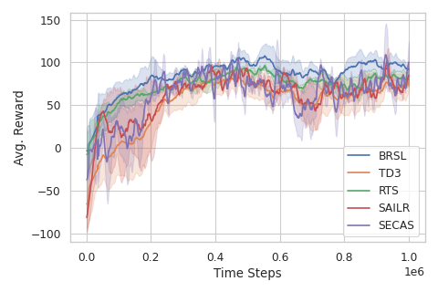
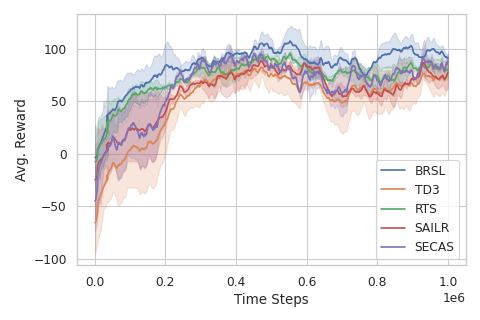
Results and Discussion. The results are summarized in Tables I and II, and in Figure 4. BRSL outperforms the other methods in terms of reward and safety, is not overly conservative, and can operate in real time, despite lacking a model of the robot a priori. While SAILR and the baseline RL agent achieved higher speeds, both experienced collisions, unlike BRSL, RTS, and SECAS. In contrast to RTS, which chooses from a low-dimensional parameterized plans, BRSL outputs a more flexible sequence of actions. Furthermore RTS’ planning time increases with state space dimension due to computing a halfspace representation of reachable set zonotopes, which grows exponentially in the number of generators [40]. BRSL avoids this computation by using (6). Instead, the quantity of data for BRSL determines the computation time of from Algorithm 2, used for reachability and adjusting unsafe actions. Therefore, one can ensure the amount of data allows real time operation; choosing the data optimally is left to future work. Finally, BRSL uses zonotopes to exactly represent safety constraints, whereas SECAS uses a more conservative first-order approximation. This results in BRSL achieving higher reward with slightly slower computation time (but still fast enough for real time operation).
V Conclusion
This paper proposes the Black-box Reachability Safety Layer, or BRSL, for safe RL without having a system model a priori. BRSL ensures safety via data-driven reachability analysis and a novel technique to push reachable sets out of collision. To enable the RL agent to make dynamics-informed decisions, BRSL also learns an environment model online, which does not affect the safety guarantee. The framework was evaluated on four robot motion planning problems, wherein BRSL respects safety constraints while achieving a high reward over time in comparison to state-of-the-art methods. For future work, we will explore continuous-time settings, reducing the conservativeness of our reachability analysis, and minimizing the amount of data needed to guarantee safety.
References
- [1] R. S. Sutton, A. G. Barto et al., Introduction to reinforcement learning. MIT press Cambridge, 1998, vol. 135.
- [2] O. Mihatsch and R. Neuneier, “Risk-sensitive reinforcement learning,” Machine learning, vol. 49, no. 2, pp. 267–290, 2002.
- [3] J. Garcıa and F. Fernández, “A comprehensive survey on safe reinforcement learning,” Journal of Machine Learning Research, vol. 16, no. 1, pp. 1437–1480, 2015.
- [4] P. Geibel and F. Wysotzki, “Risk-sensitive reinforcement learning applied to control under constraints,” Journal of Artificial Intelligence Research, vol. 24, pp. 81–108, 2005.
- [5] T. M. Moldovan and P. Abbeel, “Safe exploration in markov decision processes,” 2012.
- [6] Y. Sui, A. Gotovos, J. Burdick, and A. Krause, “Safe exploration for optimization with gaussian processes,” in Proceedings of the 32nd International Conference on Machine Learning, ser. Proceedings of Machine Learning Research, F. Bach and D. Blei, Eds., vol. 37. Lille, France: PMLR, 07–09 Jul 2015, pp. 997–1005. [Online]. Available: https://proceedings.mlr.press/v37/sui15.html
- [7] E. Altman, Constrained Markov decision processes: stochastic modeling. Routledge, 1999.
- [8] V. Borkar, “An actor-critic algorithm for constrained markov decision processes,” Systems & Control Letters, vol. 54, no. 3, pp. 207–213, 2005. [Online]. Available: https://www.sciencedirect.com/science/article/pii/S0167691104001276
- [9] Y. Chow, M. Ghavamzadeh, L. Janson, and M. Pavone, “Risk-constrained reinforcement learning with percentile risk criteria,” 2017.
- [10] C. Tessler, D. J. Mankowitz, and S. Mannor, “Reward constrained policy optimization,” 2018.
- [11] S. Bohez, A. Abdolmaleki, M. Neunert, J. Buchli, N. Heess, and R. Hadsell, “Value constrained model-free continuous control,” 2019.
- [12] D. Ding, X. Wei, Z. Yang, Z. Wang, and M. R. Jovanović, “Provably efficient safe exploration via primal-dual policy optimization,” 2020.
- [13] Y. Efroni, S. Mannor, and M. Pirotta, “Exploration-exploitation in constrained mdps,” 2020.
- [14] J. Achiam, D. Held, A. Tamar, and P. Abbeel, “Constrained policy optimization,” 2017.
- [15] H. Bharadhwaj, A. Kumar, N. Rhinehart, S. Levine, F. Shkurti, and A. Garg, “Conservative safety critics for exploration,” 2021.
- [16] C. Gehring and D. Precup, “Smart exploration in reinforcement learning using absolute temporal difference errors,” in Proceedings of the 2013 international conference on Autonomous agents and multi-agent systems, 2013, pp. 1037–1044.
- [17] R. Koppejan and S. Whiteson, “Neuroevolutionary reinforcement learning for generalized helicopter control,” in Proceedings of the 11th Annual conference on Genetic and evolutionary computation, 2009, pp. 145–152.
- [18] P. Abbeel and A. Y. Ng, “Exploration and apprenticeship learning in reinforcement learning,” in Proceedings of the 22nd international conference on Machine learning, 2005, pp. 1–8.
- [19] T. G. Molnar, R. K. Cosner, A. W. Singletary, W. Ubellacker, and A. D. Ames, “Model-free safety-critical control for robotic systems,” IEEE Robotics and Automation Letters, vol. 7, no. 2, pp. 944–951, 2021.
- [20] P. Liu, D. Tateo, H. B. Ammar, and J. Peters, “Robot reinforcement learning on the constraint manifold,” in Conference on Robot Learning. PMLR, 2022, pp. 1357–1366.
- [21] Y. Chow, O. Nachum, E. Duenez-Guzman, and M. Ghavamzadeh, “A lyapunov-based approach to safe reinforcement learning,” Advances in neural information processing systems, vol. 31, 2018.
- [22] R. Cheng, G. Orosz, R. M. Murray, and J. W. Burdick, “End-to-end safe reinforcement learning through barrier functions for safety-critical continuous control tasks,” in Proceedings of the AAAI Conference on Artificial Intelligence, vol. 33, no. 01, 2019, pp. 3387–3395.
- [23] E. Squires, R. Konda, S. Coogan, and M. Egerstedt, “Model free barrier functions via implicit evading maneuvers,” 2021. [Online]. Available: https://arxiv.org/abs/2107.12871
- [24] N. Wagener, B. Boots, and C.-A. Cheng, “Safe reinforcement learning using advantage-based intervention,” arXiv preprint arXiv:2106.09110, 2021.
- [25] M. Jankovic, “Robust control barrier functions for constrained stabilization of nonlinear systems,” Automatica, vol. 96, pp. 359–367, 10 2018.
- [26] P. Seiler, M. Jankovic, and E. Hellstrom, “Control barrier functions with unmodeled dynamics using integral quadratic constraints,” 2021. [Online]. Available: https://arxiv.org/abs/2108.10491
- [27] H. Krasowski, X. Wang, and M. Althoff, “Safe reinforcement learning for autonomous lane changing using set-based prediction,” in 2020 IEEE 23rd International Conference on Intelligent Transportation Systems (ITSC). IEEE, 2020, pp. 1–7.
- [28] Y. S. Shao, C. Chen, S. Kousik, and R. Vasudevan, “Reachability-based trajectory safeguard (rts): A safe and fast reinforcement learning safety layer for continuous control,” IEEE Robotics and Automation Letters, vol. 6, no. 2, pp. 3663–3670, 2021.
- [29] T. Lew, A. Sharma, J. Harrison, A. Bylard, and M. Pavone, “Safe active dynamics learning and control: A sequential exploration-exploitation framework,” IEEE Transactions on Robotics, 2022, in Press.
- [30] G. Dalal, K. Dvijotham, M. Vecerik, T. Hester, C. Paduraru, and Y. Tassa, “Safe exploration in continuous action spaces,” arXiv preprint arXiv:1801.08757, 2018.
- [31] S. M. LaValle, Planning algorithms. Cambridge university press, 2006.
- [32] S. Kousik, S. Vaskov, F. Bu, M. Johnson-Roberson, and R. Vasudevan, “Bridging the gap between safety and real-time performance in receding-horizon trajectory design for mobile robots,” The International Journal of Robotics Research, vol. 39, no. 12, pp. 1419–1469, 2020.
- [33] K. Leung, E. Schmerling, M. Zhang, M. Chen, J. Talbot, J. C. Gerdes, and M. Pavone, “On infusing reachability-based safety assurance within planning frameworks for human–robot vehicle interactions,” The International Journal of Robotics Research, vol. 39, no. 10-11, pp. 1326–1345, 2020.
- [34] Y. F. Chen, M. Liu, M. Everett, and J. P. How, “Decentralized non-communicating multiagent collision avoidance with deep reinforcement learning,” 2016.
- [35] Y. F. Chen, M. Everett, M. Liu, and J. P. How, “Socially aware motion planning with deep reinforcement learning,” 2018.
- [36] P. Long, T. Fan, X. Liao, W. Liu, H. Zhang, and J. Pan, “Towards optimally decentralized multi-robot collision avoidance via deep reinforcement learning,” 2018.
- [37] L. Tai, G. Paolo, and M. Liu, “Virtual-to-real deep reinforcement learning: Continuous control of mobile robots for mapless navigation,” in 2017 IEEE/RSJ International Conference on Intelligent Robots and Systems (IROS). IEEE, 2017, pp. 31–36.
- [38] L. Tai, J. Zhang, M. Liu, and W. Burgard, “Socially compliant navigation through raw depth inputs with generative adversarial imitation learning,” 2018.
- [39] Y. Ohta, H. Maeda, and S. Kodama, “Reachability, observability, and realizability of continuous-time positive systems,” SIAM journal on control and optimization, vol. 22, no. 2, pp. 171–180, 1984.
- [40] M. Althoff, “Reachability analysis and its application to the safety assessment of autonomous cars,” Ph.D. dissertation, Technische Universität München, 07 2010.
- [41] T. Koller, F. Berkenkamp, M. Turchetta, and A. Krause, “Learning-based model predictive control for safe exploration,” in 2018 IEEE conference on decision and control (CDC). IEEE, 2018, pp. 6059–6066.
- [42] A. Alanwar, A. Koch, F. Allgöwer, and K. H. Johansson, “Data-driven reachability analysis using matrix zonotopes,” in Learning for Dynamics and Control. PMLR, 2021, pp. 163–175.
- [43] J. K. Scott, D. M. Raimondo, G. R. Marseglia, and R. D. Braatz, “Constrained zonotopes: A new tool for set-based estimation and fault detection,” Automatica, vol. 69, pp. 126–136, 2016.
- [44] V. Raghuraman and J. P. Koeln, “Set operations and order reductions for constrained zonotopes,” arXiv preprint arXiv:2009.06039, 2020.
- [45] S. Magdici and M. Althoff, “Fail-safe motion planning of autonomous vehicles,” in 2016 IEEE 19th International Conference on Intelligent Transportation Systems (ITSC). IEEE, 2016, pp. 452–458.
- [46] D. Fridovich-Keil, J. F. Fisac, and C. J. Tomlin, “Safely probabilistically complete real-time planning and exploration in unknown environments,” in 2019 International Conference on Robotics and Automation (ICRA). IEEE, 2019, pp. 7470–7476.
- [47] D. Althoff, M. Althoff, and S. Scherer, “Online safety verification of trajectories for unmanned flight with offline computed robust invariant sets,” in 2015 IEEE/RSJ International Conference on Intelligent Robots and Systems (IROS). IEEE, 2015, pp. 3470–3477.
- [48] A. Shetty and G. X. Gao, “Predicting state uncertainty bounds using non-linear stochastic reachability analysis for urban gnss-based uas navigation,” IEEE Transactions on Intelligent Transportation Systems, 2020.
- [49] S. Vaskov, H. Larson, S. Kousik, M. Johnson-Roberson, and R. Vasudevan, “Not-at-fault driving in traffic: A reachability-based approach,” in 2019 IEEE Intelligent Transportation Systems Conference (ITSC). IEEE, 2019, pp. 2785–2790.
- [50] B. Amos and J. Z. Kolter, “Optnet: Differentiable optimization as a layer in neural networks,” in International Conference on Machine Learning. PMLR, 2017, pp. 136–145.
- [51] L. K. Chung, A. Dai, D. Knowles, S. Kousik, and G. X. Gao, “Constrained feedforward neural network training via reachability analysis,” 2021.
- [52] S. Dankwa and W. Zheng, “Twin-delayed ddpg: A deep reinforcement learning technique to model a continuous movement of an intelligent robot agent,” in Proceedings of the 3rd International Conference on Vision, Image and Signal Processing, 2019, pp. 1–5.
- [53] T. Haarnoja, A. Zhou, P. Abbeel, and S. Levine, “Soft actor-critic: Off-policy maximum entropy deep reinforcement learning with a stochastic actor,” 2018.
- [54] T. P. Lillicrap, J. J. Hunt, A. Pritzel, N. Heess, T. Erez, Y. Tassa, D. Silver, and D. Wierstra, “Continuous control with deep reinforcement learning,” 2019.
- [55] K. Chua, R. Calandra, R. McAllister, and S. Levine, “Deep reinforcement learning in a handful of trials using probabilistic dynamics models,” Advances in neural information processing systems, vol. 31, 2018.