CroCo: Cross-Modal Contrastive learning for localization
of Earth Observation data

Abstract

It is of interest to localize a ground-based LiDAR point cloud on remote sensing imagery. In this work, we tackle a subtask of this problem, i.e. to map a digital elevation model (DEM) rasterized from aerial LiDAR point cloud on the aerial imagery. We proposed a contrastive learning-based method that trains on DEM and high-resolution optical imagery and experiment the framework on different data sampling strategies and hyperparameters. In the best scenario, the Top-1 score of 0.71 and Top-5 score of 0.81 are obtained. The proposed method is promising for feature learning from RGB and DEM for localization and is potentially applicable to other data sources too. Source code is released at https://github.com/wtseng530/AVLocalization.

1 Introduction

The loss of geo-localization information can be critical for various applications from discarded data (processing time/money loss) to autonomous vehicles stopping due to planning failures. One possible solution to this problem is to rely on a fallback solution such as retrieving the location of the sensor by identifying the acquired data to a known, large-scale, geo-localized image map. In this study, we consider the retrieval of 3D-patch locations in large RGB scenes. The choice of these two modalities is driven by practical applications.

Target RGB data.

First, we chose the large scale data to be RGB, because it is among the most abundant available data. For example, services such as Google Maps or Bing Maps are providing high quality RGB images of the entire Earth. These are geo-referenced and can directly be linked with mapping data such as OpenStreetMaps. The reason for not directly trying to localize in abstract maps is that this type of data, while semantically complete, lacks real geometric information, helpful for geo-localization.

Lidar data.

For the source data, we chose a 3D modality, such as lidar data. This modality covers mainly two possible acquisition sources, namely aerial lidar (a) and autonomous driving lidar (b). As stated before, the loss of GPS information during the acquisition can lead to post-processing difficulties, long manual data registration, thus, human workforce and money; as well as large range of consequences, from car stopping and traffic jam inconvenience to car accident. For the particular case of autonomous driving, 3D data has advantages over ground RGB to contain the geometry, thus it is easier to change the point of view (move to bird-eye view, same as target data). Moreover, it is less subject to weather/time-of-the-day changes, e.g., day vs night.

One arising difficulty in using 3D data and RGB images, is that identifying them requires extracting the common information they contain. Common feature extractors, such as SIFT (Lowe,, 2004), HOG (Dalal and Triggs,, 2005), pretrained ImageNet models (Deng et al.,, 2009), etc., would fail, because there is no guaranty that different inputs will produce the same descriptor.

To tackle this problem, we propose jointly training two neural networks, one for RGB processing, the other for 3D processing: the two networks learn to produce similar responses to inputs of the same locations, and different for different locations. To that end, the contrastive loss introduced in SimCLR (Chen et al.,, 2020) is used to force a high feature correlation for positive data pairs, i.e. from the same locations, and low correlation for negative pairs. The resulting approach directly learns from co-registered RGB-lidar data without any additional annotation.

Additionally, to assess the validity of the proposed method, an experimental setup is designed to relocalize elevation patches in RGB data using the IEEE GRSS Data Fusion Contest 2018 dataset (Xu et al.,, 2019). The dataset contains co-located aerial images and aerial lidar scans, rasterized into elevation models and split into geographically separated training and testing data. Although elevation model is built from aerial lidar (a), it is also closely related to autonomous driving lidar (b) in the sense that elevation maps are commonly produced for automotive trajectory planning and detection.

Our contributions are thus as follow:

1. We propose a contrastive approach inspired from self-supervision models for cross-modality patch registration in large images;

2. We define, based on the DFC 2018 dataset, a 3D patch retrieval in RGB aerial images experimental setup;

3. We quantitatively and qualitatively assess that such a learning scheme can learn correlated features for cross-modal localization.

The paper is structured as following: Section 2 is dedicated to previous and related work, Section 3 describes the network architecture, Section 4 presents the dataset and Section 5 exposes the experimental results.

2 Related Work

Visual place recognition retrieves the coarse location of a target in a known scene by matching query input to a pre-built map. It is commonly approached in a two-stage manner – mapping and localizing (Bansal et al.,, 2011; Lin et al.,, 2015; Noda et al.,, 2011; Sünderhauf et al.,, 2015; Workman and Jacobs,, 2015). In the mapping stage, images or point clouds are represented by a collection of local features. These local features are then aggregated into global features, which join the corresponding camera pose or geo-referencing and forms a prior map. In the localization stage, the query data is compared with the pre-built map, and the most relevant part of the scene is retrieved as the mobile agent’s location (Chen et al.,, 2020).

Aerial and satellite imagery have become a popular source for coarse level localization and place recognition (Bansal et al.,, 2011; Chu et al.,, 2015; Kim and Walter,, 2017; Workman and Jacobs,, 2015). It resolves the challenges of viewpoint variations and appearance variations that occur in ground-based imagery (Kim and Walter,, 2017).

Lin et al., (2015) are the first to propose a deep learning method for cross-view geo-localization using Siamese CNN. Their Where-CNN model shows a significant improvement over the handcrafted features. Workman et al., (2015) match the query ground images against an aerial image database, represented by features extracted from a pre-trained model (Workman and Jacobs,, 2015). Another ground to overhead image matching explores different deep learning approaches for matching and retrieval tasks (Vo and Hays,, 2016). The authors propose a new loss function and incorporate rotation invariance and orientation regression during training. In (Cai et al.,, 2019), a hard exemplars mining strategy for cross-view matching outperforms the soft-margin triplet loss. Two CNNs are used to transform ground-level and aerial images into a common feature space. And the query ground image is localized by matching the closest geo-referenced aerial image.

An important hypothesis on which contrastive learning is built is the fact that related samples have closer embedding space. It learns feature space (or encoder) that joins related points and apart unrelated ones. Definition of related/positive and unrelated/negative is determined based on the context and objective. Positive and negative pairs can be nearby patches versus distant patches (van den Oord et al.,, 2019) or patches from the same image versus from different images. Contrastive loss is computed by contrasting latent representations of positive and negative samples. Oord et al. proposed the Noise Contrastive Estimation (NCE) which considers a random subset of negative samples for loss computation to reduce expensive computation from many negative samples (van den Oord et al.,, 2019).

SimCLR is a modified self-supervised learning algorithm for visual representation (Chen et al.,, 2020). It learns representations by maximizing the agreement between the same data example with different augmentation operations (positive pair), via a contrastive loss in the latent space.

In our work, we adapt the SimCLR architecture for a different purpose. The original SimCLR uses augmented generic images (ImageNet) to pre-train the feature encoder for downstream tasks. For us, we train on aerial imagery and elevation data without data augmentation operations. After training, the feature encoder is used directly to extract feature descriptors for localization.

3 Method

In this section, we detail the proposed approach for learning patch relocalization.

3.1 Localization Workflow

Our approach, Cross-Modal Contrastive learning for localization of Earth Observation data (CroCo), uses a two-stage visual place framework.

Mapping step.

We first create a feature map of the target, large-scale, RGB data. This map will be then used as a prior map for location queries. The features are computed using a convolutional neural network which takes as input RGB patches generated with a sliding window over the original RGB image.

Let $\phi_{\text{RGB}}$ be the transfer function of the RGB network and $\mathcal{I}_{\text{RGB}}$ be the set of patches created with the sliding window, then:

$$\mathcal{Z}_{\text{RGB}}=\left\{z_{\text{RGB}}^{i}=\phi_{\text{RGB}}\left(x_{\text{RGB}}^{i}\right)\left|\;x_{\text{RGB}}^{i}\in\mathcal{I}_{\text{RGB}}\right.\right\}$$ (1)

is the set of feature vectors that will be used for localization.

Localization step.

The second stage aims at localizing the source 3D image patch in the target RGB image. To do so, we use a second CNN, to produce a descriptor of the 3D data. This descriptor is a feature vector similar to those generated at the first stage.

Let $\phi_{\text{3D}}$ be the transfer function of this second CNN. Let $x_{\text{3D}}$ be the 3D input data, then:

$$z_{\text{3D}}=\phi_{\text{3D}}\left(x_{\text{3D}}\right)$$ (2)

is the descriptor of the input data.

Finally, the localization step is the search for the maximally correlated feature in $\mathcal{Z}_{\text{RGB}}$,

$$i^{*}=\operatorname*{argmax}_{i\;\text{s.t.}\;z_{\text{RGB}}^{i}\in\mathcal{Z}_{\text{RGB}}}\frac{{z_{\text{RGB}}^{i}}^{\top}z_{\text{3D}}}{\left\|z_{\text{RGB}}^{i}\right\|_{2}\left\|z_{\text{3D}}\right\|_{2}}$$ (3)

3.2 Cross-modal contrastive learning

For the previous framework to be efficient, $\phi_{\text{3D}}$ and $\phi_{\text{RGB}}$ must be trained jointly to produce meaningful features, i.e., features that are similar when the inputs come from the same location, and different in the other case. The goal is then to produce highly correlated features for input positive input pairs (same location) and contrasted features for negative pairs (different locations), as shown in Fig. 1.

Figure 1: Positive and negative pairs on RGB & DEM imagery.

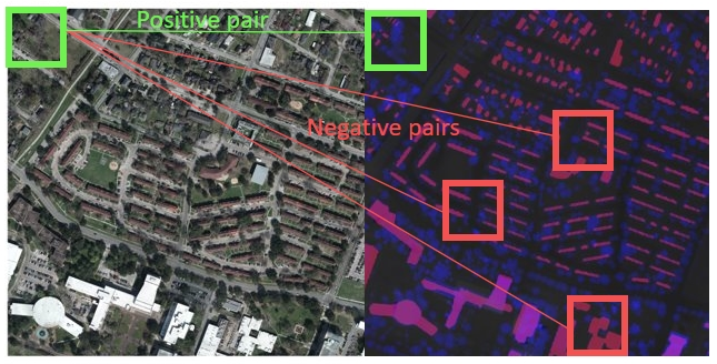
Contrastive learning is widely used in self-supervised learning. In this work we use the NT-Xent loss (the normalized temperature scaled cross-entropy loss), introduced in SimCLR (Chen et al.,, 2020):

$$l_{i,j}=-\log\dfrac{\exp\left(\text{sim}\left(z_{i},z_{j}\right)/\tau\right)}{\sum_{k=1}^{2N}{\mathbbm{1}_{[k\neq i]}\exp\left(\text{sim}\left(z_{i},z_{k}\right)/\tau\right)}}$$ (4)

where $\left(z_{i},z_{j}\right)$ is a positive pair of examples, $\tau$ denotes a temperature parameter and $\text{sim}\left(z_{i},z_{j}\right)$ is the dot product between two normalized representations $z_{i}$ and $z_{j}$:

$$\text{sim}\left(u,v\right)=\dfrac{u^{\top}v}{\left\|u\right\|\left\|v\right\|}$$ (5)

3.3 Network architecture

Figure 2: Proposed contrastive learning framework for VPR.

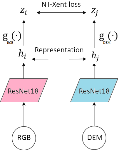
The proposed architecture is presented in Fig. 2. Each branch (RGB and elevation) is composed of a convolutional backbone and a projection head. It is similar in design to the one presented in SimCLR.

However, as our goal is to learn a cross-modal contrastive loss, each branch processes different type of data. Therefore, we do not follow a Siamese approach, and the two branches are independent (not sharing weights). Moreover, as opposed to self-supervised training, which aims at training the convolutional backbone and discards the projection head for downstream tasks, we use the full network at inference time (backbone and projection head).

Implementation details. In our experiments, we use a ResNet18 convolutional backbone and the 1-layer MLP as a projection head to map features to a 128-dimensional latent space. Please note that any convolutional backbone could be used. We chose this architecture for its relatively low memory footprint.

3.4 Training CroCo

At training time, we adapt the training procedure by Chen et al., (2020) to cross-modal data.

In each step, $N$ random positive data pairs are sampled. From these positive pairs, we build the $N(N-1)$ possible negative pairs. Each data points have one positive pair and $(N-1)$ negative pairs.

In practice, for each data input, we compute its corresponding feature vector using $\phi_{\text{RGB}}$ or $\phi_{\text{3D}}$ and the NT-Xent loss is applied for all possible data pairs (positive and negative) in the data batch.

4 Dataset

To the best of our knowledge, the proposed task, 3D data relocalization in large-scale images, has not been tackled before. Therefore, no dedicated pre-existing dataset could be found. In order to qualitatively and quantitatively assess the performances of CroCo, we repurpose the dataset GRSS_DFC_2018.

2018 Data Fusion Contest (DFC) dataset.

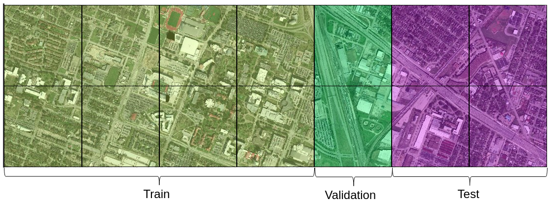
The DFC dataset (Xu et al.,, 2019) dataset by the IEEE Geoscience and Remote Sensing Society consists of multi-sensor data covering 4 km² of the University of Houston campus, which is divided into 14 image tiles, each accounting for $601\times 596$ m². The predefined tiles are split into a training set (8 tiles), validation set (2 tiles), and testing set (4 tiles) as shown in Fig. 3.

Figure 3: Train (8 tiles) / Validation (2 tiles) / Test (4 tiles) split on DFC dataset.

Modality creation.

The original dataset is designed for multi-sensor fusion and land cover classification task. We make use of the paired RGB imagery and DSM data to train a cross-modal localization model.

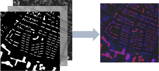
In the original dataset, four digital surface model products derived from LiDAR data are provided, namely (1) first surface model (DSM) generated from first returns, (2) bare-earth digital elevation model (DEM) from returns classified as ground, (3) bare-earth DEM with void filling for man-made structures, and (4) a hybrid ground and building DEM. We opt for the (1), (3), and (4) and concatenate them as in Fig 4.

As RGB imagery is provided in very high resolution (5cm GSD), we first need to align optical and elevation data.

Figure 4: DEM dataset created from DEM kriging, DEM triangulation, and DSM.

Objective tasks.

In order to correctly assess the performance of localization in a realistic scenario, we consider that localization is good if we retrieve the location with a given maximal error.

In this approach, we tackle this objective as a classification problem. The RGB images are split in a collection of patches using a sliding window of 2m (resp. 4m). The task is then given a 3D patch, find its corresponding patch in the image collection.

Metrics.

Following the SimCLR by Chen et al., (2020), we report Top-1 and Top-5 score. Top-1 score is the proportion of tests when the most confident retrievals, i.e. those predicted with highest probability, are the target patches (values between $[0,1]$, the higher the better). Similarly, Top-5 score is the proportion of tests when the five most confident results contain the target, thus is more relaxed than Top-1.

5 Experiments

In this section, we evaluate how a contrastive learning framework, CroCo, can generate consistent features from RGB and DEM image pairs. For the two variants of the dataset, 2m and 4m localization, we study the factors that may impact the performance of CroCo: ground sample distance (Sec 5.1), patch dimension (sec 5.2) and batch size (sec 5.3). The first two factors determine the informative detail of the input imagery, while the last is well-known for its impact in SimCLR (Chen et al.,, 2020). All these ablations are done on the validation set, as defined in the dataset section. Finally, given the set of parameters, we evaluate our model on the test set.

5.1 Ground sample distance

As RGB imagery is provided at very high ground sample distance (5cm GSD), to align optical and elevation data, we downsample the RGB images to lower resolution. Two scenarios are tested, (1) RGBs are down-sampled to 50cm GSD while DEMs are kept at 50cm GSD, and (2) RGBs and DEMs are down-sampled to 100cm GSD. The results with patch dimension of 1024 m², sample stride of 4, and batch size of 256 are shown in Tab. 1. It could be seen that the higher GSD results in higher accuracy as it provides more details of the scene.

Resolution (cm)	2m loc.		4m loc.
	Top-1	Top-5	Top-1	Top-5
50	0.43	0.57	0.40	0.55
100	0.37	0.51	0.40	0.52

Table 1: Ground sample distance study for 2m localization tasks with patch dimension of 1024 m² and batch size of 256.

5.2 Patch dimension

Patch dimension determines the spatial extension of each input tile. We consider the context of autonomous driving, in which the LIDAR sensor can receive signals up to a hundred meters. As such, 2 patch sizes are tried: 256 m², (i.e. $16\times 16$m²) and 1024 m² (i.e. $32\times 32$ m²). The results with GSD of 50cm, for the 2m localization task, and batch size of 256 are shown in Tab. 2. It could be seen that, larger patch dimension leads to better performance, as small patch size coverage leads to more patches with homogeneous appearances, hence less discriminative. This suggests that identifying an appropriate patch dimension is critical for this approach. It should be selected according to the target task.

Patch dim (m2)	Top-1	Top-5
256	0.19	0.33
1024	0.43	0.57

Table 2: Patch dimension study for 2m localization tasks with resolution of 50cm and batch size of 256.

5.3 Batch size

In contrast to supervised learning, contrastive learning benefits from the larger batch sizes. As already mentioned, each sample instance in a batch of $N$ samples generates one positive pair and $(N-1)$ negative pairs. More negative pairs available during training facilitate the convergence. We vary the batch size $N$ from 128 to 512. We adopt the LARS optimizer for all batch sizes used in SimCLR, it alleviates the unstableness yield from SDG/Momentum with linear learning rate scaling. The results are provided in Tab. 3.

In the SimCLR framework, the large batch size has been strengthened to be an important factor for contrastive learning to perform well. This is because the more samples there are in one batch, the more negative pairs we will obtain for loss computation. It takes fewer epochs and steps to get the same accuracy with the higher batch size. In the original paper, the training batch size is set from 256 to 8192. With a limited memory resource, we have to constrain our batch size to be less than 512. In general, we can observe the tendency of rising accuracy with the batch size increment. For patch size 512 m², best Top-1 and Top-5 scores are reached mostly in the highest batch size scenario.

Batch size	Top-1	Top-5
128	0.34	0.50
256	0.40	0.55
512	0.48	0.62

Table 3: Batch size study for 4m localization task with resolution of 50cm and patch dimension of 1024 m². Larger batch size results in better performance.

5.4 Evaluation on the test set

In Tab. 4, we present the results obtained on the test set. From the ablation, we chose to use the 50cm resolution data, with a patch size of 64$\times$64 (1024m²) and a batch size of 512 (the highest we can afford with our limited computational resources).

We obtain similar scores for both tasks with the same training procedure. Intuitively, the 4m localization task with higher coverage would seem easier. The main reason for not performing better in this setting resides in the way we generated the training data, following the same procedure as for the test data. Thus, using a 2m sliding window produces more training patches than for 4m. It appears that the size of the training set is also a parameter to be taken into account. We discuss it further in the discussion (Sec. 5.6).

Localization tasks	Top-1	Top-5
2m	0.64	0.80
4m	0.63	0.78

Table 4: Evaluation on the test set with ground sample distance of 50cm, patch dimension of 1024m², and batch size of 512.

5.5 Feature Representations Evaluation

In this section, we present qualitative results of CroCo.

Heatmap.

We compute similarity metrics and represent them in a heat map to understand if a positive pair of RGB and DEM image learns a comparable feature embedding. If the base encoders learn discriminative feature descriptors, then the positive pair will give the only high score in the similarity matrix. This means all the other patches are far apart in the latent space. If the similarity score for the positive pair either doesn’t give the highest score or doesn’t stand out from the rest, then the descriptor is not discriminative.

In Fig 5, we randomly plot some heat maps that visualize the similarity matrix of the target DEM patch to all RGB patches. The red box on the aerial image on the left denotes our target patch. The figure on the left is the similarity score between the query DEM descriptor against all the RGB descriptors. The value on the heat map represents the similarity score at the corresponding position. For example, the pixel at the upper left corner is the similarity score between the target patch’s DEM descriptor and the upper left most RGB patch’s descriptor. If the highest score on the heat map is indeed from the positive pair of the target, then the base encoder manages to generate a discriminative feature vector for that target. The query DEM patch is thus correctly localized.

Figure 5: Heat map generated from the similarity matrix between the target patch DEM and all RGB patches.

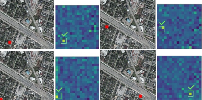
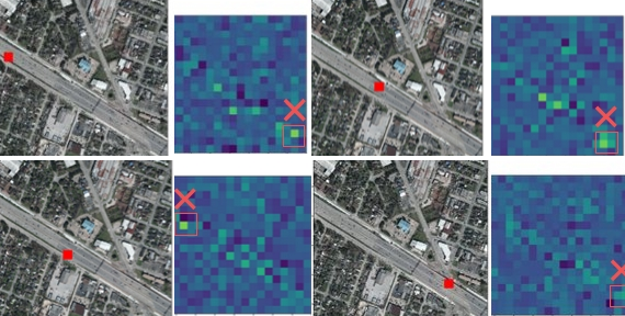
We give eight examples of localization attempts, the upper four are successful cases and the lower four are failures. In the successful cases, the target gives the highest score that strikes a clear difference from the rest patches. There are also some pixels with relatively higher scores corresponding to patches with similar structure and features as the target patch. Despite that, our method successfully retrieves the positive pair. As for our failed attempts, the mistakes mostly occur on the large traffic lane and freeway. From the heat map, we can see a strip of the bright zone that stretches along the direction of the lane. This reflects localizing in a monotonic area with less dynamic topography is difficult with our approach. As we attempt to map bird-eye view DEM to the RGB imagery, this makes it exceptionally challenging for flat areas. Considering the ground view, extra information from the street side might help with overcoming the shortage.

Localization outcome.

Figure 6: Evaluation on validation dataset.

Figure 7: Evaluation on test dataset.

Figure 8: Target RGB patches (left column) and the wrong Top-5 retrievals (following patches).

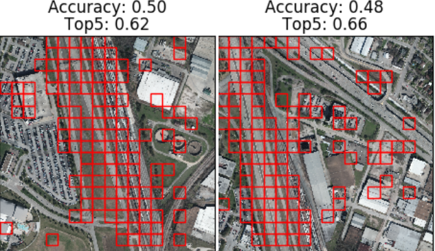
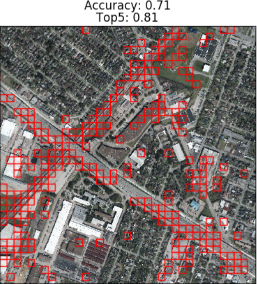
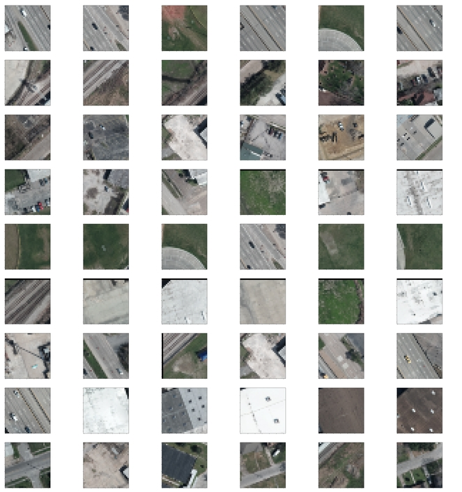
The percentage of corrected localized patches, as already explained, is denoted as the Top-1 score. Fig. 6 and Fig. 7 visualize the distribution of correct and incorrect retrievals over the map. The patches labeled with red boxes are those with the wrong Top-5 retrievals. More errors happen in flat areas such as highways, traffic lanes, rooftops, or grass areas. The phenomenon occurs in both validation and test sets. The result indicates DEM data is insufficient to give a solid localization in the area without much terrain changes. When the landscape is more diverse with complex formation, the encoder can extract invidious features and performs better localization.

In Fig. 8, we randomly select some patches that fail to retrieve the correct RGB patch in the Top-5 highest scores. The first column is the target RGB and the following five patches are the retrieved patches. We observe that the retrieved images mostly show a very similar structure and content with the target. For example, in the first two instances, all retrieved shape indicates a similar alignment with the target patch. Also for the instance 5 and 6, retrieval patches are plan areas without extra features to refer to. Our query data are DEM patches with information about the surface or terrain elevation, which lacks color information as in RGB images. Therefore, some retrieval errors that might have been easily ruled out with visual clues become difficult to avoid with the use of only a digital terrain model.

5.6 Discussion and perspectives

Training data.

As aforementioned, the size of the training dataset is of importance. We followed the same procedure to generate the training set as we did for generating the evaluation set. We use the NT-Xent loss (Chen et al.,, 2020) originating from self-supervised literature. It appears that the size of the training set along with the possible data augmentation known as critical for self-supervised learning, shall also be investigated. It is a promising perspective to deeply investigate how to enhance our training set in order to boost the performances.

Using time and context in the analysis.

We tackle the relocalization problem as a static one patch problem. In practice, acquisitions are often sequential and using the location of the previous images can help enhancing the precision of the localization and discarding the false positives. Moreover, it would allow us to create trajectories.

6 Conclusions

In this research, we proposed a contrastive learning-based method to solve the visual place recognition problem. We adapt the SimCLR framework as feature encoders trained on the contrastive loss. The augmentation operator in the original framework is replaced with our data preprocessing pipeline. Our contributions in this work are 1) Learning feature descriptors directly from contrastive learning architecture for image matching and retrieval tasks. Our method learns the feature descriptors for the RGB branch and the DEM branch simultaneously and could be used for coarse localization right after training. 2) Localize the rasterized point cloud data on the aerial image. Ground-based prior map generation and maintenance are resource-intensive. Oppositely, remote sensing-based prior maps have dense coverage, high-resolution, and are well-maintained, geo-referenced. With the use of pre-aligned aerial images and rasterized point cloud, training samples can be created simply without additional annotation work.

We conduct experiments on different sampling strategies and hyper-parameters. The proposed framework is able to learn discriminative features from RGB and DEM pairs. Despite the differences, our contrastive learning framework has demonstrated the feasibility of mapping positive data pairs into close feature embeddings for retrieval tasks. In general, the trained encoder learns to map the features correctly, and the similarity score at the target patch is notably higher than all other patches.

Our experimental result indicates that (with other factors fixed) higher image resolution gives better accuracy. However, one thing we noticed during our experiments is that with limited computation resources, the lower resolution allows a larger dataset and batch size. To sum up, resolution and computation power is compensated when applying this method for image retrieval tasks. The best performance does not necessarily come from higher image resolution with the constrain of computation power.

In correspondence to the conclusion for SimCLR, contrastive learning benefits from a larger batch size. This is because the contrastive loss is computed against all the negative pairs within the same batch, and a larger batch size creates more negative pairs. In our experiments, we notice that a larger batch size gives better Top-1 and Top-5 scores. As for the sampling stride selection, the opposite tendency is observed in 50-cm resolution and 100-cm resolution scenarios – smaller stride gives better accuracy for the former, but worse for the latter. We think it takes some further analysis to understand how the sampling stride impacts the result.

The strengths of the proposed methods are as follows: first, it is a learning-based feature, meaning no need for hand-crafting or domain-specific knowledge; second, it deals with an arbitrary input data type. The framework learns to generate identical feature vectors from the positive pairs. In our case, we define a pair of RGB and DEM imagery as our data pair. However, the input data is flexible and free of choice as long as reasonable data pair definitions are given. The weakness of the proposed method is the poor performance in localizing patches to an area with not much feature or terrain change. This is restricted by the limited information a DEM can provide. A potential solution to mitigate this weakness is to include extra data that give more context information such as the texture and color (the latter can be extracted from multispectral LiDAR sensors).

In this work, we successfully implement a contrastive learning framework to solve the localization problem using aerial RGB imagery and a rasterized point cloud. We explore different data pre-processing methodologies and also fine-tuning of the hyper-parameters. In our best scenario, we achieved 0.71 for the Top-1 score and 0.81 for the Top-5 score on the test dataset. With the heat map to visualize the similarity score between the target patch and the entire dataset, we see that the feature descriptors are discriminative and can efficiently retrieve the target patch. The proposed framework can take an arbitrary base encoder. Some future directions would be to change the backbone architecture, like a different version of ResNet. In our work, we tried only one strategy to concatenate the digital terrain models. Further analysis can be done to compare with other choices of the input data. The input data is not restricted to 2D imagery, as contrastive learning simply learns the embedding based on user-defined positive data pairs. As an extension of this research work, we are now working further on 3D point cloud data as input and corresponding 3D CNN as a base encoder.

References

- Bansal et al., (2011) Bansal, M., Sawhney, H. S., Cheng, H., Daniilidis, K., 2011. Geo-Localization of Street Views with Aerial Image Databases. ACM International Conference on Multimedia, 1125–1128.
- Cai et al., (2019) Cai, S., Guo, Y., Khan, S., Hu, J., Wen, G., 2019. Ground-to-Aerial Image Geo-Localization With a Hard Exemplar Reweighting Triplet Loss. International Conference on Computer Vision, 8390–8399.
- Chen et al., (2020) Chen, T., Kornblith, S., Norouzi, M., Hinton, G., 2020. A Simple Framework for Contrastive Learning of Visual Representations. ICML, 119, 1597–1607.
- Chu et al., (2015) Chu, H., Mei, H., Bansal, M., Walter, M. R., 2015. Accurate Vision-based Vehicle Localization using Satellite Imagery. NIPS Workshop on Transfer and Multi-Task Learning. http://arxiv.org/abs/1510.09171.
- Dalal and Triggs, (2005) Dalal, N., Triggs, B., 2005. Histograms of oriented gradients for human detection. International Conference on Computer Vision and Pattern Recognition, 886–893.
- Deng et al., (2009) Deng, J., Dong, W., Socher, R., Li, L.-J., Li, K., Fei-Fei, L., 2009. Imagenet: A large-scale hierarchical image database. 2009 IEEE Conference on Computer Vision and Pattern Recognition, 248–255.
- Kim and Walter, (2017) Kim, D.-K., Walter, M. R., 2017. Satellite image-based localization via learned embeddings. International Conference on Robotics and Automation, 2073–2080.
- Lin et al., (2015) Lin, T.-Y., Cui, Y., Belongie, S., Hays, J., 2015. Learning deep representations for ground-to-aerial geolocalization. International Conference on Computer Vision and Pattern Recognition, 5007–5015.
- Lowe, (2004) Lowe, D. D. G., 2004. Distinctive image features from scale-invariant keypoints. International Journal of Computer Vision, 60(2), 91–110.
- Noda et al., (2011) Noda, M., Takahashi, T., Deguchi, D., Ide, I., Murase, H., Kojima, Y., Naito, T., 2011. Vehicle Ego-Localization by Matching In-Vehicle Camera Images to an Aerial Image. ACCV Workshops, 163–173.
- Sünderhauf et al., (2015) Sünderhauf, N., Shirazi, S., Dayoub, F., Upcroft, B., Milford, M., 2015. On the performance of ConvNet features for place recognition. International Conference on Intelligent Robots and Systems, 4297–4304.
- van den Oord et al., (2019) van den Oord, A., Li, Y., Vinyals, O., 2019. Representation Learning with Contrastive Predictive Coding. arxiv:1807.03748.
- Vo and Hays, (2016) Vo, N. N., Hays, J., 2016. Localizing and Orienting Street Views Using Overhead Imagery. European Conference on Computer Vision, 494–509.
- Workman and Jacobs, (2015) Workman, S., Jacobs, N., 2015. On the Location Dependence of Convolutional Neural Network Features. CVPR Workshops.
- Workman et al., (2015) Workman, S., Souvenir, R., Jacobs, N., 2015. Wide-Area Image Geolocalization with Aerial Reference Imagery. International Conference on Computer Vision.
- Xu et al., (2019) Xu, Y., Du, B., Zhang, L., Cerra, D., Pato, M., Carmona, E., Prasad, S., Yokoya, N., Hansch, R., Saux, B. L., 2019. Advanced Multi-Sensor Optical Remote Sensing for Urban Land Use and Land Cover Classification: Outcome of the 2018 IEEE GRSS Data Fusion Contest. IEEE Journal of Selected Topics in Applied Earth Observations and Remote Sensing, 12(6), 1709–1724.