Entropic transfer operators

Oliver Junge, Daniel Matthes Department of Mathematics, TUM School of Computation, Information and Technology, Technical University of Munich, Germany  and  Bernhard Schmitzer Institute of Computer Science, University of Göttingen, Germany oliver.junge@tum.de, matthes@ma.tum.de, schmitzer@cs.uni-goettingen.de
Abstract.

We propose a new concept for the regularization and discretization of transfer and Koopman operators in dynamical systems. Our approach is based on the entropically regularized optimal transport between two probability measures. In particular, we use optimal transport plans in order to construct a finite-dimensional approximation of some transfer or Koopman operator which can be analysed computationally. We prove that the spectrum of the discretized operator converges to the one of the regularized original operator, give a detailed analysis of the relation between the discretized and the original peripheral spectrum for a rotation map on the n𝑛n-torus and provide code for three numerical experiments, including one based on the raw trajectory data of a small biomolecule from which its dominant conformations are recovered.

1. Introduction

1.1. Context and motivation

A time-discrete dynamical system can be described by a state space 𝒳𝒳\mathcal{X} and an evolution map F:𝒳𝒳:𝐹𝒳𝒳F:\mathcal{X}\to\mathcal{X} that specifies how points move from one time instance t𝑡t to the next: xt+1=F(xt)subscript𝑥𝑡1𝐹subscript𝑥𝑡x_{t+1}=F(x_{t}). In the case of an underlying (ordinary) differential equation, F=Fτ𝐹superscript𝐹𝜏F=F^{\tau} can be chosen to be the flow map for some fixed time step τ>0𝜏0\tau>0. A classical goal in dynamical systems theory is then to characterize how the trajectory (xt)tsubscriptsubscript𝑥𝑡𝑡(x_{t})_{t} of some initial state x0subscript𝑥0x_{0} behaves, e.g. whether it is (almost) periodic or remains in some subset of 𝒳𝒳\mathcal{X} for a long time.

However, in complicated systems (i.e. chaotic or high-dimensional) typical individual trajectories can often not be described in simple geometric terms. In chaotic systems, a trajectory exhibits sensitive dependence on its initial point, and thus the trajectory of a single initial point is of little descriptive value. In this case, it is more appropriate to describe the system in a statistical way: Consider an 𝒳𝒳\mathcal{X}-valued random variable X𝑋X with distribution μ𝜇\mu, then the distribution of F(X)𝐹𝑋F(X) is given by the push forward111with F1(A)={x𝒳:F(x)A}superscript𝐹1𝐴conditional-set𝑥𝒳𝐹𝑥𝐴F^{-1}(A)=\{x\in\mathcal{X}:F(x)\in A\} denoting the preimage of some (measurable) set A𝐴A μF1𝜇superscript𝐹1\mu\circ F^{-1} of μ𝜇\mu under the map F𝐹F. So instead of the nonlinear map F𝐹F on 𝒳𝒳\mathcal{X} we use the linear map F#:μμF1:subscript𝐹#maps-to𝜇𝜇superscript𝐹1F_{\#}:\mu\mapsto\mu\circ F^{-1} on probability measures over 𝒳𝒳\mathcal{X}, called the transfer (or Frobenius-Perron) operator in order to describe the dynamics. Relatedly, one may consider how some continuous observable φ:𝒳:𝜑𝒳\varphi:\mathcal{X}\to{\mathbb{R}} is evolved through F𝐹F, i.e. φ(xt+1)=φ(F(xt))𝜑subscript𝑥𝑡1𝜑𝐹subscript𝑥𝑡\varphi(x_{t+1})=\varphi(F(x_{t})), which yields the linear operator K:φφF:𝐾maps-to𝜑𝜑𝐹K:\varphi\mapsto\varphi\circ F, the Koopman operator. This statistical point of view has been developed in ergodic theory, cf. [31, 50, 32].

Since these two operators are linear, tools from linear functional analysis can in principle be applied in order to analyse them. However, the infinite dimensionality of the underlying function spaces and the non-compactness of the operators make a numerical approximation non-trivial. As a remedy, regularized versions of the operators can be considered which, e.g., result from (small) random perturbations of F𝐹F [24, 32]. In a suitable functional analytic setting, these regularized operators are compact, therefore have a discrete spectrum, and can be approximated numerically by a Galerkin method [14, 13].

The resulting matrix gives a simple means for a forward prediction of the dynamics by mere matrix-vector multiplication [32, 5]. It can also be used in order to construct a reduced predictive model of the system [10, 39, 27]. Finally, the nodal domains of eigenvectors at eigenvalues of large magnitude can be used in order to decompose the state space into macroscopic (almost-)cyclic or almost-invariant (i.e. metastable) components, yielding a coarse-grained model of the system [13].

This approach works well if the (Hausdorff) dimension of 𝒳𝒳\mathcal{X} is small, i.e. 3absent3\leq 3. Then, standard spaces can be used for the Galerkin approximation, e.g., piecewise constant functions, resulting in Ulam’s method [48, 34]. In the case of a high dimensional 𝒳𝒳\mathcal{X}, but a low dimensional attractor/invariant set, set oriented methods [12, 13] can be employed in order to restrict the computations to the invariant set. Recently, approximation methods have been proposed which are suited for problems with dynamics on a high dimensional invariant set. (Extended) dynamic mode decomposition [43, 53, 54] is a Petrov-Galerkin approximation of the Koopman operator with different types of ansatz functions and point evaluations as test functions [26].

1.2. Contribution and outline

The contribution of this paper is the construction of an approximation method for the transfer and via its adjoint also for the Koopman operator which also works for dynamics on high dimensional invariant sets and only uses (trajectory) data. It combines a regularization of the transfer operator through an entropically regularized optimal transport plan [49, 44, 42] with a discretization through the restriction to point masses. It bears similarities with the construction using Gaussian kernels in [28, 19]. In contrast to this and (extended) dynamic mode decomposition, though, our approach inherits important structural properties of the original operator: Our continuous and our discrete regularized operators are Markov, and they preserve the invariant measure (in the discrete setting: the uniform measure on the sample points).

θ𝜃\theta
(a)
(b)
(c)
(d)
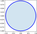
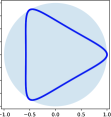
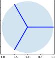
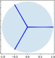
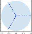
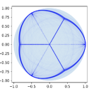
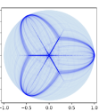
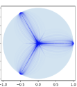
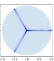
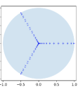
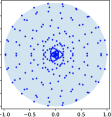
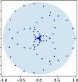
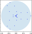
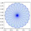
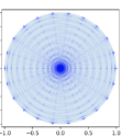
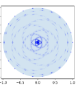
Figure 1. (A) The unit circle 𝒳=S1𝒳superscript𝑆1\mathcal{X}=S^{1} with the shift map F:φφ+θ:𝐹maps-to𝜑𝜑𝜃F:\varphi\mapsto\varphi+\theta (blue) with θ2π/3𝜃2𝜋3\theta\approx 2\pi/3 is a simple dynamical system with an approximate 3-cycle. (B) A discretization 𝒳Nsuperscript𝒳𝑁\mathcal{X}^{N} with 7 equidistant points (black) composed with a deterministic map (green) of F(𝒳N)𝐹superscript𝒳𝑁F(\mathcal{X}^{N}) (red) back to 𝒳Nsuperscript𝒳𝑁\mathcal{X}^{N} yields a single cycle of length 7 that does not reflect the approximate 3-cycle. (C) A composition with an entropic optimal transport map (green) yields a Markov chain on 𝒳Nsuperscript𝒳𝑁\mathcal{X}^{N} which inherits the almost 3-cycle (this fact is not deducible from this visualization). (D) This still holds when 𝒳Nsuperscript𝒳𝑁\mathcal{X}^{N} does not exactly lie on the attractor/invariant set and when it is distributed at random.

The approach presented here approximates the deterministic map F𝐹F on 𝒳𝒳\mathcal{X} by a stochastic model on a discrete set 𝒳Nsuperscript𝒳𝑁\mathcal{X}^{N}, which is a finite collection of points from 𝒳𝒳\mathcal{X}. By continuity of the map F𝐹F, it is reasonable to expect that macroscopic features are still observed by “probing” the dynamics only in 𝒳Nsuperscript𝒳𝑁\mathcal{X}^{N} (if this set represents 𝒳𝒳\mathcal{X} sufficiently well). However, it is not enough to simply consider the deterministic map F𝐹F restricted to 𝒳Nsuperscript𝒳𝑁\mathcal{X}^{N} since 𝒳Nsuperscript𝒳𝑁\mathcal{X}^{N} is usually not invariant under F𝐹F. A deterministic identification of points in F(𝒳N)𝐹superscript𝒳𝑁F(\mathcal{X}^{N}) and 𝒳Nsuperscript𝒳𝑁\mathcal{X}^{N} bears the danger that the resulting dynamics is dominated by combinatorial discretization artifacts (see Figure 1 for an illustration and Section 5.4 for discussion).

Instead, we propose a stochastic identification of F(𝒳N)𝐹superscript𝒳𝑁F(\mathcal{X}^{N}) and 𝒳Nsuperscript𝒳𝑁\mathcal{X}^{N} by means of an optimal transport plan with entropic regularization between distributions on F(𝒳N)𝐹superscript𝒳𝑁F(\mathcal{X}^{N}) and 𝒳Nsuperscript𝒳𝑁\mathcal{X}^{N}. Under this plan, the masses of the image points in F(𝒳N)𝐹superscript𝒳𝑁F(\mathcal{X}^{N}) are distributed such that each point in 𝒳Nsuperscript𝒳𝑁\mathcal{X}^{N} receives precisely a unit amount of mass. The optimal entropic transport plan reflects spatial proximity, i.e., the mass of a point in F(𝒳N)𝐹superscript𝒳𝑁F(\mathcal{X}^{N}) goes preferably to points in 𝒳Nsuperscript𝒳𝑁\mathcal{X}^{N} that are nearby, but it also introduces some stochastic blur on a length scale that depends on some regularization parameter ε𝜀\varepsilon.

Our approximation of the transfer operator has several attractive properties. First, as already mentioned, it is a Markovian approximation, and it preserves the invariant measure. Second, the blur introduced by the entropic regularization masks dynamic phenomena below the length scale of ε1/2superscript𝜀12\varepsilon^{1/2}, and in particular can be used to remove discretization artefacts. By varying ε𝜀\varepsilon, dynamical phenomena on specific scales can be studied. The blur further leads to compactness of the approximated transfer operator, and thus to a separation of its spectrum into a few “large” eigenvalues of modulus close to one, and the remaining “small” eigenvalues close to zero; the large eigenvalues relate to macroscopic dynamical features like cyclic or metastable behaviour, cf. [13]. Finally, the Sinkhorn algorithm provides a tool to numerically solve the underlying regularized optimal transport problems efficiently.

In [29], an approach for the detection of coherent sets in non-autonomous dynamical systems has been proposed which also uses the concept of optimal transport. There, it is assumed that two measurements of μ𝜇\mu and F#μsubscript𝐹#𝜇F_{\#}\mu are given, F𝐹F is unknown and μ𝜇\mu is not assumed to be an invariant measure of F𝐹F. The transfer operator F#subscript𝐹#F_{\#} is estimated by the optimal transport between μ𝜇\mu and F#μsubscript𝐹#𝜇F_{\#}\mu, and approximately coherent sets are subsequently estimated. Entropic smoothing provides a simple numerical algorithm, compactness of F#subscript𝐹#F_{\#} and validity of the clustering step. In contrast, we assume that an approximation μNsuperscript𝜇𝑁\mu^{N} of μ𝜇\mu and the behaviour of F𝐹F on μNsuperscript𝜇𝑁\mu^{N} are known where now μ𝜇\mu is assumed to be an invariant measure of F𝐹F. Again, entropic smoothing provides a simple numerical algorithm and compactness of the transfer operator.

We recall basic properties on transfer operators and (entropic) optimal transport in Sections 2 and 3. In Section 4, we introduce the regularized version Tεsuperscript𝑇𝜀T^{\varepsilon} of the original transfer operator T=F#𝑇subscript𝐹#T=F_{\#} and the discrete transfer operator TN,εsuperscript𝑇𝑁𝜀T^{N,\varepsilon} and establish the convergence of (an extension of) TN,εsuperscript𝑇𝑁𝜀T^{N,\varepsilon} to Tεsuperscript𝑇𝜀T^{\varepsilon} in norm. As a proof of concept, in Section 5 we analytically study the application to the shift map on the d𝑑d-torus to provide intuition for the interplay of the length scales associated to eigenfunctions of T𝑇T, discretization index N𝑁N, and entropic regularization ε𝜀\varepsilon. Several numerical examples are given in Section 6.

1.3. General hypotheses and notations

Throughout this manuscript, (𝒳,d)𝒳d(\mathcal{X},\mathrm{d}) is a compact metric space, and F:𝒳𝒳:𝐹𝒳𝒳F:\mathcal{X}\to\mathcal{X} is a continuous map. We shall occasionally assume that 𝒳𝒳\mathcal{X} is a compact subset of dsuperscript𝑑{\mathbb{R}}^{d}, but only when explicitly mentioned. Unless stated otherwise, the cost function c:𝒳×𝒳0:𝑐𝒳𝒳subscriptabsent0c:\mathcal{X}\times\mathcal{X}\to{\mathbb{R}}_{\geq 0} for optimal transportation is the canonical one, c(x,y)=d(x,y)2𝑐𝑥𝑦dsuperscript𝑥𝑦2c(x,y)=\mathrm{d}(x,y)^{2}. We denote the set of probability measures on X𝑋X by 𝒫(X)𝒫𝑋\mathcal{P}(X) and use the notation hμ𝜇h\mu in order to denote a measure which is absolutely continuous with density hh with respect to the measure μ𝜇\mu. Weak convergence of a sequence (μN)Nsubscriptsuperscript𝜇𝑁𝑁(\mu^{N})_{N} of measures to a limiting measure μ𝜇\mu is denoted by μNμsuperscriptsuperscript𝜇𝑁𝜇\mu^{N}\stackrel{{\scriptstyle\ast}}{{\rightarrow}}\mu.

2. Background on transfer operators

2.1. Push-forward and invariant measures

Choose some points x1,,xN𝒳subscript𝑥1subscript𝑥𝑁𝒳x_{1},\ldots,x_{N}\in\mathcal{X} independently according to some probability measure μ𝜇\mu on 𝒳𝒳\mathcal{X}, i.e. such that the probability 𝐏(xjB)𝐏subscript𝑥𝑗𝐵\mathbf{P}(x_{j}\in B) to find xjsubscript𝑥𝑗x_{j} in some Borel set B𝐵B is μ(B)𝜇𝐵\mu(B). Then

𝐏(F(xj)A)=𝐏(xjF1(A))=μ(F1(A)),𝐏𝐹subscript𝑥𝑗𝐴𝐏subscript𝑥𝑗superscript𝐹1𝐴𝜇superscript𝐹1𝐴\displaystyle\mathbf{P}(F(x_{j})\in A)=\mathbf{P}(x_{j}\in F^{-1}(A))=\mu(F^{-1}(A)),

i.e. the probability to find some image point F(xj)𝐹subscript𝑥𝑗F(x_{j}) in some Borel set A𝐴A is μ(F1(A))𝜇superscript𝐹1𝐴\mu(F^{-1}(A)) where we denote by F1(A)={x𝒳F(x)A}superscript𝐹1𝐴conditional-set𝑥𝒳𝐹𝑥𝐴F^{-1}(A)=\{x\in\mathcal{X}\mid F(x)\in A\} the preimage of the set A𝒳𝐴𝒳A\subset\mathcal{X}. Phrasing this differently: If some points x1,,xNsubscript𝑥1subscript𝑥𝑁x_{1},\ldots,x_{N} are distributed according to the probability measure μ𝜇\mu then their image points F(x1),,F(xN)𝐹subscript𝑥1𝐹subscript𝑥𝑁F(x_{1}),\ldots,F(x_{N}) are distributed according to the probability measure

(1) F#μ:=μ(F1()),assignsubscript𝐹#𝜇𝜇superscript𝐹1F_{\#}\mu:=\mu(F^{-1}(\cdot)),

called the push-forward measure of μ𝜇\mu (under F𝐹F). The mapping F#:μF#μ:subscript𝐹#maps-to𝜇subscript𝐹#𝜇F_{\#}:\mu\mapsto F_{\#}\mu defines a linear operator on the space of bounded signed measures, called transfer operator (or Frobenius-Perron operator). Clearly, if μ𝜇\mu is a linear combination of point measures at some points x1,,xN𝒳subscript𝑥1subscript𝑥𝑁𝒳x_{1},\ldots,x_{N}\in\mathcal{X}, i.e. μ=jajδxj𝜇subscript𝑗subscript𝑎𝑗subscript𝛿subscript𝑥𝑗\mu=\sum_{j}a_{j}\delta_{x_{j}}, ajsubscript𝑎𝑗a_{j}\in{\mathbb{R}}, then

(2) F#μ=jajδxj(F1())=jajδF(xj).subscript𝐹#𝜇subscript𝑗subscript𝑎𝑗subscript𝛿subscript𝑥𝑗superscript𝐹1subscript𝑗subscript𝑎𝑗subscript𝛿𝐹subscript𝑥𝑗F_{\#}\mu=\sum_{j}a_{j}\delta_{x_{j}}(F^{-1}(\cdot))=\sum_{j}a_{j}\delta_{F(x_{j})}.

Additionally, from (1) we directly get that F#μ0subscript𝐹#𝜇0F_{\#}\mu\geq 0 and dF#μ=dμdifferential-dsubscript𝐹#𝜇differential-d𝜇\int\;\mathrm{d}F_{\#}\mu=\int\;\mathrm{d}\mu for any non-negative measure μ𝜇\mu, i.e. F#subscript𝐹#F_{\#} is a Markov operator.

A probability measure which is a fixed point of F#subscript𝐹#F_{\#} is called an invariant measure. Invariant measures provide information about, e.g., recurrent behaviour of points:

Theorem 1 (Poincaré).

Let μ𝜇\mu be an invariant measure for F𝐹F. For some Borel set A𝒳𝐴𝒳A\subset\mathcal{X} let A0subscript𝐴0A_{0} be the subset of points from A𝐴A which return infinitely often to A𝐴A under iteration with F𝐹F. Then μ(A0)=μ(A)𝜇subscript𝐴0𝜇𝐴\mu(A_{0})=\mu(A).

2.2. Ulam’s method

Invariant measures can be approximated by eigenvectors of some matrix approximation of F#subscript𝐹#F_{\#}. A particularly popular approximation results from Ulam’s method [48]: Fix a non-negative reference measure m𝑚m (e.g. the Lebesgue measure or a measure concentrated on some invariant set 𝒜𝒳𝒜𝒳\mathcal{A}\subset\mathcal{X}, e.g. some attractor) and an m𝑚m-essentially disjoint covering A1,,Ansubscript𝐴1subscript𝐴𝑛A_{1},\ldots,A_{n} of the support of μ𝜇\mu. Instead of solving the eigenproblem F#μ=μsubscript𝐹#𝜇𝜇F_{\#}\mu=\mu over all non-negative measures and for all measurable sets, we parametrize

μ=j=1nhjm(Aj)m(Aj)for non-negative coefficients h1,,hn,\mu=\sum_{j=1}^{n}h_{j}\frac{m(A_{j}\cap\cdot)}{m(A_{j})}\quad\text{for non-negative coefficients }h_{1},\ldots,h_{n},

and only enforce the condition F#μ=μsubscript𝐹#𝜇𝜇F_{\#}\mu=\mu on the sets Ajsubscript𝐴𝑗A_{j},

hj=μ(Aj)=(F#μ)(Aj)=k=1nPjkhkwith coefficients Pjk:=m(AkF1(Aj))m(Ak),formulae-sequencesubscript𝑗𝜇subscript𝐴𝑗subscript𝐹#𝜇subscript𝐴𝑗superscriptsubscript𝑘1𝑛subscript𝑃𝑗𝑘subscript𝑘assignwith coefficients subscript𝑃𝑗𝑘𝑚subscript𝐴𝑘superscript𝐹1subscript𝐴𝑗𝑚subscript𝐴𝑘h_{j}=\mu(A_{j})=(F_{\#}\mu)(A_{j})=\sum_{k=1}^{n}P_{jk}\cdot h_{k}\quad\text{with coefficients }P_{jk}:=\frac{m(A_{k}\cap F^{-1}(A_{j}))}{m(A_{k})},

resulting in the discrete eigenproblem Ph=h𝑃Ph=h on nsuperscript𝑛{\mathbb{R}}^{n}. P𝑃P is a Markov matrix, i.e. its columns sum to 1 and its entries give the conditional probability to map from element Aksubscript𝐴𝑘A_{k} into Ajsubscript𝐴𝑗A_{j} of the covering.

A simple way to implement Ulam’s method is to choose a suitable set of sample points in each Ajsubscript𝐴𝑗A_{j} (e.g. on a grid or randomly) and to compute the location of their images in order to approximate the transition probabilities Pjksubscript𝑃𝑗𝑘P_{jk} [21, 23]. Convergence (as the number n𝑛n of covering sets goes to infinity) is slow [2] since the ansatz is of low regularity.

If one covers the entire state space 𝒳𝒳\mathcal{X} by the Ajsubscript𝐴𝑗A_{j}, the numerical effort for constructing the covering scales exponentially in the dimension of 𝒳𝒳\mathcal{X}. In the case that the support of the invariant measure under consideration is low dimensional, this can be avoided by computing a covering of the support first [12, 13].

2.3. Other eigenvalues

As mentioned, invariant measures are fixed points of F#subscript𝐹#F_{\#}, i.e. eigenmeasures at the eigenvalue 111. But other eigenpairs might also be of interest. Roots of unity reveal (macroscopic) cycling behaviour, while real eigenvalues close to 111 can be used to detect almost invariant sets, i.e. metastable dynamics [13]: Let F#μ=μsubscript𝐹#𝜇𝜇F_{\#}\mu=\mu. If F#ν=λνsubscript𝐹#𝜈𝜆𝜈F_{\#}\nu=\lambda\nu, ν=hμ𝜈𝜇\nu=h\mu, hL1(μ)superscript𝐿1𝜇h\in L^{1}(\mu), for some real λ<1𝜆1\lambda<1, λ1𝜆1\lambda\approx 1, then the sets A:={h<0}assignsuperscript𝐴0A^{-}:=\{h<0\} and A+:={h>0}assignsuperscript𝐴0A^{+}:=\{h>0\} have the property that the “internal” transition probability

p(A±):=ν(A±F1(A±))ν(A±)assign𝑝superscript𝐴plus-or-minus𝜈superscript𝐴plus-or-minussuperscript𝐹1superscript𝐴plus-or-minus𝜈superscript𝐴plus-or-minusp(A^{\pm}):=\frac{\nu(A^{\pm}\cap F^{-1}(A^{\pm}))}{\nu(A^{\pm})}

to stay in Asuperscript𝐴A^{-} resp. A+superscript𝐴A^{+} under one iteration of F𝐹F is close to 111. We will demonstrate this kind of macroscopic behaviour in the experiments in Section 6. This can immediately be applied to other eigenpairs of the matrix P𝑃P from Ulam’s method. In the general case this spectral analysis may be more convenient on densities, see below.

2.4. Push-forward for densities

Sometimes it is more convenient to restrict oneself to measures that are absolutely continuous with respect to some reference measure μ𝜇\mu. The push-forward under F𝐹F induces a linear map T:L1(μ)L1(F#μ):𝑇superscript𝐿1𝜇superscript𝐿1subscript𝐹#𝜇T:L^{1}(\mu)\to L^{1}(F_{\#}\mu) where for hL1(μ)superscript𝐿1𝜇h\in L^{1}(\mu), Th𝑇Th is characterized by

(3) 𝒳Th(y)φ(y)d(F#μ)(y)=𝒳h(x)φ(F(x))dμ(x),subscript𝒳𝑇𝑦𝜑𝑦dsubscript𝐹#𝜇𝑦subscript𝒳𝑥𝜑𝐹𝑥differential-d𝜇𝑥\displaystyle\int_{\mathcal{X}}Th(y)\;\varphi(y)\;\mathrm{d}\big{(}F_{\#}\mu)(y)=\int_{\mathcal{X}}h(x)\;\varphi(F(x))\;\mathrm{d}\mu(x),

for continuous test functions φ:𝒳:𝜑𝒳\varphi:\mathcal{X}\to{\mathbb{R}}, or, more concisely,

(4) Th:=d(F#(hμ))d(F#μ).assign𝑇dsubscript𝐹#𝜇dsubscript𝐹#𝜇\displaystyle Th:=\frac{\mathrm{d}(F_{\#}(h\mu))}{\mathrm{d}(F_{\#}\mu)}.

If F𝐹F is a homeomorphism this simplifies to Th=hF1𝑇superscript𝐹1Th=h\circ F^{-1} and becomes independent of μ𝜇\mu. For any convex function J𝐽J one can show with Jensen’s inequality [6, Lemma 3.15] that

(5) 𝒳JThd(F#μ)𝒳Jhdμ,subscript𝒳𝐽𝑇dsubscript𝐹#𝜇subscript𝒳𝐽differential-d𝜇\displaystyle\int_{\mathcal{X}}J\circ Th\,\;\mathrm{d}(F_{\#}\mu)\leq\int_{\mathcal{X}}J\circ h\;\mathrm{d}\mu,

hence Th𝑇Th indeed lies in L1(F#μ)superscript𝐿1subscript𝐹#𝜇L^{1}(F_{\#}\mu) and in fact the appropriate restrictions of T𝑇T are continuous linear operators from Lp(μ)superscript𝐿𝑝𝜇L^{p}(\mu) to Lp(F#μ)superscript𝐿𝑝subscript𝐹#𝜇L^{p}(F_{\#}\mu) for any p1𝑝1p\geq 1.

If μ𝜇\mu happens to be invariant under F𝐹F, i.e., F#μ=μsubscript𝐹#𝜇𝜇F_{\#}\mu=\mu, then T𝑇T is actually a continuous linear self-mapping on each Lp(μ)superscript𝐿𝑝𝜇L^{p}(\mu), and in particular on the Hilbert space L2(μ)superscript𝐿2𝜇L^{2}(\mu). The definition of T𝑇T above, however, makes sense even if μ𝜇\mu is not invariant. The necessity to consider transfer operators with respect to non-invariant measures arises e.g. when μ𝜇\mu is an approximation to an invariant measure by point masses, in which case F#μsubscript𝐹#𝜇F_{\#}\mu is not only different from μ𝜇\mu, but typically not even absolutely continuous with respect to μ𝜇\mu, making spectral analysis impossible. The method we introduce below modifies T𝑇T by means of optimal transport in such a way that it is always a self-mapping on Lp(μ)superscript𝐿𝑝𝜇L^{p}(\mu), thus making spectral analysis feasible again.

2.5. The Koopman operator

As alluded to in the introduction, there is a dual view on the description of dynamics via operators originally conceived in [31], which has received a lot of interest in the past two decades, see [36, 43, 5, 26] and references therein: given some continuous scalar field φ:𝒳:𝜑𝒳\varphi:\mathcal{X}\to{\mathbb{R}}, often called observable, define the Koopman operator K:C(𝒳)C(𝒳):𝐾𝐶𝒳𝐶𝒳K:C(\mathcal{X})\to C(\mathcal{X}) by

Kφ:=φF.assign𝐾𝜑𝜑𝐹K\varphi:=\varphi\circ F.

The characterization (3) shows that K𝐾K is the formal adjoint to the transfer operator. Indeed, for p=2𝑝2p=2 we have

(6) Th,φL2(F#μ)=h,KφL2(μ)subscript𝑇𝜑superscript𝐿2subscript𝐹#𝜇subscript𝐾𝜑superscript𝐿2𝜇\langle Th,\varphi\rangle_{L^{2}(F_{\#}\mu)}=\langle h,K\varphi\rangle_{L^{2}(\mu)}

for hL2(μ)superscript𝐿2𝜇h\in L^{2}(\mu), φC(𝒳)𝜑𝐶𝒳\varphi\in C(\mathcal{X}). By duality, spectral properties of one operator directly carry over to the adjoint one. In particular, the spectra of T𝑇T and K𝐾K are identical.

3. Background on plain and entropic optimal transport

Extensive introductions to optimal transport can be found in [49, 44], computational aspects are treated in [42]. Here we briefly summarize the ingredients required for our method.

3.1. The original optimal transport problem

The basic problem in the mathematical theory of optimal transport (OT) is the following: given two mass distributions, represented by probability measures μ,ν𝒫(𝒳)𝜇𝜈𝒫𝒳\mu,\nu\in\mathcal{P}(\mathcal{X}), and a function c:𝒳×𝒳:𝑐𝒳𝒳c:\mathcal{X}\times\mathcal{X}\to{\mathbb{R}} that assigns the cost c(x,y)𝑐𝑥𝑦c(x,y) to the transfer of one unit of mass from x𝒳𝑥𝒳x\in\mathcal{X} to y𝒳𝑦𝒳y\in\mathcal{X}, find the most cost efficient way to “re-distribute” μ𝜇\mu into ν𝜈\nu. The first mathematically sound definition of to “re-distribute” was due to Monge [37] in terms of maps Φ:𝒳𝒳:Φ𝒳𝒳\Phi:\mathcal{X}\to\mathcal{X} that transport μ𝜇\mu to ν𝜈\nu, i.e.

(7) Φ#μ=ν.subscriptΦ#𝜇𝜈\displaystyle\Phi_{\#}\mu=\nu.

In that class of transport maps, one seeks to minimize the total cost associated with ΦΦ\Phi, given by

(8) 𝒳c(x,Φ(x))dμ(x).subscript𝒳𝑐𝑥Φ𝑥differential-d𝜇𝑥\displaystyle\int_{\mathcal{X}}c(x,\Phi(x))\;\mathrm{d}\mu(x).

This formulation is very intuitive, since ΦΦ\Phi assigns to each original mass position x𝑥x a target position Φ(x)Φ𝑥\Phi(x). An optimal map ΦΦ\Phi need not exist in general. A prototypical obstacle is that if μ𝜇\mu charges some single point x𝑥x with positive mass (which is the situation of interest here), then this mass may need to be split into several parts going to different target points y𝑦y charged by ν𝜈\nu.

3.2. Kantorovich relaxation and Wasserstein distances

Additional flexibility is provided by Kantorovich’s relaxation. It is formulated with so-called transport plans, which are probability measures γ𝒫(𝒳×𝒳)𝛾𝒫𝒳𝒳\gamma\in\mathcal{P}(\mathcal{X}\times\mathcal{X}) with marginals μ𝜇\mu and ν𝜈\nu respectively. We denote the set of transport plans by

(9) Γ(μ,ν):={γ𝒫(𝒳×𝒴)|π#1γ=μ,π#2γ=ν},assignΓ𝜇𝜈conditional-set𝛾𝒫𝒳𝒴formulae-sequencesubscriptsuperscript𝜋1#𝛾𝜇subscriptsuperscript𝜋2#𝛾𝜈\displaystyle\Gamma(\mu,\nu):=\left\{\gamma\in\mathcal{P}(\mathcal{X}\times\mathcal{Y})\,|\,\pi^{1}_{\#}\gamma=\mu,\,\pi^{2}_{\#}\gamma=\nu\right\},

where πi:𝒳×𝒳𝒳:superscript𝜋𝑖𝒳𝒳𝒳\pi^{i}:\mathcal{X}\times\mathcal{X}\to\mathcal{X} denotes the map (x1,x2)ximaps-tosubscript𝑥1subscript𝑥2subscript𝑥𝑖(x_{1},x_{2})\mapsto x_{i} for i=1,2𝑖12i=1,2. The constraints correspond to the condition (7). For measurable A,B𝒳𝐴𝐵𝒳A,B\subset\mathcal{X}, one interprets γ(A×B)𝛾𝐴𝐵\gamma(A\times B) as the mass that is transported from A𝐴A to B𝐵B. Accordingly, the minimization problem (8) becomes

(10) 𝒞(μ,ν):=infγΓ(μ,ν)𝒳×𝒳c(x,y)dγ(x,y).assign𝒞𝜇𝜈subscriptinfimum𝛾Γ𝜇𝜈subscript𝒳𝒳𝑐𝑥𝑦differential-d𝛾𝑥𝑦\displaystyle\mathcal{C}(\mu,\nu):=\inf_{\gamma\in\Gamma(\mu,\nu)}\int_{\mathcal{X}\times\mathcal{X}}c(x,y)\;\mathrm{d}\gamma(x,y).

Unlike for (8), admissible γ𝛾\gamma always exist, e.g. the product measure μνΓ(μ,ν)tensor-product𝜇𝜈Γ𝜇𝜈\mu\otimes\nu\in\Gamma(\mu,\nu). Existence of an optimal plan γoptsubscript𝛾opt\gamma_{\text{opt}} follows from mild assumptions, e.g. when c𝑐c is continuous [49]. For 𝒳d𝒳superscript𝑑\mathcal{X}\subset{\mathbb{R}}^{d}, c(x,y)=d(x,y)2=xy2𝑐𝑥𝑦dsuperscript𝑥𝑦2superscriptnorm𝑥𝑦2c(x,y)=\mathrm{d}(x,y)^{2}=\|x-y\|^{2}, Brenier’s fundamental theorem [4] says that γoptsubscript𝛾opt\gamma_{\text{opt}} is actually not far from being a map. Namely, its support lies in the graph of the subdifferential of a convex function. Efficient numerical solvers for the optimal transport problem all use the sparsity of the support of γoptsubscript𝛾opt\gamma_{\text{opt}}.

In our case, i.e. when c(x,y):=d(x,y)2assign𝑐𝑥𝑦dsuperscript𝑥𝑦2c(x,y):=\mathrm{d}(x,y)^{2}, the map (μ,ν)W2(μ,ν):=𝒞(μ,ν)maps-to𝜇𝜈subscript𝑊2𝜇𝜈assign𝒞𝜇𝜈(\mu,\nu)\mapsto W_{2}(\mu,\nu):=\sqrt{\mathcal{C}(\mu,\nu)} is called the 2-Wasserstein distance. It is a metric on 𝒫(𝒳)𝒫𝒳\mathcal{P}(\mathcal{X}) that metrizes weak* convergence. For non-compact metric 𝒳𝒳\mathcal{X} additional conditions on the moments of μ𝜇\mu, ν𝜈\nu apply. The construction works analogously for arbitrary exponents p[1,)𝑝1p\in[1,\infty).

3.3. Entropic regularization

The basic optimal transport problem (10) is convex but not strictly convex. That “flatness” is often an obstacle, both in the analysis and for an efficient numerical treatment. A way to overcome it is entropic regularization. It amounts to augmenting the variational functional in (10) by a regularizing term: For fixed ε>𝜀absent\varepsilon>, let

(11) 𝒞ε(μ,ν):=infγΓ(μ,ν)𝒳×𝒳c(x,y)dγ(x,y)+ε𝐇(γθ),assignsuperscript𝒞𝜀𝜇𝜈subscriptinfimum𝛾Γ𝜇𝜈subscript𝒳𝒳𝑐𝑥𝑦differential-d𝛾𝑥𝑦𝜀𝐇conditional𝛾𝜃\displaystyle\mathcal{C}^{\varepsilon}(\mu,\nu):=\inf_{\gamma\in\Gamma(\mu,\nu)}\int_{\mathcal{X}\times\mathcal{X}}c(x,y)\;\mathrm{d}\gamma(x,y)+\varepsilon\mathbf{H}(\gamma\mid\theta),

where 𝐇(θ)\mathbf{H}(\cdot\mid\theta) is the probabilistic entropy with respect to some non-negative reference measure θ𝜃\theta on 𝒳×𝒳𝒳𝒳\mathcal{X}\times\mathcal{X},

𝐇(γθ):=𝒳×𝒳(logdγdθ)dγif γθ,γ0and𝐇(γθ)= otherwise.formulae-sequenceassign𝐇conditional𝛾𝜃subscript𝒳𝒳d𝛾d𝜃differential-d𝛾formulae-sequencemuch-less-thanif 𝛾𝜃formulae-sequence𝛾0and𝐇conditional𝛾𝜃 otherwise.\mathbf{H}(\gamma\mid\theta):=\int_{\mathcal{X}\times\mathcal{X}}\left(\log\frac{\mathrm{d}\gamma}{\mathrm{d}\theta}\right)\;\mathrm{d}\gamma\quad\text{if }\gamma\ll\theta,\,\gamma\geq 0\quad\text{and}\quad\mathbf{H}(\gamma\mid\theta)=\infty\text{ otherwise.}

The appropriate choice of θ𝜃\theta depends on the context at hand; in this article we shall always assume that

θ=μν𝜃tensor-product𝜇𝜈\theta=\mu\otimes\nu

when solving for 𝒞ε(μ,ν)superscript𝒞𝜀𝜇𝜈\mathcal{C}^{\varepsilon}(\mu,\nu). For that problem, the unique minimizer γoptεsubscriptsuperscript𝛾𝜀opt\gamma^{\varepsilon}_{\text{opt}} can be written in the form

(12) γoptε=gεθ,wheregε(x,y)=exp(c(x,y)+α(x)+β(y)ε),formulae-sequencesubscriptsuperscript𝛾𝜀optsuperscript𝑔𝜀𝜃wheresuperscript𝑔𝜀𝑥𝑦𝑐𝑥𝑦𝛼𝑥𝛽𝑦𝜀\displaystyle\gamma^{\varepsilon}_{\text{opt}}=g^{\varepsilon}\theta,\quad\text{where}\quad g^{\varepsilon}(x,y)=\exp\left(\frac{-c(x,y)+\alpha(x)+\beta(y)}{\varepsilon}\right),

for some Lagrange multipliers α,β:𝒳:𝛼𝛽𝒳\alpha,\beta:\mathcal{X}\to{\mathbb{R}} that realize the marginal constraints (9). The multipliers α𝛼\alpha and β𝛽\beta are unique up to a constant additive shift. The marginal constraints imply that gεsuperscript𝑔𝜀g^{\varepsilon} is bistochastic in the following sense:

(13) 𝒳gε(x,y)dν(y)=1,𝒳gε(x,y)dμ(x)=1for μν-almost all (x,y).formulae-sequencesubscript𝒳superscript𝑔𝜀𝑥superscript𝑦differential-d𝜈superscript𝑦1subscript𝒳superscript𝑔𝜀superscript𝑥𝑦differential-d𝜇superscript𝑥1for μν-almost all (x,y).\int_{\mathcal{X}}g^{\varepsilon}(x,y^{\prime})\;\mathrm{d}\nu(y^{\prime})=1,\quad\int_{\mathcal{X}}g^{\varepsilon}(x^{\prime},y)\;\mathrm{d}\mu(x^{\prime})=1\quad\text{for $\mu\otimes\nu$-almost all $(x,y)$.}

This implies the following condition on α𝛼\alpha:

(14) α(x)=εlog𝒳exp(c(x,y)+β(y)ε)dν(y)𝛼𝑥𝜀subscript𝒳𝑐𝑥𝑦𝛽𝑦𝜀differential-d𝜈𝑦\alpha(x)=-\varepsilon\cdot\log\int_{\mathcal{X}}\exp\left(\frac{-c(x,y)+\beta(y)}{\varepsilon}\right)\;\mathrm{d}\nu(y)

for μ𝜇\mu-almost every x𝑥x and the analogous condition for β𝛽\beta. These conditions holding μ𝜇\mu-almost everywhere for α𝛼\alpha and ν𝜈\nu-almost everywhere for β𝛽\beta are sufficient and necessary for optimality of γεsuperscript𝛾𝜀\gamma^{\varepsilon} as given in (12). After discretization, these multipliers can be calculated very efficiently via the Sinkhorn algorithm, see below. Another consequence is the loss of sparsity: while minimizers of the unregularized problem tend to be sparse (possibly even concentrated on a graph, see [4]) the support of γoptεsubscriptsuperscript𝛾𝜀opt\gamma^{\varepsilon}_{\text{opt}}, minimizing the regularized problem, is that of θ=μν𝜃tensor-product𝜇𝜈\theta=\mu\otimes\nu. When a sparse, deterministic transport is sought, the diffusivity would be considered a nuisance. But it can also be helpful in reducing discretization artifacts, which is beneficial in our application, the minimizing γoptεsubscriptsuperscript𝛾𝜀opt\gamma^{\varepsilon}_{\text{opt}} is always unique (unlike for ε=0𝜀0\varepsilon=0), and regularization improves the regularity of the map 𝒞εsuperscript𝒞𝜀\mathcal{C}^{\varepsilon}, which becomes differentiable with respect to μ𝜇\mu and ν𝜈\nu, see for instance [15].

3.4. Discretization and Sinkhorn algorithm

When μ𝜇\mu and ν𝜈\nu are supported on finite subsets ={x1,,xM}subscript𝑥1subscript𝑥𝑀\mathcal{M}=\{x_{1},\ldots,x_{M}\} and 𝒩={y1,,yN}𝒩subscript𝑦1subscript𝑦𝑁\mathcal{N}=\{y_{1},\ldots,y_{N}\} of 𝒳𝒳\mathcal{X}, then μ𝜇\mu and ν𝜈\nu are identified with tuples (μ1,,μM)subscript𝜇1subscript𝜇𝑀(\mu_{1},\ldots,\mu_{M}) and (ν1,,νN)subscript𝜈1subscript𝜈𝑁(\nu_{1},\ldots,\nu_{N}) of non-negative numbers that sum up to one, and plans γ𝛾\gamma can be identified with non-negative matrices (γij)subscript𝛾𝑖𝑗(\gamma_{ij}). The admissibility condition in (9) becomes

(15) j=1Nγij=μi for all i,i=1Mγij=νj for all j.formulae-sequencesuperscriptsubscript𝑗1𝑁subscript𝛾𝑖𝑗subscript𝜇𝑖 for all 𝑖superscriptsubscript𝑖1𝑀subscript𝛾𝑖𝑗subscript𝜈𝑗 for all 𝑗\displaystyle\sum_{j=1}^{N}\gamma_{ij}=\mu_{i}\text{ for all }i,\qquad\sum_{i=1}^{M}\gamma_{ij}=\nu_{j}\text{ for all }j.

The reference measure θ𝜃\theta can also be represented by a discrete matrix of coefficients. With the short-hand notation cij=c(xi,yj)subscript𝑐𝑖𝑗𝑐subscript𝑥𝑖subscript𝑦𝑗c_{ij}=c(x_{i},y_{j}), the entropic problem (11) becomes

(16) 𝒞ε(μ,ν)=infγΓ(μ,ν)i,jγij(cij+εlog(γij/θij)),superscript𝒞𝜀𝜇𝜈subscriptinfimum𝛾Γ𝜇𝜈subscript𝑖𝑗subscript𝛾𝑖𝑗subscript𝑐𝑖𝑗𝜀subscript𝛾𝑖𝑗subscript𝜃𝑖𝑗\displaystyle\mathcal{C}^{\varepsilon}(\mu,\nu)=\inf_{\gamma\in\Gamma(\mu,\nu)}\sum_{i,j}\gamma_{ij}\left(c_{ij}+\varepsilon\log(\gamma_{ij}/\theta_{ij})\right),

with θij=μiνjsubscript𝜃𝑖𝑗subscript𝜇𝑖subscript𝜈𝑗\theta_{ij}=\mu_{i}\,\nu_{j}. In analogy to (12), its solution is given by

(17) γijε=exp(cij+αi+βjε)θijsuperscriptsubscript𝛾𝑖𝑗𝜀subscript𝑐𝑖𝑗subscript𝛼𝑖subscript𝛽𝑗𝜀subscript𝜃𝑖𝑗\displaystyle\gamma_{ij}^{\varepsilon}=\exp\left(\frac{-c_{ij}+\alpha_{i}+\beta_{j}}{\varepsilon}\right)\cdot\theta_{ij}

with Lagrange multipliers (αi)subscript𝛼𝑖(\alpha_{i}) and (βj)subscript𝛽𝑗(\beta_{j}) that satisfy the constraint (15). As above, (αi)subscript𝛼𝑖(\alpha_{i}), (βj)subscript𝛽𝑗(\beta_{j}) are unique up to a constant additive shift.

Problem (16) can be solved numerically via the Sinkhorn algorithm [11] which consists of alternatingly adjusting (αi)subscript𝛼𝑖(\alpha_{i}) and (βj)subscript𝛽𝑗(\beta_{j}) such that the constraints π#1γ=μsubscriptsuperscript𝜋1#𝛾𝜇\pi^{1}_{\#}\gamma=\mu and π#2γ=νsubscriptsuperscript𝜋2#𝛾𝜈\pi^{2}_{\#}\gamma=\nu are satisfied, leading to the discretized version of (14). That is, for an initial (βj(0))subscriptsuperscript𝛽0𝑗(\beta^{(0)}_{j}), e.g. all zeros, one sets for =1,2,3,123\ell=1,2,3,\ldots,

(18) exp(αi()/ε)=[j=1Nexp(cij+βj(1)ε)νj]1,exp(βi()/ε)=[i=1Mexp(cij+αi()ε)μi]1.formulae-sequencesubscriptsuperscript𝛼𝑖𝜀superscriptdelimited-[]superscriptsubscript𝑗1𝑁subscript𝑐𝑖𝑗subscriptsuperscript𝛽1𝑗𝜀subscript𝜈𝑗1subscriptsuperscript𝛽𝑖𝜀superscriptdelimited-[]superscriptsubscript𝑖1𝑀subscript𝑐𝑖𝑗subscriptsuperscript𝛼𝑖𝜀subscript𝜇𝑖1\begin{split}\exp(\alpha^{(\ell)}_{i}/\varepsilon)&=\left[\sum_{j=1}^{N}\exp\left(\frac{-c_{ij}+\beta^{(\ell-1)}_{j}}{\varepsilon}\right)\cdot\nu_{j}\right]^{-1},\\ \exp(\beta^{(\ell)}_{i}/\varepsilon)&=\left[\sum_{i=1}^{M}\exp\left(\frac{-c_{ij}+\alpha^{(\ell)}_{i}}{\varepsilon}\right)\cdot\mu_{i}\right]^{-1}.\end{split}

The Sinkhorn algorithm has reached great popularity due to its “lightspeed” performance [11], at least on problems with a moderate number of points and a sufficiently large regularization ε>0𝜀0\varepsilon>0. More algorithmic details for small ε𝜀\varepsilon and larger pointclouds are explored in [45, 15]. There are also efficient GPU implementations that work in high ambient dimensions and without memory issues, such as the KeOps and geomloss libraries [8, 16]. In our numerical experiments, solving the regularized transport problems has always been faster than the eigen-decomposition of the discrete Markov matrices and thus the former does not introduce a computational bottleneck into the method.

4. Approximation method

We now introduce our method for the approximation and spectral analysis of the transfer operator introduced in Section 2. First, we observe that an optimal transport plan also induces a transfer operator in Section 4.1. Then we introduce the entropically smoothed version Tε:Lp(μ)Lp(μ):superscript𝑇𝜀superscript𝐿𝑝𝜇superscript𝐿𝑝𝜇T^{\varepsilon}:L^{p}(\mu)\to L^{p}(\mu) of the original operator T𝑇T in Section 4.2 and subsequently its approximate version TN,ε:Lp(μN)Lp(μN):superscript𝑇𝑁𝜀superscript𝐿𝑝superscript𝜇𝑁superscript𝐿𝑝superscript𝜇𝑁T^{N,\varepsilon}:L^{p}(\mu^{N})\to L^{p}(\mu^{N}) in Section 4.3. Finally, we introduce an extension T^N,ε:Lp(μ)Lp(μ):superscript^𝑇𝑁𝜀superscript𝐿𝑝𝜇superscript𝐿𝑝𝜇\hat{T}^{N,\varepsilon}:L^{p}(\mu)\to L^{p}(\mu) of TN,εsuperscript𝑇𝑁𝜀T^{N,\varepsilon} and show convergence of the extension to Tεsuperscript𝑇𝜀T^{\varepsilon} in L2superscript𝐿2L^{2}-operator norm as N𝑁N\to\infty in Section 4.5. This implies convergence of the spectrum of T^N,εsuperscript^𝑇𝑁𝜀\hat{T}^{N,\varepsilon} to that of Tεsuperscript𝑇𝜀T^{\varepsilon} (see Section 4.6). The relation between the spectra of TN,εsuperscript𝑇𝑁𝜀T^{N,\varepsilon} and its extension T^N,εsuperscript^𝑇𝑁𝜀\hat{T}^{N,\varepsilon} is elaborated upon in Section 4.7.

4.1. Transfer operators induced by transport plans

A transport plan γΓ(μ,ν)𝛾Γ𝜇𝜈\gamma\in\Gamma(\mu,\nu), computed with or without entropic regularization, or possibly also non-optimal, induces a linear map G:Lp(μ)Lp(ν):𝐺superscript𝐿𝑝𝜇superscript𝐿𝑝𝜈G:L^{p}(\mu)\to L^{p}(\nu) characterized by

(19) 𝒳φ(y)(Gh)(y)dν(y)=𝒳×𝒳φ(y)h(x)dγ(x,y).subscript𝒳𝜑𝑦𝐺𝑦differential-d𝜈𝑦subscript𝒳𝒳𝜑𝑦𝑥differential-d𝛾𝑥𝑦\int_{\mathcal{X}}\varphi(y)\,\big{(}Gh\big{)}(y)\;\mathrm{d}\nu(y)=\int_{\mathcal{X}\times\mathcal{X}}\varphi(y)\,h(x)\;\mathrm{d}\gamma(x,y).

With entropic regularization, when γ=g(μν)𝛾𝑔tensor-product𝜇𝜈\gamma=g(\mu\otimes\nu) is of the form (12), one obtains

(Gh)(y)=𝒳h(x)g(x,y)dμ(x).𝐺𝑦subscript𝒳𝑥𝑔𝑥𝑦differential-d𝜇𝑥\big{(}Gh\big{)}(y)=\int_{\mathcal{X}}h(x)\,g(x,y)\;\mathrm{d}\mu(x).

Taking into account (13) and with Jensen’s inequality, similar to (5) this yields

𝒳J(Gh(y))dν(y)𝒳×𝒳J(h(x))dγ(x,y)=𝒳J(h(x))dμ(x),subscript𝒳𝐽𝐺𝑦differential-d𝜈𝑦subscript𝒳𝒳𝐽𝑥differential-d𝛾𝑥𝑦subscript𝒳𝐽𝑥differential-d𝜇𝑥\int_{\mathcal{X}}J\big{(}Gh(y)\big{)}\;\mathrm{d}\nu(y)\leq\int_{\mathcal{X}\times\mathcal{X}}J(h(x))\;\mathrm{d}\gamma(x,y)=\int_{\mathcal{X}}J(h(x))\;\mathrm{d}\mu(x),

and therefore G𝐺G indeed maps Lp(μ)Lp(ν)superscript𝐿𝑝𝜇superscript𝐿𝑝𝜈L^{p}(\mu)\to L^{p}(\nu). A similar representation and the same conclusion can be drawn for general γΓ(μ,ν)𝛾Γ𝜇𝜈\gamma\in\Gamma(\mu,\nu) by using disintegration [1, Theorem 5.3.1].

4.2. Entropic regularization of the transfer operator

For some μ𝜇\mu let T𝑇T be the transfer operator Lp(μ)Lp(F#μ)superscript𝐿𝑝𝜇superscript𝐿𝑝subscript𝐹#𝜇L^{p}(\mu)\to L^{p}(F_{\#}\mu) as introduced in Section 2.4. We do not assume F#μ=μsubscript𝐹#𝜇𝜇F_{\#}\mu=\mu. Let γεsuperscript𝛾𝜀\gamma^{\varepsilon} be the optimal ε𝜀\varepsilon-entropic transport plan from F#μsubscript𝐹#𝜇F_{\#}\mu to μ𝜇\mu, i.e. the minimizer corresponding to (11), and let gεsuperscript𝑔𝜀g^{\varepsilon} be its density, i.e. γε=gε(F#μμ)superscript𝛾𝜀superscript𝑔𝜀tensor-productsubscript𝐹#𝜇𝜇\gamma^{\varepsilon}=g^{\varepsilon}(F_{\#}\mu\otimes\mu), see (12). In this case the marginal conditions (13) become

(20) 𝒳gε(x,x)dF#μ(x)subscript𝒳superscript𝑔𝜀superscript𝑥𝑥differential-dsubscript𝐹#𝜇superscript𝑥\displaystyle\int_{\mathcal{X}}g^{\varepsilon}(x^{\prime},x)\;\mathrm{d}F_{\#}\mu(x^{\prime}) =1,absent1\displaystyle=1, 𝒳gε(y,y)dμ(y)subscript𝒳superscript𝑔𝜀𝑦superscript𝑦differential-d𝜇superscript𝑦\displaystyle\int_{\mathcal{X}}g^{\varepsilon}(y,y^{\prime})\;\mathrm{d}\mu(y^{\prime}) =1.absent1\displaystyle=1.

for μ𝜇\mu-almost all x𝑥x and F#μsubscript𝐹#𝜇F_{\#}\mu-almost all y𝑦y.

As discussed in Section 4.1, γεsuperscript𝛾𝜀\gamma^{\varepsilon} induces a map Lp(F#μ)Lp(μ)superscript𝐿𝑝subscript𝐹#𝜇superscript𝐿𝑝𝜇L^{p}(F_{\#}\mu)\to L^{p}(\mu) which we will denote by Gεsuperscript𝐺𝜀G^{\varepsilon}. It is given by

(21) (Gεh)(y)=𝒳h(x)gε(x,y)dF#μ(x).superscript𝐺𝜀𝑦subscript𝒳𝑥superscript𝑔𝜀𝑥𝑦differential-dsubscript𝐹#𝜇𝑥(G^{\varepsilon}h)(y)=\int_{\mathcal{X}}h(x)g^{\varepsilon}(x,y)\;\mathrm{d}F_{\#}\mu(x).

Now, set Tε:=GεTassignsuperscript𝑇𝜀superscript𝐺𝜀𝑇T^{\varepsilon}:=G^{\varepsilon}T as the composition of the two maps, which takes Lp(μ)superscript𝐿𝑝𝜇L^{p}(\mu) into itself. This is illustrated in the left panel of Figure 2. Using (4), we obtain the representation

(22) (Tεh)(y)=(GεTh)(y)superscript𝑇𝜀𝑦superscript𝐺𝜀𝑇𝑦\displaystyle(T^{\varepsilon}h)(y)=(G^{\varepsilon}Th)(y) =𝒳(Th)(x)gε(x,y)dF#μ(x)absentsubscript𝒳𝑇𝑥superscript𝑔𝜀𝑥𝑦differential-dsubscript𝐹#𝜇𝑥\displaystyle=\int_{\mathcal{X}}(Th)(x)\,g^{\varepsilon}(x,y)\;\mathrm{d}F_{\#}\mu(x)
=𝒳gε(x,y)dF#(hμ)(x)absentsubscript𝒳superscript𝑔𝜀𝑥𝑦differential-dsubscript𝐹#𝜇𝑥\displaystyle=\int_{\mathcal{X}}g^{\varepsilon}(x,y)\;\mathrm{d}F_{\#}(h\mu)(x)
=𝒳h(x)gε(F(x),y)dμ(x),absentsubscript𝒳𝑥superscript𝑔𝜀𝐹𝑥𝑦differential-d𝜇𝑥\displaystyle=\int_{\mathcal{X}}h(x)\;g^{\varepsilon}(F(x),y)\;\mathrm{d}\mu(x),

i.e. we obtain an integral operator with a smoothing kernel as also used in [13] and later in [17] in the context of characterizing coherent sets in non-autonomous systems. Using (20) one finds that the measure gε(F(),)(μμ)superscript𝑔𝜀𝐹tensor-product𝜇𝜇g^{\varepsilon}(F(\cdot),\cdot)(\mu\otimes\mu) lies in Γ(μ,μ)Γ𝜇𝜇\Gamma(\mu,\mu) and by the form of the density gε(F(),)superscript𝑔𝜀𝐹g^{\varepsilon}(F(\cdot),\cdot),

(23) gε(F(x),y)=exp(c(F(x),y)+α(F(x))+β(y)ε),superscript𝑔𝜀𝐹𝑥𝑦𝑐𝐹𝑥𝑦𝛼𝐹𝑥𝛽𝑦𝜀\displaystyle g^{\varepsilon}(F(x),y)=\exp\left(\frac{-c(F(x),y)+\alpha(F(x))+\beta(y)}{\varepsilon}\right),

we deduce that it is the optimal ε𝜀\varepsilon-entropic coupling between μ𝜇\mu and itself with respect to the cost function c(F(),)𝑐𝐹c(F(\cdot),\cdot) and θ=μμ𝜃tensor-product𝜇𝜇\theta=\mu\otimes\mu, see (12). We will denote this density by

(24) tε(x,y):=gε(F(x),y).assignsuperscript𝑡𝜀𝑥𝑦superscript𝑔𝜀𝐹𝑥𝑦\displaystyle t^{\varepsilon}(x,y):=g^{\varepsilon}(F(x),y).

The regularized Koopman operator

We can use duality in order to derive a regularized version of the Koopman operator from (22). The adjoint Gε:L2(μ)L2(F#μ):superscript𝐺𝜀superscript𝐿2𝜇superscript𝐿2subscript𝐹#𝜇{G^{\varepsilon*}}:L^{2}(\mu)\to L^{2}(F_{\#}\mu) of Gε:L2(F#μ)L2(μ):superscript𝐺𝜀superscript𝐿2subscript𝐹#𝜇superscript𝐿2𝜇G^{\varepsilon}:L^{2}(F_{\#}\mu)\to L^{2}(\mu) is

(Gεf)(x)=𝒳f(y)gε(x,y)dμ(y).superscript𝐺𝜀𝑓𝑥subscript𝒳𝑓𝑦superscript𝑔𝜀𝑥𝑦differential-d𝜇𝑦({G^{\varepsilon*}}f)(x)=\int_{\mathcal{X}}f(y)\;g^{\varepsilon}(x,y)\;\mathrm{d}\mu(y).

From (6), we get for hL2(μ),φC(𝒳)formulae-sequencesuperscript𝐿2𝜇𝜑𝐶𝒳h\in L^{2}(\mu),\varphi\in C(\mathcal{X}):

Tεh,φL2(μ)subscriptsuperscript𝑇𝜀𝜑superscript𝐿2𝜇\displaystyle\langle T^{\varepsilon}h,\varphi\rangle_{L^{2}(\mu)} =GεTh,φL2(μ)=h,KGεφL2(μ),absentsubscriptsuperscript𝐺𝜀𝑇𝜑superscript𝐿2𝜇subscript𝐾superscript𝐺𝜀𝜑superscript𝐿2𝜇\displaystyle=\langle G^{\varepsilon}Th,\varphi\rangle_{L^{2}(\mu)}=\langle h,K{G^{\varepsilon*}}\varphi\rangle_{L^{2}(\mu)},

which leads us to define the entropically regularized Koopman operator to be Kε:C(𝒳)C(𝒳):superscript𝐾𝜀𝐶𝒳𝐶𝒳K^{\varepsilon}:C(\mathcal{X})\to C(\mathcal{X}),

Kεsuperscript𝐾𝜀\displaystyle K^{\varepsilon} :=KGε,assignabsent𝐾superscript𝐺𝜀\displaystyle:=K\circ{G^{\varepsilon*}}, (Kεf)(x)superscript𝐾𝜀𝑓𝑥\displaystyle(K^{\varepsilon}f)(x) =𝒳f(y)gε(F(x),y)dμ(y).absentsubscript𝒳𝑓𝑦superscript𝑔𝜀𝐹𝑥𝑦differential-d𝜇𝑦\displaystyle=\int_{\mathcal{X}}f(y)\;g^{\varepsilon}(F(x),y)\;\mathrm{d}\mu(y).

Consistency for ε0𝜀0\varepsilon\to 0

We clarify the consistency of the representation of Tε:Lp(μ)Lp(μ):superscript𝑇𝜀superscript𝐿𝑝𝜇superscript𝐿𝑝𝜇T^{\varepsilon}:L^{p}(\mu)\to L^{p}(\mu) in (22) with the classical transfer operator T:Lp(μ)Lp(F#μ):𝑇superscript𝐿𝑝𝜇superscript𝐿𝑝subscript𝐹#𝜇T:L^{p}(\mu)\to L^{p}(F_{\#}\mu) from (3) in the limit ε0𝜀0\varepsilon\downarrow 0. We assume for simplicity that the unregularized optimal transport γ0superscript𝛾0\gamma^{0} from F#μsubscript𝐹#𝜇F_{\#}\mu to μ𝜇\mu is given by an invertible transport map Ψ:𝒳𝒳:Ψ𝒳𝒳\Psi:\mathcal{X}\to\mathcal{X}, i.e. γ0=(id,Ψ)#F#μsuperscript𝛾0subscriptidΨ#subscript𝐹#𝜇\gamma^{0}=(\operatorname{id},\Psi)_{\#}F_{\#}\mu. In that case, as ε0𝜀0\varepsilon\downarrow 0, the entropic optimal plan γεsuperscript𝛾𝜀\gamma^{\varepsilon} converges weakly to γ0superscript𝛾0\gamma^{0}, see for instance [7]. Now let φC(𝒳)𝜑𝐶𝒳\varphi\in C(\mathcal{X}) be a test function, and assume that hLp(F#μ)superscript𝐿𝑝subscript𝐹#𝜇h\in L^{p}(F_{\#}\mu) is continuous. The representation of Tεsuperscript𝑇𝜀T^{\varepsilon} from (22) and the definition of T𝑇T from (4) imply:

𝒳φ(y)(Tεh)(y)dμ(y)subscript𝒳𝜑𝑦superscript𝑇𝜀𝑦differential-d𝜇𝑦\displaystyle\int_{\mathcal{X}}\varphi(y)\,\big{(}T^{\varepsilon}h\big{)}(y)\;\mathrm{d}\mu(y) =𝒳×𝒳φ(y)(Th)(x)gε(x,y)d(F#μμ)(x,y)absentsubscript𝒳𝒳𝜑𝑦𝑇𝑥superscript𝑔𝜀𝑥𝑦dtensor-productsubscript𝐹#𝜇𝜇𝑥𝑦\displaystyle=\int_{\mathcal{X}\times\mathcal{X}}\varphi(y)\,\big{(}Th\big{)}(x)\,g^{\varepsilon}(x,y)\;\mathrm{d}\big{(}F_{\#}\mu\otimes\mu\big{)}(x,y)
=𝒳×𝒳φ(y)(Th)(x)dγε(x,y)absentsubscript𝒳𝒳𝜑𝑦𝑇𝑥differential-dsuperscript𝛾𝜀𝑥𝑦\displaystyle=\int_{\mathcal{X}\times\mathcal{X}}\varphi(y)\,\big{(}Th\big{)}(x)\;\mathrm{d}\gamma^{\varepsilon}(x,y)
ε0𝒳×𝒳φ(y)(Th)(x)dγ0(x,y)superscript𝜀0absentsubscript𝒳𝒳𝜑𝑦𝑇𝑥differential-dsuperscript𝛾0𝑥𝑦\displaystyle\stackrel{{\scriptstyle\varepsilon\to 0}}{{\longrightarrow}}\int_{\mathcal{X}\times\mathcal{X}}\varphi(y)\,\big{(}Th\big{)}(x)\,\;\mathrm{d}\gamma^{0}(x,y)
=𝒳φΨ(x)(Th)(x)dF#μ(x),absentsubscript𝒳𝜑Ψ𝑥𝑇𝑥differential-dsubscript𝐹#𝜇𝑥\displaystyle=\int_{\mathcal{X}}\varphi\circ\Psi(x)\,\big{(}Th\big{)}(x)\;\mathrm{d}F_{\#}\mu(x),

which in view of Ψ#F#μ=μsubscriptΨ#subscript𝐹#𝜇𝜇\Psi_{\#}F_{\#}\mu=\mu implies that μ𝜇\mu-a.e. the limit of Tεhsuperscript𝑇𝜀T^{\varepsilon}h is (Th)Ψ1𝑇superscriptΨ1(Th)\circ\Psi^{-1}. That is, the limit of the modified transfer operators Tεsuperscript𝑇𝜀T^{\varepsilon} coincides, at least formally, with the unregularized transfer operator T𝑇T, composed with the optimal transport map from μ𝜇\mu to F#μsubscript𝐹#𝜇F_{\#}\mu. In particular, if μ𝜇\mu is invariant under F𝐹F, then the optimal map ΨΨ\Psi is the identity, and Tεsuperscript𝑇𝜀T^{\varepsilon} converges to T𝑇T. In that case, for small positive ε>0𝜀0\varepsilon>0, the operator Tεsuperscript𝑇𝜀T^{\varepsilon} should be thought of as a regularized version of T𝑇T, where (Tεh)(x)superscript𝑇𝜀𝑥\big{(}T^{\varepsilon}h\big{)}(x) is a weighted average of the values h(y)𝑦h(y) for y𝑦y close to F1(x)superscript𝐹1𝑥F^{-1}(x).

4.3. Approximate entropic transfer operator

Let now (μN)Nsubscriptsuperscript𝜇𝑁𝑁(\mu^{N})_{N} be an approximating sequence of μ𝜇\mu, i.e. μNμsuperscriptsuperscript𝜇𝑁𝜇\mu^{N}\stackrel{{\scriptstyle\ast}}{{\rightarrow}}\mu as N𝑁N\to\infty. In our applications we consider μNsuperscript𝜇𝑁\mu^{N} that are concentrated on a finite number N𝑁N of points x1N,,xNN𝒳subscriptsuperscript𝑥𝑁1subscriptsuperscript𝑥𝑁𝑁𝒳x^{N}_{1},\ldots,x^{N}_{N}\in\mathcal{X},

(25) μN:=k=1NmkNδxkNwithmkN0 and k=1NmkN=1.formulae-sequenceassignsuperscript𝜇𝑁superscriptsubscript𝑘1𝑁subscriptsuperscript𝑚𝑁𝑘subscript𝛿subscriptsuperscript𝑥𝑁𝑘withsubscriptsuperscript𝑚𝑁𝑘0 and superscriptsubscript𝑘1𝑁subscriptsuperscript𝑚𝑁𝑘1\mu^{N}:=\sum_{k=1}^{N}m^{N}_{k}\delta_{x^{N}_{k}}\quad\text{with}\quad m^{N}_{k}\geq 0\text{ and }\sum_{k=1}^{N}m^{N}_{k}=1.

The push forward F#μNsubscript𝐹#superscript𝜇𝑁F_{\#}\mu^{N} of μNsuperscript𝜇𝑁\mu^{N} is then given by k=1NmkNδF(xkN)superscriptsubscript𝑘1𝑁subscriptsuperscript𝑚𝑁𝑘subscript𝛿𝐹subscriptsuperscript𝑥𝑁𝑘\sum_{k=1}^{N}m^{N}_{k}\delta_{F(x^{N}_{k})}. But the construction in this section works for general μN𝒫(𝒳)superscript𝜇𝑁𝒫𝒳\mu^{N}\in\mathcal{P}(\mathcal{X}). The measure μNsuperscript𝜇𝑁\mu^{N} induces the discrete transfer operator TN:Lp(μN)Lp(F#μN):superscript𝑇𝑁superscript𝐿𝑝superscript𝜇𝑁superscript𝐿𝑝subscript𝐹#superscript𝜇𝑁T^{N}:L^{p}(\mu^{N})\to L^{p}(F_{\#}\mu^{N}) via (3). We can then perform the same construction as in the previous section for the measure μNsuperscript𝜇𝑁\mu^{N}, introducing an operator GN,ε:Lp(F#μN)Lp(μN):superscript𝐺𝑁𝜀superscript𝐿𝑝subscript𝐹#superscript𝜇𝑁superscript𝐿𝑝superscript𝜇𝑁G^{N,\varepsilon}:L^{p}(F_{\#}\mu^{N})\to L^{p}(\mu^{N}) via the entropic optimal transport plan γN,εsuperscript𝛾𝑁𝜀\gamma^{N,\varepsilon} from F#μNsubscript𝐹#superscript𝜇𝑁F_{\#}\mu^{N} to μNsuperscript𝜇𝑁\mu^{N} and composing GN,εsuperscript𝐺𝑁𝜀G^{N,\varepsilon} with TNsuperscript𝑇𝑁T^{N} to obtain the operator TN,εsuperscript𝑇𝑁𝜀T^{N,\varepsilon} from Lp(μN)superscript𝐿𝑝superscript𝜇𝑁L^{p}(\mu^{N}) onto itself. This is part of the illustration in the right panel of Figure 2 . Analogously to (22), (24) we find that

(26) (TN,εh)(y)=𝒳h(x)tN,ε(x,y)dμN(x)superscript𝑇𝑁𝜀𝑦subscript𝒳𝑥superscript𝑡𝑁𝜀𝑥𝑦differential-dsuperscript𝜇𝑁𝑥\displaystyle\big{(}T^{N,\varepsilon}h\big{)}(y)=\int_{\mathcal{X}}h(x)\,t^{N,\varepsilon}(x,y)\;\mathrm{d}\mu^{N}(x)

μNsuperscript𝜇𝑁\mu^{N}-almost everywhere, where tN,εsuperscript𝑡𝑁𝜀t^{N,\varepsilon} is the density of the optimal ε𝜀\varepsilon-entropic transport plan between μNsuperscript𝜇𝑁\mu^{N} and itself for the cost c(F(),)𝑐𝐹c(F(\cdot),\cdot). For the discrete case (25), this becomes

(27) (TN,εh)(xkN)=j=1Nh(xjN)tN,ε(xjN,xkN)mjN.superscript𝑇𝑁𝜀subscriptsuperscript𝑥𝑁𝑘superscriptsubscript𝑗1𝑁subscriptsuperscript𝑥𝑁𝑗superscript𝑡𝑁𝜀subscriptsuperscript𝑥𝑁𝑗subscriptsuperscript𝑥𝑁𝑘subscriptsuperscript𝑚𝑁𝑗\displaystyle\big{(}T^{N,\varepsilon}h\big{)}(x^{N}_{k})=\sum_{j=1}^{N}h(x^{N}_{j})\,t^{N,\varepsilon}(x^{N}_{j},x^{N}_{k})\,m^{N}_{j}.

In this case, tN,εsuperscript𝑡𝑁𝜀t^{N,\varepsilon} can be identified with a bistochastic N×N𝑁𝑁N\times N matrix (tN,ε(xjN,xkN))j,k=1Nsuperscriptsubscriptsuperscript𝑡𝑁𝜀subscriptsuperscript𝑥𝑁𝑗subscriptsuperscript𝑥𝑁𝑘𝑗𝑘1𝑁\big{(}t^{N,\varepsilon}(x^{N}_{j},x^{N}_{k})\big{)}_{j,k=1}^{N} where bistochastic has to be understood relative to the weights (mkN)subscriptsuperscript𝑚𝑁𝑘(m^{N}_{k}), i.e.,

j=1NmjNtN,ε(xjN,xkN)=1,k=1NmkNtN,ε(xjN,xkN)=1.formulae-sequencesuperscriptsubscript𝑗1𝑁subscriptsuperscript𝑚𝑁𝑗superscript𝑡𝑁𝜀subscriptsuperscript𝑥𝑁𝑗subscriptsuperscript𝑥𝑁𝑘1superscriptsubscript𝑘1𝑁subscriptsuperscript𝑚𝑁𝑘superscript𝑡𝑁𝜀subscriptsuperscript𝑥𝑁𝑗subscriptsuperscript𝑥𝑁𝑘1\displaystyle\sum_{j=1}^{N}m^{N}_{j}\,t^{N,\varepsilon}(x^{N}_{j},x^{N}_{k})=1,\quad\sum_{k=1}^{N}m^{N}_{k}\,t^{N,\varepsilon}(x^{N}_{j},x^{N}_{k})=1.

This matrix can be approximated numerically efficiently by the Sinkhorn algorithm, see Section 3.4.

4.4. Approximate entropic Koopman operator

The same discretization strategy applied to the Koopman operator yields

(28) (KN,εf)(x)=𝒳f(y)tN,ε(x,y)dμN(y)superscript𝐾𝑁𝜀𝑓𝑥subscript𝒳𝑓𝑦superscript𝑡𝑁𝜀𝑥𝑦differential-dsuperscript𝜇𝑁𝑦\displaystyle\big{(}K^{N,\varepsilon}f\big{)}(x)=\int_{\mathcal{X}}f(y)\,t^{N,\varepsilon}(x,y)\;\mathrm{d}\mu^{N}(y)

or, more explicitely,

(29) (KN,εf)(xkN)=j=1Nf(xjN)tN,ε(xkN,xjN)mjN,superscript𝐾𝑁𝜀𝑓subscriptsuperscript𝑥𝑁𝑘superscriptsubscript𝑗1𝑁𝑓subscriptsuperscript𝑥𝑁𝑗superscript𝑡𝑁𝜀subscriptsuperscript𝑥𝑁𝑘subscriptsuperscript𝑥𝑁𝑗subscriptsuperscript𝑚𝑁𝑗\displaystyle\big{(}K^{N,\varepsilon}f\big{)}(x^{N}_{k})=\sum_{j=1}^{N}f(x^{N}_{j})\,t^{N,\varepsilon}(x^{N}_{k},x^{N}_{j})\,m^{N}_{j},

which is the transpose of (tN,ε(xjN,xkN))j,k=1Nsuperscriptsubscriptsuperscript𝑡𝑁𝜀subscriptsuperscript𝑥𝑁𝑗subscriptsuperscript𝑥𝑁𝑘𝑗𝑘1𝑁\big{(}t^{N,\varepsilon}(x^{N}_{j},x^{N}_{k})\big{)}_{j,k=1}^{N} as a representation of the discretized regularized Koopman operator.

4.5. Convergence as N𝑁N\to\infty

Refer to caption
Figure 2. Schematic of the construction of the maps Tεsuperscript𝑇𝜀T^{\varepsilon} (left) and T^N,εsuperscript^𝑇𝑁𝜀\hat{T}^{N,\varepsilon} (right). In this figure γεsuperscript𝛾𝜀\gamma^{\varepsilon} is a non-deterministic (entropic) continuous to continuous transport plan, γNsuperscript𝛾𝑁\gamma^{N} is a deterministic unregularized continuous to discrete transport plan and γN,εsuperscript𝛾𝑁𝜀\gamma^{N,\varepsilon} is a non-deterministic discrete to discrete transport plan.

For a better comparison of the transfer operators Tεsuperscript𝑇𝜀T^{\varepsilon} and TN,εsuperscript𝑇𝑁𝜀T^{N,\varepsilon} related to a measure μ𝜇\mu and its approximation μNsuperscript𝜇𝑁\mu^{N}, we will now extend TN,εsuperscript𝑇𝑁𝜀T^{N,\varepsilon} to the space Lp(μ)superscript𝐿𝑝𝜇L^{p}(\mu). Let γNsuperscript𝛾𝑁\gamma^{N} be the optimal (non-entropic) transport plan from μ𝜇\mu and μNsuperscript𝜇𝑁\mu^{N}. As discussed in Section 4.1, γNsuperscript𝛾𝑁\gamma^{N} induces an operator PN:Lp(μ)Lp(μN):superscript𝑃𝑁superscript𝐿𝑝𝜇superscript𝐿𝑝superscript𝜇𝑁P^{N}:L^{p}(\mu)\to L^{p}(\mu^{N}). We now set

T^N,ε:=PNTN,εPN,assignsuperscript^𝑇𝑁𝜀superscript𝑃𝑁superscript𝑇𝑁𝜀superscript𝑃𝑁\displaystyle\hat{T}^{N,\varepsilon}:=P^{N\ast}\,T^{N,\varepsilon}\,P^{N},

where PN:Lp(μN)Lp(μ):superscript𝑃𝑁superscript𝐿𝑝superscript𝜇𝑁superscript𝐿𝑝𝜇P^{N\ast}:L^{p}(\mu^{N})\to L^{p}(\mu) is the adjoint of PNsuperscript𝑃𝑁P^{N} in the case p=2𝑝2p=2, which is equal to the transfer operator induced by the ‘transpose’ γN:=(π2,π1)#γNassignsuperscript𝛾𝑁subscriptsuperscript𝜋2superscript𝜋1#superscript𝛾𝑁\gamma^{N*}:=(\pi^{2},\pi^{1})_{\#}\gamma^{N} of the transport plan γNsuperscript𝛾𝑁\gamma^{N}. The structure of the operator T^N,εsuperscript^𝑇𝑁𝜀\hat{T}^{N,\varepsilon} is illustrated in the right panel of Figure 2. One finds with (19) and (26)

𝒳(T^N,εh)(y)φ(y)dμ(y)subscript𝒳superscript^𝑇𝑁𝜀𝑦𝜑𝑦differential-d𝜇𝑦\displaystyle\int_{\mathcal{X}}(\hat{T}^{N,\varepsilon}h\big{)}(y)\,\varphi(y)\;\mathrm{d}\mu(y) =𝒳2φ(y)(TN,εPNh)(w)dγN(w,y)absentsubscriptsuperscript𝒳2𝜑𝑦superscript𝑇𝑁𝜀superscript𝑃𝑁𝑤differential-dsuperscript𝛾𝑁𝑤𝑦\displaystyle=\int_{\mathcal{X}^{2}}\varphi(y)\,\big{(}T^{N,\varepsilon}\,P^{N}h\big{)}(w)\,\;\mathrm{d}\gamma^{N*}(w,y)
=𝒳3φ(y)tN,ε(v,w)(PNh)(v)dγN(w,y)dμN(v)absentsubscriptsuperscript𝒳3𝜑𝑦superscript𝑡𝑁𝜀𝑣𝑤superscript𝑃𝑁𝑣differential-dsuperscript𝛾𝑁𝑤𝑦differential-dsuperscript𝜇𝑁𝑣\displaystyle=\int_{\mathcal{X}^{3}}\varphi(y)\,t^{N,\varepsilon}(v,w)\,\big{(}P^{N}h\big{)}(v)\,\;\mathrm{d}\gamma^{N*}(w,y)\;\mathrm{d}\mu^{N}(v)
=𝒳4φ(y)tN,ε(v,w)h(x)dγN(x,v)dγN(y,w)absentsubscriptsuperscript𝒳4𝜑𝑦superscript𝑡𝑁𝜀𝑣𝑤𝑥differential-dsuperscript𝛾𝑁𝑥𝑣differential-dsuperscript𝛾𝑁𝑦𝑤\displaystyle=\int_{\mathcal{X}^{4}}\varphi(y)\,t^{N,\varepsilon}(v,w)\,h(x)\;\mathrm{d}\gamma^{N}(x,v)\;\mathrm{d}\gamma^{N}(y,w)

for test functions φC(𝒳)𝜑𝐶𝒳\varphi\in C(\mathcal{X}). Equivalently we can write

(30) (T^N,εh)(y)superscript^𝑇𝑁𝜀𝑦\displaystyle(\hat{T}^{N,\varepsilon}h\big{)}(y) =𝒳h(x)t^N,ε(x,y)dμ(x)absentsubscript𝒳𝑥superscript^𝑡𝑁𝜀𝑥𝑦differential-d𝜇𝑥\displaystyle=\int_{\mathcal{X}}h(x)\,\hat{t}^{N,\varepsilon}(x,y)\;\mathrm{d}\mu(x)
witht^N,ε(x,y)withsuperscript^𝑡𝑁𝜀𝑥𝑦\displaystyle\text{with}\quad\hat{t}^{N,\varepsilon}(x,y) :=𝒳×𝒳tN,ε(v,w)dγxN(v)dγyN(w)assignabsentsubscript𝒳𝒳superscript𝑡𝑁𝜀𝑣𝑤differential-dsubscriptsuperscript𝛾𝑁𝑥𝑣differential-dsubscriptsuperscript𝛾𝑁𝑦𝑤\displaystyle:=\int_{\mathcal{X}\times\mathcal{X}}t^{N,\varepsilon}(v,w)\;\mathrm{d}\gamma^{N}_{x}(v)\;\mathrm{d}\gamma^{N}_{y}(w)

where (γxN)xsubscriptsubscriptsuperscript𝛾𝑁𝑥𝑥(\gamma^{N}_{x})_{x} is the disintegration of γNsuperscript𝛾𝑁\gamma^{N} with respect to its first marginal, i.e.

𝒳×𝒳φ(x,y)dγN(x,y)=𝒳[𝒳φ(x,y)dγxN(y)]dμ(x)subscript𝒳𝒳𝜑𝑥𝑦differential-dsuperscript𝛾𝑁𝑥𝑦subscript𝒳delimited-[]subscript𝒳𝜑𝑥𝑦differential-dsubscriptsuperscript𝛾𝑁𝑥𝑦differential-d𝜇𝑥\displaystyle\int_{\mathcal{X}\times\mathcal{X}}\varphi(x,y)\;\mathrm{d}\gamma^{N}(x,y)=\int_{\mathcal{X}}\left[\int_{\mathcal{X}}\varphi(x,y)\;\mathrm{d}\gamma^{N}_{x}(y)\right]\;\mathrm{d}\mu(x)

for φC(X×Y)𝜑𝐶𝑋𝑌\varphi\in C(X\times Y). Note that since μ𝜇\mu-almost all (γxN)xsubscriptsubscriptsuperscript𝛾𝑁𝑥𝑥(\gamma^{N}_{x})_{x} are probability measures and since tN,εL(μNμN)superscript𝑡𝑁𝜀superscript𝐿tensor-productsuperscript𝜇𝑁superscript𝜇𝑁t^{N,\varepsilon}\in L^{\infty}(\mu^{N}\otimes\mu^{N}), one finds that t^N,εLp(μμ)superscript^𝑡𝑁𝜀superscript𝐿𝑝tensor-product𝜇𝜇\hat{t}^{N,\varepsilon}\in L^{p}(\mu\otimes\mu) for any p[1,]𝑝1p\in[1,\infty].

Proposition 1.

If μNμsuperscriptsuperscript𝜇𝑁𝜇\mu^{N}\stackrel{{\scriptstyle\ast}}{{\rightarrow}}\mu as N𝑁N\to\infty then t^N,εtεL2(μμ)0subscriptnormsuperscript^𝑡𝑁𝜀superscript𝑡𝜀superscript𝐿2tensor-product𝜇𝜇0\|\hat{t}^{N,\varepsilon}-t^{\varepsilon}\|_{L^{2}(\mu\otimes\mu)}\to 0 and T^N,εTεsuperscript^𝑇𝑁𝜀superscript𝑇𝜀\hat{T}^{N,\varepsilon}\to T^{\varepsilon} in the L2(μ)L2(μ)superscript𝐿2𝜇superscript𝐿2𝜇L^{2}(\mu)\to L^{2}(\mu) operator norm.

Proof.

In order to estimate the difference of T^N,εsuperscript^𝑇𝑁𝜀\hat{T}^{N,\varepsilon} and Tεsuperscript𝑇𝜀T^{\varepsilon} in the operator norm, let hL2(μ)superscript𝐿2𝜇h\in L^{2}(\mu) be given and estimate as follows:

T^N,εhTεhL2(μ)2superscriptsubscriptnormsuperscript^𝑇𝑁𝜀superscript𝑇𝜀superscript𝐿2𝜇2\displaystyle\|\hat{T}^{N,\varepsilon}h-T^{\varepsilon}h\|_{L^{2}(\mu)}^{2} =𝒳|𝒳(t^N,ε(y,x)tε(y,x))h(y)dμ(y)|2dμ(x)absentsubscript𝒳superscriptsubscript𝒳superscript^𝑡𝑁𝜀𝑦𝑥superscript𝑡𝜀𝑦𝑥𝑦differential-d𝜇𝑦2differential-d𝜇𝑥\displaystyle=\int_{\mathcal{X}}\left|\int_{\mathcal{X}}\big{(}\hat{t}^{N,\varepsilon}(y,x)-t^{\varepsilon}(y,x)\big{)}h(y)\;\mathrm{d}\mu(y)\right|^{2}\;\mathrm{d}\mu(x)
𝒳[𝒳(t^N,ε(y,x)tε(y,x))2dμ(y)𝒳h(y)2dμ(y)]dμ(x)absentsubscript𝒳delimited-[]subscript𝒳superscriptsuperscript^𝑡𝑁𝜀𝑦𝑥superscript𝑡𝜀𝑦𝑥2differential-d𝜇𝑦subscript𝒳superscript𝑦2differential-d𝜇𝑦differential-d𝜇𝑥\displaystyle\leq\int_{\mathcal{X}}\left[\int_{\mathcal{X}}\big{(}\hat{t}^{N,\varepsilon}(y,x)-t^{\varepsilon}(y,x)\big{)}^{2}\;\mathrm{d}\mu(y)\int_{\mathcal{X}}h(y)^{2}\;\mathrm{d}\mu(y)\right]\;\mathrm{d}\mu(x)
=t^N,εtεL2(μμ)2hL2(μ)2.absentsuperscriptsubscriptnormsuperscript^𝑡𝑁𝜀superscript𝑡𝜀superscript𝐿2tensor-product𝜇𝜇2superscriptsubscriptnormsuperscript𝐿2𝜇2\displaystyle=\|\hat{t}^{N,\varepsilon}-t^{\varepsilon}\|_{L^{2}(\mu\otimes\mu)}^{2}\|h\|_{L^{2}(\mu)}^{2}.

That is, we have

TN,εTεL2(μ)L2(μ)subscriptnormsuperscript𝑇𝑁𝜀superscript𝑇𝜀superscript𝐿2𝜇superscript𝐿2𝜇\displaystyle\|T^{N,\varepsilon}-T^{\varepsilon}\|_{L^{2}(\mu)\to L^{2}(\mu)} t^N,εtεL2(μμ).absentsubscriptnormsuperscript^𝑡𝑁𝜀superscript𝑡𝜀superscript𝐿2tensor-product𝜇𝜇\displaystyle\leq\|\hat{t}^{N,\varepsilon}-t^{\varepsilon}\|_{L^{2}(\mu\otimes\mu)}.

Therefore we now proceed to prove that the latter tends to zero. For each N𝑁N, let αNsuperscript𝛼𝑁\alpha^{N} and βNsuperscript𝛽𝑁\beta^{N} be the optimal scaling factors, as specified in (17), for the ε𝜀\varepsilon-entropic optimal transport between μNsuperscript𝜇𝑁\mu^{N} and itself for the cost function c^:=c(F(),)assign^𝑐𝑐𝐹\hat{c}:=c(F(\cdot),\cdot) and θ=μNμN𝜃tensor-productsuperscript𝜇𝑁superscript𝜇𝑁\theta=\mu^{N}\otimes\mu^{N}. By the optimality condition for αNsuperscript𝛼𝑁\alpha^{N} (15) one has μN(x)superscript𝜇𝑁𝑥\mu^{N}(x)-almost everywhere

(31) αN(x)=εlog(𝒳exp(c^(x,y)+βN(y)ε)dμN(y)),superscript𝛼𝑁𝑥𝜀subscript𝒳^𝑐𝑥𝑦superscript𝛽𝑁𝑦𝜀differential-dsuperscript𝜇𝑁𝑦\displaystyle\alpha^{N}(x)=-\varepsilon\cdot\log\left(\int_{\mathcal{X}}\exp\left(\frac{-\hat{c}(x,y)+\beta^{N}(y)}{\varepsilon}\right)\;\mathrm{d}\mu^{N}(y)\right),

cf. (14). Note that the right-hand side can be evaluated for any x𝒳𝑥𝒳x\in\mathcal{X}, not just μNsuperscript𝜇𝑁\mu^{N}-almost everywhere, and thus we can extend αNsuperscript𝛼𝑁\alpha^{N} to a function 𝒳𝒳\mathcal{X}\to{\mathbb{R}}.

By compactness of 𝒳𝒳\mathcal{X} and continuity of F𝐹F, c^^𝑐\hat{c} is uniformly continuous on 𝒳×𝒳𝒳𝒳\mathcal{X}\times\mathcal{X}. This means there exists a modulus of continuity ω:++:𝜔subscriptsubscript\omega:{\mathbb{R}}_{+}\to{\mathbb{R}}_{+} with limw0ω(w)=0subscript𝑤0𝜔𝑤0\lim_{w\downarrow 0}\omega(w)=0, such that

|c^(x,y)c^(x,y)|ω(d(x,x)2+d(y,y)2).^𝑐𝑥𝑦^𝑐superscript𝑥superscript𝑦𝜔dsuperscript𝑥superscript𝑥2dsuperscript𝑦superscript𝑦2\displaystyle|\hat{c}(x,y)-\hat{c}(x^{\prime},y^{\prime})|\leq\omega(\sqrt{\mathrm{d}(x,x^{\prime})^{2}+\mathrm{d}(y,y^{\prime})^{2}}).

One quickly verifies that αNsuperscript𝛼𝑁\alpha^{N} inherits the modulus of continuity from c^^𝑐\hat{c} by estimates of the form

αN(x)superscript𝛼𝑁superscript𝑥\displaystyle\alpha^{N}(x^{\prime}) εlog𝒳exp(c^(x,y)ω(d(x,x))+βN(y)ε)dμN(y)absent𝜀subscript𝒳^𝑐𝑥𝑦𝜔d𝑥superscript𝑥superscript𝛽𝑁𝑦𝜀differential-dsuperscript𝜇𝑁𝑦\displaystyle\leq-\varepsilon\cdot\log\int_{\mathcal{X}}\exp\left(\frac{-\hat{c}(x,y)-\omega(\mathrm{d}(x,x^{\prime}))+\beta^{N}(y)}{\varepsilon}\right)\;\mathrm{d}\mu^{N}(y)
=αN(x)+ω(d(x,x)).absentsuperscript𝛼𝑁𝑥𝜔d𝑥superscript𝑥\displaystyle=\alpha^{N}(x)+\omega(\mathrm{d}(x,x^{\prime})).

In the same way we extend the scaling factor βNsuperscript𝛽𝑁\beta^{N} to 𝒳𝒳\mathcal{X}, also inheriting the modulus of continuity from c^^𝑐\hat{c}.

Therefore, by fixing the additive shift invariance, e.g. by fixing αN(x0)=0superscript𝛼𝑁subscript𝑥00\alpha^{N}(x_{0})=0 for some fixed x0𝒳subscript𝑥0𝒳x_{0}\in\mathcal{X}, the sequences (αN)superscript𝛼𝑁(\alpha^{N}) and (βN)superscript𝛽𝑁(\beta^{N}) are uniformly bounded and equicontinuous. By the Arzelà–Ascoli theorem, there exists a uniformly convergent subsequence with limits α𝛼\alpha and β𝛽\beta. A posteriori, we have uniform convergences αNαsuperscript𝛼𝑁𝛼\alpha^{N}\to\alpha and βNβsuperscript𝛽𝑁𝛽\beta^{N}\to\beta, not just for a subsequence, but for the entire sequence. The reason is that for any chosen subsequences of (αN)superscript𝛼𝑁(\alpha^{N}) and (βN)superscript𝛽𝑁(\beta^{N}), the Arzelà–Ascoli theorem still applies and provides uniformly convergent subsubsequences with the same limits α𝛼\alpha and β𝛽\beta: indeed, by going to the weak-*-limit μ𝜇\mu with μNsuperscript𝜇𝑁\mu^{N} and to the uniform limits α𝛼\alpha and β𝛽\beta with αNsuperscript𝛼𝑁\alpha^{N} and βNsuperscript𝛽𝑁\beta^{N} in (31) and its counterpart for the second marginal, we find that α𝛼\alpha and β𝛽\beta are optimal scaling factors for the limit problem between μ𝜇\mu and itself. Therefore, α𝛼\alpha and β𝛽\beta are unique, up to global additive constants, and the latter are eliminated by the condition α(x0):=limNαN(x0)=0assign𝛼subscript𝑥0subscript𝑁superscript𝛼𝑁subscript𝑥00\alpha(x_{0}):=\lim_{N\to\infty}\alpha^{N}(x_{0})=0.

The extensions of αNsuperscript𝛼𝑁\alpha^{N} and βNsuperscript𝛽𝑁\beta^{N} to functions on 𝒳𝒳\mathcal{X} carries over to

tN,ε(x,y)=exp(c^(x,y)+αN(x)+βN(y)ε),superscript𝑡𝑁𝜀𝑥𝑦^𝑐𝑥𝑦superscript𝛼𝑁𝑥superscript𝛽𝑁𝑦𝜀t^{N,\varepsilon}(x,y)=\exp\left(\frac{-\hat{c}(x,y)+\alpha^{N}(x)+\beta^{N}(y)}{\varepsilon}\right),

i.e. we can evaluate tN,εsuperscript𝑡𝑁𝜀t^{N,\varepsilon} on 𝒳×𝒳𝒳𝒳\mathcal{X}\times\mathcal{X}. Consequently, the sequence (tN,ε)Nsubscriptsuperscript𝑡𝑁𝜀𝑁(t^{N,\varepsilon})_{N} converges uniformly to tεsuperscript𝑡𝜀t^{\varepsilon}. We can now estimate

t^N,εtεL2(μμ)subscriptnormsuperscript^𝑡𝑁𝜀superscript𝑡𝜀superscript𝐿2tensor-product𝜇𝜇\displaystyle\|\hat{t}^{N,\varepsilon}-t^{\varepsilon}\|_{L^{2}(\mu\otimes\mu)} t^N,εtN,εL2(μμ)+tN,εtεL2(μμ).absentsubscriptnormsuperscript^𝑡𝑁𝜀superscript𝑡𝑁𝜀superscript𝐿2tensor-product𝜇𝜇subscriptnormsuperscript𝑡𝑁𝜀superscript𝑡𝜀superscript𝐿2tensor-product𝜇𝜇\displaystyle\leq\|\hat{t}^{N,\varepsilon}-t^{N,\varepsilon}\|_{L^{2}(\mu\otimes\mu)}+\|t^{N,\varepsilon}-t^{\varepsilon}\|_{L^{2}(\mu\otimes\mu)}.

The second term tends to zero as N𝑁N\to\infty by the uniform convergence of tN,εtεsuperscript𝑡𝑁𝜀superscript𝑡𝜀t^{N,\varepsilon}\to t^{\varepsilon} on 𝒳×𝒳𝒳𝒳\mathcal{X}\times\mathcal{X}. For the first term we estimate, by using the representation (30) and Jensen’s inequality,

t^N,εtN,εL22superscriptsubscriptnormsuperscript^𝑡𝑁𝜀superscript𝑡𝑁𝜀superscript𝐿22\displaystyle\|\hat{t}^{N,\varepsilon}-t^{N,\varepsilon}\|_{L^{2}}^{2} =𝒳×𝒳|𝒳×𝒳[tN,ε(v,w)tN,ε(x,y)]dγxN(v)dγyN(w)|2dμ(x)dμ(y)absentsubscript𝒳𝒳superscriptsubscript𝒳𝒳delimited-[]superscript𝑡𝑁𝜀𝑣𝑤superscript𝑡𝑁𝜀𝑥𝑦differential-dsubscriptsuperscript𝛾𝑁𝑥𝑣differential-dsubscriptsuperscript𝛾𝑁𝑦𝑤2differential-d𝜇𝑥differential-d𝜇𝑦\displaystyle=\int_{\mathcal{X}\times\mathcal{X}}\left|\int_{\mathcal{X}\times\mathcal{X}}[t^{N,\varepsilon}(v,w)-t^{N,\varepsilon}(x,y)]\;\mathrm{d}\gamma^{N}_{x}(v)\;\mathrm{d}\gamma^{N}_{y}(w)\right|^{2}\;\mathrm{d}\mu(x)\;\mathrm{d}\mu(y)
(32) 𝒳4|tN,ε(v,w)tN,ε(x,y)|2dγN(x,v)dγN(y,w).absentsubscriptsuperscript𝒳4superscriptsuperscript𝑡𝑁𝜀𝑣𝑤superscript𝑡𝑁𝜀𝑥𝑦2differential-dsuperscript𝛾𝑁𝑥𝑣differential-dsuperscript𝛾𝑁𝑦𝑤\displaystyle\leq\int_{\mathcal{X}^{4}}\left|t^{N,\varepsilon}(v,w)-t^{N,\varepsilon}(x,y)\right|^{2}\;\mathrm{d}\gamma^{N}(x,v)\;\mathrm{d}\gamma^{N}(y,w).

Since μNμsuperscriptsuperscript𝜇𝑁𝜇\mu^{N}\stackrel{{\scriptstyle\ast}}{{\rightarrow}}\mu by hypothesis, the plans γNsuperscript𝛾𝑁\gamma^{N} converge weakly-* to the optimal plan γ𝛾\gamma for the transport of μ𝜇\mu to itself, which is concentrated on the diagonal of 𝒳𝒳\mathcal{X}, see Section 3.2. On the other hand, uniform convergence of tN,εsuperscript𝑡𝑁𝜀t^{N,\varepsilon} to tεsuperscript𝑡𝜀t^{\varepsilon} on 𝒳×𝒳𝒳𝒳\mathcal{X}\times\mathcal{X} implies

|tN,ε(v,w)tN,ε(x,y)|2|tε(v,w)tε(x,y)|2superscriptsuperscript𝑡𝑁𝜀𝑣𝑤superscript𝑡𝑁𝜀𝑥𝑦2superscriptsuperscript𝑡𝜀𝑣𝑤superscript𝑡𝜀𝑥𝑦2\displaystyle\left|t^{N,\varepsilon}(v,w)-t^{N,\varepsilon}(x,y)\right|^{2}\to\left|t^{\varepsilon}(v,w)-t^{\varepsilon}(x,y)\right|^{2}

uniformly with respect to (x,y,v,w)𝒳4𝑥𝑦𝑣𝑤superscript𝒳4(x,y,v,w)\in\mathcal{X}^{4}. Since the limit expression vanishes for v=x𝑣𝑥v=x and w=y𝑤𝑦w=y, the bound in (32) tends to zero, implying the convergence of t^N,εtεsuperscript^𝑡𝑁𝜀superscript𝑡𝜀\hat{t}^{N,\varepsilon}-t^{\varepsilon} to zero in L2(μμ)superscript𝐿2tensor-product𝜇𝜇L^{2}(\mu\otimes\mu). ∎

4.6. Compactness and convergence of spectrum

Proposition 2.

For fixed ε>0𝜀0\varepsilon>0, the operator Tε:L2(μ)L2(μ):superscript𝑇𝜀superscript𝐿2𝜇superscript𝐿2𝜇T^{\varepsilon}:L^{2}(\mu)\to L^{2}(\mu) is compact.

Proof.

As shown in (22), Tεsuperscript𝑇𝜀T^{\varepsilon} is given by

(Tεh)(y)superscript𝑇𝜀𝑦\displaystyle(T^{\varepsilon}h)(y) =𝒳gε(F(x),y)h(x)dμ(x).absentsubscript𝒳superscript𝑔𝜀𝐹𝑥𝑦𝑥differential-d𝜇𝑥\displaystyle=\int_{\mathcal{X}}g^{\varepsilon}(F(x),y)\;h(x)\;\mathrm{d}\mu(x).

Note that gεsuperscript𝑔𝜀g^{\varepsilon} is bounded and thus square integrable on the compact set 𝒳×𝒳𝒳𝒳\mathcal{X}\times\mathcal{X}. Therefore, Tεsuperscript𝑇𝜀T^{\varepsilon} is compact [55, X.2]. ∎

Compactness of Tεsuperscript𝑇𝜀T^{\varepsilon} together with convergence of T^N,εsuperscript^𝑇𝑁𝜀\hat{T}^{N,\varepsilon} to Tεsuperscript𝑇𝜀T^{\varepsilon} in the L2superscript𝐿2L^{2}-operator norm yields that the eigenpairs of T^N,εsuperscript^𝑇𝑁𝜀\hat{T}^{N,\varepsilon} converge to eigenpairs of Tεsuperscript𝑇𝜀T^{\varepsilon} as N𝑁N\to\infty:

Lemma 1.

[3, Lemma 2.2] Let λεsuperscript𝜆𝜀\lambda^{\varepsilon} be a nonzero eigenvalue of Tεsuperscript𝑇𝜀T^{\varepsilon} with algebraic multiplicity m𝑚m and let ΓΓ\Gamma be a circle centered at λεsuperscript𝜆𝜀\lambda^{\varepsilon} which lies in the resolvent set of Tεsuperscript𝑇𝜀T^{\varepsilon} and contains no other points of the spectrum of Tεsuperscript𝑇𝜀T^{\varepsilon}. Then, there is an N0>0subscript𝑁00N_{0}>0 such that for all N>N0𝑁subscript𝑁0N>N_{0}, there are exactly m𝑚m eigenvalues (counting algebraic multiplicities) of T^N,εsuperscript^𝑇𝑁𝜀\hat{T}^{N,\varepsilon} inside ΓΓ\Gamma and no eigenvalue on ΓΓ\Gamma.

Theorem 2.

[41, Theorem 5] Let λ^N,εsuperscript^𝜆𝑁𝜀\hat{\lambda}^{N,\varepsilon} be an eigenvalue of T^N,εsuperscript^𝑇𝑁𝜀\hat{T}^{N,\varepsilon} such that λ^N,ελεsuperscript^𝜆𝑁𝜀superscript𝜆𝜀\hat{\lambda}^{N,\varepsilon}\to\lambda^{\varepsilon} for N𝑁N\to\infty. For each N𝑁N, let φ^N,εsuperscript^𝜑𝑁𝜀\hat{\varphi}^{N,\varepsilon} be an eigenvector of T^N,εsuperscript^𝑇𝑁𝜀\hat{T}^{N,\varepsilon} at λ^N,εsuperscript^𝜆𝑁𝜀\hat{\lambda}^{N,\varepsilon}. Then there is a generalized eigenvector φNεsubscriptsuperscript𝜑𝜀𝑁\varphi^{\varepsilon}_{N} of Tεsuperscript𝑇𝜀T^{\varepsilon} at λεsuperscript𝜆𝜀\lambda^{\varepsilon} and a constant C>0𝐶0C>0 such that

φ^N,εφNεL2CT^N,εTεL2.subscriptnormsuperscript^𝜑𝑁𝜀subscriptsuperscript𝜑𝜀𝑁superscript𝐿2𝐶subscriptnormsuperscript^𝑇𝑁𝜀superscript𝑇𝜀superscript𝐿2\|\hat{\varphi}^{N,\varepsilon}-\varphi^{\varepsilon}_{N}\|_{L^{2}}\leq C\|\hat{T}^{N,\varepsilon}-T^{\varepsilon}\|_{L^{2}}.

Note that the construction of TN,εsuperscript𝑇𝑁𝜀T^{N,\varepsilon} and T^N,εsuperscript^𝑇𝑁𝜀\hat{T}^{N,\varepsilon} can also be performed in the case ε=0𝜀0\varepsilon=0. In that case, however, T0=Tsuperscript𝑇0𝑇T^{0}=T is in general not compact and the convergence statement is not applicable. In special settings, T=T0𝑇superscript𝑇0T=T^{0} can be shown to be quasi compact [33] and there are convergence results, e.g. for Ulam’s method for expanding intervals maps [34].

4.7. Relation between the spectra of TN,εsuperscript𝑇𝑁𝜀T^{N,\varepsilon} and T^N,εsuperscript^𝑇𝑁𝜀\hat{T}^{N,\varepsilon}

Recall the optimal transport plan γNsuperscript𝛾𝑁\gamma^{N} from μ𝜇\mu to μNsuperscript𝜇𝑁\mu^{N} and the induced operator PN:Lp(μ)Lp(μN):superscript𝑃𝑁superscript𝐿𝑝𝜇superscript𝐿𝑝superscript𝜇𝑁P^{N}:L^{p}(\mu)\to L^{p}(\mu^{N}) as introduced in Section 4.5. Consider the case where γxN=δΦ(x)subscriptsuperscript𝛾𝑁𝑥subscript𝛿Φ𝑥\gamma^{N}_{x}=\delta_{\Phi(x)} for μ𝜇\mu-a.e. x𝑥x, that is, for almost all x𝑥x, all the mass of μ𝜇\mu at x𝑥x is transported to Φ(x)Φ𝑥\Phi(x) for some measurable Φ:𝒳𝒳:Φ𝒳𝒳\Phi:\mathcal{X}\to\mathcal{X}. This map ΦΦ\Phi then solves the Monge problem (8). It exists, for instance, when 𝒳d𝒳superscript𝑑\mathcal{X}\subset{\mathbb{R}}^{d} and μ𝜇\mu is dominated by the Lebesgue measure. In this case (PNh)(x)=h(Φ(x))superscript𝑃𝑁𝑥Φ𝑥(P^{N\ast}h)(x)=h(\Phi(x)) μ𝜇\mu-a.e., i.e. the function PNhsuperscript𝑃𝑁P^{N\ast}h is piecewise constant on preimages of points under ΦΦ\Phi (these preimages may be individual points, in which case piecewise constancy is irrelevant). Conversely, for a function hL2(μ)superscript𝐿2𝜇h\in L^{2}(\mu) that is piecewise constant on preimages of single points under ΦΦ\Phi, we find (PNh)(x)=h(Φ1(x))superscript𝑃𝑁𝑥superscriptΦ1𝑥(P^{N}h)(x)=h(\Phi^{-1}(x)). The operator PNsuperscript𝑃𝑁P^{N} is zero on the orthogonal complement of the space of such functions. Therefore, for each eigenpair (h,λ)L2(μN)𝜆tensor-productsuperscript𝐿2superscript𝜇𝑁(h,\lambda)\in L^{2}(\mu^{N})\otimes{\mathbb{C}} of TN,εsuperscript𝑇𝑁𝜀T^{N,\varepsilon}, (hΦ,λ)Φ𝜆(h\circ\Phi,\lambda) is an eigenpair of T^N,εsuperscript^𝑇𝑁𝜀\hat{T}^{N,\varepsilon} and all other eigenvalues of T^N,εsuperscript^𝑇𝑁𝜀\hat{T}^{N,\varepsilon} are zero. In this case, when μNsuperscript𝜇𝑁\mu^{N} is supported on a finite number of points, the spectrum of T^N,εsuperscript^𝑇𝑁𝜀\hat{T}^{N,\varepsilon} (which converges to that of Tεsuperscript𝑇𝜀T^{\varepsilon}), can be studied via the discrete matrix representation of TN,εsuperscript𝑇𝑁𝜀T^{N,\varepsilon}.

It might happen however that γNsuperscript𝛾𝑁\gamma^{N} is not induced by a map ΦΦ\Phi, in which case the direct correspondence between the spectra of TN,εsuperscript𝑇𝑁𝜀T^{N,\varepsilon} and T^N,εsuperscript^𝑇𝑁𝜀\hat{T}^{N,\varepsilon} fails. When 𝒳d𝒳superscript𝑑\mathcal{X}\subset{\mathbb{R}}^{d} and μ𝜇\mu is atomless this can be remedied as follows: By [44, Theorem 1.32] for each N𝑁N there exists a transport plan γ~Nsuperscript~𝛾𝑁\tilde{\gamma}^{N} that is induced by a map ΦNsuperscriptΦ𝑁\Phi^{N} such that 𝒳2c(x,y)dγ~N(x,y)=𝒳c(x,ΦN(x))dμ(x)0subscriptsuperscript𝒳2𝑐𝑥𝑦differential-dsuperscript~𝛾𝑁𝑥𝑦subscript𝒳𝑐𝑥superscriptΦ𝑁𝑥differential-d𝜇𝑥0\int_{\mathcal{X}^{2}}c(x,y)\;\mathrm{d}\tilde{\gamma}^{N}(x,y)=\int_{\mathcal{X}}c(x,\Phi^{N}(x))\;\mathrm{d}\mu(x)\to 0 as N𝑁N\to\infty. Let P~Nsuperscript~𝑃𝑁\tilde{P}^{N} be the corresponding transfer operator, which can be used to define an alternative extension T~N,εsuperscript~𝑇𝑁𝜀\tilde{T}^{N,\varepsilon} of TN,εsuperscript𝑇𝑁𝜀T^{N,\varepsilon}. As argued above, these two operators will have the same non-zero eigenvalues and the corresponding eigenvectors are connected via ΦNsuperscriptΦ𝑁\Phi^{N}. By the same arguments as in Proposition 1 one will find T~N,εTεsuperscript~𝑇𝑁𝜀superscript𝑇𝜀\tilde{T}^{N,\varepsilon}\to T^{\varepsilon} in operator norm. Hence, the spectrum of TN,εsuperscript𝑇𝑁𝜀T^{N,\varepsilon} still converges to that of Tεsuperscript𝑇𝜀T^{\varepsilon}.

5. Proof of concept — analysis of the shift map on the torus

Below, we use the following short-hand notation for vectors v=(v1,,vd)d𝑣subscript𝑣1subscript𝑣𝑑superscript𝑑v=(v_{1},\ldots,v_{d})\in{\mathbb{C}}^{d}:

[v]2=vTv=α=1dvα2.superscriptdelimited-[]𝑣2superscript𝑣𝑇𝑣superscriptsubscript𝛼1𝑑superscriptsubscript𝑣𝛼2[v]^{2}=v^{T}v=\sum_{\alpha=1}^{d}v_{\alpha}^{2}.

If vdd𝑣superscript𝑑superscript𝑑v\in{\mathbb{R}}^{d}\subset{\mathbb{C}}^{d}, then [v]2=|v|2superscriptdelimited-[]𝑣2superscript𝑣2[v]^{2}=|v|^{2}, but in general, [v]2superscriptdelimited-[]𝑣2[v]^{2} is a complex number.

5.1. The shift map on the d𝑑d-torus

On the d𝑑d-dimensional torus 𝒳=d/d𝒳superscript𝑑superscript𝑑\mathcal{X}={\mathbb{R}}^{d}/{\mathbb{Z}}^{d}, we consider the shift map F(x)=x+θ𝐹𝑥𝑥𝜃F(x)=x+\theta with a fixed vector θ(1/2,+1/2)d𝜃superscript1212𝑑\theta\in(-1/2,+1/2)^{d}. The uniform measure μ𝜇\mu on 𝒳𝒳\mathcal{X} is clearly invariant under F𝐹F.

Remark 1.

If θ𝜃\theta happens to be irrational, then μ𝜇\mu is the unique invariant F𝐹F-measure, and F𝐹F is quasi-periodic on 𝒳𝒳\mathcal{X}. For the discussion below, these properties are not important.

The transfer operator is given by

(Th)(x)=h(xθ).𝑇𝑥𝑥𝜃(Th)(x)=h(x-\theta).

A complete basis of eigenfunctions is formed by φk(x)=e2πikxsubscript𝜑𝑘𝑥superscript𝑒2𝜋𝑖𝑘𝑥\varphi_{k}(x)=e^{2\pi ik\cdot x} for kd𝑘superscript𝑑k\in{\mathbb{Z}}^{d}, with respective eigenvalues

(33) λk=e2πikθ.subscript𝜆𝑘superscript𝑒2𝜋𝑖𝑘𝜃\displaystyle\lambda_{k}=e^{-2\pi ik\cdot\theta}.

Indeed,

(Tφk)(x)=φk(xθ)=e2πik(xθ)=e2πikθφk(x).𝑇subscript𝜑𝑘𝑥subscript𝜑𝑘𝑥𝜃superscript𝑒2𝜋𝑖𝑘𝑥𝜃superscript𝑒2𝜋𝑖𝑘𝜃subscript𝜑𝑘𝑥\displaystyle\big{(}T\varphi_{k}\big{)}(x)=\varphi_{k}(x-\theta)=e^{2\pi ik\cdot(x-\theta)}=e^{-2\pi ik\cdot\theta}\varphi_{k}(x).

For the distance of points x,x𝒳𝑥superscript𝑥𝒳x,x^{\prime}\in\mathcal{X}, we use

d(x,x):=minkd|x^x^+k|,assignd𝑥superscript𝑥subscript𝑘superscript𝑑superscript^𝑥^𝑥𝑘\mathrm{d}(x,x^{\prime}):=\min_{k\in{\mathbb{Z}}^{d}}|\hat{x}^{\prime}-\hat{x}+k|,

where x^,x^d^𝑥superscript^𝑥superscript𝑑\hat{x},\hat{x}^{\prime}\in{\mathbb{R}}^{d} are any representatives of x,x𝑥superscript𝑥x,x^{\prime}, and |||\cdot| is the Euclidean distance on dsuperscript𝑑{\mathbb{R}}^{d}. Equivalently, define the fundamental domain

𝐂:=(1/2,+1/2]d.assign𝐂superscript1212𝑑{\mathbf{C}}:=(-1/2,+1/2]^{d}.

Choose representatives x^,x^d^𝑥superscript^𝑥superscript𝑑\hat{x},\hat{x}^{\prime}\in{\mathbb{R}}^{d} of x,x𝒳𝑥superscript𝑥𝒳x,x^{\prime}\in\mathcal{X} such that x^x^+𝐂superscript^𝑥^𝑥𝐂\hat{x}^{\prime}\in\hat{x}+{\mathbf{C}}. Then d(x,x)=|x^x^|d𝑥superscript𝑥^𝑥superscript^𝑥\mathrm{d}(x,x^{\prime})=|\hat{x}-\hat{x}^{\prime}|.

5.2. Spectrum of the regularized transfer operator

In the example under consideration, the kernel tεsuperscript𝑡𝜀t^{\varepsilon} can be calculated almost explicitly, due to the homogeneity and periodicity of the base space. It follows that the scaling factors α𝛼\alpha and β𝛽\beta are constant in space222Because α𝛼\alpha and β𝛽\beta are (up to constant shifts) the unique maximizers of a dual problem of (11), and the latter is invariant under translations, α𝛼\alpha and β𝛽\beta must be constant., and thus by (23) and (24):

(34) tε(x,y)=gε(F(x),y))=1Zεed2(x+θ,y)/ε,Zε:=εd/2ε1/2𝐂e|ζ|2dζ.\displaystyle t^{\varepsilon}(x,y)=g^{\varepsilon}(F(x),y))=\frac{1}{Z_{\varepsilon}}e^{-\mathrm{d}^{2}(x+\theta,y)/\varepsilon},\quad Z_{\varepsilon}:=\varepsilon^{d/2}\int_{\varepsilon^{-1/2}{\mathbf{C}}}e^{-|\zeta|^{2}}\;\mathrm{d}\zeta.

Provided yx+θ+𝐂𝑦𝑥𝜃𝐂y\in x+\theta+{\mathbf{C}}, this can be written more explicitly:

tε(x,y)=1Zεe|x+θy|2/ε.superscript𝑡𝜀𝑥𝑦1subscript𝑍𝜀superscript𝑒superscript𝑥𝜃𝑦2𝜀\displaystyle t^{\varepsilon}(x,y)=\frac{1}{Z_{\varepsilon}}e^{-|x+\theta-y|^{2}/\varepsilon}.
Proposition 3.

For any ε>0𝜀0\varepsilon>0, a complete system of eigenfunctions of Tεsuperscript𝑇𝜀T^{\varepsilon} is given by the φksubscript𝜑𝑘\varphi_{k}. The respective eigenvalues λkεsubscriptsuperscript𝜆𝜀𝑘\lambda^{\varepsilon}_{k} satisfy

(35) |λkεeπ2ε|k|2λk|2d+1e18ε,subscriptsuperscript𝜆𝜀𝑘superscript𝑒superscript𝜋2𝜀superscript𝑘2subscript𝜆𝑘superscript2𝑑1superscript𝑒18𝜀\displaystyle\big{|}\lambda^{\varepsilon}_{k}-e^{-\pi^{2}\varepsilon|k|^{2}}\lambda_{k}\big{|}\leq 2^{d+1}e^{-\frac{1}{8\varepsilon}},

uniformly for 0<ε<1/(8(d+2)ln2)0𝜀18𝑑220<\varepsilon<1/(8(d+2)\ln 2). Above, the λksubscript𝜆𝑘\lambda_{k} are given by (33).

This result shows the interplay of two length scales. Based on (34) we see that Tεsuperscript𝑇𝜀T^{\varepsilon} acts locally like a translation by θ𝜃\theta (given by F𝐹F or T𝑇T) and a subsequent convolution with a Gaussian kernel of width ε𝜀\sqrt{\varepsilon}, which is the length scale of the blur introduced by entropic optimal transport. On the other side, 1/|k|1𝑘1/|k| is the periodicity length scale of the eigenfunction φksubscript𝜑𝑘\varphi_{k}. Proposition 3 implies that for small ε>0𝜀0\varepsilon>0, the corresponding eigenvalues of Tεsuperscript𝑇𝜀T^{\varepsilon} and of T𝑇T are similar for eigenfunctions with length scale above the blur scale, i.e. ε1/|k|much-less-than𝜀1𝑘\sqrt{\varepsilon}\ll 1/|k|.

Proof.

Clearly, each φksubscript𝜑𝑘\varphi_{k} is an eigenfunction since

(Tεφk)(y)superscript𝑇𝜀subscript𝜑𝑘𝑦\displaystyle\big{(}T^{\varepsilon}\varphi_{k}\big{)}(y) =𝒳e2πikxtε(x,y)dxabsentsubscript𝒳superscript𝑒2𝜋𝑖𝑘𝑥superscript𝑡𝜀𝑥𝑦differential-d𝑥\displaystyle=\int_{\mathcal{X}}e^{2\pi ik\cdot x}\,t^{\varepsilon}(x,y)\;\mathrm{d}x
=1Zεyθ+𝐂e|xy+θ|2/ε+2πikxdxabsent1subscript𝑍𝜀subscript𝑦𝜃𝐂superscript𝑒superscript𝑥𝑦𝜃2𝜀2𝜋𝑖𝑘𝑥differential-d𝑥\displaystyle=\frac{1}{Z_{\varepsilon}}\int_{y-\theta+{\mathbf{C}}}e^{-|x-y+\theta|^{2}/\varepsilon+2\pi ik\cdot x}\;\mathrm{d}x
=(1Zεyθ+𝐂exp(1ε|xy+θ|2+2πik(xy+θ))dx)e2πik(yθ)absent1subscript𝑍𝜀subscript𝑦𝜃𝐂1𝜀superscript𝑥𝑦𝜃22𝜋𝑖𝑘𝑥𝑦𝜃differential-d𝑥superscript𝑒2𝜋𝑖𝑘𝑦𝜃\displaystyle=\left(\frac{1}{Z_{\varepsilon}}\int_{y-\theta+{\mathbf{C}}}\exp\left(-\frac{1}{\varepsilon}|x-y+\theta|^{2}+2\pi ik\cdot(x-y+\theta)\right)\;\mathrm{d}x\right)e^{2\pi ik\cdot(y-\theta)}
=(1Zε𝐂exp([zεεπik]2)eεπ2|k|2dz)λkφk(y)absent1subscript𝑍𝜀subscript𝐂superscriptdelimited-[]𝑧𝜀𝜀𝜋𝑖𝑘2superscript𝑒𝜀superscript𝜋2superscript𝑘2differential-d𝑧subscript𝜆𝑘subscript𝜑𝑘𝑦\displaystyle=\left(\frac{1}{Z_{\varepsilon}}\int_{\mathbf{C}}\exp\left(-\left[\frac{z}{\sqrt{\varepsilon}}-\sqrt{\varepsilon}\pi ik\right]^{2}\right)e^{-\varepsilon\pi^{2}|k|^{2}}\;\mathrm{d}z\right)\lambda_{k}\varphi_{k}(y)
=(εdZεε1/2𝐂e[ζiεπk]2dζ)eεπ2|k|2λkφk(y).absentsuperscript𝜀𝑑subscript𝑍𝜀subscriptsuperscript𝜀12𝐂superscript𝑒superscriptdelimited-[]𝜁𝑖𝜀𝜋𝑘2differential-d𝜁superscript𝑒𝜀superscript𝜋2superscript𝑘2subscript𝜆𝑘subscript𝜑𝑘𝑦\displaystyle=\left(\frac{\sqrt{\varepsilon^{d}}}{Z_{\varepsilon}}\int_{\varepsilon^{-1/2}{\mathbf{C}}}e^{-[\zeta-i\sqrt{\varepsilon}\pi k]^{2}}\;\mathrm{d}\zeta\right)e^{-\varepsilon\pi^{2}|k|^{2}}\lambda_{k}\varphi_{k}(y).

To prove the claimed asymptotics, we start by observing that for each ζ,τd𝜁𝜏superscript𝑑\zeta,\tau\in{\mathbb{R}}^{d} with ζdε1/2𝐂𝜁superscript𝑑superscript𝜀12𝐂\zeta\in{\mathbb{R}}^{d}\setminus\varepsilon^{-1/2}{\mathbf{C}}:

(36) |e[ζiτ]2|=e|τ|2|ζ|2e|τ|2e18εe12|ζ|2,superscript𝑒superscriptdelimited-[]𝜁𝑖𝜏2superscript𝑒superscript𝜏2superscript𝜁2superscript𝑒superscript𝜏2superscript𝑒18𝜀superscript𝑒12superscript𝜁2\displaystyle\big{|}e^{-[\zeta-i\tau]^{2}}\big{|}=e^{|\tau|^{2}-|\zeta|^{2}}\leq e^{|\tau|^{2}}e^{-\frac{1}{8\varepsilon}}e^{-\frac{1}{2}|\zeta|^{2}},

since |ζ|214εsuperscript𝜁214𝜀|\zeta|^{2}\geq\frac{1}{4\varepsilon}. Using that, independently of τ𝜏\tau,

(37) de[ζiτ]2dζ=πd/2,subscriptsuperscript𝑑superscript𝑒superscriptdelimited-[]𝜁𝑖𝜏2differential-d𝜁superscript𝜋𝑑2\displaystyle\int_{{\mathbb{R}}^{d}}e^{-[\zeta-i\tau]^{2}}\;\mathrm{d}\zeta=\pi^{d/2},

we thus obtain the following bound:

(38) |πd/2ε1/2𝐂e[ζiτ]2dζ|=|dε1/2𝐂e[ζiτ]2dζ|e|τ|2e18εde12[ζ]2dζ=(2π)d/2e|τ|2e18ε.superscript𝜋𝑑2subscriptsuperscript𝜀12𝐂superscript𝑒superscriptdelimited-[]𝜁𝑖𝜏2differential-d𝜁subscriptsuperscript𝑑superscript𝜀12𝐂superscript𝑒superscriptdelimited-[]𝜁𝑖𝜏2differential-d𝜁superscript𝑒superscript𝜏2superscript𝑒18𝜀subscriptsuperscript𝑑superscript𝑒12superscriptdelimited-[]𝜁2differential-d𝜁superscript2𝜋𝑑2superscript𝑒superscript𝜏2superscript𝑒18𝜀\begin{split}\left|\pi^{d/2}-\int_{\varepsilon^{-1/2}{\mathbf{C}}}e^{-[\zeta-i\tau]^{2}}\;\mathrm{d}\zeta\right|&=\left|\int_{{\mathbb{R}}^{d}\setminus\varepsilon^{-1/2}{\mathbf{C}}}e^{-[\zeta-i\tau]^{2}}\;\mathrm{d}\zeta\right|\\ &\leq e^{|\tau|^{2}}e^{-\tfrac{1}{8\varepsilon}}\int_{{\mathbb{R}}^{d}}e^{-\frac{1}{2}[\zeta]^{2}}\;\mathrm{d}\zeta=(2\pi)^{d/2}e^{|\tau|^{2}}e^{-\frac{1}{8\varepsilon}}.\end{split}

Apply this with τ=0𝜏0\tau=0 to obtain

Zε(πε)d/2(2πε)d/2e18ε=(πε)d/2(12d/2e18ε),subscript𝑍𝜀superscript𝜋𝜀𝑑2superscript2𝜋𝜀𝑑2superscript𝑒18𝜀superscript𝜋𝜀𝑑21superscript2𝑑2superscript𝑒18𝜀\displaystyle Z_{\varepsilon}\geq(\pi\varepsilon)^{d/2}-(2\pi\varepsilon)^{d/2}e^{-\frac{1}{8\varepsilon}}=(\pi\varepsilon)^{d/2}\big{(}1-2^{d/2}e^{-\frac{1}{8\varepsilon}}\big{)},

and in particular we have Zε(πε/2)d/2>0subscript𝑍𝜀superscript𝜋𝜀2𝑑20Z_{\varepsilon}\geq(\pi\varepsilon/2)^{d/2}>0 for all ε>0𝜀0\varepsilon>0 in the range specified in the claim. Apply (38) again, now with τ=επk𝜏𝜀𝜋𝑘\tau=\sqrt{\varepsilon}\pi k, to obtain

|(πε)d/2εd/2ε1/2𝐂e[ζiεπk]2dζ|superscript𝜋𝜀𝑑2superscript𝜀𝑑2subscriptsuperscript𝜀12𝐂superscript𝑒superscriptdelimited-[]𝜁𝑖𝜀𝜋𝑘2differential-d𝜁\displaystyle\left|(\pi\varepsilon)^{d/2}-{\varepsilon}^{d/2}\int_{\varepsilon^{-1/2}{\mathbf{C}}}e^{-[\zeta-i\sqrt{\varepsilon}\pi k]^{2}}\;\mathrm{d}\zeta\right| (2πε)d/2eεπ2|k|2e18ε.absentsuperscript2𝜋𝜀𝑑2superscript𝑒𝜀superscript𝜋2superscript𝑘2superscript𝑒18𝜀\displaystyle\leq(2\pi\varepsilon)^{d/2}e^{\varepsilon\pi^{2}|k|^{2}}e^{-\frac{1}{8\varepsilon}}.

Divide this inequality by Zεsubscript𝑍𝜀Z_{\varepsilon}. Using that Zε1(πε/2)d/2superscriptsubscript𝑍𝜀1superscript𝜋𝜀2𝑑2Z_{\varepsilon}^{-1}\leq(\pi\varepsilon/2)^{-d/2}, and using (38), it follows that for τ=0𝜏0\tau=0,

|1(πε)d/2Zε|(2πε)d/2e1/(8ε)Zε2de18ε,1superscript𝜋𝜀𝑑2subscript𝑍𝜀superscript2𝜋𝜀𝑑2superscript𝑒18𝜀subscript𝑍𝜀superscript2𝑑superscript𝑒18𝜀\displaystyle\left|1-\frac{(\pi\varepsilon)^{d/2}}{Z_{\varepsilon}}\right|\leq\frac{(2\pi\varepsilon)^{d/2}e^{-1/(8\varepsilon)}}{Z_{\varepsilon}}\leq 2^{d}e^{-\frac{1}{8\varepsilon}},

on the other hand, and finally that eπ2ε|k|1superscript𝑒superscript𝜋2𝜀𝑘1e^{\pi^{2}\varepsilon|k|}\geq 1, we conclude that

|1εd/2Zεε1/2𝐂e[ζiεπk]2dζ|2d+1eεπ2|k|2e18ε.1superscript𝜀𝑑2subscript𝑍𝜀subscriptsuperscript𝜀12𝐂superscript𝑒superscriptdelimited-[]𝜁𝑖𝜀𝜋𝑘2differential-d𝜁superscript2𝑑1superscript𝑒𝜀superscript𝜋2superscript𝑘2superscript𝑒18𝜀\displaystyle\left|1-\frac{\varepsilon^{d/2}}{Z_{\varepsilon}}\int_{\varepsilon^{-1/2}{\mathbf{C}}}e^{-[\zeta-i\sqrt{\varepsilon}\pi k]^{2}}\;\mathrm{d}\zeta\right|\leq 2^{d+1}e^{\varepsilon\pi^{2}|k|^{2}}e^{-\frac{1}{8\varepsilon}}.

Since |λk|=1subscript𝜆𝑘1|\lambda_{k}|=1, this yields the claim (35). ∎

5.3. Spectrum of the discretized regularized transfer operator

For the discretization, we consider a regular lattice with N=nd𝑁superscript𝑛𝑑N=n^{d} points xjNsubscriptsuperscript𝑥𝑁𝑗x^{N}_{j} in the fundamental domain 𝐂𝐂{\mathbf{C}}. Specifically, let JNdsubscript𝐽𝑁superscript𝑑J_{N}\subset{\mathbb{Z}}^{d} be the set of indices j=(j1,,jd)𝑗subscript𝑗1subscript𝑗𝑑j=(j_{1},\ldots,j_{d}) such that

xjN=(j1/n,,jd/n)𝐂.subscriptsuperscript𝑥𝑁𝑗subscript𝑗1𝑛subscript𝑗𝑑𝑛𝐂x^{N}_{j}=(j_{1}/n,\ldots,j_{d}/n)\in{\mathbf{C}}.

All points xjNsubscriptsuperscript𝑥𝑁𝑗x^{N}_{j} are given equal weight mjN=1/Nsubscriptsuperscript𝑚𝑁𝑗1𝑁m^{N}_{j}=1/N, thus

μN=1NjndδxjN.superscript𝜇𝑁1𝑁subscript𝑗superscriptsubscript𝑛𝑑subscript𝛿subscriptsuperscript𝑥𝑁𝑗\mu^{N}=\frac{1}{N}\sum_{j\in{\mathbb{Z}}_{n}^{d}}\delta_{x^{N}_{j}}.

Based on (27) we introduce the matrix ΓN,εsuperscriptΓ𝑁𝜀\Gamma^{N,\varepsilon} via

Γ,mN,ε:=tN,ε(xmN,xN)mmN,assignsubscriptsuperscriptΓ𝑁𝜀𝑚superscript𝑡𝑁𝜀subscriptsuperscript𝑥𝑁𝑚subscriptsuperscript𝑥𝑁subscriptsuperscript𝑚𝑁𝑚\displaystyle\Gamma^{N,\varepsilon}_{\ell,m}:=t^{N,\varepsilon}(x^{N}_{m},x^{N}_{\ell})\,m^{N}_{m},

such that the matrix-vector product with ΓN,εsuperscriptΓ𝑁𝜀\Gamma^{N,\varepsilon} corresponds to the application of TN,εsuperscript𝑇𝑁𝜀T^{N,\varepsilon}, i.e.,

(ΓN,εv)=(TN,εh)(xN),subscriptsuperscriptΓ𝑁𝜀𝑣superscript𝑇𝑁𝜀superscriptsubscript𝑥𝑁\big{(}\Gamma^{N,\varepsilon}v\big{)}_{\ell}=\big{(}T^{N,\varepsilon}h\big{)}(x_{\ell}^{N}),

where vnd𝑣superscriptsuperscriptsubscript𝑛𝑑v\in{\mathbb{R}}^{{\mathbb{Z}}_{n}^{d}} with vk=h(xkN)subscript𝑣𝑘subscriptsuperscript𝑥𝑁𝑘v_{k}=h(x^{N}_{k}). Spectral analysis of TN,εsuperscript𝑇𝑁𝜀T^{N,\varepsilon} then is equivalent to spectral analysis of ΓN,εsuperscriptΓ𝑁𝜀\Gamma^{N,\varepsilon}. As before, the high symmetry of the problem implies that the weight factors α𝛼\alpha and β𝛽\beta in the representation (23) are actually global constants, and thus

Γ,mN,ε=1NZN,εexp(1εd(xmN+θ,xN)2),subscriptsuperscriptΓ𝑁𝜀𝑚1𝑁superscript𝑍𝑁𝜀1𝜀dsuperscriptsubscriptsuperscript𝑥𝑁𝑚𝜃subscriptsuperscript𝑥𝑁2\displaystyle\Gamma^{N,\varepsilon}_{\ell,m}=\frac{1}{N\,Z^{N,\varepsilon}}\exp\left(-\frac{1}{\varepsilon}\mathrm{d}(x^{N}_{m}+\theta,x^{N}_{\ell})^{2}\right),

with a normalization constant

(39) ZN,ε=1NmJNexp(1εd(xmN+θ,0)2).superscript𝑍𝑁𝜀1𝑁subscript𝑚subscript𝐽𝑁1𝜀dsuperscriptsubscriptsuperscript𝑥𝑁𝑚𝜃02\displaystyle Z^{N,\varepsilon}=\frac{1}{N}\sum_{m\in J_{N}}\exp\left(-\frac{1}{\varepsilon}\mathrm{d}(x^{N}_{m}+\theta,0)^{2}\right).

In order to see that ZN,εsuperscript𝑍𝑁𝜀Z^{N,\varepsilon} has this simple form, recall that the distance function dd\mathrm{d} is d𝑑d-fold periodic in both entries, and that the points (xN)JNsubscriptsubscriptsuperscript𝑥𝑁subscript𝐽𝑁(x^{N}_{\ell})_{\ell\in J_{N}} are part of a d𝑑d-fold periodic lattice. Therefore, the sum with respect to mJN𝑚subscript𝐽𝑁m\in J_{N} of the exponential values depending on d(xNm+θ,xN)dsuperscript𝑥𝑁𝑚𝜃subscriptsuperscript𝑥𝑁\mathrm{d}(x^{N}-m+\theta,x^{N}_{\ell}) is actually independent of the chosen index \ell, and in particular, one may choose =00\ell=0.

Proposition 4.

A complete system of eigenvectors for ΓN,εsuperscriptΓ𝑁𝜀\Gamma^{N,\varepsilon} is given by vkNsubscriptsuperscript𝑣𝑁𝑘v^{N}_{k} for kJN𝑘subscript𝐽𝑁k\in J_{N}, where

(vkN)j=e2πikj/n.subscriptsubscriptsuperscript𝑣𝑁𝑘𝑗superscript𝑒2𝜋𝑖𝑘𝑗𝑛\big{(}v^{N}_{k}\big{)}_{j}=e^{2\pi ik\cdot j/n}.

The associated eigenvalues λkN,εsubscriptsuperscript𝜆𝑁𝜀𝑘\lambda^{N,\varepsilon}_{k} satisfy

(40) |λkN,εeπ2ε|k|2λk|subscriptsuperscript𝜆𝑁𝜀𝑘superscript𝑒superscript𝜋2𝜀superscript𝑘2subscript𝜆𝑘\displaystyle\big{|}\lambda^{N,\varepsilon}_{k}-e^{-\pi^{2}\varepsilon|k|^{2}}\lambda_{k}\big{|} Kdn2ε(1+ε|k|2+n2εe1/(8ε)),absentsubscript𝐾𝑑superscript𝑛2𝜀1𝜀superscript𝑘2superscript𝑛2𝜀superscript𝑒18𝜀\displaystyle\leq\frac{K_{d}}{n^{2}\varepsilon}\big{(}1+\varepsilon|k|^{2}+n^{2}\varepsilon e^{-1/(8\varepsilon)}\big{)},
(41) |λkN,ε|subscriptsuperscript𝜆𝑁𝜀𝑘\displaystyle\big{|}\lambda^{N,\varepsilon}_{k}| Kdε|k|2(1+n2εe1/(32ε)),absentsubscript𝐾𝑑𝜀superscript𝑘21superscript𝑛2𝜀superscript𝑒132𝜀\displaystyle\leq\frac{K_{d}}{\varepsilon|k|^{2}}\big{(}1+n^{2}\varepsilon\,e^{-1/(32\varepsilon)}\big{)},

provided that εε¯d𝜀subscript¯𝜀𝑑\varepsilon\leq\bar{\varepsilon}_{d} and (n2ε)1h¯dsuperscriptsuperscript𝑛2𝜀1subscript¯𝑑(n^{2}\varepsilon)^{-1}\leq\bar{h}_{d}, with positive constants Kdsubscript𝐾𝑑K_{d}, ε¯dsubscript¯𝜀𝑑\bar{\varepsilon}_{d} and h¯dsubscript¯𝑑\bar{h}_{d} that depend only on the dimension d𝑑d. Above, the λksubscript𝜆𝑘\lambda_{k} are given by (33).

Compared to Proposition 3 we see here the effect of a third length scale 1/n1𝑛1/n, associated with the discretization. Proposition 4 implies that for small ε𝜀\varepsilon, eigenvalues of TN,εsuperscript𝑇𝑁𝜀T^{N,\varepsilon} are similar to those of T𝑇T, as long as the entropic blur is larger than the discretization scale, but smaller than the scale of the eigenfunction, i.e.

(42) 1nε1|k|.much-less-than1𝑛𝜀much-less-than1𝑘\displaystyle\frac{1}{n}\ll\sqrt{\varepsilon}\ll\frac{1}{|k|}.

For the torus we will refine this discussion in Section 5.4. More generally, we expect that this observed relation between the three length scales also provides a good intuition for other dynamical systems (𝒳,F,μ)𝒳𝐹𝜇(\mathcal{X},F,\mu).

Proof.

To prove that vkNsubscriptsuperscript𝑣𝑁𝑘v^{N}_{k} for a given kJN𝑘subscript𝐽𝑁k\in J_{N} is an eigenvector, and to calculate its eigenvalue λkN,εsubscriptsuperscript𝜆𝑁𝜀𝑘\lambda^{N,\varepsilon}_{k}, we need to evaluate the product ΓN,εvkNsuperscriptΓ𝑁𝜀subscriptsuperscript𝑣𝑁𝑘\Gamma^{N,\varepsilon}v^{N}_{k} in every component mJN𝑚subscript𝐽𝑁m\in J_{N}:

(43) [ΓN,εvkN]m=1NZN,εJNe1εd(/n+θ,m/n)2e2πik/n.subscriptdelimited-[]superscriptΓ𝑁𝜀subscriptsuperscript𝑣𝑁𝑘𝑚1𝑁superscript𝑍𝑁𝜀subscriptsubscript𝐽𝑁superscript𝑒1𝜀dsuperscript𝑛𝜃𝑚𝑛2superscript𝑒2𝜋𝑖𝑘𝑛\displaystyle\big{[}\Gamma^{N,\varepsilon}v^{N}_{k}\big{]}_{m}=\frac{1}{N\,Z^{N,\varepsilon}}\sum_{\ell\in J_{N}}e^{-\frac{1}{\varepsilon}\mathrm{d}(\ell/n+\theta,m/n)^{2}}e^{2\pi ik\cdot\ell/n}.

By n𝑛n-periodicity of both exponents with respect to each component of \ell, one can shift the domain of summation in dsuperscript𝑑{\mathbb{Z}}^{d}. In particular, we may replace the summation over JNsubscript𝐽𝑁\ell\in J_{N} by

JN,θ+mwhereJN,θ:={jd|jn+θ𝐂}.formulae-sequencesubscript𝐽𝑁𝜃𝑚whereassignsubscript𝐽𝑁𝜃conditional-set𝑗superscript𝑑𝑗𝑛𝜃𝐂\displaystyle\ell\in J_{N,\theta}+m\quad\text{where}\quad J_{N,\theta}:=\left\{j\in{\mathbb{Z}}^{d}\,\middle|\,\frac{j}{n}+\theta\in{\mathbf{C}}\right\}.

Notice that JN,θsubscript𝐽𝑁𝜃J_{N,\theta} and thus also JN,θ+msubscript𝐽𝑁𝜃𝑚J_{N,\theta}+m are indeed translates of JNsubscript𝐽𝑁J_{N}. By definition of dd\mathrm{d}, we can rewrite (43) as

[ΓN,εvkN]msubscriptdelimited-[]superscriptΓ𝑁𝜀subscriptsuperscript𝑣𝑁𝑘𝑚\displaystyle\big{[}\Gamma^{N,\varepsilon}v^{N}_{k}\big{]}_{m} =1NZN,εJN,θ+me1ε[(m)/n+θ]2e2πik/nabsent1𝑁superscript𝑍𝑁𝜀subscriptsubscript𝐽𝑁𝜃𝑚superscript𝑒1𝜀superscriptdelimited-[]𝑚𝑛𝜃2superscript𝑒2𝜋𝑖𝑘𝑛\displaystyle=\frac{1}{N\,Z^{N,\varepsilon}}\sum_{\ell\in J_{N,\theta}+m}e^{-\frac{1}{\varepsilon}[(\ell-m)/n+\theta]^{2}}e^{2\pi ik\cdot\ell/n}
=1NZN,ε(jJN,θe1ε[j/n+θ]2e2πikj/n)[vkN]m,absent1𝑁superscript𝑍𝑁𝜀subscript𝑗subscript𝐽𝑁𝜃superscript𝑒1𝜀superscriptdelimited-[]𝑗𝑛𝜃2superscript𝑒2𝜋𝑖𝑘𝑗𝑛subscriptdelimited-[]subscriptsuperscript𝑣𝑁𝑘𝑚\displaystyle=\frac{1}{N\,Z^{N,\varepsilon}}\left(\sum_{j\in J_{N,\theta}}e^{-\frac{1}{\varepsilon}[j/n+\theta]^{2}}e^{2\pi ik\cdot j/n}\right)[v^{N}_{k}]_{m},

which proves the eigenvector property of vkNsubscriptsuperscript𝑣𝑁𝑘v^{N}_{k} with corresponding eigenvalue

(44) λkN,ε=1NZN,εjJN,θe1ε[j/n+θ]2e2πikj/n.subscriptsuperscript𝜆𝑁𝜀𝑘1𝑁superscript𝑍𝑁𝜀subscript𝑗subscript𝐽𝑁𝜃superscript𝑒1𝜀superscriptdelimited-[]𝑗𝑛𝜃2superscript𝑒2𝜋𝑖𝑘𝑗𝑛\displaystyle\lambda^{N,\varepsilon}_{k}=\frac{1}{N\,Z^{N,\varepsilon}}\sum_{j\in J_{N,\theta}}e^{-\frac{1}{\varepsilon}[j/n+\theta]^{2}}e^{2\pi ik\cdot j/n}.

We start by proving (40). Directly from (44), recalling that λk=e2πikθsubscript𝜆𝑘superscript𝑒2𝜋𝑖𝑘𝜃\lambda_{k}=e^{-2\pi ik\cdot\theta} by (33), we obtain

λkN,εsubscriptsuperscript𝜆𝑁𝜀𝑘\displaystyle\lambda^{N,\varepsilon}_{k} =λkNZN,εjJN,θexp(1ε[jn+θ]2+2πik(jn+θ))absentsubscript𝜆𝑘𝑁superscript𝑍𝑁𝜀subscript𝑗subscript𝐽𝑁𝜃1𝜀superscriptdelimited-[]𝑗𝑛𝜃22𝜋𝑖𝑘𝑗𝑛𝜃\displaystyle=\frac{\lambda_{k}}{N\,Z^{N,\varepsilon}}\sum_{j\in J_{N,\theta}}\exp\left(-\frac{1}{\varepsilon}\left[\frac{j}{n}+\theta\right]^{2}+2\pi ik\cdot\left(\frac{j}{n}+\theta\right)\right)
=λkNZN,εjJN,θexp([1ε1/2(jn+θ)ε1/2πik]2)eεπ2|k|2.absentsubscript𝜆𝑘𝑁superscript𝑍𝑁𝜀subscript𝑗subscript𝐽𝑁𝜃superscriptdelimited-[]1superscript𝜀12𝑗𝑛𝜃superscript𝜀12𝜋𝑖𝑘2superscript𝑒𝜀superscript𝜋2superscript𝑘2\displaystyle=\frac{\lambda_{k}}{N\,Z^{N,\varepsilon}}\sum_{j\in J_{N,\theta}}\exp\left(-\left[\frac{1}{\varepsilon^{1/2}}\left(\frac{j}{n}+\theta\right)-\varepsilon^{1/2}\pi ik\right]^{2}\right)e^{-\varepsilon\pi^{2}|k|^{2}}.

For brevity, let

(45) ξj=j+nθnε1/2subscript𝜉𝑗𝑗𝑛𝜃𝑛superscript𝜀12\displaystyle\xi_{j}=\frac{j+n\theta}{n\varepsilon^{1/2}}

in the following; then

(46) λkN,ε=λkeεπ2|k|2NZN,εjJN,θe[ξjε1/2πki]2,ZN,ε=1NjJN,θe[ξj]2.formulae-sequencesubscriptsuperscript𝜆𝑁𝜀𝑘subscript𝜆𝑘superscript𝑒𝜀superscript𝜋2superscript𝑘2𝑁subscript𝑍𝑁𝜀subscript𝑗subscript𝐽𝑁𝜃superscript𝑒superscriptdelimited-[]subscript𝜉𝑗superscript𝜀12𝜋𝑘𝑖2superscript𝑍𝑁𝜀1𝑁subscript𝑗subscript𝐽𝑁𝜃superscript𝑒superscriptdelimited-[]subscript𝜉𝑗2\displaystyle\lambda^{N,\varepsilon}_{k}=\frac{\lambda_{k}e^{-\varepsilon\pi^{2}|k|^{2}}}{N\,Z_{N,\varepsilon}}\sum_{j\in J_{N,\theta}}e^{-[\xi_{j}-\varepsilon^{1/2}\pi ki]^{2}},\quad Z^{N,\varepsilon}=\frac{1}{N}\sum_{j\in J_{N,\theta}}e^{-[\xi_{j}]^{2}}.

To further simplify these expressions, we estimate the errors induced by first replacing the sum over jJN,θ𝑗subscript𝐽𝑁𝜃j\in J_{N,\theta} above by a sum over all jd𝑗superscript𝑑j\in{\mathbb{Z}}^{d}, and then by replacing that sum by an integral.

For the passage from JN,θsubscript𝐽𝑁𝜃J_{N,\theta} to dsuperscript𝑑{\mathbb{Z}}^{d}, we combine two elementary inequalities. First, analogous to (36) for jdJN,θ𝑗superscript𝑑subscript𝐽𝑁𝜃j\in{\mathbb{Z}}^{d}\setminus J_{N,\theta}, and for any τd𝜏superscript𝑑\tau\in{\mathbb{R}}^{d},

(47) |e[ξjiτ]2|=e|τ|2|ξj|2e|τ|2e18εe12|ξj|2,superscript𝑒superscriptdelimited-[]subscript𝜉𝑗𝑖𝜏2superscript𝑒superscript𝜏2superscriptsubscript𝜉𝑗2superscript𝑒superscript𝜏2superscript𝑒18𝜀superscript𝑒12superscriptsubscript𝜉𝑗2\displaystyle|e^{-[\xi_{j}-i\tau]^{2}}|=e^{|\tau|^{2}-|\xi_{j}|^{2}}\leq e^{|\tau|^{2}}e^{-\frac{1}{8\varepsilon}}e^{-\frac{1}{2}|\xi_{j}|^{2}},

since |ξj|214εsuperscriptsubscript𝜉𝑗214𝜀|\xi_{j}|^{2}\geq\frac{1}{4\varepsilon}. And second, for any a,b𝑎𝑏a,b\in{\mathbb{R}} with 0<b10𝑏10<b\leq 1,

(48) bje12(bja)2Θ,𝑏subscript𝑗superscript𝑒12superscript𝑏𝑗𝑎2Θ\displaystyle b\sum_{j\in{\mathbb{Z}}}e^{-\frac{1}{2}(bj-a)^{2}}\leq\Theta,

with a uniform constant ΘΘ\Theta; for an easy proof of (48), observe that

(bxa)22(bja)2+12b2for all x[j1/2,j+1/2],superscript𝑏𝑥𝑎22superscript𝑏𝑗𝑎212superscript𝑏2for all x[j1/2,j+1/2]\displaystyle(bx-a)^{2}\leq 2(bj-a)^{2}+\frac{1}{2}b^{2}\quad\text{for all $x\in[j-1/2,j+1/2]$},

and so

bje12(bja)2be14(bxa)2+18b2dx=e18b2e14y2dx2πe18.𝑏subscript𝑗superscript𝑒12superscript𝑏𝑗𝑎2𝑏subscriptsuperscript𝑒14superscript𝑏𝑥𝑎218superscript𝑏2differential-d𝑥superscript𝑒18superscript𝑏2subscriptsuperscript𝑒14superscript𝑦2differential-d𝑥2𝜋superscript𝑒18\displaystyle b\sum_{j\in{\mathbb{Z}}}e^{-\frac{1}{2}(bj-a)^{2}}\leq b\int_{{\mathbb{R}}}e^{-\frac{1}{4}(bx-a)^{2}+\frac{1}{8}b^{2}}\;\mathrm{d}x=e^{\frac{1}{8}b^{2}}\int_{{\mathbb{R}}}e^{-\frac{1}{4}y^{2}}\;\mathrm{d}x\leq 2\sqrt{\pi}\,e^{\frac{1}{8}}.

Now, Combining (47) and (48) with b:=(n2ε)1/2assign𝑏superscriptsuperscript𝑛2𝜀12b:=(n^{2}\varepsilon)^{-1/2} — note that b1𝑏1b\leq 1 for n2ε1superscript𝑛2𝜀1n^{2}\varepsilon\geq 1 — we obtain that

1N|jde[ξjiτ]2jJN,θe[ξjiτ]2|1𝑁subscript𝑗superscript𝑑superscript𝑒superscriptdelimited-[]subscript𝜉𝑗𝑖𝜏2subscript𝑗subscript𝐽𝑁𝜃superscript𝑒superscriptdelimited-[]subscript𝜉𝑗𝑖𝜏2\displaystyle\frac{1}{N}\left|\sum_{j\in{\mathbb{Z}}^{d}}e^{-[\xi_{j}-i\tau]^{2}}-\sum_{j\in J_{N,\theta}}e^{-[\xi_{j}-i\tau]^{2}}\right| εd/2e|τ|2e18εα=1d(1nε1/2jαe12(jαnε1/2+θα)2)absentsuperscript𝜀𝑑2superscript𝑒superscript𝜏2superscript𝑒18𝜀superscriptsubscriptproduct𝛼1𝑑1𝑛superscript𝜀12subscriptsubscript𝑗𝛼superscript𝑒12superscriptsubscript𝑗𝛼𝑛superscript𝜀12subscript𝜃𝛼2\displaystyle\leq\varepsilon^{d/2}e^{|\tau|^{2}}e^{-\frac{1}{8\varepsilon}}\prod_{\alpha=1}^{d}\left(\frac{1}{n\varepsilon^{1/2}}\sum_{j_{\alpha}\in{\mathbb{Z}}}e^{-\frac{1}{2}(\frac{j_{\alpha}}{n\varepsilon^{1/2}}+\theta_{\alpha})^{2}}\right)
(49) εd/2Θde|τ|2e18ε.absentsuperscript𝜀𝑑2superscriptΘ𝑑superscript𝑒superscript𝜏2superscript𝑒18𝜀\displaystyle\leq\varepsilon^{d/2}\Theta^{d}e^{|\tau|^{2}}e^{-\frac{1}{8\varepsilon}}.

For the passage from the sum to the integral, we use that (45) with jd𝑗superscript𝑑j\in{\mathbb{Z}}^{d} arbitrary defines a d𝑑d-dimensional uniform lattice in dsuperscript𝑑{\mathbb{R}}^{d} of mesh size (n2ε)1/2superscriptsuperscript𝑛2𝜀12(n^{2}\varepsilon)^{-1/2}. We associate each jd𝑗superscript𝑑j\in{\mathbb{Z}}^{d} to the half-open cube

Bj:=ξj+(n2ε)1/2𝐂.assignsubscript𝐵𝑗subscript𝜉𝑗superscriptsuperscript𝑛2𝜀12𝐂\displaystyle B_{j}:=\xi_{j}+(n^{2}\varepsilon)^{-1/2}{\mathbf{C}}.

The Bjsubscript𝐵𝑗B_{j} form a tesselation of dsuperscript𝑑{\mathbb{R}}^{d}.

Consider a C2superscript𝐶2C^{2}-function h:d:superscript𝑑h:{\mathbb{R}}^{d}\to{\mathbb{C}}, i.e., both real and imaginary part of hh are C2superscript𝐶2C^{2}. A second order Taylor expansion yields for arbitrary ζBj𝜁subscript𝐵𝑗\zeta\in B_{j} that

|h(ζ)[h(ξj)+h(ξj)(ζξj)]|12supzBj2h(z)op|ζξj|2,𝜁delimited-[]subscript𝜉𝑗subscript𝜉𝑗𝜁subscript𝜉𝑗12subscriptsupremum𝑧subscript𝐵𝑗subscriptnormsuperscript2𝑧opsuperscript𝜁subscript𝜉𝑗2\displaystyle\big{|}h(\zeta)-\big{[}h(\xi_{j})+\nabla h(\xi_{j})\cdot(\zeta-\xi_{j})\big{]}\big{|}\leq\frac{1}{2}\sup_{z\in B_{j}}\left\|\nabla^{2}h(z)\right\|_{\text{op}}\,|\zeta-\xi_{j}|^{2},

where h(ξj)dsubscript𝜉𝑗superscript𝑑\nabla h(\xi_{j})\in{\mathbb{C}}^{d} is hh’s complex valued gradient at ξjsubscript𝜉𝑗\xi_{j}, and 2h(z)opsubscriptnormsuperscript2𝑧op\left\|\nabla^{2}h(z)\right\|_{\text{op}} is the Euclidean operator norm of the complex valued Hessian at z𝑧z, i.e.,

2h(z)op=sup{|v2h(z)v||vd,|v|1}.\displaystyle\left\|\nabla^{2}h(z)\right\|_{\text{op}}=\sup\left\{\big{|}v\cdot\nabla^{2}h(z)v\big{|}\,\middle|\,v\in{\mathbb{R}}^{d},\,|v|\leq 1\right\}.

Therefore,

|Bjh(ζ)dζh(ξj)|subscriptaverage-integralsubscript𝐵𝑗𝜁differential-d𝜁subscript𝜉𝑗\displaystyle\left|\fint_{B_{j}}h(\zeta)\;\mathrm{d}\zeta-h(\xi_{j})\right| |h(ξj)Bj(ζξj)dζ|+12supzBj2h(z)opBj|ζξj|2dζabsentsubscript𝜉𝑗subscriptaverage-integralsubscript𝐵𝑗𝜁subscript𝜉𝑗differential-d𝜁12subscriptsupremum𝑧subscript𝐵𝑗subscriptnormsuperscript2𝑧opsubscriptaverage-integralsubscript𝐵𝑗superscript𝜁subscript𝜉𝑗2differential-d𝜁\displaystyle\leq\left|\nabla h(\xi_{j})\cdot\fint_{B_{j}}(\zeta-\xi_{j})\;\mathrm{d}\zeta\right|+\frac{1}{2}\sup_{z\in B_{j}}\left\|\nabla^{2}h(z)\right\|_{\text{op}}\fint_{B_{j}}|\zeta-\xi_{j}|^{2}\;\mathrm{d}\zeta
=d212(n2ε)1/212(n2ε)1/2w2dwsupzBj2h(z)opabsent𝑑2superscriptsubscriptaverage-integral12superscriptsuperscript𝑛2𝜀1212superscriptsuperscript𝑛2𝜀12superscript𝑤2differential-d𝑤subscriptsupremum𝑧subscript𝐵𝑗subscriptnormsuperscript2𝑧op\displaystyle=\frac{d}{2}\fint_{-\frac{1}{2}(n^{2}\varepsilon)^{-1/2}}^{\frac{1}{2}(n^{2}\varepsilon)^{-1/2}}w^{2}\;\mathrm{d}w\ \sup_{z\in B_{j}}\left\|\nabla^{2}h(z)\right\|_{\text{op}}
=d24n2εsupzBj2h(z)op.absent𝑑24superscript𝑛2𝜀subscriptsupremum𝑧subscript𝐵𝑗subscriptnormsuperscript2𝑧op\displaystyle=\frac{d}{24n^{2}\varepsilon}\sup_{z\in B_{j}}\left\|\nabla^{2}h(z)\right\|_{\text{op}}.

Specifically for h(z)=e[ziτ]2𝑧superscript𝑒superscriptdelimited-[]𝑧𝑖𝜏2h(z)=e^{-[z-i\tau]^{2}}, we have

2h(z)=h(z)((4zzT4ττT2id)4i(τzT+zτT)),superscript2𝑧𝑧4𝑧superscript𝑧𝑇4𝜏superscript𝜏𝑇2id4𝑖𝜏superscript𝑧𝑇𝑧superscript𝜏𝑇\displaystyle\nabla^{2}h(z)=h(z)\big{(}(4zz^{T}-4\tau\tau^{T}-2\operatorname{id})-4i(\tau z^{T}+z\tau^{T})\big{)},

and therefore,

2h(z)opsubscriptnormsuperscript2𝑧op\displaystyle\left\|\nabla^{2}h(z)\right\|_{\text{op}} (4zzT4ττT2idop+4τzT+zτTop)|h(z)|absentsubscriptnorm4𝑧superscript𝑧𝑇4𝜏superscript𝜏𝑇2idop4subscriptnorm𝜏superscript𝑧𝑇𝑧superscript𝜏𝑇op𝑧\displaystyle\leq\big{(}\left\|4zz^{T}-4\tau\tau^{T}-2\operatorname{id}\right\|_{\text{op}}+4\left\|\tau z^{T}+z\tau^{T}\right\|_{\text{op}}\big{)}|h(z)|
(2+4|z|2+4|τ|2+8|τ||z|)|ek(zk2τk22izkτk)|absent24superscript𝑧24superscript𝜏28𝜏𝑧superscript𝑒subscript𝑘superscriptsubscript𝑧𝑘2superscriptsubscript𝜏𝑘22𝑖subscript𝑧𝑘subscript𝜏𝑘\displaystyle\leq\big{(}2+4|z|^{2}+4|\tau|^{2}+8|\tau||z|\big{)}\big{|}e^{-\sum_{k}(z_{k}^{2}-\tau_{k}^{2}-2iz_{k}\tau_{k})}\big{|}
(2+8|z|2+8|τ|2)e|τ|2|z|2absent28superscript𝑧28superscript𝜏2superscript𝑒superscript𝜏2superscript𝑧2\displaystyle\leq\big{(}2+8|z|^{2}+8|\tau|^{2}\big{)}e^{|\tau|^{2}-|z|^{2}}
8(1+|τ|2)e|τ|2(1+|z|2)e12|z|2e12|z|2absent81superscript𝜏2superscript𝑒superscript𝜏21superscript𝑧2superscript𝑒12superscript𝑧2superscript𝑒12superscript𝑧2\displaystyle\leq 8(1+|\tau|^{2})e^{|\tau|^{2}}(1+|z|^{2})e^{-\frac{1}{2}|z|^{2}}e^{-\frac{1}{2}|z|^{2}}
16(1+|τ|2)e|τ|2e12|z|2,absent161superscript𝜏2superscript𝑒superscript𝜏2superscript𝑒12superscript𝑧2\displaystyle\leq 16(1+|\tau|^{2})e^{|\tau|^{2}}e^{-\frac{1}{2}|z|^{2}},

where we have used the elementary inequality (1+|z|2)e|z|/221superscript𝑧2superscript𝑒𝑧22(1+|z|^{2})e^{-|z|/2}\leq 2 to pass from the fourth line to the last. Hence the difference between the integral dh(ξ)dξsubscriptsuperscript𝑑𝜉differential-d𝜉\int_{{\mathbb{R}}^{d}}h(\xi)\mathrm{d}\xi and the approximation by the sum (n2ε)d/2jdh(ξj)superscriptsuperscript𝑛2𝜀𝑑2subscript𝑗superscript𝑑subscript𝜉𝑗(n^{2}\varepsilon)^{-d/2}\sum_{j\in{\mathbb{Z}}^{d}}h(\xi_{j}) can be estimated as follows:

|de[ξiτ]2dζ(n2ε)d/2jde[ξjiτ]2|subscriptsuperscript𝑑superscript𝑒superscriptdelimited-[]𝜉𝑖𝜏2differential-d𝜁superscriptsuperscript𝑛2𝜀𝑑2subscript𝑗superscript𝑑superscript𝑒superscriptdelimited-[]subscript𝜉𝑗𝑖𝜏2\displaystyle\left|\int_{{\mathbb{R}}^{d}}e^{-[\xi-i\tau]^{2}}\;\mathrm{d}\zeta-(n^{2}\varepsilon)^{-d/2}\sum_{j\in{\mathbb{Z}}^{d}}e^{-[\xi_{j}-i\tau]^{2}}\right| 16d(1+|τ|2)e|τ|224n2ε(n2ε)d/2jde12|ξj|2absent16𝑑1superscript𝜏2superscript𝑒superscript𝜏224superscript𝑛2𝜀superscriptsuperscript𝑛2𝜀𝑑2subscript𝑗superscript𝑑superscript𝑒12superscriptsubscript𝜉𝑗2\displaystyle\leq\frac{16d(1+|\tau|^{2})e^{|\tau|^{2}}}{24n^{2}\varepsilon}\,(n^{2}\varepsilon)^{-d/2}\sum_{j\in{\mathbb{Z}}^{d}}e^{-\frac{1}{2}|\xi_{j}|^{2}}
(50) 2dΘd3(1+|τ|2)e|τ|2n2ε.absent2𝑑superscriptΘ𝑑31superscript𝜏2superscript𝑒superscript𝜏2superscript𝑛2𝜀\displaystyle\leq\frac{2d\Theta^{d}}{3}\cdot\frac{(1+|\tau|^{2})e^{|\tau|^{2}}}{n^{2}\varepsilon}.

Now recall that by (37), the value of the integral above is πd/2superscript𝜋𝑑2\pi^{d/2}, independently of τ𝜏\tau. We combine the estimates (49) and (50) and apply them to the representations of λkN,εsubscriptsuperscript𝜆𝑁𝜀𝑘\lambda^{N,\varepsilon}_{k} and of ZN,εsuperscript𝑍𝑁𝜀Z^{N,\varepsilon} in (46), with τ=0𝜏0\tau=0 and τ=επk𝜏𝜀𝜋𝑘\tau=\sqrt{\varepsilon}\pi k, respectively. This yields:

(51) |πd/2εd/2ZN,ε|superscript𝜋𝑑2superscript𝜀𝑑2superscript𝑍𝑁𝜀\displaystyle\left|\pi^{d/2}-\varepsilon^{-d/2}Z^{N,\varepsilon}\right| Θd(e18ε+2d3n2ε),absentsuperscriptΘ𝑑superscript𝑒18𝜀2𝑑3superscript𝑛2𝜀\displaystyle\leq\Theta^{d}\left(e^{-\frac{1}{8\varepsilon}}+\frac{2d}{3n^{2}\varepsilon}\right),
(52) |πd/2λkeεπ2|k|2εd/2ZN,ελkN,ε|superscript𝜋𝑑2subscript𝜆𝑘superscript𝑒𝜀superscript𝜋2superscript𝑘2superscript𝜀𝑑2superscript𝑍𝑁𝜀subscriptsuperscript𝜆𝑁𝜀𝑘\displaystyle\left|\pi^{d/2}\lambda_{k}-e^{\varepsilon\pi^{2}|k|^{2}}\varepsilon^{-d/2}Z^{N,\varepsilon}\lambda^{N,\varepsilon}_{k}\right| Θdeεπ2|k|2(e18ε+2d(1+επ2|k|2)3n2ε).absentsuperscriptΘ𝑑superscript𝑒𝜀superscript𝜋2superscript𝑘2superscript𝑒18𝜀2𝑑1𝜀superscript𝜋2superscript𝑘23superscript𝑛2𝜀\displaystyle\leq\Theta^{d}e^{\varepsilon\pi^{2}|k|^{2}}\left(e^{-\frac{1}{8\varepsilon}}+\frac{2d(1+\varepsilon\pi^{2}|k|^{2})}{3n^{2}\varepsilon}\right).

Finally, we assume that ε>0𝜀0\varepsilon>0 is sufficiently small and nε1/2𝑛superscript𝜀12n\varepsilon^{-1/2} is sufficiently large so that

Θd(e18ε+2d3n2ε)πd/22superscriptΘ𝑑superscript𝑒18𝜀2𝑑3superscript𝑛2𝜀superscript𝜋𝑑22\displaystyle\Theta^{d}\left(e^{-\frac{1}{8\varepsilon}}+\frac{2d}{3n^{2}\varepsilon}\right)\leq\frac{\pi^{d/2}}{2}

and consequently

(53) εd/2ZN,επd/22.superscript𝜀𝑑2superscript𝑍𝑁𝜀superscript𝜋𝑑22\displaystyle\varepsilon^{-d/2}Z^{N,\varepsilon}\geq\frac{\pi^{d/2}}{2}.

The claim (40) is now proven by combining (51), (52) and (53):

|λkN,εeπ2ε|k|2λk|subscriptsuperscript𝜆𝑁𝜀𝑘superscript𝑒superscript𝜋2𝜀superscript𝑘2subscript𝜆𝑘\displaystyle\big{|}\lambda^{N,\varepsilon}_{k}-e^{-\pi^{2}\varepsilon|k|^{2}}\lambda_{k}\big{|} =εd/2eπ2ε|k|2ZN,ε(|eπ2ε|k|2εd/2ZN,ελkN,εεd/2ZN,ελk|)absentsuperscript𝜀𝑑2superscript𝑒superscript𝜋2𝜀superscript𝑘2superscript𝑍𝑁𝜀superscript𝑒superscript𝜋2𝜀superscript𝑘2superscript𝜀𝑑2superscript𝑍𝑁𝜀subscriptsuperscript𝜆𝑁𝜀𝑘superscript𝜀𝑑2superscript𝑍𝑁𝜀subscript𝜆𝑘\displaystyle=\frac{\varepsilon^{d/2}e^{-\pi^{2}\varepsilon|k|^{2}}}{Z^{N,\varepsilon}}\big{(}\big{|}e^{\pi^{2}\varepsilon|k|^{2}}\varepsilon^{-d/2}Z^{N,\varepsilon}\lambda^{N,\varepsilon}_{k}-\varepsilon^{-d/2}Z^{N,\varepsilon}\lambda_{k}\big{|}\big{)}
εd/2eπ2ε|k|2ZN,ε(|eπ2ε|k|2εd/2ZN,ελkN,ελkπd/2|+|πd/2εd/2ZN,ε|)absentsuperscript𝜀𝑑2superscript𝑒superscript𝜋2𝜀superscript𝑘2subscript𝑍𝑁𝜀superscript𝑒superscript𝜋2𝜀superscript𝑘2superscript𝜀𝑑2subscript𝑍𝑁𝜀subscriptsuperscript𝜆𝑁𝜀𝑘subscript𝜆𝑘superscript𝜋𝑑2superscript𝜋𝑑2superscript𝜀𝑑2superscript𝑍𝑁𝜀\displaystyle\leq\frac{\varepsilon^{d/2}e^{-\pi^{2}\varepsilon|k|^{2}}}{Z_{N,\varepsilon}}\big{(}\big{|}e^{\pi^{2}\varepsilon|k|^{2}}\varepsilon^{-d/2}Z_{N,\varepsilon}\lambda^{N,\varepsilon}_{k}-\lambda_{k}\pi^{d/2}\big{|}+\big{|}\pi^{d/2}-\varepsilon^{-d/2}Z^{N,\varepsilon}\big{|}\big{)}
2(1+eπ2ε|k|2)Θdπd/2(e18ε+2d(1+επ2|k|2)3n2ε).absent21superscript𝑒superscript𝜋2𝜀superscript𝑘2superscriptΘ𝑑superscript𝜋𝑑2superscript𝑒18𝜀2𝑑1𝜀superscript𝜋2superscript𝑘23superscript𝑛2𝜀\displaystyle\leq\frac{2(1+e^{-\pi^{2}\varepsilon|k|^{2}})\Theta^{d}}{\pi^{d/2}}\left(e^{-\frac{1}{8\varepsilon}}+\frac{2d(1+\varepsilon\pi^{2}|k|^{2})}{3n^{2}\varepsilon}\right).

We turn to the proof of (41). Assume kJN𝑘subscript𝐽𝑁k\in J_{N} is not zero. Without loss of generality, let k1subscript𝑘1k_{1} be a component with largest modulus, i.e., |k|2dk12superscript𝑘2𝑑superscriptsubscript𝑘12|k|^{2}\leq dk_{1}^{2}. We write k=(k1,k)𝑘subscript𝑘1superscript𝑘k=(k_{1},k^{*}) and decompose jJN,θ𝑗subscript𝐽𝑁𝜃j\in J_{N,\theta} accordingly as j=(j1,j)JN,θ1×JN,θ𝑗subscript𝑗1superscript𝑗superscriptsubscript𝐽𝑁𝜃1superscriptsubscript𝐽𝑁𝜃j=(j_{1},j^{*})\in J_{N,\theta}^{1}\times J_{N,\theta}^{*}, as well as θ=(θ1,θ)𝜃subscript𝜃1superscript𝜃\theta=(\theta_{1},\theta^{*}). We then have, using that [j/n+θ]2=(j1/n+θ1)2+[j/n+θ]superscriptdelimited-[]𝑗𝑛𝜃2superscriptsubscript𝑗1𝑛subscript𝜃12delimited-[]superscript𝑗𝑛superscript𝜃[j/n+\theta]^{2}=(j_{1}/n+\theta_{1})^{2}+[j^{*}/n+\theta^{*}] and kj=k1j1+kj𝑘𝑗subscript𝑘1subscript𝑗1superscript𝑘superscript𝑗k\cdot j=k_{1}j_{1}+k^{*}\cdot j^{*},

(54) |NZN,ελkN,ε|=|(j1,j)JN,θe1ε[j/n+θ]2e2πikj/ne1ε(j1/n+θ1)2e2πik1j1/n|jJN,θe1ε[j/n+θ]2I,𝑁superscript𝑍𝑁𝜀subscriptsuperscript𝜆𝑁𝜀𝑘subscriptsubscript𝑗1superscript𝑗subscript𝐽𝑁𝜃superscript𝑒1𝜀superscriptdelimited-[]superscript𝑗𝑛superscript𝜃2superscript𝑒2𝜋𝑖superscript𝑘superscript𝑗𝑛superscript𝑒1𝜀superscriptsubscript𝑗1𝑛subscript𝜃12superscript𝑒2𝜋𝑖subscript𝑘1subscript𝑗1𝑛subscriptsuperscript𝑗superscriptsubscript𝐽𝑁𝜃superscript𝑒1𝜀superscriptdelimited-[]superscript𝑗𝑛superscript𝜃2𝐼\begin{split}\big{|}N\,Z^{N,\varepsilon}\lambda^{N,\varepsilon}_{k}\big{|}&=\left|\sum_{(j_{1},j^{*})\in J_{N,\theta}}e^{-\frac{1}{\varepsilon}[j^{*}/n+\theta^{*}]^{2}}e^{2\pi ik^{*}\cdot j^{*}/n}e^{-\frac{1}{\varepsilon}(j_{1}/n+\theta_{1})^{2}}e^{2\pi ik_{1}j_{1}/n}\right|\\ &\leq\sum_{j^{*}\in J_{N,\theta}^{*}}e^{-\frac{1}{\varepsilon}[j^{*}/n+\theta^{*}]^{2}}I,\end{split}

where

I:=|j1JN,θ1e1ε(j1/n+θ1)2e2πik1j1/n|.assign𝐼subscriptsubscript𝑗1superscriptsubscript𝐽𝑁𝜃1superscript𝑒1𝜀superscriptsubscript𝑗1𝑛subscript𝜃12superscript𝑒2𝜋𝑖subscript𝑘1subscript𝑗1𝑛\displaystyle\ I:=\left|\sum_{j_{1}\in J_{N,\theta}^{1}}e^{-\frac{1}{\varepsilon}(j_{1}/n+\theta_{1})^{2}}e^{2\pi ik_{1}j_{1}/n}\right|.

To estimate I𝐼I further, we perform a summation by parts: for any complex numbers a,bsubscript𝑎subscript𝑏a_{\ell},b_{\ell}, one has that

(55) =01b(a+12a+a1)==01(b+12b+b1)a+a1+1b1a1b1+1+a01b0a0b01.superscriptsubscriptsubscript0subscript1subscript𝑏subscript𝑎12subscript𝑎subscript𝑎1superscriptsubscriptsubscript0subscript1subscript𝑏12subscript𝑏subscript𝑏1subscript𝑎subscript𝑎subscript11subscript𝑏subscript1subscript𝑎subscript1subscript𝑏subscript11subscript𝑎subscript01subscript𝑏subscript0subscript𝑎subscript0subscript𝑏subscript01\displaystyle\begin{split}\sum_{\ell=\ell_{0}}^{\ell_{1}}b_{\ell}(a_{\ell+1}-2a_{\ell}+a_{\ell-1})&=\sum_{\ell=\ell_{0}}^{\ell_{1}}(b_{\ell+1}-2b_{\ell}+b_{\ell-1})a_{\ell}\\ &\quad+a_{\ell_{1}+1}b_{\ell_{1}}-a_{\ell_{1}}b_{\ell_{1}+1}+a_{\ell_{0}-1}b_{\ell_{0}}-a_{\ell_{0}}b_{\ell_{0}-1}.\end{split}

We substitute

e2πik1j1/n=e2πik1(j1+1)/n2e2πik1j1/n+e2πik1(j11)/n2(1cos(2πk1/n)),superscript𝑒2𝜋𝑖subscript𝑘1subscript𝑗1𝑛superscript𝑒2𝜋𝑖subscript𝑘1subscript𝑗11𝑛2superscript𝑒2𝜋𝑖subscript𝑘1subscript𝑗1𝑛superscript𝑒2𝜋𝑖subscript𝑘1subscript𝑗11𝑛212𝜋subscript𝑘1𝑛\displaystyle e^{2\pi ik_{1}j_{1}/n}=-\frac{e^{2\pi ik_{1}(j_{1}+1)/n}-2e^{2\pi ik_{1}j_{1}/n}+e^{2\pi ik_{1}(j_{1}-1)/n}}{2(1-\cos(2\pi k_{1}/n))},

and use (55):

(56) 2(1cos(2πk1/n))I=|j1JN,θ1e1ε(j1/n+θ1)2(e2πik1(j1+1)/n2e2πik1j1/n+e2πik1(j11)/n)|=|j1JN,θ1(e1ε((j1+1)/n+θ1)22e1ε(j1/n+θ1)2+e1ε((j11)/n+θ1)2)e2πik1j1/n+B|=|1n2j1J(4(νj1+θ1ε)22ε)e1ε(νj1+θ1)2+B|1n2εj1JN,θ1(4(νj1+θ1ε)2+2)exp((νj1+θ1ε)2)+|B|.212𝜋subscript𝑘1𝑛𝐼subscriptsubscript𝑗1superscriptsubscript𝐽𝑁𝜃1superscript𝑒1𝜀superscriptsubscript𝑗1𝑛subscript𝜃12superscript𝑒2𝜋𝑖subscript𝑘1subscript𝑗11𝑛2superscript𝑒2𝜋𝑖subscript𝑘1subscript𝑗1𝑛superscript𝑒2𝜋𝑖subscript𝑘1subscript𝑗11𝑛subscriptsubscript𝑗1superscriptsubscript𝐽𝑁𝜃1superscript𝑒1𝜀superscriptsubscript𝑗11𝑛subscript𝜃122superscript𝑒1𝜀superscriptsubscript𝑗1𝑛subscript𝜃12superscript𝑒1𝜀superscriptsubscript𝑗11𝑛subscript𝜃12superscript𝑒2𝜋𝑖subscript𝑘1subscript𝑗1𝑛𝐵1superscript𝑛2subscriptsubscript𝑗1𝐽4superscriptsubscript𝜈subscript𝑗1subscript𝜃1𝜀22𝜀superscript𝑒1𝜀superscriptsubscript𝜈subscript𝑗1subscript𝜃12𝐵1superscript𝑛2𝜀subscriptsubscript𝑗1superscriptsubscript𝐽𝑁𝜃14superscriptsubscript𝜈subscript𝑗1subscript𝜃1𝜀22superscriptsubscript𝜈subscript𝑗1subscript𝜃1𝜀2𝐵\begin{split}&2(1-\cos(2\pi k_{1}/n))I\\ &=\left|\sum_{j_{1}\in J_{N,\theta}^{1}}e^{-\frac{1}{\varepsilon}(j_{1}/n+\theta_{1})^{2}}\big{(}e^{2\pi ik_{1}(j_{1}+1)/n}-2e^{2\pi ik_{1}j_{1}/n}+e^{2\pi ik_{1}(j_{1}-1)/n}\big{)}\right|\\ &=\left|\sum_{j_{1}\in J_{N,\theta}^{1}}\big{(}e^{-\frac{1}{\varepsilon}((j_{1}+1)/n+\theta_{1})^{2}}-2e^{-\frac{1}{\varepsilon}(j_{1}/n+\theta_{1})^{2}}+e^{-\frac{1}{\varepsilon}((j_{1}-1)/n+\theta_{1})^{2}}\big{)}e^{2\pi ik_{1}j_{1}/n}+B\right|\\ &=\left|\frac{1}{n^{2}}\sum_{j_{1}\in J}\left(4\left(\frac{\nu_{j_{1}}+\theta_{1}}{\varepsilon}\right)^{2}-\frac{2}{\varepsilon}\right)e^{-\frac{1}{\varepsilon}(\nu_{j_{1}}+\theta_{1})^{2}}+B\right|\\ &\leq\frac{1}{n^{2}\varepsilon}\sum_{j_{1}\in J_{N,\theta}^{1}}\left(4\left(\frac{\nu_{j_{1}}+\theta_{1}}{\sqrt{\varepsilon}}\right)^{2}+2\right)\exp\left(-\left(\frac{\nu_{j_{1}}+\theta_{1}}{\sqrt{\varepsilon}}\right)^{2}\right)+|B|.\end{split}

Here νj1subscript𝜈subscript𝑗1\nu_{j_{1}} is a suitable intermediate value between (j11)/nsubscript𝑗11𝑛(j_{1}-1)/n and (j1+1)/nsubscript𝑗11𝑛(j_{1}+1)/n, provided by Taylor’s theorem, and B𝐵B summarizes the “boundary terms”. According to (55), B𝐵B is the sum of four products of the form

±e1ε(j1+/n+θ1)2e2πik1j1/n,plus-or-minussuperscript𝑒1𝜀superscriptsuperscriptsubscript𝑗1𝑛subscript𝜃12superscript𝑒2𝜋𝑖subscript𝑘1superscriptsubscript𝑗1𝑛\pm e^{-\frac{1}{\varepsilon}(j_{1}^{+}/n+\theta_{1})^{2}}e^{2\pi ik_{1}j_{1}^{-}/n},

where |j1+j1|=1superscriptsubscript𝑗1superscriptsubscript𝑗11|j_{1}^{+}-j_{1}^{-}|=1, and |j1+/n+θ1|1/21/n1/4superscriptsubscript𝑗1𝑛subscript𝜃1121𝑛14|j_{1}^{+}/n+\theta_{1}|\geq 1/2-1/n\geq 1/4. Thus,

|B|4e1/(16ε).𝐵4superscript𝑒116𝜀|B|\leq 4e^{-1/(16\varepsilon)}.

Next, decompose JN,θ1=J+Jsuperscriptsubscript𝐽𝑁𝜃1subscript𝐽subscript𝐽J_{N,\theta}^{1}=J_{+}\cup J_{-}, where J+subscript𝐽J_{+} and Jsubscript𝐽J_{-} contain the indices j1subscript𝑗1j_{1} with j1/n+θ>0subscript𝑗1𝑛𝜃0j_{1}/n+\theta>0 and with j1/n+θ0subscript𝑗1𝑛𝜃0j_{1}/n+\theta\leq 0, respectively. That is, J+subscript𝐽J_{+} and Jsubscript𝐽J_{-} are the upper and lower halves, respectively, of JN,θ1superscriptsubscript𝐽𝑁𝜃1J_{N,\theta}^{1}. Fix j1J+subscript𝑗1subscript𝐽j_{1}\in J_{+} in the following. Assuming that nε>4𝑛𝜀4n\sqrt{\varepsilon}>4, and recalling that |νj1j1/n|1/nsubscript𝜈subscript𝑗1subscript𝑗1𝑛1𝑛|\nu_{j_{1}}-j_{1}/n|\leq 1/n, it follows that

|νj1j1/nε|<14and soηj1:=νj1+θ1ε>14.formulae-sequencesubscript𝜈subscript𝑗1subscript𝑗1𝑛𝜀14and soassignsubscript𝜂subscript𝑗1subscript𝜈subscript𝑗1subscript𝜃1𝜀14\displaystyle\left|\frac{\nu_{j_{1}}-j_{1}/n}{\sqrt{\varepsilon}}\right|<\frac{1}{4}\quad\text{and so}\quad\eta_{j_{1}}:=\frac{\nu_{j_{1}}+\theta_{1}}{\sqrt{\varepsilon}}>-\frac{1}{4}.

Let nsuperscript𝑛n^{*}\in{\mathbb{Z}} be an index such that

(57) 34nε<n<nε,34𝑛𝜀superscript𝑛𝑛𝜀\displaystyle\frac{3}{4}n\sqrt{\varepsilon}<n^{*}<n\sqrt{\varepsilon},

and define σj1:=(νj1j1/n+n/n)/ε[1/2,5/4]assignsubscript𝜎subscript𝑗1subscript𝜈subscript𝑗1subscript𝑗1𝑛superscript𝑛𝑛𝜀1254\sigma_{j_{1}}:=(\nu_{j_{1}}-j_{1}/n+n^{*}/n)/\sqrt{\varepsilon}\in[1/2,5/4]. An elementary inequality, obtainable e.g. from eη(1+η/2)2superscript𝑒𝜂superscript1𝜂22e^{\eta}\geq(1+\eta/2)^{2}, provides on grounds of ηj1>1/4subscript𝜂subscript𝑗114\eta_{j_{1}}>-1/4 and 1/2<σj1<5/412subscript𝜎subscript𝑗1541/2<\sigma_{j_{1}}<5/4 that

(4ηj12+2)eηj1216e(ηj1σj1)2.4superscriptsubscript𝜂subscript𝑗122superscript𝑒superscriptsubscript𝜂subscript𝑗1216superscript𝑒superscriptsubscript𝜂subscript𝑗1subscript𝜎subscript𝑗12\displaystyle(4\eta_{j_{1}}^{2}+2)e^{-\eta_{j_{1}}^{2}}\leq 16e^{-(\eta_{j_{1}}-\sigma_{j_{1}})^{2}}.

Substituting the expressions for ηj1subscript𝜂subscript𝑗1\eta_{j_{1}} and σj1subscript𝜎subscript𝑗1\sigma_{j_{1}} yields

(4(νj1+θ1ε)2+2)exp((νj1+θ1ε)2)16e1ε((j1n)/n+θ1)2.4superscriptsubscript𝜈subscript𝑗1subscript𝜃1𝜀22superscriptsubscript𝜈subscript𝑗1subscript𝜃1𝜀216superscript𝑒1𝜀superscriptsubscript𝑗1superscript𝑛𝑛subscript𝜃12\displaystyle\left(4\left(\frac{\nu_{j_{1}}+\theta_{1}}{\sqrt{\varepsilon}}\right)^{2}+2\right)\exp\left(-\left(\frac{\nu_{j_{1}}+\theta_{1}}{\sqrt{\varepsilon}}\right)^{2}\right)\leq 16e^{-\frac{1}{\varepsilon}\big{(}(j_{1}-n^{*})/n+\theta_{1}\big{)}^{2}}.

Now since n<n/2superscript𝑛𝑛2n^{*}<n/2 for ε<1/4𝜀14\varepsilon<1/4 by (57), we have that j1nJN,θ1subscript𝑗1superscript𝑛superscriptsubscript𝐽𝑁𝜃1j_{1}-n^{*}\in J_{N,\theta}^{1}, and so, by a simple index shift,

j1J+(4(νj1+θ1ε)2+2)exp((νj1+θ1ε)2)16j1JN,θ1e1ε(j1/n+θ1)2.subscriptsubscript𝑗1subscript𝐽4superscriptsubscript𝜈subscript𝑗1subscript𝜃1𝜀22superscriptsubscript𝜈subscript𝑗1subscript𝜃1𝜀216subscriptsubscript𝑗1superscriptsubscript𝐽𝑁𝜃1superscript𝑒1𝜀superscriptsubscript𝑗1𝑛subscript𝜃12\displaystyle\sum_{j_{1}\in J_{+}}\left(4\left(\frac{\nu_{j_{1}}+\theta_{1}}{\sqrt{\varepsilon}}\right)^{2}+2\right)\exp\left(-\left(\frac{\nu_{j_{1}}+\theta_{1}}{\sqrt{\varepsilon}}\right)^{2}\right)\leq 16\sum_{j_{1}\in J_{N,\theta}^{1}}e^{-\frac{1}{\varepsilon}(j_{1}/n+\theta_{1})^{2}}.

The reasoning for Jsubscript𝐽J_{-} in place in J+subscript𝐽J_{+} in analogous. Recalling (56), we conclude that

I12n2ε(1cos(2πk1/n))[32j1JN,θ1e1ε(j1/n+θ1)2+4n2εe1/(16ε)].𝐼12superscript𝑛2𝜀12𝜋subscript𝑘1𝑛delimited-[]32subscriptsubscript𝑗1superscriptsubscript𝐽𝑁𝜃1superscript𝑒1𝜀superscriptsubscript𝑗1𝑛subscript𝜃124superscript𝑛2𝜀superscript𝑒116𝜀\displaystyle I\leq\frac{1}{2n^{2}\varepsilon(1-\cos(2\pi k_{1}/n))}\left[32\sum_{j_{1}\in J_{N,\theta}^{1}}e^{-\frac{1}{\varepsilon}(j_{1}/n+\theta_{1})^{2}}+4n^{2}\varepsilon e^{-1/(16\varepsilon)}\right].

The denominator is now estimated using that cost118t2𝑡118superscript𝑡2\cos t\leq 1-\frac{1}{8}t^{2} for all |t|π𝑡𝜋|t|\leq\pi. Further, the expression e1/(32ε)superscript𝑒132𝜀e^{-1/(32\varepsilon)} is clearly less or equal than the largest term in the sum if n>4𝑛4n>4. This leads to the following estimate:

I4ε|k|2(32+4n2εe1/(32ε))j1JN,θ1e1ε(j1/n+θ1)2.𝐼4𝜀superscript𝑘2324superscript𝑛2𝜀superscript𝑒132𝜀subscriptsubscript𝑗1superscriptsubscript𝐽𝑁𝜃1superscript𝑒1𝜀superscriptsubscript𝑗1𝑛subscript𝜃12\displaystyle I\leq\frac{4}{\varepsilon|k|^{2}}\big{(}32+4n^{2}\varepsilon e^{-1/(32\varepsilon)}\big{)}\sum_{j_{1}\in J_{N,\theta}^{1}}e^{-\frac{1}{\varepsilon}(j_{1}/n+\theta_{1})^{2}}.

Eventually, substitution into (54) provides

|NZN,ελkN,ε|𝑁superscript𝑍𝑁𝜀subscriptsuperscript𝜆𝑁𝜀𝑘\displaystyle\big{|}N\,Z^{N,\varepsilon}\lambda^{N,\varepsilon}_{k}\big{|} 128+16n2εe1/(32ε)ε|k1|2jJN,θe1ε[j/n+θ]2j1JN,θ1e1ε(j1/n+θ1)2absent12816superscript𝑛2𝜀superscript𝑒132𝜀𝜀superscriptsubscript𝑘12subscriptsuperscript𝑗superscriptsubscript𝐽𝑁𝜃superscript𝑒1𝜀superscriptdelimited-[]superscript𝑗𝑛superscript𝜃2subscriptsubscript𝑗1superscriptsubscript𝐽𝑁𝜃1superscript𝑒1𝜀superscriptsubscript𝑗1𝑛subscript𝜃12\displaystyle\leq\frac{128+16n^{2}\varepsilon e^{-1/(32\varepsilon)}}{\varepsilon|k_{1}|^{2}}\sum_{j^{*}\in J_{N,\theta}^{*}}e^{-\frac{1}{\varepsilon}[j^{*}/n+\theta^{\prime}]^{2}}\sum_{j_{1}\in J_{N,\theta}^{1}}e^{-\frac{1}{\varepsilon}(j_{1}/n+\theta_{1})^{2}}
128dNZNε|k|2(1+n2εe1/(32ε)),absent128𝑑𝑁subscript𝑍𝑁𝜀superscript𝑘21superscript𝑛2𝜀superscript𝑒132𝜀\displaystyle\leq\frac{128dN\,Z_{N}}{\varepsilon|k|^{2}}\big{(}1+n^{2}\varepsilon e^{-1/(32\varepsilon)}\big{)},

which in turn shows (41). ∎

5.4. Consequence: accumulation of eigenvalues

In this section, we draw several conclusions from Propositions 3 and 4 on the relation between the shift θ𝜃\theta, the length scales ε1/2superscript𝜀12\varepsilon^{1/2} and n1superscript𝑛1n^{-1}, and the accumulation of eigenvalues λkN,εsubscriptsuperscript𝜆𝑁𝜀𝑘\lambda^{N,\varepsilon}_{k} on or near the unit circle. The goal is to give a theoretically founded explanation for some of the results from numerical experiments that are presented in Section 6.1 further below and to provide some intuition for more general systems.

We start by discussing the smallness assumption (n2ε)1h¯dsuperscriptsuperscript𝑛2𝜀1subscript¯𝑑(n^{2}\varepsilon)^{-1}\leq\bar{h}_{d} of Proposition 4, i.e. n1εmuch-less-thansuperscript𝑛1𝜀n^{-1}\ll\sqrt{\varepsilon} on the left-hand side of (42). This is far more than a technical hypothesis: we claim that, in general, the discretized dynamics does need a blur that stretches over several cells of the discretization in order to produce meaningful results.

Let us consider the case n1εsuperscript𝑛1𝜀n^{-1}\geq\sqrt{\varepsilon}, i.e. n2ε1superscript𝑛2𝜀1n^{2}\varepsilon\leq 1. Writing in the representation (44) of λkN,εsubscriptsuperscript𝜆𝑁𝜀𝑘\lambda^{N,\varepsilon}_{k} the first exponent as [j+nθ]2/(n2ε)superscriptdelimited-[]𝑗𝑛𝜃2superscript𝑛2𝜀[j+n\theta]^{2}/(n^{2}\varepsilon), the entire sum reduces essentially to only one term, namely the one for the index j=m¯JN,θ𝑗¯𝑚subscript𝐽𝑁𝜃j=\bar{m}\in J_{N,\theta} closest to nθ𝑛𝜃-n\theta. Consequently, λkN,εe2πikm¯/nsubscriptsuperscript𝜆𝑁𝜀𝑘superscript𝑒2𝜋𝑖𝑘¯𝑚𝑛\lambda^{N,\varepsilon}_{k}\approx e^{2\pi ik\cdot\bar{m}/n} for all k𝑘k. That is, a large portion of the N𝑁N eigenvalues lies very close to the unit circle, in groups with uniform angular distance. The spectrum thus contains little information about the dynamics, and might change significantly with the discretization.

For illustration, consider the one-dimensional case d=1𝑑1d=1 with θ=1/11𝜃111\theta=1/11: the spectrum of the pure transfer operator T𝑇T consists of eleven equally spaced groups of eigenvalues on the unit circle. For discretizations with n=10𝑛10n=10, n=100𝑛100n=100, n=1000𝑛1000n=1000 etc. points, the limiting spectrum always consists of n𝑛n groups of points (since the integer m¯¯𝑚\bar{m} nearest to n/11𝑛11-n/11 never has two or five as prime factor). Hence the coarsest discretization with n=10𝑛10n=10 produces the qualitatively best approximation and the additional structures that appear in the finer discretizations are only misleading.

Consider the case n1εmuch-less-thansuperscript𝑛1𝜀n^{-1}\ll\sqrt{\varepsilon} next. Under this hypothesis, the estimate (40) implies a good agreement between the genuine eigenvalues λkN,εsubscriptsuperscript𝜆𝑁𝜀𝑘\lambda^{N,\varepsilon}_{k} and their N𝑁N-independent approximations

Λkε:=eεπ2|k|2e2πikθ,assignsubscriptsuperscriptΛ𝜀𝑘superscript𝑒𝜀superscript𝜋2superscript𝑘2superscript𝑒2𝜋𝑖𝑘𝜃\displaystyle\Lambda^{\varepsilon}_{k}:=e^{-\varepsilon\pi^{2}|k|^{2}}e^{-2\pi ik\cdot\theta},

at least for sufficiently small indices k𝑘k, that is |k|1εmuch-less-thansuperscript𝑘1𝜀|k|^{-1}\ll\sqrt{\varepsilon}. Actually, for larger |k|𝑘|k|, the respective eigenvalues λkN,εsubscriptsuperscript𝜆𝑁𝜀𝑘\lambda^{N,\varepsilon}_{k} lie close to the origin due to (41), and provide no significant information about the dynamics. Since we are interested in the spectrum close to the unit circle, it is sufficient to study the ΛkεsubscriptsuperscriptΛ𝜀𝑘\Lambda^{\varepsilon}_{k} with small k𝑘k in the sense above.

For ease of presentation, let d=1𝑑1d=1, so that θ(1/2,1/2)𝜃1212\theta\in(-1/2,1/2) is a real number. Assume that p,q𝑝𝑞p,q\in{\mathbb{Z}} are coprime integers with q>0𝑞0q>0 such that

(58) δ:=θpqsatisfiesc:=q2|δ|(0,1).formulae-sequenceassign𝛿𝜃𝑝𝑞satisfiesassign𝑐superscript𝑞2𝛿01\displaystyle\delta:=\theta-\frac{p}{q}\quad\text{satisfies}\quad c:=q^{2}|\delta|\in(0,1).

Notice that by Dirichlet’s approximation theorem, there are infinitely many such pairs (p,q)𝑝𝑞(p,q) for each irrational θ𝜃\theta. The smaller the value of c𝑐c, the more pronounced is the accumulation phenomenon described below.

Define the index set Lq:={k:q<2kq}assignsubscript𝐿𝑞conditional-set𝑘𝑞2𝑘𝑞L_{q}:=\{k\in{\mathbb{Z}}:-q<2k\leq q\}. The q𝑞q points ΛkεsubscriptsuperscriptΛ𝜀𝑘\Lambda^{\varepsilon}_{k} for kLq𝑘subscript𝐿𝑞k\in L_{q} have almost uniform angular distance of 2π/q2𝜋𝑞2\pi/q. Actually,

Λkε|Λkε|=e2πik(p/q+δ)=e2πikp/qeiϕ,subscriptsuperscriptΛ𝜀𝑘subscriptsuperscriptΛ𝜀𝑘superscript𝑒2𝜋𝑖𝑘𝑝𝑞𝛿superscript𝑒2𝜋𝑖𝑘𝑝𝑞superscript𝑒𝑖italic-ϕ\displaystyle\frac{\Lambda^{\varepsilon}_{k}}{|\Lambda^{\varepsilon}_{k}|}=e^{-2\pi ik(p/q+\delta)}=e^{-2\pi ikp/q}e^{i\phi},

with |ϕ|=|2πkδ|πqδ<π/qitalic-ϕ2𝜋𝑘𝛿𝜋𝑞𝛿𝜋𝑞|\phi|=|2\pi k\delta|\leq\pi q\delta<\pi/q by (58), so that the variation of the individual angular positions is less than half of the expected angular distance 2π/q2𝜋𝑞2\pi/q. An analogous argument applies also to the shifted index sets Lq+mqsubscript𝐿𝑞𝑚𝑞L_{q}+mq with an arbitrary m𝑚m\in{\mathbb{Z}}; the corresponding ΛkεsubscriptsuperscriptΛ𝜀𝑘\Lambda^{\varepsilon}_{k} form a group of q𝑞q points with approximately uniform angular distance of 2π/q2𝜋𝑞2\pi/q. Notice that the smaller the value of c(0,1)𝑐01c\in(0,1), the more uniform the angles between the elements of {Λkε:kLq+mq}conditional-setsubscriptsuperscriptΛ𝜀𝑘𝑘subscript𝐿𝑞𝑚𝑞\{\Lambda^{\varepsilon}_{k}:k\in L_{q}+mq\}, and the better the alignment of two different such groups with similar m𝑚m.

Consider the question of whether these groups of approximate eigenvalues are distinguishable in the spectrum of TN,εsuperscript𝑇𝑁𝜀T^{N,\varepsilon}. If qε1/2much-greater-than𝑞superscript𝜀12q\gg\varepsilon^{-1/2}, then estimate (40) fails, and the positions of the approximations ΛkεsubscriptsuperscriptΛ𝜀𝑘\Lambda^{\varepsilon}_{k} gives little information on the positions of the genuine eigenvalues λkN,εsubscriptsuperscript𝜆𝑁𝜀𝑘\lambda^{N,\varepsilon}_{k}. If, on the other hand, qε1/2much-less-than𝑞superscript𝜀12q\ll\varepsilon^{-1/2}, then the modulus |Λkε|=eπεk2subscriptsuperscriptΛ𝜀𝑘superscript𝑒𝜋𝜀superscript𝑘2|\Lambda^{\varepsilon}_{k}|=e^{-\pi\varepsilon k^{2}} is approximately one for k𝑘k’s from several different groups Lq+mqsubscript𝐿𝑞𝑚𝑞L_{q}+mq. Thus, there will be significantly more than q𝑞q points close to the unit circle, and the groups will become more difficult to distinguish.

The most interesting regime is thus if q𝑞q is of the order of ε1/2superscript𝜀12\varepsilon^{-1/2}. Then the moduli of the q𝑞q points ΛkεsubscriptsuperscriptΛ𝜀𝑘\Lambda^{\varepsilon}_{k} in one group kLq+mq𝑘subscript𝐿𝑞𝑚𝑞k\in L_{q}+mq are still comparable, but the difference between corresponding points in two consecutive groups with kLq+mq𝑘subscript𝐿𝑞𝑚𝑞k\in L_{q}+mq and with kLq+(m+1)q𝑘subscript𝐿𝑞𝑚1𝑞k\in L_{q}+(m+1)q, respectively, are notable — there is at least a factor of eπεq2superscript𝑒𝜋𝜀superscript𝑞2e^{-\pi\varepsilon q^{2}}. In particular, there is one distinguished group of eigenvalues very close to the unit circle, namely for kLq𝑘subscript𝐿𝑞k\in L_{q}, and that group is accompanied by pairs of groups of ΛkN,εsubscriptsuperscriptΛ𝑁𝜀𝑘\Lambda^{N,\varepsilon}_{k} with kLq±mq𝑘plus-or-minussubscript𝐿𝑞𝑚𝑞k\in L_{q}\pm mq for m=1,2,3,𝑚123m=1,2,3,\ldots that are moving successively closer to the origin as m𝑚m increases.

For a specific example, let n=1000𝑛1000n=1000, θ=1/π𝜃1𝜋\theta=1/\pi. The best three rational approximations p/q𝑝𝑞p/q of θ𝜃\theta — in the sense of smallest c𝑐c in (58) — with q<n𝑞𝑛q<n are given by

(p,q){(1,3),(7,22),(113,355)},𝑝𝑞13722113355(p,q)\in\{(1,3),(7,22),(113,355)\},

with corresponding values for c𝑐c:

c(1,3)=0.135,c(7,22)=0.062,c(113,355)=0.003formulae-sequencesubscript𝑐130.135formulae-sequencesubscript𝑐7220.062subscript𝑐1133550.003c_{(1,3)}=0.135\ldots,\ c_{(7,22)}=0.062\ldots,\ c_{(113,355)}=0.003\ldots

The constant c𝑐c attains exceptionally small values in this example; this is due to the number theoretic properties of π𝜋\pi.

The corresponding approximate 355–, 22–, and 3–cycles should be visible approximately up to ε(π355)28107less-than-or-similar-to𝜀superscript𝜋35528superscript107\varepsilon\lesssim(\pi\cdot 355)^{-2}\approx 8\cdot 10^{-7}, ε2104less-than-or-similar-to𝜀2superscript104\varepsilon\lesssim 2\cdot 10^{-4} and ε102less-than-or-similar-to𝜀superscript102\varepsilon\lesssim 10^{-2} respectively. For ε1/n2=106less-than-or-similar-to𝜀1superscript𝑛2superscript106\varepsilon\lesssim 1/n^{2}=10^{-6} we expect visible discretization artifacts in the spectrum, i.e. the 355–cycle will already be hidden by discretization. The other two should appear as ε𝜀\varepsilon increases towards 1. This intuition will be confirmed in the numerical examples, see Figure 4.

6. Numerical experiments

We perform three numerical experiments in order to demonstrate that our method

  1. (1)

    indeed captures the spectrum of the regularized transfer operator correctly in the case of the shift map on the torus (section 6.1);

  2. (2)

    correctly and robustly captures relevant macroscopic dynamical features in a well known low-dimensional example (section 6.2);

  3. (3)

    is readily applicable to problems on high-dimensioanl state spaces (section 6.3).

The following numerical experiments have been carried out in the Python programming language, partially using the KeOps package [8] which allows for an efficient and stable implementation of the Sinkhorn algorithm. The corresponding scripts are available at https://github.com/gaioguy/EntropicTransferOperators.

6.1. The shift map on the circle

As a first numerical test we consider the shift map from Section 5 on the circle 𝒳=S1=/𝒳superscript𝑆1\mathcal{X}=S^{1}={\mathbb{R}}/{\mathbb{Z}}. We examine the case of rational θ=13𝜃13\theta=\frac{1}{3} first, i.e. such that the circle decomposes into three subsets which are cyclically permuted by F𝐹F. Correspondingly, we expect the spectrum of ΓN,εsuperscriptΓ𝑁𝜀\Gamma^{N,\varepsilon} to exhibit the third roots of unity. Indeed, the spectra shown in Figure 3 clearly show these, except in the case where a regular lattic discretization is used and ε=106𝜀superscript106\varepsilon=10^{-6}. In fact, in this case ΓN,εsuperscriptΓ𝑁𝜀\Gamma^{N,\varepsilon} turns out to be a permutation matrix. This is in agreement with the discussion of Section 5.4 as n=1000𝑛1000n=1000 and 333 are coprime.

Refer to caption
Refer to caption
Refer to caption
Refer to caption
Refer to caption
Refer to caption
Refer to caption
Refer to caption
Refer to caption
Refer to caption
Figure 3. Spectra of ΓN,εsuperscriptΓ𝑁𝜀\Gamma^{N,\varepsilon} for the circle shift map with θ=13𝜃13\theta=\frac{1}{3} using N=1000𝑁1000N=1000 points, for ε{106,105,104,103,102}𝜀superscript106superscript105superscript104superscript103superscript102\varepsilon\in\{10^{-6},10^{-5},10^{-4},10^{-3},10^{-2}\} (left to right) and two different choices of the discretization: Upper row: points on a regular lattice; lower row: points chosen randomly from a uniform distribution. In the lower row, each plot shows the spectra for 100 realisations of the discretization points.

For irrational θ=1π13𝜃1𝜋13\theta=\frac{1}{\pi}\approx\frac{1}{3} the spectra that we obtain experimentally are shown in Figure 4. As expected, with increasing ε𝜀\varepsilon they are in excellent agreement with the asymptotics given by Proposition 3. The map does not exhibit an exact macroscopic 3-cycle. However, as discussed in Section 5.4, it exhibits approximate q𝑞q-cycles for various q𝑞q, in particular for q=22𝑞22q=22 and q=3𝑞3q=3 and these are visible in the corresponding regimes of ε𝜀\varepsilon.

In Section 5, the discretization of 𝒳𝒳\mathcal{X} was a regular lattice as this allowed an analytic treatment of the system by leveraging the high level of symmetry. The convergence results of Section 4 do not require such regularity. This is confirmed by Figures 3 and 4, where histograms of the spectra of ΓN,εsuperscriptΓ𝑁𝜀\Gamma^{N,\varepsilon} are shown for 100 realizations of a random choice of the underlying point cloud, i.e. each point xjsubscript𝑥𝑗x_{j} is chosen independently from a uniform distribution on S1superscript𝑆1S^{1}.

To summarize: The numerical results on the shift map are in excellent aggreement with the theorems on the spectrum in section 5.
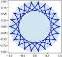
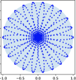
Refer to caption
Refer to caption
Refer to caption
Refer to caption
Refer to caption
Refer to caption
Refer to caption
Refer to caption
Refer to caption
Refer to caption
Refer to caption
Refer to caption
Refer to caption
Refer to caption
Refer to caption
Figure 4. Spectra of ΓN,εsuperscriptΓ𝑁𝜀\Gamma^{N,\varepsilon} for the circle shift map with θ=1π𝜃1𝜋\theta=\frac{1}{\pi} using N=1000𝑁1000N=1000 points, for ε{105,104,103,102,101}𝜀superscript105superscript104superscript103superscript102superscript101\varepsilon\in\{10^{-5},10^{-4},10^{-3},10^{-2},10^{-1}\} (left to right) and two different choices of the discretization: Upper row: points on a regular lattice; center row: points chosen randomly from a uniform distribution. In the center row, each plot shows the spectra for 100 realisations of the discretization points. For comparison, we show the eigenvalue asymptotics from Proposition 3 for ε3{107,106,105,104,103}𝜀3superscript107superscript106superscript105superscript104superscript103\varepsilon\in 3\cdot\{10^{-7},10^{-6},10^{-5},10^{-4},10^{-3}\} (left to right) in the lower row.

6.2. The Lorenz system

For a second experiment, we consider the classical Lorenz system [35]

u˙˙𝑢\displaystyle\dot{u} =σ(vu)absent𝜎𝑣𝑢\displaystyle=\sigma(v-u)
v˙˙𝑣\displaystyle\dot{v} =u(ρw)vabsent𝑢𝜌𝑤𝑣\displaystyle=u(\rho-w)-v
w˙˙𝑤\displaystyle\dot{w} =uvβwabsent𝑢𝑣𝛽𝑤\displaystyle=uv-\beta w

with parameter values σ=10,ρ=28,β=8/3formulae-sequence𝜎10formulae-sequence𝜌28𝛽83\sigma=10,\rho=28,\beta=8/3. The system possesses a robust strange attractor [47] which can be decomposed into several almost invariant sets [18]. We approximate the attractor by a point cloud x1N,,xNNsuperscriptsubscript𝑥1𝑁subscriptsuperscript𝑥𝑁𝑁x_{1}^{N},\ldots,x^{N}_{N} resulting from an equidistant sampling of the trajectory X=(u,v,w):[200,2000]3:𝑋𝑢𝑣𝑤2002000superscript3X=(u,v,w):[200,2000]\to{\mathbb{R}}^{3} with initial value X(0)=(1,1,1)𝑋0111X(0)=(1,1,1). The map F𝐹F is the flow map Fτsuperscript𝐹𝜏F^{\tau} with τ=0.1𝜏0.1\tau=0.1.

Refer to caption
Refer to caption
Figure 5. Largest real eigenvalues of ΓN,εsuperscriptΓ𝑁𝜀\Gamma^{N,\varepsilon} with N=1000𝑁1000N=1000 (left) and N=2000𝑁2000N=2000 (right) as a function of ε𝜀\varepsilon for the Lorenz system.
Refer to caption
Refer to caption
Figure 6. Eigenvectors at λ1subscript𝜆1\lambda_{1} (left) and λ2subscript𝜆2\lambda_{2} (right) of ΓN,εsuperscriptΓ𝑁𝜀\Gamma^{N,\varepsilon} with N=2000𝑁2000N=2000 and ε=10𝜀10\varepsilon=10 for the Lorenz system.

The largest real eigenvalues of ΓN,εsuperscriptΓ𝑁𝜀\Gamma^{N,\varepsilon} for N=1000𝑁1000N=1000 and N=2000𝑁2000N=2000 are shown in Figure 5 as a function of ε𝜀\varepsilon. For both values of N𝑁N, there are two real eigenvalues λ1,λ2<1subscript𝜆1subscript𝜆21\lambda_{1},\lambda_{2}<1 that decay much slower with increasing ε𝜀\varepsilon than the other eigenvalues. The corresponding eigenvectors each give rise to a decomposition of the point cloud into two almost invariant sets via their sign structure as shown in Figure 6. This is in aggreement with previuous results on the Lorenz system in, e.g., [13, 18]. For N=2000𝑁2000N=2000 points, there is also a third eigenvalue λ3subscript𝜆3\lambda_{3} very close to 1 which quickly decays at ε1𝜀1\varepsilon\approx 1. It corresponds to a point xisubscript𝑥𝑖x_{i} near the origin where the point density is low and F(xi)xi𝐹subscript𝑥𝑖subscript𝑥𝑖F(x_{i})\approx x_{i}, such that for sufficiently small ε𝜀\varepsilon, mass at F(xi)𝐹subscript𝑥𝑖F(x_{i}) gets transported almost exclusively back to xisubscript𝑥𝑖x_{i}, thus forming a spurious invariant set that decays quickly as ε𝜀\sqrt{\varepsilon} reaches the scale of nearest neighbor distances around xisubscript𝑥𝑖x_{i}. Such isolated points become less likely as N𝑁N is increased and their eigenvectors can be identified easily.

6.3. Alanine dipeptide

As a third experiment we analyse the dynamics of alanine dipeptide, a small biomolecule which is often used as a non-trivial model system for the analysis of macroscopic dynamics, cf. for example [25]. Like in the Lorenz system, we use trajectory data, here on the positions of the heavy atoms as provided by [40, 52]333The data is available for download at https://markovmodel.github.io/mdshare/ALA2/.. The original time series results from time integration of the molecule over 250 ns with a time step of 1 ps, yielding M=250 000𝑀250000M=250\,000 points x^1,,x^Msubscript^𝑥1subscript^𝑥𝑀\hat{x}_{1},\ldots,\hat{x}_{M} in 30superscript30{\mathbb{R}}^{30}. Here, we subsample this trajectory and use only every 50th (resp. 25th) point, yielding a sequence x1N,,xNNsubscriptsuperscript𝑥𝑁1subscriptsuperscript𝑥𝑁𝑁x^{N}_{1},\ldots,x^{N}_{N}, N=5 000𝑁5000N=5\,000 (resp. 10 0001000010\,000), in 30superscript30{\mathbb{R}}^{30} which forms the data for our analysis. We define the map F𝐹F by time-delay, that is we let F(x^j):=x^j+10assign𝐹subscript^𝑥𝑗subscript^𝑥𝑗10F(\hat{x}_{j}):=\hat{x}_{j+10} for j=1,,M10𝑗1𝑀10j=1,\ldots,M-10. This time lag of 10 ps has been chosen experimentally such that the real spectrum of ΓN,εsuperscriptΓ𝑁𝜀\Gamma^{N,\varepsilon} is reasonably close to 1. We note, however, that the macroscopic structure of the eigenvectors, cf. Figure 9, remains the same for time lags between 1 ps and 30 ps while, of course, the spectrum changes.
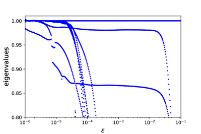
Refer to caption
Refer to caption
Figure 7. The 10 largest real eigenvalues of ΓN,εsuperscriptΓ𝑁𝜀\Gamma^{N,\varepsilon} as a function of ε𝜀\varepsilon for the alanine-dipeptide model for N=5000𝑁5000N=5000 (left) and N=10000𝑁10000N=10000 samples (right).

The left panel in Figure 7 shows the dominant real spectrum of ΓN,εsuperscriptΓ𝑁𝜀\Gamma^{N,\varepsilon} close to 111 as a function of ε𝜀\varepsilon for N=5000𝑁5000N=5000 and N=10000𝑁10000N=10000. There appear to be two eigenvalues λ10.98subscript𝜆10.98\lambda_{1}\approx 0.98 and λ20.87subscript𝜆20.87\lambda_{2}\approx 0.87 which are essentially constant over several orders of magnitude of ε𝜀\varepsilon. In fact, the corresponding eigenvectors give rise to the decomposition of the point cloud into three almost invariant sets as shown in Figure 9. There are several eigenvalues that are very close to one for ε[106,104.5]𝜀superscript106superscript104.5\varepsilon\in[10^{-6},10^{-4.5}] and that decay rapidly for ε[104.5,102]𝜀superscript104.5superscript102\varepsilon\in[10^{-4.5},10^{-2}]. In contrast, λ1subscript𝜆1\lambda_{1} and λ2subscript𝜆2\lambda_{2} do not decay for ε[104.5,102]𝜀superscript104.5superscript102\varepsilon\in[10^{-4.5},10^{-2}]. We conjecture that these correspond to spurious invariant subsets of the point cloud as described in the experiment on the Lorenz system.

In order to better understand the behaviour of the eigenvalues with increasing ε𝜀\varepsilon, we consider the simple Markov chain model with three states shown in Figure 8. We assume that the distance d1subscript𝑑1d_{1} between the states 2 and 3 is much (i.e. an order of magnitude) smaller than the distance d2subscript𝑑2d_{2} between 1 and 2 resp. 3. The transition matrix for this Markov chain is given by

T=[12p2p2p2p21p1p2p1p2p11p1p2].𝑇matrix12subscript𝑝2subscript𝑝2subscript𝑝2subscript𝑝21subscript𝑝1subscript𝑝2subscript𝑝1subscript𝑝2subscript𝑝11subscript𝑝1subscript𝑝2T=\begin{bmatrix}1-2p_{2}&p_{2}&p_{2}\\ p_{2}&1-p_{1}-p_{2}&p_{1}\\ p_{2}&p_{1}&1-p_{1}-p_{2}\end{bmatrix}.

Let Gε3×3superscript𝐺𝜀superscript33G^{\varepsilon}\in{\mathbb{R}}^{3\times 3} denote the matrix of the entropically regularized transport plan for the associated distance matrix

[0d2d2d20d1d2d10],matrix0subscript𝑑2subscript𝑑2subscript𝑑20subscript𝑑1subscript𝑑2subscript𝑑10\begin{bmatrix}0&d_{2}&d_{2}\\ d_{2}&0&d_{1}\\ d_{2}&d_{1}&0\end{bmatrix},

so that the entropically smoothed transfer operator is represented by the matrix Γε=GεTsuperscriptΓ𝜀superscript𝐺𝜀𝑇\Gamma^{\varepsilon}=G^{\varepsilon}T. There are two realms for ε𝜀\varepsilon for which the eigenvalues of ΓεsuperscriptΓ𝜀\Gamma^{\varepsilon} are essentially constant: For εd22much-less-than𝜀superscriptsubscript𝑑22\varepsilon\ll d_{2}^{2}, the smoothing has essentially no effect and the spectrum of ΓεsuperscriptΓ𝜀\Gamma^{\varepsilon} approximately coincides with that of T𝑇T itself. For εd22𝜀superscriptsubscript𝑑22\varepsilon\approx d_{2}^{2}, the smoothing starts to have an effect on the 23232\leftrightarrow 3 transition so that the associated eigenvalue starts to drop. At εd12𝜀superscriptsubscript𝑑12\varepsilon\approx d_{1}^{2}, also the 1{2,3}1231\leftrightarrow\{2,3\} transition is affected and the second real eigenvalue close to 1 starts to drop as well.
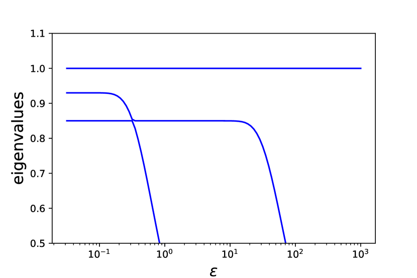
11122233312p212subscript𝑝21-2p_{2}1p1p21subscript𝑝1subscript𝑝21-p_{1}-p_{2}1p1p21subscript𝑝1subscript𝑝21-p_{1}-p_{2}p2subscript𝑝2p_{2}p2subscript𝑝2p_{2}p1subscript𝑝1p_{1}d2subscript𝑑2d_{2}d1subscript𝑑1d_{1}
Refer to caption
Figure 8. Simple Markov model showing the qualitative behaviour of the spectrum in Figure 7 for p1=0.01subscript𝑝10.01p_{1}=0.01, p2=0.05subscript𝑝20.05p_{2}=0.05, d1=1subscript𝑑11d_{1}=1, d2=10subscript𝑑210d_{2}=10.

Let us now return to the alanine dipeptide molecule. In Figure 9, we show the eigenvectors at λ10.98subscript𝜆10.98\lambda_{1}\approx 0.98 and λ20.86subscript𝜆20.86\lambda_{2}\approx 0.86 for different values of ε𝜀\varepsilon, projected onto the two relevant dihedral angles of the molecule. A k-means clustering of these (for ε=0.01𝜀0.01\varepsilon=0.01) yields the three almost invariant (a.k.a. metastable) sets shown in Figure 10 which correspond to the well-known dominant conformations of the molecule, cf. [25]. We stress the fact that we do not use any prior information on the dihedral angles in the computation but merely the raw trajectory data as described above. The angles are only used for the visualization of the eigenfunctions.

Refer to caption
Refer to caption
Refer to caption
Refer to caption
Refer to caption
Refer to caption
Refer to caption
Refer to caption
Figure 9. Projections of the eigenvectors of ΓN,εsuperscriptΓ𝑁𝜀\Gamma^{N,\varepsilon} for the alanine dipeptide model at λ10.98subscript𝜆10.98\lambda_{1}\approx 0.98 (upper row) and λ20.86subscript𝜆20.86\lambda_{2}\approx 0.86 (lower row) for N=5000𝑁5000N=5000 and ε=3105,104,103,102𝜀3superscript105superscript104superscript103superscript102\varepsilon=3\cdot 10^{-5},10^{-4},10^{-3},10^{-2} (from left to right).
Refer to caption
Refer to caption
Refer to caption
Figure 10. Projections of almost invariant sets as resulting from a k-means clustering of the two eigenvectors show in Figure 9 for ε=0.01𝜀0.01\varepsilon=0.01.

7. Comparison to other methods

We give a brief comparison to related data-based methods for approximating the transfer operator.

7.1. Normalized (conditional) Gaussian kernel

In [19], a data-based approximation of T𝑇T was proposed which is related to our approach (the same normalization has also been used in [28]). There, a regularized transfer operator Tε:L2(μ)L2(μ):superscript𝑇𝜀superscript𝐿2𝜇superscript𝐿2𝜇T^{\varepsilon}:L^{2}(\mu)\to L^{2}(\mu) also takes the form (cf. Section 4.2)

(59) (Tεh)(y)superscript𝑇𝜀𝑦\displaystyle(T^{\varepsilon}h)(y) :=𝒳tε(x,y)h(x)dμ(x),assignabsentsubscript𝒳superscript𝑡𝜀𝑥𝑦𝑥differential-d𝜇𝑥\displaystyle:=\int_{\mathcal{X}}t^{\varepsilon}(x,y)\,h(x)\;\mathrm{d}\mu(x), tε(x,y)superscript𝑡𝜀𝑥𝑦\displaystyle t^{\varepsilon}(x,y) :=1C(x)exp(c(F(x),y)ε)assignabsent1𝐶𝑥𝑐𝐹𝑥𝑦𝜀\displaystyle:=\frac{1}{C(x)}\exp\left(\frac{-c(F(x),y)}{\varepsilon}\right)

with C(x):=exp(c(F(x),y)/ε)dμ(y)assign𝐶𝑥𝑐𝐹𝑥𝑦𝜀differential-d𝜇𝑦C(x):=\int\exp(-c(F(x),y)/\varepsilon)\;\mathrm{d}\mu(y). The kernel tε(x,)superscript𝑡𝜀𝑥t^{\varepsilon}(x,\cdot) is a conditional Gaussian kernel, normalized such that tε(x,y)dμ(y)=1superscript𝑡𝜀𝑥𝑦differential-d𝜇𝑦1\int t^{\varepsilon}(x,y)\;\mathrm{d}\mu(y)=1 for μ𝜇\mu-a.e. x𝑥x. It becomes equal to (23) and (24) for the particular choice exp(α(F(x))/ε)=1/C(x)𝛼𝐹𝑥𝜀1𝐶𝑥\exp(\alpha(F(x))/\varepsilon)=1/C(x) and β(y)=0𝛽𝑦0\beta(y)=0, which corresponds to initializing α(F(x))=β(y)=0𝛼𝐹𝑥𝛽𝑦0\alpha(F(x))=\beta(y)=0 and running a single α𝛼\alpha-half-iteration of the Sinkhorn algorithm (18). Like in our approach, the discretized operator TN,εsuperscript𝑇𝑁𝜀T^{N,\varepsilon} results from approximating μ𝜇\mu by the empirical measure μNsuperscript𝜇𝑁\mu^{N} supported on the data points.

The dominating real spectrum of (59) for the Lorenz system is shown in Figure 11 (left). For large ε𝜀\varepsilon it is qualitatively similar to that of the entropic transfer operator. Only applying a single Sinkhorn half-iteration means that in general one has

tε(x,y)dμ(x)1superscript𝑡𝜀𝑥𝑦differential-d𝜇𝑥1\int t^{\varepsilon}(x,y)\;\mathrm{d}\mu(x)\neq 1

and thus the constant density h:x1L2(μ):maps-to𝑥1superscript𝐿2𝜇h:x\mapsto 1\in L^{2}(\mu) is generally not a fixed point of Tεsuperscript𝑇𝜀T^{\varepsilon}. So this smoothing procedure perturbs the invariant measure of the operator. This also holds for the discrete approximation TN,εsuperscript𝑇𝑁𝜀T^{N,\varepsilon}, as shown in Figure 12. Indeed, the stationary density exhibits substantial fluctuations and several local spurious spikes.
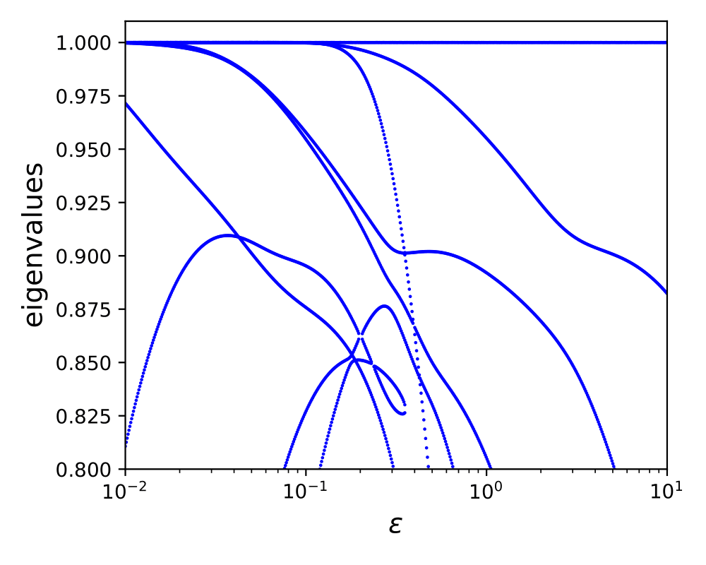
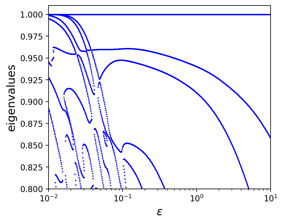
Refer to caption
Refer to caption
Figure 11. Real spectrum of TN,εsuperscript𝑇𝑁𝜀T^{N,\varepsilon} with N=1000𝑁1000N=1000 as a function of ε𝜀\varepsilon for the Lorenz system using the construction in (59) from [19] (left), and using the entropic transfer operator (right, identical to the left panel in Figure 5).
Refer to caption
Refer to caption
Figure 12. Stationary density of TN,εsuperscript𝑇𝑁𝜀T^{N,\varepsilon} with N=2000𝑁2000N=2000, ε=10𝜀10\varepsilon=10 using the construction (59) from [19] (left) and using the entropic transfer operator (right). Note that the density on the left is not constant while the one on the right is.

7.2. Extended dynamic mode decomposition

Secondly, we compare our approach to extended dynamic mode decomposition (EDMD) [43, 53], which is a prominent data based scheme for approximation of the Koopman operator. Let ψ1,,ψJsubscript𝜓1subscript𝜓𝐽\psi_{1},\ldots,\psi_{J} be a dictionary of functions in C(𝒳)𝐶𝒳C(\mathcal{X}). In EDMD, one seeks an approximation KNsuperscript𝐾𝑁K^{N} of K𝐾K on span(ψj)jspansubscriptsubscript𝜓𝑗𝑗\mathrm{span}(\psi_{j})_{j} by enforcing the conditions

(60) ψj(F(xiN))=(Kψj)(xiN),i=1,,N,j=1,,J,formulae-sequencesubscript𝜓𝑗𝐹subscriptsuperscript𝑥𝑁𝑖𝐾subscript𝜓𝑗subscriptsuperscript𝑥𝑁𝑖formulae-sequence𝑖1𝑁𝑗1𝐽\displaystyle\psi_{j}(F(x^{N}_{i}))=(K\psi_{j})(x^{N}_{i}),\quad i=1,\ldots,N,\ j=1,\ldots,J,

in a least squares sense: define rectangular matrices A,BN×J𝐴𝐵superscript𝑁𝐽A,B\in{\mathbb{R}}^{N\times J} by Ai,j=ψj(xiN)subscript𝐴𝑖𝑗subscript𝜓𝑗superscriptsubscript𝑥𝑖𝑁A_{i,j}=\psi_{j}(x_{i}^{N}) and Bi,j=ψj(F(xiN))subscript𝐵𝑖𝑗subscript𝜓𝑗𝐹superscriptsubscript𝑥𝑖𝑁B_{i,j}=\psi_{j}(F(x_{i}^{N})), and minimize the Frobenius norm

(61) BAKNF2superscriptsubscriptnorm𝐵𝐴superscript𝐾𝑁𝐹2\|B-AK^{N}\|_{F}^{2}

among all KNJ×Jsuperscript𝐾𝑁superscript𝐽𝐽K^{N}\in{\mathbb{R}}^{J\times J}. A least squares loss is preferable since the system (60) is often overdetermined (NJmuch-greater-than𝑁𝐽N\gg J), the evaluations of F𝐹F might be subject to noise, and invariance of span(ψj)jspansubscriptsubscript𝜓𝑗𝑗\mathrm{span}(\psi_{j})_{j} under K𝐾K cannot be expected in general. The solution of (61) is given in terms of A𝐴A’s pseudo-inverse A+superscript𝐴A^{+},

KN=A+B.superscript𝐾𝑁superscript𝐴𝐵K^{N}=A^{+}B.

The choice of the dictionary (ψj)jsubscriptsubscript𝜓𝑗𝑗(\psi_{j})_{j} determines how well the spectrum of KNsuperscript𝐾𝑁K^{N} approximates that of K𝐾K. In the absence of prior information on the eigenvectors of K𝐾K, a popular choice for the dictionary are radial functions centered at the sample points (xiN)isubscriptsuperscriptsubscript𝑥𝑖𝑁𝑖(x_{i}^{N})_{i}. In this case, J=N𝐽𝑁J=N, and A𝐴A is symmetric. Since A𝐴A is a square matrix, the minimizer in (61) can be approximated in a numerically robust way using the modified definition of A𝐴A by Ai,j=ψj(xiN)+σδi,jsubscript𝐴𝑖𝑗subscript𝜓𝑗superscriptsubscript𝑥𝑖𝑁𝜎subscript𝛿𝑖𝑗A_{i,j}=\psi_{j}(x_{i}^{N})+\sigma\delta_{i,j} for some (typically small) regularization σ>0𝜎0\sigma>0.

In our numerical experiments, we have chosen radial Gaussians,

(62) ψj(x):=ψjε(x):=exp(c(xjN,x)ε).assignsubscript𝜓𝑗𝑥subscriptsuperscript𝜓𝜀𝑗𝑥assign𝑐superscriptsubscript𝑥𝑗𝑁𝑥𝜀\displaystyle\psi_{j}(x):=\psi^{\varepsilon}_{j}(x):=\exp\left(-\frac{c(x_{j}^{N},x)}{\varepsilon}\right).

We denote the resulting approximation of K𝐾K by KN,εsuperscript𝐾𝑁𝜀K^{N,\varepsilon}. Then, TN,ε:=A+Bassignsuperscript𝑇𝑁𝜀superscript𝐴superscript𝐵topT^{N,\varepsilon}:=A^{+}B^{\top} is a corresponding approximation of T𝑇T on span(δxiN)ispansubscriptsubscript𝛿superscriptsubscript𝑥𝑖𝑁𝑖\mathrm{span}(\delta_{x_{i}^{N}})_{i}. This particular choice of dictionary can also be related to the famous kernel trick [54]. For the regularization parameter σ𝜎\sigma, we had to choose the rather large value σ=0.1𝜎0.1\sigma=0.1 in order to stabilize the computation: for smaller σ𝜎\sigma, some spectra were not contained in the unit circle anymore and their dependence on ε𝜀\varepsilon was not numerically stable.

Refer to caption
Refer to caption
Figure 13. Left: the largest real eigenvalues of KN,εsuperscript𝐾𝑁𝜀K^{N,\varepsilon} constructed via EDMD for the Lorenz system with N=1000𝑁1000N=1000 points as a function of ε𝜀\varepsilon. Right: the i𝑖i-th column of the matrix A+Bsuperscript𝐴superscript𝐵topA^{+}B^{\top} (cf. the main text), plotted in color over the point cloud (xjN)jsubscriptsuperscriptsubscript𝑥𝑗𝑁𝑗(x_{j}^{N})_{j}. Note that this column contains negative entries and that thus A+Bsuperscript𝐴superscript𝐵topA^{+}B^{\top} is not a Markov matrix.

The results of our numerical experiments are given in Figure 13. The left panel shows the largest real eigenvalues of TN,εsuperscript𝑇𝑁𝜀T^{N,\varepsilon} for N=1000𝑁1000N=1000 as a function of ε𝜀\varepsilon. In an intermediate range of ε𝜀\varepsilon, the dominating real eigenvalues of TN,εsuperscript𝑇𝑁𝜀T^{N,\varepsilon} (and the corresponding eigenvectors) encode qualitatively similar almost-invariant structures as the entropic transfer operator, cf. Section 4, although for different values of ε𝜀\varepsilon. The figure in the right panel illustrates a disadvantage of EDMD: the operators KN,εsuperscript𝐾𝑁𝜀K^{N,\varepsilon} and TN,εsuperscript𝑇𝑁𝜀T^{N,\varepsilon} are no longer Markov operators, i.e. one loses the interpretation of jump probabilities between samples.

There is a significant formal similarity between EDMD and our approach: for our choice of Gaussian radial basis functions in (62), the operator GN,εsuperscript𝐺𝑁𝜀G^{N,\varepsilon} is obtained by a row- and column-wise rescaling of the corresponding matrix B𝐵B through the dual variables α𝛼\alpha and β𝛽\beta (see (17) and Section 4). However, the role played by ε𝜀\varepsilon in EDMD is a slightly different one. There is no blur on the length scale ε1/2superscript𝜀12\varepsilon^{1/2} in KN,εsuperscript𝐾𝑁𝜀K^{N,\varepsilon} as for entropic transfer operators. The damping of eigenvalues in KN,εsuperscript𝐾𝑁𝜀K^{N,\varepsilon} depends on a more complex interplay between ε𝜀\varepsilon, N𝑁N and the inversion regularization weight σ𝜎\sigma. For example, for F(x)=x𝐹𝑥𝑥F(x)=x and σ=0𝜎0\sigma=0, one finds that A=B𝐴𝐵A=B and thus KN,εsuperscript𝐾𝑁𝜀K^{N,\varepsilon} is the identity operator on the span of the ψjsubscript𝜓𝑗\psi_{j}, independently of the value of ε𝜀\varepsilon. Also, the asymptotics in EDMD for small and large values of ε𝜀\varepsilon are different than for entropic transport: as ε𝜀\varepsilon\to\infty, all basis functions become increasingly aligned, i.e. Ai,j1subscript𝐴𝑖𝑗1A_{i,j}\to 1 and Bi,j1subscript𝐵𝑖𝑗1B_{i,j}\to 1 for all i,j𝑖𝑗i,j, which implies that all eigenvalues of A+Bsuperscript𝐴𝐵A^{+}B approach zero, except for one, which tends to 111 for the eigenvector with all entries one. For ε0𝜀0\varepsilon\to 0, we have Bi,j0subscript𝐵𝑖𝑗0B_{i,j}\to 0 in the generic case where xiNF(xjN)subscriptsuperscript𝑥𝑁𝑖𝐹subscriptsuperscript𝑥𝑁𝑗x^{N}_{i}\neq F(x^{N}_{j}) for all i,j𝑖𝑗i,j, whereas A+superscript𝐴A^{+} remains bounded, and so all eigenvalues of KN,εsuperscript𝐾𝑁𝜀K^{N,\varepsilon} approach zero.

7.3. Diffusion maps

Another conceptually related method are diffusion maps [9]. On a pair (𝒳,μ)𝒳𝜇(\mathcal{X},\mu) one defines a Markov operator Tεsuperscript𝑇𝜀T^{\varepsilon} via its kernel

tε(x,y):=1C(x)exp(c(x,y)ε)assignsuperscript𝑡𝜀𝑥𝑦1𝐶𝑥𝑐𝑥𝑦𝜀t^{\varepsilon}(x,y):=\frac{1}{C(x)}\exp\left(\frac{-c(x,y)}{\varepsilon}\right)

with C(x):=exp(c(x,y)/ε)dμ(y)assign𝐶𝑥𝑐𝑥𝑦𝜀differential-d𝜇𝑦C(x):=\int\exp(-c(x,y)/\varepsilon)\;\mathrm{d}\mu(y). As above, TN,εsuperscript𝑇𝑁𝜀T^{N,\varepsilon} can be approximated by using μNsuperscript𝜇𝑁\mu^{N} as substitute for μ𝜇\mu. Note that this operator does not explicitely incorporate the map F𝐹F, and thus its spectrum contains no direct information on the dynamics. Implicitly, the invariant measure μ𝜇\mu may of course depend on F𝐹F. Instead, the specturm of this Tεsuperscript𝑇𝜀T^{\varepsilon} contains information about the distribution of μ𝜇\mu and its dominant eigenfunctions can be used to obtain a lower-dimensional embedding of (𝒳,μ)𝒳𝜇(\mathcal{X},\mu). On this embedding one may then apply Ulam’s method, which may be unfeasible on the original high-dimensional dynamics, see for instance [30]. In comparison, the method of Section 7.1 and entropic transfer operators can be interpreted as mesh-free versions of Ulam’s method that do not require a separate dimensionality reduction.

In [46] it is proposed to estimate the metric d𝑑d (which induces the cost c=d2𝑐superscript𝑑2c=d^{2}) for the definition of tεsuperscript𝑡𝜀t^{\varepsilon} from the local diffusivity of a stochastic dynamical system, thus assigning higher emphasis on ‘slow’ coordinates in the subsequent low-dimensional embedding. While stochastic systems are beyond the scope of the present paper, if such a relevant data-driven metric d𝑑d were available it could potentially also be used in the definition of the entropic transfer operator.

8. Conclusion

In this article we have introduced a new method for the regularization, discretization and numerical spectral analysis of transfer operators by using entropic optimal transport. The analysis of the torus shift map and the numerical experiments indicate that this might be a promising avenue to follow.

Due to its Lagrangian nature, the method is readily applicable to problems with high-dimensional dynamics, in contrast to grid- or set-oriented methods, since no explicit covering of the support of the invariant measure μ𝜇\mu needs to be constructed. However, the performance of the numerical method depends on whether the discretization captures the features of interest. The results in Section 5 give a first impression on how “feature size”, discretization scale and blur scale may be intertwined. Clearly, features below the blur scale will not be uncovered. On the other hand, the blur scale needs to be above the discretization scale since otherwise the discrete transfer operator approximation degenerates to a permutation matrix.

A better analytical understanding between the three scales beyond the shift map on the torus would therefore be a relevant open question. For example, the invariant measure in the torus example has full support and thus the required relation between N𝑁N and ε𝜀\varepsilon was given by N=ndεd/2𝑁superscript𝑛𝑑much-greater-thansuperscript𝜀𝑑2N=n^{d}\gg\varepsilon^{-d/2}, i.e. the required number of points to resolve a given blur scale increases exponentially with d𝑑d, the so-called curse of dimensionality. In other cases, when the dimension of the support of μ𝜇\mu is lower than the dimension of 𝒳𝒳\mathcal{X}, it seems plausible that N𝑁N scales based on the dimension of the former, not the latter, as suggested by the alanine dipeptide example in d=30𝑑30d=30. Can this be established rigorously? We refer to [51, 38, 22] for related results. When the number N𝑁N of points is small, can we still expect to reliably recover features at least on coarse scales? These questions may be related to the improved sample complexity of entropic optimal transport as compared to the unregularized version [20]. Such results would confirm that our method can extract some spectral information even from coarse approximations of μ𝜇\mu, as indicated by some of the numerical experiments.

While here we formulated our approach for an underlying deterministic map, an application to a stochastic model is straightforward: The original transfer operator T𝑇T will then be defined directly in terms of a stochastic transition function, it can again be combined with entropic smoothing. In fact, computationally a single realization of some random trajectory of the stochastic model might already be sufficient, if it samples the support of the invariant measure well enough.

9. Acknowledgments

This research was supported by the DFG Collaborative Research Center TRR 109, “Discretization in Geometry and Dynamics”. BS was supported by the Emmy Noether Programme of the DFG (project number 403056140).

References

  • [1] L. Ambrosio, N. Gigli, and G. Savaré. Gradient Flows in Metric Spaces and in the Space of Probability Measures. Lectures in Mathematics. Birkhäuser Boston, 2nd edition, 2008.
  • [2] C. Bose and R. Murray. The exact rate of approximation in Ulam’s method. Discrete Contin. Dynam. Systems, 7(1):219–235, 2001.
  • [3] J. H. Bramble and J. Osborn. Rate of convergence estimates for nonselfadjoint eigenvalue approximations. Mathematics of computation, 27(123):525–549, 1973.
  • [4] Y. Brenier. Polar factorization and monotone rearrangement of vector-valued functions. Comm. Pure Appl. Math., 44(4):375–417, 1991.
  • [5] M. Budišić, R. Mohr, and I. Mezić. Applied Koopmanism. Chaos: An Interdisciplinary Journal of Nonlinear Science, 22(4):047510, 2012.
  • [6] T. Cai, J. Cheng, B. Schmitzer, and M. Thorpe. The linearized Hellinger–Kantorovich distance. SIAM J. Imaging Sci., 15(1):45–83, 2022.
  • [7] G. Carlier, V. Duval, G. Peyré, and B. Schmitzer. Convergence of entropic schemes for optimal transport and gradient flows. SIAM J. Math. Anal., 49(2):1385–1418, 2017.
  • [8] B. Charlier, J. Feydy, J. A. Glaunès, F.-D. Collin, and G. Durif. Kernel operations on the GPU, with autodiff, without memory overflows. Journal of Machine Learning Research, 22(74):1–6, 2021.
  • [9] R. R. Coifman and S. Lafon. Diffusion maps. Appl. Comput. Harmon. Anal., 21(1):5–30, 2006.
  • [10] D. Crommelin and E. Vanden-Eijnden. Reconstruction of diffusions using spectral data from timeseries. Communications in Mathematical Sciences, 4(3):651–668, 2006.
  • [11] M. Cuturi. Sinkhorn distances: Lightspeed computation of optimal transport. Advances in neural information processing systems, 26:2292–2300, 2013.
  • [12] M. Dellnitz and A. Hohmann. A subdivision algorithm for the computation of unstable manifolds and global attractors. Numer. Math., 75(3):293–317, 1997.
  • [13] M. Dellnitz and O. Junge. On the approximation of complicated dynamical behavior. SIAM J. Numer. Anal., 36(2):491–515, 1999.
  • [14] J. Ding and A. Zhou. The projection method for a class of Frobenius-Perron operators. Applied mathematics letters, 12(1):71–74, 1999.
  • [15] J. Feydy. Geometric data analysis, beyond convolutions. PhD thesis, Universit’e Paris-Saclay, 2020.
  • [16] J. Feydy, T. Séjourné, F.-X. Vialard, S.-i. Amari, A. Trouve, and G. Peyré. Interpolating between optimal transport and mmd using sinkhorn divergences. In The 22nd International Conference on Artificial Intelligence and Statistics, pages 2681–2690, 2019.
  • [17] G. Froyland. An analytic framework for identifying finite-time coherent sets in time-dependent dynamical systems. Physica D, 250:1–19, 2013.
  • [18] G. Froyland and M. Dellnitz. Detecting and locating near-optimal almost-invariant sets and cycles. SIAM Journal on Scientific Computing, 24(6):1839–1863, 2003.
  • [19] G. Froyland, D. Giannakis, B. R. Lintner, M. Pike, and J. Slawinska. Spectral analysis of climate dynamics with operator-theoretic approaches. Nature communications, 12(1):6570, 2021.
  • [20] A. Genevay, L. Chizat, F. Bach, M. Cuturi, and G. Peyré. Sample complexity of Sinkhorn divergences. In K. Chaudhuri and M. Sugiyama, editors, Proceedings of Machine Learning Research, volume 89, pages 1574–1583, 2019.
  • [21] C. S. Hsu. A generalized theory of cell-to-cell mapping for nonlinear dynamical systems. Trans. ASME Ser. E. J. Appl. Mech., 48(3):634–642, 1981.
  • [22] S. Hundrieser, T. Staudt, and A. Munk. Empirical optimal transport between different measures adapts to lower complexity. arXiv:2202.10434, 2022.
  • [23] F. Y. Hunt. Unique ergodicity and the approximation of attractors and their invariant measures using Ulam’s method. Nonlinearity, 11(2):307–317, 1998.
  • [24] Y. Kifer. Random perturbations of dynamical systems, volume 16 of Prog. Probab. Stat. Boston, MA: Birkhäuser Verlag, 1988.
  • [25] S. Klus, A. Bittracher, I. Schuster, and C. Schütte. A kernel-based approach to molecular conformation analysis. The Journal of chemical physics, 149(24):244109, 2018.
  • [26] S. Klus, P. Koltai, and C. Schütte. On the numerical approximation of the Perron-Frobenius and Koopman operator. Journal of Computational Dynamics, 3(1):51, 2016.
  • [27] S. Klus, F. Nüske, S. Peitz, J.-H. Niemann, C. Clementi, and C. Schütte. Data-driven approximation of the koopman generator: Model reduction, system identification, and control. Physica D: Nonlinear Phenomena, 406:132416, 2020.
  • [28] P. Koltai and D. R. M. Renger. From large deviations to semidistances of transport and mixing: coherence analysis for finite Lagrangian data. J Nonlinear Sci, 28:1915–1957, 2018.
  • [29] P. Koltai, J. von Lindheim, S. Neumayer, and G. Steidl. Transfer operators from optimal transport plans for coherent set detection. Physica D, 426:132980, 2021.
  • [30] P. Koltai and S. Weiss. Diffusion maps embedding and transition matrix analysis of the large-scale flow structure in turbulent Rayleigh–Bénard convection. Nonlinearity, 33(4):1723, 2020.
  • [31] B. O. Koopman. Hamiltonian systems and transformations in Hilbert space. Proc. Natl. Acad. Sci. USA, 17:315–318, 1931.
  • [32] A. Lasota and M. C. Mackey. Chaos, fractals, and noise: stochastic aspects of dynamics, volume 97. Springer Science & Business Media, 2013.
  • [33] A. Lasota and J. A. Yorke. On the existence of invariant measures for piecewise monotonic transformations. Trans. Am. Math. Soc., 186:481–488, 1974.
  • [34] T.-Y. Li. Finite approximation for the Frobenius-Perron operator. A solution to Ulam’s conjecture. Journal of Approximation theory, 17(2):177–186, 1976.
  • [35] E. N. Lorenz. Deterministic nonperiodic flow. Journal of atmospheric sciences, 20(2):130–141, 1963.
  • [36] I. Mezić. Spectral properties of dynamical systems, model reduction and decompositions. Nonlinear Dynamics, 41:309–325, 2005.
  • [37] G. Monge. Mémoire sur la thèorie des déblais et des remblais. Histoire de l’Académie royale des sciences avec les mémoires de mathématique et de physique tirés des registres de cette Académie, pages 666–705, 1781.
  • [38] J. Niles-Weed and P. Rigollet. Estimation of Wasserstein distances in the spiked transport model. Bernoulli, 28(4):2663–2688, 2022.
  • [39] F. Nüske, L. Boninsegna, and C. Clementi. Coarse-graining molecular systems by spectral matching. The Journal of chemical physics, 151(4), 2019.
  • [40] F. Nüske, H. Wu, J.-H. Prinz, C. Wehmeyer, C. Clementi, and F. Noé. Markov state models from short non-equilibrium simulations—analysis and correction of estimation bias. The Journal of Chemical Physics, 146(9):094104, 2017.
  • [41] J. E. Osborn. Spectral approximation for compact operators. Mathematics of computation, 29(131):712–725, 1975.
  • [42] G. Peyré and M. Cuturi. Computational optimal transport. Foundations and Trends in Machine Learning, 11(5–6):355–607, 2019.
  • [43] C. W. Rowley, I. Mezić, S. Bagheri, P. Schlatter, and D. S. Henningson. Spectral analysis of nonlinear flows. Journal of fluid mechanics, 641:115–127, 2009.
  • [44] F. Santambrogio. Optimal Transport for Applied Mathematicians, volume 87 of Progress in Nonlinear Differential Equations and Their Applications. Birkhäuser Boston, 2015.
  • [45] B. Schmitzer. Stabilized sparse scaling algorithms for entropy regularized transport problems. SIAM J. Sci. Comput., 41(3):A1443–A1481, 2019.
  • [46] A. Singer, R. Erban, I. G. Kevrekidis, and R. R. Coifman. Detecting intrinsic slow variables in stochastic dynamical systems by anisotropic diffusion maps. Proceedings of the National Academy of Sciences, 106(38):16090–16095, 2009.
  • [47] W. Tucker. The Lorenz attractor exists. Comptes Rendus de l’Académie des Sciences-Series I-Mathematics, 328(12):1197–1202, 1999.
  • [48] S. M. Ulam. A collection of mathematical problems. Interscience Tracts in Pure and Applied Mathematics, no. 8. Interscience Publishers, New York-London, 1960.
  • [49] C. Villani. Optimal Transport: Old and New, volume 338 of Grundlehren der mathematischen Wissenschaften. Springer, 2009.
  • [50] J. von Neumann. Proof of the quasi-ergodic hypothesis. Proc. Natl. Acad. Sci. USA, 18:70–82, 1932.
  • [51] J. Weed and F. Bach. Sharp asymptotic and finite-sample rates of convergence ofempirical measures in Wasserstein distance. Bernoulli, 25(4A):2620–2648, 2019.
  • [52] C. Wehmeyer and F. Noé. Time-lagged autoencoders: Deep learning of slow collective variables for molecular kinetics. The Journal of chemical physics, 148(24):241703, 2018.
  • [53] M. O. Williams, I. G. Kevrekidis, and C. W. Rowley. A data–driven approximation of the Koopman operator: Extending dynamic mode decomposition. Journal of Nonlinear Science, 25(6):1307–1346, 2015.
  • [54] M. O. Williams, C. W. Rowley, and I. G. Kevrekidis. A kernel-based method for data-driven Koopman spectral analysis. Journal of Computational Dynamics, 2(2):247–265, 2016.
  • [55] K. Yosida. Functional analysis. 6th ed, volume 123 of Grundlehren Math. Wiss. Springer, Cham, 1980.