Local volatility under rough volatility

F. Bourgey florian.bourgey@polytechnique.edu Centre de Mathématiques Appliquées (CMAP), CNRS, Ecole Polytechnique, Institut Polytechnique de Paris, France Bloomberg L.P., Quantitative Research, London, UK S. De Marco stefano.de-marco@polytechnique.edu Centre de Mathématiques Appliquées (CMAP), CNRS, Ecole Polytechnique, Institut Polytechnique de Paris, France P. K. Friz friz@math.tu-berlin.de Technische Universität Berlin and Weierstraß-Institut, Berlin, Germany P. Pigato paolo.pigato@uniroma2.it Department of Economics and Finance, Università Roma Tor Vergata, Rome, Italy
Abstract

Several asymptotic results for the implied volatility generated by a rough volatility model have been obtained in recent years (notably in the small-maturity regime), providing a better understanding of the shapes of the volatility surface induced by rough volatility models, supporting their calibration power to SP500 option data. Rough volatility models also generate a local volatility surface, via the so-called Markovian projection of the stochastic volatility. We complement the existing results on implied volatility by studying the asymptotic behavior of the local volatility surface generated by a class of rough stochastic volatility models, encompassing the rough Bergomi model. Notably, we observe that the celebrated “1/2121/2 skew rule” linking the short-term at-the-money skew of the implied volatility to the short-term at-the-money skew of the local volatility, a consequence of the celebrated “harmonic mean formula” of [Berestycki, Busca, and Florent, QF 2002], is replaced by a new rule: the ratio of the at-the-money implied and local volatility skews tends to the constant 1/(H+3/2)1𝐻321/(H+3/2) (as opposed to the constant 1/2121/2), where H𝐻H is the regularity index of the underlying instantaneous volatility process.

1 Introduction

In rough stochastic volatility models, volatility is driven by a fractional noise, in the rough regime of Hurst parameter H𝐻H less than 1/2. With no claim of completeness, we mention econometric evidence [45, 40, 15], market microstructure foundations [26], efficient numerical methods and simulations schemes [11, 14, 58, 27], including deep learning algorithms [13, 47].

This work is concerned with pricing under rough volatility, a key feature of which, well-adapted to the steep volatility skews seen in Equity option markets, is the power-law behavior of the short-dated implied volatility at-the-money (ATM) skew:

𝒮BS(const)tH1/2;similar-tosubscript𝒮BSconstsuperscript𝑡𝐻12\mathcal{S}_{\mathrm{BS}}\sim\mathrm{(const)}t^{H-1/2}\,;

references include [3, 37, 6, 8, 28, 25, 38, 32, 49, 39, 12]. More specifically, we consider here - to the best of our knowledge for the first time - the Dupire local volatility [24, 23] generated by rough volatility models, using a Gyongy-type projection [51, 18] and study its short-time behavior in a large deviations regime. In the context of implied volatility, such a regime was pioneered in [28], with instantaneous stochastic volatility process given as v(t,ω)=σ(WtH(ω))𝑣𝑡𝜔𝜎subscriptsuperscript𝑊𝐻𝑡𝜔v(t,\omega)=\sigma(W^{H}_{t}(\omega)), i.e., as some explicit function of a fractional Brownian motion (fBm). In particular, no rough or Volterra stochastic differential equations need to be solved. We shall work under the same structural assumption as [28], although under less restrictive growth assumptions, such as to include the popular rough Bergomi model [6] where σ𝜎\sigma has exponential form. Postponing detailed recalls and precise definitions, our main result (Theorem 3.3) states that,

σloc(t,yt1/2H)σ(h^1y) as t0,formulae-sequencesubscript𝜎loc𝑡𝑦superscript𝑡12𝐻𝜎superscriptsubscript^1𝑦 as 𝑡0\sigma_{\mathrm{loc}}\bigl{(}t,y\,t^{1/2-H}\bigr{)}\to\sigma\bigl{(}\,\widehat{h}_{1}^{y}\,\bigr{)}\quad\mbox{ as }t\downarrow 0,

where h^ysuperscript^𝑦\widehat{h}^{y} is related to a minimization problem, similar to a geodesic in Riemannian geometry. Our analytic understanding is sufficiently fine to exploit it on the one hand for numerical tests (discussed in Section 4) and on the other hand to derive further analytic results (formulated in Sections 2 and 3, with proofs left to Section 5) including the blowup, when H<1/2𝐻12H<1/2, of the local volatility skew in the short-dated limit,

𝒮loc(const)tH1/2,similar-tosubscript𝒮locconstsuperscript𝑡𝐻12\mathcal{S}_{\mathrm{loc}}\sim\mathrm{(const)}t^{H-1/2},

see Corollary 3.4 below for a precise statement and information on the constant. This finding is consistent with [38] where it is shown, amongst others, that in “regular” local-stochastic vol models, which amounts to a regularity assumption on σlocsubscript𝜎loc\sigma_{\mathrm{loc}}, the implied volatility skew does not explode. The regularity of σlocsubscript𝜎loc\sigma_{\mathrm{loc}} is violated here in the sense that 𝒮locsubscript𝒮loc\mathcal{S}_{\mathrm{loc}} is infinite at t=0𝑡0t=0. This is also consistent with [60, 36] where it is shown that a “singular” σlocsubscript𝜎loc\sigma_{\mathrm{loc}} can indeed produce exploding implied skews.

A further interesting consequence, also part of Corollary 3.4, is then that the 1/2121/2-rule of thumb from practitioners [22] (see also [43] and [39, Remark 3.4] for different proofs) actually fails and is replaced, again in the short-dated limit, by what we may call the 1/(H+3/2)1𝐻321/(H+3/2)-rule,

𝒮BS𝒮loc1H+3/2.subscript𝒮BSsubscript𝒮loc1𝐻32\frac{\mathcal{S}_{\mathrm{BS}}}{\mathcal{S}_{\mathrm{loc}}}\to\frac{1}{H+3/2}. (1.1)

As a sanity check, for Hurst parameter H=1/2𝐻12H=1/2 we are in a diffusive regime and then indeed fall back to the 1/2121/2-rule.

Techniques and further discussion. Our analysis is based on a mixture of large deviations (see e.g. [33] for a recent collection with many references), Malliavin calculus [5, 59, 29], and last not least ideas from rough paths and regularity structures techniques, following [7, 31, 32]; see also Section 14.6 in [35]. In order to deal with H<1/2𝐻12H<1/2, we cannot rely on previously used methods in diffusion settings such as [62, 21]. Local volatility in classical stochastic volatility models, including Heston, is discussed in many books on volatility modeling, [43] remains a key reference. Rigorous asymptotic results include [44, 20, 21]. In affine forward variance models, including rough Heston [27, 46], it is conceivable that saddle-point-based techniques, in the spirit of [20] could be employed to study local volatility asymptotics. The bottleneck in such an approach seems however the lack of explicit knowledge of the moment-generating function, only given implicitly via convolution Riccati equations. We note that the recent preprint [2] confirmed the asymptotic result (1.1) using some representations of 𝒮BSsubscript𝒮BS\mathcal{S}_{\mathrm{BS}} and 𝒮locsubscript𝒮loc\mathcal{S}_{\mathrm{loc}} based on Malliavin calculus, in a central limit (Edgeworth) regime, as opposed to our large deviations setting.

Acknowledgements: PKF gratefully acknowledges financial support from European Research Council (ERC) Grant CoG-683164 and German science foundation (DFG) via the cluster of excellence MATH+, project AA4-2. SDM gratefully acknowledges financial support from the research projects Chaire Risques Financiers (École Polytechnique, Fondation du Risque and Société Générale) and Chaire Stress Test, Risk Management and Financial Steering (École Polytechnique, Fondation de l’École Polytechnique and BNP Paribas). PP gratefully acknowledges financial support from INDAM-GNAMPA. We thank Martin Forde, Masaaki Fukasawa, Paul Gassiat, Antoine Jacquier, Fabio Mercurio, Olivier Pradère, Sergio Pulido, Adil Reghai, Mathieu Rosenbaum and Guillaume Sebille for feedback and stimulating discussions on the subject of this article, and Andrea Pallavicini and Riccardo Longoni for their inspiring comments and insights.

2 The modeling framework

We assume S0=1subscript𝑆01S_{0}=1 and that the log price Xt:=logStassignsubscript𝑋𝑡subscript𝑆𝑡X_{t}:=\log S_{t} satisfies

dXt=12Vtdt+Vt(ρdWt+ρ¯dW¯t)Vt=σ2(W^t)dsubscript𝑋𝑡12subscript𝑉𝑡d𝑡subscript𝑉𝑡𝜌dsubscript𝑊𝑡¯𝜌dsubscript¯𝑊𝑡subscript𝑉𝑡superscript𝜎2subscript^𝑊𝑡\begin{split}\mathrm{d}X_{t}&=-\frac{1}{2}V_{t}\mathrm{d}t+\sqrt{V_{t}}\left(\rho\,\mathrm{d}W_{t}+\overline{\rho}\,\mathrm{d}\overline{W}_{t}\right)\\ V_{t}&=\sigma^{2}(\widehat{W}_{t})\end{split} (2.1)

with ‘volatility function’ σ::𝜎\sigma:\mathbb{R}\to\mathbb{R}. We shall assume σ𝜎\sigma to be smooth, subject to mild growth conditions given below, such as to cover rough Bergomi type situations where σ(x)=σ0exp(ηx)𝜎𝑥subscript𝜎0𝜂𝑥\sigma(x)=\sigma_{0}\exp(\eta x).

Assumption 2.1.

There exist c1,c2,c3,c4>0subscript𝑐1subscript𝑐2subscript𝑐3subscript𝑐40c_{1},c_{2},c_{3},c_{4}>0 such that for all x𝑥x\in\mathbb{R},

c1ec2|x|subscript𝑐1superscript𝑒subscript𝑐2𝑥\displaystyle c_{1}e^{-c_{2}|x|} σ(x),absent𝜎𝑥\displaystyle\leq\sigma(x), (2.2)
σ(x)𝜎𝑥\displaystyle\sigma(x) c3ec4|x|.absentsubscript𝑐3superscript𝑒subscript𝑐4𝑥\displaystyle\leq c_{3}e^{c_{4}|x|}. (2.3)

We take ρ2+ρ¯2=1superscript𝜌2superscript¯𝜌21\rho^{2}+\overline{\rho}^{2}=1, with ρ(1,1)𝜌11\rho\in(-1,1). We denote W=(W,W¯)W𝑊¯𝑊\mathrm{W}=(W,\overline{W}) where W,W¯𝑊¯𝑊W,\overline{W} are two independent standard Brownian motions. These are used to construct

W~t=ρ¯W¯t+ρWtandW^t=(KW˙)t=0tK(t,s)dWs,formulae-sequencesubscript~𝑊𝑡¯𝜌subscript¯𝑊𝑡𝜌subscript𝑊𝑡andsubscript^𝑊𝑡subscript𝐾˙𝑊𝑡superscriptsubscript0𝑡𝐾𝑡𝑠differential-dsubscript𝑊𝑠\widetilde{W}_{t}=\overline{\rho}\overline{W}_{t}+\rho W_{t}\ \ \ \text{and}\ \ \ \widehat{W}_{t}=(K*\dot{W})_{t}=\int_{0}^{t}K(t,s)\mathrm{d}W_{s}, (2.4)

with

K(t,s)=2H(ts)H1/2for t>sformulae-sequence𝐾𝑡𝑠2𝐻superscript𝑡𝑠𝐻12for 𝑡𝑠K(t,s)=\sqrt{2H}(t-s)^{H-1/2}\qquad\mbox{for }t>s

and K(t,s)=0𝐾𝑡𝑠0K(t,s)=0 otherwise, so that W~~𝑊\widetilde{W} is again a standard Brownian motion (ρ𝜌\rho-correlated with W𝑊W) whereas W^^𝑊\widehat{W} is a Riemann–Liouville fBm with Hurst index H1/2𝐻12H\leq 1/2, i.e., the self-similar Gaussian Volterra process in (2.4).

We will use analogous notations for Cameron–Martin paths h=(h,h¯)h¯\mathrm{h}=(h,\overline{h}), so that h~=ρ¯h¯+ρh~¯𝜌¯𝜌\widetilde{h}=\overline{\rho}\,\overline{h}+\rho\,h, and h^t=(KHh˙)t=0tK(t,s)dhssubscript^𝑡subscriptsuperscript𝐾𝐻˙𝑡superscriptsubscript0𝑡𝐾𝑡𝑠differential-dsubscript𝑠\widehat{h}_{t}=(K^{H}*\dot{h})_{t}=\int_{0}^{t}K(t,s)\mathrm{d}h_{s}. We denote H1superscript𝐻1H^{1} the Cameron–Martin space and H1\|\cdot\|_{H^{1}} the Cameron–Martin norm hH12=01(h˙2+h¯˙2)dtsuperscriptsubscriptnormhsuperscript𝐻12superscriptsubscript01superscript˙2superscript˙¯2differential-d𝑡\|\mathrm{h}\|_{H^{1}}^{2}=\int_{0}^{1}(\dot{h}^{2}+\dot{\overline{h}}^{2})\mathrm{d}t.

3 Mathematical setting and results

The time-scaling property of the Gaussian process (W,W¯,W^)𝑊¯𝑊^𝑊(W,\overline{W},\widehat{W}) underlying the model (2.1) yields Xε2=lawX1εsuperscriptlawsubscript𝑋superscript𝜀2superscriptsubscript𝑋1𝜀X_{\varepsilon^{2}}\stackrel{{\scriptstyle\mathrm{law}}}{{=}}X_{1}^{\varepsilon} for every ε>0𝜀0\varepsilon>0, where X1εsuperscriptsubscript𝑋1𝜀X_{1}^{\varepsilon} satisfies

X1ε=01σ(ε2HW^s)εd(ρ¯W¯+ρW)s12ε201σ2(ε2HW^s)ds.superscriptsubscript𝑋1𝜀superscriptsubscript01𝜎superscript𝜀2𝐻subscript^𝑊𝑠𝜀dsubscript¯𝜌¯𝑊𝜌𝑊𝑠12superscript𝜀2superscriptsubscript01superscript𝜎2superscript𝜀2𝐻subscript^𝑊𝑠differential-d𝑠X_{1}^{\varepsilon}=\int_{0}^{1}\sigma\left(\varepsilon^{2H}\widehat{W}_{s}\right)\varepsilon\,\mathrm{d}\left(\overline{\rho}\,\overline{W}+\rho\,W\right)_{s}-\frac{1}{2}\varepsilon^{2}\int_{0}^{1}\sigma^{2}\left(\varepsilon^{2H}\widehat{W}_{s}\right)\mathrm{d}s\,. (3.1)

Forde and Zhang proved in [28], albeit under different technical conditions on the volatility function, that a small noise Large Deviation Principle (LDP) holds for the family ε2H1X1εsuperscript𝜀2𝐻1subscriptsuperscript𝑋𝜀1\varepsilon^{2H-1}X^{\varepsilon}_{1} (hence for ε2H1Xε2superscript𝜀2𝐻1subscript𝑋superscript𝜀2\varepsilon^{2H-1}X_{\varepsilon^{2}}) as ε0𝜀0\varepsilon\to 0, with speed ε4Hsuperscript𝜀4𝐻\varepsilon^{4H} and rate function

Λ(y)Λ𝑦\displaystyle\Lambda(y) :=infh=(h,h¯)H1{12hH12:0tσ(h^s)(ρdhs+ρ¯dh¯s)=y}=12hyH12,assignabsentsubscriptinfimumh¯superscript𝐻1conditional-set12:evaluated-athsuperscript𝐻12superscriptsubscript0𝑡𝜎subscript^𝑠𝜌dsubscript𝑠¯𝜌dsubscript¯𝑠𝑦12superscriptsubscriptnormsuperscripth𝑦superscript𝐻12\displaystyle:=\inf_{\mathrm{h}=(h,\overline{h})\in H^{1}}\left\{\frac{1}{2}\|\mathrm{h}\|_{H^{1}}^{2}:\int_{0}^{t}\sigma\left(\widehat{h}_{s}\right)(\rho\,\mathrm{d}h_{s}+\overline{\rho}\,\mathrm{d}\overline{h}_{s})=y\right\}=\frac{1}{2}\|\mathrm{h}^{y}\|_{H^{1}}^{2}\,, (3.2)

where hysuperscripth𝑦\mathrm{h}^{y} is a minimizer of the control problem defining Λ(y)Λ𝑦\Lambda(y). From the LDP (3.2), we have

ε4Hlog(X1εyε12H)superscript𝜀4𝐻superscriptsubscript𝑋1𝜀𝑦superscript𝜀12𝐻\displaystyle-\varepsilon^{4H}\log\mathbb{P}\bigl{(}X_{1}^{\varepsilon}\geq y\varepsilon^{1-2H}\bigr{)} Λ(y)=12hyH12, for y0 as ε0,formulae-sequenceabsentΛ𝑦12subscriptsuperscriptnormsuperscripth𝑦2superscript𝐻1 for 𝑦0 as 𝜀0\displaystyle\rightarrow\Lambda(y)=\frac{1}{2}\|{\mathrm{h}}^{y}\|^{2}_{H^{1}},\mbox{ for }y\geq 0\mbox{ as }\varepsilon\downarrow 0, (3.3)
ε4Hlog(X1εyε12H)superscript𝜀4𝐻superscriptsubscript𝑋1𝜀𝑦superscript𝜀12𝐻\displaystyle-\varepsilon^{4H}\log\mathbb{P}\bigl{(}X_{1}^{\varepsilon}\leq y\varepsilon^{1-2H}\bigr{)} Λ(y)=12hyH12, for y0, as ε0,formulae-sequenceabsentΛ𝑦12subscriptsuperscriptnormsuperscripth𝑦2superscript𝐻1formulae-sequence for 𝑦0 as 𝜀0\displaystyle\rightarrow\Lambda(y)=\frac{1}{2}\|{\mathrm{h}}^{y}\|^{2}_{H^{1}},\mbox{ for }y\leq 0,\mbox{ as }\varepsilon\downarrow 0\,, (3.4)

and this small-noise LDP eventually translates to a short-time LDP for the process Xε2subscript𝑋superscript𝜀2X_{\varepsilon^{2}}. This result was proved in the case where Vt=σ(W^t)subscript𝑉𝑡𝜎subscript^𝑊𝑡V_{t}=\sigma(\widehat{W}_{t}) in [28], and then extended to the possible time dependence of the form Vt=σ(W^t,t2H)subscript𝑉𝑡𝜎subscript^𝑊𝑡superscript𝑡2𝐻V_{t}=\sigma(\widehat{W}_{t},t^{2H}) in [31, Section 7.3] (see also Remark 3.8 below).

The short-time result for call and put prices reads as follows (see [28, Corollary 4.13])

t2Hlog𝔼[(eXteyt1/2H)+]Λ(y)=12hyH12, for y>0 as t0,formulae-sequencesuperscript𝑡2𝐻𝔼delimited-[]superscriptsuperscript𝑒subscript𝑋𝑡superscript𝑒𝑦superscript𝑡12𝐻Λ𝑦12subscriptsuperscriptnormsuperscripth𝑦2superscript𝐻1 for 𝑦0 as 𝑡0\displaystyle-t^{2H}\log\mathbb{E}\bigl{[}(e^{X_{t}}-e^{y\,t^{1/2-H}})^{+}\bigr{]}\rightarrow\Lambda(y)=\frac{1}{2}\|{\mathrm{h}}^{y}\|^{2}_{H^{1}},\mbox{ for }y>0\mbox{ as }t\downarrow 0, (3.5)
t2Hlog𝔼[(eyt1/2HeXt)+]Λ(y)=12hyH12, for y<0 as t0,formulae-sequencesuperscript𝑡2𝐻𝔼delimited-[]superscriptsuperscript𝑒𝑦superscript𝑡12𝐻superscript𝑒subscript𝑋𝑡Λ𝑦12subscriptsuperscriptnormsuperscripth𝑦2superscript𝐻1 for 𝑦0 as 𝑡0\displaystyle-t^{2H}\log\mathbb{E}\bigl{[}(e^{y\,t^{1/2-H}}-e^{X_{t}})^{+}\bigr{]}\rightarrow\Lambda(y)=\frac{1}{2}\|{\mathrm{h}}^{y}\|^{2}_{H^{1}},\mbox{ for }y<0\mbox{ as }t\downarrow 0\,, (3.6)

where hysuperscripth𝑦\mathrm{h}^{y} is as above. Let us also recall that these option price asymptotics imply the following asymptotic formula for the Black–Scholes implied volatility (notation: σBSsubscript𝜎𝐵𝑆\sigma_{BS}), which can be seen as a “rough” version of the Berestycki–Buscat–Florent (BBF) formula [17]:

σBS2(t,yt1/2H)χ2(y):=y22Λ(y) for y0 as t0.formulae-sequencesuperscriptsubscript𝜎BS2𝑡𝑦superscript𝑡12𝐻superscript𝜒2𝑦assignsuperscript𝑦22Λ𝑦 for 𝑦0 as 𝑡0\sigma_{\mathrm{BS}}^{2}(t,yt^{1/2-H})\to\chi^{2}(y):=\frac{y^{2}}{2\Lambda(y)}\quad\mbox{ for }y\neq 0\mbox{ as }t\downarrow 0. (3.7)
Remark 3.1 (Precise conditions for the LDP, call price asymptotics and implied volatility asymptotics).

The exponential growth condition (2.3) is no obstruction for an LDP to hold for the model (2.1), as was shown in [7, 48], weakening the linear growth condition first required in [28]. Moreover, while the put price asymptotics (3.6) always holds, the unboundedness of the call option payoff requires some additional condition for (3.5) to hold: with reference to [31, Assumption A2], we will assume the following “1+limit-from11+ moment condition” whenever necessary:

Assumption 3.2.

There exists p>1𝑝1p>1 such that lim supε0𝔼[epX1ε]<subscriptlimit-supremum𝜀0𝔼delimited-[]superscript𝑒𝑝subscriptsuperscript𝑋𝜀1\limsup_{\varepsilon\to 0}\mathbb{E}[e^{pX^{\varepsilon}_{1}}]<\infty.

Following [31, Lemma 4.7], Assumption 3.2 is true under the following stronger, but more explicit, condition: the process St=eXtsubscript𝑆𝑡superscript𝑒subscript𝑋𝑡S_{t}=e^{X_{t}} is a martingale, and there exist p>1𝑝1p>1 and t>0𝑡0t>0 such that 𝔼[Stp]<𝔼delimited-[]superscriptsubscript𝑆𝑡𝑝\mathbb{E}[S_{t}^{p}]<\infty. It is known that such a condition on the moments of eXtsuperscript𝑒subscript𝑋𝑡e^{X_{t}} is satisfied when σ𝜎\sigma has linear growth, cf. [28], while in the case H=1/2𝐻12H=1/2, the same is true under much weaker assumptions (σ𝜎\sigma of exponential growth and ρ<0𝜌0\rho<0 is enough, see [61, 55]). We expect similar results to hold for H<1/2𝐻12H<1/2, but they have not been proved yet; see the partial results available in [41, 49].

The Markovian projection of the instantaneous variance Vtsubscript𝑉𝑡V_{t} (see [51],[18, Corollary 3.7]) within the model (2.1) is defined by

σloc2(t,k):=𝔼[Vt|Xt=k]for every t>0 and k.formulae-sequenceassignsuperscriptsubscript𝜎loc2𝑡𝑘𝔼delimited-[]conditionalsubscript𝑉𝑡subscript𝑋𝑡𝑘for every 𝑡0 and 𝑘\sigma_{\mathrm{loc}}^{2}(t,k):=\mathbb{E}\bigl{[}V_{t}|X_{t}=k\bigr{]}\qquad\text{for every }t>0\text{ and }k\in\mathbb{R}. (3.8)

It follows from references [51, 18] that the dynamics of the resulting local volatility model are weakly well-posed; see also [34] for a generic regularization scheme obtained by time-shifting the local volatility surface (a procedure that we do not require here).

We now present our main result. We prove that the local volatility function (3.8) satisfies the following short-time asymptotics.

Theorem 3.3 (Markovian projection at the LDP regime).

Let Assumption 2.1 be in force. Then, the Markovian projection in the model (2.1) satisfies, for every y{0}𝑦0y\in\mathbb{R}\setminus\{0\} small enough,

σloc2(t,yt1/2H)=𝔼[.Vt|Xt=yt1/2H]σ2(h^1y) as t0,\sigma_{\mathrm{loc}}^{2}\bigl{(}t,y\,t^{1/2-H}\bigr{)}=\mathbb{E}\bigl{[}\bigl{.}V_{t}\bigr{|}X_{t}=yt^{1/2-H}\bigr{]}\to\sigma^{2}\Bigl{(}\widehat{h}_{1}^{y}\Bigr{)}\quad\mbox{ as }t\downarrow 0\,, (3.9)

where we recall that h^ty=0tK(t,s)dhsysubscriptsuperscript^𝑦𝑡superscriptsubscript0𝑡𝐾𝑡𝑠differential-dsubscriptsuperscript𝑦𝑠\widehat{h}^{y}_{t}=\int_{0}^{t}K(t,s)\mathrm{d}h^{y}_{s} and hy=(hy,h¯y)superscripth𝑦superscript𝑦superscript¯𝑦\mathrm{h}^{y}=(h^{y},\overline{h}^{y}) is the minimizer of the rate function in (3.2).

The uniqueness of the minimizer for the control problem (3.2) is proved in [31, Lemma C.6]. Let us stress that the asymptotics (3.9) for the local volatility function holds under the mild growth conditions of Assumption 2.1, while we do not require the 1+limit-from11+ moment condition of Assumption 3.2.

3.1 Local volatility skew and the new 1H+3/21𝐻32\frac{1}{H+3/2} rule

Let us write similar-to\sim for asymptotic equivalence as t0𝑡0t\to 0. Let us denote

Σ(y):=σ(h^1y)assignΣ𝑦𝜎superscriptsubscript^1𝑦\Sigma(y):=\sigma\Bigl{(}\widehat{h}_{1}^{y}\Bigr{)}

the limiting function in (3.9), and consider the following finite-difference approximations of the local and implied volatility skew

𝒮loc(t,y)subscript𝒮loc𝑡𝑦\displaystyle\mathcal{S}_{\mathrm{loc}}(t,y) :=σloc(t,yt1/2H)σloc(t,yt1/2H)2yt1/2H,assignabsentsubscript𝜎loc𝑡𝑦superscript𝑡12𝐻subscript𝜎loc𝑡𝑦superscript𝑡12𝐻2𝑦superscript𝑡12𝐻\displaystyle:=\frac{\sigma_{\mathrm{loc}}(t,y\,t^{1/2-H})-\sigma_{\mathrm{loc}}(t,-yt^{1/2-H})}{2y\,t^{1/2-H}}, (3.10)
𝒮BS(t,y)subscript𝒮BS𝑡𝑦\displaystyle\mathcal{S}_{\mathrm{BS}}(t,y) :=σBS(t,yt1/2H)σBS(t,yt1/2H)2yt1/2H.assignabsentsubscript𝜎BS𝑡𝑦superscript𝑡12𝐻subscript𝜎BS𝑡𝑦superscript𝑡12𝐻2𝑦superscript𝑡12𝐻\displaystyle:=\frac{\sigma_{\mathrm{BS}}(t,y\,t^{1/2-H})-\sigma_{\mathrm{BS}}(t,-yt^{1/2-H})}{2y\,t^{1/2-H}}. (3.11)

Then, we have the following

Corollary 3.4 (Local vol skew and the new 1H+3/21𝐻32\frac{1}{H+3/2} rule).

Let ρ0𝜌0\rho\neq 0. Let Assumption 2.1 be in force. Then, for y{0}𝑦0y\in\mathbb{R}\setminus\{0\} small enough,

𝒮loc(t,y)Σ(y)Σ(y)2y1t1/2Hsimilar-tosubscript𝒮loc𝑡𝑦Σ𝑦Σ𝑦2𝑦1superscript𝑡12𝐻\mathcal{S}_{\mathrm{loc}}(t,y)\sim\frac{\Sigma(y)-\Sigma(-y)}{2y}\frac{1}{t^{1/2-H}} (3.12)

as t0𝑡0t\to 0. Under the additional moment condition in Assumption 3.2,

𝒮BS(t,y)𝒮loc(t,y)t0χ(y)χ(y)Σ(y)Σ(y)y01H+3/2.𝑡0subscript𝒮BS𝑡𝑦subscript𝒮loc𝑡𝑦𝜒𝑦𝜒𝑦Σ𝑦Σ𝑦𝑦01𝐻32\frac{\mathcal{S}_{\mathrm{BS}}(t,y)}{\mathcal{S}_{\mathrm{loc}}(t,y)}\xrightarrow{t\to 0}\frac{\chi(y)-\chi(-y)}{\Sigma(y)-\Sigma(-y)}\xrightarrow{y\to 0}\frac{1}{H+3/2}. (3.13)

In the case ρ=0𝜌0\rho=0, we have 𝒮BS(t,y)=0subscript𝒮BS𝑡𝑦0\mathcal{S}_{\mathrm{BS}}(t,y)=0 and 𝒮loc(t,y)=0subscript𝒮loc𝑡𝑦0\mathcal{S}_{\mathrm{loc}}(t,y)=0 for every t𝑡t.

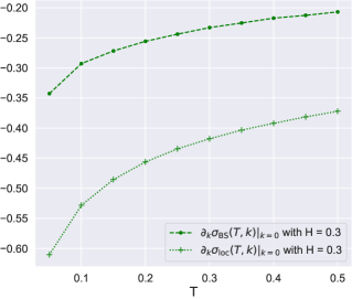
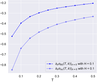
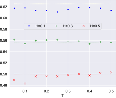
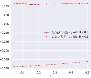
In our numerical experiments in section 4, we estimate the exact ATM local volatility skew 12kσloc(t,k)|k=0evaluated-at12subscript𝑘subscript𝜎loc𝑡𝑘𝑘0\frac{1}{2}\partial_{k}\sigma_{\mathrm{loc}}(t,k)\big{|}_{k=0} in the rough Bergomi model (4.1), and find perfect agreement with Corollary 3.4. The model local volatility skew can be observed in Figure 1, and the ratio of the implied volatility skew over the local volatility skew in Figure 2.

Remark 3.5.

When H=1/2𝐻12H=1/2, we are back to the classical 1/2121/2 skew rule, see Derman et al. [22].

Remark 3.6.

One can expect the 1H+3/21𝐻32\frac{1}{H+3/2} rule (3.13) to hold also for rough or rough-like volatility models that do not belong to the model class (2.1), such as the rough Heston model [27]. The recent preprint [19] provides numerical evidence for the 1H+3/21𝐻32\frac{1}{H+3/2} rule under the lifted Heston model [1], a Markovian approximation of rough Heston, as well as a formal proof in the case of the proper rough Heston model, see [19, Proposition 2.1]. In their recent work [2], Alos and co-authors prove the 1H+3/21𝐻32\frac{1}{H+3/2} rule for stochastic volatility models under suitable assumptions on the asymptotic behavior of the volatility process and related iterated Malliavin derivatives, further providing an asymptotic rule for the ratio of the at-the-money second derivative kk()|k=0evaluated-atsubscript𝑘𝑘𝑘0\partial_{kk}(\cdot)|_{k=0} of the local and implied volatility functions.

Remark 3.7 (The short-time harmonic mean formula and the 1/2 skew rule again).

When expressed in terms of an implied volatility σBSsubscript𝜎BS\sigma_{\mathrm{BS}}, Dupire’s formula for local volatility reads

σloc(t,k)2=σBS(t,k)+2ttσBS(t,k)(tkkσBS14t2σBS(kσBS)2+1σBS(1kkσBSσBS)2)(t,k)subscript𝜎locsuperscript𝑡𝑘2subscript𝜎BS𝑡𝑘2𝑡subscript𝑡subscript𝜎BS𝑡𝑘𝑡subscript𝑘𝑘subscript𝜎BS14superscript𝑡2subscript𝜎BSsuperscriptsubscript𝑘subscript𝜎BS21subscript𝜎BSsuperscript1𝑘subscript𝑘subscript𝜎BSsubscript𝜎BS2𝑡𝑘\sigma_{\mathrm{loc}}(t,k)^{2}=\frac{\sigma_{\mathrm{BS}}(t,k)+2\,t\,\partial_{t}\sigma_{\mathrm{BS}}(t,k)}{\Bigl{(}t\,\partial_{kk}\sigma_{\mathrm{BS}}-\frac{1}{4}t^{2}\,\sigma_{\mathrm{BS}}(\partial_{k}\sigma_{\mathrm{BS}})^{2}+\frac{1}{\sigma_{\mathrm{BS}}}\left(1-\frac{k\,\partial_{k}\sigma_{\mathrm{BS}}}{\sigma_{\mathrm{BS}}}\right)^{2}\Bigr{)}(t,k)} (3.14)

provided that σBSsubscript𝜎BS\sigma_{\mathrm{BS}} is sufficiently smooth for all the partial derivatives to make sense. Formally taking t0𝑡0t\to 0 inside (3.14) and assuming that the partial derivatives tσBSsubscript𝑡subscript𝜎BS\partial_{t}\sigma_{\mathrm{BS}}, kσBSsubscript𝑘subscript𝜎BS\partial_{k}\sigma_{\mathrm{BS}} and kkσBSsubscript𝑘𝑘subscript𝜎BS\partial_{kk}\sigma_{\mathrm{BS}} remain bounded, one obtains

σloc(0,k)2=σBS(0,k)2(1kσBS(0,k)σBS(0,k))2.subscript𝜎locsuperscript0𝑘2subscript𝜎BSsuperscript0𝑘2superscript1𝑘superscriptsubscript𝜎BS0𝑘subscript𝜎BS0𝑘2\sigma_{\mathrm{loc}}(0,k)^{2}=\frac{\sigma_{\mathrm{BS}}(0,k)^{2}}{\bigl{(}1-k\frac{\sigma_{\mathrm{BS}}^{\prime}(0,k)}{\sigma_{\mathrm{BS}}(0,k)}\bigr{)}^{2}}. (3.15)

The ordinary differential equation (3.15) can be used to reconstruct the function σBS(0,)subscript𝜎BS0\sigma_{\mathrm{BS}}(0,\cdot) from σloc(0,)subscript𝜎loc0\sigma_{\mathrm{loc}}(0,\cdot) and it is solved by the harmonic mean function

H(t,k)=11k0kdyσloc(t,y),𝐻𝑡𝑘11𝑘superscriptsubscript0𝑘d𝑦subscript𝜎loc𝑡𝑦H(t,k)=\frac{1}{\frac{1}{k}\int_{0}^{k}\frac{\mathrm{d}y}{\sigma_{\mathrm{loc}}(t,y)}}, (3.16)

evaluated at t=0𝑡0t=0. The computation above, leading from (3.15) to (3.16), can be found in [57]; the rigorous counterpart of this formal argument, that is the asymptotic equivalence σBS(t,k)H(t,k)similar-tosubscript𝜎BS𝑡𝑘𝐻𝑡𝑘\sigma_{\mathrm{BS}}(t,k)\sim H(t,k), known as the “harmonic mean formula” or BBF formula, was proven in [16] under the assumption that the local volatility surface σlocsubscript𝜎loc\sigma_{\mathrm{loc}} is bounded and uniformly continuous in a neighborhood of t=0𝑡0t=0. It is straightforward to see that the harmonic mean satisfies the property kH(t,k)|k=0=12kσloc(t,k)|k=0evaluated-atsubscript𝑘𝐻𝑡𝑘𝑘0evaluated-at12subscript𝑘subscript𝜎loc𝑡𝑘𝑘0\partial_{k}H(t,k)\big{|}_{k=0}=\frac{1}{2}\partial_{k}\sigma_{\mathrm{loc}}(t,k)\big{|}_{k=0}. Therefore, if we assume that the short-time approximation property σBS(t,k)H(t,k)subscript𝜎BS𝑡𝑘𝐻𝑡𝑘\sigma_{\mathrm{BS}}(t,k)\approx H(t,k) also holds for the first derivatives with respect to k𝑘k, as a consequence we obtain the 1/2121/2 short-time skew rule kσBS(t,0)12kσloc(t,0)similar-tosubscript𝑘subscript𝜎BS𝑡012subscript𝑘subscript𝜎loc𝑡0\partial_{k}\sigma_{\mathrm{BS}}(t,0)\sim\frac{1}{2}\partial_{k}\sigma_{\mathrm{loc}}(t,0) that we referred to in Remark 3.5.

Corollary 3.4 entails that the formal argument above does not hold anymore for the implied and local volatility surfaces generated by a rough stochastic volatility model. Notably, the boundedness of the partial derivatives tσBSsubscript𝑡subscript𝜎BS\partial_{t}\sigma_{\mathrm{BS}}, kσBSsubscript𝑘subscript𝜎BS\partial_{k}\sigma_{\mathrm{BS}} and kkσBSsubscript𝑘𝑘subscript𝜎BS\partial_{kk}\sigma_{\mathrm{BS}}, and the uniform continuity of the local volatility surface, fall short – but in such a way that the limit of the skew ratio 𝒮BS𝒮locsubscript𝒮BSsubscript𝒮loc\frac{\mathcal{S}_{\mathrm{BS}}}{\mathcal{S}_{\mathrm{loc}}} can still be identified and explicitly computed (see related numerical tests in Figure 4).

Remark 3.8 (Time-dependent volatility function).

The rough Bergomi model [6] comes with instantaneous variance

ξ(t)exp(ηxη22t2H)ξ(0)exp(ηx)=:σ2(x)\xi(t)\exp\Bigl{(}\eta x-\frac{\eta^{2}}{2}t^{2H}\Bigr{)}\sim\xi(0)\exp\bigl{(}\eta x\bigr{)}=:\sigma^{2}(x)

as t0𝑡0t\downarrow 0. We could have proved Theorem 3.3 and Corollary 3.4 in greater generality, with Vt=σ2(W^t,t)subscript𝑉𝑡superscript𝜎2subscript^𝑊𝑡𝑡V_{t}=\sigma^{2}(\widehat{W}_{t},t), provided the dependence with respect to t𝑡t in σ=σ(x,t)𝜎𝜎𝑥𝑡\sigma=\sigma(x,t) is sufficiently smooth such as not to affect the local analysis that underlies the proof. This is more subtle in the case of rough Bergomi where t2Hsuperscript𝑡2𝐻t^{2H} fails to be smooth at t=0+𝑡superscript0t=0^{+} when H<1/2𝐻12H<1/2. Even so, we discussed in [31] how to adjust the arguments to obtain exact asymptotics, the same logic applies here.

4 Numerical tests

We wish to estimate the conditional expectation (3.8) for some specific instance of the model (2.1), using Monte Carlo simulation. We consider the rough Bergomi model [6], for which the instantaneous variance process is given by

Vt=ξ0exp(ηW^tη22t2H)=ξ0exp(η0t2H(ts)H1/2dWsη22t2H),subscript𝑉𝑡subscript𝜉0𝜂subscript^𝑊𝑡superscript𝜂22superscript𝑡2𝐻subscript𝜉0𝜂superscriptsubscript0𝑡2𝐻superscript𝑡𝑠𝐻12differential-dsubscript𝑊𝑠superscript𝜂22superscript𝑡2𝐻V_{t}=\xi_{0}\exp\Bigl{(}\eta\widehat{W}_{t}-\frac{\eta^{2}}{2}t^{2H}\Bigr{)}=\xi_{0}\exp\Bigl{(}\eta\int_{0}^{t}\sqrt{2H}(t-s)^{H-1/2}\mathrm{d}W_{s}-\frac{\eta^{2}}{2}t^{2H}\Bigr{)}, (4.1)

where ξ0=V0subscript𝜉0subscript𝑉0\xi_{0}=V_{0} is the spot variance and η𝜂\eta a parameter that tunes the volatility of variance. Note that, strictly speaking, Theorem 3.3 and Corollary 3.4 do not apply to the model above, because of the time dependence in the volatility function σ(x,t)=ξ0exp(η2xη24t2H)𝜎𝑥𝑡subscript𝜉0𝜂2𝑥superscript𝜂24superscript𝑡2𝐻\sigma(x,t)=\sqrt{\xi_{0}}\exp\bigl{(}\frac{\eta}{2}x-\frac{\eta^{2}}{4}t^{2H}\bigr{)}. In light of the discussion in Remark 3.8, we can expect our asymptotic results to hold for such a time-dependent volatility function as well, which is in line with the output of our numerical experiments below.

For a given time horizon T>0𝑇0T>0 and a number N𝑁superscriptN\in\mathbb{N}^{*} of time-steps, the random vector (logVtk)1kNsubscriptsubscript𝑉subscript𝑡𝑘1𝑘𝑁(\log V_{t_{k}})_{1\leq k\leq N}, tk=kTNsubscript𝑡𝑘𝑘𝑇𝑁t_{k}=k\frac{T}{N}, has a multivariate Gaussian distribution with known mean and variance, see for example [6], and can therefore be simulated exactly. We use the standard simulation method for Gaussian vectors based on a Cholesky factorization of the covariance matrix. Of course, this method has a considerable complexity – cost 𝒪(N3)𝒪superscript𝑁3\mathcal{O}(N^{3}) for the Cholesky factorization and 𝒪(N2)𝒪superscript𝑁2\mathcal{O}(N^{2}) for the matrix multiplication required to get one sample of (Vtk)0kNsubscriptsubscript𝑉subscript𝑡𝑘0𝑘𝑁(V_{t_{k}})_{0\leq k\leq N} – but our focus is on the accuracy of our estimations, rather than on their computational time. We construct approximate samples of the log-asset price XT=120TVtdt+0TVt(ρdWt+ρ¯dW¯t)subscript𝑋𝑇12superscriptsubscript0𝑇subscript𝑉𝑡differential-d𝑡superscriptsubscript0𝑇subscript𝑉𝑡𝜌dsubscript𝑊𝑡¯𝜌dsubscript¯𝑊𝑡X_{T}=-\frac{1}{2}\int_{0}^{T}V_{t}\mathrm{d}t+\int_{0}^{T}\sqrt{V_{t}}(\rho\mathrm{d}W_{t}+\overline{\rho}\mathrm{d}\overline{W}_{t}) using a forward Euler scheme on the same time-grid

XTN=T2Nk=0N1Vtk+k=0N1Vtk(ρ(Wtk+1Wtk)+ρ¯(W¯tk+1W¯tk)).subscriptsuperscript𝑋𝑁𝑇𝑇2𝑁superscriptsubscript𝑘0𝑁1subscript𝑉subscript𝑡𝑘superscriptsubscript𝑘0𝑁1subscript𝑉subscript𝑡𝑘𝜌subscript𝑊subscript𝑡𝑘1subscript𝑊subscript𝑡𝑘¯𝜌subscript¯𝑊subscript𝑡𝑘1subscript¯𝑊subscript𝑡𝑘X^{N}_{T}=-\frac{T}{2N}\sum_{k=0}^{N-1}V_{t_{k}}+\sum_{k=0}^{N-1}\sqrt{V_{t_{k}}}\Bigl{(}\rho(W_{t_{k+1}}-W_{t_{k}})+\overline{\rho}(\overline{W}_{t_{k+1}}-\overline{W}_{t_{k}})\Bigr{)}.

Therefore, we obtain M𝑀M i.i.d. approximate Monte Carlo samples (XTN,m,VTm)1mMsubscriptsubscriptsuperscript𝑋𝑁𝑚𝑇subscriptsuperscript𝑉𝑚𝑇1𝑚𝑀(X^{N,m}_{T},V^{m}_{T})_{1\leq m\leq M} of the couple (XTN,VT)superscriptsubscript𝑋𝑇𝑁subscript𝑉𝑇(X_{T}^{N},V_{T}), from which our estimators of the implied volatility and local volatility (3.8) are constructed, as detailed below. Since our goal is to check the asymptotic statements appearing in Theorem 3.3 and Corollary 3.4, we will consider a large number N𝑁N of discretization steps and a large number M𝑀M of Monte Carlo samples in order to increase the precision of the estimates we use as a benchmark. We estimate out-of-the-money put and call option prices by standard empirical means and evaluate the corresponding implied volatilities σBS(T,K)subscript𝜎BS𝑇𝐾\sigma_{\mathrm{BS}}(T,K) by Newton’s search.

The rough Bergomi model (4.1) parameters we used in our experiments are S0=1,η=1.0,ρ=0.7formulae-sequencesubscript𝑆01formulae-sequence𝜂1.0𝜌0.7S_{0}=1,\eta=1.0,\rho=-0.7, and ξ0=0.2352subscript𝜉0superscript0.2352\xi_{0}=0.235^{2}. We tested three different values of H(0,1/2]𝐻012H\in(0,1/2], namely H{0.1,0.3,0.5}𝐻0.10.30.5H\in\{0.1,0.3,0.5\}. We used M=1.5×10⁶𝑀1.5superscript106M=1.5\times 10^{6} Monte Carlo samples and N=500𝑁500N=500 discretization points.

Remark 4.1.

Several recent works [10, 9, 42, 30] study the weak error rate of rough Bergomi type models. Without going into (bibliographical) details, the weak rate has now been identified as 111 for H𝐻H above 1616\frac{1}{6} and 3H+123𝐻123H+\frac{1}{2} for H𝐻H below 1616\frac{1}{6}. Importantly, as H0𝐻0H\downarrow 0, a weak rate of 1212\frac{1}{2} persists. The fairly large number of time steps we considered in our experiments (N=500𝑁500N=500) is arguably enough to obtain good benchmark values when H𝐻H is close to 1212\frac{1}{2}, but we should bear in mind that the bias in the Monte Carlo estimation is expected to become more and more important as H𝐻H approaches zero. In this case, larger number of time steps might be required to get a trustworthy level of accuracy; of course, the complexity of the exact Cholesky method we exploited in our simulation of the Riemann–Liouville process makes the simulations very demanding for very large values of N𝑁N.

4.1 Local and implied volatility estimators

In this section, we present in detail the estimators we have implemented for the target objects: the at-the-money implied volatility skew kσBS(t,k)|k=0evaluated-atsubscript𝑘subscript𝜎BS𝑡𝑘𝑘0\partial_{k}\sigma_{\mathrm{BS}}(t,k)|_{k=0}, the local volatility function (or Markovian projection) σloc(,)subscript𝜎loc\sigma_{\mathrm{loc}}(\cdot,\cdot) in (3.8), and the local volatility skew kσloc(t,k)|k=0evaluated-atsubscript𝑘subscript𝜎loc𝑡𝑘𝑘0\partial_{k}\sigma_{\mathrm{loc}}(t,k)|_{k=0}.

The estimator of the implied volatility skew.

A representation of the first derivative kσBS(t,k)subscript𝑘subscript𝜎BS𝑡𝑘\partial_{k}\sigma_{\mathrm{BS}}(t,k) can be obtained by differentiating the equation defining the implied volatility σBSsubscript𝜎BS\sigma_{\mathrm{BS}} with respect to the log-moneyness k𝑘k. More precisely, denoting CBS(k,v)subscript𝐶BS𝑘𝑣C_{\mathrm{BS}}(k,v) the Black–Scholes price of a call option with log-moneyness k𝑘k and total volatility parameter v=tσ𝑣𝑡𝜎v=\sqrt{t}\,\sigma, we have

𝔼[(S0eXtS0ek)+]=CBS(k,tσBS(t,k)),𝔼delimited-[]superscriptsubscript𝑆0superscript𝑒subscript𝑋𝑡subscript𝑆0superscript𝑒𝑘subscript𝐶BS𝑘𝑡subscript𝜎BS𝑡𝑘\mathbb{E}\bigl{[}(S_{0}e^{X_{t}}-S_{0}e^{k})^{+}\bigr{]}=C_{\mathrm{BS}}\bigl{(}k,\sqrt{t}\,\sigma_{\mathrm{BS}}(t,k)\bigr{)}, (4.2)

for all k𝑘k and t𝑡t. Taking the derivative at both sides of (4.2) with respect to k𝑘k and using the expressions of the first-order Black–Scholes greeks kCBS(k,v)subscript𝑘subscript𝐶BS𝑘𝑣\partial_{k}C_{\mathrm{BS}}(k,v) and vCBS(k,v)subscript𝑣subscript𝐶BS𝑘𝑣\partial_{v}C_{\mathrm{BS}}(k,v), we have

kσBS(t,k)subscript𝑘subscript𝜎BS𝑡𝑘\displaystyle\partial_{k}\sigma_{\mathrm{BS}}(t,k) =kCBS(k,v)S0ek(Xtk)tvCBS(k,v)|v=tσBS(t,k)absentevaluated-atsubscript𝑘subscript𝐶BS𝑘𝑣subscript𝑆0superscript𝑒𝑘subscript𝑋𝑡𝑘𝑡subscript𝑣subscript𝐶BS𝑘𝑣𝑣𝑡subscript𝜎BS𝑡𝑘\displaystyle=\frac{-\partial_{k}C_{\mathrm{BS}}(k,v)-S_{0}e^{k}\,\mathbb{P}\bigl{(}X_{t}\geq k\bigr{)}}{\sqrt{t}\,\partial_{v}C_{\mathrm{BS}}(k,v)}\bigg{|}_{v=\sqrt{t}\,\sigma_{\mathrm{BS}}(t,k)}\,
=N(d2(k,v))(Xtk)tϕ(d2(k,v))|v=tσBS(t,k),absentevaluated-at𝑁subscript𝑑2𝑘𝑣subscript𝑋𝑡𝑘𝑡italic-ϕsubscript𝑑2𝑘𝑣𝑣𝑡subscript𝜎BS𝑡𝑘\displaystyle=\frac{N\bigl{(}d_{2}(k,v)\bigr{)}-\mathbb{P}\bigl{(}X_{t}\geq k\bigr{)}}{\sqrt{t}\,\phi\bigl{(}d_{2}(k,v)\bigr{)}}\bigg{|}_{v=\sqrt{t}\,\sigma_{\mathrm{BS}}(t,k)}\,,

where d2(k,v)=kvv2subscript𝑑2𝑘𝑣𝑘𝑣𝑣2d_{2}(k,v)=-\frac{k}{v}-\frac{v}{2}, and ϕitalic-ϕ\phi (resp. N𝑁N) denotes the standard Gaussian density (resp. cumulative distribution). The representation above for the implied volatility skew allows us to avoid finite difference methods and only requires us to estimate σBS(t,k)subscript𝜎BS𝑡𝑘\sigma_{\mathrm{BS}}(t,k) and (Xtk)subscript𝑋𝑡𝑘\mathbb{P}(X_{t}\geq k), which we can do with the same Monte Carlo sample, in order to estimate kσBS(t,k)subscript𝑘subscript𝜎BS𝑡𝑘\partial_{k}\sigma_{\mathrm{BS}}(t,k) (and therefore, in particular, the at-the-money skew kσBS(t,0)subscript𝑘subscript𝜎BS𝑡0\partial_{k}\sigma_{\mathrm{BS}}(t,0)).

The estimator of the local volatility function.

Given the Monte Carlo samples (XTN,m,VTm)1mMsubscriptsubscriptsuperscript𝑋𝑁𝑚𝑇subscriptsuperscript𝑉𝑚𝑇1𝑚𝑀(X^{N,m}_{T},V^{m}_{T})_{1\leq m\leq M} of the couple (XTN,VT)superscriptsubscript𝑋𝑇𝑁subscript𝑉𝑇(X_{T}^{N},V_{T}), the conditional expectation (3.8) defining the local volatility function can be estimated appealing to several different regression methods, see, e.g., [63, 53]. We have implemented and benchmarked two different estimators: on the one side, a kernel regressor, already applied to evaluate the Markovian projection within the celebrated particular calibration algorithm [50], and on the other side, an alternative estimator based on the explicit knowledge of the conditional law of (Xt,Vt)|(Ws)stconditionalsubscript𝑋𝑡subscript𝑉𝑡subscriptsubscript𝑊𝑠𝑠𝑡(X_{t},V_{t})|(W_{s})_{s\leq t}.

Our kernel regressor is the Nadaraya–Watson estimator with bandwidth δ𝛿\delta,

σloc2(t,k)=𝔼[Vt|Xt=k]m=1MVtmKδ(XtN,mk)m=1MKδ(XtN,mk).superscriptsubscript𝜎loc2𝑡𝑘𝔼delimited-[]conditionalsubscript𝑉𝑡subscript𝑋𝑡𝑘superscriptsubscript𝑚1𝑀superscriptsubscript𝑉𝑡𝑚subscript𝐾𝛿superscriptsubscript𝑋𝑡𝑁𝑚𝑘superscriptsubscript𝑚1𝑀subscript𝐾𝛿superscriptsubscript𝑋𝑡𝑁𝑚𝑘\sigma_{\mathrm{loc}}^{2}(t,k)=\mathbb{E}\left[V_{t}|X_{t}=k\right]\approx\frac{\sum_{m=1}^{M}V_{t}^{m}K_{\delta}\bigl{(}X_{t}^{N,m}-k\bigr{)}}{\sum_{m=1}^{M}K_{\delta}\bigl{(}X_{t}^{N,m}-k\bigr{)}}. (4.3)

We used a Gaussian kernel Kδ(x)=exp(δx2)subscript𝐾𝛿𝑥𝛿superscript𝑥2K_{\delta}(x)=\exp(-\delta x^{2}) in our tests.

On the other hand, it is a standard fact that conditionally on t=σ(Wu:ut)\mathcal{F}_{t}=\sigma(W_{u}:u\leq t), the instantaneous variance Vtsubscript𝑉𝑡V_{t} is known, while the log-price Xtsubscript𝑋𝑡X_{t} is normally distributed with mean 120tVsds+ρ0tVsdWs12superscriptsubscript0𝑡subscript𝑉𝑠differential-d𝑠𝜌superscriptsubscript0𝑡subscript𝑉𝑠differential-dsubscript𝑊𝑠-\frac{1}{2}\int_{0}^{t}V_{s}\mathrm{d}s+\rho\int_{0}^{t}\sqrt{V_{s}}\mathrm{d}W_{s} and variance (1ρ2)0tVsds1superscript𝜌2superscriptsubscript0𝑡subscript𝑉𝑠differential-d𝑠(1-\rho^{2})\int_{0}^{t}V_{s}\mathrm{d}s. This property yields a representation of the Markovian projection σloc(,)subscript𝜎loc\sigma_{\mathrm{loc}}(\cdot,\cdot) as the ratio of two expectations,

σloc2(t,k)=𝔼[Vt|Xt=k]=𝔼[VtΠt(k)]𝔼[Πt(k)]superscriptsubscript𝜎loc2𝑡𝑘𝔼delimited-[]conditionalsubscript𝑉𝑡subscript𝑋𝑡𝑘𝔼delimited-[]subscript𝑉𝑡subscriptΠ𝑡𝑘𝔼delimited-[]subscriptΠ𝑡𝑘\sigma_{\mathrm{loc}}^{2}(t,k)=\mathbb{E}\left[V_{t}|X_{t}=k\right]=\frac{\mathbb{E}\left[V_{t}\,\Pi_{t}(k)\right]}{\mathbb{E}\left[\Pi_{t}(k)\right]} (4.4)

where

Πt(k)=10tVsdsexp(12(1ρ2)0tVsds(k+120tVsdsρ0tVsdWs)2).subscriptΠ𝑡𝑘1superscriptsubscript0𝑡subscript𝑉𝑠differential-d𝑠121superscript𝜌2superscriptsubscript0𝑡subscript𝑉𝑠differential-d𝑠superscript𝑘12superscriptsubscript0𝑡subscript𝑉𝑠differential-d𝑠𝜌superscriptsubscript0𝑡subscript𝑉𝑠differential-dsubscript𝑊𝑠2\Pi_{t}(k)=\frac{1}{\sqrt{\int_{0}^{t}V_{s}\mathrm{d}s}}\exp\biggl{(}-\frac{1}{2(1-\rho^{2})\int_{0}^{t}V_{s}\mathrm{d}s}\Bigl{(}k+\frac{1}{2}\int_{0}^{t}V_{s}\mathrm{d}s-\rho\int_{0}^{t}\sqrt{V_{s}}\mathrm{d}W_{s}\Bigr{)}^{2}\biggr{)}.

A derivation of (4.4) can be found in [56, Proposition 3.1]; incidentally, this representation of σlocsubscript𝜎loc\sigma_{\mathrm{loc}} has been exploited in [52] in the context of a calibration strategy of local stochastic volatility models – prior to the particular algorithm [50].

The estimator of the local volatility skew.

Differentiating the right-hand side of (4.4) with respect to k𝑘k, we obtain a representation of kσloc(t,k)subscript𝑘subscript𝜎loc𝑡𝑘\partial_{k}\sigma_{\mathrm{loc}}(t,k):

kσloc(t,k)=k(𝔼[VtΠt]𝔼[Πt])2σloc(t,k)=𝔼[VtΠt]𝔼[U0tVsdsΠt]𝔼[U0tVsdsΠtVt]𝔼[Πt]2(1ρ2)𝔼[VtΠt]1/2𝔼[Πt]3/2,subscript𝑘subscript𝜎loc𝑡𝑘𝑘𝔼delimited-[]subscript𝑉𝑡subscriptΠ𝑡𝔼delimited-[]subscriptΠ𝑡2subscript𝜎loc𝑡𝑘𝔼delimited-[]subscript𝑉𝑡subscriptΠ𝑡𝔼delimited-[]𝑈superscriptsubscript0𝑡subscript𝑉𝑠differential-d𝑠subscriptΠ𝑡𝔼delimited-[]𝑈superscriptsubscript0𝑡subscript𝑉𝑠differential-d𝑠subscriptΠ𝑡subscript𝑉𝑡𝔼delimited-[]subscriptΠ𝑡21superscript𝜌2𝔼superscriptdelimited-[]subscript𝑉𝑡subscriptΠ𝑡12𝔼superscriptdelimited-[]subscriptΠ𝑡32\partial_{k}\sigma_{\mathrm{loc}}(t,k)=\frac{\frac{\partial}{\partial k}\left(\frac{\mathbb{E}\left[V_{t}\Pi_{t}\right]}{\mathbb{E}\left[\Pi_{t}\right]}\right)}{2\,\sigma_{\mathrm{loc}}(t,k)}=\frac{\mathbb{E}\left[V_{t}\Pi_{t}\right]\mathbb{E}\left[\frac{U}{\int_{0}^{t}V_{s}\mathrm{d}s}\Pi_{t}\right]-\mathbb{E}\left[\frac{U}{\int_{0}^{t}V_{s}\mathrm{d}s}\Pi_{t}V_{t}\right]\mathbb{E}\left[\Pi_{t}\right]}{2(1-\rho^{2})\mathbb{E}\left[V_{t}\Pi_{t}\right]^{1/2}\mathbb{E}\left[\Pi_{t}\right]^{3/2}}\,, (4.5)

where ΠtsubscriptΠ𝑡\Pi_{t} is a shorthand for Πt(k)subscriptΠ𝑡𝑘\Pi_{t}(k), U=U(k)=k+120tVsdsρ0tVsdWs𝑈𝑈𝑘𝑘12superscriptsubscript0𝑡subscript𝑉𝑠differential-d𝑠𝜌superscriptsubscript0𝑡subscript𝑉𝑠differential-dsubscript𝑊𝑠U=U(k)=k+\frac{1}{2}\int_{0}^{t}V_{s}\mathrm{d}s-\rho\int_{0}^{t}\sqrt{V_{s}}\mathrm{d}W_{s}, and Πtk=U(1ρ2)0tVsdsΠtsubscriptΠ𝑡𝑘𝑈1superscript𝜌2superscriptsubscript0𝑡subscript𝑉𝑠differential-d𝑠subscriptΠ𝑡\frac{\partial\Pi_{t}}{\partial k}=-\frac{U}{(1-\rho^{2})\int_{0}^{t}V_{s}\mathrm{d}s}\,\Pi_{t}. All the expectations appearing in (4.4) and (4.5) can be estimated based on the exact simulation of the discretized variance path (Vtk)1kNsubscriptsubscript𝑉subscript𝑡𝑘1𝑘𝑁(V_{t_{k}})_{1\leq k\leq N}; we approximate the integrals 0tVsdssuperscriptsubscript0𝑡subscript𝑉𝑠differential-d𝑠\int_{0}^{t}V_{s}\mathrm{d}s and 0tVsdWssuperscriptsubscript0𝑡subscript𝑉𝑠differential-dsubscript𝑊𝑠\int_{0}^{t}\sqrt{V_{s}}\mathrm{d}W_{s} using left-point Euler schemes. Note that the resulting non-parametric estimators based on the representations (4.4) and (4.5) do not contain any kernel bandwidth or other hyper-parameters to be tuned. This is a clear advantage with respect to (4.3). We have nevertheless tested both estimators (4.3) and (4.4) for the Markovian projection function, and found perfect agreement between the two in our tests – in other words, the local volatilities and local volatility skews computed with the two different methods would be indistinguishable in Figures 1 and 3.

In Figure 1, we plot the term structure of the ATM implied and local volatility skews, for three different values of H𝐻H and maturities up to T=0.5𝑇0.5T=0.5 years. As pointed out in the Introduction and in section 2, the power-law behavior of the ATM implied volatility skew generated by the rough Bergomi model is already well-known; on the other hand, the power-law behavior observed for the local volatility skew in Figure 1 is (to the best of our knowledge) new, and consistent with Corollary 3.4. Figure 2 shows the ratio of the implied volatility ATM skew over the local volatility ATM skew, that is the ratio of the curves observed in Figure 1, for the different values of H𝐻H: the numerical results are in very good agreement with the “1H+3/21𝐻32\frac{1}{H+3/2} rule” announced in Corollary 3.4. Additionally, we note that the ratio of the two skews seems to be rather stable – its value is almost constant for maturities up to T=0.5𝑇0.5T=0.5 years, with our parameter setup.

4.2 Short-dated local volatility

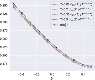
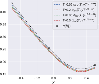
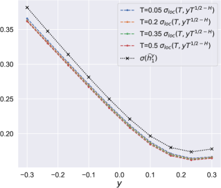
Theorem 3.3 gives the asymptotic behavior of σloc(T,yT1/2H)subscript𝜎loc𝑇𝑦superscript𝑇12𝐻\sigma_{\mathrm{loc}}\bigl{(}T,y\,T^{1/2-H}\bigr{)} as T𝑇T becomes small. Since y𝑦y is allowed to vary around the at-the-money point y=0𝑦0y=0, we can check whether the limit (3.9) holds for the function yσ^loc(T,y):=σloc(T,yT1/2H)maps-to𝑦subscript^𝜎loc𝑇𝑦assignsubscript𝜎loc𝑇𝑦superscript𝑇12𝐻y\mapsto\widehat{\sigma}_{\mathrm{loc}}(T,y):=\sigma_{\mathrm{loc}}\bigl{(}T,y\,T^{1/2-H}\bigr{)}, that is the whole local volatility smile rescaled with maturity. The computation of the limiting function σ(h^1y)𝜎subscriptsuperscript^𝑦1\sigma\bigl{(}\widehat{h}^{y}_{1}\bigr{)} requires us to evaluate the Cameron-Martin path hyH1superscript𝑦superscript𝐻1h^{y}\in H^{1} that minimizes the rate function in (3.2), for given y𝑦y. We follow the procedure already exploited in [28] and [32, section 5.1] : it can be shown, see [28], that the rate function satisfies the alternative representation Λ(y)=inf{(yρG(h))22ρ¯2F(h)+12h˙,h˙:h˙L2(0,1)}Λ𝑦infimumconditional-setsuperscript𝑦𝜌𝐺22superscript¯𝜌2𝐹12˙˙˙superscript𝐿201\Lambda(y)=\inf\Bigl{\{}\frac{(y-\rho\,G(h))^{2}}{2\,\overline{\rho}^{2}F(h)}+\frac{1}{2}\langle\dot{h},\dot{h}\rangle:\dot{h}\in L^{2}(0,1)\Bigr{\}}, with F(h)=σ2(h^),1=01σ2(h^t)dt𝐹superscript𝜎2^1superscriptsubscript01superscript𝜎2subscript^𝑡differential-d𝑡F(h)=\langle\sigma^{2}(\widehat{h}),1\rangle=\int_{0}^{1}\sigma^{2}(\widehat{h}_{t})\mathrm{d}t and G(h)=σ(h^),h˙=01σ(h^t)h˙tdt𝐺𝜎^˙superscriptsubscript01𝜎subscript^𝑡subscript˙𝑡differential-d𝑡G(h)=\langle\sigma(\widehat{h}),\dot{h}\rangle=\int_{0}^{1}\sigma(\widehat{h}_{t})\dot{h}_{t}\mathrm{d}t. This alternative representation yields the rate function under the form of an unconstrained optimization problem (as opposed to the constrained optimization in (3.2)), which can then be approximately solved by the projection of the one-dimensional path hh over an orthonormal basis {e˙n}n1subscriptsubscript˙𝑒𝑛𝑛1\{\dot{e}_{n}\}_{n\geq 1} of L2superscript𝐿2L^{2}, h˙t=n1ane˙n(t)subscript˙𝑡subscript𝑛1subscript𝑎𝑛subscript˙𝑒𝑛𝑡\dot{h}_{t}=\sum_{n\geq 1}a_{n}\dot{e}_{n}(t). In practice, we truncate the sum at a certain order N𝑁N and minimize over the coefficients (an)1nNsubscriptsubscript𝑎𝑛1𝑛𝑁(a_{n})_{1\leq n\leq N}; we obtain an approximation of the minimizer hysuperscript𝑦h^{y} and therefore of h^ty=(KHh˙y)t=0tK(t,s)h˙sdssubscriptsuperscript^𝑦𝑡subscriptsuperscript𝐾𝐻superscript˙𝑦𝑡superscriptsubscript0𝑡𝐾𝑡𝑠subscript˙𝑠differential-d𝑠\widehat{h}^{y}_{t}=(K^{H}*\dot{h}^{y})_{t}=\int_{0}^{t}K(t,s)\dot{h}_{s}\mathrm{d}s. We chose the Fourier basis {e˙1(t)=1,e˙2n(t)=2cos(2πnt),e˙2n+1(t)=2sin(2πnt),n{0}}formulae-sequencesubscript˙𝑒1𝑡1formulae-sequencesubscript˙𝑒2𝑛𝑡22𝜋𝑛𝑡formulae-sequencesubscript˙𝑒2𝑛1𝑡22𝜋𝑛𝑡𝑛0\bigl{\{}\dot{e}_{1}(t)=1,\ \dot{e}_{2n}(t)=\sqrt{2}\cos(2\pi n\,t),\ \dot{e}_{2n+1}(t)=\sqrt{2}\sin(2\pi n\,t),n\in\mathbb{N}\setminus\{0\}\bigr{\}} in our experiments, and observed that truncation of the sum at N=8𝑁8N=8 provides a good accuracy. The results for the rough Bergomi model are displayed in Figure 3, where the function σ^loc(T,y)subscript^𝜎loc𝑇𝑦\widehat{\sigma}_{\mathrm{loc}}(T,y) is indeed seen to approach its limit σ(h^1y)𝜎subscriptsuperscript^𝑦1\sigma\bigl{(}\widehat{h}^{y}_{1}\bigr{)} when maturity decreases from T=0.5𝑇0.5T=0.5 to T=0.05𝑇0.05T=0.05. The residual error term σ^loc(T,y)σ(h^1y)subscript^𝜎loc𝑇𝑦𝜎subscriptsuperscript^𝑦1\widehat{\sigma}_{\mathrm{loc}}(T,y)-\sigma\bigl{(}\widehat{h}^{y}_{1}\bigr{)} is seen to depend on H𝐻H, with lower values of H𝐻H being associated with higher errors. It is however unclear whether the error for H=0.1𝐻0.1H=0.1 is due to the slow convergence of σ^locsubscript^𝜎loc\widehat{\sigma}_{\mathrm{loc}} or the weak error rate due to the Monte Carlo simulation (see Remark 4.1).

Extrapolation of local volatility surfaces.

Eventually, Theorem 3.3 provides us with an extrapolation recipe of local volatilities for very short maturities: fixing a (small) maturity T𝑇T and a log-moneyness level k𝑘k, formally plugging y=kT1/2H𝑦𝑘superscript𝑇12𝐻y=\frac{k}{T^{1/2-H}} in (3.9) we obtain

σloc(T,k)σ(h^1y)|y=kT1/2H.subscript𝜎loc𝑇𝑘evaluated-at𝜎superscriptsubscript^1𝑦𝑦𝑘superscript𝑇12𝐻\sigma_{\mathrm{loc}}\bigl{(}T,k\bigr{)}\approx\sigma\Bigl{(}\widehat{h}_{1}^{y}\Bigr{)}\Bigr{|}_{y=\frac{k}{T^{1/2-H}}}\,.

The limiting function σ(h^1y)|y=kT1/2Hevaluated-at𝜎superscriptsubscript^1𝑦𝑦𝑘superscript𝑇12𝐻\sigma\bigl{(}\widehat{h}_{1}^{y}\bigr{)}|_{y=\frac{k}{T^{1/2-H}}} can therefore be used to extrapolate a local volatility surface in a way that is consistent with the behavior implied by a rough volatility model.

As a specific application, consider the calibration of a local-stochastic volatility model (LSV) to an option price surface, for example using the particle method of Guyon and Henry-Labordère [50]. The LSV model can be obtained by the decoration of a naked rough volatility model, which amounts to enhancing the rough volatility model (2.1) for St=S0eXtsubscript𝑆𝑡subscript𝑆0superscript𝑒subscript𝑋𝑡S_{t}=S_{0}e^{X_{t}} with a leverage function l(t,S)𝑙𝑡𝑆l(t,S),

dSt=Stl(t,St)Vt(ρdWt+1ρ2dW¯t).dsubscript𝑆𝑡subscript𝑆𝑡𝑙𝑡subscript𝑆𝑡subscript𝑉𝑡𝜌dsubscript𝑊𝑡1superscript𝜌2dsubscript¯𝑊𝑡\mathrm{d}S_{t}=S_{t}\,l(t,S_{t})\sqrt{V_{t}}\left(\rho\,\mathrm{d}W_{t}+\sqrt{1-\rho^{2}}\,\mathrm{d}\overline{W}_{t}\right)\,.

Given the spot variance process V𝑉V, the LSV model calibrated to a given Dupire local volatility surface σDupsubscript𝜎Dup\sigma_{\mathrm{Dup}}, corresponds to (see [50])

l(t,St)=σDup(t,St)𝔼[Vt|St].𝑙𝑡subscript𝑆𝑡subscript𝜎Dup𝑡subscript𝑆𝑡𝔼delimited-[]conditionalsubscript𝑉𝑡subscript𝑆𝑡l(t,S_{t})=\frac{\sigma_{\mathrm{Dup}}(t,S_{t})}{\sqrt{\mathbb{E}[V_{t}|S_{t}]}}.

In general, one wishes the leverage function l(t,S)𝑙𝑡𝑆l(t,S) to be a small correction to the original stochastic volatility model (in other words: as close as possible to l1𝑙1l\equiv 1). In practice, the local volatility σDupsubscript𝜎Dup\sigma_{\mathrm{Dup}} coming from market data has to be extrapolated for values of t𝑡t smaller than the shorter observed maturity, and the choice of the extrapolation method is up to the user. If, for small t𝑡t, the chosen extrapolation σDup(t,K)subscript𝜎Dup𝑡𝐾\sigma_{\mathrm{Dup}}(t,K) is qualitatively too different from the behavior of the conditional expectation 𝔼[Vt|St=K]𝔼delimited-[]conditionalsubscript𝑉𝑡subscript𝑆𝑡𝐾\mathbb{E}[V_{t}|S_{t}=K] in the rough volatility setting (for example, more specifically: the ATM skew of σDupsubscript𝜎Dup\sigma_{\mathrm{Dup}} is far from the power law (3.12)), then the leverage function will have to compensate, hence deviating from the unit function. Under the pure rough volatility model (l1𝑙1l\equiv 1), Theorem 3.3 and Corollary 3.4 describe the behavior of the Markovian projection 𝔼[Vt|St]𝔼delimited-[]conditionalsubscript𝑉𝑡subscript𝑆𝑡\mathbb{E}[V_{t}|S_{t}] for small t𝑡t: eventually, these statements give hints on how σDup(t,)subscript𝜎Dup𝑡\sigma_{\mathrm{Dup}}(t,\cdot) should be extrapolated for l(t,)𝑙𝑡l(t,\cdot) not to deviate too much from the unit function. Such an extrapolation scheme is exploited in the recent work of Dall’Acqua, Longoni and Pallavicini [19], precisely in order to calibrate a LSV model with lifted Heston [1] backbone to the implied volatility surface of the EuroStoxx50 index.111We thank Andrea Pallavicini and Riccardo Longoni for interesting and stimulating discussions on this topic.

Failure of the harmonic mean asymptotic formula under rough volatility.

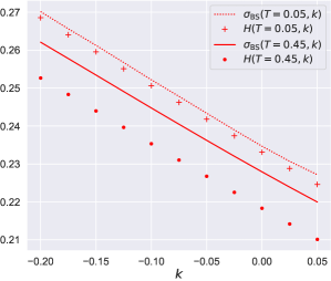
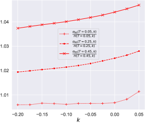
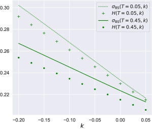
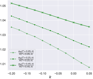
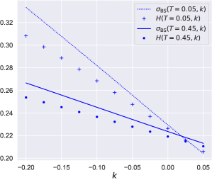
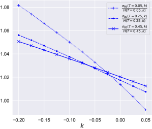
In Remark 3.7, we pointed out that, as a consequence of the general 1H+3/21𝐻32\frac{1}{H+3/2} skew rule (as opposed to the 1/2121/2 rule) in Corollary 3.4, the harmonic mean asymptotic formula σBS(T,k)H(T,k)similar-tosubscript𝜎BS𝑇𝑘𝐻𝑇𝑘\sigma_{\mathrm{BS}}(T,k)\sim H(T,k) as T0𝑇0T\to 0, see (3.16), is expected not to hold for H1/2𝐻12H\neq 1/2 (without any contradiction with the statements in [16], which require regularity conditions on local volatility surface that are not satisfied in the rough volatility setting, see our discussion in Remark 3.7). In other words, we do not expect the harmonic mean of the local volatility H(T,k)=11k0kdyσloc(T,y)𝐻𝑇𝑘11𝑘superscriptsubscript0𝑘d𝑦subscript𝜎loc𝑇𝑦H(T,k)=\frac{1}{\frac{1}{k}\int_{0}^{k}\frac{\mathrm{d}y}{\sigma_{\mathrm{loc}}(T,y)}} to be a good approximation of the implied volatility when maturities become small when the involved volatility surfaces are generated by a rough vol model. Having constructed estimators (4.3) and (4.4) of the local volatility function under the rough Bergomi model, we are also able to approximate (with an additional deterministic quadrature) the harmonic mean H(T,k)𝐻𝑇𝑘H(T,k), and compare the output with the implied volatility smile. The results are shown in Figure 4, for three different values of H𝐻H. As expected, when H=0.5𝐻0.5H=0.5 we observe (upper left panel) that the implied volatility σBS(T,k)subscript𝜎BS𝑇𝑘\sigma_{\mathrm{BS}}(T,k) approaches the harmonic mean H(T,k)𝐻𝑇𝑘H(T,k) when maturity decreases from T=0.45𝑇0.45T=0.45 to T=0.05𝑇0.05T=0.05, and the at-the-money slopes are also seen to agree. The convergence is even more apparent in the upper right figure, where the ratio σBS(T,k)H(T,k)subscript𝜎BS𝑇𝑘𝐻𝑇𝑘\frac{\sigma_{\mathrm{BS}}(T,k)}{H(T,k)} is seen to monotonically converge to one. This behavior should be compared with the one in the two bottom figures, where the rough case H=0.1𝐻0.1H=0.1 is considered (the case H=0.3𝐻0.3H=0.3 being intermediate between the other two): now, when maturity decreases, the implied volatility smile does not seem to approach the harmonic mean H(T,k)𝐻𝑇𝑘H(T,k) anymore (apart from the specific at-the-money point k=0𝑘0k=0 where both functions tend to the initial spot volatility σ0=V0subscript𝜎0subscript𝑉0\sigma_{0}=\sqrt{V_{0}}), and in particular, the slopes of the two curves are seen to considerably deviate from each other. This phenomenon is even more clear in the bottom right figure, where the ratio σBS(T,k)H(T,k)subscript𝜎BS𝑇𝑘𝐻𝑇𝑘\frac{\sigma_{\mathrm{BS}}(T,k)}{H(T,k)} has a completely different behavior with respect to the diffusive case H=0.5𝐻0.5H=0.5.

References

  • [1] E. Abi Jaber. Lifting the heston model. Quantitative Finance, 19(12):1995–2013, 2019.
  • [2] E. Alòs, D. García-Lorite, and M. Pravosud. On the skew and curvature of implied and local volatilities. arXiv e-prints, https://arxiv.org/pdf/2205.11185.pdf, 2022.
  • [3] E. Alòs, J. A. León, and J. Vives. On the short-time behavior of the implied volatility for jump-diffusion models with stochastic volatility. Finance and Stochastics, 11(4):571–589, 2007.
  • [4] R. Azencott. Petites perturbations aléatoires des systèmes dynamiques: développements asymptotiques. Bulletin des sciences mathématiques, 109(3):253–308, 1985.
  • [5] V. Bally. An elementary introduction to Malliavin calculus. Research Report RR-4718, INRIA. Available at https://hal.inria.fr/inria-00071868., 2003.
  • [6] C. Bayer, P. Friz, and J. Gatheral. Pricing under rough volatility. Quantitative Finance, 16(6):887–904, 2016.
  • [7] C. Bayer, P. K. Friz, P. Gassiat, J. Martin, and B. Stemper. A regularity structure for rough volatility. Mathematical Finance, 30(3):782–832, 2020.
  • [8] C. Bayer, P. K. Friz, A. Gulisashvili, B. Horvath, and B. Stemper. Short-time near-the-money skew in rough fractional volatility models. Quantitative Finance, 19(5):779–798, 2019.
  • [9] C. Bayer, M. Fukasawa, and S. Nakahara. Short communication: On the weak convergence rate in the discretization of rough volatility models. SIAM Journal on Financial Mathematics, 13(3), 2022.
  • [10] C. Bayer, E. J. Hall, and R. Tempone. Weak error rates for option pricing under the rough bergomi model. arXiv preprint arXiv:2009.01219, and to appear in IJTAF, 2020.
  • [11] C. Bayer, C. B. Hammouda, and R. Tempone. Hierarchical adaptive sparse grids and quasi-Monte Carlo for option pricing under the rough Bergomi model. Quantitative Finance, 0(0):1–17, 2020.
  • [12] C. Bayer, F. A. Harang, and P. Pigato. Log-Modulated Rough Stochastic Volatility Models. SIAM Journal on Financial Mathematics, 12(3):1257–1284, 2021.
  • [13] C. Bayer, B. Horvath, A. Muguruza, B. Stemper, and M. Tomas. On deep calibration of (rough) stochastic volatility models. arXiv preprint arXiv:1908.08806, 2019.
  • [14] M. Bennedsen, A. Lunde, and M. S. Pakkanen. Hybrid scheme for Brownian semistationary processes. Finance and Stochastics, 21(4):931–965, 2017.
  • [15] M. Bennedsen, A. Lunde, and M. S. Pakkanen. Decoupling the Short- and Long-Term Behavior of Stochastic Volatility. Journal of Financial Econometrics, 2021.
  • [16] H. Berestycki, J. Busca, and I. Florent. Asymptotics and calibration of local volatility models. Quantitative Finance, 2:61–69, 2002.
  • [17] H. Berestycki, J. Busca, and I. Florent. Computing the implied volatility in stochastic volatility models. Communications on Pure and Applied Mathematics, 57(10):1352–1373, 2004.
  • [18] G. Brunick and S. Shreve. Mimicking an Itô process by a solution of a stochastic differential equation. The Annals of Applied Probability, 23(4):1584 – 1628, 2013.
  • [19] E. Dall’Acqua, R. Longoni, and A. Pallavicini. Rough-heston local-volatility model. arXiv e-prints, https://arxiv.org/abs/2206.09220, 2022.
  • [20] S. De Marco, P. Friz, and S. Gerhold. Rational shapes of local volatility. Risk, 26(2):70, 2013.
  • [21] S. De Marco and P. K. Friz. Local Volatility, Conditioned Diffusions, and Varadhan’s Formula. SIAM Journal on Financial Mathematics, 9(2):835–874, 2018.
  • [22] E. Derman, I. Kani, and J. Z. Zou. The local volatility surface: Unlocking the information in index option prices. Financial Analysts Journal, 52(4):25–36, 1996.
  • [23] B. Dupire. Pricing with a smile. Risk, 7(1):18–20, 1994.
  • [24] B. Dupire. A unified theory of volatility. Derivatives pricing: The classic collection, 2004 (P. Carr, ed.), pages 185–196, 1996.
  • [25] O. El Euch, M. Fukasawa, J. Gatheral, and M. Rosenbaum. Short-term at-the-money asymptotics under stochastic volatility models. SIAM Journal on Financial Mathematics, 10(2):491–511, 2019.
  • [26] O. El Euch, M. Fukasawa, and M. Rosenbaum. The microstructural foundations of leverage effect and rough volatility. Finance and Stochastics, 22(2):241–280, 2018.
  • [27] O. El Euch and M. Rosenbaum. The characteristic function of rough Heston models. Mathematical Finance, 29(1):3–38, 2019.
  • [28] M. Forde and H. Zhang. Asymptotics for rough stochastic volatility models. SIAM Journal on Financial Mathematics, 8(1):114–145, 2017.
  • [29] E. Fournié, J.-M. Lasry, J. Lebuchoux, and P.-L. Lions. Applications of Malliavin calculus to Monte-Carlo methods in finance. II. Finance and Stochastics, 5(2):201–236, 2001.
  • [30] P. Friz, W. Salkeld, and T. Wagenhofer. Weak error estimates for rough volatility models. arXiv, 2022.
  • [31] P. K. Friz, P. Gassiat, and P. Pigato. Precise asymptotics: Robust stochastic volatility models. The Annals of Applied Probability, 31(2):896–940, 2021.
  • [32] P. K. Friz, P. Gassiat, and P. Pigato. Short-dated smile under rough volatility: asymptotics and numerics. Quantitative Finance, pages 1–18, 2021.
  • [33] P. K. Friz, J. Gatheral, A. Gulisashvili, A. Jacquier, and J. Teichmann. Large deviations and asymptotic methods in finance, volume 110. Springer, 2015.
  • [34] P. K. Friz, S. Gerhold, and M. Yor. How to make Dupire’s local volatility work with jumps. Quantitative Finance, 14(8):1327–1331, 2014.
  • [35] P. K. Friz and M. Hairer. A Course on Rough Paths. With an introduction to regularity structures. Springer, 2020.
  • [36] P. K. Friz, P. Pigato, and J. Seibel. The Step Stochastic Volatility Model. Risk, June, 2021.
  • [37] M. Fukasawa. Asymptotic analysis for stochastic volatility: martingale expansion. Finance and Stochastics, 15(4):635–654, 2011.
  • [38] M. Fukasawa. Short-time at-the-money skew and rough fractional volatility. Quantitative Finance, 17(2):189–198, 2017.
  • [39] M. Fukasawa. Volatility has to be rough. Quantitative Finance, 21(1):1–8, 2021.
  • [40] M. Fukasawa, T. Takabatake, and R. Westphal. Is Volatility Rough? arXiv preprint arXiv:1905.04852, 2019.
  • [41] P. Gassiat. On the martingale property in the rough Bergomi model. Electron. Commun. Probab., 24:9 pp., 2019.
  • [42] P. Gassiat. Weak error rates of numerical schemes for rough volatility. arXiv preprint arXiv:2203.09298, 2022.
  • [43] J. Gatheral. The volatility surface: a practitioner’s guide. John Wiley & Sons, 2006.
  • [44] J. Gatheral, E. P. Hsu, P. Laurence, C. Ouyang, and T.-H. Wang. Asymptotics of implied volatility in local volatility models. Mathematical Finance, 22(4):591–620, 2012.
  • [45] J. Gatheral, T. Jaisson, and M. Rosenbaum. Volatility is rough. Quantitative Finance, pages 1–17, 2018.
  • [46] J. Gatheral and M. Keller-Ressel. Affine forward variance models. Finance and Stochastics, 23(3):501–533, 2019.
  • [47] L. Goudenège, A. Molent, and A. Zanette. Machine learning for pricing American options in high-dimensional Markovian and non-Markovian models. Quantitative Finance, 20(4):573–591, 2020.
  • [48] A. Gulisashvili. Large deviation principle for volterra type fractional stochastic volatility models. SIAM Journal on Financial Mathematics, 9(3):1102–1136, 2018.
  • [49] A. Gulisashvili. Gaussian stochastic volatility models: Scaling regimes, large deviations, and moment explosions. Stochastic Processes and their Applications, 130(6):3648 – 3686, 2020.
  • [50] J. Guyon and P. Henry-Labordère. Being particular about calibration. Risk, January, 2012.
  • [51] I. Gyongy. Mimicking the one-dimensional marginal distributions of processes having an Itô differential. Probab. Th. Rel. Fields, 71(4):501–516, 1986.
  • [52] P. Henry-Labordère. Calibration of local stochastic volatility models to market smiles: A Monte-Carlo approach. Risk Magazine, September, 2009.
  • [53] P. Henry-Labordère. (Non)-Parametric Regressions: Applications to Local Stochastic Volatility Models. Available at SSRN 3374875, 2019.
  • [54] C. Jost. A note on ergodic transformations of self-similar Volterra Gaussian processes. Electron. Commun. Probab., 12:259–266, 2007.
  • [55] B. Jourdain. Loss of martingality in asset price models with lognormal stochastic volatility. preprint Cermics, 267:2004, 2004.
  • [56] R. W. Lee. Implied and local volatilities under stochastic volatility. International Journal of Theoretical and Applied Finance, 4(1):45–89, 2001.
  • [57] R. W. Lee. Implied volatility: Statics, dynamics, and probabilistic interpretation. Recent Advances in Applied Probability, pages 241–268, 2005.
  • [58] R. McCrickerd and M. S. Pakkanen. Turbocharging Monte Carlo pricing for the rough Bergomi model. Quantitative Finance, 18(11):1877–1886, 2018.
  • [59] D. Nualart. The Malliavin calculus and related topics, volume 1995. Springer, 2006.
  • [60] P. Pigato. Extreme at-the-money skew in a local volatility model. Finance and Stochastics, 23:827–859, 2019.
  • [61] C. A. Sin. Complications with stochastic volatility models. Advances in Applied Probability, 30(1):256–268, 1998.
  • [62] S. Takanobu. Asymptotic expansion formulas of the Schilder type for a class of conditional Wiener functional integrations. In Asymptotic problems in probability theory: Wiener functionals and asymptotics, Proceedings of the Taniguchi International Symposium, Sanda and Kyoto, 1990, pages 194–241. Longman Sci. Tech., 1993.
  • [63] A. B. Tsybakov. Introduction to nonparametric estimation. Springer Science & Business Media, 2008.
Refer to caption
Refer to caption
Refer to caption
Figure 1: At-the-money implied and local volatility skews in the rough Bergomi model (4.1) for H=0.5𝐻0.5H=0.5 (red, top left figure), H=0.3𝐻0.3H=0.3 (green, top right figure), and H=0.1𝐻0.1H=0.1 (blue, bottom figure). The maturity T𝑇T on the x𝑥x-axis is expressed in years.
Refer to caption
Figure 2: Numerical evidence for the 1H+3/21𝐻32\frac{1}{H+3/2} ratio rule stated in Corollary 3.4: we plot the ratio of the at-the-money implied and local volatility skews kσBS(T,k)|k=0kσloc(T,k)|k=0evaluated-atsubscript𝑘subscript𝜎BS𝑇𝑘𝑘0evaluated-atsubscript𝑘subscript𝜎loc𝑇𝑘𝑘0\frac{\partial_{k}\sigma_{\mathrm{BS}}(T,k)|_{k=0}}{\partial_{k}\sigma_{\mathrm{loc}}(T,k)|_{k=0}} for H{0.1,0.3,0.5}𝐻0.10.30.5H\in\{0.1,0.3,0.5\} against maturity T𝑇T (in years). The dashed lines correspond to the constant values 1H+3/21𝐻32\frac{1}{H+3/2} (blue for H=0.1𝐻0.1H=0.1, green for H=0.3𝐻0.3H=0.3, red for H=0.5𝐻0.5H=0.5).
Refer to caption
Refer to caption
Refer to caption
Figure 3: Short-dated local volatility the rough Bergomi model (4.1) for H=0.5𝐻0.5H=0.5 (top left figure), H=0.3𝐻0.3H=0.3 (top right figure), and H=0.1𝐻0.1H=0.1 (bottom figure). Recall that, according to Theorem 3.3, σloc(T,yT1/2H)σ(h^1y)subscript𝜎loc𝑇𝑦superscript𝑇12𝐻𝜎subscriptsuperscript^𝑦1\sigma_{\mathrm{loc}}(T,y\,T^{1/2-H})\to\sigma(\widehat{h}^{y}_{1}) as T0𝑇0T\to 0. The rate function minimizing path h^tysubscriptsuperscript^𝑦𝑡\widehat{h}^{y}_{t} is evaluated using the Ritz projection method with N=8𝑁8N=8 Fourier basis functions, see section 4.2.
Refer to caption
Refer to caption
Refer to caption
Refer to caption
Refer to caption
Refer to caption
Figure 4: Numerical evidence for the failure of the harmonic mean formula within the rough Bergomi model (4.1) (see Remark 3.7): in the left figures, we compare the implied volatility σBS(T,k)subscript𝜎BS𝑇𝑘\sigma_{\mathrm{BS}}(T,k) and the harmonic mean H(T,k)𝐻𝑇𝑘H(T,k) of the local volatility defined in (3.16), for two different maturities T𝑇T and for H=0.5𝐻0.5H=0.5 (red), H=0.3𝐻0.3H=0.3 (green), and H=0.1𝐻0.1H=0.1 (blue). In the right figures (same color conventions as the left figures), we plot the ratio σBS(T,k)H(T,k)subscript𝜎BS𝑇𝑘𝐻𝑇𝑘\frac{\sigma_{\mathrm{BS}}(T,k)}{H(T,k)} of the two functions, expected to tend to 111 as T0𝑇0T\to 0 when H=0.5𝐻0.5H=0.5.

5 Proofs

Proof of Corollary 3.4.

Equation (3.12) is a straightforward consequence of Theorem 3.3.

It is a standard result that the implied volatility σBSsubscript𝜎BS\sigma_{\mathrm{BS}} and the local volatility σlocsubscript𝜎loc\sigma_{\mathrm{loc}} generated by a stochastic volatility model with ρ=0𝜌0\rho=0 are symmetric around y=0𝑦0y=0, so that the finite-difference at-the-money skews 𝒮BSsubscript𝒮BS\mathcal{S}_{\mathrm{BS}} and 𝒮locsubscript𝒮loc\mathcal{S}_{\mathrm{loc}} are identically zero in this case. We, therefore, assume ρ0𝜌0\rho\neq 0 in what follows. Let us write K1,1=01K1(t)dt𝐾11superscriptsubscript01𝐾1𝑡differential-d𝑡\langle K1,1\rangle=\int_{0}^{1}K1(t)\mathrm{d}t and K1(t)=0tK(t,s)ds𝐾1𝑡superscriptsubscript0𝑡𝐾𝑡𝑠differential-d𝑠K1(t)=\int_{0}^{t}K(t,s)\mathrm{d}s. Using an expansion of the map yh^1ymaps-to𝑦subscriptsuperscript^𝑦1y\mapsto\widehat{h}^{y}_{1} around y=0𝑦0y=0 as provided in [32], we have

Σ(y)=σ(h^1y)=σ0+yσ0σ0ρK1(1)+𝒪(y2) as y0.formulae-sequenceΣ𝑦𝜎subscriptsuperscript^𝑦1subscript𝜎0𝑦superscriptsubscript𝜎0subscript𝜎0𝜌𝐾11𝒪superscript𝑦2 as 𝑦0\Sigma(y)=\sigma\bigl{(}\widehat{h}^{y}_{1}\bigr{)}=\sigma_{0}+y\frac{\sigma_{0}^{\prime}}{\sigma_{0}}\rho K1(1)+\mathcal{O}(y^{2})\qquad\mbox{ as }y\to 0\,.

Together with (3.12), this implies

𝒮loc(t,y)(σ0σ0ρK1(1)+r(y))1t1/2Hsimilar-tosubscript𝒮loc𝑡𝑦superscriptsubscript𝜎0subscript𝜎0𝜌𝐾11𝑟𝑦1superscript𝑡12𝐻\mathcal{S}_{\mathrm{loc}}(t,y)\sim\Bigl{(}\frac{\sigma_{0}^{\prime}}{\sigma_{0}}\rho K1(1)+r(y)\Bigr{)}\frac{1}{t^{1/2-H}}

as t0𝑡0t\to 0, where r(y)0𝑟𝑦0r(y)\to 0 as y0𝑦0y\to 0. Similarly, from (3.7) and a third order energy expansion of ΛΛ\Lambda, obtained in [8, Thm 3.4] (an extension to forth order is given in [32] but not required here) it follows that

𝒮BS(t,y)χ(y)χ(y)2y1t1/2H=(σ0σ0ρK1,1+(y))1t1/2Hsimilar-tosubscript𝒮BS𝑡𝑦𝜒𝑦𝜒𝑦2𝑦1superscript𝑡12𝐻superscriptsubscript𝜎0subscript𝜎0𝜌𝐾11𝑦1superscript𝑡12𝐻\mathcal{S}_{\mathrm{BS}}(t,y)\sim\frac{\chi(y)-\chi(-y)}{2y}\frac{1}{t^{1/2-H}}=\Bigl{(}\frac{\sigma_{0}^{\prime}}{\sigma_{0}}\rho\langle K1,1\rangle+\ell(y)\Bigr{)}\frac{1}{t^{1/2-H}}

as t0𝑡0t\to 0, where (y)0𝑦0\ell(y)\to 0 as y0𝑦0y\to 0. Therefore

𝒮BS(t,y)𝒮loc(t,y)χ(y)χ(y)Σ(y)Σ(y)=K1,1K1(1)+o(1) as t0.formulae-sequencesubscript𝒮BS𝑡𝑦subscript𝒮loc𝑡𝑦𝜒𝑦𝜒𝑦Σ𝑦Σ𝑦𝐾11𝐾11𝑜1 as 𝑡0\frac{\mathcal{S}_{\mathrm{BS}}(t,y)}{\mathcal{S}_{\mathrm{loc}}(t,y)}\to\frac{\chi(y)-\chi(-y)}{\Sigma(y)-\Sigma(-y)}=\frac{\langle K1,1\rangle}{K1(1)}+o(1)\qquad\text{ as }t\to 0.

The identity

K1(1)=(H+3/2)K1,1𝐾11𝐻32𝐾11K1(1)=(H+3/2)\langle K1,1\rangle

for K(t,s)=2H(ts)H1/2𝐾𝑡𝑠2𝐻superscript𝑡𝑠𝐻12K(t,s)=\sqrt{2H}(t-s)^{H-1/2} is straightforward to prove using simple integration (we note in passing that this identity holds for any self-similar W^^𝑊\widehat{W}, by leveraging a representation in [54]). The statement of the corollary follows. ∎

The proof of Theorem 3.3 is based on the following representation of the Markovian projection, based on the integration by parts of the Malliavin calculus,

𝔼[VT|XT=y]=𝔼[VT𝟏XTy0T1ρ¯σ(W^t)dW¯t]𝔼[𝟏XTy0T1ρ¯σ(W^t)dW¯t].𝔼delimited-[]conditionalsubscript𝑉𝑇subscript𝑋𝑇𝑦𝔼delimited-[]subscript𝑉𝑇subscript1subscript𝑋𝑇𝑦superscriptsubscript0𝑇1¯𝜌𝜎subscript^𝑊𝑡differential-dsubscript¯𝑊𝑡𝔼delimited-[]subscript1subscript𝑋𝑇𝑦superscriptsubscript0𝑇1¯𝜌𝜎subscript^𝑊𝑡differential-dsubscript¯𝑊𝑡\mathbb{E}[V_{T}|X_{T}=y]=\frac{\mathbb{E}\Bigl{[}V_{T}\mathbf{1}_{X_{T}\geq y}\int_{0}^{T}\frac{1}{\overline{\rho}\sigma(\widehat{W}_{t})}\mathrm{d}\overline{W}_{t}\Bigr{]}}{\mathbb{E}\Bigl{[}\mathbf{1}_{X_{T}\geq y}\int_{0}^{T}\frac{1}{\overline{\rho}\sigma(\widehat{W}_{t})}\mathrm{d}\overline{W}_{t}\Bigr{]}}. (5.1)

Representation (5.1) is rather classical, see [29], though spelled out only in case ρ=0𝜌0\rho=0, and [5, Lemma 3] for a general formula in an abstract setting. We note that ρ¯¯𝜌\overline{\rho} cancels as long as it is not zero, equivalently |ρ|<1𝜌1|\rho|<1, which is our non-degeneracy assumption. (We kept ρ¯¯𝜌\overline{\rho} above to insist on this point.) For completeness, we give a proof in Lemma 5.1.

Proof of Theorem 3.3.

Setting T=ε2𝑇superscript𝜀2T=\varepsilon^{2} and using the time-scaling property of the triple (W¯,W^,X)¯𝑊^𝑊𝑋(\overline{W},\widehat{W},X), we get

𝔼[σ(W^T)2𝟏XTyT1/2H0T1ρ¯σ(W^t)dW¯t]=𝔼[σ(ε2HW^1)2𝟏X1εyε12H011ρ¯σ(ε2HW^t)εdW¯t]𝔼[𝟏XTyT1/2H0T1ρ¯σ(W^t)dW¯t]=𝔼[𝟏X1εyε12H011ρ¯σ(ε2HW^t)εdW¯t].𝔼delimited-[]𝜎superscriptsubscript^𝑊𝑇2subscript1subscript𝑋𝑇𝑦superscript𝑇12𝐻superscriptsubscript0𝑇1¯𝜌𝜎subscript^𝑊𝑡differential-dsubscript¯𝑊𝑡𝔼delimited-[]𝜎superscriptsuperscript𝜀2𝐻subscript^𝑊12subscript1superscriptsubscript𝑋1𝜀𝑦superscript𝜀12𝐻superscriptsubscript011¯𝜌𝜎superscript𝜀2𝐻subscript^𝑊𝑡𝜀differential-dsubscript¯𝑊𝑡𝔼delimited-[]subscript1subscript𝑋𝑇𝑦superscript𝑇12𝐻superscriptsubscript0𝑇1¯𝜌𝜎subscript^𝑊𝑡differential-dsubscript¯𝑊𝑡𝔼delimited-[]subscript1superscriptsubscript𝑋1𝜀𝑦superscript𝜀12𝐻superscriptsubscript011¯𝜌𝜎superscript𝜀2𝐻subscript^𝑊𝑡𝜀differential-dsubscript¯𝑊𝑡\begin{split}\mathbb{E}\Bigl{[}\sigma(\widehat{W}_{T})^{2}\mathbf{1}_{X_{T}\geq yT^{1/2-H}}\int_{0}^{T}\frac{1}{\overline{\rho}\sigma(\widehat{W}_{t})}\mathrm{d}\overline{W}_{t}\Bigr{]}&=\mathbb{E}\Bigl{[}\sigma(\varepsilon^{2H}\widehat{W}_{1})^{2}\mathbf{1}_{X_{1}^{\varepsilon}\geq y\varepsilon^{1-2H}}\int_{0}^{1}\frac{1}{\overline{\rho}\sigma(\varepsilon^{2H}\widehat{W}_{t})}\varepsilon\mathrm{d}\overline{W}_{t}\Bigr{]}\\ \mathbb{E}\Bigl{[}\mathbf{1}_{X_{T}\geq yT^{1/2-H}}\int_{0}^{T}\frac{1}{\overline{\rho}\sigma(\widehat{W}_{t})}\mathrm{d}\overline{W}_{t}\Bigr{]}&=\mathbb{E}\Bigl{[}\mathbf{1}_{X_{1}^{\varepsilon}\geq y\varepsilon^{1-2H}}\int_{0}^{1}\frac{1}{\overline{\rho}\sigma(\varepsilon^{2H}\widehat{W}_{t})}\varepsilon\mathrm{d}\overline{W}_{t}\Bigr{]}.\end{split}

We define

J(ε,y)=eΛ(y)ε4H𝔼[σ(ε2HW^1)2𝟏X1εyε12H011ρ¯σ(ε2HW^t)εdW¯t]J¯(ε,y)=eΛ(y)ε4H𝔼[𝟏X1εyε12H011ρ¯σ(ε2HW^t)εdW¯t]\begin{split}J(\varepsilon,y)&=e^{\frac{\Lambda(y)}{\varepsilon^{4H}}}\mathbb{E}\Bigr{[}\sigma(\varepsilon^{2H}\widehat{W}_{1})^{2}\mathbf{1}_{X_{1}^{\varepsilon}\geq y\varepsilon^{1-2H}}\int_{0}^{1}\frac{1}{\overline{\rho}\sigma(\varepsilon^{2H}\widehat{W}_{t})}\varepsilon\mathrm{d}\overline{W}_{t}\Big{]}\\ \overline{J}(\varepsilon,y)&=e^{\frac{\Lambda(y)}{\varepsilon^{4H}}}\mathbb{E}\Bigl{[}\mathbf{1}_{X_{1}^{\varepsilon}\geq y\varepsilon^{1-2H}}\int_{0}^{1}\frac{1}{\overline{\rho}\sigma(\varepsilon^{2H}\widehat{W}_{t})}\varepsilon\mathrm{d}\overline{W}_{t}\Big{]}\end{split} (5.2)

so that σloc2(ε2,yε12H)=J(ε,y)J¯(ε,y)superscriptsubscript𝜎loc2superscript𝜀2𝑦superscript𝜀12𝐻𝐽𝜀𝑦¯𝐽𝜀𝑦\sigma_{\mathrm{loc}}^{2}\bigl{(}\varepsilon^{2},y\,\varepsilon^{1-2H}\bigr{)}=\frac{J(\varepsilon,y)}{\overline{J}(\varepsilon,y)} from (5.1). The implementation of an infinite-dimensional Laplace method along the lines of [31] allows us to determine the asymptotic behavior of J(ε,y)𝐽𝜀𝑦J(\varepsilon,y) and J¯(ε,y)¯𝐽𝜀𝑦\overline{J}(\varepsilon,y) as ε0𝜀0\varepsilon\to 0: we postpone the details to Lemma 5.2 below. We obtain the ε0𝜀0\varepsilon\to 0 limit of σloc2(ε2,yε12H)superscriptsubscript𝜎loc2superscript𝜀2𝑦superscript𝜀12𝐻\sigma_{\mathrm{loc}}^{2}\bigl{(}\varepsilon^{2},y\,\varepsilon^{1-2H}\bigr{)}, and therefore the statement of the Theorem, from (5.3). ∎

Lemma 5.1.

The representation formula (5.1) for the conditional expectation holds for every y𝑦y\in\mathbb{R}.

Proof.

The Malliavin derivative D¯¯𝐷\overline{D} of XTsubscript𝑋𝑇X_{T} with respect to W¯¯𝑊\overline{W} is

D¯tXT=ρ¯Vt,t<T,formulae-sequencesubscript¯𝐷𝑡subscript𝑋𝑇¯𝜌subscript𝑉𝑡𝑡𝑇\overline{D}_{t}X_{T}=\overline{\rho}\sqrt{V}_{t},\qquad t<T\,,

because V𝑉V is W𝑊W-adapted. Consider a two-dimensional Skorohod integrable process (0,u¯)0¯𝑢(0,\overline{u}), with

u¯t=1TD¯tXT=1Tρ¯Vt.subscript¯𝑢𝑡1𝑇subscript¯𝐷𝑡subscript𝑋𝑇1𝑇¯𝜌subscript𝑉𝑡\overline{u}_{t}=\frac{1}{T\overline{D}_{t}X_{T}}=\frac{1}{T\overline{\rho}\,\sqrt{V}_{t}}.

We write δ𝛿\delta for the Skorohod integral. From Malliavin integration by parts formula for a bounded smooth function ϕ::italic-ϕ\phi:\mathbb{R}\to\mathbb{R} and using that D¯tVT=0subscript¯𝐷𝑡subscript𝑉𝑇0\overline{D}_{t}V_{T}=0, we obtain

𝔼[VTϕ(XT)δ(0,u¯)]𝔼delimited-[]subscript𝑉𝑇italic-ϕsubscript𝑋𝑇𝛿0¯𝑢\displaystyle\mathbb{E}[V_{T}\phi(X_{T})\delta(0,\overline{u})] =𝔼[D¯(VTϕ(XT)),u¯]=𝔼[VTϕ(XT)D¯XT,u¯]absent𝔼delimited-[]¯𝐷subscript𝑉𝑇italic-ϕsubscript𝑋𝑇¯𝑢𝔼delimited-[]subscript𝑉𝑇superscriptitalic-ϕsubscript𝑋𝑇¯𝐷subscript𝑋𝑇¯𝑢\displaystyle=\mathbb{E}[\langle\overline{D}(V_{T}\phi(X_{T})),\overline{u}\rangle]=\mathbb{E}[V_{T}\phi^{\prime}(X_{T})\langle\overline{D}X_{T},\overline{u}\rangle]
=𝔼[VTϕ(XT)0TD¯tXTu¯tdt]=𝔼[VTϕ(XT)].absent𝔼delimited-[]subscript𝑉𝑇superscriptitalic-ϕsubscript𝑋𝑇superscriptsubscript0𝑇subscript¯𝐷𝑡subscript𝑋𝑇subscript¯𝑢𝑡differential-d𝑡𝔼delimited-[]subscript𝑉𝑇superscriptitalic-ϕsubscript𝑋𝑇\displaystyle=\mathbb{E}\Big{[}V_{T}\phi^{\prime}(X_{T})\int_{0}^{T}\overline{D}_{t}X_{T}\,\overline{u}_{t}\mathrm{d}t\Big{]}=\mathbb{E}\big{[}V_{T}\phi^{\prime}(X_{T})\big{]}.

We have used here boundedness of ϕ()italic-ϕ\phi(\cdot) and Assumptions 2.1 on σ()𝜎\sigma(\cdot) (see proof of next Lemma 5.4 for a detailed argument). Moreover, since V𝑉V is adapted, we have δ(0,u¯)=0T1Tρ¯VtdW¯t𝛿0¯𝑢superscriptsubscript0𝑇1𝑇¯𝜌subscript𝑉𝑡differential-dsubscript¯𝑊𝑡\delta(0,\overline{u})=\int_{0}^{T}\frac{1}{T\overline{\rho}\sqrt{V}_{t}}\mathrm{d}\overline{W}_{t}, and so

𝔼[VTϕ(XT)]=1Tρ¯𝔼[VTϕ(XT)0T1VtdW¯t]𝔼delimited-[]subscript𝑉𝑇superscriptitalic-ϕsubscript𝑋𝑇1𝑇¯𝜌𝔼delimited-[]subscript𝑉𝑇italic-ϕsubscript𝑋𝑇superscriptsubscript0𝑇1subscript𝑉𝑡differential-dsubscript¯𝑊𝑡\mathbb{E}[V_{T}\phi^{\prime}(X_{T})]=\frac{1}{T\overline{\rho}}\mathbb{E}\Big{[}V_{T}\phi(X_{T})\int_{0}^{T}\frac{1}{\sqrt{V}_{t}}\mathrm{d}\overline{W}_{t}\Big{]}

Following the same steps, one can show that the following identity also holds:

𝔼[ϕ(XT)]=1ρ¯T𝔼[ϕ(XT)(0T1VtdW¯t)].𝔼delimited-[]superscriptitalic-ϕsubscript𝑋𝑇1¯𝜌𝑇𝔼delimited-[]italic-ϕsubscript𝑋𝑇superscriptsubscript0𝑇1subscript𝑉𝑡differential-dsubscript¯𝑊𝑡\begin{split}\mathbb{E}[\phi^{\prime}(X_{T})]=\frac{1}{\overline{\rho}T}\mathbb{E}\Big{[}\phi(X_{T})\big{(}\int_{0}^{T}\frac{1}{\sqrt{V_{t}}}\mathrm{d}\overline{W}_{t}\big{)}\Big{]}.\end{split}

The representation formula (5.1) for the conditional expectation then follows from a regularization procedure of the indicator function 𝟏Xtysubscript1subscript𝑋𝑡𝑦\mathbf{1}_{X_{t}\geq y}, see for example [5]. ∎

Lemma 5.2.

For y{0}𝑦0y\in\mathbb{R}\setminus\{0\} small enough, one has 01dh¯tyσ(h^ty)0superscriptsubscript01dsubscriptsuperscript¯𝑦𝑡𝜎subscriptsuperscript^𝑦𝑡0\int_{0}^{1}\frac{\mathrm{d}\overline{h}^{y}_{t}}{\sigma\left(\widehat{h}^{y}_{t}\right)}\neq 0. Moreover, for J,J¯𝐽¯𝐽J,\overline{J} defined in (5.2) we have

J(ε,y)ε2Hσ2(h^1y)(01dh¯tyσ(h^ty))1ρ¯2π2Λ(y)𝔼[exp(Λ(y)Δ2)],J¯(ε,y)ε2H(01dh¯tyσ(h^ty))1ρ¯2π2Λ(y)𝔼[exp(Λ(y)Δ2)]formulae-sequencesimilar-to𝐽𝜀𝑦superscript𝜀2𝐻superscript𝜎2superscriptsubscript^1𝑦superscriptsubscript01dsuperscriptsubscript¯𝑡𝑦𝜎superscriptsubscript^𝑡𝑦1¯𝜌2𝜋2Λ𝑦𝔼delimited-[]superscriptΛ𝑦subscriptΔ2similar-to¯𝐽𝜀𝑦superscript𝜀2𝐻superscriptsubscript01dsuperscriptsubscript¯𝑡𝑦𝜎superscriptsubscript^𝑡𝑦1¯𝜌2𝜋2Λ𝑦𝔼delimited-[]superscriptΛ𝑦subscriptΔ2\begin{split}J(\varepsilon,y)&\sim\varepsilon^{2H}\sigma^{2}(\widehat{h}_{1}^{y})\left(\int_{0}^{1}\frac{\mathrm{d}\overline{h}_{t}^{y}}{\sigma(\widehat{h}_{t}^{y})}\right)\ {\frac{1}{\overline{\rho}\sqrt{2\pi}\sqrt{2\Lambda(y)}}}\mathbb{E}\left[\exp\left(\Lambda^{\prime}\left(y\right)\Delta_{2}\right)\right],\\ \overline{J}(\varepsilon,y)&\sim\varepsilon^{2H}\left(\int_{0}^{1}\frac{\mathrm{d}\overline{h}_{t}^{y}}{\sigma(\widehat{h}_{t}^{y})}\right)\ {\frac{1}{\overline{\rho}\sqrt{2\pi}\sqrt{2\Lambda(y)}}}\mathbb{E}\left[\exp\left(\Lambda^{\prime}\left(y\right)\Delta_{2}\right)\right]\end{split} (5.3)

as ε0𝜀0\varepsilon\to 0, where Δ2subscriptΔ2\Delta_{2} is a quadratic Wiener functional given in (5.8) (see also [31, Equation (7.4)]).

Corollary 5.3 (Digital expansion).

We do not use it here but we note that from the computations in the proof of Theorem 3.3 and Lemma 5.2, it follows that there exists a y0>0subscript𝑦00y_{0}>0 such that the following holds for all y(0,y0)𝑦0subscript𝑦0y\in(0,y_{0}):

(XTyT1/2H)eΛ(y)TTH12π2Λ(y)𝔼[exp(Λ(y)Δ2)], as T0.formulae-sequencesimilar-tosubscript𝑋𝑇𝑦superscript𝑇12𝐻superscript𝑒Λ𝑦𝑇superscript𝑇𝐻12𝜋2Λ𝑦𝔼delimited-[]superscriptΛ𝑦subscriptΔ2 as 𝑇0\mathbb{P}\left(X_{T}\geq yT^{1/2-H}\right)\sim e^{-\frac{\Lambda(y)}{T}}T^{H}{\frac{1}{\sqrt{2\pi}\sqrt{2\Lambda(y)}}}\mathbb{E}\left[\exp\left(\Lambda^{\prime}\left(y\right)\Delta_{2}\right)\right],\qquad\text{ as }T\to 0.
Proof of Lemma 5.2.

We aim to apply the asymptotic results in [31]. Assumption (A1) in [31] is nothing but the validity of the large deviations principle for the model defined in (2.1), which we have already discussed in Remark 3.1. We take y𝑦y close enough to 00 so that the non-degeneracy assumptions [31, Assumptions (A3), (A4), (A5)] are satisfied for the model under consideration, as it has been checked in [31, Section 7.1]. Therefore, we have that the preliminary regularity structures results in [31] apply to our setting, and can employ them in the proof.

Using [32, Proof of Lemma 3.4, Step 1] we have

01gtdh¯ty=ρ¯Λ(y)01gtσ(h^ty)dt,superscriptsubscript01subscript𝑔𝑡differential-dsubscriptsuperscript¯𝑦𝑡¯𝜌superscriptΛ𝑦superscriptsubscript01subscript𝑔𝑡𝜎subscriptsuperscript^𝑦𝑡differential-d𝑡\int_{0}^{1}g_{t}\mathrm{d}\overline{h}^{y}_{t}=\overline{\rho}\Lambda^{\prime}(y)\int_{0}^{1}g_{t}\sigma(\widehat{h}^{y}_{t})\mathrm{d}t,

for any square-integrable test function g𝑔g, so that in particular

01dh¯tyσ(h^ty)=ρ¯Λ(y)011dt=ρ¯Λ(y)superscriptsubscript01dsubscriptsuperscript¯𝑦𝑡𝜎subscriptsuperscript^𝑦𝑡¯𝜌superscriptΛ𝑦superscriptsubscript011differential-d𝑡¯𝜌superscriptΛ𝑦\int_{0}^{1}\frac{\mathrm{d}\overline{h}^{y}_{t}}{\sigma(\widehat{h}^{y}_{t})}=\overline{\rho}\Lambda^{\prime}(y)\int_{0}^{1}1\mathrm{d}t=\overline{\rho}\Lambda^{\prime}(y)

and Λ(y)0superscriptΛ𝑦0\Lambda^{\prime}(y)\neq 0, as detailed in the proof of [31, Theorem 6.1]. The proof of (5.3) is then a modification of [31, Proposition 8.7], from which we borrow the notations. Necessary definitions are recalled in Appendix A. We only prove the statement for J𝐽J, the one for J¯¯𝐽\overline{J} being completely analogous. Set, for any δ>0𝛿0\delta>0,

δ(A)=(A{ε2H|𝐖|<δ}),subscript𝛿𝐴𝐴superscript𝜀2𝐻norm𝐖𝛿\mathbb{P}_{\delta}(A)=\mathbb{P}(A\cap\{\varepsilon^{2H}|||\mathbf{W}|||<\delta\}), (5.4)

with 𝐖𝐖\mathbf{W} defined in (A.2), and set

Jδ(ε,y)=ε12HeΛ(y)ε4H𝔼δ[σ(ε2HW^1)2𝟏X1εyε12H(011ρ¯σ(ε2HW^t)ε2HdW¯t)]subscript𝐽𝛿𝜀𝑦superscript𝜀12𝐻superscript𝑒Λ𝑦superscript𝜀4𝐻subscript𝔼𝛿delimited-[]𝜎superscriptsuperscript𝜀2𝐻subscript^𝑊12subscript1superscriptsubscript𝑋1𝜀𝑦superscript𝜀12𝐻superscriptsubscript011¯𝜌𝜎superscript𝜀2𝐻subscript^𝑊𝑡superscript𝜀2𝐻differential-dsubscript¯𝑊𝑡\begin{split}J_{\delta}(\varepsilon,y)=\varepsilon^{1-2H}e^{\frac{\Lambda(y)}{\varepsilon^{4H}}}\mathbb{E}_{\delta}\Big{[}\sigma(\varepsilon^{2H}\widehat{W}_{1})^{2}\mathbf{1}_{X_{1}^{\varepsilon}\geq y\varepsilon^{1-2H}}\big{(}\int_{0}^{1}\frac{1}{\overline{\rho}\sigma(\varepsilon^{2H}\widehat{W}_{t})}\varepsilon^{2H}\mathrm{d}\overline{W}_{t}\big{)}\Big{]}\end{split}

where the expectation 𝔼δsubscript𝔼𝛿\mathbb{E}_{\delta} is with respect to the sub-probability δsubscript𝛿\mathbb{P}_{\delta}. As a consequence of Lemma 5.4, any “algebraic expansion” of J𝐽J (i.e., in powers of ε𝜀\varepsilon) does not change by switching to Jδsubscript𝐽𝛿J_{\delta}. So, proving the asymptotic behavior (5.3) for Jδsubscript𝐽𝛿J_{\delta} implies the statement.

We recall (3.1) and apply Girsanov’s theorem, via the transformation

ε2HWε2HW+hy=ε2H(W+hy/ε2H),ε2HW^ε2HW^+h^y=ε2H(W^+h^y/ε2H)formulae-sequencesuperscript𝜀2𝐻Wsuperscript𝜀2𝐻Wsuperscripth𝑦superscript𝜀2𝐻Wsuperscripth𝑦superscript𝜀2𝐻superscript𝜀2𝐻^𝑊superscript𝜀2𝐻^𝑊superscript^𝑦superscript𝜀2𝐻^𝑊superscript^𝑦superscript𝜀2𝐻\begin{split}\varepsilon^{2H}\mathrm{W}&\to\varepsilon^{2H}\mathrm{W}+\mathrm{h}^{y}=\varepsilon^{2H}(\mathrm{W}+\mathrm{h}^{y}/\varepsilon^{2H}),\\ \varepsilon^{2H}\widehat{W}&\to\varepsilon^{2H}\widehat{W}+\widehat{h}^{y}=\varepsilon^{2H}(\widehat{W}+\widehat{h}^{y}/\varepsilon^{2H})\end{split} (5.5)

from which we introduce

Z¯1ε=01σ(ε2HW^t+h^ty)d[ε2HW~+h~y]tε1+2H201σ2(ε2HW^t+h^ty)dt,superscriptsubscript¯𝑍1𝜀superscriptsubscript01𝜎superscript𝜀2𝐻subscript^𝑊𝑡superscriptsubscript^𝑡𝑦dsubscriptdelimited-[]superscript𝜀2𝐻~𝑊superscript~𝑦𝑡superscript𝜀12𝐻2superscriptsubscript01superscript𝜎2superscript𝜀2𝐻subscript^𝑊𝑡superscriptsubscript^𝑡𝑦differential-d𝑡\overline{Z}_{1}^{\varepsilon}=\int_{0}^{1}\sigma\left(\varepsilon^{2H}\widehat{W}_{t}+\widehat{h}_{t}^{y}\right)\mathrm{d}[\varepsilon^{2H}\widetilde{W}+\widetilde{h}^{y}]_{t}-\frac{\varepsilon^{1+2H}}{2}\int_{0}^{1}\sigma^{2}\left(\varepsilon^{2H}\widehat{W}_{t}+\widehat{h}_{t}^{y}\right)\mathrm{d}t, (5.6)

with stochastic Taylor expansion (A.4). From Girsanov theorem, Jδ(ε,y)/ε12Hsubscript𝐽𝛿𝜀𝑦superscript𝜀12𝐻J_{\delta}(\varepsilon,y)/\varepsilon^{1-2H} equals

=e12ε4HhyH12𝔼δ[σ(ε2HW^1)2𝟏ε2H1X1εy(011ρ¯σ(ε2HW^t)ε2HdW¯t)]=𝔼δ[e1ε2H01h˙ydWσ2(ε2HW^1+h^1y)𝟏ε2Hg1+ε4Hg2+r30(011ρ¯σ(ε2HW^t+h^ty)(ε2HdW¯t+dh¯ty))].absentsuperscript𝑒12superscript𝜀4𝐻subscriptsuperscriptnormsuperscripth𝑦2superscript𝐻1subscript𝔼𝛿delimited-[]𝜎superscriptsuperscript𝜀2𝐻subscript^𝑊12subscript1superscript𝜀2𝐻1superscriptsubscript𝑋1𝜀𝑦superscriptsubscript011¯𝜌𝜎superscript𝜀2𝐻subscript^𝑊𝑡superscript𝜀2𝐻differential-dsubscript¯𝑊𝑡subscript𝔼𝛿delimited-[]superscript𝑒1superscript𝜀2𝐻superscriptsubscript01superscript˙𝑦differential-d𝑊superscript𝜎2superscript𝜀2𝐻subscript^𝑊1superscriptsubscript^1𝑦subscript1superscript𝜀2𝐻subscript𝑔1superscript𝜀4𝐻subscript𝑔2subscript𝑟30superscriptsubscript011¯𝜌𝜎superscript𝜀2𝐻subscript^𝑊𝑡superscriptsubscript^𝑡𝑦superscript𝜀2𝐻dsubscript¯𝑊𝑡dsuperscriptsubscript¯𝑡𝑦\begin{split}&=e^{\frac{1}{2\varepsilon^{4H}}\|\mathrm{h}^{y}\|^{2}_{H^{1}}}\mathbb{E}_{\delta}\bigg{[}\sigma(\varepsilon^{2H}\widehat{W}_{1})^{2}\mathbf{1}_{\varepsilon^{2H-1}X_{1}^{\varepsilon}\geq y}\big{(}\int_{0}^{1}\frac{1}{\overline{\rho}\sigma(\varepsilon^{2H}\widehat{W}_{t})}{\varepsilon^{2H}}\mathrm{d}\overline{W}_{t}\big{)}\bigg{]}\\ &=\mathbb{E}_{\delta}\bigg{[}e^{-\frac{1}{\varepsilon^{2H}}\int_{0}^{1}\dot{h}^{y}\mathrm{d}W}\sigma^{2}(\varepsilon^{2H}\widehat{W}_{1}+\widehat{h}_{1}^{y})\mathbf{1}_{\varepsilon^{2H}g_{1}+\varepsilon^{4H}g_{2}+r_{3}\geq 0}\big{(}\int_{0}^{1}\frac{1}{\overline{\rho}\sigma(\varepsilon^{2H}\widehat{W}_{t}+\widehat{h}_{t}^{y})}({\varepsilon^{2H}}\mathrm{d}\overline{W}_{t}+\mathrm{d}\overline{h}_{t}^{y})\big{)}\bigg{]}.\end{split}

Theorem A.1, applied with ε2Hsuperscript𝜀2𝐻\varepsilon^{2H} (instead of ε𝜀\varepsilon), gives on {ε2H|𝐖|<δ}superscript𝜀2𝐻norm𝐖𝛿\{\varepsilon^{2H}|||\mathbf{W}|||<\delta\},

σ2(ε2HW^1+h^1y)=σ2(h^1y)+ε,𝐖1,superscript𝜎2superscript𝜀2𝐻subscript^𝑊1superscriptsubscript^1𝑦superscript𝜎2superscriptsubscript^1𝑦subscriptsuperscript1𝜀𝐖\sigma^{2}(\varepsilon^{2H}\widehat{W}_{1}+\widehat{h}_{1}^{y})=\sigma^{2}(\widehat{h}_{1}^{y})+\ell^{1}_{\varepsilon,\mathbf{W}},

with |ε,𝐖1|Cδsubscriptsuperscript1𝜀𝐖𝐶𝛿|\ell^{1}_{\varepsilon,\mathbf{W}}|\leq C\delta and

011ρ¯σ(ε2HW^t+h^ty)(ε2HdW¯t+dh¯ty)=011ρ¯σ(h^ty)dh¯ty+ε,𝐖2superscriptsubscript011¯𝜌𝜎superscript𝜀2𝐻subscript^𝑊𝑡superscriptsubscript^𝑡𝑦superscript𝜀2𝐻dsubscript¯𝑊𝑡dsuperscriptsubscript¯𝑡𝑦superscriptsubscript011¯𝜌𝜎superscriptsubscript^𝑡𝑦differential-dsuperscriptsubscript¯𝑡𝑦subscriptsuperscript2𝜀𝐖\int_{0}^{1}\frac{1}{\overline{\rho}\sigma(\varepsilon^{2H}\widehat{W}_{t}+\widehat{h}_{t}^{y})}({\varepsilon^{2H}}\mathrm{d}\overline{W}_{t}+\mathrm{d}\overline{h}_{t}^{y})=\int_{0}^{1}\frac{1}{\overline{\rho}\sigma(\widehat{h}_{t}^{y})}\mathrm{d}\overline{h}_{t}^{y}+\ell^{2}_{\varepsilon,\mathbf{W}}

with |ε,𝐖2|Cε2H|𝐖|Cδsubscriptsuperscript2𝜀𝐖𝐶superscript𝜀2𝐻norm𝐖𝐶𝛿|\ell^{2}_{\varepsilon,\mathbf{W}}|\leq C\varepsilon^{2H}|||\mathbf{W}|||\leq C\delta. Therefore,

σ2(ε2HW^1+h^1y)011ρ¯σ(ε2HW^t+h^ty)(ε2HdW¯t+dh¯ty)=σ2(h^1y)011ρ¯σ(h^ty)dh¯ty+ε,𝐖superscript𝜎2superscript𝜀2𝐻subscript^𝑊1superscriptsubscript^1𝑦superscriptsubscript011¯𝜌𝜎superscript𝜀2𝐻subscript^𝑊𝑡superscriptsubscript^𝑡𝑦superscript𝜀2𝐻dsubscript¯𝑊𝑡dsuperscriptsubscript¯𝑡𝑦superscript𝜎2superscriptsubscript^1𝑦superscriptsubscript011¯𝜌𝜎superscriptsubscript^𝑡𝑦differential-dsuperscriptsubscript¯𝑡𝑦subscript𝜀𝐖\sigma^{2}(\varepsilon^{2H}\widehat{W}_{1}+\widehat{h}_{1}^{y})\int_{0}^{1}\frac{1}{\overline{\rho}\sigma(\varepsilon^{2H}\widehat{W}_{t}+\widehat{h}_{t}^{y})}({\varepsilon^{2H}}\mathrm{d}\overline{W}_{t}+\mathrm{d}\overline{h}_{t}^{y})=\sigma^{2}(\widehat{h}_{1}^{y})\int_{0}^{1}\frac{1}{\overline{\rho}\sigma(\widehat{h}_{t}^{y})}\mathrm{d}\overline{h}_{t}^{y}+\ell_{\varepsilon,\mathbf{W}}

with |ε,𝐖|Cδsubscript𝜀𝐖𝐶𝛿|\ell_{\varepsilon,\mathbf{W}}|\leq C\delta. If ε2H|𝐖|δsuperscript𝜀2𝐻norm𝐖𝛿\varepsilon^{2H}|||\mathbf{W}|||\leq\delta we also have (A.7), so, for fixed δ𝛿\delta, for ε𝜀\varepsilon small enough,

|r3ε|δε4H(C+|𝐖|2).superscriptsubscript𝑟3𝜀𝛿superscript𝜀4𝐻𝐶superscriptnorm𝐖2|r_{3}^{\varepsilon}|\leq\delta\varepsilon^{4H}(C+|||\mathbf{W}|||^{2}).

We have

𝔼δ[](σ2(h^1y)01dh¯tyρ¯σ(h^ty)±Cδ)𝔼δ[e1ε2H01h˙ydW𝟏g1+ε2Hg2±δε2H(C+|𝐖|2)0]subscript𝔼𝛿delimited-[]plus-or-minussuperscript𝜎2superscriptsubscript^1𝑦superscriptsubscript01dsuperscriptsubscript¯𝑡𝑦¯𝜌𝜎superscriptsubscript^𝑡𝑦𝐶𝛿subscript𝔼𝛿delimited-[]superscript𝑒1superscript𝜀2𝐻superscriptsubscript01superscript˙𝑦differential-d𝑊subscript1plus-or-minussubscript𝑔1superscript𝜀2𝐻subscript𝑔2𝛿superscript𝜀2𝐻𝐶superscriptnorm𝐖20\mathbb{E}_{\delta}[\dots]\in\bigg{(}\sigma^{2}(\widehat{h}_{1}^{y})\int_{0}^{1}\frac{\mathrm{d}\overline{h}_{t}^{y}}{\overline{\rho}\sigma(\widehat{h}_{t}^{y})}\pm C\delta\bigg{)}\mathbb{E}_{\delta}\bigg{[}e^{-\frac{1}{\varepsilon^{2H}}\int_{0}^{1}\dot{h}^{y}\mathrm{d}W}\mathbf{1}_{g_{1}+\varepsilon^{2H}g_{2}\pm\delta\varepsilon^{2H}(C+|||\mathbf{W}|||^{2})\geq 0}\bigg{]} (5.7)

The optimal condition [31, Lemma C.3] gives 01h˙ydW=Λ(y)g1superscriptsubscript01superscript˙𝑦differential-d𝑊superscriptΛ𝑦subscript𝑔1\int_{0}^{1}\dot{h}^{y}\mathrm{d}W=\Lambda^{\prime}(y)g_{1}. By [31, Lemma 8.3],

g2=Δ2+g1Δ1+g12Δ0subscript𝑔2subscriptΔ2subscript𝑔1subscriptΔ1superscriptsubscript𝑔12subscriptΔ0g_{2}=\Delta_{2}+g_{1}\Delta_{1}+g_{1}^{2}\Delta_{0} (5.8)

where the ΔisubscriptΔ𝑖\Delta_{i}’s are independent of g1subscript𝑔1g_{1}. We set now, as in [4], the zero mean Gaussian process V=VyVsuperscriptV𝑦\mathrm{V}=\mathrm{V}^{y}

Vt(ω):=Wt(ω)g1(ω)vtassignsubscriptV𝑡𝜔subscriptW𝑡𝜔subscript𝑔1𝜔subscriptv𝑡\mathrm{V}_{t}(\omega):=\mathrm{W}_{t}(\omega)-g_{1}(\omega)\mathrm{v}_{t} (5.9)

where vv\mathrm{v} is chosen so that VV\mathrm{V} is independent of g1subscript𝑔1g_{1}. We also define

𝐕(ω):=Tg1(ω)v𝐖(ω)assign𝐕𝜔subscript𝑇subscript𝑔1𝜔v𝐖𝜔\mathbf{V}(\omega):=T_{-g_{1}(\omega)\mathrm{v}}\mathbf{W}(\omega)

where T𝑇T, the “lifted” Cameron–Martin translation, is defined in (A.3). As in Section 8.1 of [31], we let

Δ~0:=Δ0+CδvH12,Δ~2±:=Δ2±δ(C+|𝐕|2),formulae-sequenceassignsubscript~Δ0subscriptΔ0𝐶𝛿subscriptsuperscriptdelimited-∥∥v2superscript𝐻1assignsubscriptsuperscript~Δplus-or-minus2plus-or-minussubscriptΔ2𝛿𝐶superscriptnorm𝐕2\begin{split}\widetilde{\Delta}_{0}&:=\Delta_{0}+C\delta\|\mathrm{v}\|^{2}_{H^{1}},\\ \widetilde{\Delta}^{\pm}_{2}&:=\Delta_{2}\pm\delta(C+|||\mathbf{V}|||^{2}),\end{split}

where Δ~2±superscriptsubscript~Δ2plus-or-minus\widetilde{\Delta}_{2}^{\pm} is also P𝑃P-independent of g1subscript𝑔1g_{1} and 𝐕𝐕\mathbf{V}. (This independence allows for conditional Gaussian computations.) We refer to [31] for details, and here we only use that ε2H|𝐕|Cδ,superscript𝜀2𝐻norm𝐕𝐶𝛿\varepsilon^{2H}|||\mathbf{V}|||\leq C\delta, so that

|ε2HΔ1|Cε2H|𝐕|Cδ,superscript𝜀2𝐻subscriptΔ1𝐶superscript𝜀2𝐻norm𝐕𝐶𝛿|\varepsilon^{2H}\Delta_{1}|\leq C\varepsilon^{2H}|||\mathbf{V}|||\leq C\delta,

when ε2H|𝐖|δsuperscript𝜀2𝐻norm𝐖𝛿\varepsilon^{2H}|||\mathbf{W}|||\leq\delta. Thus, the asymptotic behavior of Jδ(ε,y)subscript𝐽𝛿𝜀𝑦J_{\delta}(\varepsilon,y) is sandwiched by σ2(h^1y)01dh¯tyρ¯σ(h^ty)±Cδplus-or-minussuperscript𝜎2superscriptsubscript^1𝑦superscriptsubscript01dsuperscriptsubscript¯𝑡𝑦¯𝜌𝜎superscriptsubscript^𝑡𝑦𝐶𝛿\sigma^{2}(\widehat{h}_{1}^{y})\int_{0}^{1}\frac{\mathrm{d}\overline{h}_{t}^{y}}{\overline{\rho}\sigma(\widehat{h}_{t}^{y})}\pm C\delta times ()(*) with

()\displaystyle(*) \displaystyle\in 𝔼δ[exp(Λ(y)g1ε2H)𝟏g1+ε2HΔ~2±±C(1+Δ~0)δ|g1|>0].subscript𝔼𝛿delimited-[]superscriptΛ𝑦subscript𝑔1superscript𝜀2𝐻subscript1plus-or-minussubscript𝑔1superscript𝜀2𝐻subscriptsuperscript~Δplus-or-minus2𝐶1subscript~Δ0𝛿subscript𝑔10\displaystyle\mathbb{E}_{\delta}\left[\exp\left({-\frac{\Lambda^{\prime}(y)g_{1}}{\varepsilon^{2H}}}\right)\mathbf{1}_{g_{1}+\varepsilon^{2H}\widetilde{\Delta}^{\pm}_{2}\pm C(1+\widetilde{\Delta}_{0})\delta|g_{1}|>0}\right].

The limit of this expectation can be computed with the Laplace method. We prove the upper bound. Clearly,

𝔼δ[exp(Λ(y)g1ε2H)𝟏g1+ε2HΔ~2±±C(1+Δ~0)δ|g1|>0]𝔼[]subscript𝔼𝛿delimited-[]superscriptΛ𝑦subscript𝑔1superscript𝜀2𝐻subscript1plus-or-minussubscript𝑔1superscript𝜀2𝐻subscriptsuperscript~Δplus-or-minus2𝐶1subscript~Δ0𝛿subscript𝑔10𝔼delimited-[]\mathbb{E}_{\delta}\left[\exp\left({-\frac{\Lambda^{\prime}(y)g_{1}}{\varepsilon^{2H}}}\right)\mathbf{1}_{g_{1}+\varepsilon^{2H}\widetilde{\Delta}^{\pm}_{2}\pm C(1+\widetilde{\Delta}_{0})\delta|g_{1}|>0}\right]\leq\mathbb{E}\big{[}\cdots\big{]}

where \cdots means the same argument. Set σy=2Λ(y)/Λ(y)subscript𝜎𝑦2Λ𝑦superscriptΛ𝑦\sigma_{y}=\sqrt{2\Lambda(y)}/\Lambda^{\prime}(y) and

γδ:=C(1+Δ~0)δassignsubscript𝛾𝛿𝐶1subscript~Δ0𝛿\gamma_{\delta}:=C(1+\widetilde{\Delta}_{0})\delta

and assume that δ𝛿\delta is small enough that γδ<1subscript𝛾𝛿1\gamma_{\delta}<1. By [31, Theorem 6.1, part (iii)], we have ε2HΛ(y)σy>0superscript𝜀2𝐻superscriptΛ𝑦subscript𝜎𝑦0\frac{\varepsilon^{2H}}{\Lambda^{\prime}(y)\sigma_{y}}>0 and can then apply Lemma 5.5 (with N=g1/σy𝑁subscript𝑔1subscript𝜎𝑦N=g_{1}/\sigma_{y}) to see that

𝔼[|Δ2,𝐕]ε2HσyΛ(y)2πmax[eΛ(y)(Δ2+δ(C+|𝐕|2))1γδ,eΛ(y)(Δ2+δ(C+|𝐕|2))1+γδ].𝔼delimited-[]conditionalsubscriptΔ2𝐕superscript𝜀2𝐻subscript𝜎𝑦superscriptΛ𝑦2𝜋superscript𝑒superscriptΛ𝑦subscriptΔ2𝛿𝐶superscriptnorm𝐕21subscript𝛾𝛿superscript𝑒superscriptΛ𝑦subscriptΔ2𝛿𝐶superscriptnorm𝐕21subscript𝛾𝛿\mathbb{E}\big{[}\cdots|\Delta_{2},\mathbf{V}\big{]}\leq\frac{\varepsilon^{2H}}{\sigma_{y}\Lambda^{\prime}(y)\sqrt{2\pi}}\max\left[e^{\frac{\Lambda^{\prime}\left(y\right)\left(\Delta_{2}+\delta\left(C+|||\mathbf{V}|||^{2}\right)\right)}{1-\gamma_{\delta}}},e^{\frac{\Lambda^{\prime}\left(y\right)\left(\Delta_{2}+\delta\left(C+|||\mathbf{V}|||^{2}\right)\right)}{1+\gamma_{\delta}}}\right].

By [31, Proposition 8.6 and proof of Corollary 7.1], exp(Λ(y)Δ2)L1+superscriptΛ𝑦subscriptΔ2superscript𝐿limit-from1\exp\left(\Lambda^{\prime}\left(y\right)\Delta_{2}\right)\in L^{1+} and by [31, Lemma 8.3 (iv)] exp(|𝐕|2)L0+superscriptnorm𝐕2superscript𝐿limit-from0\exp(|||\mathbf{V}|||^{2})\in L^{0+}, so that by letting successively ε𝜀\varepsilon and δ𝛿\delta go to 00 we obtain that

lim supε0ε2H𝔼[]1σyΛ(y)2π𝔼[exp(Λ(y)Δ2)].subscriptlimit-supremum𝜀0superscript𝜀2𝐻𝔼delimited-[]1subscript𝜎𝑦superscriptΛ𝑦2𝜋𝔼delimited-[]superscriptΛ𝑦subscriptΔ2\limsup_{\varepsilon\to 0}\varepsilon^{-2H}\mathbb{E}\big{[}\cdots\big{]}\leq{\frac{1}{\sigma_{y}\Lambda^{\prime}(y)\sqrt{2\pi}}}\mathbb{E}\left[\exp\left(\Lambda^{\prime}\left(y\right)\Delta_{2}\right)\right].

Recalling now 2Λ(y)=Λ(y)σy2Λ𝑦superscriptΛ𝑦subscript𝜎𝑦\sqrt{2\Lambda(y)}=\Lambda^{\prime}(y)\sigma_{y}, and the prefactor σ2(h^1y)01dh¯tyρ¯σ(h^ty)±Cδplus-or-minussuperscript𝜎2superscriptsubscript^1𝑦superscriptsubscript01dsuperscriptsubscript¯𝑡𝑦¯𝜌𝜎superscriptsubscript^𝑡𝑦𝐶𝛿\sigma^{2}(\widehat{h}_{1}^{y})\int_{0}^{1}\frac{\mathrm{d}\overline{h}_{t}^{y}}{\overline{\rho}\sigma(\widehat{h}_{t}^{y})}\pm C\delta in (5.7) we have the upper bound. The lower bound is proved in the same way using the lower bound in Lemma 5.5. ∎

Lemma 5.4.

Fix δ>0𝛿0\delta>0. Then there exists c=cy,δ>0𝑐subscript𝑐𝑦𝛿0c=c_{y,\delta}>0 such that

|Jδ(ε,y)J(ε,y)|=𝒪(exp(c/ε¯2)).subscript𝐽𝛿𝜀𝑦𝐽𝜀𝑦𝒪𝑐superscript¯𝜀2\begin{split}|J_{\delta}(\varepsilon,y)-J(\varepsilon,y)|=\mathcal{O}(\exp(-c/\overline{\varepsilon}^{2})).\end{split}
Proof.

To this end, recall the sub-probability (5.4) and introduce

B={ε2H|𝐖|δ}c.𝐵superscriptsuperscript𝜀2𝐻norm𝐖𝛿𝑐B=\{\varepsilon^{2H}|||\mathbf{W}|||\geq\delta\}^{c}.

We have

J(ε,y)Jδ(ε,y)=exp(Λ(y)ε4H)𝔼[σ(ε2HW^1)2𝟏X1εyε12H(011ρ¯σ(ε2HWtH)εdW¯t)𝟏B].𝐽𝜀𝑦subscript𝐽𝛿𝜀𝑦Λ𝑦superscript𝜀4𝐻𝔼delimited-[]𝜎superscriptsuperscript𝜀2𝐻subscript^𝑊12subscript1superscriptsubscript𝑋1𝜀𝑦superscript𝜀12𝐻superscriptsubscript011¯𝜌𝜎superscript𝜀2𝐻subscriptsuperscript𝑊𝐻𝑡𝜀differential-dsubscript¯𝑊𝑡subscript1𝐵J(\varepsilon,y)-J_{\delta}(\varepsilon,y)=\exp\left({\frac{\Lambda(y)}{\varepsilon^{4H}}}\right)\mathbb{E}\big{[}\sigma(\varepsilon^{2H}\widehat{W}_{1})^{2}\mathbf{1}_{X_{1}^{\varepsilon}\geq y\varepsilon^{1-2H}}\big{(}\int_{0}^{1}\frac{1}{\overline{\rho}\sigma(\varepsilon^{2H}W^{H}_{t})}\varepsilon\mathrm{d}\overline{W}_{t}\big{)}\mathbf{1}_{B}\big{]}. (5.10)

We have, for any p,p>1𝑝superscript𝑝1p,p^{\prime}>1 conjugate exponents,

𝔼|σ(ε2HW^1)2𝟏X1εyε12H(011ρ¯σ(ε2HW^t)εdW¯t)𝟏B|ε[𝔼|σ(ε2HW^1)2011ρ¯σ(ε2HW^t)dW¯t|p]1/p𝔼[𝟏X1εyε12H𝟏B]1/p.𝔼𝜎superscriptsuperscript𝜀2𝐻subscript^𝑊12subscript1superscriptsubscript𝑋1𝜀𝑦superscript𝜀12𝐻superscriptsubscript011¯𝜌𝜎superscript𝜀2𝐻subscript^𝑊𝑡𝜀differential-dsubscript¯𝑊𝑡subscript1𝐵𝜀superscriptdelimited-[]𝔼superscript𝜎superscriptsuperscript𝜀2𝐻subscript^𝑊12superscriptsubscript011¯𝜌𝜎superscript𝜀2𝐻subscript^𝑊𝑡differential-dsubscript¯𝑊𝑡𝑝1𝑝𝔼superscriptdelimited-[]subscript1superscriptsubscript𝑋1𝜀𝑦superscript𝜀12𝐻subscript1𝐵1superscript𝑝\begin{split}&\mathbb{E}\big{|}\sigma(\varepsilon^{2H}\widehat{W}_{1})^{2}\mathbf{1}_{X_{1}^{\varepsilon}\geq y\varepsilon^{1-2H}}\big{(}\int_{0}^{1}\frac{1}{\overline{\rho}\sigma(\varepsilon^{2H}\widehat{W}_{t})}\varepsilon\mathrm{d}\overline{W}_{t}\big{)}\mathbf{1}_{B}\big{|}\\ &\leq\varepsilon\left[\mathbb{E}\big{|}\sigma(\varepsilon^{2H}\widehat{W}_{1})^{2}\int_{0}^{1}\frac{1}{\overline{\rho}\sigma(\varepsilon^{2H}\widehat{W}_{t})}\mathrm{d}\overline{W}_{t}\big{|}^{p}\right]^{1/p}\mathbb{E}[\mathbf{1}_{X_{1}^{\varepsilon}\geq y\varepsilon^{1-2H}}\mathbf{1}_{B}]^{1/p^{\prime}}.\end{split} (5.11)

The first factor can be bounded using Hölder inequality as

𝔼|σ(ε2HW^1)2011ρ¯σ(ε2HW^t)dW¯t|p(𝔼[σ(ε2HW^1)2q])1/q(𝔼|011ρ¯σ(ε2HW^t)dW¯t|pq)1/q.𝔼superscript𝜎superscriptsuperscript𝜀2𝐻subscript^𝑊12superscriptsubscript011¯𝜌𝜎superscript𝜀2𝐻subscript^𝑊𝑡differential-dsubscript¯𝑊𝑡𝑝superscript𝔼delimited-[]𝜎superscriptsuperscript𝜀2𝐻subscript^𝑊12𝑞1𝑞superscript𝔼superscriptsuperscriptsubscript011¯𝜌𝜎superscript𝜀2𝐻subscript^𝑊𝑡differential-dsubscript¯𝑊𝑡𝑝superscript𝑞1superscript𝑞\mathbb{E}\big{|}\sigma(\varepsilon^{2H}\widehat{W}_{1})^{2}\int_{0}^{1}\frac{1}{\overline{\rho}\sigma(\varepsilon^{2H}\widehat{W}_{t})}\mathrm{d}\overline{W}_{t}\big{|}^{p}\leq(\mathbb{E}\big{[}\sigma(\varepsilon^{2H}\widehat{W}_{1})^{2q}\big{]})^{1/q}\Big{(}\mathbb{E}\big{|}\int_{0}^{1}\frac{1}{\overline{\rho}\sigma(\varepsilon^{2H}\widehat{W}_{t})}\mathrm{d}\overline{W}_{t}\big{|}^{pq^{\prime}}\Big{)}^{1/{q^{\prime}}}.

Since σ()𝜎\sigma(\cdot) satisfies (2.3), the first factor is bounded for any q>1𝑞1q>1. Using Burkholder–Davis–Gundy inequality,

𝔼|011σ(ε2HW^t)dW¯t|pq𝔼|01dtσ(ε2HW^t)2|pq/2𝔼superscriptsuperscriptsubscript011𝜎superscript𝜀2𝐻subscript^𝑊𝑡differential-dsubscript¯𝑊𝑡𝑝superscript𝑞𝔼superscriptsuperscriptsubscript01d𝑡𝜎superscriptsuperscript𝜀2𝐻subscript^𝑊𝑡2𝑝superscript𝑞2\mathbb{E}\big{|}\int_{0}^{1}\frac{1}{\sigma(\varepsilon^{2H}\widehat{W}_{t})}\mathrm{d}\overline{W}_{t}\big{|}^{pq^{\prime}}\leq\mathbb{E}\big{|}\int_{0}^{1}\frac{\mathrm{d}t}{\sigma(\varepsilon^{2H}\widehat{W}_{t})^{2}}\big{|}^{pq^{\prime}/2}

using condition (2.2) and the moment formula for log-normal variables,

𝔼|01exp(cε2HW^t)dt|pq/2𝔼|exp(cε2HW^1)|pq/2<𝔼superscriptsuperscriptsubscript01𝑐superscript𝜀2𝐻subscript^𝑊𝑡differential-d𝑡𝑝superscript𝑞2𝔼superscript𝑐superscript𝜀2𝐻subscript^𝑊1𝑝superscript𝑞2\dots\leq\mathbb{E}\big{|}\int_{0}^{1}\exp(c\varepsilon^{2H}\widehat{W}_{t})\mathrm{d}t\big{|}^{pq^{\prime}/2}\leq\mathbb{E}\big{|}\exp(c\varepsilon^{2H}\widehat{W}_{1})\big{|}^{pq^{\prime}/2}<\infty

We conclude that the first factor in (5.11) is bounded by a constant, for any p1𝑝1p\geq 1. In [31, lines after (8.5)] it is shown that

𝔼[𝟏X1εyε12H𝟏B]=𝒪(eΛ(δ,y)ε4H)𝔼delimited-[]subscript1superscriptsubscript𝑋1𝜀𝑦superscript𝜀12𝐻subscript1𝐵𝒪superscript𝑒Λ𝛿𝑦superscript𝜀4𝐻\mathbb{E}[\mathbf{1}_{X_{1}^{\varepsilon}\geq y\varepsilon^{1-2H}}\mathbf{1}_{B}]=\mathcal{O}(e^{-\frac{\Lambda(\delta,y)}{\varepsilon^{4H}}})

with Λ(δ,y)>Λ(y)Λ𝛿𝑦Λ𝑦\Lambda(\delta,y)>\Lambda(y). Now,

𝔼[𝟏X1εyε12H𝟏B]1/p=𝒪(eΛ(δ,y)pε4H)𝔼superscriptdelimited-[]subscript1superscriptsubscript𝑋1𝜀𝑦superscript𝜀12𝐻subscript1𝐵1superscript𝑝𝒪superscript𝑒Λ𝛿𝑦superscript𝑝superscript𝜀4𝐻\mathbb{E}[\mathbf{1}_{X_{1}^{\varepsilon}\geq y\varepsilon^{1-2H}}\mathbf{1}_{B}]^{1/p^{\prime}}=\mathcal{O}(e^{-\frac{\Lambda(\delta,y)}{p^{\prime}\varepsilon^{4H}}})

and we can choose p>1superscript𝑝1p^{\prime}>1 close enough to 111 to have Λ(δ,y)/p>Λ(y)Λ𝛿𝑦superscript𝑝Λ𝑦\Lambda(\delta,y)/p^{\prime}>\Lambda(y). The statement follows. ∎

Lemma 5.5.

Let α𝛼\alpha\in\mathbb{R}, γ[0,1)𝛾01\gamma\in[0,1), ε>0𝜀0\varepsilon>0, and N𝒩(0,1)similar-to𝑁𝒩01N\sim\mathcal{N}(0,1). Then for some C>0𝐶0C>0, it holds that

min[eα1γ,eα1+γ]ε2max[eα1γα22α(1γ)+2(1γ)2(1γ)2,eα1+γα22α(1+γ)+2(1+γ)2(1+γ)2]superscript𝑒𝛼1𝛾superscript𝑒𝛼1𝛾superscript𝜀2superscript𝑒𝛼1𝛾superscript𝛼22𝛼1𝛾2superscript1𝛾2superscript1𝛾2superscript𝑒𝛼1𝛾superscript𝛼22𝛼1𝛾2superscript1𝛾2superscript1𝛾2\displaystyle\min\left[e^{\frac{\alpha}{1-\gamma}},e^{\frac{\alpha}{1+\gamma}}\right]-\varepsilon^{2}\max\left[e^{\frac{\alpha}{1-\gamma}}\frac{\alpha^{2}-2\alpha(1-\gamma)+2(1-\gamma)^{2}}{(1-\gamma)^{2}},e^{\frac{\alpha}{1+\gamma}}\frac{\alpha^{2}-2\alpha(1+\gamma)+2(1+\gamma)^{2}}{(1+\gamma)^{2}}\right] (5.12)
\displaystyle\leq 2πε1𝔼[exp(ε1N)𝟏N+γ|N|+εα>0]2𝜋superscript𝜀1𝔼delimited-[]superscript𝜀1𝑁subscript1𝑁conditional𝛾𝑁ket𝜀𝛼0\displaystyle\sqrt{2\pi}\varepsilon^{-1}\mathbb{E}\left[\exp\left(-\varepsilon^{-1}N\right)\mathbf{1}_{N+\gamma|N|+\varepsilon\alpha>0}\right] (5.13)
\displaystyle\leq max[eα1γ,eα1+γ]superscript𝑒𝛼1𝛾superscript𝑒𝛼1𝛾\displaystyle\max\left[e^{\frac{\alpha}{1-\gamma}},e^{\frac{\alpha}{1+\gamma}}\right] (5.14)
Proof.

The middle expression (5.13) equals

ε1+ey2/2eyε𝟏y+γ|y|+εα>0dy=+ev2ε2/2ev𝟏v+γ|v|+α>0dv.superscript𝜀1superscriptsubscriptsuperscript𝑒superscript𝑦22superscript𝑒𝑦𝜀subscript1𝑦conditional𝛾𝑦ket𝜀𝛼0differential-d𝑦superscriptsubscriptsuperscript𝑒superscript𝑣2superscript𝜀22superscript𝑒𝑣subscript1𝑣conditional𝛾𝑣ket𝛼0differential-d𝑣\varepsilon^{-1}\int_{-\infty}^{+\infty}e^{-y^{2}/2}e^{-\frac{y}{\varepsilon}}\mathbf{1}_{y+\gamma|y|+\varepsilon\alpha>0}\mathrm{d}y=\int_{-\infty}^{+\infty}e^{-v^{2}\varepsilon^{2}/2}e^{-v}\mathbf{1}_{v+\gamma|v|+\alpha>0}\mathrm{d}v.

Inequalities 1y2/2exp(y2/2)11superscript𝑦22superscript𝑦2211-y^{2}/2\leq\exp(-y^{2}/2)\leq 1 lead to the stated bounds. Indeed,

(5.13)+ev𝟏v+γ|v|+α>0dv(5.13)superscriptsubscriptsuperscript𝑒𝑣subscript1𝑣conditional𝛾𝑣ket𝛼0differential-d𝑣\text{(\ref{equ:BSabs2})}\leq\int_{-\infty}^{+\infty}e^{-v}\mathbf{1}_{v+\gamma|v|+\alpha>0}\mathrm{d}v

which is computable. The right-hand side equals

α1+γev𝑑v=eα1+γ, when α<0α1γevdv=eα1γ, when α0.formulae-sequenceformulae-sequencesuperscriptsubscript𝛼1𝛾superscript𝑒𝑣differential-d𝑣superscript𝑒𝛼1𝛾 when 𝛼0superscriptsubscript𝛼1𝛾superscript𝑒𝑣differential-d𝑣superscript𝑒𝛼1𝛾 when 𝛼0\begin{split}\int_{-\frac{\alpha}{1+\gamma}}^{\infty}e^{-v}dv=e^{\frac{\alpha}{1+\gamma}},\mbox{ when }\alpha<0\\ \int_{-\frac{\alpha}{1-\gamma}}^{\infty}e^{-v}\mathrm{d}v=e^{\frac{\alpha}{1-\gamma}},\mbox{ when }\alpha\geq 0.\end{split}

To obtain the lower bound, use ey2/21y2/2superscript𝑒superscript𝑦221superscript𝑦22e^{-y^{2}/2}\geq 1-y^{2}/2 and split the integral to obtain

(5.13)+ev𝟏v+γ|v|+α>0dvε22evv2𝟏v+γ|v|+α>0dv.(5.13)superscriptsubscriptsuperscript𝑒𝑣subscript1𝑣conditional𝛾𝑣ket𝛼0differential-d𝑣superscript𝜀22superscriptsubscriptsuperscript𝑒𝑣superscript𝑣2subscript1𝑣conditional𝛾𝑣ket𝛼0differential-d𝑣\text{(\ref{equ:BSabs2})}\geq\int_{-\infty}^{+\infty}e^{-v}\mathbf{1}_{v+\gamma|v|+\alpha>0}\mathrm{d}v-\frac{\varepsilon^{2}}{2}\int_{-\infty}^{\infty}e^{-v}v^{2}\mathbf{1}_{v+\gamma|v|+\alpha>0}\mathrm{d}v.

The first integral is computed as before. For the second one, when α<0𝛼0\alpha<0 we have

eα1+γα22α(1+γ)+2(1+γ)2(1+γ)2superscript𝑒𝛼1𝛾superscript𝛼22𝛼1𝛾2superscript1𝛾2superscript1𝛾2e^{\frac{\alpha}{1+\gamma}}\frac{\alpha^{2}-2\alpha(1+\gamma)+2(1+\gamma)^{2}}{(1+\gamma)^{2}}

while when α0𝛼0\alpha\geq 0,

eα1γα22α(1γ)+2(1γ)2(1γ)2.superscript𝑒𝛼1𝛾superscript𝛼22𝛼1𝛾2superscript1𝛾2superscript1𝛾2e^{\frac{\alpha}{1-\gamma}}\frac{\alpha^{2}-2\alpha(1-\gamma)+2(1-\gamma)^{2}}{(1-\gamma)^{2}}.

The statement follows. ∎

Appendix A Elements of regularity structures for rough volatility

This appendix is based on [7, 31]. We have an fBm W^=KHW˙^𝑊superscript𝐾𝐻˙𝑊\widehat{W}=K^{H}*\dot{W} of Hurst parameter H𝐻H. Let M𝑀M be the smallest integer such that (M+1)H1/2>0𝑀1𝐻120(M+1)H-1/2>0 and then pick κ𝜅\kappa small enough such that

(M+1)(Hκ)1/2κ>0.𝑀1𝐻𝜅12𝜅0\displaystyle(M+1)(H-\kappa)-1/2-\kappa>0\,. (A.1)

When H=1/2𝐻12H=1/2, we have M=1𝑀1M=1 and so 1/2κ(1/3,1/2)12𝜅13121/2-\kappa\in(1/3,1/2). This corresponds to the rough path case. More generally, we work with an enhancement of the Brownian noise (W,W¯)𝑊¯𝑊(W,\overline{W}), also known as a model of the form

𝐖(ω)=(W,W¯,W^,W^dW,W^dW¯,W^2dW,,W^MdW¯),𝐖𝜔𝑊¯𝑊^𝑊^𝑊differential-d𝑊^𝑊differential-d¯𝑊superscript^𝑊2differential-d𝑊superscript^𝑊𝑀differential-d¯𝑊\mathbf{W}(\omega)=\left(W,\overline{W},\widehat{W},\int\widehat{W}\mathrm{d}W,\int\widehat{W}\mathrm{d}\overline{W},\int\widehat{W}^{2}\mathrm{d}W,\cdots,\int\widehat{W}^{M}\mathrm{d}\overline{W}\right), (A.2)

with homogeneous model norm222In fact, W1/2κW^Hκasymptotically-equalssubscriptnorm𝑊12𝜅subscriptnorm^𝑊𝐻𝜅\|W\|_{1/2-\kappa}\asymp\|\widehat{W}\|_{H-\kappa} by Schauder so that including W^^𝑊\widehat{W} is mildly redundant.

|𝐖|:=W1/2κ+W¯1/2κ+W^Hκ++W^MdW¯M(Hκ)+1/2κ1/3assignnorm𝐖subscriptnorm𝑊12𝜅subscriptnorm¯𝑊12𝜅subscriptnorm^𝑊𝐻𝜅subscriptsuperscriptnormsuperscript^𝑊𝑀differential-d¯𝑊13𝑀𝐻𝜅12𝜅|||\mathbf{W}|||:=\|W\|_{1/2-\kappa}+\|\overline{W}\|_{1/2-\kappa}+\|\widehat{W}\|_{H-\kappa}+\dots+\|\int\widehat{W}^{M}\mathrm{d}\overline{W}\|^{1/3}_{M(H-\kappa)+1/2-\kappa}

where |1/2κ\|\cdot|_{1/2-\kappa} are classical, resp. 222-parameter, Hölder (semi)norms. One naturally defines, with h=(h,h¯)H1h¯superscript𝐻1\mathrm{h}=(h,\overline{h})\in H^{1} and h^=KHh^superscript𝐾𝐻\widehat{h}=K^{H}*h

Th(𝐖)=(W+h,W¯+h¯,W^+h^,(W^+h^)d(W+h¯),).subscript𝑇h𝐖𝑊¯𝑊¯^𝑊^^𝑊^𝑑𝑊¯T_{\mathrm{h}}(\mathbf{W})=\left(W+h,\overline{W}+\overline{h},\widehat{W}+\widehat{h},\int(\widehat{W}+\widehat{h})d(W+\overline{h}),...\right)\ . (A.3)

Also, recall from [7] that there is a well-defined dilation δεsubscript𝛿𝜀\delta_{\varepsilon} acting on models. Formally, it is obtained by replacing each occurrence of W,W¯,W^𝑊¯𝑊^𝑊W,\overline{W},\widehat{W} with ε𝜀\varepsilon times that quantity:

δε𝐖=(εW,εW¯,εW^,ε2W^dW,ε3W^2dW,.),\delta_{\varepsilon}\mathbf{W}=\left(\varepsilon W,\varepsilon\overline{W},\varepsilon\widehat{W},\varepsilon^{2}\int\widehat{W}\mathrm{d}W,\varepsilon^{3}\int\widehat{W}^{2}\mathrm{d}W,....\right)\in\mathcal{M},

where \mathcal{M} is the space of models. As a consequence, dilation works well with homogeneous model norms,

|δε𝐖|=ε|𝐖|.normsubscript𝛿𝜀𝐖𝜀norm𝐖|||\delta_{\varepsilon}\mathbf{W}|||=\varepsilon|||\mathbf{W}|||\ .
Theorem A.1 (Stochastic Taylor-like expansion).

Let f𝑓f be a smooth function. Fix hH1hsuperscript𝐻1\mathrm{h}\in H^{1} and ε>0𝜀0\varepsilon>0. If 𝐖𝐖\mathbf{W} is a model, then so is Th(δε𝐖)subscript𝑇hsubscript𝛿𝜀𝐖T_{\mathrm{h}}(\delta_{\varepsilon}\mathbf{W}). The path-wise “rough/model” integral

Ψ(ε):=01f(εW^t+h^t)d(Th(δε𝐖))tassignΨ𝜀superscriptsubscript01𝑓𝜀subscript^𝑊𝑡subscript^𝑡dsubscriptsubscript𝑇hsubscript𝛿𝜀𝐖𝑡\Psi(\varepsilon):=\int_{0}^{1}f\left(\varepsilon\widehat{W}_{t}+\widehat{h}_{t}\right)\mathrm{d}(T_{\mathrm{h}}(\delta_{\varepsilon}\mathbf{W}))_{t}\

is well-defined, continuously differentiable in ε𝜀\varepsilon, and we have the estimates

|f(εW^1+h^1)f(h^1)|=𝒪(ε|𝐖|),|Ψ(ε)Ψ(0)|=𝒪(ε|𝐖|),formulae-sequence𝑓𝜀subscript^𝑊1subscript^1𝑓subscript^1𝒪𝜀norm𝐖Ψ𝜀Ψ0𝒪𝜀norm𝐖\begin{split}|f(\varepsilon\widehat{W}_{1}+\widehat{h}_{1})-f(\widehat{h}_{1})|&=\mathcal{O}(\varepsilon|||\mathbf{W}|||),\\ |\Psi(\varepsilon)-\Psi(0)|&=\mathcal{O}(\varepsilon|||\mathbf{W}|||),\end{split}

valid on bounded sets of ε|𝐖|𝜀norm𝐖\varepsilon|||\mathbf{W}|||.

Proof.

As in [31, Theorem B.6], just stop the expansion at the first order. ∎

Lemma A.2.

Let Z¯1εsuperscriptsubscript¯𝑍1𝜀\overline{Z}_{1}^{\varepsilon} be defined in (5.6) and recall ε^ε2H^𝜀superscript𝜀2𝐻\widehat{\varepsilon}\equiv\varepsilon^{2H}. Then

Z¯1ε=g0+ε^g1(ω)+ε^2g2(ω)+r3(ω)superscriptsubscript¯𝑍1𝜀subscript𝑔0^𝜀subscript𝑔1𝜔superscript^𝜀2subscript𝑔2𝜔subscript𝑟3𝜔\overline{Z}_{1}^{\varepsilon}=g_{0}+\widehat{\varepsilon}g_{1}(\omega)+\widehat{\varepsilon}^{2}g_{2}(\omega)+r_{3}(\omega) (A.4)

with g0=ysubscript𝑔0𝑦g_{0}=y,

g1subscript𝑔1\displaystyle g_{1} =01σ(h^sy)W^sdh~sy+01σ(h^sy)dW~s,absentsuperscriptsubscript01superscript𝜎superscriptsubscript^𝑠𝑦subscript^𝑊𝑠differential-dsuperscriptsubscript~𝑠𝑦superscriptsubscript01𝜎superscriptsubscript^𝑠𝑦differential-dsubscript~𝑊𝑠\displaystyle=\int_{0}^{1}\sigma^{\prime}(\widehat{h}_{s}^{y})\widehat{W}_{s}\mathrm{d}\widetilde{h}_{s}^{y}+\int_{0}^{1}\sigma(\widehat{h}_{s}^{y})\mathrm{d}\widetilde{W}_{s}, (A.5)
g2subscript𝑔2\displaystyle g_{2} =1201σ′′(h^sy)W^s2dh~sy+01σ(h^sy)W^sdW~sabsent12superscriptsubscript01superscript𝜎′′superscriptsubscript^𝑠𝑦subscriptsuperscript^𝑊2𝑠differential-dsuperscriptsubscript~𝑠𝑦superscriptsubscript01superscript𝜎superscriptsubscript^𝑠𝑦subscript^𝑊𝑠differential-dsubscript~𝑊𝑠\displaystyle=\frac{1}{2}\int_{0}^{1}\sigma^{\prime\prime}(\widehat{h}_{s}^{y})\widehat{W}^{2}_{s}\mathrm{d}\widetilde{h}_{s}^{y}+\int_{0}^{1}\sigma^{\prime}(\widehat{h}_{s}^{y})\widehat{W}_{s}\mathrm{d}\widetilde{W}_{s} (A.6)
|r3(ω)|subscript𝑟3𝜔\displaystyle|r_{3}(\omega)| O(ε6H|𝐖|3)+O(ε1+2H),uniformly on bounded sets of ε2H|𝐖|.absent𝑂superscript𝜀6𝐻superscriptnorm𝐖3𝑂superscript𝜀12𝐻uniformly on bounded sets of ε2H|𝐖|.\displaystyle\leq O(\varepsilon^{6H}|||\mathbf{W}|||^{3})+O(\varepsilon^{1+2H}),\quad\mbox{uniformly on bounded sets of $\varepsilon^{2H}|||\mathbf{W}|||$.} (A.7)
Proof.

Directly from (5.6),

Z¯1ε=01σ(ε2HW^t+h^ty)d[ε2HW~+h~y]t+O(ε1+2H)superscriptsubscript¯𝑍1𝜀superscriptsubscript01𝜎superscript𝜀2𝐻subscript^𝑊𝑡superscriptsubscript^𝑡𝑦dsubscriptdelimited-[]superscript𝜀2𝐻~𝑊superscript~𝑦𝑡𝑂superscript𝜀12𝐻\overline{Z}_{1}^{\varepsilon}=\int_{0}^{1}\sigma\left(\varepsilon^{2H}\widehat{W}_{t}+\widehat{h}_{t}^{y}\right)\mathrm{d}[\varepsilon^{2H}\widetilde{W}+\widetilde{h}^{y}]_{t}+O(\varepsilon^{1+2H})

uniformly on bounded sets of ε2H|W~|superscript𝜀2𝐻~𝑊\varepsilon^{2H}|\widetilde{W}|, and hence on bounded sets of ε2H|𝐖|superscript𝜀2𝐻norm𝐖\varepsilon^{2H}|||\mathbf{W}|||. From [31, Theorem B.6], applied with ε𝜀\varepsilon replaced by ε2Hsuperscript𝜀2𝐻\varepsilon^{2H}, and then again uniformly on bounded sets of ε2H|𝐖|superscript𝜀2𝐻norm𝐖\varepsilon^{2H}|||\mathbf{W}||| we arrive at the error estimate,

|r3(ω)|O(ε6H|𝐖|3)+O(ε1+2H),subscript𝑟3𝜔𝑂superscript𝜀6𝐻superscriptnorm𝐖3𝑂superscript𝜀12𝐻|r_{3}(\omega)|\leq O(\varepsilon^{6H}|||\mathbf{W}|||^{3})+O(\varepsilon^{1+2H}),

valid uniformly on bounded sets of ε2H|𝐖|superscript𝜀2𝐻norm𝐖\varepsilon^{2H}|||\mathbf{W}|||. ∎