A New Expression for the Product of Two κμ𝜅𝜇\kappa-\mu Shadowed Random Variables and its Application to Wireless Communication

Shashank Shekhar, Sheetal Kalyani
Department of Electrical Engineering,
Indian Institute of Technology, Madras,
Chennai, India 600036.
{ee17d022@smail,skalyani@ee}.iitm.ac.in
Abstract

In this work, the product of two independent and non-identically distributed (i.n.i.d) κμ𝜅𝜇\kappa-\mu shadowed random variables is studied. We derive the series expression for the probability density function (PDF), cumulative distribution function (CDF), and moment generating function (MGF) of the product of two (i.n.i.d) κμ𝜅𝜇\kappa-\mu shadowed random variables. The derived formulation in this work is quite general as they incorporate most of the typically used fading channels. As an application example, outage probability (OP) has been derived for cascaded wireless systems and relay-assisted communications with a variable gain relay. Extensive Monte-Carlo simulations have also been carried out.

Index Terms:
κμ𝜅𝜇\kappa-\mu shadowed fading, ,Product statistics, Cascade channel, Mellin transformation

I Introduction

A wireless channel is governed mainly by two physical phenomena shadowing (which results in long-term signal variation) and multipath (which results in short-term fading). Shadowing is typically modeled using lognormal distribution [1] or sometimes using gamma distribution [2]. In contrast to shadowing, multipath effect is characterized by a broad range of distribution such as Rayleigh, Rician, Nakagami-m𝑚m, Hoyt and more general distribution like κμ𝜅𝜇\kappa-\mu, ημ𝜂𝜇\eta-\mu [3] and αμ𝛼𝜇\alpha-\mu [4]. The κμ𝜅𝜇\kappa-\mu shadowed distribution introduced in [5] provides a natural generalization of the κμ𝜅𝜇\kappa-\mu fading where the line-of-sight (LOS) component of received signal is random in nature, i.e., subject to shadowing. This type of fading model is known as the LOS shadow fading model in the literature. In [6] the authors showed that the κμ𝜅𝜇\kappa-\mu shadowed distribution with an integer value of μ𝜇\mu and m𝑚m can be represented as a mixture of Gamma distribution.

In a variety of wireless communication applications, such as relay-based communication systems [7], and, intelligent reflecting surfaces (IRS) assisted communication system [8, 9, 10], the transmitted signal from the source reaches the destination after experiencing a couple of fading environments. To analyze such a communication system’s performance, one needs to know the statistics of the product of corresponding fading distributions. Hence, the statistical characterization of the product of two random variables (RVs) has crucial importance in wireless communication. For example, in bistatic scatter radio communication, the indirect channel between carrier emitter and software-defined radio (SDR) reader through a radio frequency (RF) tag is modeled as the product of two Rayleigh and Rician fading channels in [11] and [12], respectively. The work in [11] and [12] were focused on point to point communication, whereas a multiscatter scenario is considered in [13] where multiple carrier emitters are present, and each channel is modeled as Nakagamim𝑚-m fading. Hence, the channel between carrier emitter to SDR reader is a product of two Nakagamim𝑚-m RVs. In [14], authors presented a general result for the product statistics of Rayleigh fading. A generic cascaded channel has been considered in [15, 16] with Nakagamim𝑚-m and generalized Nakagamim𝑚-m fading, respectively. Authors in [17] studied the product statistics of two independent and non-identically distributed κμ𝜅𝜇\kappa-\mu RVs. In [18] the statistical characterization of αμ𝛼𝜇\alpha-\mu and ημ𝜂𝜇\eta-\mu RV is done along with κμ𝜅𝜇\kappa-\mu RV. Recently, the authors in [19] considered an IRS-assisted communication system where each link undergoes κμ𝜅𝜇\kappa-\mu fading, and hence the link between source and destination via IRS is the product of two κμ𝜅𝜇\kappa-\mu RVs.

In this work, we are interested in κμ𝜅𝜇\kappa-\mu shadowed fading since it unites various popular fading models such as one-sided Gaussian, Rician, Rayleigh, κμ𝜅𝜇\kappa-\mu, Nakagami-m𝑚m and Rician shadowed. Apart from its generalized nature, κμ𝜅𝜇\kappa-\mu shadowed distribution has good analytical tractability and it found a lot of traction in wireless community in recent literature [20, 21, 22, 23, 24, 25, 26]. This motivates us to look at the product statistics of κμ𝜅𝜇\kappa-\mu shadowed fading. We provided the statistical characterization of the product of two independent non-identically distributed (i.n.i.d.) κμ𝜅𝜇\kappa-\mu shadowed RVs. The closed-form exact expression for PDF and CDF of the considered RV is derived using Mellin transformation. The contribution and utility of this work are summarized as follows:

  • Series expressions for PDF, CDF, and MGF of the product of two, i.n.i.d. κμ𝜅𝜇\kappa-\mu shadowed RV are derived using the direct application of Mellin transform 111Very recently, some statistics of the product of two κμ𝜅𝜇\kappa-\mu shadowed random variable has been derived in [27]. However, the method utilized there is totally different from the one we used in this work. Hence, the resulting expression are also different and original. Derived series expression involve simple hypergeometric function hence can be easily computed using popular software as Mathematica..

  • We presented the performance metrics for a cascaded wireless system and outage probability for a relay-assisted wireless communication system as an application example for the presented fading distribution.

II Proposed Statistical Characterization Using Inverse Mellin Transform

We considered two independent non-identically distributed (i.n.i.d) κμ𝜅𝜇\kappa-\mu shadowed RVs, say Xisubscript𝑋𝑖X_{i} with mean γ¯isubscript¯𝛾𝑖\bar{\gamma}_{i} and non-negative real shaping parameters κi,μi,misubscript𝜅𝑖subscript𝜇𝑖subscript𝑚𝑖\kappa_{i},\mu_{i},m_{i} for i=1,2𝑖12i=1,2. Each Xisubscript𝑋𝑖X_{i} follows the distribution given by[5, eq. (4)4(4)],

fXi(xi)subscript𝑓subscript𝑋𝑖subscript𝑥𝑖\displaystyle f_{X_{i}}(x_{i}) =μiμimimi(1+κi)μiΓ(μi)γ¯i(μiκi+mi)mi(xiγ¯i)μi1eμi(1+κi)xiγ¯iF11(mi;μi;μi2κi(1+κi)μiκi+mixiγ¯i),absentsuperscriptsubscript𝜇𝑖subscript𝜇𝑖superscriptsubscript𝑚𝑖subscript𝑚𝑖superscript1subscript𝜅𝑖subscript𝜇𝑖Γsubscript𝜇𝑖subscript¯𝛾𝑖superscriptsubscript𝜇𝑖subscript𝜅𝑖subscript𝑚𝑖subscript𝑚𝑖superscriptsubscript𝑥𝑖subscript¯𝛾𝑖subscript𝜇𝑖1superscript𝑒subscript𝜇𝑖1subscript𝜅𝑖subscript𝑥𝑖subscript¯𝛾𝑖subscriptsubscript𝐹11subscript𝑚𝑖subscript𝜇𝑖superscriptsubscript𝜇𝑖2subscript𝜅𝑖1subscript𝜅𝑖subscript𝜇𝑖subscript𝜅𝑖subscript𝑚𝑖subscript𝑥𝑖subscript¯𝛾𝑖\displaystyle=\frac{\mu_{i}^{\mu_{i}}m_{i}^{m_{i}}(1+\kappa_{i})^{\mu_{i}}}{\Gamma(\mu_{i})\bar{\gamma}_{i}(\mu_{i}\kappa_{i}+m_{i})^{m_{i}}}\left(\frac{x_{i}}{\bar{\gamma}_{i}}\right)^{\mu_{i}-1}e^{-\frac{\mu_{i}(1+\kappa_{i})x_{i}}{\bar{\gamma}_{i}}}{}_{1}F_{1}\left(m_{i};\mu_{i};\frac{\mu_{i}^{2}\kappa_{i}(1+\kappa_{i})}{\mu_{i}\kappa_{i}+m_{i}}\frac{x_{i}}{\bar{\gamma}_{i}}\right), (1)

where i=1,2𝑖12i=1,2. κisubscript𝜅𝑖\kappa_{i} is the ratio of power contribution from dominant path to scattered waves, μisubscript𝜇𝑖\mu_{i} is the real extension to number of multipath clusters and misubscript𝑚𝑖m_{i} is the shaping parameter for LOS shadowing component, F11(;;)subscriptsubscript𝐹11{}_{1}F_{1}\left(\cdot;\cdot;\cdot\right) is confluent hypergeometric function[28].

Our objective is to statistically characterize the RV Y=X1X2𝑌subscript𝑋1subscript𝑋2Y=X_{1}X_{2}. We will now use the technique of Mellin transform to derive the PDF of Y𝑌Y. First, we re-write the PDF of Xisubscript𝑋𝑖X_{i} as follows

fXi(xi)=θixiμi1gi(xi),subscript𝑓subscript𝑋𝑖subscript𝑥𝑖subscript𝜃𝑖superscriptsubscript𝑥𝑖subscript𝜇𝑖1subscript𝑔𝑖subscript𝑥𝑖\displaystyle f_{X_{i}}(x_{i})=\theta_{i}x_{i}^{\mu_{i}-1}g_{i}\left(x_{i}\right), (2)

where θi=aiμibiΓ(μi),gi(xi)=eaixiF11(mi,μi;aicixi),ai=μi(1+κi)γ¯i,bi=mimi(μiκi+mi)miformulae-sequencesubscript𝜃𝑖superscriptsubscript𝑎𝑖subscript𝜇𝑖subscript𝑏𝑖Γsubscript𝜇𝑖formulae-sequencesubscript𝑔𝑖subscript𝑥𝑖superscript𝑒subscript𝑎𝑖subscript𝑥𝑖subscriptsubscript𝐹11subscript𝑚𝑖subscript𝜇𝑖subscript𝑎𝑖subscript𝑐𝑖subscript𝑥𝑖formulae-sequencesubscript𝑎𝑖subscript𝜇𝑖1subscript𝜅𝑖subscript¯𝛾𝑖subscript𝑏𝑖superscriptsubscript𝑚𝑖subscript𝑚𝑖superscriptsubscript𝜇𝑖subscript𝜅𝑖subscript𝑚𝑖subscript𝑚𝑖\theta_{i}=\frac{a_{i}^{\mu_{i}}b_{i}}{\Gamma(\mu_{i})},g_{i}\left(x_{i}\right)=e^{-a_{i}x_{i}}{}_{1}F_{1}\left(m_{i},\mu_{i};a_{i}c_{i}x_{i}\right),a_{i}=\frac{\mu_{i}\left(1+\kappa_{i}\right)}{\bar{\gamma}_{i}},b_{i}=\frac{m_{i}^{m_{i}}}{\left(\mu_{i}\kappa_{i}+m_{i}\right)^{m_{i}}} and ci=μiκi(μiκi+mi)subscript𝑐𝑖subscript𝜇𝑖subscript𝜅𝑖subscript𝜇𝑖subscript𝜅𝑖subscript𝑚𝑖c_{i}=\frac{\mu_{i}\kappa_{i}}{\left(\mu_{i}\kappa_{i}+m_{i}\right)}. Then, the Mellin transform of fXi(xi)subscript𝑓subscript𝑋𝑖subscript𝑥𝑖f_{X_{i}}(x_{i}) is

[fXi(xi);s]=θi[gi(xi);s+μi1]subscript𝑓subscript𝑋𝑖subscript𝑥𝑖𝑠subscript𝜃𝑖subscript𝑔𝑖subscript𝑥𝑖𝑠subscript𝜇𝑖1\displaystyle\mathcal{M}\left[f_{X_{i}}(x_{i});s\right]=\theta_{i}\mathcal{M}\left[g_{i}(x_{i});s+\mu_{i}-1\right] (3)

Now, we need to find the Mellin transform of gi(xi)subscript𝑔𝑖subscript𝑥𝑖g_{i}\left(x_{i}\right) which is

[gi(xi);s]subscript𝑔𝑖subscript𝑥𝑖𝑠\displaystyle\mathcal{M}\left[g_{i}(x_{i});s\right] =0xis1gi(xi)𝑑xiabsentsuperscriptsubscript0superscriptsubscript𝑥𝑖𝑠1subscript𝑔𝑖subscript𝑥𝑖differential-dsubscript𝑥𝑖\displaystyle=\int_{0}^{\infty}x_{i}^{s-1}g_{i}\left(x_{i}\right)dx_{i} (4)
=0xis1eaixiF11(mi,μi;aicixi)𝑑xiabsentsuperscriptsubscript0superscriptsubscript𝑥𝑖𝑠1superscript𝑒subscript𝑎𝑖subscript𝑥𝑖subscriptsubscript𝐹11subscript𝑚𝑖subscript𝜇𝑖subscript𝑎𝑖subscript𝑐𝑖subscript𝑥𝑖differential-dsubscript𝑥𝑖\displaystyle=\int_{0}^{\infty}x_{i}^{s-1}e^{-a_{i}x_{i}}{}_{1}F_{1}\left(m_{i},\mu_{i};a_{i}c_{i}x_{i}\right)dx_{i}

Using the identity [29, eq. (7.621.4)7.621.4(7.621.4)], we have

[gi(xi);s]subscript𝑔𝑖subscript𝑥𝑖𝑠\displaystyle\mathcal{M}\left[g_{i}(x_{i});s\right] =Γ(s)aisF12(mi,s;μi;ci)absentΓ𝑠superscriptsubscript𝑎𝑖𝑠subscriptsubscript𝐹12subscript𝑚𝑖𝑠subscript𝜇𝑖subscript𝑐𝑖\displaystyle=\Gamma\left(s\right)a_{i}^{-s}{}_{2}F_{1}\left(m_{i},s;\mu_{i};c_{i}\right) (5)

Finally,

[fXi(xi);s]subscript𝑓subscript𝑋𝑖subscript𝑥𝑖𝑠\displaystyle\mathcal{M}\left[f_{X_{i}}(x_{i});s\right] =θiΓ(s+μi1)ais+μi1F12(mi,s+μi1;μi;ci)absentsubscript𝜃𝑖Γ𝑠subscript𝜇𝑖1superscriptsubscript𝑎𝑖𝑠subscript𝜇𝑖1subscriptsubscript𝐹12subscript𝑚𝑖𝑠subscript𝜇𝑖1subscript𝜇𝑖subscript𝑐𝑖\displaystyle=\theta_{i}\frac{\Gamma\left(s+\mu_{i}-1\right)}{a_{i}^{s+\mu_{i}-1}}{}_{2}F_{1}\left(m_{i},s+\mu_{i}-1;\mu_{i};c_{i}\right) (6)
=biΓ(s+μi1)Γ(μi)ais1F12(mi,s+μi1;μi;ci)absentsubscript𝑏𝑖Γ𝑠subscript𝜇𝑖1Γsubscript𝜇𝑖superscriptsubscript𝑎𝑖𝑠1subscriptsubscript𝐹12subscript𝑚𝑖𝑠subscript𝜇𝑖1subscript𝜇𝑖subscript𝑐𝑖\displaystyle=\frac{b_{i}\Gamma\left(s+\mu_{i}-1\right)}{\Gamma(\mu_{i})a_{i}^{s-1}}{}_{2}F_{1}\left(m_{i},s+\mu_{i}-1;\mu_{i};c_{i}\right)

It is a well-known fact that the Mellin convolution of individual PDFs gives the PDF of the product of two independent RVs, and the Mellin transform of the said PDF is the product of the Mellin transform of corresponding PDFs [30]. Hence, the Mellin transform of Y𝑌Y is

[fY(y);s]subscript𝑓𝑌𝑦𝑠\displaystyle\mathcal{M}\left[f_{Y}\left(y\right);s\right] =i=12[fXi(xi);s]absentsuperscriptsubscriptproduct𝑖12subscript𝑓subscript𝑋𝑖subscript𝑥𝑖𝑠\displaystyle=\prod_{i=1}^{2}\mathcal{M}\left[f_{X_{i}}(x_{i});s\right] (7)
=b1b2Γ(s+μ11)Γ(s+μ21)Γ(μ1)Γ(μ2)(a1a2)s1F12(m1,s+μ11;μ1;c1)absentsubscript𝑏1subscript𝑏2Γ𝑠subscript𝜇11Γ𝑠subscript𝜇21Γsubscript𝜇1Γsubscript𝜇2superscriptsubscript𝑎1subscript𝑎2𝑠1subscriptsubscript𝐹12subscript𝑚1𝑠subscript𝜇11subscript𝜇1subscript𝑐1\displaystyle=\frac{b_{1}b_{2}\Gamma\left(s+\mu_{1}-1\right)\Gamma\left(s+\mu_{2}-1\right)}{\Gamma(\mu_{1})\Gamma(\mu_{2})\left(a_{1}a_{2}\right)^{s-1}}{}_{2}F_{1}\left(m_{1},s+\mu_{1}-1;\mu_{1};c_{1}\right)
×F12(m2,s+μ21;μ2;c2)absentsubscriptsubscript𝐹12subscript𝑚2𝑠subscript𝜇21subscript𝜇2subscript𝑐2\displaystyle\times{}_{2}F_{1}\left(m_{2},s+\mu_{2}-1;\mu_{2};c_{2}\right)

Now, fY(y)subscript𝑓𝑌𝑦f_{Y}\left(y\right) is obtained using the inverse Mellin transform, i.e.,

fY(y)subscript𝑓𝑌𝑦\displaystyle f_{Y}\left(y\right) =12πicic+i[fY(y);s]ys𝑑sabsent12𝜋𝑖superscriptsubscript𝑐𝑖𝑐𝑖subscript𝑓𝑌𝑦𝑠superscript𝑦𝑠differential-d𝑠\displaystyle=\frac{1}{2\pi i}\int_{c-i\infty}^{c+i\infty}\mathcal{M}\left[f_{Y}\left(y\right);s\right]y^{-s}ds (8)
=12πicic+i(b1b2Γ(s+μ11)Γ(s+μ21)Γ(μ1)Γ(μ2)(a1a2)s1F12(m1,s+μ11;μ1;c1).\displaystyle=\frac{1}{2\pi i}\int_{c-i\infty}^{c+i\infty}\Bigg{(}\frac{b_{1}b_{2}\Gamma\left(s+\mu_{1}-1\right)\Gamma\left(s+\mu_{2}-1\right)}{\Gamma(\mu_{1})\Gamma(\mu_{2})\left(a_{1}a_{2}\right)^{s-1}}{}_{2}F_{1}\left(m_{1},s+\mu_{1}-1;\mu_{1};c_{1}\right)\Bigg{.}
.×F12(m2,s+μ21;μ2;c2)ys)ds\displaystyle\hskip 85.35826pt\Bigg{.}\times{}_{2}F_{1}\left(m_{2},s+\mu_{2}-1;\mu_{2};c_{2}\right)y^{-s}\Bigg{)}ds

By definition, c1,c2<1subscript𝑐1subscript𝑐21c_{1},c_{2}<1 and μ1,μ2>0subscript𝜇1subscript𝜇20\mu_{1},\mu_{2}>0 so both hypergeometric function, present in the integrand of above integral, will be analytic sfor-all𝑠\forall s. Hence, value of the integral will be decided by the position of poles of Gamma function. Based on the value of μ1,μ2subscript𝜇1subscript𝜇2\mu_{1},\mu_{2}, there are two cases.

II-1 When μ2μ1subscript𝜇2subscript𝜇1\mu_{2}-\mu_{1}\notin\mathbb{Z}

In this case, the poles of Γ(s+μ11)Γ𝑠subscript𝜇11\Gamma(s+\mu_{1}-1) and Γ(s+μ21)Γ𝑠subscript𝜇21\Gamma(s+\mu_{2}-1) are distinct. Hence, by the virtue of residue theorem and Jordan’s Lemma[30], we have

fY(y)subscript𝑓𝑌𝑦\displaystyle f_{Y}\left(y\right) =b1b2Γ(μ1)Γ(μ2)n=0[R1,n+R2,n],absentsubscript𝑏1subscript𝑏2Γsubscript𝜇1Γsubscript𝜇2superscriptsubscript𝑛0delimited-[]subscript𝑅1𝑛subscript𝑅2𝑛\displaystyle=\frac{b_{1}b_{2}}{\Gamma(\mu_{1})\Gamma(\mu_{2})}\sum_{n=0}^{\infty}\left[R_{1,n}+R_{2,n}\right], (9)

where

R1,nsubscript𝑅1𝑛\displaystyle R_{1,n} =limsnμ1+1(s+n+μ11)Γ(s+μ11)Γ(s+μ21)(a1a2)s1F12(m1,s+μ11;μ1;c1)absentsubscript𝑠𝑛subscript𝜇11𝑠𝑛subscript𝜇11Γ𝑠subscript𝜇11Γ𝑠subscript𝜇21superscriptsubscript𝑎1subscript𝑎2𝑠1subscriptsubscript𝐹12subscript𝑚1𝑠subscript𝜇11subscript𝜇1subscript𝑐1\displaystyle=\lim_{s\rightarrow-n-\mu_{1}+1}\frac{\left(s+n+\mu_{1}-1\right)\Gamma\left(s+\mu_{1}-1\right)\Gamma\left(s+\mu_{2}-1\right)}{\left(a_{1}a_{2}\right)^{s-1}}{}_{2}F_{1}\left(m_{1},s+\mu_{1}-1;\mu_{1};c_{1}\right) (10)
×F12(m2,s+μ21;μ2;c2)ysabsentsubscriptsubscript𝐹12subscript𝑚2𝑠subscript𝜇21subscript𝜇2subscript𝑐2superscript𝑦𝑠\displaystyle\times{}_{2}F_{1}\left(m_{2},s+\mu_{2}-1;\mu_{2};c_{2}\right)y^{-s}
=(a1a2)n+μ1Γ(μ2μ1n)(1)nn!F12(m1,n;μ1;c1)F12(m2,μ2μ1n;μ2;c2)yn+μ11absentsuperscriptsubscript𝑎1subscript𝑎2𝑛subscript𝜇1Γsubscript𝜇2subscript𝜇1𝑛superscript1𝑛𝑛subscriptsubscript𝐹12subscript𝑚1𝑛subscript𝜇1subscript𝑐1subscriptsubscript𝐹12subscript𝑚2subscript𝜇2subscript𝜇1𝑛subscript𝜇2subscript𝑐2superscript𝑦𝑛subscript𝜇11\displaystyle=\frac{\left(a_{1}a_{2}\right)^{n+\mu_{1}}\Gamma\left(\mu_{2}-\mu_{1}-n\right)}{(-1)^{n}n!}{}_{2}F_{1}\left(m_{1},-n;\mu_{1};c_{1}\right){}_{2}F_{1}\left(m_{2},\mu_{2}-\mu_{1}-n;\mu_{2};c_{2}\right)y^{n+\mu_{1}-1}

and, similarly

R2,nsubscript𝑅2𝑛\displaystyle R_{2,n} =(a1a2)n+μ2Γ(μ1μ2n)(1)nn!F12(m1,μ1μ2n;μ1;c1)F12(m2,n;μ2;c2)yn+μ21absentsuperscriptsubscript𝑎1subscript𝑎2𝑛subscript𝜇2Γsubscript𝜇1subscript𝜇2𝑛superscript1𝑛𝑛subscriptsubscript𝐹12subscript𝑚1subscript𝜇1subscript𝜇2𝑛subscript𝜇1subscript𝑐1subscriptsubscript𝐹12subscript𝑚2𝑛subscript𝜇2subscript𝑐2superscript𝑦𝑛subscript𝜇21\displaystyle=\frac{\left(a_{1}a_{2}\right)^{n+\mu_{2}}\Gamma\left(\mu_{1}-\mu_{2}-n\right)}{(-1)^{n}n!}{}_{2}F_{1}\left(m_{1},\mu_{1}-\mu_{2}-n;\mu_{1};c_{1}\right){}_{2}F_{1}\left(m_{2},-n;\mu_{2};c_{2}\right)y^{n+\mu_{2}-1} (11)

Hence, PDF of Y𝑌Y is

fY(y)subscript𝑓𝑌𝑦\displaystyle f_{Y}\left(y\right) =b1b2Γ(μ1)Γ(μ2)n=0[Anyn+μ11+Bnyn+μ21],absentsubscript𝑏1subscript𝑏2Γsubscript𝜇1Γsubscript𝜇2superscriptsubscript𝑛0delimited-[]subscript𝐴𝑛superscript𝑦𝑛subscript𝜇11subscript𝐵𝑛superscript𝑦𝑛subscript𝜇21\displaystyle=\frac{b_{1}b_{2}}{\Gamma(\mu_{1})\Gamma(\mu_{2})}\sum_{n=0}^{\infty}\left[A_{n}y^{n+\mu_{1}-1}+B_{n}y^{n+\mu_{2}-1}\right], (12)

where An=(a1a2)n+μ1Γ(μ2μ1n)(1)nn!F12(m1,n;μ1;c1)F12(m2,μ2μ1n;μ2;c2)subscript𝐴𝑛superscriptsubscript𝑎1subscript𝑎2𝑛subscript𝜇1Γsubscript𝜇2subscript𝜇1𝑛superscript1𝑛𝑛subscriptsubscript𝐹12subscript𝑚1𝑛subscript𝜇1subscript𝑐1subscriptsubscript𝐹12subscript𝑚2subscript𝜇2subscript𝜇1𝑛subscript𝜇2subscript𝑐2A_{n}=\frac{\left(a_{1}a_{2}\right)^{n+\mu_{1}}\Gamma\left(\mu_{2}-\mu_{1}-n\right)}{(-1)^{n}n!}{}_{2}F_{1}\left(m_{1},-n;\mu_{1};c_{1}\right)\allowbreak{}_{2}F_{1}\left(m_{2},\mu_{2}-\mu_{1}-n;\mu_{2};c_{2}\right) and Bn=(a1a2)n+μ2Γ(μ1μ2n)(1)nn!F12(m1,μ1μ2n;μ1;c1)F12(m2,n;μ2;c2)subscript𝐵𝑛superscriptsubscript𝑎1subscript𝑎2𝑛subscript𝜇2Γsubscript𝜇1subscript𝜇2𝑛superscript1𝑛𝑛subscriptsubscript𝐹12subscript𝑚1subscript𝜇1subscript𝜇2𝑛subscript𝜇1subscript𝑐1subscriptsubscript𝐹12subscript𝑚2𝑛subscript𝜇2subscript𝑐2B_{n}=\frac{\left(a_{1}a_{2}\right)^{n+\mu_{2}}\Gamma\left(\mu_{1}-\mu_{2}-n\right)}{(-1)^{n}n!}{}_{2}F_{1}\left(m_{1},\mu_{1}-\mu_{2}-n;\mu_{1};c_{1}\right){}_{2}F_{1}\left(m_{2},-n;\mu_{2};c_{2}\right). Note that the Ansubscript𝐴𝑛A_{n} and Bnsubscript𝐵𝑛B_{n} only depends on the parameters of both κμ𝜅𝜇\kappa-\mu shadowed RV i.e., independent of y𝑦y. Thus, the PDF of Y𝑌Y is simply a power series of y𝑦y.

II-2 When μ2μ1subscript𝜇2subscript𝜇1\mu_{2}-\mu_{1}\in\mathbb{Z}

Without loss of generality, let μ2>μ1subscript𝜇2subscript𝜇1\mu_{2}>\mu_{1} and μ2μ1=Nsubscript𝜇2subscript𝜇1𝑁\mu_{2}-\mu_{1}=N then the poles of Γ(s+μ11)Γ𝑠subscript𝜇11\Gamma(s+\mu_{1}-1) and Γ(s+μ21)Γ𝑠subscript𝜇21\Gamma(s+\mu_{2}-1) coincides for nN𝑛𝑁n\geq N. So, there are N𝑁N poles of order one and the remaining poles are of order two. Again, using residue theorem, we have

fY(y)subscript𝑓𝑌𝑦\displaystyle f_{Y}\left(y\right) =b1b2Γ(μ1)Γ(μ2)(n=0N1S1,n+n=NS2,n).absentsubscript𝑏1subscript𝑏2Γsubscript𝜇1Γsubscript𝜇2superscriptsubscript𝑛0𝑁1subscript𝑆1𝑛superscriptsubscript𝑛𝑁subscript𝑆2𝑛\displaystyle=\frac{b_{1}b_{2}}{\Gamma(\mu_{1})\Gamma(\mu_{2})}\left(\sum_{n=0}^{N-1}S_{1,n}+\sum_{n=N}^{\infty}S_{2,n}\right). (13)

The first N𝑁N poles are due to Γ(s+μ11)Γ𝑠subscript𝜇11\Gamma(s+\mu_{1}-1) so we have

S1,nsubscript𝑆1𝑛\displaystyle S_{1,n} =Anyn+μ11,n=0,1,,N1.formulae-sequenceabsentsubscript𝐴𝑛superscript𝑦𝑛subscript𝜇11𝑛01𝑁1\displaystyle=A_{n}y^{n+\mu_{1}-1},\quad n=0,1,\dots,N-1. (14)

and

S2,nsubscript𝑆2𝑛\displaystyle S_{2,n} =(1)N(a1a2)n+μ1yn+μ11(nN)!n!{F1(0,1,0,0)2(m1,n;μ1;c1)F12(m2,n+N;μ2;c2)\displaystyle=\frac{\left(-1\right)^{N}\left(a_{1}a_{2}\right)^{n+\mu_{1}}y^{n+\mu_{1}-1}}{\left(n-N\right)!n!}\Bigg{\{}{}_{2}F_{1}^{\left(0,1,0,0\right)}\left(m_{1},-n;\mu_{1};c_{1}\right){}_{2}F_{1}\left(m_{2},-n+N;\mu_{2};c_{2}\right) (15)
+F12(m1,n;μ1;c1)F1(0,1,0,0)2(m2,n+N;μ2;c2)subscriptsubscript𝐹12subscript𝑚1𝑛subscript𝜇1subscript𝑐1subscriptsuperscriptsubscript𝐹101002subscript𝑚2𝑛𝑁subscript𝜇2subscript𝑐2\displaystyle+{}_{2}F_{1}\left(m_{1},-n;\mu_{1};c_{1}\right){}_{2}F_{1}^{\left(0,1,0,0\right)}\left(m_{2},-n+N;\mu_{2};c_{2}\right)
+[ψ(n+1)+ψ(nN+1)ln(y)ln(a1a2)]F12(m1,n;μ1;c1)F12(m2,n+N;μ2;c2)}.\displaystyle+\left[\psi\left(n+1\right)+\psi\left(n-N+1\right)-\ln\left(y\right)-\ln\left(a_{1}a_{2}\right)\right]{}_{2}F_{1}\left(m_{1},-n;\mu_{1};c_{1}\right){}_{2}F_{1}\left(m_{2},-n+N;\mu_{2};c_{2}\right)\Bigg{\}}.

details for the calculation of S2,nsubscript𝑆2𝑛S_{2,n} for nN𝑛𝑁n\geq N is given in Appendix A. Finally, the PDF of Y𝑌Y for the case when μ2μ1subscript𝜇2subscript𝜇1\mu_{2}-\mu_{1}\in\mathbb{Z} is

fY(y)subscript𝑓𝑌𝑦\displaystyle f_{Y}\left(y\right) =b1b2Γ(μ1)Γ(μ2)(n=0N1Anyn+μ11+n=N[CnDnln(y)]yn+μ11),absentsubscript𝑏1subscript𝑏2Γsubscript𝜇1Γsubscript𝜇2superscriptsubscript𝑛0𝑁1subscript𝐴𝑛superscript𝑦𝑛subscript𝜇11superscriptsubscript𝑛𝑁delimited-[]subscript𝐶𝑛subscript𝐷𝑛𝑦superscript𝑦𝑛subscript𝜇11\displaystyle=\frac{b_{1}b_{2}}{\Gamma(\mu_{1})\Gamma(\mu_{2})}\left(\sum_{n=0}^{N-1}A_{n}y^{n+\mu_{1}-1}+\sum_{n=N}^{\infty}\left[C_{n}-D_{n}\ln\left(y\right)\right]y^{n+\mu_{1}-1}\right), (16)

where

Cnsubscript𝐶𝑛\displaystyle C_{n} =(1)N(a1a2)n+μ1(nN)!n!{F1(0,1,0,0)2(m1,n;μ1;c1)F12(m2,n+N;μ2;c2).\displaystyle=\frac{\left(-1\right)^{N}\left(a_{1}a_{2}\right)^{n+\mu_{1}}}{\left(n-N\right)!n!}\Bigg{\{}{}_{2}F_{1}^{\left(0,1,0,0\right)}\left(m_{1},-n;\mu_{1};c_{1}\right){}_{2}F_{1}\left(m_{2},-n+N;\mu_{2};c_{2}\right)\Bigg{.} (17)
+F12(m1,n;μ1;c1)F1(0,1,0,0)2(m2,n+N;μ2;c2)subscriptsubscript𝐹12subscript𝑚1𝑛subscript𝜇1subscript𝑐1subscriptsuperscriptsubscript𝐹101002subscript𝑚2𝑛𝑁subscript𝜇2subscript𝑐2\displaystyle+{}_{2}F_{1}\left(m_{1},-n;\mu_{1};c_{1}\right){}_{2}F_{1}^{\left(0,1,0,0\right)}\left(m_{2},-n+N;\mu_{2};c_{2}\right)
+[ψ(n+1)+ψ(nN+1)ln(a1a2)]F12(m1,n;μ1;c1)F12(m2,n+N;μ2;c2)}.\displaystyle+\left[\psi\left(n+1\right)+\psi\left(n-N+1\right)-\ln\left(a_{1}a_{2}\right)\right]{}_{2}F_{1}\left(m_{1},-n;\mu_{1};c_{1}\right){}_{2}F_{1}\left(m_{2},-n+N;\mu_{2};c_{2}\right)\Bigg{\}}.

and,

Dnsubscript𝐷𝑛\displaystyle D_{n} =(1)N(a1a2)n+μ1(nN)!n!F12(m1,n;μ1;c1)F12(m2,n+N;μ2;c2).absentsuperscript1𝑁superscriptsubscript𝑎1subscript𝑎2𝑛subscript𝜇1𝑛𝑁𝑛subscriptsubscript𝐹12subscript𝑚1𝑛subscript𝜇1subscript𝑐1subscriptsubscript𝐹12subscript𝑚2𝑛𝑁subscript𝜇2subscript𝑐2\displaystyle=\frac{\left(-1\right)^{N}\left(a_{1}a_{2}\right)^{n+\mu_{1}}}{\left(n-N\right)!n!}{}_{2}F_{1}\left(m_{1},-n;\mu_{1};c_{1}\right){}_{2}F_{1}\left(m_{2},-n+N;\mu_{2};c_{2}\right). (18)

In (17), ψ(.)\psi(.) is the digamma function [31] and F1(0,1,0,0)2(a,b,c,z)subscriptsuperscriptsubscript𝐹101002𝑎𝑏𝑐𝑧{}_{2}F_{1}^{(0,1,0,0)}(a,b,c,z) is the derivative of the confluent hypergeometric function with respect to the parameter b𝑏b [32]

F1(0,1,0,0)2(a,b,c,z)subscriptsuperscriptsubscript𝐹101002𝑎𝑏𝑐𝑧\displaystyle{}_{2}F_{1}^{(0,1,0,0)}(a,b,c,z) =zacF2,0,12,1,2(a+1,b+1;1;1,b2,c+c;;b+1z,z),absent𝑧𝑎𝑐subscriptsuperscript𝐹212201𝑎1𝑏111𝑏2𝑐𝑐𝑏1𝑧𝑧\displaystyle=\frac{za}{c}F^{2,1,2}_{2,0,1}\left(\begin{array}[]{c|}a+1,b+1;1;1,b\\ 2,c+c;-;b+1\end{array}\ z,z\right), (19)

where Fl,m,np,q,k((𝐚p);(𝐛q);(𝐜k)(𝜶l);(𝜷m);(𝜸n)x,y)subscriptsuperscript𝐹𝑝𝑞𝑘𝑙𝑚𝑛subscript𝐚𝑝subscript𝐛𝑞subscript𝐜𝑘subscript𝜶𝑙subscript𝜷𝑚subscript𝜸𝑛𝑥𝑦F^{p,q,k}_{l,m,n}\left(\begin{array}[]{c|}\left(\mathbf{a}_{p}\right);\left(\mathbf{b}_{q}\right);\left(\mathbf{c}_{k}\right)\\ \left(\boldsymbol{\alpha}_{l}\right);\left(\boldsymbol{\beta}_{m}\right);\left(\boldsymbol{\gamma}_{n}\right)\end{array}\ x,y\right) is the Kampé de Fériet’s Series.

II-A Cumulative Distribution Function

Similar to PDF, CDF expression also depends the values of μ1subscript𝜇1\mu_{1} and μ2subscript𝜇2\mu_{2}. Using PDF in (12) the CDF for the case when μ2μ1subscript𝜇2subscript𝜇1\mu_{2}-\mu_{1}\notin\mathbb{Z} is given as

FY(y)subscript𝐹𝑌𝑦\displaystyle F_{Y}\left(y\right) =b1b2Γ(μ1)Γ(μ2)n=0[Ann+μ1yn+μ1+Bnn+μ2yn+μ2]absentsubscript𝑏1subscript𝑏2Γsubscript𝜇1Γsubscript𝜇2superscriptsubscript𝑛0delimited-[]subscript𝐴𝑛𝑛subscript𝜇1superscript𝑦𝑛subscript𝜇1subscript𝐵𝑛𝑛subscript𝜇2superscript𝑦𝑛subscript𝜇2\displaystyle=\frac{b_{1}b_{2}}{\Gamma(\mu_{1})\Gamma(\mu_{2})}\sum_{n=0}^{\infty}\left[\frac{A_{n}}{n+\mu_{1}}y^{n+\mu_{1}}+\frac{B_{n}}{n+\mu_{2}}y^{n+\mu_{2}}\right] (20)

and the CDF for the other case, using PDF in (16) is as follows

FY(y)subscript𝐹𝑌𝑦\displaystyle F_{Y}\left(y\right) =b1b2Γ(μ1)Γ(μ2)(n=0N1Ann+μ1yn+μ1+n=N[CnDnln(y)]n+μ1yn+μ1+n=NDn(n+μ1)2yn+μ1)absentsubscript𝑏1subscript𝑏2Γsubscript𝜇1Γsubscript𝜇2superscriptsubscript𝑛0𝑁1subscript𝐴𝑛𝑛subscript𝜇1superscript𝑦𝑛subscript𝜇1superscriptsubscript𝑛𝑁delimited-[]subscript𝐶𝑛subscript𝐷𝑛𝑦𝑛subscript𝜇1superscript𝑦𝑛subscript𝜇1superscriptsubscript𝑛𝑁subscript𝐷𝑛superscript𝑛subscript𝜇12superscript𝑦𝑛subscript𝜇1\displaystyle=\frac{b_{1}b_{2}}{\Gamma(\mu_{1})\Gamma(\mu_{2})}\left(\sum_{n=0}^{N-1}\frac{A_{n}}{n+\mu_{1}}y^{n+\mu_{1}}+\sum_{n=N}^{\infty}\frac{\left[C_{n}-D_{n}\ln\left(y\right)\right]}{n+\mu_{1}}y^{n+\mu_{1}}+\sum_{n=N}^{\infty}\frac{D_{n}}{\left(n+\mu_{1}\right)^{2}}y^{n+\mu_{1}}\right) (21)

Now, we derive the expression for MGF using the PDF in (12) and (16).

II-B Moment Generating Function

The MGF of Y𝑌Y using the PDF in (12) is given as

MY(s)subscript𝑀𝑌𝑠\displaystyle M_{Y}\left(s\right) =[fY(y);s]absentsubscript𝑓𝑌𝑦𝑠\displaystyle=\mathcal{L}\left[f_{Y}\left(y\right);-s\right] (22)
=b1b2Γ(μ1)Γ(μ2)n=0[AnΓ(n+μ1)(s)n+μ1+BnΓ(n+μ2)(s)n+μ2]absentsubscript𝑏1subscript𝑏2Γsubscript𝜇1Γsubscript𝜇2superscriptsubscript𝑛0delimited-[]subscript𝐴𝑛Γ𝑛subscript𝜇1superscript𝑠𝑛subscript𝜇1subscript𝐵𝑛Γ𝑛subscript𝜇2superscript𝑠𝑛subscript𝜇2\displaystyle=\frac{b_{1}b_{2}}{\Gamma(\mu_{1})\Gamma(\mu_{2})}\sum_{n=0}^{\infty}\left[\frac{A_{n}\Gamma\left(n+\mu_{1}\right)}{\left(-s\right)^{n+\mu_{1}}}+\frac{B_{n}\Gamma\left(n+\mu_{2}\right)}{\left(-s\right)^{n+\mu_{2}}}\right]

and the MGF for the case when μ2μ1subscript𝜇2subscript𝜇1\mu_{2}-\mu_{1}\in\mathbb{Z}, using PDF in (16) is as follows

MY(s)subscript𝑀𝑌𝑠\displaystyle M_{Y}\left(s\right) =b1b2Γ(μ1)Γ(μ2)(n=0N1AnΓ(n+μ1)(s)n+μ1+n=N[Cn+Dn(ln(s)ψ(n+μ1))]Γ(n+μ1)(s)n+μ1)absentsubscript𝑏1subscript𝑏2Γsubscript𝜇1Γsubscript𝜇2superscriptsubscript𝑛0𝑁1subscript𝐴𝑛Γ𝑛subscript𝜇1superscript𝑠𝑛subscript𝜇1superscriptsubscript𝑛𝑁delimited-[]subscript𝐶𝑛subscript𝐷𝑛𝑠𝜓𝑛subscript𝜇1Γ𝑛subscript𝜇1superscript𝑠𝑛subscript𝜇1\displaystyle=\frac{b_{1}b_{2}}{\Gamma(\mu_{1})\Gamma(\mu_{2})}\left(\sum_{n=0}^{N-1}\frac{A_{n}\Gamma\left(n+\mu_{1}\right)}{\left(-s\right)^{n+\mu_{1}}}+\sum_{n=N}^{\infty}\frac{\left[C_{n}+D_{n}\left(\ln\left(-s\right)-\psi\left(n+\mu_{1}\right)\right)\right]\Gamma\left(n+\mu_{1}\right)}{\left(-s\right)^{n+\mu_{1}}}\right) (23)

II-C Moments

The n𝑛n-th order moment of RV Y𝑌Y is given by 𝔼[Yn]=𝔼[X1n]𝔼[X2n]𝔼delimited-[]superscript𝑌𝑛𝔼delimited-[]superscriptsubscript𝑋1𝑛𝔼delimited-[]superscriptsubscript𝑋2𝑛\mathbb{E}\left[Y^{n}\right]=\mathbb{E}\left[X_{1}^{n}\right]\mathbb{E}\left[X_{2}^{n}\right], since X1subscript𝑋1X_{1} and X2subscript𝑋2X_{2} are independent RVs. Also, note that the 𝔼[Yn]=[fY(y);s]|s=n+1𝔼delimited-[]superscript𝑌𝑛evaluated-atsubscript𝑓𝑌𝑦𝑠𝑠𝑛1\mathbb{E}\left[Y^{n}\right]=\mathcal{M}\left[f_{Y}\left(y\right);s\right]|_{s=n+1}. Hence, from (7) we have

𝔼[Yn]𝔼delimited-[]superscript𝑌𝑛\displaystyle\mathbb{E}\left[Y^{n}\right] =b1b2Γ(μ1+n)Γ(μ2+n)Γ(μ1)Γ(μ2)(a1a2)nF12(m1,μ1+n;μ1;c1)F12(m2,μ2+n;μ2;c2)absentsubscript𝑏1subscript𝑏2Γsubscript𝜇1𝑛Γsubscript𝜇2𝑛Γsubscript𝜇1Γsubscript𝜇2superscriptsubscript𝑎1subscript𝑎2𝑛subscriptsubscript𝐹12subscript𝑚1subscript𝜇1𝑛subscript𝜇1subscript𝑐1subscriptsubscript𝐹12subscript𝑚2subscript𝜇2𝑛subscript𝜇2subscript𝑐2\displaystyle=\frac{b_{1}b_{2}\Gamma\left(\mu_{1}+n\right)\Gamma\left(\mu_{2}+n\right)}{\Gamma(\mu_{1})\Gamma(\mu_{2})\left(a_{1}a_{2}\right)^{n}}{}_{2}F_{1}\left(m_{1},\mu_{1}+n;\mu_{1};c_{1}\right){}_{2}F_{1}\left(m_{2},\mu_{2}+n;\mu_{2};c_{2}\right) (24)
=b1b2(μ1)n(μ2)n(a1a2)nF12(m1,μ1+n;μ1;c1)F12(m2,μ2+n;μ2;c2)absentsubscript𝑏1subscript𝑏2subscriptsubscript𝜇1𝑛subscriptsubscript𝜇2𝑛superscriptsubscript𝑎1subscript𝑎2𝑛subscriptsubscript𝐹12subscript𝑚1subscript𝜇1𝑛subscript𝜇1subscript𝑐1subscriptsubscript𝐹12subscript𝑚2subscript𝜇2𝑛subscript𝜇2subscript𝑐2\displaystyle=\frac{b_{1}b_{2}\left(\mu_{1}\right)_{n}\left(\mu_{2}\right)_{n}}{\left(a_{1}a_{2}\right)^{n}}{}_{2}F_{1}\left(m_{1},\mu_{1}+n;\mu_{1};c_{1}\right){}_{2}F_{1}\left(m_{2},\mu_{2}+n;\mu_{2};c_{2}\right)

Simplified form of n𝑛n-th order moment for the case of mixed product, i.e., X1subscript𝑋1X_{1} and X2subscript𝑋2X_{2} follows κμ𝜅𝜇\kappa-\mu shadowed and κμ𝜅𝜇\kappa-\mu distribution, respectively, is as follows

𝔼[Yn]𝔼delimited-[]superscript𝑌𝑛\displaystyle\mathbb{E}\left[Y^{n}\right] =eκ2μ2b1(μ1)n(μ2)n(a1a2)nF12(m1,μ1+n;μ1;c1)F11(μ2+n;μ2;κ2μ2)absentsuperscript𝑒subscript𝜅2subscript𝜇2subscript𝑏1subscriptsubscript𝜇1𝑛subscriptsubscript𝜇2𝑛superscriptsubscript𝑎1subscript𝑎2𝑛subscriptsubscript𝐹12subscript𝑚1subscript𝜇1𝑛subscript𝜇1subscript𝑐1subscriptsubscript𝐹11subscript𝜇2𝑛subscript𝜇2subscript𝜅2subscript𝜇2\displaystyle=\frac{e^{-\kappa_{2}\mu_{2}}b_{1}\left(\mu_{1}\right)_{n}\left(\mu_{2}\right)_{n}}{\left(a_{1}a_{2}\right)^{n}}{}_{2}F_{1}\left(m_{1},\mu_{1}+n;\mu_{1};c_{1}\right){}_{1}F_{1}\left(\mu_{2}+n;\mu_{2};\kappa_{2}\mu_{2}\right) (25)
=(a)b1(μ1)n(μ2)n(a1a2)nF12(m1,μ1+n;μ1;c1)F11(n;μ2;κ2μ2),superscript𝑎absentsubscript𝑏1subscriptsubscript𝜇1𝑛subscriptsubscript𝜇2𝑛superscriptsubscript𝑎1subscript𝑎2𝑛subscriptsubscript𝐹12subscript𝑚1subscript𝜇1𝑛subscript𝜇1subscript𝑐1subscriptsubscript𝐹11𝑛subscript𝜇2subscript𝜅2subscript𝜇2\displaystyle\stackrel{{\scriptstyle\left(a\right)}}{{=}}\frac{b_{1}\left(\mu_{1}\right)_{n}\left(\mu_{2}\right)_{n}}{\left(a_{1}a_{2}\right)^{n}}{}_{2}F_{1}\left(m_{1},\mu_{1}+n;\mu_{1};c_{1}\right){}_{1}F_{1}\left(-n;\mu_{2};\kappa_{2}\mu_{2}\right),

where (a)𝑎\left(a\right) follows from the functional relation given in [29, Eq. 9.212.1]. In the next section, we give two applications where these expression are useful.

III Application Examples

In a multiple scattering or “keyholes” scenario, the wireless channel is modeled as the product of multiple fading distribution [33, 34, 35, 36]. For the case of a double scattered wireless channel, the following are the two application scenario where we considered double κμ𝜅𝜇\kappa-\mu shadowed fading channel.

III-A Cascaded Wireless System

Consider a two-tap cascaded channel as described in [16] where both taps follow κμ𝜅𝜇\kappa-\mu shadowed fading. This section derives the analytical expression for various important metrics for such a system.

III-A1 Amount of Fading

The amount of fading (AF) measures the severity of any fading channel. It is defined as the ratio of variance to square of the mean of instantaneous SNR [37]. Hence, the AF for product κμ𝜅𝜇\kappa-\mu shadowed channel is

AF =𝕍[Y](𝔼[Y])2=𝔼[Y2](𝔼[Y])2(𝔼[Y])2.absent𝕍delimited-[]𝑌superscript𝔼delimited-[]𝑌2𝔼delimited-[]superscript𝑌2superscript𝔼delimited-[]𝑌2superscript𝔼delimited-[]𝑌2\displaystyle=\frac{\mathbb{V}\left[Y\right]}{\left(\mathbb{E}\left[Y\right]\right)^{2}}=\frac{\mathbb{E}\left[Y^{2}\right]-\left(\mathbb{E}\left[Y\right]\right)^{2}}{\left(\mathbb{E}\left[Y\right]\right)^{2}}. (26)

By substituting values from (24), we have

AF =(1+2κ1+1μ1(1+κ1)2+μ1κ12m1(μ1+1))(1+2κ2+1μ2(1+κ2)2+μ2κ22m2(μ2+1))1.absent12subscript𝜅11subscript𝜇1superscript1subscript𝜅12subscript𝜇1superscriptsubscript𝜅12subscript𝑚1subscript𝜇1112subscript𝜅21subscript𝜇2superscript1subscript𝜅22subscript𝜇2superscriptsubscript𝜅22subscript𝑚2subscript𝜇211\displaystyle=\left(1+\frac{2\kappa_{1}+1}{\mu_{1}\left(1+\kappa_{1}\right)^{2}}+\frac{\mu_{1}\kappa_{1}^{2}}{m_{1}\left(\mu_{1}+1\right)}\right)\left(1+\frac{2\kappa_{2}+1}{\mu_{2}\left(1+\kappa_{2}\right)^{2}}+\frac{\mu_{2}\kappa_{2}^{2}}{m_{2}\left(\mu_{2}+1\right)}\right)-1. (27)

The details of the derivation of AF𝐴𝐹AF are presented in Appendix B.

III-A2 Channel Quality Estimation Index

In [38], a new performance metric is defined for any wireless channel named as channel quality estimation index (CQEI). By definition, it is the ratio of the variance of the instantaneous SNR to the cube of the mean of instantaneous SNR, i.e.,

CQEI =𝕍[Y](𝔼[Y])3=AF𝔼[Y].absent𝕍delimited-[]𝑌superscript𝔼delimited-[]𝑌3AF𝔼delimited-[]𝑌\displaystyle=\frac{\mathbb{V}\left[Y\right]}{\left(\mathbb{E}\left[Y\right]\right)^{3}}=\frac{\text{AF}}{\mathbb{E}\left[Y\right]}. (28)

By substituting the value of AF from (27) in (28), we have

CQEI =1γ¯1γ¯2[(1+2κ1+1μ1(1+κ1)2+μ1κ12m1(μ1+1))(1+2κ2+1μ2(1+κ2)2+μ2κ22m2(μ2+1))1]absent1subscript¯𝛾1subscript¯𝛾2delimited-[]12subscript𝜅11subscript𝜇1superscript1subscript𝜅12subscript𝜇1superscriptsubscript𝜅12subscript𝑚1subscript𝜇1112subscript𝜅21subscript𝜇2superscript1subscript𝜅22subscript𝜇2superscriptsubscript𝜅22subscript𝑚2subscript𝜇211\displaystyle=\frac{1}{\bar{\gamma}_{1}\bar{\gamma}_{2}}\left[\left(1+\frac{2\kappa_{1}+1}{\mu_{1}\left(1+\kappa_{1}\right)^{2}}+\frac{\mu_{1}\kappa_{1}^{2}}{m_{1}\left(\mu_{1}+1\right)}\right)\left(1+\frac{2\kappa_{2}+1}{\mu_{2}\left(1+\kappa_{2}\right)^{2}}+\frac{\mu_{2}\kappa_{2}^{2}}{m_{2}\left(\mu_{2}+1\right)}\right)-1\right] (29)

It can be observed from the expression of AF and CQEI that both of these metrics are monotonically decreasing with μ1,m1,μ2subscript𝜇1subscript𝑚1subscript𝜇2\mu_{1},m_{1},\mu_{2} and m2subscript𝑚2m_{2}, i.e., the severity of the channel decreases as these parameter increases. This fact can also be mathematically confirmed by taking the derivative of AF and CQEI. Also, the metrics are are monotonically decreasing with κ1subscript𝜅1\kappa_{1} and κ2subscript𝜅2\kappa_{2} when m1>μ1subscript𝑚1subscript𝜇1m_{1}>\mu_{1} but monotonically increasing otherwise.

III-A3 Outage Probability

In any communication syatem, outage is an event when the received strength of signal falls below a certain threshold. The outage probability (OP) is defined as POP(γth)=(Yγth)subscript𝑃𝑂𝑃subscript𝛾𝑡𝑌subscript𝛾𝑡P_{OP}\left(\gamma_{th}\right)=\mathbb{P}\left(Y\leq\gamma_{th}\right), hence, from (20) we have

POP(γth)subscript𝑃𝑂𝑃subscript𝛾𝑡\displaystyle P_{OP}\left(\gamma_{th}\right) =b1b2Γ(μ1)Γ(μ2)n=0[K1,nn+μ1γthn+μ1+K2,nn+μ2γthn+μ2].absentsubscript𝑏1subscript𝑏2Γsubscript𝜇1Γsubscript𝜇2superscriptsubscript𝑛0delimited-[]subscript𝐾1𝑛𝑛subscript𝜇1superscriptsubscript𝛾𝑡𝑛subscript𝜇1subscript𝐾2𝑛𝑛subscript𝜇2superscriptsubscript𝛾𝑡𝑛subscript𝜇2\displaystyle=\frac{b_{1}b_{2}}{\Gamma(\mu_{1})\Gamma(\mu_{2})}\sum_{n=0}^{\infty}\left[\frac{K_{1,n}}{n+\mu_{1}}\gamma_{th}^{n+\mu_{1}}+\frac{K_{2,n}}{n+\mu_{2}}\gamma_{th}^{n+\mu_{2}}\right]. (30)

III-B Relay with Variable Gain

Consider a relay assisted wireless system with a source node (𝐒𝐒\mathbf{S}) communicating with a destination node (𝐃𝐃\mathbf{D}) using a relay (𝐑𝐑\mathbf{R}). The direct link between source and receiver is assumed be in permanent outage. Hence, the source passes the information signal to relay which amplify-and-forward (AF) it to destination. Here, relay, 𝐒𝐒\mathbf{S} and 𝐃𝐃\mathbf{D} are equipped with a single antenna. Assume that 𝐒𝐑𝐒𝐑\mathbf{S}-\mathbf{R} link experiences κμ𝜅𝜇\kappa-\mu shadowed fading and the 𝐑𝐃𝐑𝐃\mathbf{R}-\mathbf{D} link experiences a cascaded κμ𝜅𝜇\kappa-\mu shadowed fading. Signal-to-noise-ratio (SNR) at 𝐃𝐃\mathbf{D} with AF-based relay and variable gain is given as [39, 40]

γ𝛾\displaystyle\gamma =γsrγrdγsr+γrd+1min(γsr,γrd),absentsubscript𝛾𝑠𝑟subscript𝛾𝑟𝑑subscript𝛾𝑠𝑟subscript𝛾𝑟𝑑1subscript𝛾𝑠𝑟subscript𝛾𝑟𝑑\displaystyle=\frac{\gamma_{sr}\gamma_{rd}}{\gamma_{sr}+\gamma_{rd}+1}\approx\min\left(\gamma_{sr},\gamma_{rd}\right), (31)

whereγsr,γrdsubscript𝛾𝑠𝑟subscript𝛾𝑟𝑑\gamma_{sr},\gamma_{rd} represent the SNR of 𝐒𝐑𝐒𝐑\mathbf{S}-\mathbf{R} and 𝐑𝐃𝐑𝐃\mathbf{R}-\mathbf{D} link respectively. The OP at node 𝐃𝐃\mathbf{D} is evaluated as,

POPVGR(γth)superscriptsubscript𝑃𝑂𝑃𝑉𝐺𝑅subscript𝛾𝑡\displaystyle P_{OP}^{VGR}\left(\gamma_{th}\right) =(min(γsr,γrd)γth)absentsubscript𝛾𝑠𝑟subscript𝛾𝑟𝑑subscript𝛾𝑡\displaystyle=\mathbb{P}\left(\min\left(\gamma_{sr},\gamma_{rd}\right)\leq\gamma_{th}\right) (32)
=Fγsr(γth)+Fγrd(γth)Fγsr(γth)Fγrd(γth),absentsubscript𝐹subscript𝛾𝑠𝑟subscript𝛾𝑡subscript𝐹subscript𝛾𝑟𝑑subscript𝛾𝑡subscript𝐹subscript𝛾𝑠𝑟subscript𝛾𝑡subscript𝐹subscript𝛾𝑟𝑑subscript𝛾𝑡\displaystyle=F_{\gamma_{sr}}\left(\gamma_{th}\right)+F_{\gamma_{rd}}\left(\gamma_{th}\right)-F_{\gamma_{sr}}\left(\gamma_{th}\right)F_{\gamma_{rd}}\left(\gamma_{th}\right),

where Fγsr(),Fγrd()subscript𝐹subscript𝛾𝑠𝑟subscript𝐹subscript𝛾𝑟𝑑F_{\gamma_{sr}}\left(\cdot\right),F_{\gamma_{rd}}\left(\cdot\right) are given by (20) or (21) depending on the values of parameters.

IV Numerical Results

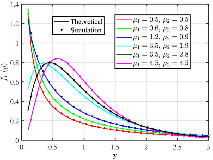
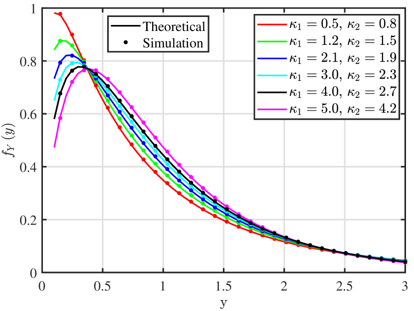
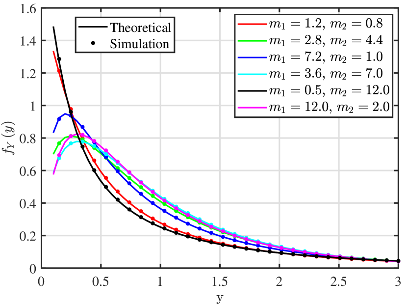
This section presents the simulation results that show the correctness and utility of the theoretical expression presented in the previous sections. Without loss of generality, we have assumed γ¯1=γ¯2=1subscript¯𝛾1subscript¯𝛾21\bar{\gamma}_{1}=\bar{\gamma}_{2}=1 for all the plots. In all the figures, We have used solid lines to draw the theoretical values and the dotted markers are used for simulated values. In Figs. 2-4, several plots for the product PDF of two κμ𝜅𝜇\kappa-\mu shadowed RV for various values of κ,μ𝜅𝜇\kappa,\mu and m𝑚m. A wide range of shapes can be obtained via choosing different parameter as confirmed by the Figs. 2-4. Also, one can observe that the simulated PDFs are perfectly matching with the values obtained through theoretical expressions in (12) or (16) when the difference of μ2subscript𝜇2\mu_{2} and μ1subscript𝜇1\mu_{1} is an integer. It validates the exactness of series expression.
Refer to caption
Figure 1: PDF of Y𝑌Y with {κ1,μ1}={5.0,1.2}subscript𝜅1subscript𝜇15.01.2\{\kappa_{1},\mu_{1}\}=\{5.0,1.2\} , {κ2,μ2}={2.1,3.0}subscript𝜅2subscript𝜇22.13.0\{\kappa_{2},\mu_{2}\}=\{2.1,3.0\} and various values of m1subscript𝑚1m_{1} and m2subscript𝑚2m_{2}
Refer to caption
Figure 2: PDF of Y𝑌Y with {κ1,m1}={2.2,10}subscript𝜅1subscript𝑚12.210\{\kappa_{1},m_{1}\}=\{2.2,10\} , {κ2,m2}={0.9,4.0}subscript𝜅2subscript𝑚20.94.0\{\kappa_{2},m_{2}\}=\{0.9,4.0\} and various values of μ1subscript𝜇1\mu_{1} and μ2subscript𝜇2\mu_{2}
Refer to caption
Figure 3: PDF of Y𝑌Y with {μ1,m1}={2.1,10}subscript𝜇1subscript𝑚12.110\{\mu_{1},m_{1}\}=\{2.1,10\} , {μ2,m2}={1.5,4.0}subscript𝜇2subscript𝑚21.54.0\{\mu_{2},m_{2}\}=\{1.5,4.0\} and various values of κ1subscript𝜅1\kappa_{1} and κ2subscript𝜅2\kappa_{2}
Refer to caption
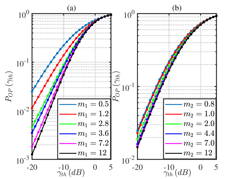
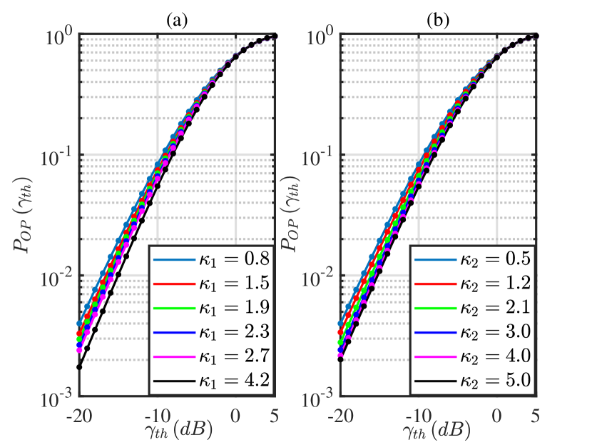
Figure 4: OP of cascaded κμ𝜅𝜇\kappa-\mu shadowed channel with {κ1,μ1}={5.0,1.2}subscript𝜅1subscript𝜇15.01.2\{\kappa_{1},\mu_{1}\}=\{5.0,1.2\} , {κ2,μ2}={2.1,3.0}subscript𝜅2subscript𝜇22.13.0\{\kappa_{2},\mu_{2}\}=\{2.1,3.0\} and various values of m1subscript𝑚1m_{1} and m2subscript𝑚2m_{2}

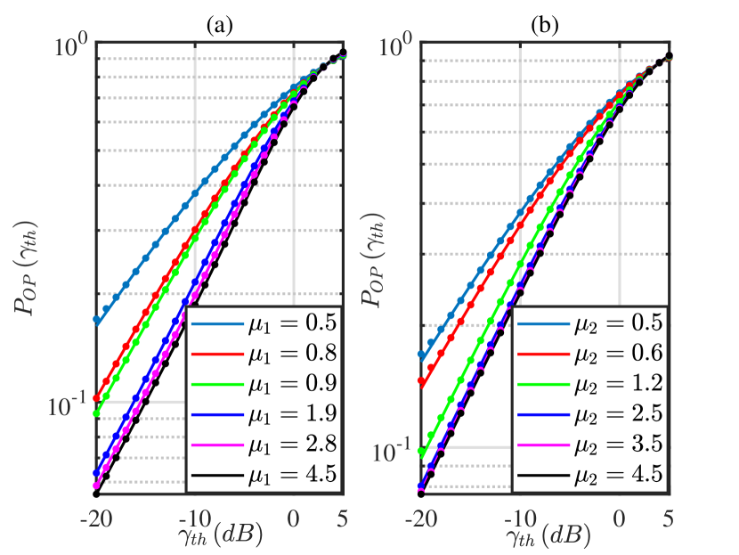
Next, we studied the effect of individual parameters on the OP of a cascaded κμ𝜅𝜇\kappa-\mu shadowed fading channel. Fig. 4 shows the impact of increasing the m𝑚m parameter of single link when all other parameters are kept constant. In Fig 4(a), we kept κ1=5.0,μ1=1.2formulae-sequencesubscript𝜅15.0subscript𝜇11.2\kappa_{1}=5.0,\mu_{1}=1.2 and κ2=2.1,μ2=3.0,m2=0.8formulae-sequencesubscript𝜅22.1formulae-sequencesubscript𝜇23.0subscript𝑚20.8\kappa_{2}=2.1,\mu_{2}=3.0,m_{2}=0.8 then we changed the value of m1subscript𝑚1m_{1}. Similarly in Fig. 4(b) we kept κ1=5.0,μ1=1.2,m1=0.5formulae-sequencesubscript𝜅15.0formulae-sequencesubscript𝜇11.2subscript𝑚10.5\kappa_{1}=5.0,\mu_{1}=1.2,m_{1}=0.5 and κ2=2.1,μ2=3.0formulae-sequencesubscript𝜅22.1subscript𝜇23.0\kappa_{2}=2.1,\mu_{2}=3.0 then we changed the value of m2subscript𝑚2m_{2}. It can be observed that as m𝑚m increases the OP decreases but the effect is not independent of other parameter as in Fig. 4(a) the impact of increasing m𝑚m is more dominant compare to Fig. 4(b) where it saturates for m2=4.4subscript𝑚24.4m_{2}=4.4 only. One reason for this behavior may be that the κ1>κ2subscript𝜅1subscript𝜅2\kappa_{1}>\kappa_{2} and dominates the overall link. We fixed all the parameter except μ1subscript𝜇1\mu_{1} and μ2subscript𝜇2\mu_{2} in 6(a) and 6(b), respectively. Again, we can conclude that as μ𝜇\mu increases the OP decreases. In other words, a fading channel with higher μ𝜇\mu is more reliable. In the same way, the impact of κ𝜅\kappa has been demonstrated in Fig. 6.

Refer to caption
Figure 5: OP of cascaded κμ𝜅𝜇\kappa-\mu shadowed channel with {κ1,m1}={0.9,4}subscript𝜅1subscript𝑚10.94\{\kappa_{1},m_{1}\}=\{0.9,4\} , {κ2,m2}={2.2,10}subscript𝜅2subscript𝑚22.210\{\kappa_{2},m_{2}\}=\{2.2,10\} and various values of μ1subscript𝜇1\mu_{1} and μ2subscript𝜇2\mu_{2}
Refer to caption
Figure 6: OP of cascaded κμ𝜅𝜇\kappa-\mu shadowed channel with {μ1,m1}={1.5,4}subscript𝜇1subscript𝑚11.54\{\mu_{1},m_{1}\}=\{1.5,4\} , {μ2,m2}={2.1,10}subscript𝜇2subscript𝑚22.110\{\mu_{2},m_{2}\}=\{2.1,10\} and various values of κ1subscript𝜅1\kappa_{1} and κ2subscript𝜅2\kappa_{2}
Refer to caption
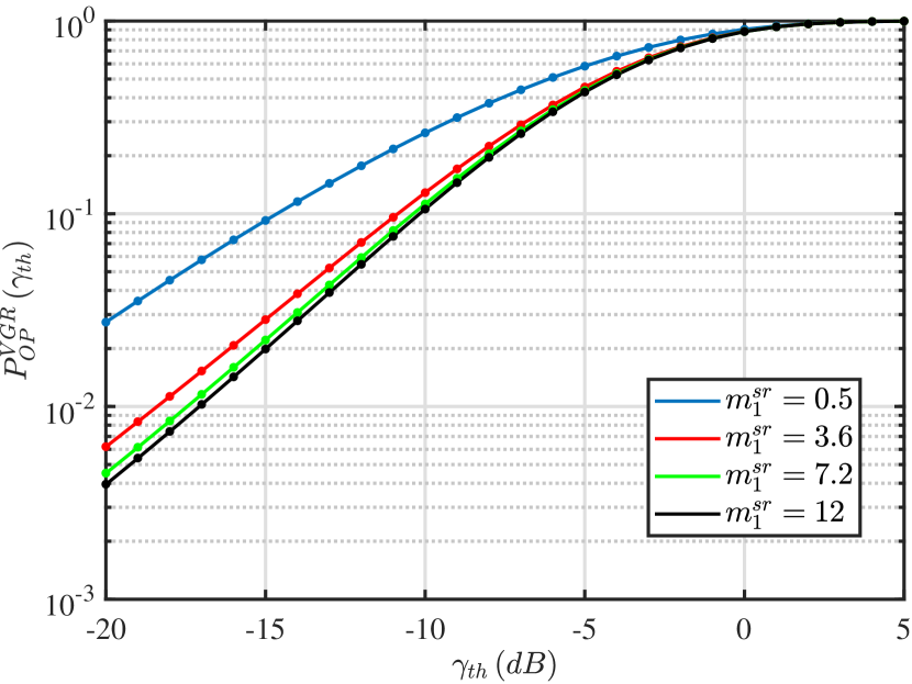
Figure 7: OP for variable relay gain with κμ𝜅𝜇\kappa-\mu shadowed fading for various m1srsuperscriptsubscript𝑚1𝑠𝑟m_{1}^{sr}
Refer to caption
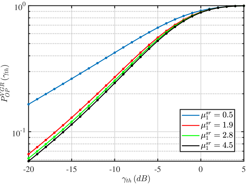
Figure 8: OP for variable relay gain with κμ𝜅𝜇\kappa-\mu shadowed fading for various μ1srsuperscriptsubscript𝜇1𝑠𝑟\mu_{1}^{sr}

Next, in Fig. 8 and 8 we plotted the OP for the relay-assisted wireless communication system with variable gain relay to validate the expression in (32). These figures re-validate the exactness of formulation as the simulated and theoretical values match perfectly. Here, also one can observe that with the increase in parameter values fading channel gets more reliable as the OP decreases.

V Conclusion

This paper presents the series expression for PDF, CDF, and MGF of the product of two κμ𝜅𝜇\kappa-\mu shadowed RV. The series expression is obtained via a direct application of Mellin transformation and can be easily computed using popular software like Mathematica. A couple of application examples are also provided for the considered cascaded fading channel. An interesting extension for this work can be to consider the product of an arbitrary number of κμ𝜅𝜇\kappa-\mu shadowed RVs.

Appendix A Evaluation of S2,nsubscript𝑆2𝑛S_{2,n}

S2,nsubscript𝑆2𝑛\displaystyle S_{2,n} =limsnμ1+1dds{(s+n+μ11)2Γ(s+μ11)Γ(s+μ21)(a1a2)s1F12(m1,s+μ11;μ1;c1)\displaystyle=\lim_{s\rightarrow-n-\mu_{1}+1}\frac{d}{ds}\Bigg{\{}\frac{\left(s+n+\mu_{1}-1\right)^{2}\Gamma\left(s+\mu_{1}-1\right)\Gamma\left(s+\mu_{2}-1\right)}{\left(a_{1}a_{2}\right)^{s-1}}{}_{2}F_{1}\left(m_{1},s+\mu_{1}-1;\mu_{1};c_{1}\right) (33)
×F12(m2,s+μ21;μ2;c2)ys}\displaystyle\times{}_{2}F_{1}\left(m_{2},s+\mu_{2}-1;\mu_{2};c_{2}\right)y^{-s}\Bigg{\}}
=limsnμ1+1{ϕ(s)h(s)+ϕ(s)h(s)}absentsubscript𝑠𝑛subscript𝜇11superscriptitalic-ϕ𝑠𝑠italic-ϕ𝑠superscript𝑠\displaystyle=\lim_{s\rightarrow-n-\mu_{1}+1}\left\{\phi^{\prime}\left(s\right)h\left(s\right)+\phi\left(s\right)h^{\prime}\left(s\right)\right\}
=(limsnμ1+1ϕ(s))(limsnμ1+1h(s))+(limsnμ1+1ϕ(s))(limsnμ1+1h(s))absentsubscript𝑠𝑛subscript𝜇11superscriptitalic-ϕ𝑠subscript𝑠𝑛subscript𝜇11𝑠subscript𝑠𝑛subscript𝜇11italic-ϕ𝑠subscript𝑠𝑛subscript𝜇11superscript𝑠\displaystyle=\left(\lim_{s\rightarrow-n-\mu_{1}+1}\phi^{\prime}\left(s\right)\right)\left(\lim_{s\rightarrow-n-\mu_{1}+1}h\left(s\right)\right)+\left(\lim_{s\rightarrow-n-\mu_{1}+1}\phi\left(s\right)\right)\left(\lim_{s\rightarrow-n-\mu_{1}+1}h^{\prime}\left(s\right)\right)

where,

ϕ(s)italic-ϕ𝑠\displaystyle\phi\left(s\right) =(s+n+μ11)2Γ(s+μ11)Γ(s+μ21)absentsuperscript𝑠𝑛subscript𝜇112Γ𝑠subscript𝜇11Γ𝑠subscript𝜇21\displaystyle=\left(s+n+\mu_{1}-1\right)^{2}\Gamma\left(s+\mu_{1}-1\right)\Gamma\left(s+\mu_{2}-1\right) (34)

and

h(s)𝑠\displaystyle h\left(s\right) =1(a1a2)s1F12(m1,s+μ11;μ1;c1)F12(m2,s+μ21;μ2;c2)ysabsent1superscriptsubscript𝑎1subscript𝑎2𝑠1subscriptsubscript𝐹12subscript𝑚1𝑠subscript𝜇11subscript𝜇1subscript𝑐1subscriptsubscript𝐹12subscript𝑚2𝑠subscript𝜇21subscript𝜇2subscript𝑐2superscript𝑦𝑠\displaystyle=\frac{1}{\left(a_{1}a_{2}\right)^{s-1}}{}_{2}F_{1}\left(m_{1},s+\mu_{1}-1;\mu_{1};c_{1}\right){}_{2}F_{1}\left(m_{2},s+\mu_{2}-1;\mu_{2};c_{2}\right)y^{-s} (35)

Following the procedure as described in [41], we can rewrite ϕ(s)italic-ϕ𝑠\phi\left(s\right) as

ϕ(s)italic-ϕ𝑠\displaystyle\phi\left(s\right) =Γ2(s+μ1+n)(s+μ1+n2)2(s+μ11+N)2(s+μ1+N2)(s+μ11)absentsuperscriptΓ2𝑠subscript𝜇1𝑛superscript𝑠subscript𝜇1𝑛22superscript𝑠subscript𝜇11𝑁2𝑠subscript𝜇1𝑁2𝑠subscript𝜇11\displaystyle=\frac{\Gamma^{2}\left(s+\mu_{1}+n\right)}{\left(s+\mu_{1}+n-2\right)^{2}\dots\left(s+\mu_{1}-1+N\right)^{2}\left(s+\mu_{1}+N-2\right)\dots\left(s+\mu_{1}-1\right)} (36)

From (36), we have

limsnμ1+1ϕ(s)subscript𝑠𝑛subscript𝜇11italic-ϕ𝑠\displaystyle\lim_{s\rightarrow-n-\mu_{1}+1}\phi\left(s\right) =(1)N(nN)!n!absentsuperscript1𝑁𝑛𝑁𝑛\displaystyle=\frac{\left(-1\right)^{N}}{\left(n-N\right)!n!} (37)

To compute the ϕ(s)superscriptitalic-ϕ𝑠\phi^{\prime}\left(s\right), we take the logarithmic derivative i.e.,

ϕ(s)superscriptitalic-ϕ𝑠\displaystyle\phi^{\prime}\left(s\right) =ϕ(s)ddsln(ϕ(s))absentitalic-ϕ𝑠𝑑𝑑𝑠italic-ϕ𝑠\displaystyle=\phi\left(s\right)\frac{d}{ds}\ln\left(\phi\left(s\right)\right) (38)

After some algebraic manipulations, we get

ddsln(ϕ(s))𝑑𝑑𝑠italic-ϕ𝑠\displaystyle\frac{d}{ds}\ln\left(\phi\left(s\right)\right) =2ψ(s+μ1+n)2(s+μ1+n2)2(s+μ1+N1)absent2𝜓𝑠subscript𝜇1𝑛2𝑠subscript𝜇1𝑛22𝑠subscript𝜇1𝑁1\displaystyle=2\psi\left(s+\mu_{1}+n\right)-\frac{2}{\left(s+\mu_{1}+n-2\right)}-\dots-\frac{2}{\left(s+\mu_{1}+N-1\right)} (39)
1(s+μ1+N2)1(s+μ11).1𝑠subscript𝜇1𝑁21𝑠subscript𝜇11\displaystyle-\frac{1}{\left(s+\mu_{1}+N-2\right)}-\dots-\frac{1}{\left(s+\mu_{1}-1\right)}.
limsnμ1+1ddsln(ϕ(s))subscript𝑠𝑛subscript𝜇11𝑑𝑑𝑠italic-ϕ𝑠\displaystyle\lim_{s\rightarrow-n-\mu_{1}+1}\frac{d}{ds}\ln\left(\phi\left(s\right)\right) =2ψ(1)+2(1+12++1nN)+(1nN+1++1n)absent2𝜓121121𝑛𝑁1𝑛𝑁11𝑛\displaystyle=2\psi\left(1\right)+2\left(1+\frac{1}{2}+\dots+\frac{1}{n-N}\right)+\left(\frac{1}{n-N+1}+\dots+\frac{1}{n}\right) (40)

By using [41, Eq. 1.4.6], we have

limsnμ1+1ddsln(ϕ(s))subscript𝑠𝑛subscript𝜇11𝑑𝑑𝑠italic-ϕ𝑠\displaystyle\lim_{s\rightarrow-n-\mu_{1}+1}\frac{d}{ds}\ln\left(\phi\left(s\right)\right) =ψ(n+1)+ψ(nN+1)absent𝜓𝑛1𝜓𝑛𝑁1\displaystyle=\psi\left(n+1\right)+\psi\left(n-N+1\right) (41)

After substituting (37) and (41) in (38), we get

limsnμ1+1ϕ(s)subscript𝑠𝑛subscript𝜇11superscriptitalic-ϕ𝑠\displaystyle\lim_{s\rightarrow-n-\mu_{1}+1}\phi^{\prime}\left(s\right) =(1)N(nN)!n![ψ(n+1)+ψ(nN+1)]absentsuperscript1𝑁𝑛𝑁𝑛delimited-[]𝜓𝑛1𝜓𝑛𝑁1\displaystyle=\frac{\left(-1\right)^{N}}{\left(n-N\right)!n!}\left[\psi\left(n+1\right)+\psi\left(n-N+1\right)\right] (42)

As h(s)𝑠h\left(s\right) is analytic function so we can simply substitute s=nμ1+1𝑠𝑛subscript𝜇11s=-n-\mu_{1}+1 to get

limsnμ1+1h(s)subscript𝑠𝑛subscript𝜇11𝑠\displaystyle\lim_{s\rightarrow-n-\mu_{1}+1}h\left(s\right) =yn+μ11(a1a2)n+μ1F12(m1,n;μ1;c1)F12(m2,n+N;μ2;c2)absentsuperscript𝑦𝑛subscript𝜇11superscriptsubscript𝑎1subscript𝑎2𝑛subscript𝜇1subscriptsubscript𝐹12subscript𝑚1𝑛subscript𝜇1subscript𝑐1subscriptsubscript𝐹12subscript𝑚2𝑛𝑁subscript𝜇2subscript𝑐2\displaystyle=y^{n+\mu_{1}-1}\left(a_{1}a_{2}\right)^{n+\mu_{1}}{}_{2}F_{1}\left(m_{1},-n;\mu_{1};c_{1}\right){}_{2}F_{1}\left(m_{2},-n+N;\mu_{2};c_{2}\right) (43)

Now, after taking the derivative of h(s)𝑠h\left(s\right) and substituting the s=nμ1+1𝑠𝑛subscript𝜇11s=-n-\mu_{1}+1, we get

limsnμ1+1h(s)subscript𝑠𝑛subscript𝜇11superscript𝑠\displaystyle\lim_{s\rightarrow-n-\mu_{1}+1}h^{\prime}\left(s\right) =F1(0,1,0,0)2(m1,n;μ1;c1)F12(m2,n+N;μ2;c2)(a1a2)n+μ1yn+μ11absentsubscriptsuperscriptsubscript𝐹101002subscript𝑚1𝑛subscript𝜇1subscript𝑐1subscriptsubscript𝐹12subscript𝑚2𝑛𝑁subscript𝜇2subscript𝑐2superscriptsubscript𝑎1subscript𝑎2𝑛subscript𝜇1superscript𝑦𝑛subscript𝜇11\displaystyle={}_{2}F_{1}^{\left(0,1,0,0\right)}\left(m_{1},-n;\mu_{1};c_{1}\right){}_{2}F_{1}\left(m_{2},-n+N;\mu_{2};c_{2}\right)\left(a_{1}a_{2}\right)^{n+\mu_{1}}y^{n+\mu_{1}-1} (44)
+F1(0,1,0,0)2(m2,n+N;μ2;c2)F12(m1,n;μ1;c1)(a1a2)n+μ1yn+μ11subscriptsuperscriptsubscript𝐹101002subscript𝑚2𝑛𝑁subscript𝜇2subscript𝑐2subscriptsubscript𝐹12subscript𝑚1𝑛subscript𝜇1subscript𝑐1superscriptsubscript𝑎1subscript𝑎2𝑛subscript𝜇1superscript𝑦𝑛subscript𝜇11\displaystyle+{}_{2}F_{1}^{\left(0,1,0,0\right)}\left(m_{2},-n+N;\mu_{2};c_{2}\right){}_{2}F_{1}\left(m_{1},-n;\mu_{1};c_{1}\right)\left(a_{1}a_{2}\right)^{n+\mu_{1}}y^{n+\mu_{1}-1}
ln(a1a2)F12(m1,n;μ1;c1)F12(m2,n+N;μ2;c2)(a1a2)n+μ1yn+μ11subscript𝑎1subscript𝑎2subscriptsubscript𝐹12subscript𝑚1𝑛subscript𝜇1subscript𝑐1subscriptsubscript𝐹12subscript𝑚2𝑛𝑁subscript𝜇2subscript𝑐2superscriptsubscript𝑎1subscript𝑎2𝑛subscript𝜇1superscript𝑦𝑛subscript𝜇11\displaystyle-\ln\left(a_{1}a_{2}\right){}_{2}F_{1}\left(m_{1},-n;\mu_{1};c_{1}\right){}_{2}F_{1}\left(m_{2},-n+N;\mu_{2};c_{2}\right)\left(a_{1}a_{2}\right)^{n+\mu_{1}}y^{n+\mu_{1}-1}
ln(y)F12(m1,n;μ1;c1)F12(m2,n+N;μ2;c2)(a1a2)n+μ1yn+μ11𝑦subscriptsubscript𝐹12subscript𝑚1𝑛subscript𝜇1subscript𝑐1subscriptsubscript𝐹12subscript𝑚2𝑛𝑁subscript𝜇2subscript𝑐2superscriptsubscript𝑎1subscript𝑎2𝑛subscript𝜇1superscript𝑦𝑛subscript𝜇11\displaystyle-\ln\left(y\right){}_{2}F_{1}\left(m_{1},-n;\mu_{1};c_{1}\right){}_{2}F_{1}\left(m_{2},-n+N;\mu_{2};c_{2}\right)\left(a_{1}a_{2}\right)^{n+\mu_{1}}y^{n+\mu_{1}-1}

Finally,

S2,nsubscript𝑆2𝑛\displaystyle S_{2,n} =(1)N(a1a2)n+μ1yn+μ11(nN)!n!{F1(0,1,0,0)2(m1,n;μ1;c1)F12(m2,n+N;μ2;c2)\displaystyle=\frac{\left(-1\right)^{N}\left(a_{1}a_{2}\right)^{n+\mu_{1}}y^{n+\mu_{1}-1}}{\left(n-N\right)!n!}\Bigg{\{}{}_{2}F_{1}^{\left(0,1,0,0\right)}\left(m_{1},-n;\mu_{1};c_{1}\right){}_{2}F_{1}\left(m_{2},-n+N;\mu_{2};c_{2}\right) (45)
+F12(m1,n;μ1;c1)F1(0,1,0,0)2(m2,n+N;μ2;c2)subscriptsubscript𝐹12subscript𝑚1𝑛subscript𝜇1subscript𝑐1subscriptsuperscriptsubscript𝐹101002subscript𝑚2𝑛𝑁subscript𝜇2subscript𝑐2\displaystyle+{}_{2}F_{1}\left(m_{1},-n;\mu_{1};c_{1}\right){}_{2}F_{1}^{\left(0,1,0,0\right)}\left(m_{2},-n+N;\mu_{2};c_{2}\right)
+[ψ(n+1)+ψ(nN+1)ln(y)ln(a1a2)]F12(m1,n;μ1;c1)F12(m2,n+N;μ2;c2)}.\displaystyle+\left[\psi\left(n+1\right)+\psi\left(n-N+1\right)-\ln\left(y\right)-\ln\left(a_{1}a_{2}\right)\right]{}_{2}F_{1}\left(m_{1},-n;\mu_{1};c_{1}\right){}_{2}F_{1}\left(m_{2},-n+N;\mu_{2};c_{2}\right)\Bigg{\}}.

Appendix B Calculation of AF

From the definition of AF in (26), we have

AF𝐴𝐹\displaystyle AF =𝔼[Y2](𝔼[Y])21absent𝔼delimited-[]superscript𝑌2superscript𝔼delimited-[]𝑌21\displaystyle=\frac{\mathbb{E}\left[Y^{2}\right]}{\left(\mathbb{E}\left[Y\right]\right)^{2}}-1 (46)

We have 𝔼[Y]=γ¯1γ¯2𝔼delimited-[]𝑌subscript¯𝛾1subscript¯𝛾2\mathbb{E}\left[Y\right]=\bar{\gamma}_{1}\bar{\gamma}_{2} and

𝔼[Y2]𝔼delimited-[]superscript𝑌2\displaystyle\mathbb{E}\left[Y^{2}\right] =b1b2(μ1)2(μ2)2(a1a2)2F12(m1,μ1+2;μ1;c1)F12(m2,μ2+2;μ2;c2)absentsubscript𝑏1subscript𝑏2subscriptsubscript𝜇12subscriptsubscript𝜇22superscriptsubscript𝑎1subscript𝑎22subscriptsubscript𝐹12subscript𝑚1subscript𝜇12subscript𝜇1subscript𝑐1subscriptsubscript𝐹12subscript𝑚2subscript𝜇22subscript𝜇2subscript𝑐2\displaystyle=\frac{b_{1}b_{2}\left(\mu_{1}\right)_{2}\left(\mu_{2}\right)_{2}}{\left(a_{1}a_{2}\right)^{2}}{}_{2}F_{1}\left(m_{1},\mu_{1}+2;\mu_{1};c_{1}\right){}_{2}F_{1}\left(m_{2},\mu_{2}+2;\mu_{2};c_{2}\right) (47)

Using the Euler transformation from [42, Eq. 1.2.2.2], we have

F12(m1,μ1+2;μ1;c1)subscriptsubscript𝐹12subscript𝑚1subscript𝜇12subscript𝜇1subscript𝑐1\displaystyle{}_{2}F_{1}\left(m_{1},\mu_{1}+2;\mu_{1};c_{1}\right) =1(1c1)m1F12(m1,2;μ1;c1c11)absent1superscript1subscript𝑐1subscript𝑚1subscriptsubscript𝐹12subscript𝑚12subscript𝜇1subscript𝑐1subscript𝑐11\displaystyle=\frac{1}{\left(1-c_{1}\right)^{m_{1}}}{}_{2}F_{1}\left(m_{1},-2;\mu_{1};\frac{c_{1}}{c_{1}-1}\right) (48)
=(1c1)m1[12m1μ1c1c11+m1(m1+1)μ1(μ1+1)(c1c11)2]absentsuperscript1subscript𝑐1subscript𝑚1delimited-[]12subscript𝑚1subscript𝜇1subscript𝑐1subscript𝑐11subscript𝑚1subscript𝑚11subscript𝜇1subscript𝜇11superscriptsubscript𝑐1subscript𝑐112\displaystyle=\left(1-c_{1}\right)^{-m_{1}}\left[1-\frac{2m_{1}}{\mu_{1}}\frac{c_{1}}{c_{1}-1}+\frac{m_{1}\left(m_{1}+1\right)}{\mu_{1}\left(\mu_{1}+1\right)}\left(\frac{c_{1}}{c_{1}-1}\right)^{2}\right]
=1b1[1+2κ1+μ1(m1+1)m1(μ1+1)κ12]absent1subscript𝑏1delimited-[]12subscript𝜅1subscript𝜇1subscript𝑚11subscript𝑚1subscript𝜇11superscriptsubscript𝜅12\displaystyle=\frac{1}{b_{1}}\left[1+2\kappa_{1}+\frac{\mu_{1}\left(m_{1}+1\right)}{m_{1}\left(\mu_{1}+1\right)}\kappa_{1}^{2}\right]
𝔼[Y2]𝔼delimited-[]superscript𝑌2\displaystyle\mathbb{E}\left[Y^{2}\right] =(μ1)2(μ2)2(a1a2)2[1+2κ1+μ1(m1+1)m1(μ1+1)κ12][1+2κ2+μ2(m2+1)m2(μ2+1)κ22]absentsubscriptsubscript𝜇12subscriptsubscript𝜇22superscriptsubscript𝑎1subscript𝑎22delimited-[]12subscript𝜅1subscript𝜇1subscript𝑚11subscript𝑚1subscript𝜇11superscriptsubscript𝜅12delimited-[]12subscript𝜅2subscript𝜇2subscript𝑚21subscript𝑚2subscript𝜇21superscriptsubscript𝜅22\displaystyle=\frac{\left(\mu_{1}\right)_{2}\left(\mu_{2}\right)_{2}}{\left(a_{1}a_{2}\right)^{2}}\left[1+2\kappa_{1}+\frac{\mu_{1}\left(m_{1}+1\right)}{m_{1}\left(\mu_{1}+1\right)}\kappa_{1}^{2}\right]\left[1+2\kappa_{2}+\frac{\mu_{2}\left(m_{2}+1\right)}{m_{2}\left(\mu_{2}+1\right)}\kappa_{2}^{2}\right] (49)
𝔼[Y2](𝔼[Y])2𝔼delimited-[]superscript𝑌2superscript𝔼delimited-[]𝑌2\displaystyle\frac{\mathbb{E}\left[Y^{2}\right]}{\left(\mathbb{E}\left[Y\right]\right)^{2}} =(μ1+1)(μ2+1)μ1μ2(κ1+1)2(κ2+1)2[1+2κ1+μ1(m1+1)m1(μ1+1)κ12][1+2κ2+μ2(m2+1)m2(μ2+1)κ22]absentsubscript𝜇11subscript𝜇21subscript𝜇1subscript𝜇2superscriptsubscript𝜅112superscriptsubscript𝜅212delimited-[]12subscript𝜅1subscript𝜇1subscript𝑚11subscript𝑚1subscript𝜇11superscriptsubscript𝜅12delimited-[]12subscript𝜅2subscript𝜇2subscript𝑚21subscript𝑚2subscript𝜇21superscriptsubscript𝜅22\displaystyle=\frac{\left(\mu_{1}+1\right)\left(\mu_{2}+1\right)}{\mu_{1}\mu_{2}\left(\kappa_{1}+1\right)^{2}\left(\kappa_{2}+1\right)^{2}}\left[1+2\kappa_{1}+\frac{\mu_{1}\left(m_{1}+1\right)}{m_{1}\left(\mu_{1}+1\right)}\kappa_{1}^{2}\right]\left[1+2\kappa_{2}+\frac{\mu_{2}\left(m_{2}+1\right)}{m_{2}\left(\mu_{2}+1\right)}\kappa_{2}^{2}\right] (50)

Finally, the substitution of (50) in (46) and some algebraic manipulation results in (27) and completes the proof.

References

  • [1] M.-S. Alouini and M. K. Simon, “Dual diversity over correlated log-normal fading channels,” IEEE Transactions on Communications, vol. 50, no. 12, pp. 1946–1959, 2002.
  • [2] A. Abdi and M. Kaveh, “On the utility of gamma pdf in modeling shadow fading (slow fading),” in 1999 IEEE 49th Vehicular Technology Conference (Cat. No. 99CH36363), vol. 3.   IEEE, 1999, pp. 2308–2312.
  • [3] M. D. Yacoub, “The κ𝜅\kappa-μ𝜇\mu distribution and the η𝜂\eta-μ𝜇\mu distribution,” IEEE Antennas and Propagation Magazine, vol. 49, no. 1, pp. 68–81, 2007.
  • [4] M. D. Yacoub, “The αμ𝛼𝜇\alpha-\mu distribution: A physical fading model for the stacy distribution,” IEEE Transactions on Vehicular Technology, vol. 56, no. 1, pp. 27–34, 2007.
  • [5] J. F. Paris, “Statistical characterization of κμ𝜅𝜇\kappa-\mu shadowed fading,” IEEE Transactions on Vehicular Technology, vol. 63, no. 2, pp. 518–526, 2013.
  • [6] F. J. Lopez-Martinez, J. F. Paris, and J. M. Romero-Jerez, “The κμ𝜅𝜇\kappa-\mu shadowed fading model with integer fading parameters,” IEEE Transactions on Vehicular Technology, vol. 66, no. 9, pp. 7653–7662, 2017.
  • [7] B. Talha and M. Paetzold, “Channel models for mobile-to-mobile cooperative communication systems: A state of the art review,” IEEE Vehicular Technology Magazine, vol. 6, no. 2, pp. 33–43, 2011.
  • [8] M. Di Renzo, A. Zappone, M. Debbah, M. S. Alouini, C. Yuen, J. de Rosny, and S. Tretyakov, “Smart radio environments empowered by reconfigurable intelligent surfaces: How it works, state of research, and the road ahead,” IEEE Journal on Selected Areas in Communications, vol. 38, no. 11, pp. 2450–2525, 2020.
  • [9] Q. Wu and R. Zhang, “Towards smart and reconfigurable environment: Intelligent reflecting surface aided wireless network,” IEEE Communications Magazine, vol. 58, no. 1, pp. 106–112, 2019.
  • [10] Zhang, Jiayi and Björnson, Emil and Matthaiou, Michail and Ng, Derrick Wing Kwan and Yang, Hong and Love, David J., “Prospective Multiple Antenna Technologies for Beyond 5G,” IEEE Journal on Selected Areas in Communications, vol. 38, no. 8, pp. 1637–1660, 2020.
  • [11] N. Fasarakis-Hilliard, P. N. Alevizos, and A. Bletsas, “Coherent detection and channel coding for bistatic scatter radio sensor networking,” IEEE Transactions on Communications, vol. 63, no. 5, pp. 1798–1810, 2015.
  • [12] P. N. Alevizos, A. Bletsas, and G. N. Karystinos, “Noncoherent short packet detection and decoding for scatter radio sensor networking,” IEEE Transactions on Communications, vol. 65, no. 5, pp. 2128–2140, 2017.
  • [13] P. N. Alevizos, K. Tountas, and A. Bletsas, “Multistatic scatter radio sensor networks for extended coverage,” IEEE Transactions on Wireless Communications, vol. 17, no. 7, pp. 4522–4535, 2018.
  • [14] J. Salo, H. M. El-Sallabi, and P. Vainikainen, “The distribution of the product of independent Rayleigh random variables,” IEEE Transactions on Antennas and Propagation, vol. 54, no. 2, pp. 639–643, 2006.
  • [15] G. K. Karagiannidis, N. C. Sagias, and P. T. Mathiopoulos, “N{N}\ast Nakagami: a novel stochastic model for cascaded fading channels,” IEEE Transactions on Communications, vol. 55, no. 8, pp. 1453–1458, 2007.
  • [16] F. Yilmaz and M.-S. Alouini, “Product of the powers of generalized nakagami-m variates and performance of cascaded fading channels,” in GLOBECOM 2009-2009 IEEE Global Telecommunications Conference.   IEEE, 2009, pp. 1–8.
  • [17] N. Bhargav, C. R. N. da Silva, Y. J. Chun, E. J. Leonardo, S. L. Cotton, and M. D. Yacoub, “On the product of two κ𝜅\kappa-μ𝜇\mu random variables and its application to double and composite fading channels,” IEEE Transactions on Wireless Communications, vol. 17, no. 4, pp. 2457–2470, 2018.
  • [18] C. R. N. da Silva, E. J. Leonardo, and M. D. Yacoub, “Product of two envelopes taken from α𝛼\alpha - μ𝜇\mu , κ𝜅\kappa - μ𝜇\mu , and η𝜂\eta - μ𝜇\mu distributions,” IEEE Transactions on Communications, vol. 66, no. 3, pp. 1284–1295, 2018.
  • [19] M. Charishma, A. Subhash, S. Shekhar, and S. Kalyani, “Outage probability expressions for an irs-assisted system with and without source-destination link for the case of quantized phase shifts in κμ𝜅𝜇\kappa-\mu fading,” IEEE Transactions on Communications, pp. 1–1, 2021.
  • [20] S. Kumar, “Approximate outage probability and capacity for κμ𝜅𝜇\kappa-\mu shadowed fading,” IEEE Wireless Communications Letters, vol. 4, no. 3, pp. 301–304, 2015.
  • [21] S. Kumar and S. Kalyani, “Outage probability and rate for κμ𝜅𝜇\kappa-\mu shadowed fading in interference limited scenario,” IEEE Transactions on Wireless Communications, vol. 16, no. 12, pp. 8289–8304, 2017.
  • [22] G. Chandrasekaran and S. Kalyani, “Performance analysis of cooperative spectrum sensing over κμ𝜅𝜇\kappa-\mu shadowed fading,” IEEE Wireless Communications Letters, vol. 4, no. 5, pp. 553–556, 2015.
  • [23] M. R. Bhatnagar, “On the sum of correlated squared κμ𝜅𝜇\kappa-\mu shadowed random variables and its application to performance analysis of MRC,” IEEE Transactions on Vehicular Technology, vol. 64, no. 6, pp. 2678–2684, 2014.
  • [24] S. L. Cotton, “Second-order statistics of κμ𝜅𝜇\kappa-\mu shadowed fading channels,” IEEE Transactions on Vehicular Technology, vol. 65, no. 10, pp. 8715–8720, 2015.
  • [25] M. Srinivasan and S. Kalyani, “Secrecy capacity of κμ𝜅𝜇\kappa-\mu shadowed fading channels,” IEEE Communications Letters, vol. 22, no. 8, pp. 1728–1731, 2018.
  • [26] A. Subhash, M. Srinivasan, and S. Kalyani, “Asymptotic maximum order statistic for sir in κμ𝜅𝜇\kappa-\mu shadowed fading,” IEEE Transactions on Communications, vol. 67, no. 9, pp. 6512–6526, 2019.
  • [27] M. Bilim, “Cascaded double fading channels: A case of κμ𝜅𝜇\kappa-\mu shadowing,” Physical Communication, p. 101649, 2022.
  • [28] H. M. Srivastava and P. W. Karlsson, Multiple Gaussian hypergeometric series.   Ellis Horwood, 1985.
  • [29] I. S. Gradshteyn and I. M. Ryzhik, Table of integrals, series, and products.   Academic Press, 2007.
  • [30] M. D. Springer, The algebra of random variables.   New York: Wiley, 1979.
  • [31] E. W. Weisstein, Polygamma Function, (accessed Feb 12, 2022). [Online]. Available: https://mathworld.wolfram.com/PolygammaFunction.html
  • [32] E. W. Weisstein, Gauss Hypergeometric Function F12subscriptsubscript𝐹12{}_{2}F_{1}, (accessed Feb 12, 2022). [Online]. Available: http://functions.wolfram.com/07.23.20.0004.01
  • [33] J. B. Andersen, “Statistical distributions in mobile communications using multiple scattering,” in Proc. 27th URSI General Assembly, 2002, pp. 1–4.
  • [34] V. Erceg, S. J. Fortune, J. Ling, A. Rustako, and R. A. Valenzuela, “Comparisons of a computer-based propagation prediction tool with experimental data collected in urban microcellular environments,” IEEE Journal on Selected Areas in Communications, vol. 15, no. 4, pp. 677–684, 1997.
  • [35] J. Salo, H. M. El-Sallabi, and P. Vainikainen, “Statistical analysis of the multiple scattering radio channel,” IEEE Transactions on Antennas and Propagation, vol. 54, no. 11, pp. 3114–3124, 2006.
  • [36] D. Chizhik, G. J. Foschini, M. J. Gans, and R. A. Valenzuela, “Keyholes, correlations, and capacities of multielement transmit and receive antennas,” IEEE Transactions on Wireless Communications, vol. 1, no. 2, pp. 361–368, 2002.
  • [37] M. K. Simon and M.-S. Alouini, Digital communication over fading channels.   John Wiley & Sons, 2005, vol. 95.
  • [38] A. S. Lioumpas, G. K. Karagiannidis, and A. C. Iossifides, “Channel quality estimation index (CQEI): An improved performance criterion for wireless communications systems over fading channels,” in 12th European Wireless Conference 2006-Enabling Technologies for Wireless Multimedia Communications.   VDE, 2006, pp. 1–6.
  • [39] S. S. Ikki and S. Aissa, “Performance evaluation and optimization of dual-hop communication over Nakagamim𝑚-m fading channels in the presence of co-channel interferences,” IEEE Communications Letters, vol. 16, no. 8, pp. 1149–1152, 2012.
  • [40] E. Zedini, I. S. Ansari, and M.-S. Alouini, “Performance analysis of mixed Nakagamim𝑚-m and gamma–gamma dual-hop fso transmission systems,” IEEE Photonics Journal, vol. 7, no. 1, pp. 1–20, 2014.
  • [41] A. M. Mathai, A handbook of generalized special functions for statistical and physical sciences.   Oxford University Press, USA, 1993.
  • [42] H. Exton, Multiple hypergeometric functions and applications.   Ellis Horwood, 1976.