What’s the Difference? The potential for Convolutional Neural Networks for transient detection without template subtraction

Tatiana Acero-Cuellar University of Delaware, Department of Physics and Astronomy, Newark, DE USA Universidad Nacional de Colombia, Observatorio Astronómio Nacional, Bogotá, Colombia Federica Bianco University of Delaware, Department of Physics and Astronomy, Newark, DE USA University of Delaware, Joseph R. Biden, Jr. School of Public Policy and Administration, Newark, DE USA University of Delaware, Data Science Institute, Newark, DE, USA Vera C. Rubin Observatory, Tucson, AZ, USA Gregory Dobler University of Delaware, Joseph R. Biden, Jr. School of Public Policy and Administration, Newark, DE USA University of Delaware, Department of Physics and Astronomy, Newark, DE USA University of Delaware, Data Science Institute, Newark, DE, USA Masao Sako Department of Physics and Astronomy, University of Pennsylvania, Philadelphia, PA, USA Helen Qu Department of Physics and Astronomy, University of Pennsylvania, Philadelphia, PA, USA

Abstract

We present a study of the potential for Convolutional Neural Networks (CNNs) to enable separation of astrophysical transients from image artifacts, a task known as “real-bogus” classification without requiring a template subtracted (or difference) image which requires a computationally expensive process to generate, involving image matching on small spatial scales in large volumes of data. Using data from the Dark Energy Survey, we explore the use of CNNs to (1) automate the “real-bogus” classification, (2) reduce the computational costs of transient discovery. We compare the efficiency of two CNNs with similar architectures, one that uses “image triplets” (templates, search, and difference image) and one that takes as input the template and search only. We measure the decrease in efficiency associated with the loss of information in input finding that the testing accuracy is reduced from $\sim 96\%$ to $\sim 91.1\%$ . We further investigate how the latter model learns the required information from the template and search by exploring the saliency maps. Our work (1) confirms that CNNs are excellent models for “real-bogus” classification that rely exclusively on the imaging data and require no feature engineering task; (2) demonstrates that high-accuracy (>90%) models can be built without the need to construct difference images, but some accuracy is lost. Since once trained, neural networks can generate predictions at minimal computational costs, we argue that future implementations of this methodology could dramatically reduce the computational costs in the detection of transients in synoptic surveys like Rubin Observatory’s Legacy Survey of Space and Time by bypassing the Difference Image Analysis entirely.

1 Introduction

Modern observational astronomy has shown us that the Universe is not static and immutable: to the contrary, it is a lively and dynamic system. We now know and understand a variety of different phenomena that can give rise to variations in the brightness and color of astrophysical objects, including explosive stellar death (supernovae, kilonovae, Gamma Ray Bursts, etc), less dramatic and powerful stellar variability (flares, pulsations), and variability arising from geometric effects (such as planetary transients and microlensing). The time scales for these phenomena range from seconds to years. When the variations are terminal –like supernovae– or stochastic –like stellar flares– they are often referred to as “transients”. Detecting optical astrophysical transients characteristically requires sequences of images across a significant temporal baseline. Surveys designed to study the ever-changing skies, like the Dark Energy Survey (The Dark Energy Survey Collaboration, 2005, DES) or the future Rubin Observatory Legacy Survey of Space and Time (Ivezić et al., 2019, LSST) and many others, search for spatially localized changes in brightness in patches of sky previously observed.

Due to the rarity of astrophysical transients, a long baseline in conjunction with the observation of a large area of the sky is typically required to detect a statistically significant sample of transients like supernovae and individual examples of rare events, such as kilonovae. The process itself is arduous and requires considerable human intervention at multiple stages. The first step is typically the creation of high quality templates of each region of the sky that is to be searched; the templates are then subtracted from nightly images, a process known in astrophysics as Difference Image Analysis (DIA) that was initially pioneered by Crotts (1992) and Tomaney & Crotts (1996) and then formalized by Alard & Lupton (1998) and there is a rich history of subsequent improvements in the efficiency and accuracy of DIA models. Templates (tmpl) are typically constructed as stacks of high quality (favorable observing conditions) sky images. These high quality images must then be aligned with the “today” image, typically called the “search image” (srch), and degraded to match its Point Spread Function (PSF, which we note may vary across a single large field of view image) and scaled to match its brightness. The product generated by the subtraction of the template from the search image is the so-called “difference image” (diff; see for example a description of the DIA processing pipeline for DES in Kessler et al. 2015). Transients can then be detected as clusters of adjacent pixels deviating significantly from the background. However, even the best existing DIA algorithms produce difference images with large pixel value deviation from an ideal 0-average that would be expected if no changes occurred in a patch of sky. Transients, variable stars, and moving objects will result in detections, but also a typically large number of artifacts will be detected by these thresholding schemes.

Machine learning models offer an excellent opportunity to improve the efficiency of transient detection at this stage, automating the classification between “real” astrophysical transients and “bogus” artifacts: these models are often referred to as “Real-Bogus” (hereafter, RB). Generally, the applications of machine learning to this problem are based on the extraction of features from the (difference) images that are then fed to models like Random Forests, k-Nearest Neighbors, or Support Vector Machines (Goldstein et al., 2015; Sánchez et al., 2019; Mong et al., 2020). These models have achieved high accuracy and enabled the discovery of transients at scale in larger synoptic surveys, for example in the Palomar Transient Factory (PTF Bloom et al., 2012) and Zwicky Transient Facility (ZTF Mahabal et al., 2019).

The process of engineering features for machine learning models allows the experts to embed domain knowledge in models. In the case of RB classification, the features engineered to be used by models such as the ones described above usually rely on visual inspection of a subset of the data. However, these features may overlook abstract associations between image properties that can be effective for classification, and in fact, may be biased towards human perception and theoretical expectations. An alternative approach involves the use of models that can learn features directly from the data, such as Convolutional Neural Networks (LeCun et al., 1989, CNNs). Here, it is possible to train a model using the images themselves, skipping the step of feature-design entirely.

RB CNN-based models appeared in the literature as early as 2016 (Cabrera-Vives et al., 2016), and they are typically based on the analysis of the difference images arising from the DIA. While neural networks may be computationally demanding in the training phase, the "feed-forward" classification that arises from a pre-trained model is typically rapid and computationally light,¹¹1although the model may require a large amount of memory to cache. leaving DIA as the computational bottle-neck in the process of astrophysical transients’ detection. Yet in principle, the entirety of the information content embedded in the diff-tmpl-srch image triplet is also contained in the tmpl-srch image pair. In this paper, we explore the use of CNNs as RB models concentrating on the potential for building high-accuracy models that do not require the construction of difference images.

This paper represents a first, critical step in the process of conceptualizing and realizing a DIA-free model for astrophysical transients. Here we invesigate if Neural Networks can discriminate between astrophysical transients and artifacts without a difference image, while still relying on DIA for detection. This is the necessary premise for the complete elimination of DIA and estimating the impact of the information lost by dropping the diff will enable future work toward the development of models that will not rely on DIA for detection, and that will detect and characterize transients (measure magnitude) from the tmpl-srch image pair only.

This paper is organized as follows: in section 2 we discuss the DIA history and methodology. In section 3 we present the DES data that we used to build our RB classification models and the pre-processing steps. In section 4 we discuss our methodology, illustrating the CNNs architectures used and, in subsection 4.4, presenting and discussing the use of saliency maps to gain insights into the models. In section 5 we show the results of building a model that does not use the difference image as input, named noDIA-based-based model and compare its performance to one that does, named DIA-based model; we outline future work and conclude with a discussion of the broader implications for this result in light of upcoming surveys in section 6.

This study is reproducible and all the code that supports the analysis presented here is available on a dedicated GitHub repository.²²2https://github.com/taceroc/DIA_noDIA.

Refer to caption — Figure 1: Example of four DIA-sets from the first season of the Dark Energy Survey (DES): from left to right the images correspond to the template (tmpl), search (srch), and difference (diff) image; the diff is generated as the subtraction of tmpl and srch. Each pair of tmpl and srch images is mapped to the same color range. We refer to these 3-images sets as “image triplets” or DIA-sets. A and B show artifacts, human-labeled as “bogus” (label = 1). C and D show transients labeled as “real” (label = 0). Above each triplet is the unique ID of the transient (see Goldstein et al. 2015)

2 state of the art and traditional solutions to detection of transients

2.1 Difference Imaging

Difference images are produced subtracting a template, an image generated coadding multiple images (e.g. Kessler et al., 2015), from a sky image and they are currently the basis for most astrophysical transient search algorithms. The difference image allows brightness changes to be detected even if embedded in Galaxy light, for example, in the case of extra-galactic explosive transients. Great efforts have been made to improve the quality and effectiveness of the difference images. Although the name may suggest the process simply entails subtracting images from each other, the procedure is in fact riddled with complications because of the following reasons. First, the images used to build the template and the search images are taken principally within different atmospheric conditions (Zackay & Ofek, 2017) generating variations in the quality of the images. The construction of a proper template is also a delicate task; typically templates are built by stacking tens of images taken under favourable sky conditions at different times. This improves the image quality but also mitigates issues related to variability in the astrophysical objects captured in the image (Hambleton et al., 2020): one wants to capture each variable source at its representative brightness. Typically then, the template image is of higher quality than the search image, and it is degraded to match the search image PSF and scaled to match its brightness. Yet, the scaling and PSF may vary locally in the image plane, especially for images from large field of view synoptic surveys such as the 2.2 sq. degrees DES or $\sim 10$ sq. degrees Rubin images. Finally it is important that the images are perfectly aligned, both in the creation of the template and in the subtraction process to create the difference image. This implies accounting for rotation as well as potentially different warping effects on the images and template. Once the PSF match and the alignment is done, it is possible to subtract the degraded template from the search images to obtain the difference image. To degrade the image quality of the template to match the search image, a convolution kernel that must be applied to the template needs to be determined (Alard & Lupton, 1998),

\displaystyle\text{{\it tmpl}}(x,y)\otimes\text{Kernel}(u,v)=\text{{\it srch}}(x,y),

(1)

where tmpl is the high-quality image, the template image, srch is the one night image or search image and $\otimes$ is the convolutional operation. The arguments $x$ and $y$ represent the coordinates of the pixel matrix that compose the images; $u$ and $v$ the coordinates of the kernel matrix.

To solve the computationally expensive problem of matching PSFs, the kernel can be decomposed in terms of simple functions, for instance Gaussian functions, and the method of least squares can be used to determine the best values for the kernel. The fitted solution of one search image can be determined in a short computational time. However, the computational cost scales with the image size and resolution. Surveys and telescopes constructed with the goal of discovering new transients are generally designed to collect tremendous amounts of data to maximize event rate (detection of astrophysical transients). For the DES, the computational cost per 2.2 sq. degree image is $\sim 15.5$ CPU hours (with roughly 2/3 of that time spent on PSF matching)³³3 DES team, private communication.. The upcoming Rubin LSST will collect more than 500 images every night each with 3.2 Gigapixels. This process thus is bound to turn out to be very expensive. In this paper, we trained our models on postage stamps where transients were detected or simulated (see section 3), thus a direct comparison of the computational cost is not trivial. For comparison, a detailed discussion of the computational cost of our models is included in subsection 5.2 and the CPU Node hours required to train and generate predictions from our models are reported in Table 1. We note here that, with a Deep Neural Network approach to this problem, the computational cost is high in training, but the predictions require minimal computational time.

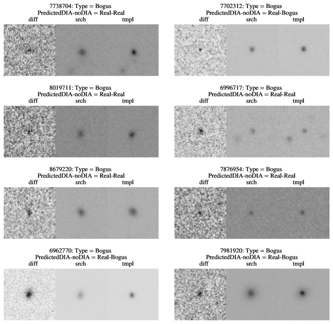
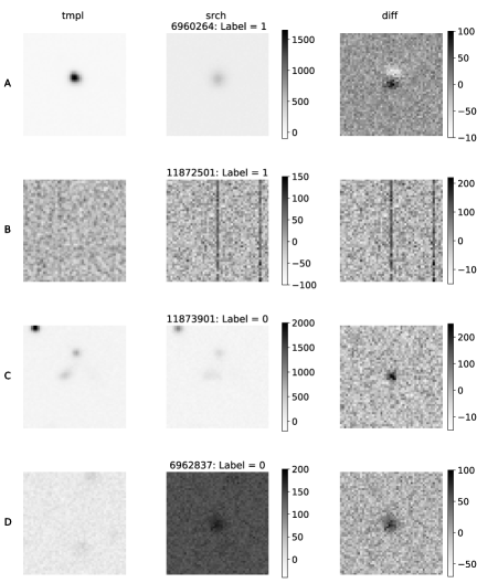
A bad subtraction can occur either because of poor PSF matching, poor alignment, or poor correction of image warping. In all of these cases, the subtraction would lead to artifacts or “bogus” alerts, like the one shown in the difference image in Figure 1A and B. In particular: in Figure 1A, the difference image shows a so-called “dipole”, where one side of a suspected transient is dark and the other side bright: this typically arises in case of mis-alignments, but it might also be caused by moving objects in the field, or differential chromatic refraction (Carrasco-Davis et al., 2021). Conversely, Figure 1B shows a “bogus” alert caused by an image artifact: a column of bad pixels in the search image. At this location there is no astrophysical object in the image thumbnail: no host galaxy or star that could give rise to variations.

Panels Figure 1C and Figure 1D show genuine transients in our DES training data: in both of these two examples, there is a clear transient in the diff images (high pixel values at the center of the image).

2.2 Autoscan and other feature-based Real Bogus models

We developed our models on data collected in the first year of DES. Thus, a direct precursor of our work is Goldstein et al. (2015), in which the authors created an automated RB based on a Random Forest (RF) supervised learning model (Ho, 1995) to detect transients, and particularly supernovae, in the DES data, hereafter refered to as autoscan. For these kinds of models, the process of selecting and engineering features is pivotal. Autoscan is based on 38 features derived from the diff, srch, and tmpl images. The selection and computation of these features was done attempting to represent quantitatively what humans would leverage in visual inspections. For instance, r_aper_psf distinguishes a bad subtraction of srch and tmpl that would lead to a diff qualitative similar to Figure 1A; the feature diffsum measures the significance of the detection by summing the pixel values in the center of the diff image; the feature colmeds, indicating the CCD used for the detection, is designed to identify artifacts specific of a CCD, like bad rows/columns of pixels.

In other RB models, like in Sánchez et al. (2019), the feature selection is performed purely statistically: features were initially selected based on variance thresholds. In the same work, different techniques are explored to reduce the number of features, and thus the complexity of the classification problem. For example, a RF model was trained using all features. Then a feature importance analysis enabled a reduction of the dimensionality of the problem by removing possible redundant or irrelevant features. Examples of models based on features closer to the data include Mong et al. (2020), where the features are simply the flux values of the pixels around the center of the image.

2.3 Deep Neural Netowrk approaches

CNNs have demonstrated enormous potential in image analysis including object detection, recognition, and classification across domains (Deng et al., 2009). Examples of astrophysics applications of CNNs include Dieleman et al. (2015) for galaxy morphology prediction, Kim & Brunner (2016) for star-galaxy classification, Gabbard et al. (2018) for signal/background separation for Gravitational Waves (GW) searches, where the GW time series are purposefully encoded as images to be analyzed by a CNN, and many more.

CNNs are particularly well-suited to learning discriminating features from image input data. CNNs can work on high dimensional spaces (here the dimensionality of the input is as large as the number of pixels in the image) due to the generalizability of the convolution operation to $n$ dimensions while preserving relative position information. Vectors of raw pixel values can theoretically be used to train traditionally feature-based models, such as RFs, but pixel-to-pixel position data in higher dimensions is unequivocally lost. Previous studies already compared feature-based supervised models, like RF, and supervised CNNs for RB, demonstrating that CNN s generally lead to increased accuracy. In Gieseke et al. (2017) an accuracy of $\sim 0.984$ is achieved with a RF model in the RB task, and it increases to $\sim 0.990$ when applying a CNNs to the same data. In Cabrera-Vives et al. (2016) an accuracy of $\sim 0.9889$ is achieved with a RF and is increased to $\sim 0.9932$ with a CNN. In Cabrera-Vives et al. (2017), an RF gave 0.9896 and a CNN 0.9945. In Liu et al. (2019) the accuracy improves from $\sim 0.9623$ with a RF to $\sim 0.9948$ with a CNN.

In Duev et al. (2019) a CNN RB classifier called braai, developed for the Zwicky Transient Facility (Bellm et al., 2018, ZTF), achieves a $\sim$ 98% accuracy for training and validation data set (Area Under the Curve, AUC = 0.99949). braai implementes a custom VGG16 (Simonyan & Zisserman, 2014) architecture.

Going beyond RB, a model for image-based transient classification through CNNs has been prototyped by the Automatic Learning for the Rapid Classification of Events team (ALeRCE Carrasco-Davis et al., 2021). The model classifies between AGNs (Active Galactic Nuclei), SNe (SuperNovae), variable stars, asteroids, and artifacts in ZTF (Bellm et al., 2018) survey data with a reported accuracy exceeding 95% for all types, except SNe (87%). This CNN model was trained using a combination of the srch, tmpl, and diff.

Here we explore the potential and the intricacies of leveraging AI to bypass the DIA step. The CNN RB models mentioned above differ not only in their architecture (for example, a single or multiple sequences of convolutional, pooling, dropout, and dense layers) but also in the choice of input. For instance, Gieseke et al. (2017) used the tmpl, srch, and diff images in combination for training their CNN; Cabrera-Vives et al. (2016) augmented this image set with an image generated as the diff divided by an estimate of the local noise; Cabrera-Vives et al. (2017) trained an ensemble of CNNs on different rotations of this four-fold image set. Conversely, Liu et al. (2019) used the diff as the sole input. Although, all these attempts have shown good results with accuracy higher than $90\%$ , these models all rely on DIA to construct the diff. Taking into account that diff are built from the tmpl and srch, and in principle, should carry no additional information content than the search-template pair alone, a logical step to follow would be to only consider the two latter images.

A first attempt in this direction is presented in Sedaghat & Mahabal (2018), where the authors develop a Convolutional Autoencoder (encoder-decoder) named TransiNet. The model is developed and tested on both real and synthetic data. Synthetic data was created by using background images from the Galaxy Zoo data set in Kaggle (Harvey et al., 2013), then simulated transients were implanted in the search images. Template and search images from the Supernova Hunt project, Catalina Real-time Transient Survey, (Drake et al., 2009, CTRS), were also used. Data were fed to the autoencoder to generate a difference image that contains only the transient (the CNN do not generate background noise). The CNN model was trained and tested only on synthetic data and separately trained on a combination of synthetic and real data and tested on the real data. The former model achieves scores (precision and recall) of 100%; the latter model a precision of 93.4% and recall of 75.5%, and establish a precedent for the possibility of avoiding the construction of the DIA-diff to reliably detect optical transients.

Another notable work where difference images are not used is Carrasco-Davis et al. (2019). The authors implement Recurrent convolutional Neural Network (RCNN) to train a sequence of images (instead of the classical template and search images) to classify 7 types of variable objects. The model was trained using synthetic data and tested using data from the High cadence Transient Survey (Förster et al., 2016, HiTS). The average performance recall of the model is 94%.

Wardęga et al. (2020) trained a model that could distinguish between optical transient and artifacts using a search image from Dr. Cristina V. Torres Memorial Astronomical Observatory (CTMO, a facility of the University of Texas Rio Grande Valley⁴⁴4https://www.utrgv.edu/physics/outreach/observatory/index.htm) and a template image from the Sloan Digital Sky Survey (Gunn et al., 2006, SDSS). They trained two Artificial Neural Network models, a CNN and a Dense Layer Network on simulated data and tested the models using data from CTMO and SDSS. The data used for training and testing had specific characteristics: transients were a combination of a source in the CTMO images (or srch image) and background in the SDSS image (or tmpl image); artifacts were a combination of a source in both the CTMO and SDSS images. Within this dataset, both models yield high accuracy ( $>95\%$ ). However, studies based on more diverse and realistic data, e.g., sources near galaxies, or embedded in clusters, are needed to demonstrate the feasibility of this approach. The data used in this paper fulfills this condition and is described in section 3.

3 Data

This study is designed as a detailed comparison RB of CNN-based models, with and without diff in input. Our starting point is the well known autoscan random-forest-based RB (Goldstein et al., 2015, see subsection 2.2), which supported the DES thousands of discoveries since its first season: we train our model on the data that autoscan was trained on, and benchmark our results to the performance of autoscan. The choice of autoscan as our point of reference and benchmark is motivated by its application to the discovery of transients in a state of the art facility, the DES (The Dark Energy Survey Collaboration, 2005), which can be considered a precursor of upcoming surveys like the Rubin Legacy Survey of Space and Time. The latter, expected to start in 2025, will deliver $\sim 20~{}\mathrm{Tb}$ of high resolution sky image data each night, covering a footprint of $\sim 20,000$ sq. deg. every $\sim 3$ nights, with expected millions of transients per night, demanding rapid methodological and technical advances in accuracy and efficacy of transient detection models (Ivezić et al., 2019, LSST). In particular, the properties of the DES images are expected to be similar to those of Rubin LSST given the similar image resolution (0.26”/pixel and 0.2”/pixel for DES and LSST respectively, which results in seeing-limited images taken from nearby sites in Chile with similar sky properties) and similar imaging technologies (both cameras employ similar chips, wavefront sensing, and adaptive optic systems, Xin et al. 2016), although the field of view of Rubin LSST is much larger and the overall image quality is expected to be superior to precursor surveys.

The data used in this work consists of postage stamps of images collected by the DES during its first observational season (Y1), August 2013 through February 2014⁵⁵5The data can be found in https://portal.nersc.gov/project/dessn/autoscan/# (Abbott et al., 2018). The data corresponds to 898,963 DIA-sets, a template (tmpl) image, search (srch) image, and their difference (diff). The construction of the templates images for the DES Y1 leveraged the data collected in season two (Y2) as well as the Science Verification images (observations collected prior to survey start in order to evaluate the performance of the instrument). More information on the DES DIA pipeline can be found in (Kessler et al., 2015). Of these DIA sets, 454,092 contain simulated SNe Ia, which constitute the “real” astrophysical transients set (label = 0) and 444,871 are human-labeled images from DES, i.e., the “bogus” set (label = 1).⁶⁶6 Each image is offered in two formats: “.gif”, and “.fits”. The former is an 8-bit compressed format (convenient for visual inspection as it can be opened with commonly available software); the latter, the “Flexible Image Transport System”, is a common data format for astronomical data sets which enables high precision with a large dynamic rage. The data in “.fits” format was used in this work. More information related to how to manipulate this astronomical data format is available in https://docs.astropy.org/en/stable/io/fits/. Each image is $51\times 51$ pixels - corresponding to approx 180 arcseconds square of sky.

Some examples of the data are shown in Figure 1. Each transient is identified by a unique “ID”. The metadata, includes the labels associated with each image as well as the the $38$ features used for classification in Goldstein et al. (2015). Because we only analyze postage stamps with detections, we implicitly still rely on the DIA to enable the detection step at this stage of our work. The tmpl images in our postage stamps, however, are not PSF matched.

3.1 Scaling and normalization

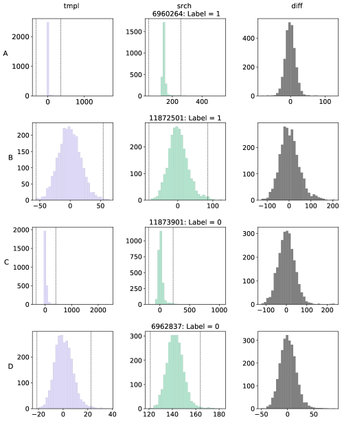
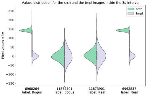
A word about data preparation and normalization is in order as astrophysical images are inherently very different from the images upon which CNNs have been built. When training CNN models for image analysis, each image is typically simply scaled to a common range ( $0-1$ ). However, the dynamic range of an astrophysical image is typically large and the distribution of pixel values is generally very different from Gaussian, with the majority of pixels sitting at low values (the sky) and a few pixels at or near saturation (which in some cases may carry the majority of the information content). Furthermore, in the DIA-set case, the pixel-value distribution of the diff differs qualitatively from the tmpl and srch ones. While the tmpl and srch are typically naturally positive valued with a long tail at the bright end (right-skewed because of the presence of bright astrophysical sources such as galaxies that host transients or stars that vary), the diff image is, in absence of variable or transient sources, symmetric around 0 (see Figure 2).

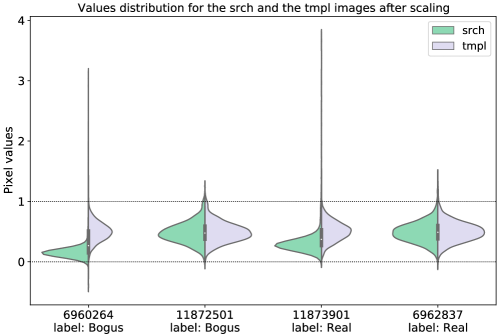
The diff images were standardized to have a mean $\mu=0$ and a standard deviation $\sigma=1$ . The srch and tmpl images, instead, were scaled to map the $\mu\pm 3\sigma$ interval of the original image to $0-1$ . This scheme allows us to retain resolution in the shape of the core of the distribution while also retaining extreme pixel values. Figure 2 shows the distribution of pixel values for four DIA sets, for the same data as in Figure 1, which include two “real” and two “bogus” labels. The distribution moments used for standardization are shown. Appendix A shows the pixel distributions before and after scaling for the same data in some more detail.

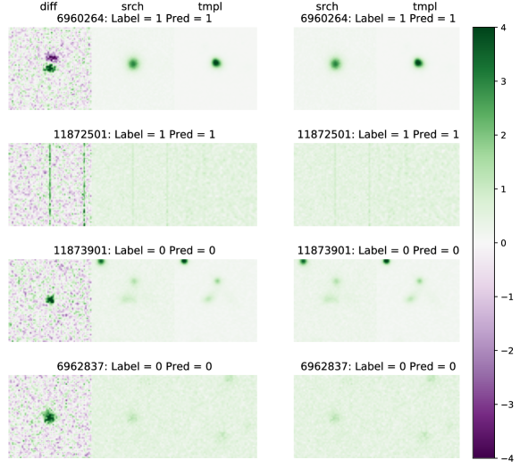
One further decision has to be made in combining the three images in the DIA set to feed them to the CNN. While commonly the images would be stacked depth-wise, we stacked the scaled diff, srch and tmpl horizontally. Thus the size of the data in input to our CNN is ( $N_{tr}\times 51\times 153$ ), where $N_{tr}$ is the number of transients to be considered. Four examples of the data “triplets” in input to our DIA-based CNN are in the left panel of Figure 3. Following this horizontal structure, we mimic closely the way that human scanned this type of data for classification, and we will take advantage of this scheme when examining the models’ decisions in subsection 4.4. We inspected the impact of this choice by comparing the accuracy of a model that was given the images stacked in depth ( $51\times 51\times 3$ ) with the model with $51\times 153$ images in input, with otherwise identical architecture after the first hidden layer, and found that our choice does not affect the overall performance (both models achieved 96% accuracy as will be discussed in section 5; see also Appendix A, Figure 14).

Since our goal is to measure the impact of reducing the information passed to the model the input by not using the DIA, for our noDIA-based models the training and testing data set were constructed in the same way as the previous triplets with the tmpl and srch side-by-side, but without the diff image. Some examples are in the right panel of Figure 3.

4 Methodology

4.1 Basics of Neural Networks

Neural Networks are models that learn important features and feature associations directly from data. They can be used as supervised learning models for classification or regression. They consist of a series of layers of linear combinations of the input data each with real value parameters known as weights and biases, combined with activation functions that enable learning non-linear, potentially very complex, relationships in the data. The weights tell us the relevance of the input feature with respect to the output, and the biases are the offset value that determine the output. Fitting these quantities to the data minimizes the loss, meaning the prediction is as close as possible to the original target/label (Nielsen, 2015). For Deep Neural Networks (DNNs), “deep” refers to the fact that there are multiple hidden layers, between the input and output layer. With this architecture the features learned by each layer do not follow a human selection, rather, the features arise in the analysis of the data (LeCun et al., 2015). Among DNNs, CNN models have layers that represent convolutional filters. More information on DNNs and CNNs can be found in Agarap (2018); Krizhevsky et al. (2012); Dieleman et al. (2015), as well as Gieseke et al. (2017), among many others.

We used the Keras⁷⁷7https://keras.io/api/layers/convolution_layers/convolution2d/. implementation of the CNN (Chollet et al., 2015).

4.2 DIA and noDIA based models architecture

The input of our Neural Networks are the horizontally stacked images of size $51\times 153$ for the DIA-based model (diff, srch, tmpl), and $51\times 102$ for noDIA-based model (srch, tmpl). For both the DIA-based and the noDIA-based, $100,000$ images were used to build the model: $80,000$ images for training and $20,000$ for validation. An additional set of $20,000$ images is used for testing, i.e. the predictions on this test are only done after the model hyperparameters are set, and the result reported throughout are based on this set. The images were selected randomly from the $898,963$ and while certainly training with a larger set can lead to higher accuracy, the amount of images was sufficient for this comparison of DIA-based and noDIA-based models while being conservative with limited computational resource. The data is composed of $50,183$ images labeled as “bogus” and $49,817$ labeled as “real”.

The network architectures used for this work are shown in Figure 4, left panel, for the DIA-based model, and right panel for the noDIA-based model. More details about the architecture can be found in Appendix B. Both architectures follow a similar structure.

In designing the neural networks, we started with the DIA-based model and developed an architecture that would match the performance of Goldstein et al. (2015). While examples exist in the literature of RB models with higher measured performance (see section 2 and Gieseke et al. 2017, Cabrera-Vives et al. 2016, Cabrera-Vives et al. 2017, Liu et al. 2019, Duev et al. 2019, etc.), we emphasize that each one of these models is applied to a different datasets, such that their performance cannot be treated as a benchmark. Furthermore, our goal here is not to replace the DES RB model with a higher performing one, but to measure the impact of the loss of information content in the input caused by removing the diff. Matching the performance of the accepted model for RB separation within the DES is a sufficient result for our purpose. In fact, more complex architectures have been implemented on these data without a significant performance improvement (see Appendix B.2). This leads us to believe that at least a fraction of the 3% incorrect predictions are associated with noisy and incorrect labels (see subsection 4.3).

With this model in hand, we created a noDIA-based with a similar structure in order to enable direct comparison and measure the effect of the change in the input data.

In the development of our models we followed two general guidelines:

1.

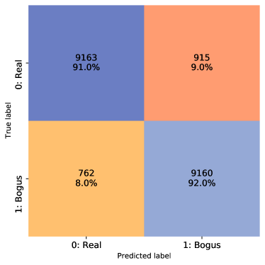
When designing the models, our goal was to push the accuracy of the DIA-based CNN model to match the accuracy of autoscan. While a more exhaustive architectural exploration or a hyperparameter grid search may well lead to increased efficacy, matching the accuracy of autoscan (at $\sim$ 97%) is sufficient for our demonstration. The final architecture used is one that reached the same accuracy as Goldstein et al. (2015), and False Positive and False Negative Rates most similar to the ones obtained in Goldstein et al. (2015) (see Figure 5 and section 5). Once we matched the autoscan performance, we focused on the potential for removing the diff image from the input.
2.

While the architecture of the DIA-based CNN was designed with the attempt to achieve a specific target performance, the architecture of noDIA-based is deliberately kept as close as possible to that of the DIA-based model. This enables a direct comparison of the effects of the removal of the diff image. The architecture of noDIA-based, shown on the right in Figure 4 was not optimized explicitly for RB classification, rather was inherited from the DIA-based model, only modifying the original design to adapt for the different dimensionality of the input data. One further deliberate modification is implemented in the choice of a single-filter first layer for noDIA-based. The diff image is produced by matching the PSF of the science image in the template (and scaling the brightness with a trivial scaling factor). Everything else needed for the RB classification is contained in the tmpl-srch pair as is in the tmpl-srch-diff triplet. Thus the CNN that is not offered the diff image needs to learn the image PSF, which is constant across the postage stamp size image and it should be possible to model it with a single filter.

4.3 Performance assessment

Although our goal was to measure the performance impact of the loss of input, as part of our performance assessment tasks, we conducted an extensive hyperparameter search on the existing noDIA-based architecture and tested alternative pre-packaged architectures for the DIA-based known to perform well on image classification.

We performed a grid searches varying the kernel size of the convolutional layers and the batch size (see Appendix B.2, Table 10). The optimal parameters are reported for each model in Appendix B. We re-trained two pre-made deep learning models, VGG16 (Simonyan & Zisserman, 2014) and ResNet 50-V2 (He et al., 2016), (see Appendix B.1, Table 5) with the same data used to train the DIA-based presented here. Neither outperformed our DIA-based model, while both presented issues with overfitting. Pre-made architectures force constraints on the size of the images used to train the model, thus these models were trained with input images stacked in depth ( $51\times 51\times 3$ , see subsection 3.1). The small size of our postage stamps also limits the available architectures to models with relatively few layers (due to the repeated application of pooling layers). VGG16 achieves a performance similar to our model’s in terms of the testing accuracy with 0.9603, but trains faster and begins overfitting after $\sim 20$ epochs ( where overfitting is diagnosed visually from the loss curves identifying the epoch at which the validation loss starts increasing in spite of continued improvements in the training loss). ResNet 50-V2 shows signs of overfitting throughout the entire training process and only achieves a test accuracy of 0.9416. We conclude that this historical data set contains some level of label inaccuracy such that surpassing the performance of autoscan may be effectively impossible.

We remind the reader that in this dataset, simulated supernovae are by default labeled as Real. However, we found that many images labeled as Bogus, upon visual inspection could be re-classified as transients (we estimate between 3% and 10% of the Bogus labels could be reclassified (see Appendix D). This dataset has now been archived and cannot be further validated by, for example, assessing the recurrence of transients at a sky position to validate the bogus nature of a non-simulated detection. Thus, while CNN models do exist in the literature with higher accuracy, our model’s performance is considered optimal at $0.961$ . We performed a $k$ -fold cross-validation with $k=6$ for the noDIA-based model. The average accuracy for the test data set is $0.911\pm 0.005$ .

4.4 Saliency maps

Saliency maps quantify the importance of each pixel of an image in input to a CNN in the training process. They provide some level of interpretability through a process akin to feature importance analysis by enabling an assessment of which pixels the model relies on the most for the final classification. If the task were, for example, to identify cats and dogs in images, the expectation will be to find that the most important pixels are located within the dog or cat bodies, and not in the surrounding, while if the task were to identify activities performed by cats and dogs, one may find the important pixels both within the dogs and in the surrounding, particularly in objects associated with the performed tasks. Furthermore, some portions of the subject’s body may be most distinctive (ears, nose) and we would expect more importance given to those pixels. The “importance”: of a pixel would be simply measured by the weight the trained NN assigns to that pixel in the case of a single-layer perceptron, but in the case of Deep Neural Networks, a highly non-linear operation is performed on the input data, and the importance, or saliency, of an input feature, or pixel, is harder to assess. Saliency maps have been extracted from CNNs and studied in earlier works, chiefly in Lee et al. (2016). Subsequently, saliency maps have been used as a tool for improving the efficiency of the performance of the CNNs (see for example Lee et al. 2021). Within the field of transient detection, Reyes et al. (2018), have leveraged saliency maps to identify the most relevant pixels and improve performance on transient classification. We go one step further and use the saliency maps to investigate how the model leverages the DIA image and what information the model uses in its absence.

We follow Simonyan et al. (2014)’s definition of saliency: denoting the class score with $S_{c}$ , such that the NN output on image $\mathcal{I}$ is represented by $S_{c}(\mathcal{I})$ , the saliency map is given by :

	$\displaystyle S_{c}(\mathcal{I})\approx w^{T}\mathcal{I}+b,$		(2)
	$\displaystyle w=\frac{\partial S_{c}}{\partial\mathcal{I}}\biggr{\rvert}_{\mathcal{I}_{0}}.$		(3)

That is: $w^{T}$ is the weight and $b$ the bias of the model. $w$ is the derivative of $S_{c}$ with respect to $\mathcal{I}$ calculated specifically in the local neighborhood of pixel $\mathcal{I}_{0}$ , and the approximation sign indicates a first order Taylor expansion has been used to approximate the solution. Each pixel in an image in the training set is associated with the corresponding pixel in the saliency map, and the saliency score (the importance) of that pixel measures the change in model output as a function of changes in the value of that input pixel by back-propagation. The higher the value of a pixel in a saliency map, the more influence that pixel has in the final classification. In this work we also refer to these maps as maps of pixel importance.

In our case, given the side-by-side organization of the three elements of the input image set, the saliency maps can help us assess how much the DIA-based model relied on the diff to enable correct classification, and, thus, provide some intuition in the difficulty of the challenge offered to the noDIA-based model.

For the DIA-based model we have an expectation guided by intuition: that a greater concentration of important pixels should be found in the diff image. In section 5, we will consider the veracity of this hypothesis both qualitatively by visually inspecting the saliency maps, and by designing a saliency-based metric that enables a quantitative approach. We calculated the normalized sum of the saliency pixel values for each third of the image-triplet, corresponding to diff, srch, tmpl. Indicating with $I$ the importance of the segment of an image, ( $I_{\mathrm{diff}},I_{\mathrm{srch}},I_{\mathrm{tmpl}}$ ), with $p$ a pixel and $s_{p}$ its corresponding saliency value, and utilizing the subscript $d$ , $s$ and $t$ , to refer to pixels respectively in the diff, srch and tmpl, we have:

\displaystyle\begin{split}I_{\mathrm{diff}}=\frac{\sum_{p_{d}}{s_{p_{d}}}}{\sum_{p}{s_{p}}};\\ I_{\mathrm{srch}}=\frac{\sum_{p_{s}}{s_{p_{s}}}}{\sum_{p}{s_{p}}};\\ I_{\mathrm{tmpl}}=\frac{\sum_{p_{t}}{s_{p_{t}}}}{\sum_{p}{s_{p}}}.\end{split}

(4)

The numerators capture the importance of each third of an image while the denominator normalizes each metric by the total sum of the saliency pixel values, so that $I_{\mathrm{diff}}+I_{\mathrm{srch}}+I_{\mathrm{tmpl}}=1$ .

This metric allows us to assess the relative importance of the diff (srch or tmpl) component of the image in performing RB classification. Results from these metrics are discussed in detail in subsection 5.1.

5 Results

The accuracies of our models and their respective errors, calculated as the standard deviation, are presented in Table 1. The DIA-based model reached, by design, the accuracy of our benchmark model autoscan: 97% on True Negative (TN) rate and 95% on True Positive (TP) rate (see section 4). We remind the reader that we use the autoscan convention for the definition of TN and TP: Positive is a “real” transient (label = 0), negative is a “bogus” (label = 1). There is a drop of $\sim 4\%$ between the accuracy of the DIA-based and the noDIA-based models. Along with the accuracy, in Table 1 we present computational costs of training on 20,000 images measured in CPU Node hours,⁸⁸8The computational cost was calculated by using the formula given in https://docs.nersc.gov/jobs/policy/ and the allocations information given by the system Iris https://iris.nersc.gov. Training time is reported in CPU hours. Prediction time is reported per “postage stamp” (1ms) and the classification operation is trivially parallelizable (can be run independently on each postage stamp). and the clock time for the prediction for one single image.

DIA-based	0.965	$0.004$	0.960	$\sim$ 35	$1.00\pm 0.03$
Model	Accuracy			Training⁸	Prediction⁸
Model	Train	Test	Val	CPU	Clock-time
				(hours)	(ms)
DIA-based	0.965	$0.961\pm$	0.960	$\sim$ 35	$1.00\pm 0.03$
noDIA-based	0.920	$0.911\pm$	0.914	$\sim$ 56	$0.30\pm 0.01$
noDIA-based	0.920	$0.005$	0.914	$\sim$ 56	$0.30\pm 0.01$

Table 1: Comparative table of the accuracy and computational cost for training, testing and validation data for the DIA-based (Figure 4, left) and noDIA-based (Figure 4, right) models.

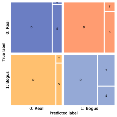
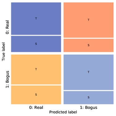
Confusion matrices for the testing set are shown for the DIA-based model in left panel of Figure 5 and for the noDIA-based model in the right panel of the same figure. In this figure, as in the following confusion matrices and histograms that we will present in subsection 5.1, correct predictions are indicated in shades of blue, incorrect in shades of orange, and darker shades are associated with the true labels. The percent accuracy for each class, True Positives (TP), True Negatives (TN), False Positives (FP), and False Negatives (FN), as well as the number of images in each class are reported within the figure.

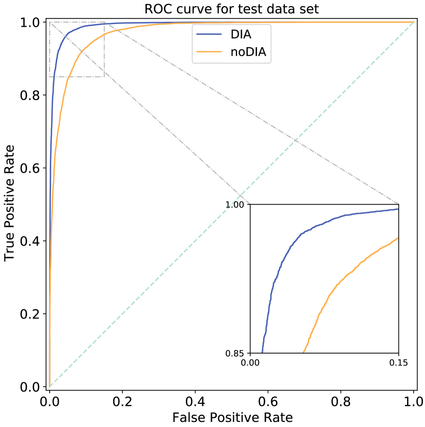
The Receiver Operating Characteristic (ROC) curve shows the relation between the True Positive Rate (TP / (TP + FN)) also know as recall, and the False Positive Rate (FP / (FP + TN)) when changing the threshold value (e.g., a threshold of 0.5 will indicated that values greater than 0.5 would be classified as “bogus”). The ROC for the testing data for the DIA-based and noDIA-based models are presented in Figure 6. The Area Under the Curve (AUC), which can be used as a comprehensive metric of the aggregated classification performance of a model (Hanley & McNeil, 1983; Hernández-Orallo et al., 2012), is 0.992 and 0.973 for the DIA-based and noDIA-based models respectively.

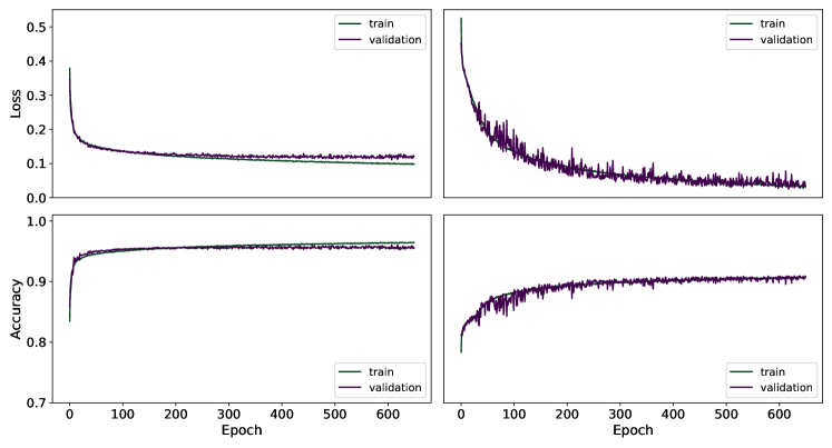
The loss and the accuracy curves in the left panel of Figure 7 for the DIA-based model shows some evidence of overfitting (the validation curve flattens compared to the training curve) starting just a few epochs before training came to end of the 350-epochs; meanwhile, for the noDIA-based model in right Figure 7, after $650$ epochs there was no visual evidence of overfitting indicating that the model is still learning generalized information from the data; yet the accuracy improvements from epoch $350$ to $650$ were small.

The nature of the noDIA-based model leads to hypothesize that because the input data contains less information, this model takes longer to learn features from the data to be able to classify them. The noDIA-based model took in fact longer (more epochs) to come to stable accuracy and loss values. The loss and accuracy curves are also noisier for the validation of the noDIA-based model in right Figure 7 compared to the DIA-based model. This also can be explained with the same argument: the noDIA-based model had a harder problem to solve and this is reflected in a noisier path to minimization. We conclude that this $\sim$ 4% loss in accuracy is directly related to the loss of information in the input caused by dropping the diff in input. In addition, we tested if longer training or slightly richer architectures could make up for the loss of diff and found that neither extending the training beyond 650 epochs or adding convolutional layers improved performance (see Appendix B.1, Table 8, Table 9).

5.1 A peek into the model decisions through saliency maps

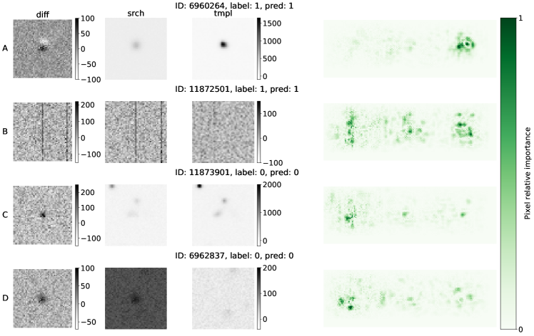
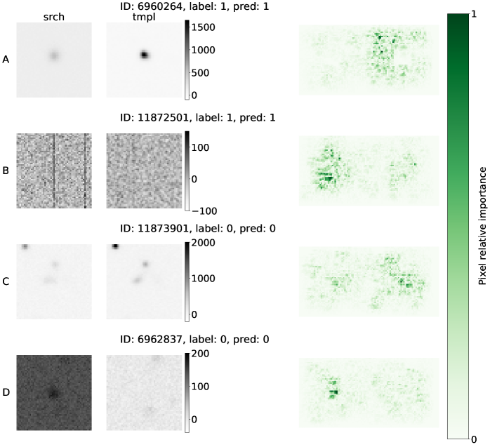
In subsection 3.1, we described how the importance of individual image pixels in the RB prediction performed by our models can be measured, and the design of a saliency-based metric to assess which component of the image is most important to perform the RB classification. Here we inspect the saliency maps, both visually and quantitatively through the measured values of $I_{\mathrm{diff}}$ , $I_{\mathrm{srch}}$ , and $I_{\mathrm{tmpl}}$ .

In Figure 8 and Figure 9 we show the four transients we considered as examples throughout this work, the same images used in Figure 1 and Figure 3, and the corresponding saliency maps for the DIA-based model and noDIA-based model respectively. Figure 10 and Figure 11 report the results of Equation 4 for the objects in our training set.

Lets start with some considerations about the saliency maps for the four image examples for the DIA-based model (Figure 8), and specifically from panels C and D were the transients were correctly predicted as “real”. We observe that the greatest concentration of important pixels for both these images is found in the left-most third of the image: $I_{\mathrm{diff}}\sim 0.5$ for both. We speculate, from our experience in labeling real/bogus by visual inspection and consulting with some of the human scanners that labeled the original autoscan images, that this behaviour is similar to what a human scanner would do: if in the diff image there is a clearly real transient, the scanner would not need to study in detail the srch and tmpl images.

Figure 8A and B show correctly classified “bogus” transients. In Figure 8A, a “bogus” produced likely by a moving object displaying a classical dipole, the majority of the important pixels are located in the tmpl ( $I_{\mathrm{tmpl}}\sim 0.54$ ), concentrated around the location of the central source and the location where its “ghost” image is (the coordinates corresponding to the location the bright patch of pixels in the diff, but in the tmpl portion of the composite image). In Figure 8B, there is no central source and the detection is triggered by an image artifact. The important pixels are found in all three image segments and are spread around a large area of each image: the model has inspected the image in its entirety to decide the classification. Following our considerations about the similarity between the CNN and human decision process, having discussed the typical visual inspection process with members of the DES team that human-labeled this data set, we find that, here too, the CNN mimics closely what a human scanner would do: because there is not a clear central source (a “real” object) in the diff, the scanner wouldn’t simply draw a conclusion based on the diff but instead would analyze the srch and tmpl images to extract more information from the context and enable a robust classification. However, it should be noted that no quantitative studies of the features the human scanners use to classify transients has been done, thus this remains simply an intriguing suggestion.

For the case of the noDIA-based model, the expectation was less clear: both the srch and the tmpl images are necessary to “reconstruct” the information contained in the diff, and while the pixels overlapping with the central transient are obviously expected to be important, the pixels that surround it are necessary to essentially reproduce the scaling and PSF-matching operations between tmpl and srch that the DIA performs. Accordingly, the saliency maps presented in Figure 9 are more difficult to interpret: in all four cases, important pixels are found all over the composite images.

To explore how the choice of important pixels may depend on the image label and on the correct classification we report the fraction of images for which the diff (srch, tmpl) is the dominant source of important pixels within the confusion matrix in Figure 10. To do this, we use a rough but intuitive cutoff: if the normalized sum of the saliency pixels in a third of the image is larger than $\frac{1}{3}$ , then we deduce that the model principally used that component for its decision. For example, where $I_{\mathrm{diff}}>0.33$ , we conclude that the model principally relied on diff to make the RB classification. With this cut-off we can assess if there are differences in the model behavior when classifying objects as a function of their labels or their classification. In all four cases (all combinations of “real” and “bogus” label and prediction) the concentration of important pixels is largest in the portion of the image corresponding to the diff in the DIA-based model. It is however interesting to note that, in order to correctly classify the “bogus”, the DIA-based model uses the template and search image more heavily than in all other cases (diff, srch, tmpl, = 66%, 13%, 21% for TN, while $I_{\it diff}>80\%$ for TP, FP, and FN).

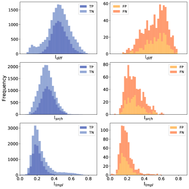
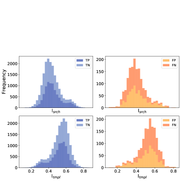
The cut-off method described above does not allow us to distinguish between cases where multiple sections of the images were used jointly, perhaps with similar importance, from cases where the model truly only relied on one section of the image. For that, we take a closer look at the distribution of saliency values. In Figure 11 we show the distribution of values of the three metrics defined in Equation 4 for each of the four cases: TP and TN, in shades of blue, FP and FN, in shades of orange, following the color-scheme adopted in Figure 5 and Figure 10. For the DIA-based model (the two left-most columns), for the majority of the 20,000 images in the training set $I_{\mathrm{diff}}>0.33$ , but there is a secondary pick in the $I_{\mathrm{diff}}$ distribution near $I_{\mathrm{diff}}\sim 0.1$ populated entirely by TN cases, complementary to a long right tail in the $I_{\mathrm{tmpl}}$ distribution ( $I_{\mathrm{tmpl}}>0.4$ ). This confirms that the correct classification in the presence of real transients relies on diff, but tmpl and srch become important to correctly classify bogus transients, just like we had seen in the exemplary cases in Figure 8. We note also that the general shape of each distribution ( $I_{\mathrm{diff}}$ , $I_{\mathrm{srch}}$ , $I_{\mathrm{tmpl}}$ ) is similar for the TP and TN case (blue) and for the FP and FN cases (orange).

For the noDIA-based model the important pixels are concentrated in the tmpl for most images ( $I_{\mathrm{tmpl}}>0.5$ ) for both correct and incorrect classifications. This is somewhat counter-intuitive since the tmpl does not contain the transient itself! However, one may speculate that this is because the tmpl, a higer quality image, contains more accurate information about the context in which the transient arises: e.g., if it is located near a galaxy or not. This information is important to the classification. It is also interesting to note that for the transients predicted as “real” in both TP and FP, the fraction of images that leveraged primarily the tmpl is approximately $2/3$ , and for images predicted as “bogus”, in both TN and FN, it is approximately $3/4$ .

To help guide the interpretation of the saliency maps, a few more maps are plotted in Appendix D. Where we provide 6 examples per each class of the confusion matrix, for both the DIA-based and the noDIA-based models.

5.2 Computational cost of our models

The computational cost of our models, reported in CPU Node hours in Table 1, confirms that while training a CNN model for RB can be computationally expensive, and significantly more so if the diff is not used in input (noDIA-based), the model prediction only takes a few seconds even on large datasets. Using a NN-based platform, the computational costs are front-loaded. In transient detection this could mean that the observation-to-transient discovery process can be rapid, while computation time can be spent during off-sky hours (principally to build templates). Furthermore, while the training time is longer for the noDIA-based model than for the model that uses the diff in input (DIA-based) the computational cost of the forward-pass (prediction) scales superlinearly with the size of the feature set (pixels), so that our noDIA-based model takes less than half the time than the DIA-based one to perform the RB task. With a clock time of 0.3 ms per 51 $\times$ 51 pixels postage stamp, predicting over the full DES focal plane would take $\sim 1$ minute. However, we note that at this stage of our work we still rely on the DIA in several ways: while the tmpl and srch in input to noDIA-based are not PSF matched, this proof of concept is performed on transients that were detected in diff images, and we leverage the alignment of tmpl and srch and centering of the postage stamp that arose from the DIA (see section 6). Conversely, predictions would only need to be done in correspondence of the sources detected in the tmpl and srch images, and not for the entire CCD plane.

6 Future work and limitation of this work

This work is targeted to the investigation of CNN RB model performance, with and without diff in input, on a single data set, the same dataset upon which the development of the random-forest-based autoscan was based (see section 3). This approach enables a straightforward comparison, but it comports some limitations.

The labels in our data set come from simulations of SNe (label = 0) and visual inspection that classifies artifacts and moving objects (label = 1). We reserve to future work the investigation of the efficacy of the model on transients of different nature, including quasars (QSOs), strong lensed systems, Tidal Disruption Events (TDEs), and supernovae of different types. These transients may have characteristically different associations with the host galaxy, including preferences for different galaxy types and locations with respect to the galaxy center, compared to the simulated SNe events in our training set.

Specifically thinking of Rubin LSST data, an additional source of variability may be introduced by Differential Chromatic Refraction effects (Abbott et al., 2018; Richards et al., 2018), or stars with significant proper motion which, due to exquisite image quality of the Rubin images, would be detectable effects.

While we demonstrated CNN model’s potential in the detection of transients without DIA, we did not address the question of completeness as a function of srch or tmpl depth or the potential for performing accurate photometry without DIA.

We trained multiple network architectures to attempt to improve our prediction performance, as discussed in section 4. None of the models we trained achieved an accuracy that significantly outperformed the random forest-based autoscan, and none of the noDIA-based versions of our models compensated for the $\sim 4\%$ loss induced by the removal of the diff in input. Our efforts included training the original noDIA-based for many more epochs, tuning hyperparameters, adding convolutional layers, and adding layers after the last convolutional layer but before the flatten layers to reduce bottlenecks. We intend to continue investigating alternative architectures in future work.

Finally, we note that our models did in fact implicitly leverage some of the information generated by the DIA even when they did not use the diff image itself as input. First, the tmpl and srch images are de-warped. Since the transient alerts are generated from aligned DIA images, the transient source is always located at the image center in our data. We use postage stamps that were, however, not PSF matched or scaled to match the template brightness. To move beyond a proof-of-concept, in future work we will re-train and apply our models to images whose alignment does not depend on the existence of a transient.

7 Conclusions

In this work, we have measured the accuracy loss associated with the removal of the diff image in input to a CNN trained in classifying true astrophysical transients from artifacts and moving objects (a task generally known as “real-bogus”). We have demonstrated that, while a model with $\sim 91.1\%$ accuracy can be built without leveraging the results of a difference image analysis (DIA) pipeline that constructs a “template-subtracted” image, there is a loss of performance of a few percentage points.

Starting from the Dark Energy Survey dataset that supported the creation of the well known real-bogus autoscan model (Goldstein et al., 2015), we first built a CNN-based model, dubbed DIA-based, that uses a sky template (tmpl), a nightly image (srch), and a template-subtracted version of the nightly image (diff) that performs real-bogus classification at the level of autoscan model. Our DIA-based model reaches a $97\%$ accuracy in the bogus classification with an Area-Under-the-Curve of 0.992 and does not require human decision in the feature engineering or extraction phase.

We then created noDIA-based, a model which uses only the tmpl and srch images and can extract information that enables the identification of bogus transients with $91.1\%$ accuracy. We attribute this performance decrease directly to the loss of information about the PSF of the original image since, in addition to what is contained in the tmpl and srch pair, the diff contains information about the PSF used to degrade the tmpl to match the quality of the srch image (section 2). Thus, the convolutional architecture has been unable to recover that information.

We further investigated what information enables the real-bogus classification in both the DIA-based and noDIA-based models and demonstrated that a CNN trained with the DIA output primarily uses the information in the diff image to make the final classification, and that the model examines a diff-srch-tmpl image-set fundamentally differently in the cases where there is a transient, than in the cases where there is not one. The noDIA-based model, conversely, takes a more comprehensive look at both tmpl and srch images, but relies primarily on tmpl to enable the reconstruction of the information found in the diff.

Implementation of this methodology in future surveys could reduce the time and computational cost required for classifying transients by entirely omitting the construction of the difference images.

8 Acknowledgment

TAC and FBB acknowledge the support of the LSST Corporation and the Enabling Science Grant program that partially supported TAC through Grant No. 2021-040, Universidad Nacional de Colombia and University of Delaware for the Beyond Research Program (2020) and Summer Research Exchange (2021). MS and HQ were supported by DOE grant DE-FOA-0002424 and NSF grant AST-2108094.

TAC: Prepared the data, conducted the analysis, created and maintains the machine learning models, wrote the manuscript. FBB: Advised on data selection, curation, and preparation, selection and design, revised the manuscript. GD: Advised on data preparation and model selection and design, revised the manuscript. MS: Advised on data selection, shared knowledge about the compilation and curation of the original dataset, revised the manuscript. HQ: Advised on data preparation and model design, revised the manuscript.

This paper has undergone internal review in the LSST Dark Energy Science Collaboration. The internal reviewers were: Viviana Acquaviva, Suhail Dhawan, and Michael Wood-Vasey.

The DESC acknowledges ongoing support from the Institut National de Physique Nucléaire et de Physique des Particules in France; the Science & Technology Facilities Council in the United Kingdom; and the Department of Energy, the National Science Foundation, and the LSST Corporation in the United States. DESC uses resources of the IN2P3 Computing Center (CC-IN2P3–Lyon/Villeurbanne - France) funded by the Centre National de la Recherche Scientifique; the National Energy Research Scientific Computing Center, a DOE Office of Science User Facility supported by the Office of Science of the U.S. Department of Energy under Contract No. DE-AC02-05CH11231; STFC DiRAC HPC Facilities, funded by UK BIS National E-infrastructure capital grants; and the UK particle physics grid, supported by the GridPP Collaboration. This work was performed in part under DOE Contract DE-AC02-76SF00515.

This project used public archival data from the Dark Energy Survey (DES). Funding for the DES Projects has been provided by the U.S. Department of Energy, the U.S. National Science Foundation, the Ministry of Science and Education of Spain, the Science and Technology Facilities Council of the United Kingdom, the Higher Education Funding Council for England, the National Center for Supercomputing Applications at the University of Illinois at Urbana–Champaign, the Kavli Institute of Cosmological Physics at the University of Chicago, the Center for Cosmology and Astro-Particle Physics at the Ohio State University, the Mitchell Institute for Fundamental Physics and Astronomy at Texas A&M University, Financiadora de Estudos e Projetos, Fundação Carlos Chagas Filho de Amparo à Pesquisa do Estado do Rio de Janeiro, Conselho Nacional de Desenvolvimento Científico e Tecnológico and the Ministério da Ciência, Tecnologia e Inovação, the Deutsche Forschungsgemeinschaft and the Collaborating Institutions in the Dark Energy Survey. The Collaborating Institutions are Argonne National Laboratory, the University of California at Santa Cruz, the University of Cambridge, Centro de Investigaciones Enérgeticas, Medioambientales y Tecnológicas–Madrid, the University of Chicago, University College London, the DES-Brazil Consortium, the University of Edinburgh, the Eidgenössische Technische Hochschule (ETH) Zürich, Fermi National Accelerator Laboratory, the University of Illinois at Urbana-Champaign, the Institut de Ciències de l’Espai (IEEC/CSIC), the Institut de Física d’Altes Energies, Lawrence Berkeley National Laboratory, the Ludwig-Maximilians Universität München and the associated Excellence Cluster Universe, the University of Michigan, the National Optical Astronomy Observatory, the University of Nottingham, The Ohio State University, the OzDES Membership Consortium, the University of Pennsylvania, the University of Portsmouth, SLAC National Accelerator Laboratory, Stanford University, the University of Sussex, and Texas A&M University.

Based in part on observations at Cerro Tololo Inter-American Observatory, National Optical Astronomy Observatory, which is operated by the Association of Universities for Research in Astronomy (AURA) under a cooperative agreement with the National Science Foundation.

This research used resources of the National Energy Research Scientific Computing Center (NERSC), a U.S. Department of Energy Office of Science User Facility located at Lawrence Berkeley National Laboratory, operated under Contract No. DE-AC02-05CH1123.

This research was supported in part through the use of DARWIN computing system: DARWIN – A Resource for Computational and Data-intensive Research at the University of Delaware and in the Delaware Region, which is supported by NSF under Grant Number: 1919839, Rudolf Eigenmann, Benjamin E. Bagozzi, Arthi Jayaraman, William Totten, and Cathy H. Wu, University of Delaware, 2021.

This material is based upon work supported by the University of Delaware Graduate College through the Unidel Distinguished Graduate Scholar Award. Any opinions, findings, and conclusions or recommendations expressed in this material are those of the author(s).

TAC thanks the LSSTC Data Science Fellowship Program, which is funded by LSSTC, NSF Cybertraining Grant #1829740, the Brinson Foundation, and the Moore Foundation; her participation in the program has benefited this work.

All of our code is written in Python using the following packages:

•

TensorFlow (Abadi et al., 2015)
•

Keras (Chollet et al., 2015)
•

numpy (Harris et al., 2020)
•

astropy (Astropy Collaboration et al., 2013, 2018)
•

pandas (Wes McKinney, 2010; pandas development team, 2020)
•

matplotlib (Hunter, 2007)
•

seaborn (Waskom, 2021)

9 Data availability

The data underlying this article are available in https://portal.nersc.gov/project/dessn/autoscan/#tdata, and explain in more detail in Goldstein et al. (2015).

References

Abadi et al. (2015) Abadi, M., Agarwal, A., Barham, P., et al. 2015, TensorFlow: Large-Scale Machine Learning on Heterogeneous Systems. https://www.tensorflow.org/
Abbott et al. (2018) Abbott, T. M. C., Abdalla, F. B., Allam, S., et al. 2018, The Astrophysical Journal Supplement Series, 239, 18, doi: 10.3847/1538-4365/aae9f0
Agarap (2018) Agarap, A. F. 2018, CoRR, abs/1803.08375. https://arxiv.org/abs/1803.08375
Alard & Lupton (1998) Alard, C., & Lupton, R. H. 1998, The Astrophysical Journal, 503, 325, doi: 10.1086/305984
Astropy Collaboration et al. (2013) Astropy Collaboration, Robitaille, T. P., Tollerud, E. J., et al. 2013, A&A, 558, A33, doi: 10.1051/0004-6361/201322068
Astropy Collaboration et al. (2018) Astropy Collaboration, Price-Whelan, A. M., Sipőcz, B. M., et al. 2018, AJ, 156, 123, doi: 10.3847/1538-3881/aabc4f
Bellm et al. (2018) Bellm, E. C., Kulkarni, S. R., Graham, M. J., et al. 2018, Publications of the Astronomical Society of the Pacific, 131, 018002, doi: 10.1088/1538-3873/aaecbe
Bloom et al. (2012) Bloom, J., Richards, J., Nugent, P., et al. 2012, Publications of the Astronomical Society of the Pacific, 124, 1175
Cabrera-Vives et al. (2017) Cabrera-Vives, G., Reyes, I., Förster, F., Estévez, P. A., & Maureira, J.-C. 2017, The Astrophysical Journal, 836, 97, doi: 10.3847/1538-4357/836/1/97
Cabrera-Vives et al. (2016) Cabrera-Vives, G., Reyes, I., Förster, F., Estévez, P. A., & Maureira, J.-C. 2016, in 2016 International Joint Conference on Neural Networks (IJCNN), 251–258, doi: 10.1109/IJCNN.2016.7727206
Carrasco-Davis et al. (2019) Carrasco-Davis, R., Cabrera-Vives, G., Förster, F., et al. 2019, Publications of the Astronomical Society of the Pacific, 131, 108006, doi: 10.1088/1538-3873/aaef12
Carrasco-Davis et al. (2021) Carrasco-Davis, R., Reyes, E., Valenzuela, C., et al. 2021, Alert Classification for the ALeRCE Broker System: The Real-time Stamp Classifier. https://arxiv.org/abs/2008.03309
Chollet et al. (2015) Chollet, F., et al. 2015, Keras, GitHub. https://github.com/fchollet/keras
Crotts (1992) Crotts, A. P. S. 1992, ApJ, 399, L43, doi: 10.1086/186602
Deng et al. (2009) Deng, J., Dong, W., Socher, R., et al. 2009, in 2009 IEEE Conference on Computer Vision and Pattern Recognition, 248–255, doi: 10.1109/CVPR.2009.5206848
Dieleman et al. (2015) Dieleman, S., Willett, K. W., & Dambre, J. 2015, Monthly Notices of the Royal Astronomical Society, 450, 1441–1459, doi: 10.1093/mnras/stv632
Drake et al. (2009) Drake, A. J., Djorgovski, S. G., Mahabal, A., et al. 2009, The Astrophysical Journal, 696, 870, doi: 10.1088/0004-637x/696/1/870
Duev et al. (2019) Duev, D. A., Mahabal, A., Masci, F. J., et al. 2019, Monthly Notices of the Royal Astronomical Society, 489, 3582, doi: 10.1093/mnras/stz2357
Förster et al. (2016) Förster, F., Maureira, J. C., Martí n, J. S., et al. 2016, The Astrophysical Journal, 832, 155, doi: 10.3847/0004-637x/832/2/155
Gabbard et al. (2018) Gabbard, H., Williams, M., Hayes, F., & Messenger, C. 2018, Phys. Rev. Lett., 120, 141103, doi: 10.1103/PhysRevLett.120.141103
Gieseke et al. (2017) Gieseke, F., Bloemen, S., van den Bogaard, C., et al. 2017, Monthly Notices of the Royal Astronomical Society, 472, 3101–3114, doi: 10.1093/mnras/stx2161
Goldstein et al. (2015) Goldstein, D. A., D’Andrea, C. B., Fischer, J. A., et al. 2015, The Astronomical Journal, 150, 82, doi: 10.1088/0004-6256/150/3/82
Gunn et al. (2006) Gunn, J. E., Siegmund, W. A., Mannery, E. J., et al. 2006, The Astronomical Journal, 131, 2332–2359, doi: 10.1086/500975
Hambleton et al. (2020) Hambleton, K., Bianco, F., Clementini, G., et al. 2020, Research Notes of the AAS, 4, 40, doi: 10.3847/2515-5172/ab8129
Hanley & McNeil (1983) Hanley, J. A., & McNeil, B. J. 1983, Radiology, 148, 839
Harris et al. (2020) Harris, C. R., Millman, K. J., van der Walt, S. J., et al. 2020, Nature, 585, 357, doi: 10.1038/s41586-020-2649-2
Harvey et al. (2013) Harvey, D., C. Lintott, T. K., Marshall, P., Willett, K., & Zoo, G. 2013, Galaxy Zoo - The Galaxy Challenge, Kaggle. https://kaggle.com/competitions/galaxy-zoo-the-galaxy-challenge
He et al. (2016) He, K., Zhang, X., Ren, S., & Sun, J. 2016, Identity Mappings in Deep Residual Networks, arXiv, doi: 10.48550/ARXIV.1603.05027
Hernández-Orallo et al. (2012) Hernández-Orallo, J., Flach, P., & Ferri Ramírez, C. 2012, Journal of Machine Learning Research, 13, 2813
Ho (1995) Ho, T. K. 1995, in Proceedings of 3rd international conference on document analysis and recognition, Vol. 1, IEEE, 278–282
Hunter (2007) Hunter, J. D. 2007, Computing in Science & Engineering, 9, 90, doi: 10.1109/MCSE.2007.55
Ivezić et al. (2019) Ivezić, Ž., Kahn, S. M., Tyson, J. A., et al. 2019, ApJ, 873, 111, doi: 10.3847/1538-4357/ab042c
Ivezić et al. (2019) Ivezić, Ž., Kahn, S. M., Tyson, J. A., et al. 2019, The Astrophysical Journal, 873, 111
Kessler et al. (2015) Kessler, R., Marriner, J., Childress, M., et al. 2015, The Astronomical Journal, 150, 172, doi: 10.1088/0004-6256/150/6/172
Kim & Brunner (2016) Kim, E. J., & Brunner, R. J. 2016, Monthly Notices of the Royal Astronomical Society, 464, 4463–4475, doi: 10.1093/mnras/stw2672
Krizhevsky et al. (2012) Krizhevsky, A., Sutskever, I., & Hinton, G. E. 2012, in Proceedings of the 25th International Conference on Neural Information Processing Systems - Volume 1, NIPS’12 (Red Hook, NY, USA: Curran Associates Inc.), 1097–1105
LeCun et al. (2015) LeCun, Y., Bengio, Y., & Hinton, G. 2015, Nature, 521, 436–444, doi: 10.1038/nature14539
LeCun et al. (1989) LeCun, Y., et al. 1989, Connectionism in perspective, 19, 143
Lee et al. (2016) Lee, G., Tai, Y.-W., & Kim, J. 2016, in Proceedings of the IEEE Conference on Computer Vision and Pattern Recognition (CVPR)
Lee et al. (2021) Lee, K. H., Park, C., Oh, J., & Kwak, N. 2021, CoRR, abs/2105.00937
LeNail (2019) LeNail, A. 2019, Journal of Open Source Software, 4, 747, doi: 10.21105/joss.00747
Liu et al. (2019) Liu, W., Zhu, M., Dai, C., et al. 2019, Research in Astronomy and Astrophysics, 19, 042, doi: 10.1088/1674-4527/19/3/42
Mahabal et al. (2019) Mahabal, A., Rebbapragada, U., Walters, R., et al. 2019, PASP, 131, 038002, doi: 10.1088/1538-3873/aaf3fa
Mong et al. (2020) Mong, Y.-L., Ackley, K., Galloway, D. K., et al. 2020, Monthly Notices of the Royal Astronomical Society, 499, 6009–6017, doi: 10.1093/mnras/staa3096
Nielsen (2015) Nielsen, M. A. 2015, Neural Network and Deep Learning (Determination Press)
pandas development team (2020) pandas development team, T. 2020, pandas-dev/pandas: Pandas, latest, Zenodo, doi: 10.5281/zenodo.3509134
Reyes et al. (2018) Reyes, E., Estevez, P. A., Reyes, I., et al. 2018, in 2018 International Joint Conference on Neural Networks (IJCNN) (IEEE), doi: 10.1109/ijcnn.2018.8489627
Richards et al. (2018) Richards, G., Peters, C., Martin, B., & Bauer, F. E. 2018
Sedaghat & Mahabal (2018) Sedaghat, N., & Mahabal, A. 2018, Monthly Notices of the Royal Astronomical Society, 476, 5365, doi: 10.1093/mnras/sty613
Simonyan et al. (2014) Simonyan, K., Vedaldi, A., & Zisserman, A. 2014, Deep Inside Convolutional Networks: Visualising Image Classification Models and Saliency Maps. https://arxiv.org/abs/1312.6034
Simonyan & Zisserman (2014) Simonyan, K., & Zisserman, A. 2014, Very Deep Convolutional Networks for Large-Scale Image Recognition, arXiv, doi: 10.48550/ARXIV.1409.1556
Sánchez et al. (2019) Sánchez, B., Domínguez R., M., Lares, M., et al. 2019, Astronomy and Computing, 28, 100284, doi: 10.1016/j.ascom.2019.05.002
The Dark Energy Survey Collaboration (2005) The Dark Energy Survey Collaboration. 2005, arXiv e-prints, astro. https://arxiv.org/abs/astro-ph/0510346
Tomaney & Crotts (1996) Tomaney, A. B., & Crotts, A. P. S. 1996, The Astronomical Journal, 112, 2872, doi: 10.1086/118228
Wardęga et al. (2020) Wardęga, K., Zadrożny, A., Beroiz, M., Camuccio, R., & Díaz, M. C. 2020, Detecting optical transients using artificial neural networks and reference images from different surveys. https://arxiv.org/abs/2009.14614
Waskom (2021) Waskom, M. L. 2021, Journal of Open Source Software, 6, 3021, doi: 10.21105/joss.03021
Wes McKinney (2010) Wes McKinney. 2010, in Proceedings of the 9th Python in Science Conference, ed. Stéfan van der Walt & Jarrod Millman, 56 – 61, doi: 10.25080/Majora-92bf1922-00a
Xin et al. (2016) Xin, B., Roodman, A., Angeli, G., Claver, C., & Thomas, S. 2016, in Society of Photo-Optical Instrumentation Engineers (SPIE) Conference Series, Vol. 9906, Ground-based and Airborne Telescopes VI, ed. H. J. Hall, R. Gilmozzi, & H. K. Marshall, 99064J, doi: 10.1117/12.2234456
Zackay & Ofek (2017) Zackay, B., & Ofek, E. O. 2017, The Astrophysical Journal, 836, 188, doi: 10.3847/1538-4357/836/2/188

\onecolumngrid

Appendix A Preprocessing

A.1 Scaling astrophysical images for input to Neural Networks

To visualize and compare the behaviour of the flux of the srch and tmpl images, the value distribution for the four transients presented in Figure 1 is shown as a violin plot in Figure 12. The first transient on the left is labeled as “bogus”, the srch distribution pixel values are in general greater, positive and non-zero center than the values for tmpl, the same behaviour is observed to the last transient on the right, but this one is labeled as “real”. This same comparison can be applied to the transients plotted on the middle of Figure 12, both show similar distributions, however one is “bogus” and the other is “real”. For the four transients presented the pixel values have long tails, outside the $\mu\pm 3\sigma$ values. The scaling of the srch and tmpl images for the four transients, according to the description given in subsection 3.1 is visualized in Figure 13.

A.2 Organization of the image components

We have chosen to organize the three elements of the input data, diff, tmpl, and srch, horizontally as a 51 $\times$ 153 input array, instead of a more traditional depth stack that makes the data shaped 51 $\times$ 51 $\times$ 3. We made this choice because it allows a more intuitive and clear saliency analysis. We have inspected the impact of this choice and found no performance degradation. Here, we present a confusion matrix for a DIA-based model with input 51 $\times$ 51 $\times$ 3 tensors: compared to the performance of the DIA-based model presented in section 5 and Figure 5, there is a small decrease in TN and a corresponding increase in FN rates. Similarly, we trained a noDIA-based version of this model with identical architecture except for the shape of the input layer ( $51\times 51\times 2$ ) and found no significant improvement (and slightly more imbalance in the TP TN classes).

Appendix B Detailed architecture of DIA-based and noDIA-based models

We designed a network of 12 layers using tensorflow.keras in python, for the DIA-based case Table 3 and a network of 11 layers using tensorflow.keras in python, for the noDIA-based case Table 4. Here we show the details of the architectures of these models. Table 2 shows the compilation hyperparameters, including optimizer, learning rate, loss function, etc, which are shared by all models. In Table 3 and Table 4 we show the number of neurons or filters in each layer, the size of the filters and padding choice in convolutional layers, and the activation functions.

Compilation configuration
Optimizer	Stochastic Gradient Descent
Learning rate	0.01
Batch size	200
Loss function	Sparse Categorical Crossentropy
Metric	Accuracy
Save best model	Max validation accuracy
Stop training	After 100 epochs with no improvements in validation loss

Table 2: Compilation hyperparamerters shared by all our models

Type	Filters	Size	Padding	Activation
Conv2D	16	(5,5)	valid	relu
MaxPooling	-	(2,2)	-	-
Dropout	-	0.4	-	-
Conv2D	32	(5,5)	valid	relu
MaxPooling	-	(2,2)	-	-
Dropout	-	0.4	-	-
Conv2D	64	(5,5)	valid	relu
MaxPooling	-	(2,2)	-	-
Dropout	-	0.4	-	-
Flatten	-	-	-	-
Dense	32	-	-	relu
Dense	2	-	-	softmax

Table 3: DIA-based model architecture.

Type	Filters	Size	Padding	Activation
Conv2D	1	(7,7)	valid	relu
MaxPooling	-	(2,2)	-	-
Conv2D	16	(3,3)	valid	relu
MaxPooling	-	(2,2)	-	-
Dropout	-	0.4	-	-
Conv2D	32	(3,3)	valid	relu
MaxPooling	-	(2,2)	-	-
Dropout	-	0.4	-	-
Flatten	-	-	-	-
Dense	32	-	-	relu
Dense	2	-	-	softmax

Table 4: noDIA-based model architecture.

B.1 Architecture other models

In addition to the CNN DIA-based and noDIA-based models presented in this paper, five alternative architectures were tested (see section 4). The tables in this appendix show the details of the architectures of these models. The structure of the table is the same as for Table 3 and Table 4. Table 5 shows the architecture for ResNet 50-V2 (He et al., 2016) and VGG16 (Simonyan & Zisserman, 2014). Only the final non-convolutional layers are shown, as the convolutional elements are maintained as designed in the respective papers. Table 6 through Table 9 describe modifications of the final DIA-based and noDIA-based architecture described in Table 3 and Table 4; they include additional dense layers to assess the possible impact of bottlenecks in information caused by large jumps in the number of neurons between consecutive layers (Table 6 through Table 7) and deeper models with additional convolutional and dense layers (Table 8 and Table 9), but none of these layers led to improvements in the model performance, thus the simpler versions were chosen as our final models.

Type	Filters	Size	Padding	Activation
specific convolutional architecture
Dropout	-	0.4	-	-
Flatten	-	-	-	-
Dense	32	-	-	relu
Dense	2	-	-	softmax

Table 5: ResNet 50-V2 (He et al., 2016) and VGG16 (Simonyan & Zisserman, 2014) architectures tested on the DIA data. Only the feed-forward layers are shown. For the specific concolutional architecture details please refer to the original papers.

Type	Filters	Size	Padding	Activation
Conv2D	1	(7,7)	valid	relu
MaxPooling	-	(2,2)	-	-
Conv2D	16	(3,3)	valid	relu
MaxPooling	-	(2,2)	-	-
Dropout	-	0.4	-	-
Conv2D	32	(3,3)	valid	relu
MaxPooling	-	(2,2)	-	-
Dropout	-	0.4	-	-
Flatten	-	-	-	-
Dense	32	-	-	relu
Dense	24	-	-	relu
Dense	16	-	-	relu
Dense	8	-	-	relu
Dense	2	-	-	softmax

Table 6: noDIA-based model with additional Dense Layers (size = [24, 16, 8]) after Dense Layer size 32.

Type	Filters	Size	Padding	Activation
Conv2D	1	(7,7)	valid	relu
MaxPooling	-	(2,2)	-	-
Conv2D	16	(3,3)	valid	relu
MaxPooling	-	(2,2)	-	-
Dropout	-	0.4	-	-
Conv2D	32	(3,3)	valid	relu
MaxPooling	-	(2,2)	-	-
Dropout	-	0.4	-	-
Flatten	-	-	-	-
Dense	1200	-	-	relu
Dense	800	-	-	relu
Dense	400	-	-	relu
Dense	160	-	-	relu
Dense	80	-	-	relu
Dense	32	-	-	relu
Dense	24	-	-	relu
Dense	16	-	-	relu
Dense	8	-	-	relu
Dense	2	-	-	softmax

Table 7: noDIA-based model with additional Dense Layers (size = [1200, 800, 400, 160, 80]) after Flattening Layer and additional after Dense Layer size 32.

Type	Filters	Size	Padding	Activation
Conv2D	1	(7,7)	valid	relu
Conv2D	8	(5,5)	valid	relu
Conv2D	16	(3,3)	valid	relu
Conv2D	24	(3,3)	valid	relu
Dropout	-	0.4	-	-
Conv2D	32	(3,3)	valid	relu
MaxPooling	-	(2,2)	-	-
Dropout	-	0.4	-	-
Flatten	-	-	-	-
Dense	32	-	-	relu
Dense	2	-	-	softmax

Table 8: noDIA-based model with additional Convolutional Layers.

Type	Filters	Size	Padding	Activation
Conv2D	1	(7,7)	valid	relu
Conv2D	8	(5,5)	valid	relu
Conv2D	16	(3,3)	valid	relu
Conv2D	24	(3,3)	valid	relu
Dropout	-	0.4	-	-
Conv2D	32	(3,3)	valid	relu
MaxPooling	-	(2,2)	-	-
Dropout	-	0.4	-	-
Flatten	-	-	-	-
Dense	32	-	-	relu
Dense	24	-	-	relu
Dense	16	-	-	relu
Dense	8	-	-	relu
Dense	2	-	-	softmax

Table 9: noDIA-based model with additional Convolutional Layer and Dense Layers (size = [24, 16, 8]) after Dense Layer size 32.

B.2 Hyperparameter Grid Search

The combination of hyperparameters tested for the noDIA-based model (see section 4) and the respective testing accuracy. The hyperparameter grid search was implemented using sklearn.model_selection.RandomizedSearchCV

Kernel layer 1	Kernel layer 3	Kernel layer 6	Batch Size	Test acc
5	3	3	100	0.8980
5	3	3	200	0.8892
7	3	3	100	0.8968
7	5	3	100	0.9000
7	5	3	200	0.8958
7	5	5	100	0.9032
7	5	5	200	0.9004
10	3	3	100	0.8960
10	3	3	200	0.8853
10	5	3	100	0.9054
10	5	3	200	0.9008
10	5	5	100	0.9038
10	5	5	200	0.9012
15	3	3	100	0.8953
15	3	3	200	0.8784
15	5	3	100	0.8848
15	5	3	200	0.9023
15	5	5	100	0.8937
15	5	5	200	0.8854

Table 10: Grid search for noDIA-based model, varying kernel size of the Convolutional Layer 1, 3 and 5 (see Table 4) and batchsize.

Our models are available in a dedicated GitHub repository ⁹⁹9https://github.com/taceroc/DIA_noDIA.

Appendix C Saliency maps for various transients

We include a series of saliency maps in the following 8 figures. Several interesting behavioral patterns can be observed. The figures are organized by model and by classification as follows: TN —Figure 16 and Figure 16—, TP —Figure 17 and Figure 18—, FN Figure 19 and Figure 20–––, and FP —Figure 21 and Figure 22.

In Figure 16 and Figure 16 we include the transient’s contours overplotted onto the saliency maps for the DIA-based and noDIA-based model, respectively to guide the reader’s eye. Notice the offset of the DIA-based model’s focus in Figure 16A with respect to the transient; the model is principally inspecting the diff and tmpl at the location corresponding to the bright patch in the diff. In Figure 16C a correctly predicted “bogus” is characterized by a dipole probably arising from a poorly centered DIA, the model inspect mainly the tmpl and even seem to reproduce traditional aperture photometry, with pixel values measured at the core of the transients, and in the sky surrounding the transient. The behavior is principally different for the same transients when they are inspected, and also correctly predicted, by the noDIA-based model (Figure 16): the focus of the model is in all three cases away from the transients, and shifted to the surrounding: the model is learning the transients’ context and extracting information to enable the comparison of tmpl and diff (essentially, to enable the image differencing). This behavior is generally seen throughout all examples in Figure 17-Figure 22. In addition, for each figure we highlight potential reasons for failed predictions, and potential inaccuracies in the labeling that may lead to an artificial lowering of our measured accuracy.

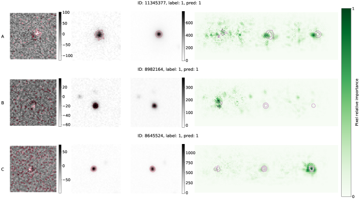
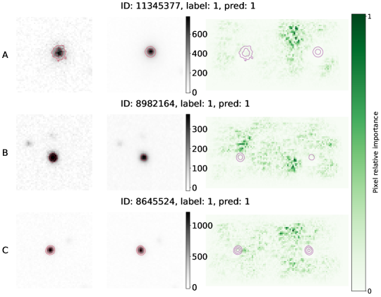
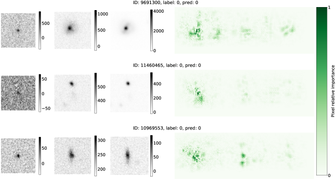
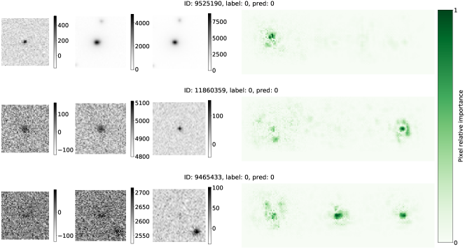
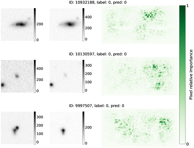
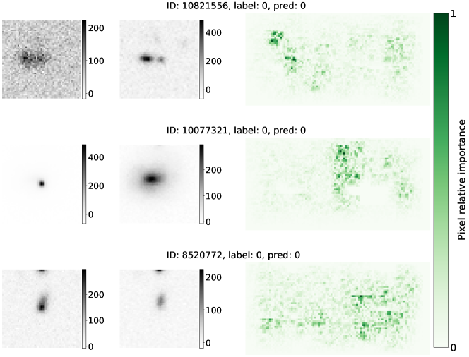
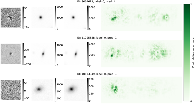
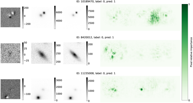
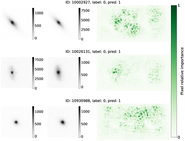
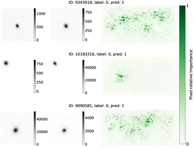
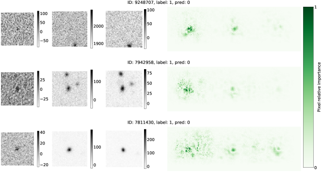
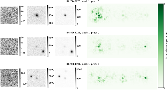
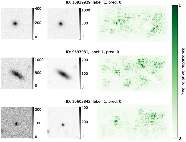
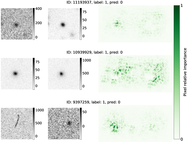
Appendix D Visual inspection of Bogus images

A total of 300 images originally label as bogus were visually inspected by our team, each inspected by 1-5 people. It was found that $\sim 3\%$ of them should be re-labeled as real and a classification disagreement persisted for $\sim 10\%$ of them.

Some of the models’ false positives were also visually inspected. A few examples are shown in Figure 23.