Quantitative Gaussian Approximation of Randomly Initialized Deep Neural Networks
Abstract.
Given any deep fully connected neural network, initialized with random Gaussian parameters, we bound from above the quadratic Wasserstein distance between its output distribution and a suitable Gaussian process. Our explicit inequalities indicate how the hidden and output layers sizes affect the Gaussian behaviour of the network and quantitatively recover the distributional convergence results in the wide limit, i.e., if all the hidden layers sizes become large.
Key words and phrases:
Neural Networks, Central Limit Theorem, Wasserstein distance2010 Mathematics Subject Classification:
60F05, 60G15, 68T991. Introduction
Contemporary machine learning has seen a surge in applications of deep neural networks, achieving state-of-the-art performances in many contexts, from speech and visual recognition [LBH15], to feature extraction and generation of samples [Goo+14]. Such a deep learning revolution [Sej18] is often compared to the advent of the industrial age [RYH22, Chapter 0], to the extent that the search for powerful and efficient steam machines historically led to the first theoretical investigations in thermodynamics. This analogy may be a bit of a stretch, but the fundamental questions about the scope and limits of deep learning methods have indeed stimulated new mathematical research in various fields, most notably probability, statistics and statistical physics, with exciting recent progresses towards enlightening answers.
1.1. Random neural networks
A successful approach focuses on the scaling limit of large neural networks whose parameters are randomly sampled. Besides the introduction of several mathematical tools, there are convincing reasons for such a study. Firstly, a Bayesian approach to machine learning problems would require a prior distribution on the set of networks, which should then be updated via Bayes rule, given the observations, e.g., the training set in supervised learning. In practice, however, large neural networks are trained via iterative optimisation algorithms [GBC16], which still require a careful initialization of the parameters, often suggested to be randomly sampled [NBS22], thus providing a second motivation for such a study. Even more strikingly, training only the parameters in the last layer of a randomly initialized neural network may still provide good performances and of course an extreme speed-up in the training algorithm, a fact that stimulated a whole machine learning paradigm [Cao+18].
In view of the above reasons, the study of random neural networks is thus not new, and in fact dates back to pioneers in the field [Ros58]. In the seminal work [Nea96], motivated by the Bayesian approach, Neal first proved that wide shallow networks, i.e., with a large number of parameters but only one hidden layer, converge to Gaussian processes, if the parameters are random and suitably tuned, as a consequence of the Central Limit Theorem (CLT). More recently, in [Mat+18, Lee+18], convergence has been extended to deeper networks, stemming a series of works that aim to explain the success story of over-parametrized neural networks, totally unexpected from traditional statistical viewpoints, by linking it to the well-established theory of Gaussian processes [WR06]. A breakthrough is the realization [Lee+19] that the training dynamics, e.g. via gradient descent, can be also traced in the scaling limit and become a differential equation of gradient flow type associated to the loss functional and the so-called Neural Tangent Kernel, i.e., a quadratic form associated to the gradient with respect to the parameters of the network, evaluated on the training set. Let us also mention the alternative perspective of the so-called mean field limit of networks [MMN18, NP21], where parameters are tuned in a Law of Large Numbers regime, leading to deterministic non-linear dynamics for the network training.
1.2. Our contribution
In this work, we provide a quantitative proof of the Gaussian behaviour of deep neural networks with random parameters at initialization, i.e., without addressing the correlations induced by the training procedure. We thus complement the seminal works [Mat+18] and subsequent ones focusing on convergence for wide networks [Yan19, Bra+20, Han21], by providing for the first time explicit rates for convergence in distribution in the case of deep networks. The metric we adopt is the Wasserstein distance, which generalizes the so-called earth mover’s distance, and provide a natural interpretation of the discrepancy between the two distributions in terms of the average cost between transporting one over the other. Indeed, it was historically introduced by Monge as the Optimal Transport problem, i.e., to efficiently move a given distribution of mass from a location to another [Vil09]. The theory of optimal transport has grown in the last decades, with applications beyond calculus of variation and probability, from geometry and partial differential equations [AGS14], to statistics and machine learning [PC+19]. We use in fact only basic properties of the Wasserstein distance, that are all recalled in Section 2.2, and focus for simplicity of the exposition only on the quadratic case, denoted by , i.e., when the transport cost between two locations is the squared Euclidean distance.
To further keep the exposition short and accessible, we discuss only so-called fully connected neural networks (or multi-layer perceptrons), where all units (neurons) in each layer are linked with those on the next layer, from the input layer to the output (see Figure 1). We denote by the total number of layers (including input and output), with sizes for the input layer, for the output and for the intermediate hidden ones. Then, for every choice of the parameters, often called weights (matrices) and biases (vectors) , and a (usually fixed) non-linear activation function acting on each intermediate node (except for the last layer), a neural network is defined (see Section 2.3 for a precise definition).
[height=4, nodesize=17pt, nodespacing=4.5em, layerspacing=3cm, layertitleheight=1em] \inputlayer[count=3, bias=false, title=Input layer, text=[count=4, bias=false, text=\hiddenlayer[count=3, bias=false, text=\outputlayer[count=2, title=Output layer, text=
Using the concepts and notation mentioned above, our main result can be stated as follows (see Theorem 3.1 for a more precise version).
Theorem 1.1.
Consider a fully connected neural network with Lipschitz activation function , and random weights and biases that are independent Gaussian random variables, centered with
| (1.1) |
Then, for every given set of inputs , the distribution of , i.e., the law of the output of the random network evaluated at the inputs , is quantitatively close to a centered multivariate Gaussian with a (computable) covariance matrix , in terms of the quadratic Wasserstein distance:
| (1.2) |
where is a constant depending on the activation function , the input and the number of layers only, not on the hidden or output layer sizes .
The random network considered in our result is also known as the Xavier initialization, which sets the initial weights using a scaling factor that takes into account the number of input and output neurons in each layer. Let us point out that several other random distributions can be considered for specific activation functions or network architectures, see [NBS22] for a review.
The matrix depends on the activation function , the input and the output dimension (not on the hidden layer sizes ). It is indeed recursively computable (see Section 2.4) and in some cases – e.g. for ReLU activation – closed formulas can be obtained, see [CS09, Lee+18]. An important feature is that all output neurons in the Gaussian approximation are independent and identically distributed variables (for any input) – the desirability of such property is often discussed, but let us recall that we are considering here non-trained networks.
A useful feature of our result is that it explicitly indicates how the layer sizes affect the Gaussian behaviour of the output of the network. In particular, in the wide limit where all the hidden layers sizes ’s are large (keeping and fixed) the Wasserstein distance becomes infinitesimal and convergence in distribution for fixed input set follows. Some considerations apply as well in the narrow deep limit, since the constant in (1.2) can be made explicit and also more general variances in (1.1) can be introduced: the contribution naturally associated to the -th hidden layer is weighted by exponentially contracting (or growing) terms as becomes large (see Remark 3.2).
1.3. Related literature
Our proof is based on the natural idea, already present in [Nea96], that the Gaussian limit emerges due to a combination, in each layer, of the CLT scaling for the weights parameters and the inherited convergence in the previous layer, which almost yields independence for the neurons. For shallow networks, which correspond to the base case of our argument, exact independence holds and Gaussian behaviour is immediate from the CLT. When considering deeper architectures, the generalization is not immediate and [Mat+18] made use of a CLT for triangular arrays. The arguments were later simplified, e.g. via the use of characteristic functions [Bra+20] or moments [Han21], but quantitative convergence in terms of any natural distance (not only the Wasserstein one) was missing so far. It turns out in fact that using the Wasserstein distance allows for quantitatively tracking the hidden layers and yields a relatively straightforward proof by induction, where the triangle inequality is employed to obtain exact independence from the previous layers, and most terms are estimated without much effort.
Let us point out that our main result provides convergence for any finite set of -inputs of a random deep neural network. Obtaining rates for deep networks in suitable functional spaces (informally, for infinitely many inputs) seems considerably more difficult, although useful, e.g. to study architectures with bottlenecks [APH20], i.e., when some hidden layers that are purposely kept with small width, such as in autoencoders. The case of shallow networks has been addressed in [EMS21, Klu22], using Stein’s method for the quadratic Wasserstein distance in the space of squared integrable functions on the sphere. In Section 5 we hint at how one could further extend our argument to obtain bounds in functional spaces.
1.4. Extensions and future work
As already mentioned, we choose to keep technicalities at minimum by considering only the quadratic Wasserstein distance, fully connected architectures, Gaussian weights and biases and a finite subset of inputs. In view of the existing literature on the subject, we expect however that all such aspects may be relaxed, e.g., from Wasserstein distances of any order or further variants, such as the entropic regularized optimal transport [PC+19]; to more general network architectures, such as those of convolutional type [Bor19, GRA18], following e.g. the general tensor program formulation proposed in [Yan19a, YL21]; to non-Gaussian laws for the random parameters, such as discrete cases or heavy-tailed distributions like stable laws where the Gaussian CLT fails [PFF20], by using finer probabilistic tools, such as quantitative multi-dimensional CLT’s in the Wasserstein space [Bon20].
Another interesting question is whether (1.2) are sharp in some sense (eventually allowing for general non Gaussian distributions in the weights and biases parameters) and what are the properties, e.g. regularity, of the optimal transport map pushing the Gaussian law to the distribution of the output of the neural network, whose existence follows from general results [Vil09, theorem 9.4]: more precise information may help to transfer finer results from Gaussian processes to neural networks.
A further direction concerns the validity of similar quantitative approximations after the training procedure, e.g. by coupling it with the gradient flow description provided by the already mentioned Neural Tangent Kernel theory. Alternatively, one could investigate if the arguments in [Hro+20] for the exact Bayes posterior may be combined with our quantitative bounds.
1.5. Structure of the paper
Section 2 is devoted to introduce notation and basic facts about neural networks, Gaussian processes and the Wasserstein distance. Section 3 contains a more precise statement of our main result, Theorem 3.1 and its entire proof. Section 4 gives with the proof of technical Lemma 3.4, while Section 5 contains some remarks on the functional limit (i.e., for infinite input sets). Finally, in Section 6 we report the outcomes of some numerical experiments about the sharpness of our main result.
2. Notation
Given a set , we write for the set of real valued functions , and write , but also frequently use the notation , to avoid subscripts (in vectors and matrices). For a subset , we denote by its restriction to . When , then we simply write , which is the set of -dimensional vectors , while if then we write , the set of matrices . The space enjoys a natural structure of vector space with pointwise sum and product and a canonical basis with if and otherwise.
Given sets , , the tensor product operation between and defines with . The canonical basis for can be then written as . If , are finite, then any can be identified also with the space of linear transformations from to via the usual matrix product
The identity matrix is defined as , i.e., , and write or in the case of or respectively. If and and , , then, up to viewing as an element in , the following identity holds:
for every , . When , then any can be also seen as a quadratic form over : is symmetric if equals its transpose , i.e., for , and positive semidefinite if, for every finite subset the restriction of to , that we denote by (instead of ) is positive semidefinite as a matrix, i.e., for every ,
If is finite, we define the trace of as . We use this notion to define a scalar product on as
which induces the norm
yielding the Euclidean norm in case of a vectors in and the Frobenius (or Hilbert-Schmidt) norm for matrices . The tensor product is associative and the norm is multiplicative, i.e., .
Given a symmetric positive semi-definite with finite, its square root is defined via spectral theorem as where is orthogonal, i.e., and is diagonal with (the eigenvalues of ) and is the diagonal with entries being the square roots of the entries of . If , are symmetric and positive semi-definite, then [HA80, Proposition 3.2] gives
| (2.1) |
where denotes its smallest eigenvalue (possibly zero: in such a case we interpret the right hand side as ). Finally, we will use the fact that if , are both symmetric and positive-semidefinite, by interpreting the identity in .
2.1. Random variables and Gaussian processes
For a random variable with values on , write for its mean value, i.e., . The second moment of is defined as , i.e., the collection , which is symmetric and positive semi-definite. We always tacitly assume that these are well-defined. The covariance matrix of is defined as the second moment of the centered variable , which coincides with its second moment if is centered, i.e., . Recalling that , and exchanging expectation and the trace operation, we have that , hence
| (2.2) |
If is a random variable with values in , its second moment
can be viewed also as in , which is a useful point of view we often adopt.
Given a symmetric positive semi-definite , we write for the centered Gaussian distribution on with covariance (or, equivalently, second moment) , i.e., the law of any Gaussian random variable with values in , and . If is infinite, the law is Gaussian if for every finite subset , the restriction has a multivariate Gaussian law with covariance . The variable is also called a Gaussian process (or field) over .
2.2. Wasserstein distance
We recall without proof basic facts about the Wasserstein distance, referring to any monograph such as [Vil09, AGS14, PC+19, San15] for details. Let be finite. The quadratic Wasserstein distance between two probability measures , on is defined as
where the infimum runs over all the random variables , (jointly defined on some probability space) with marginal laws and . For simplicity, we allow for a slight abuse of notation and often write instead of , when we consider two random variables , with values on . In particular, it holds
| (2.3) |
With this notation, a sequence of random variables converges towards a random variable , i.e., if and only if in law together with their second moments . Given , , all with values on , the triangle inequality holds
| (2.4) |
and, if is independent of and , the following inequality holds:
| (2.5) |
The distance squared enjoys a useful convexity property, which we can state as follows: given random variables , , with values on and , taking values on some , then
| (2.6) |
Finally, if , are centered Gaussian random variables with values on ( finite), it holds
| (2.7) |
which can be easily seen by considering a standard Gaussian variable on , i.e., centered with and letting and .
2.3. Deep Neural Networks
We consider only the so-called fully connected (or multi-layer perceptron) architecture, which consists of a sequence of hidden layers stacked between the input and output layers, where each node is connected with all nodes in the subsequent layer. Let and let denote the size of the layers, so that the input belongs to and the overall network outputs a vector in . Given an activation function and a set of weights and biases (in this section they do not need to be random variables)
where, for every , one has and , we define
and recursively, for ,
where the composition will be always understood componentwise. Notice that is a function of weights and biases . Given a finite subset of inputs , we identify it with a slight abuse of notation with a matrix and consider the restrictions that we interpret also as matrices
We notice that
| (2.8) | |||
| (2.9) |
for , where denotes the vector with all entries equal to .
2.4. Neural Network Gaussian Processes
The Gaussian process associated to a wide random neural network [Lee+18] is defined merenly in terms of its covariance operator (it is centered) and ultimately depends only on the choice of the activation function , the non-negative weights and biases variances
as well as the layer dimensions. As with the construction of the network, the definitions are recursive. We first define the kernel as
It is not difficult to check that is symmetric and positive semi-definite, thus there exists a centered Gaussian process on with covariance kernel , i.e.,
For , having already defined the positive semi-definite kernel , we denote with a centered Gaussian process with covariance kernel and use it to define
which can be easily seen to be positive semi-definite. For later use, let us also introduce the kernel
| (2.10) |
Finally, given layer dimensions , the Gaussian process approximating the layer output , is defined as independent copies of , i.e., a Gaussian process on , whose covariance kernel is then . To keep notation simple, at the cost of a slight ambiguity of the notation, we also write for the (vector-valued) Gaussian process. In analogy with the notation for neural networks, given inputs , write then , which is a centered Gaussian random variable with covariance
where .
3. Proof of Main Result
We consider the fully connected architecture described in the previous section, where weights and biases are all independent Gaussian random variables, centered with variances
where . We also assume that the activation function is Lipschitz, i.e., for some finite constant
| (3.1) |
This is the case with for the common choice of ReLU activation .
We state and prove a more precise version of our main result.
Theorem 3.1.
With the above notation for the deep neural network outputs with random weights and biases, and the associated Gaussian processes evaluated at inputs , there exists positive finite constants such that, for every , it holds
| (3.2) |
Each depends upon , and only the weights .
Remark 3.2.
Inequality (3.2) is evidently more precise than (1.2). In particular, besides recovering the Gaussian convergence of the network outputs (for a finite input set) in the wide limit, i.e., if all become large, it allows for some partial consideration in the deep limit, i.e., if becomes large and all the ’s are uniformly bounded. Let in (3.2) and assume e.g. that (as in the ReLu case) and all weights variances are constants, . The -th term in the sum is then multiplied by the exponential factor which becomes negligible as , if . According to [RYH22, Section 3.4], the “critical” case in the deep narrow limit is indeed the choice , where the network behaviour is “chaotic” (and not Gaussian), and indeed our inequality becomes ineffective.
Before we provide the proof of Theorem 3.1, which is performed by induction over , we inform the reades we extensively use tensor product notation. This is necessary to take into account the joint distributions of the various outputs, which are independent only in the Gaussian case (or in the wide network limit). The interested reader that would prefer to avoid tensor products but still have a good understanding of the argument is strongly invited to specialize our derivation to the case of a single input and a one-dimensional output.
Base case. The case is straightforward, since is a linear function of the Gaussian variable and , thus it has Gaussian law, centered with covariance
where in the last step we used the following computation which we state in a general form for later use (here we used and ).
Lemma 3.3.
For any , given , one has
| (3.3) |
where and
| (3.4) |
Proof.
The first identity is an explicit computation, using the covariance of :
The second identity follows from (2.2). ∎
Induction step. We assume that (3.2) holds for some and prove it for . To simplify the notation, we omit to write in what follows, and consider any probability space where random variables with the same laws as and are jointly defined (but we assume nothing on their joint law). We denote them as and .
Without loss of generality, we assume that the weights and biases are defined on the same space and independent of and , otherwise we enlarge it to define independent copies of and . We define auxiliary random variables
To take into account the biases, which play practically no role in our bounds, we also assume that a centered Gaussian random variable is defined on the same space, with values in and covariance
with the kernel introduced in (2.10). Without loss of generality, we also assume that is independent from , so that
is Gaussian with the same law as .
By the triangle inequality, we now split
and bound separately the two terms.
First term. We prove that
| (3.5) |
Indeed,
To proceed further, we condition upon and , so that, with in (3.4), we obtain
Finally, we use (3.1), to bound from above
and conclude with (3.5).
Second term. We prove that
| (3.6) |
for a positive finite constant depending on , and only (an explicit expression is (3.7) below).
To this aim, we use again (2.5) to remove the bias terms,
Next, we use (2.6) with , and . Indeed, conditioning upon , the random variable
has centered Gaussian law whose covariance is provided by (3.3) applied with : , where is given by
By (2.7), we bound from above
Therefore, by (2.6), we have
To conclude, we use the following lemma, whose proof is postponed in the next section.
Lemma 3.4.
Let be independent and identically distributed random variables with values in and finite fourth moment. Assuming that is not identically null, let and define the following random variable, taking values in ,
Then,
where denotes the smallest strictly positive eigenvalue of (which exists since , hence , is not identically null). The numerator in the right hand side is finite if has finite fourth moment.
Indeed, defining , i.e., , the independence assumption is satisfied, because is Gaussian centered with covariance hence and are not correlated if , which yields independence (which is then preserved after composition with ). Since is not identically null, so is hence the thesis with yields
where the finite constant is explicitly
| (3.7) |
and depends uniquely on the activation function , the input set and the weights variances . The proof of (3.6) is completed.
Conclusion. We have proved that
Recalling that we are considering any probability space where random variables with the same laws as and are defined, we consider the infimum over such spaces in the above inequality and conclude that
Using the inequality provided by the induction assumption we obtain the thesis.
4. Proof of Lemma 3.4
However, we need to take into account that may not to be strictly positive, hence in (2.1) could be null. To this aim, we diagonalize with orthogonal, and diagonal. Assuming without loss of generality that if and otherwise, for some , we consider the random variables , which are i.i.d. with second moment matrix , since
It follows that if , hence almost surely. Therefore, both and
have a block structure where only the first entries are not null. It follows that the square root has the same block structure and by appling (2.1) only to these blocks we obtain
where is strictly positive.
To conclude, we use that is orthogonal to obtain that
as well as the fact that the invariance of the norm (for every . Thus,
squaring both sides and taking expectation the thesis follows.
5. Some remarks on the functional limit
A natural question is to let in (1.2), or to consider more generally the neural network (and the Gaussian process) as random variables with values in a (infinite dimensional) space of functions, such as a Hilbert space, e.g., a Lebesgue space or even a Banach space, e.g., the space of continuous functions , for a compact subset and a finite measure on , e.g., and the surface measure. The main obstacle appears to be Lemma 3.4, where we use the finite dimensionality assumption on to obtain a spectral gap, i.e., a bound from below for the smallest strictly positive eigenvalue. Indeed, in infinite dimensions the general bound (2.1) still holds but we expect than strictly positive eigenvalues of accumulate towards ( becomes a compact operator). A strategy would be to decompose the action of into two eigenspaces (corresponding respectively to large and small eigenvalues) and use (2.1) in the former space and Hölder regularity for the square root in the latter (which gives a worse bound). An alternative strategy would be to rely on the uniform regularity bounds for the process provided by Kolmogorov continuity theorem: arguing as in [Bra+20], one may prove that, for every compact , and , letting be the space of -Hölder continuous functions (with the usual norm ), then
for some constant depending on (possibly also , and weights and biases variances). A similar bound holds for the Gaussian process . Given any , one can find a finite set such that for every . Then, the triangle inequality gives
If one could jointly define and in such a way that their restrictions on the finite set satisfy (1.2) (with instead of ), it would imply an inequality of the type
where the first constant in the right hand side is independent of , while depends on through . The Wasserstein distance above is between probability distributions in with respect to the cost given by the -norm . Again, the main issue is that if then the set becomes large and we expect that the constant to diverge. It thus appears achievable, although quite technical, to derive uniform bounds on compact sets for the network process and its associated processes.
We finally mention the work [MOB20], where quantitative bounds have been obtained by considering a non-Gaussian (ridgelet) prior distribution on the network weights, that approximates the Gaussian process in the output space of the network of a shallow Bayesian Neural Network. It is proved there that any Gaussian Process whose covariance regular enough can be approximated by a Bayesian Neural Network.
6. Numerical Experiments
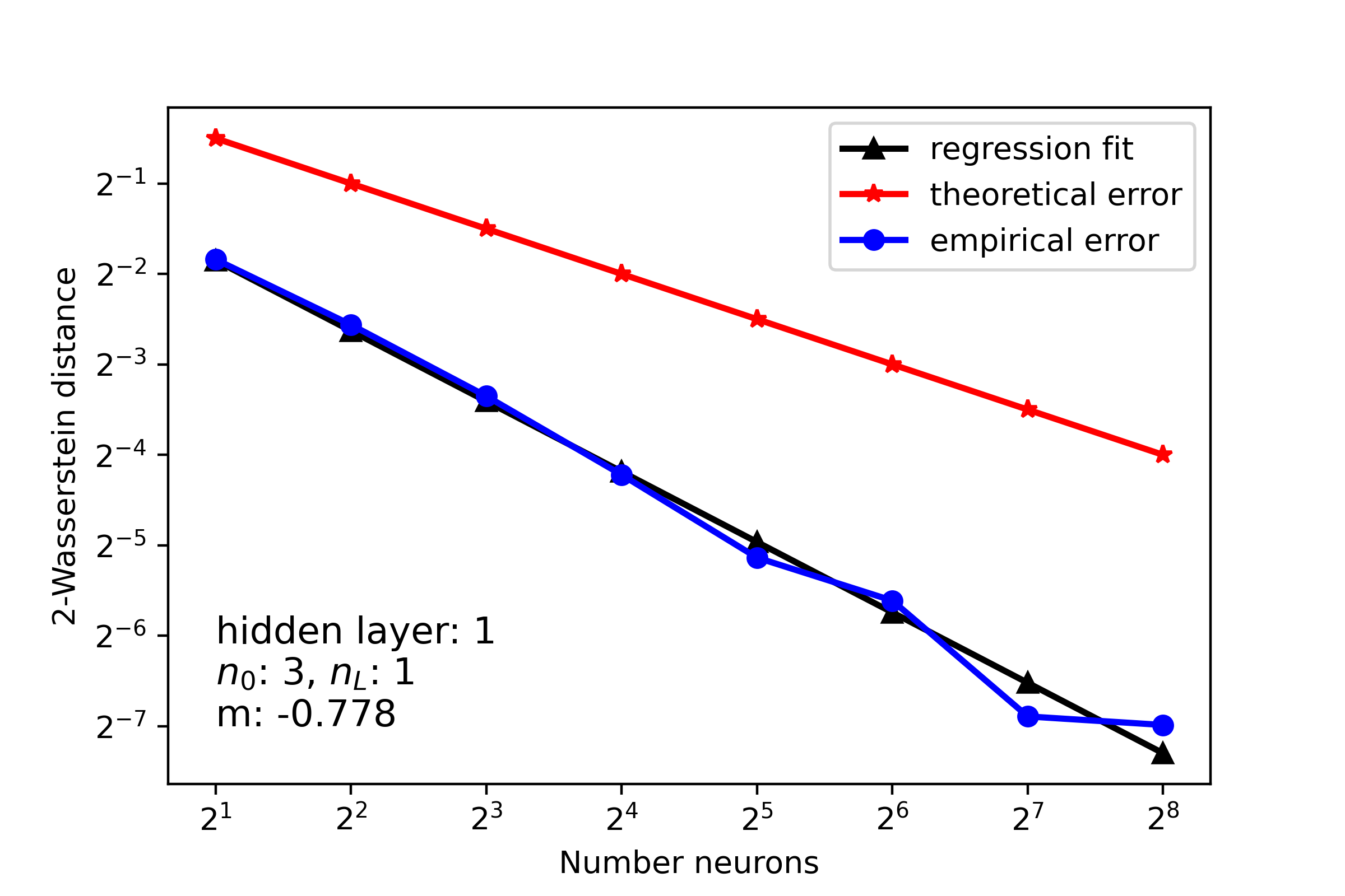
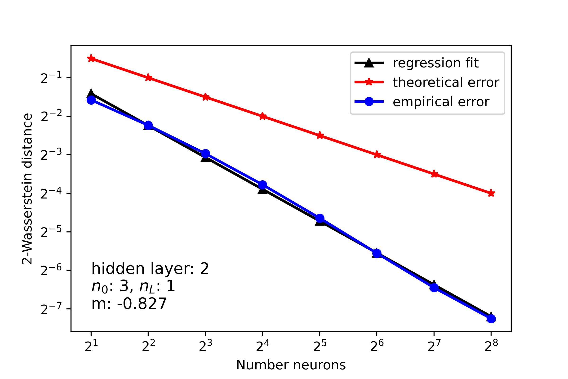
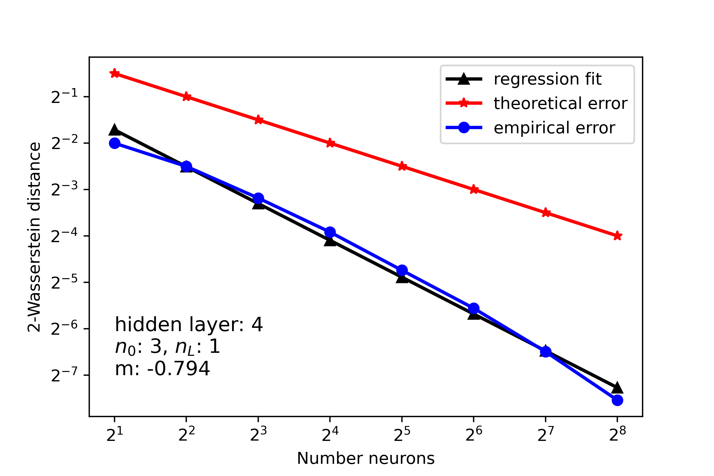
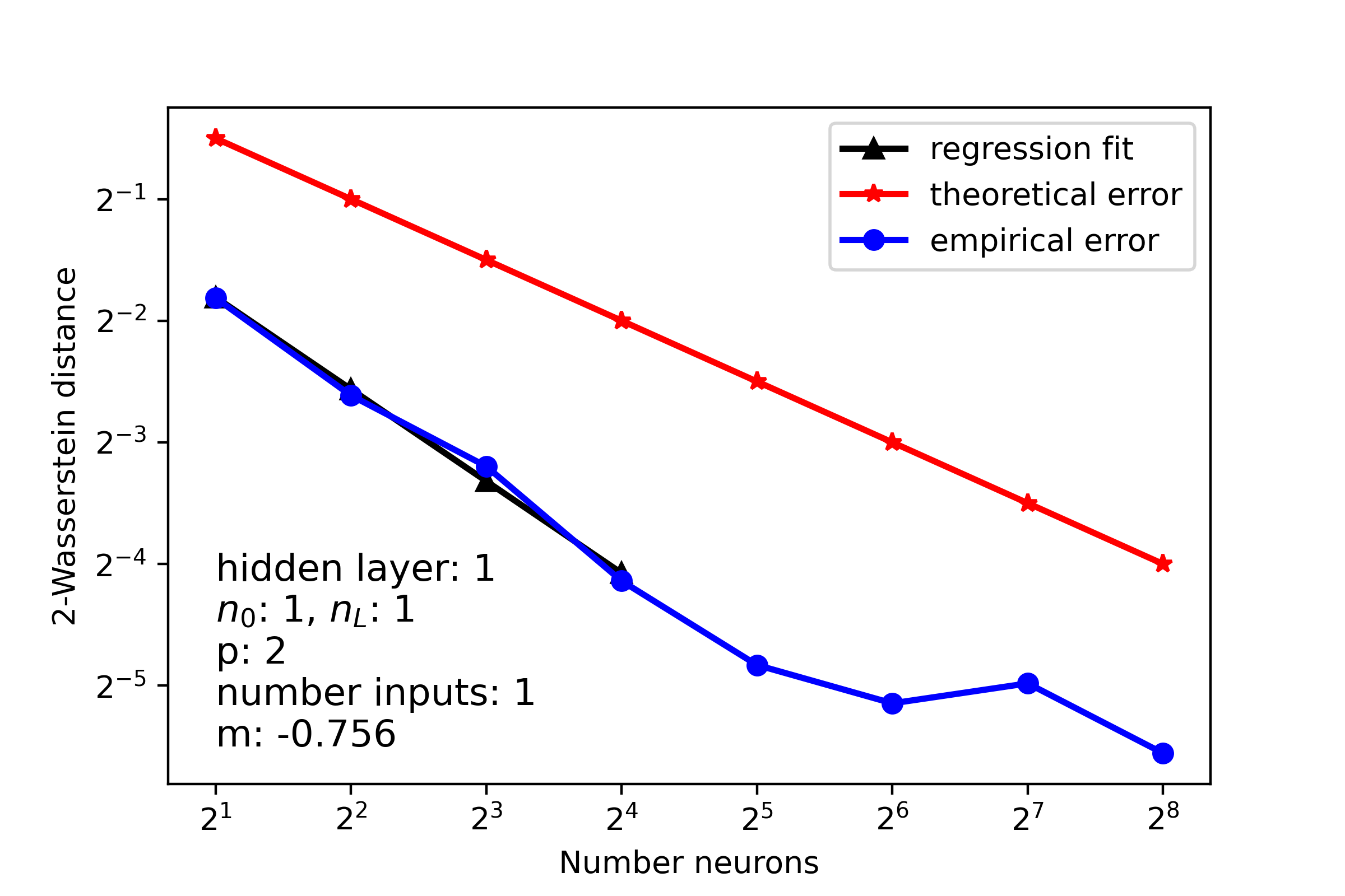
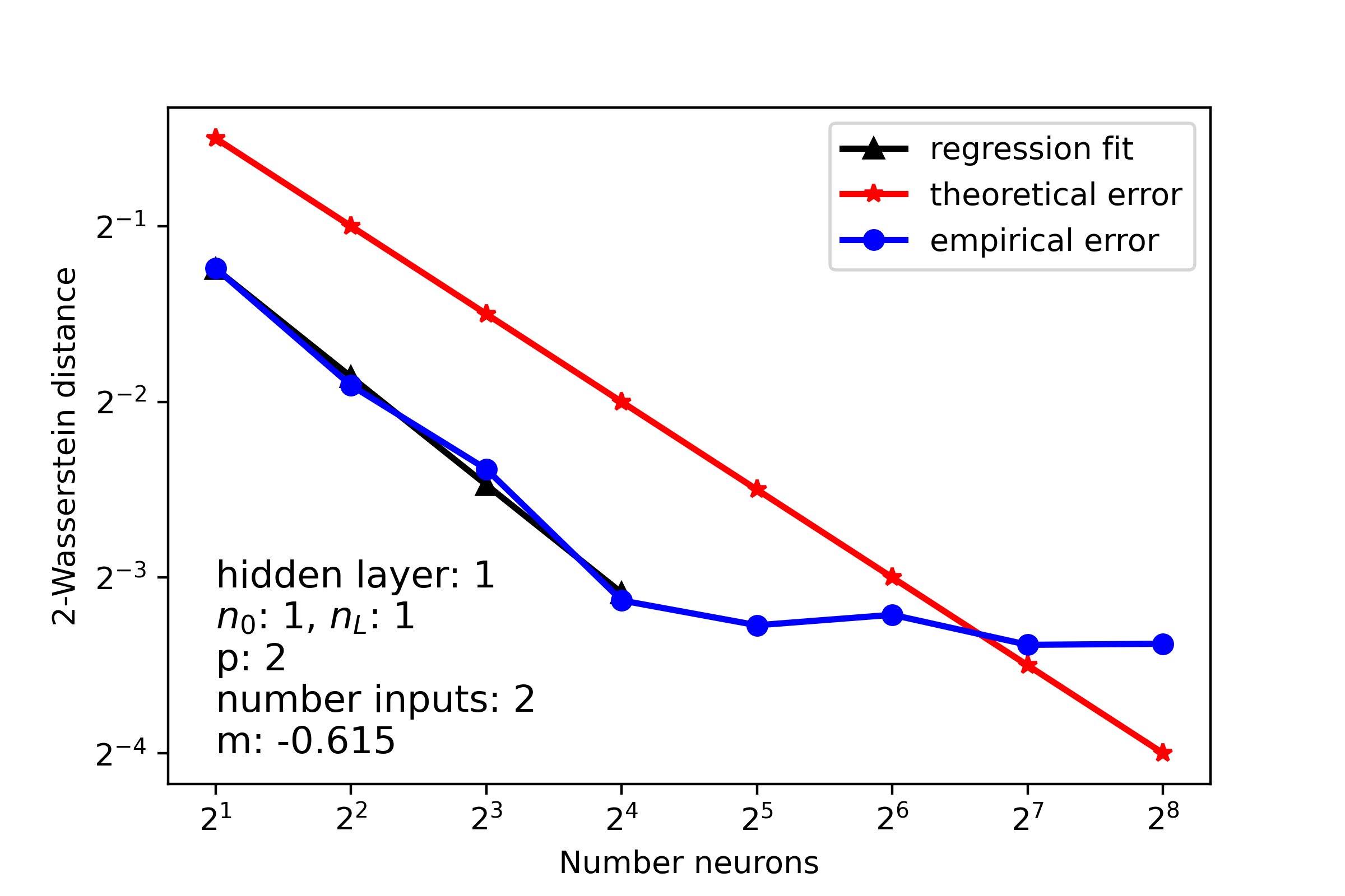
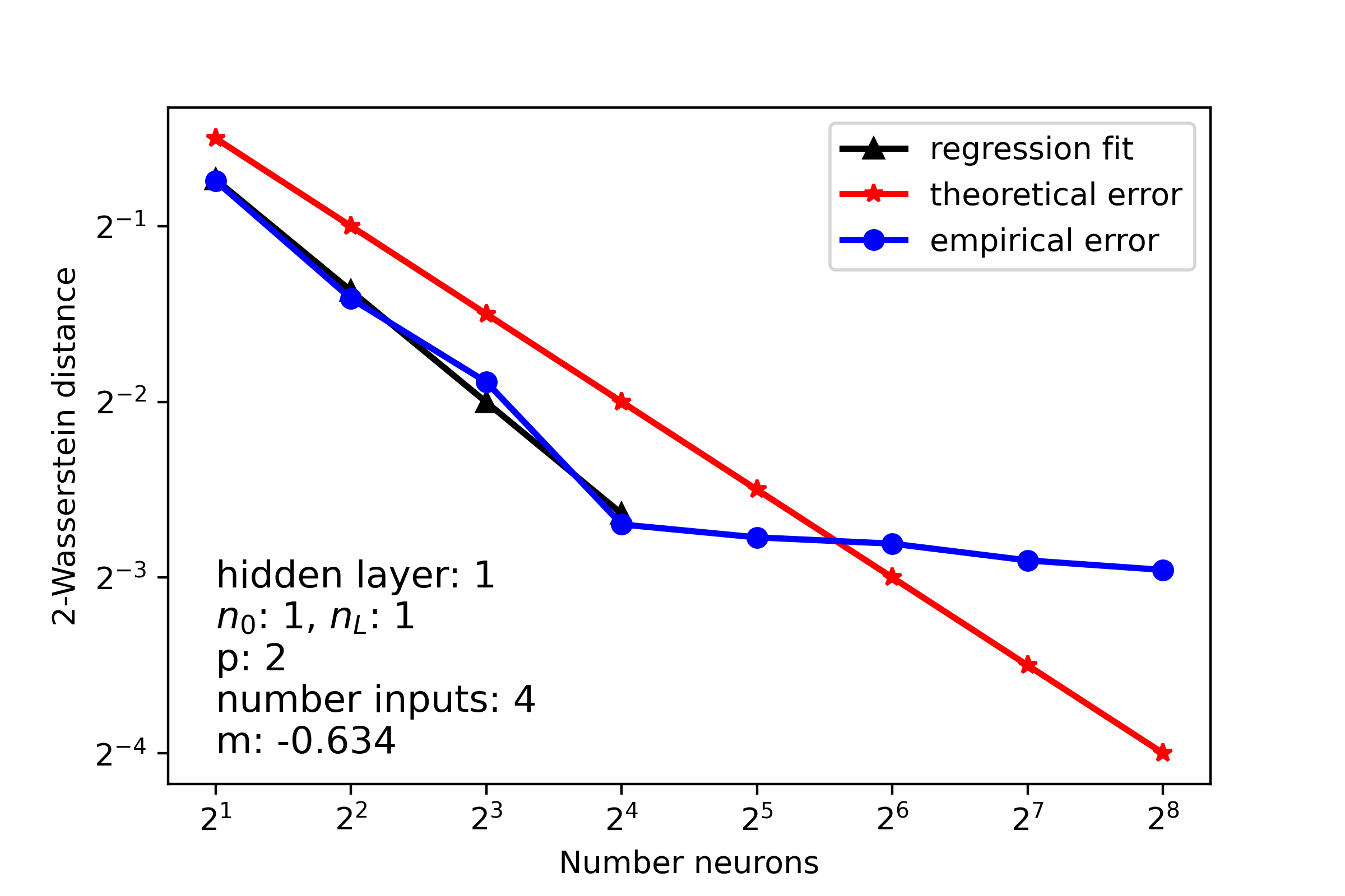
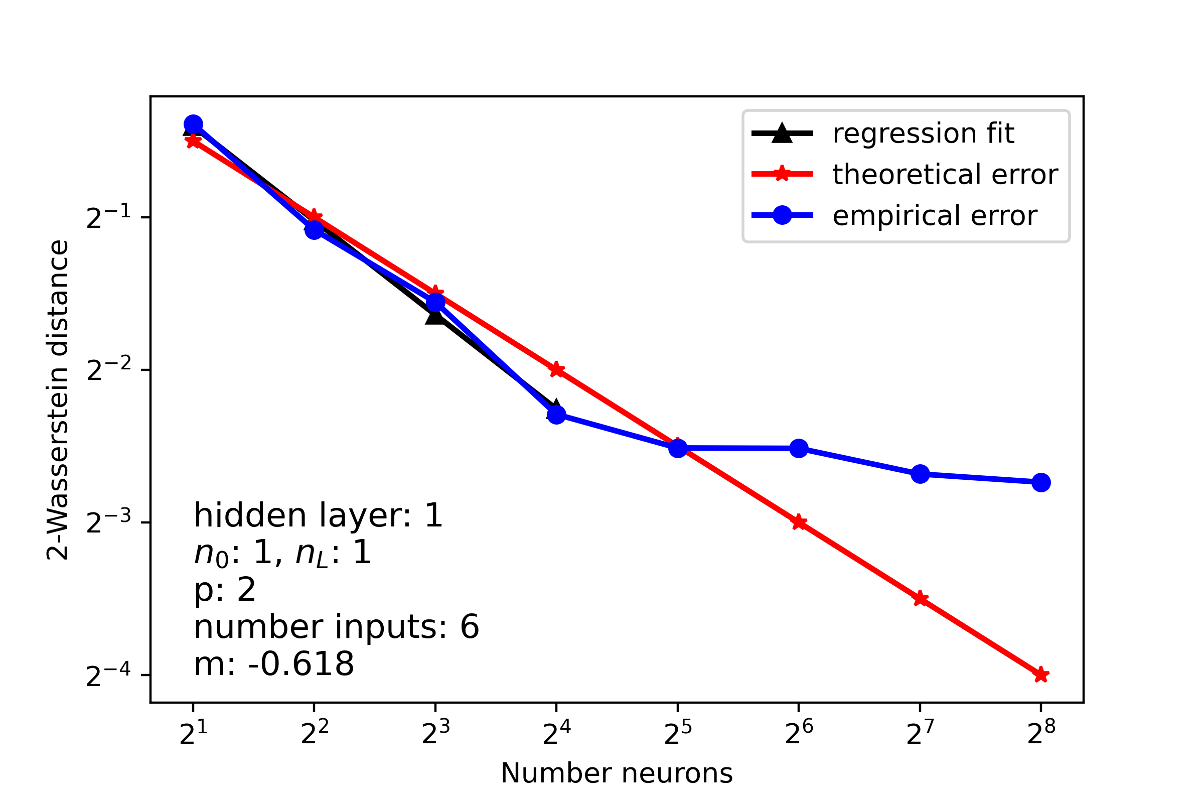
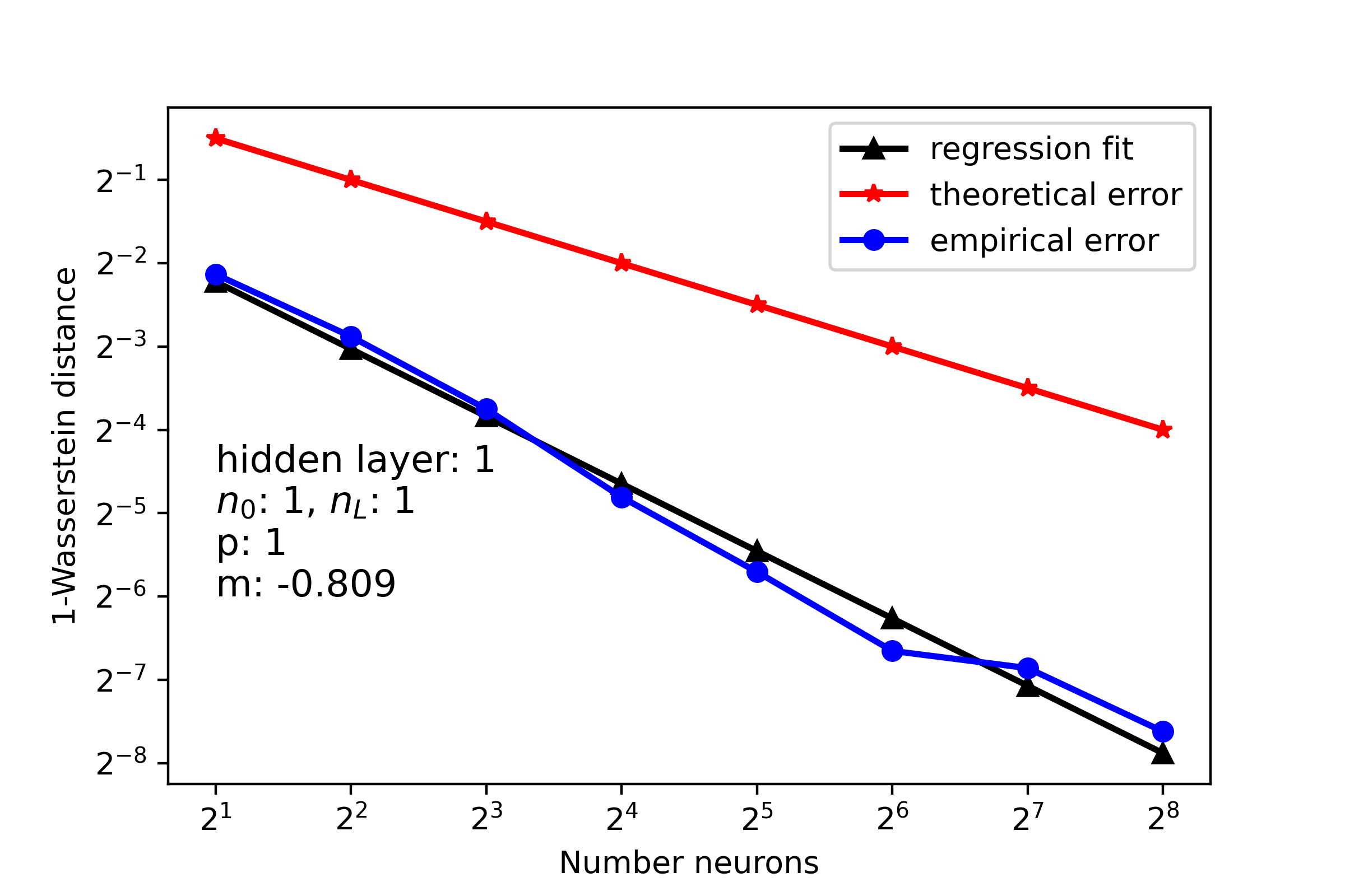
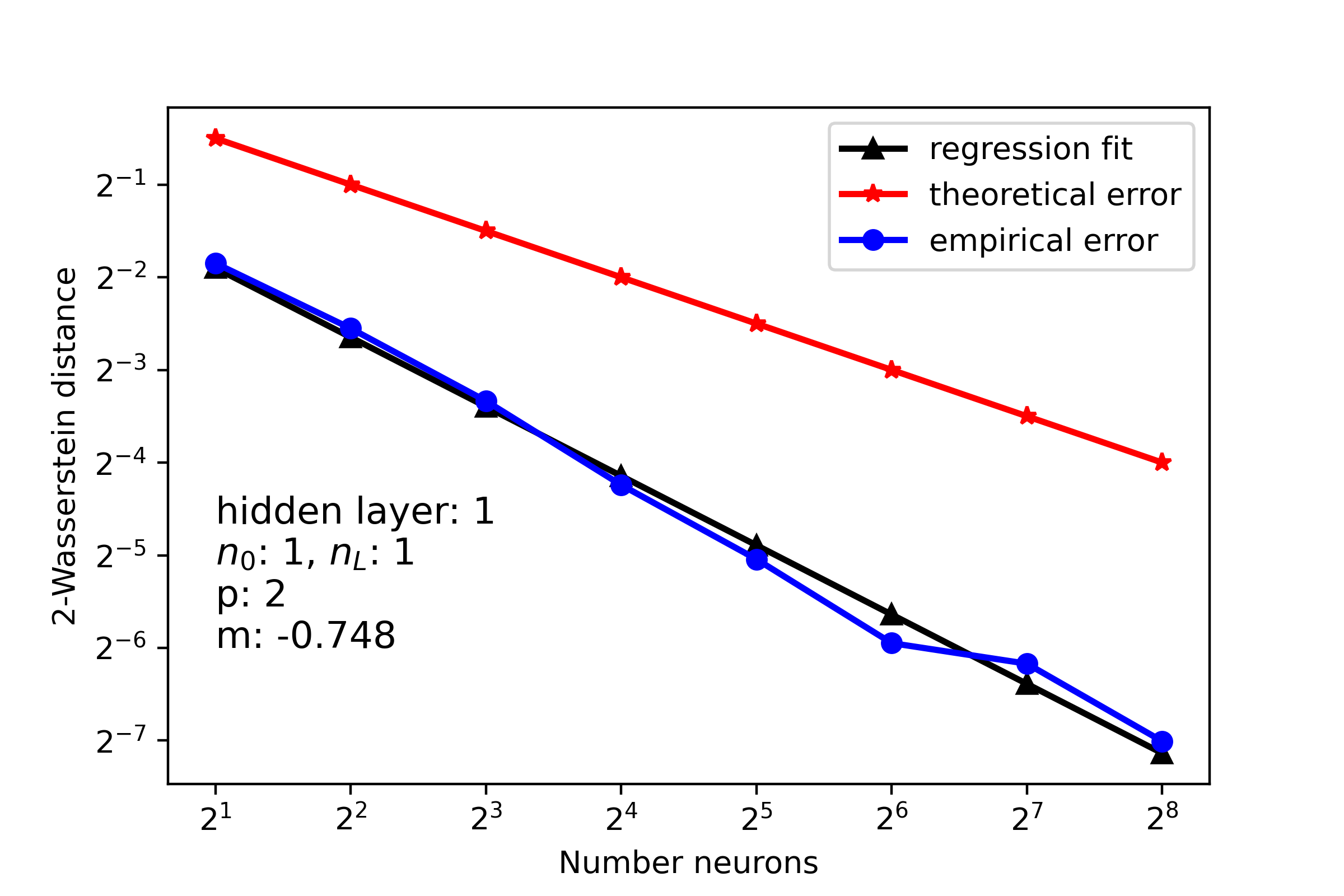
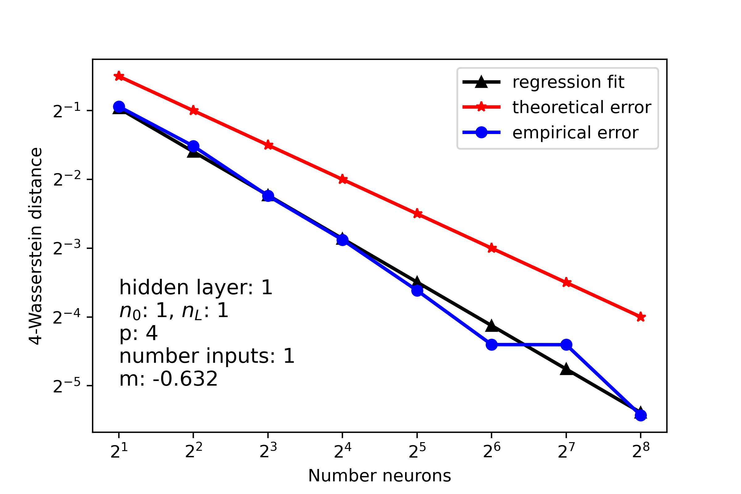
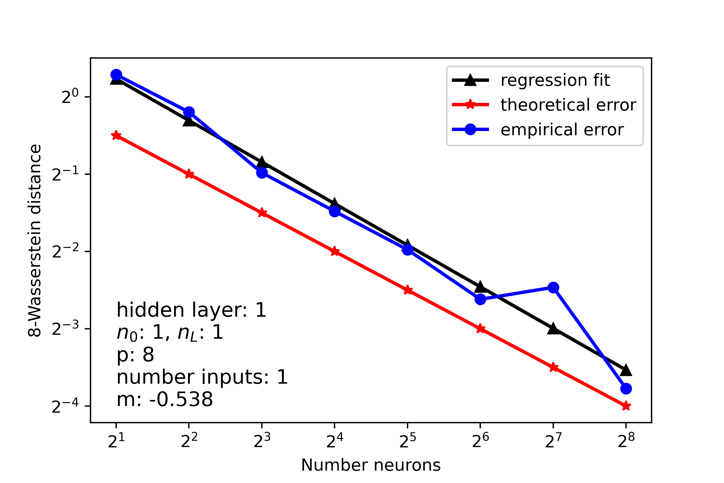
In this section we present some numerical simulations to investigate the sharpness of Theorem 1.1. The results are shown in Fig. 2, Fig. 3 and Fig. 4. Each experiment is structured as follows:
-
(1)
we fix the main parameters for a network architecture, i.e. the number of layers , the input dimension , output dimension and a set of inputs ,
-
(2)
we then set the number of neurons (i.e., the width) in the hidden layers as a parameter (for simplicity we let them be all equal),
-
(3)
we sample a large number of random Gaussian neural networks with weights sampled according to (1.1) (for simplicity we let the biases be identically zero), and for each sample we compute the output of the network at the inputs , and use the results to define the empirical distribution
-
(4)
we sample i.i.d. points from the centered multivariate Gaussian , and define a corresponding empirical distribution
-
(5)
we finally compute the Wasserstein distance between the two empirical distributions,
(6.1)
As grows, the empirical quantity (6.1) converges to the corresponding theoretical one, i.e., the left hand side of (1.2). Precisely, using e.g. the bounds from [FG15], we can approximate
where depends only on the dimension and is a suitable constant (depending on the dimension but also some mild properties of the laws, e.g. their moments). When is sufficiently large, so that the error term above is much smaller than the right hand side of (1.2), we expect an inequality of the type
for some constant .
As a rule of thumb, we need . It always holds , as dictated by the CLT, although for higher dimensions the curse of dimensionality appears, making smaller as the dimension grows. In addition to this, the exact computation of (6.1) becomes rather time-consuming, and we settled for in our experiments. We used the Python library POT: Python Optimal Transport [Fla+21] to compute the Wasserstein distance (6.1) and the neural-tangents module [Nov+20] to compute the kernel .
In the plots below, the blue lines connect the computed Wasserstein distances between the empirical distributions (in logarithmic scale as a function of the width of the hidden layers), the black line is a regression line whose slope is reported at the corner of each plot. The red line is the function and it is purely provided for reference. They all show a good agreement with our theoretical result, and may suggest even better rates of convergence, due to a fitted slope much smaller than .

7. Declarations
Funding - No funds, grants, or other support were received.
Conflicts of interest/Competing interests - Not applicable.
Ethics approval - Not applicable.
Consent to participate - Not applicable.
Consent for publication - The authors of this manuscript consent to its publication.
Availability of data and material - Not applicable.
Code availability - The code for is available upon request. Its implementation is discussed in Section 6.
Authors’ contributions - Both authors contributed equally to this work.
References
- [AGS14] Luigi Ambrosio, Nicola Gigli and Giuseppe Savaré “Metric measure spaces with Riemannian Ricci curvature bounded from below” In Duke Mathematical Journal 163.7 Duke University Press, 2014, pp. 1405–1490
- [APH20] Devanshu Agrawal, Theodore Papamarkou and Jacob Hinkle “Wide Neural Networks with Bottlenecks are Deep Gaussian Processes” In Journal of Machine Learning Research 21.175, 2020, pp. 1–66 URL: http://jmlr.org/papers/v21/20-017.html
- [Bon20] Thomas Bonis “Stein’s method for normal approximation in Wasserstein distances with application to the multivariate central limit theorem” In Probab. Theory Relat. Fields 178.3, 2020, pp. 827–860 DOI: 10.1007/s00440-020-00989-4
- [Bor19] Anastasia Borovykh “A Gaussian Process perspective on Convolutional Neural Networks” arXiv: 1810.10798 In arXiv:1810.10798 [cs, stat], 2019 URL: http://arxiv.org/abs/1810.10798
- [Bra+20] Daniele Bracale, Stefano Favaro, Sandra Fortini and Stefano Peluchetti “Large-width functional asymptotics for deep Gaussian neural networks”, 2020 URL: https://openreview.net/forum?id=0aW6lYOYB7d
- [Cao+18] Weipeng Cao, Xizhao Wang, Zhong Ming and Jinzhu Gao “A review on neural networks with random weights” In Neurocomputing 275 Elsevier, 2018, pp. 278–287
- [Cow22] Mark K. Cowan “battlesnake/neural” original-date: 2013-08-12T23:46:47Z, 2022 URL: https://github.com/battlesnake/neural
- [CS09] Youngmin Cho and Lawrence Saul “Kernel methods for deep learning” In Advances in neural information processing systems 22, 2009
- [EMS21] Ronen Eldan, Dan Mikulincer and Tselil Schramm “Non-asymptotic approximations of neural networks by Gaussian processes” In Conference on Learning Theory, 2021, pp. 1754–1775 PMLR
- [FG15] Nicolas Fournier and Arnaud Guillin “On the rate of convergence in Wasserstein distance of the empirical measure” In Probability theory and related fields 162.3-4 Springer, 2015, pp. 707–738
- [Fla+21] Rémi Flamary, Nicolas Courty, Alexandre Gramfort, Mokhtar Z Alaya, Aurélie Boisbunon, Stanislas Chambon, Laetitia Chapel, Adrien Corenflos, Kilian Fatras and Nemo Fournier “Pot: Python optimal transport” In The Journal of Machine Learning Research 22.1 JMLRORG, 2021, pp. 3571–3578
- [GBC16] Ian Goodfellow, Yoshua Bengio and Aaron Courville “Deep Learning” http://www.deeplearningbook.org MIT Press, 2016
- [Goo+14] Ian Goodfellow, Jean Pouget-Abadie, Mehdi Mirza, Bing Xu, David Warde-Farley, Sherjil Ozair, Aaron Courville and Yoshua Bengio “Generative Adversarial Nets” In Advances in Neural Information Processing Systems 27 Curran Associates, Inc., 2014 URL: https://proceedings.neurips.cc/paper/2014/hash/5ca3e9b122f61f8f06494c97b1afccf3-Abstract.html
- [GRA18] Adrià Garriga-Alonso, Carl Edward Rasmussen and Laurence Aitchison “Deep Convolutional Networks as shallow Gaussian Processes”, 2018 URL: https://openreview.net/forum?id=Bklfsi0cKm
- [HA80] J Leo Hemmen and Tsuneya Ando “An inequality for trace ideals” In Communications in Mathematical Physics 76.2 Springer, 1980, pp. 143–148
- [Han21] Boris Hanin “Random Neural Networks in the Infinite Width Limit as Gaussian Processes” arXiv: 2107.01562 In arXiv:2107.01562 [cs, math, stat], 2021 URL: http://arxiv.org/abs/2107.01562
- [Hro+20] Jiri Hron, Yasaman Bahri, Roman Novak, Jeffrey Pennington and Jascha Sohl-Dickstein “Exact posterior distributions of wide Bayesian neural networks”, 2020 URL: https://openreview.net/forum?id=s279nFs8NNT
- [Klu22] Adam Klukowski “Rate of Convergence of Polynomial Networks to Gaussian Processes” In Conference on Learning Theory, 2022, pp. 701–722 PMLR
- [LBH15] Yann LeCun, Yoshua Bengio and Geoffrey Hinton “Deep learning” Number: 7553 Publisher: Nature Publishing Group In Nature 521.7553, 2015, pp. 436–444 DOI: 10.1038/nature14539
- [Lee+18] Jaehoon Lee, Yasaman Bahri, Roman Novak, Samuel S. Schoenholz, Jeffrey Pennington and Jascha Sohl-Dickstein “Deep Neural Networks as Gaussian Processes”, 2018 URL: https://openreview.net/forum?id=B1EA-M-0Z
- [Lee+19] Jaehoon Lee, Lechao Xiao, Samuel Schoenholz, Yasaman Bahri, Roman Novak, Jascha Sohl-Dickstein and Jeffrey Pennington “Wide Neural Networks of Any Depth Evolve as Linear Models Under Gradient Descent” In Advances in Neural Information Processing Systems 32 Curran Associates, Inc., 2019 URL: https://proceedings.neurips.cc/paper/2019/hash/0d1a9651497a38d8b1c3871c84528bd4-Abstract.html
- [Mat+18] Alexander G. G. Matthews, Jiri Hron, Mark Rowland, Richard E. Turner and Zoubin Ghahramani “Gaussian Process Behaviour in Wide Deep Neural Networks”, 2018 URL: https://openreview.net/forum?id=H1-nGgWC-
- [MMN18] Song Mei, Andrea Montanari and Phan-Minh Nguyen “A mean field view of the landscape of two-layer neural networks” In Proceedings of the National Academy of Sciences 115.33, 2018, pp. E7665–E7671 DOI: 10.1073/pnas.1806579115
- [MOB20] Takuo Matsubara, Chris.. Oates and F. Briol “The Ridgelet Prior: A Covariance Function Approach to Prior Specification for Bayesian Neural Networks” In J. Mach. Learn. Res. 22, 2020, pp. 157:1–157:57 URL: https://api.semanticscholar.org/CorpusID:223956904
- [NBS22] Meenal V Narkhede, Prashant P Bartakke and Mukul S Sutaone “A review on weight initialization strategies for neural networks” In Artificial intelligence review 55.1 Springer, 2022, pp. 291–322
- [Nea96] Radford M. Neal “Priors for Infinite Networks” In Bayesian Learning for Neural Networks, Lecture Notes in Statistics New York, NY: Springer, 1996, pp. 29–53 DOI: 10.1007/978-1-4612-0745-0˙2
- [Nov+20] Roman Novak, Lechao Xiao, Jiri Hron, Jaehoon Lee, Alexander A. Alemi, Jascha Sohl-Dickstein and Samuel S. Schoenholz “Neural Tangents: Fast and Easy Infinite Neural Networks in Python” In International Conference on Learning Representations, 2020 URL: https://github.com/google/neural-tangents
- [NP21] Phan-Minh Nguyen and Huy Tuan Pham “A Rigorous Framework for the Mean Field Limit of Multilayer Neural Networks” arXiv: 2001.11443 In arXiv:2001.11443 [cond-mat, stat], 2021 URL: http://arxiv.org/abs/2001.11443
- [PC+19] Gabriel Peyré and Marco Cuturi “Computational optimal transport: With applications to data science” In Foundations and Trends® in Machine Learning 11.5-6 Now Publishers, Inc., 2019, pp. 355–607
- [PFF20] Stefano Peluchetti, Stefano Favaro and Sandra Fortini “Stable behaviour of infinitely wide deep neural networks” ISSN: 2640-3498 In Proceedings of the Twenty Third International Conference on Artificial Intelligence and Statistics PMLR, 2020, pp. 1137–1146 URL: https://proceedings.mlr.press/v108/peluchetti20b.html
- [Ros58] Frank Rosenblatt “The perceptron: a probabilistic model for information storage and organization in the brain.” In Psychological review 65.6 American Psychological Association, 1958, pp. 386
- [RYH22] Daniel A Roberts, Sho Yaida and Boris Hanin “The principles of deep learning theory” Cambridge University Press Cambridge, MA, USA, 2022
- [San15] Filippo Santambrogio “Optimal transport for applied mathematicians” In Birkäuser, NY 55.58-63 Springer, 2015, pp. 94
- [Sej18] Terrence J. Sejnowski “The Deep Learning Revolution” Google-Books-ID: 9xZxDwAAQBAJ MIT Press, 2018
- [Vil09] Cédric Villani “Optimal transport: old and new” Springer, 2009
- [WR06] CK Williams and Carl Edward Rasmussen “Gaussian processes for machine learning, vol. 2, no. 3” Cambridge, MA, USA: MIT Press, 2006
- [Yan19] Greg Yang “Wide Feedforward or Recurrent Neural Networks of Any Architecture are Gaussian Processes” In Advances in Neural Information Processing Systems 32 Curran Associates, Inc., 2019 URL: https://proceedings.neurips.cc/paper/2019/hash/5e69fda38cda2060819766569fd93aa5-Abstract.html
- [Yan19a] Greg Yang “Wide feedforward or recurrent neural networks of any architecture are gaussian processes” In Advances in Neural Information Processing Systems 32, 2019
- [YL21] Greg Yang and Etai Littwin “Tensor programs iib: Architectural universality of neural tangent kernel training dynamics” In International Conference on Machine Learning, 2021, pp. 11762–11772 PMLR