Automatic Non-Invasive Isolation of Respiratory Cycles

Abstract

In this paper, we introduce a novel algorithm designed to isolate individual respiratory cycles on a thoracic respiratory inductance plethysmography signal. The algorithm locates breaths using signal processing and statistical methods and enables the analysis of sleep data on an individual breath level. The algorithm was evaluated on 7.3 hours of hand-annotated data, or 8782 individual breaths in total, and was estimated to correctly isolate 94% of respiratory cycles while producing false positives that amount to only 5% of the total number of detections. The algorithm was specifically evaluated on data containing a great number of sleep-disordered breathing events. We found that the algorithm did not suffer in terms of accuracy when detecting breaths in the presence of sleep-disordered breathing. The algorithm was also evaluated across a large set of participants, and we found that the accuracy of the algorithm was consistent across participants. This algorithm is finally made public via an open-source Python library.

Computer aided analysis, signal processing, polysomnogram analysis, breath segmentation.

Introduction

When patients are suspected to suffer from a sleep disorder, they are recommended to undergo polysomnography (PSG), which is an overnight collection of various physiological signals, such as respiratory inductance plethysmography (RIP), oxygen saturation (SpO2), nasal airflow, electroencephalography (EEG), electromyograms (EMG), electrocardiography (ECG), audio, and others [1]. This type of study is performed either in the controlled environment of a hospital, or in a home setting, each with their advantages and disadvantages [2]. To be able to correctly detect a sleep disorder, an expert sleep scorer must manually review the PSG and annotate sleep stages and events of interest. These include respiratory events (apneas, hypopneas), oxygen desaturations, movements, and respiratory event related arousals. Finally, the annotations are used to determine the diagnosis and recommend a treatment. This manual annotation is tedious, and not all scorers will agree on a given annotation. The average agreement for sleep stages is, for example, only 82.6%[3]. There is therefore a growing need for automation and large-scale analysis in the field of sleep medicine [4].

The field of computerised scoring of PSG data mainly revolves around the analysis of fixed-length epochs, the alternative being called adaptive segmentation [5]. The main bulk of research into adaptive segmentation on polysomnography data has been in the context of examining brain activity during sleep [6], and has for example, seen some success in sleep staging [7, 8].

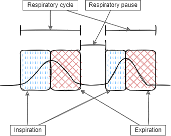
The common definition of a respiratory cycle in the literature splits a single cycle into 4 distinct phases; inspiratory, inspiratory pause, expiratory, and expiratory pause [9]. In this work, a single cycle in the respiratory system is defined as starting with an inhalation, and ending just after the following exhalation. The terms ’breath’ and ’respiratory cycle’ are considered synonyms in this work. This definition ignores the inspiratory pause phase, and interprets the expiratory pause phase rather as a pause between two individual breaths belonging to neither. Furthermore, this definition dictates that no two breaths can occupy the same moment in time. The different phases of the respiratory cycle as defined in this work are visualised in Fig. 1.

Figure 1: Phases of the respiratory cycle.

This work presents and evaluates a novel algorithm designed to locate individual respiratory cycles within a commonly collected signal in a PSG. This paper defines the term for this task as respiratory cycle isolation (RCI).

The existing literature on performing RCI is sparse, and very few papers exist that describe algorithms capable of performing the task. Moyles & Erlandson  proposed a non-parametric statistical approach to RCI, detecting changes in the trend of the air flow signal [10]. They did not perform any validation of their algorithm. Lopez-Meyer et al. presented a RCI algorithm based on peak and valley detection in the RIP signals to determine the beginning and end of a breath segment [11]. They reported a 96% precision in detecting breath cycles for participants during rest. Rosenwein et al. introduced a breath detection algorithm based on a random forest approach [12]. They derived 351 features from audio recordings and trained the model to detect inspirations and exhalations, reporting an 87% and 76% accuracy in predicting inspiration and expiration events, respectively. A Python library for RIP belt analysis and RCI exists, designed for use on people engaged in conversation, which also uses a peak and valley location algorithm to find respiratory cycles [13]. The paper describing the algorithm makes no reference to validation. Palaniappan et al. developed a neural network solution for classifying respiratory phases using respiratory sounds [14]. They reported very good overall performance for their model, but did not disclose the accuracy of the model in terms of the different phases. Finally, Hult et al. proposed a bioacoustic method that can accurately time respiration from tracheal sounds, using a summation method over the frequency domain of the audio signal. They evaluate their algorithm on 2074 respiratory cycles from two groups of participants, one being recorded in a quiet environment and another with acoustic disturbances from surrounding activities. They report detecting respiratory phases with 99% accuracy on participants in the group with the quieter environment, and approximately 90% accuracy in the group recorded with more noisy conditions.

Although the existing literature presents diverse methods for RCI algorithms, research in the field is quite limited, and the optimal solution is not known, other than a clear need for a focus on validation. A noticeable trend in the articles cited above is a lack of clarity regarding the verification and validation of the RCI algorithm they present. Some articles provide only a vague explanation how the breath placement accuracy was calculated, and some rely solely on visual observation of the output rather than objective verification. Few articles present the performance of their algorithms on data that features events such as apnea, snoring, or movement.

The existing methods of RCI are mainly based on statistics, peak and valley detection in the airflow, thoracic or abdominal RIP signals, or feature extraction and modelling, mainly done on the audio signal [10, 15, 11, 12, 13, 9, 9]. In literature, the task of RCI is sometimes referred to as breath segmentation [11, 16], or breath cycle segmentation [14], however this term leaves ambiguity on whether the segmentation is done on a respiratory phase basis, or on a respiratory cycle basis. For that reason, this paper terms the task as RCI, rather than breath segmentation.

As previously stated, the PSG contains a multitude of signals, but in the context of this paper, however, only the airflow and RIP belt signals are relevant. The airflow signal measures nasal respiration, and is most commonly measured with a pressure transducer attached to a nasal cannula, and is used to detect respiratory events [1]. The RIP signals are measured via two belts that stretch around the thorax and abdomen to measure the change in inductance caused by the movement of the body part they are placed around. RIP belts are used to detect respiratory events in conjunction with the nasal cannula and estimate respiratory effort[1]. Although not guaranteed to be included in a PSG, the audio signal is measured with a microphone, and is commonly used for snore monitoring [1].

The main contributions this paper seeks to present are:

• Introduce a novel algorithm for performing RCI.

• Propose new methods for evaluating the performance of algorithms designed to locate events in signals.

• Present the results from the introduced algorithm using the proposed evaluation methods.

Methodology

To perform RCI, a decision must be made on which signal is most appropriate to perform the task on. The two main factors in the decision are the failure rate of the signals and any potential effects of external factors. The airflow signal was deemed inappropriate for this work because the nasal cannula has several logistical issues. The sensor can get loose, affecting the measured airflow, or the participant can start mouth breathing , bypassing the sensor completely. Multiple studies show that the nasal airflow signal exhibits poor quality in 10% of cases [17, 18]. The audio signal was also eliminated, even though some studies show the signal is not as prone to error as the other signals [18], because the signal may contain a plethora of different acoustic events such as snoring, movement-related artefacts, or various background noises which complicate the task [19]. Using RIP belts has the advantage that they are not susceptible to ambient noises, nor the bypass problem that the airflow signal may encounter. Of the two RIP belts, the thoracic RIP signal captures the action of the chest-wall muscles more closely than the abdominal signal. For the reasons listed above, the thoracic RIP signal was chosen as the most appropriate signal to perform RCI on.

Evaluation Data

An extensive evaluation of the correctness of the algorithms output is required, both during normal breathing, and other conditions that may arise during sleep. The dataset used for validation contained 31 overnight PSGs from a population of people diagnosed with obstructive sleep apnea, as well as people with no known sleep issues (VSN-14-080). Of the participants, 13 were female and 18 were male. The mean age of the participants was 47.1 years, in the range of 20 - 69 years. The mean body-mass index (BMI) was 29.9 kg/$\text{m}^{2}$ in the range of 21.6 - 49.3 kg/$\text{m}^{2}$. The mean apnea-hypopnea index (AHI) was 9.3$h^{-1}$ in the range of 0.0 to 34.8 $h^{-1}$. Due either to signal failure in the RIP signal, or errors in exporting the recordings from the proprietary NOX format to the standard European data format (EDF), 5 recordings had to be discarded. Each PSG included all standard signals, including EEG, EOG, EMG, ECG, airflow recorded with a nasal cannula, thorax and abdomen RIP belts, pulse oxymetry (SpO2), and an audio signal. The RIP belts in the dataset were recorded with a 25 $\mathit{Hz}$ sampling frequency. Additionally, esophageal pressure was recorded with a nose fed catheter [20].

The algorithm was evaluated against 39 variable-length manually annotated evaluation intervals, which further split into 2 evaluation subsets. The first set, referred to as Evaluation-Subset-A was selected to specifically contain various sleep disordered breathing (SDB) events, as well as different sleep stages. Evaluation-Subset-A contained 14 variable length intervals with the mean length of 16 minutes, in the range of 1.5 to 37.5 minutes, with the cumulative length of 225.65 seconds (3.6 hours). The SDB events in Evaluation-Subset-A included obstructive apneas, hypopneas, and increases in respiratory effort without apnea or hypopnea. Further events included in Evaluation-Subset-A were sleep stages, movements, oxygen desaturations and snoring.

These intervals, however, were only selected from one participant in the dataset, and are not representative of the general public. To address that issue, a second evaluation subset was defined, referred to as Evaluation-Subset-B, consisting of a collection of 10 minute intervals from the remaining 25 valid PSGs in the dataset. These intervals were selected randomly from each recording in order to avoid cherry-picking favourable intervals. The random selection was restricted to selecting from 1 hour after the recording starts to 1 hour before the recording ends. This was done to reduce the probability of including either the participant settling down to sleep, or moving around as they wake up.

The locations of individual breaths in both evaluation subsets were then manually marked using a custom made scoring tool programmed in Python. The manual breath annotations represented the ground truth. Of the total 39 intervals in Evaluation-Subset-A and Evaluation-Subset-B, one was found to be incorrectly manually annotated and was discarded. The algorithm was therefore evaluated on 7.3 hours of manually annotated data over 38 intervals, containing 8782 individual breaths from 26 participants.

Algorithm Design

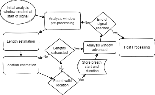
A flowchart of the proposed RCI algorithm is presented in Figure 2. The algorithm takes a thoracic RIP signal as a parameter, along with a sampling frequency $\mathit{fs}$. The output is a list of individual respiratory cycles, each consisting of the onset, i.e. the start of the respiratory cycle in seconds since the signal start, and the duration of the respiratory cycle in seconds. The algorithm works on the principle of segmenting the signal into short windows $w[n]$, with arbitrary onset $n$ in the signal, and searching for a single respiratory cycle in the selected window. The algorithm first calculates the autocorrelation function for $w[n]$ in order to estimate the lengths l of all potential breaths in the window. It then uses a probability model to discard breath length candidates that are considered too unlikely, either because the length is too long or too short. Then, for each remaining breath length l, the algorithm creates a template waveform of that length, which it correlates with the signal window to find where in the window the breath onset is most likely to be. After the window is analysed, the algorithm advances the window further in the signal, and repeats the process. The analysis windows overlap in order to allow the algorithm to analyse every breath multiple times.

Figure 2: Respiratory Cycle Isolation algorithm flowchart.

Signal Pre-processing

The preprocessing of the signal was two-fold, first the entire signal is smoothed, and then skew was removed from the signal. The RIP signal was smoothed using a Savitzky-Golay filter, which fits a polynomial function to smooth the data points [21]. The filter employed used a third order polynomial and a window size of 51. The filter parameters were tuned beforehand via experimentation to ensure that the smoothing had a minimal effect on the overall shape of the RIP signal while still eliminating some of the finer noise. Additionally, each individual $w[n]$ was corrected for skew. This was achieved by fitting a linear function to the signal in $w[n]$, then adjusting the function such that the y-intercept was 0.0. The function was then subtracted from each sample of the signal. This procedure removes large-scale skew from the signal window, but leaves the general shape of the signal intact. The procedure also had a positive effect on the template waveform fitting procedure, making it less likely to produce incorrect results due to skew. The result of this pre-processing step was that the cleaned thoracic RIP signal was ready to be used to estimate breath lengths.

Main Algorithm Body

In the first step, the algorithm takes an analysis window $w[n]$, containing a cleaned signal and estimated its periodicity $T$ using the autocorrelation function. The principle of the autocorrelation function (ACF) is to shift the signal forwards in time by $k$ and to compare it to itself. When $k=0$, the signal correlates perfectly with itself, but as $k$ increases, the correlation decreases. The formula for autocorrelation of a signal $x$ is:

$$\text{ACF}(x)[k]=\frac{1}{N}\sum_{n=0}^{N-1}x[k]\cdot x[n+k],$$ (1)

where N is the length of $x$, and $k$ the shift. For periodic signals, when $k=\frac{T}{2}$, the value of the auto correlation is low, as the signal is being compared to itself when it is in asynchony. As $k$ approaches $T$, the correlation value increases, as the first period lines up with the following period. Thus the peaks of $ACF(w[n])$ can be used to estimate the periodicity of a signal [22]. In the next step, the peaks in $ACF(w[n])$ were found using a peak-finding algorithm. Since the analysis window length was more than twice the mean breath length, $w[n]$ is likely to contain at least two breath cycles, and thus multiple peaks. To address the possibility of false alarm peaks produced by this approach, the algorithm models the breath length probabilities with a normal distribution. The parameters $\mu$ and $\sigma$ for the normal distribution were calculated as the mean and standard deviation of the length of breaths within Evaluation-Subset-A and B.

The modelled probability distribution can be seen in Figure 3 along with a density histogram of the breath lengths from the sets of 8782 manually annotated intervals.

Figure 3: Reference breath length histogram with model normal distribution.

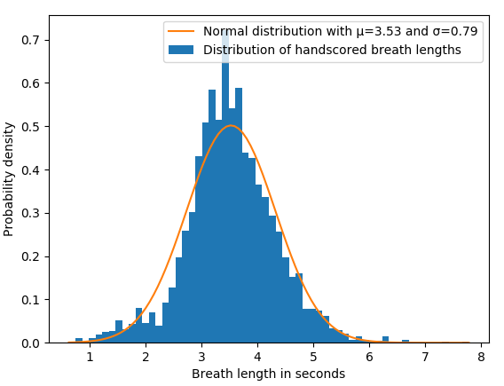
Using this probability distribution, the algorithm can rank the breath length candidates, ensuring that it considers the most probable breath length first, thus saving on computing time. Additionally, any breath length candidate whose length probability is less than three standard deviations from the mean is discarded as being too unlikely. Practically speaking, this means that any breath shorter than approximately 1 second or longer than 6 seconds was discarded.

In the next step, for every remaining breath length candidate, a discrete sine template waveform is generated, using the following formula:

$$sin[n]=sin(\frac{n*2*\pi}{l}+\theta),$$ (2)

where $l$ is the length of the candidate in seconds, and $\theta$ is an offset that can be set to 1.5 $\pi$ to shift the waveform so that it starts at -1, ends at -1, and has a peak in the middle. To find where a given template waveform fits most closely to the RIP signal window, the algorithm compares it to the RIP signal using the Pearson correlation coefficient ($\rho$) at each point on the RIP signal. The formula for calculating $\rho$ for a pair of signals is:

$$\rho\text{(w[n], sin[l])}=\frac{\text{cov(w[n], sin[l])}}{\sigma_{w[n]}\sigma_{sin[l]}}$$ (3)

where cov(w[n],sin[l]) is the covariance of the window and template waveform , and the covariance can be calculated as:

$$\text{cov(w[n], sin[l])}=\sum_{i=1}^{N}\frac{(w[n][i]-\bar{w[n]})(sin[l][i]-\bar{sin[l]})}{N}$$ (4)

where N is the length of w[n] and sin[l] which must be equal, and $\bar{w[n]}$ and $\bar{sin}$ are the means of the respective signals. The sign of $\rho$ describes whether the signals are positively or negatively correlated, and its value describes how strong the correlation is. A $\rho$ value of 0.0 means that the signals are not correlated, a value of 1.0 indicates a positive correlation, and a value of -1.0 means that the variables are perfectly inversely correlated. The algorithm treats the RIP signal as one variable and the template waveform signal as another, and calculates the correlation of the template waveform over the entire window. The correlation of the template waveform and the RIP signal produces a third signal, whose peaks represent possible onsets of the target breath.

Since the template waveform is an approximation of the shape of a breath, $\rho$ is not expected to reach 1.0. However, the correlation still provides information about the validity of the breath onset. The algorithm discards any breath onset candidate whose $\rho$ is less than 0.75. The $\rho$ elimination criterion was chosen via experimentation to eliminate as many inaccurate guesses as possible, while still not being so strict as to eliminate legitimate guesses on noisy data. If this elimination step filters out all breath onset candidates, the algorithm repeats the template waveform fitting process with another breath length candidate. If the algorithm processes all breath length candidates and no breath is found in the current signal window, then the algorithm moves on to the next window. If the correlation is above the threshold, the algorithm adds the onset and the duration to a list of breaths and moves the window onset to the end of the detected breath. This process is repeated until the signal is fully analysed.

Breath Placement Post-processing

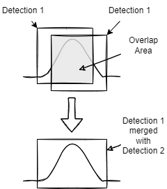
As the sliding windows overlap, the algorithm has a tendency to re-discover breaths. To solve this problem, the $i^{th}$ breath is compared to the $i+1^{th}$ breath. If the overlap of the breaths exceeds 80% of the total length, the breaths are considered a double detection, and therefore the detections are merged. The process of merging two breath detections involves replacing them with a single detection which covers the area that both previous detections covered. The percentage overlap calculation for a pair of time spans is:

$$O_{w}(A,B)=\frac{2|A{\displaystyle\cap}B|}{|A|+|B|}$$ (5)

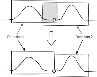
where $|A|$ and $|B|$ are the lengths of time spans $A$ and $B$ respectively, and $|A{\displaystyle\cap}B|$ is the overlap area of detections $A$ and $B$ If the breaths do not overlap at all, the value produced by this function is negative, and in the case of perfect overlap, the overlap value is 1.0. For this reason, the function is clamped above 0.0. The detection merging procedure is visualised in Fig. 4.

Figure 4: Detection merging procedure

Due to the 80% overlap required to merge breaths, the breaths can still overlap by up to 20%. By definition, a breath cannot overlap with another breath, so for each breath, the $i^{th}$ breath is compared to the $i+1^{th}$ breath. If they still overlap, the end of the $i^{th}$ and start of the $i+1^{th}$ breath are moved to the time of the minimum value of the RIP signal within the overlapping region. This process is visualised in Fig. 5.

Figure 5: Overlap elimination process (minimum of the RIP signal marked by a white circle)

The end result of this post processing process is that there is no overlapping pair of detections, satisfying the constraint that no two breaths can share a moment in time. When run on Evaluation-Subset-A and Evaluation-Subset-B, the post processing step removed 2.05% of detections on average from each interval.

Algorithm Evaluation

As the algorithm’s task was to place an individual detection anywhere on a signal, a problem presents itself when comparing detections to a ground truth. If the algorithm produces a false positive, splits a single breath into two or more breaths, or any case in which an extra detection is inserted, a misalignment between the list of detections and annotations is created where the detections placed after the false positive have an index that corresponds to the index of a later annotation than it should. The error compounds after each false positive. The same misalignment error is created when the algorithm produces a false negative, except the misalignment is now reversed, i.e., each detection after the false negative has an index corresponding to the index of an earlier annotation than it should. As with the previous case, the misalignment error compounds after each false negative.

Due to the possibility of misalignment errors, it was not possible to naively compare the list of detections and annotations, and an extra step had to be performed to match detections to their corresponding annotations. This alignment problem was solved using a matrix containing the percentage overlap of all available pairs of detections and annotations calculated using (5). This matrix is referred to as the overlap matrix and simplifies the process of finding which detection corresponds to which annotation, whether or not a given detection is a false positive or not, and whether a given annotation corresponds to a detection or is a false negative. Given an overlap matrix $A$ of a list of detections $X$ and a list of annotations $Y$, the overlap of any $X[i]$ and $Y[j]$ can be accessed in $A[i,j]$.

Using an overlap matrix, a detection corresponding to any annotation could be found by locating the index of the maximum overlap value in the overlap matrix column for that annotation. To be counted as a correct detection for a given annotation, a detection must have a weighted overlap value of over 80% with that annotation. If an annotation had no value above that threshold in its column in the overlap matrix, the breath was counted as having been missed by the algorithm (false negative). Similarly, if a detection had no value above the threshold in its row in the overlap matrix, the detection was counted as a false positive. Due to the restriction that detections may not overlap, it was impossible for two detections to correspond to the same annotation. This paper uses the precision (ratio of true positives to true positives and false positives), recall (ratio of true positives to true positives and false negatives), and F1 score metrics to estimate the accuracy of the algorithm.

In addition to the precision, recall, and F1, additional statistics were collected on the placement error of the detections that were counted as correct. Those include the length of detections vs. the length of the annotations. The start and end error was calculated using the following 2 formulae:

$$\text{start error}=s-\hat{s}\qquad\text{end error}=e-\hat{e}$$ (6)

Where $s$ is the annotation start, $e$ is the annotated breath end, $\hat{s}$ is the predicted breath start, and $\hat{e}$ is the predicted breath end.

The algorithm has 4 main parameters; the analysis window length, the overlap threshold, the correlation cut-off for the sine fitting procedure, and the probability threshold for the filtering process. To gauge the effect these variables have on the algorithms performance, the evaluation was repeated for a range of values for each variable.

Results

The algorithm was evaluated on two sets of manually annotated intervals, the first set containing a relatively high amount of SDB events, and the second set being sampled from a population of 25 participants. The results of the performance evaluation are summarised in Table I, and the placement errors are shown in Table II

Table I: Evaluation results of the RCI algorithm

Evaluation subset	Mean precision	Mean recall	Mean F1
A	0.94	0.94	0.94
B	0.93	0.95	0.94

The algorithm achieved on average 0.94 precision for Evaluation-Subset-A and 0.93 for Evaluation-Subset-B, this means that only 6%, and 7% of detections were classified as false positives for Evaluation-Subset-A and Evaluation-Subset-B respectively. The recall for Evaluation-Subset-A and Evaluation-Subset-B was 0.94 and 0.95 respectively, meaning that the algorithm only missed 6% of breaths in Evaluation-Subset-A and 5% of breaths in Evaluation-Subset-B. Two intervals in Evaluation-Subset-B had noticeably worse results, with F1 scores of 0.79 and 0.81. Upon visual inspection the errors seemed mainly to be due to incorrect manual annotations, and noise in the signal during those intervals. If these 2 intervals were omitted, the mean F1 of the algorithm increased to 0.95 for Evaluation-Subset-B. The algorithm’s performed noticeably worse for one interval in Evaluation-Subset-A than for the others, its precision being 0.76, recall being 0.963, making for an F1 score of 0.854. This was due to the interval being relatively short, and the beginning of the signal being dominated by a movement event, causing the algorithm to misclassify the movement as breaths. On the other hand, the algorithm achieved perfect precision for two intervals in Evaluation-Subset-A and one in Evaluation-Subset-B, all of which contained no SDB events, and only stable breathing. The recall was slightly more stable than the precision for both sets, with the standard deviation being 0.054 for the recall, and 0.058 for the precision.

Table II: Placement errors of the RCI algorithm.

Evaluation subset	Annotation mean breath length	Detection mean breath length	Mean abs. start error (seconds)	Mean abs. end error (seconds)
A	2.57	2.76	0.16	0.24
B.	3.56	3.88	0.23	0.30

The mean start error for both Evaluation-Subset-A and Evaluation-Subset-B was approximately 6.4% of the mean breath length. The mean end error for both sets was greater, being 10% and 8.4% of the mean breath length for Evaluation-Subset-A and Evaluation-Subset-B respectively. When visually inspected, the alignment of the detections and the thoracic RIP signal was very high for both Evaluation-Subset-A and B.

Sensitivity Analysis Results

The analysis window length was the length in seconds of the window that the algorithm searches for breaths in at each step.

Figure 6: Algorithm Recall and Precision sensitivity to window length.

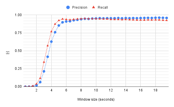
The results of the sensitivity estimation can be seen in Fig. 6, and shows that both precision and recall rise sharply as the window length reaches approximately 6 seconds, and plateaus at approximately 8 seconds. The reason for the sharp rise in performance between 2-6 seconds is most likely that the window can not reliably fit two cycles of the respiratory cycle until the window becomes longer than twice the average length of breath in the dataset.

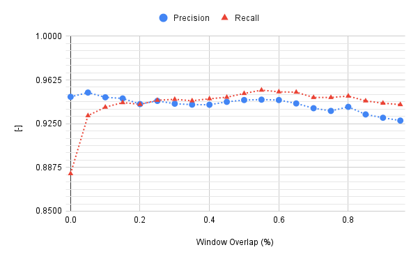
The overlap percentage is the amount of the previous window included in the next window as the analysis window advances. The effect of this parameter is shown in Fig. 7, which suggests that the algorithm performs noticeably worse only in terms of recall when the overlap percentage is around 0. This can be explained as the algorithm may miss breaths as the window skips either entirely, or partly over them. The precision seems largely unaffected, which indicates that the number of false positives drops proportionally with the number of true positives.

Figure 7: Algorithm Recall and Precision sensitivity to overlap percentage.

The correlation threshold dictates how much a breath candidate must resemble a model breath in terms of Pearson correlation (Fig. 8). It is meant to filter out waveforms that may only superficially resemble breaths, however, still forming peaks in the sine-correlation function.

Figure 8: Algorithm recall and precision sensitivity to correlation threshold.

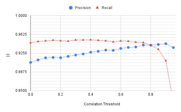
As the correlation threshold increases, the precision improves. This can be interpreted as the criterion for what "looks like a breath" becoming stricter, thus eliminating more false negatives. The recall seems unaffected by this criterion until the threshold reaches approximately 0.8, at which point it sharply drops. This is to be expected, since the template waveform is only an estimation of the general shape of a breath in the signal, and thus the correlation with the signal is not expected to be perfect.

The probability threshold parameter is used to discard breaths that are considered too unlikely. To estimate the effect of this variable on the performance of the algorithm, the evaluation was repeated for a range of probability thresholds.

Figure 9: Algorithm Recall and Precision sensitivity to probability threshold.

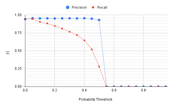
As Fig. 9 indicates, the absence of this filtering step seems to have little effect. The precision is least affected by the probability threshold, while the recall drops sharply off as the threshold increases. This is reasonable, since as the threshold increases more legitimate breaths are discarded, thus negatively affecting the recall until the threshold reaches approximately 0.55, at which point all breaths are discarded. The stability of the precision suggests that the rate of false positives drops proportionally to the rate of true positives as this parameter approaches 0.5. The reason for the falloff of both the precision and recall at 0.5 is that the maximum possible value of the probability estimator is 0.5, any value above 0.5 will therefore cause the filtering process to discard all detections.

Discussion

This paper proposes a novel algorithm designed to perform RCI on the thoracic RIP signal, based on signal processing and statistical methods. The algorithm achieved an F1 score of 0.94 when detecting breaths during sleep during both SDB events and over multiple participants, meaning that the algorithm detects around 94% of breaths correctly, with 6% false negatives. Of the detections made by the algorithm, approximately 95% are correctly placed breaths, with only 5% being false positives.

The algorithm achieved accuracy either superior [12], or comparable [11, 9] to prior work. A notable problem with comparison to prior work is that there exists no standardised method of evaluating RCI algorithms, and thus different works approach the evaluation differently, making comparison to that work difficult, if not at times impossible [14, 13, 10]. Currently, the algorithm is only evaluated on RIP signals collected with a 25Hz sampling frequency. The algorithm is designed to be independent of the sampling frequency of the signal, but requires a similarly rigorous evaluation at other sampling frequencies. In this paper, the algorithm is validated on intervals containing significant movement, respiratory events, as well as various sleep stages.

The evaluation found that the detection rate was not meaningfully influenced by respiratory events or physiology, however, the most impactful factor in terms of detection rate seemed to be artefacts. On the other hand, artefacts such as movement or signal failure only cause the algorithm to produce errors where the artefacts occur, and cause no errors for future detections, indicating that the algorithm can easily recover from a noisy period. The detection error of the correctly detected breaths is expressed in the mean absolute start and end error, the algorithm tends to produce greater end errors than start errors. The mean end error, however, was less than 8% of a mean breath length, and upon visual inspection, was not discernible to the human eye. The start and end errors of both sets may be partially explained by the fact that the manual annotations did not observe the restriction that only one breath can take place at any moment imposed by this work’s definition of the respiratory cycle, effectively introducing small sections of the annotations that at most one detection can overlap with thus negatively impacting the metrics artificially.

Despite the fact that the algorithm is originally designed for use in sleeping individuals, it could be used to research respiration during speech, exercise, emotional response analysis, and other applications, provided that the proper evaluation of the output correctness is performed. The total number of participants used for the evaluation of the algorithm was 25 individuals. In contrast to the literature, this number is comparable, as the range of the number of individuals used for testing similar tasks ranges between none reported, 4, 75, and 140 participants [10, 13, 11, 12, 14]. In future work, the algorithm should be evaluated on a much larger dataset. The algorithm is designed to work on the thoracic RIP signal, but in theory should also work on the abdominal RIP signal. However, this requires validation to assess the validity of the results.

Due to the high detection rate of the algorithm and the relatively low rate of false positives, the authors suggest that the proposed algorithm can be reliably used for future research into the nature of respiration during sleep based on RCI-based adaptive segmentation. However assessment on larger datasets is needed to evaluate the performance of the algorithm when faced with a more diverse range of respiratory events such as central apneas.

Public Availability

The algorithm described in this work has been implemented in Python, and made open-source under the GNU licence. It is available both via GitHub: github.com/benedikthth/BreathFinder, and the Python pakage manager: pypi.org/project/BreathFinder/.

[]Benedikt Holm is a Ph.D. student in Reykjavik University working with the Sleep Revolution. He received his M.Sc. degree in computer science from Reykjavik University, Reykjavik, 2021, where he worked on using machine learning to identify obstructive apnea in individual respiratory cycles. His research interests are focused on using adaptive segmentation and data science to optimise automation in sleep research.

[ ]Maria Óskarsdóttir is an Assistant Professor at the Department of Computer Science at Reykjavík University. She holds a PhD in business analytics from KU Leuven, Belgium, and a master’s degree in Mathematics from the Leibniz University Hannover, Germany. Her research is focused on practical applications of data science and analytics whereby she leverages advanced machine learning techniques, network science and various sources of data with the goal of increasing the impact of the analytics process and facilitating better usage of data science for decision making, currently focusing on sleep measurements.

[ ]Erna Sif Arnardóttir is an Assistant Professor at the Departments of Engineering, and Computer Science at Reykjavik University and the Director of the Reykjavik University Sleep Institute (RUSI). She also has an advisory position at the Landspitali – The National University Hospital of Iceland. She has over 15 years of experience within the field of clinical and scientific sleep research. Erna is the Principal Investigator in a grant from EU Horizon 2020, from 2021 to 2025. The project name is SLEEP REVOLUTION, is an inter-disciplinary and international research and development project with 37 partner institutions and companies in Europe and Australia. aim is to bring personalised medicine to sleep apnoea research, which aligns completely with the research aims of this project. Dr. Arnardóttir is the Icelandic Principal Investigator (PI) of NordSleep, a consortium project between Iceland, Finland and Norway. Her Google scholar profile shows >2000 citations, an H-index of 23 and i10-index of 32.

[ ]Marta Serwatko received her B.Sc. and M.Sc. degrees in biomedical engineering from Reykjavik University in 2013 and 2016, respectively. She has been working in sleep research since 2013 and her main research interests include sleep research and investigation of how and to what degree the disturbed sleep, due to decreased respiration, affects both adults and children, and further, what are the health consequences.

[ ]Jacqueline Clare Mallett is an Assistant Professor in RU’s Department of Computer Science. She is a multi-disciplinary computer scientist with a PhD in computer science from MIT and 30 years of industry and research experience in designing, building, and troubleshooting distributed systems, including real-time critical systems, high performance computing, signal processing, wide-area networking and computer security. She has worked on secure advanced server infrastructure for high frequency trading and consumer appliances, and teaches Computer Security at both University of Iceland and RU.

[ ]Michal Borsky is a research specialist at the RU Department of Computer Sciences. Dr. Michal Borsky has held an interest in signal processing since his master’s studies. This interest made him focus on speech recognition for his PhD degree, which he obtained at Czech Technical University in Prague. Since then, he has worked at Reykjavik University, focusing on pathological speech, and later on sleep disordered breathing and snoring. His current interests include artificial intelligence, information theory, and human biology.

References

- [1] American Academy of Sleep Medicine “International classification of sleep disorders, third edition” American Academy of Sleep Medicine, 2014
- [2] Florence Portier et al. “Evaluation of Home versus Laboratory Polysomnography in the Diagnosis of Sleep Apnea Syndrome” PMID: 10988088 In American Journal of Respiratory and Critical Care Medicine 162.3, 2000, pp. 814–818 DOI: 10.1164/ajrccm.162.3.9908002
- [3] Richard S. Rosenberg and Steven Van Hout “The American Academy of Sleep Medicine Inter-scorer Reliability Program: Sleep Stage Scoring” In Journal of Clinical Sleep Medicine 09.01, 2013, pp. 81–87
- [4] Erna Sif Arnardottir, Anna Sigridur Islind and María Óskarsdóttir “The Future of Sleep Measurements: A Review and Perspective” Sleep Medicine: Current Challenges and its Future In Sleep Medicine Clinics 16.3, 2021, pp. 447–464 DOI: https://doi.org/10.1016/j.jsmc.2021.05.004
- [5] H M Praetorius, G Bodenstein and O D Creutzfeldt “Adaptive segmentation of EEG records: a new approach to automatic EEG analysis” In Electroencephalogr. Clin. Neurophysiol. 42.1, 1977, pp. 84–94
- [6] Hartmut Schulz “Rethinking sleep analysis” In J. Clin. Sleep Med. 4.2, 2008, pp. 99–103
- [7] Aleš Procházka et al. “Adaptive segmentation of multimodal polysomnography data for sleep stages detection” In 2017 22nd International Conference on Digital Signal Processing (DSP), 2017, pp. 1–4
- [8] Henriette Koch, Poul Jennum and Julie A E Christensen “Automatic sleep classification using adaptive segmentation reveals an increased number of rapid eye movement sleep transitions” In J. Sleep Res. 28.2, 2019, pp. e12780
- [9] P Hult, B Wranne and P Ask “A bioacoustic method for timing of the different phases of the breathing cycle and monitoring of breathing frequency” In Med. Eng. Phys. 22.6 Elsevier, 2000, pp. 425–433
- [10] T.. Moyles, R.. Erlandson and T. Roth “A nonparametric statistical approach to breath segmentation” In Images of the Twenty-First Century. Proceedings of the Annual International Engineering in Medicine and Biology Society,, 1989, pp. 330–331 vol.1 DOI: 10.1109/IEMBS.1989.95756
- [11] P. Lopez-Meyer and E. Sazonov “Automatic breathing segmentation from wearable respiration sensors” In 2011 Fifth International Conference on Sensing Technology, 2011, pp. 156–160 DOI: 10.1109/ICSensT.2011.6136953
- [12] T Rosenwein, E Dafna, A Tarasiuk and Y Zigel “Detection of breathing sounds during sleep using non-contact audio recordings” In Conf. Proc. IEEE Eng. Med. Biol. Soc. 2014, 2014, pp. 1489–1492
- [13] Marcin Włodarczak “RespInPeace: Toolkit for processing respiratory belt data”, 2019 DOI: 10.5281/ZENODO.3246019
- [14] Rajkumar Palaniappan, Kenneth Sundaraj and Sebastian Sundaraj “Adaptive neuro-fuzzy inference system for breath phase detection and breath cycle segmentation” In Comput. Methods Programs Biomed. 145, 2017, pp. 67–72
- [15] Ronald D Chervin et al. “Method for detection of respiratory cycle-related EEG changes in sleep-disordered breathing” In Sleep 27.1, 2004, pp. 110–115
- [16] Benedikt Hólm Þórðarson “Analysis and detection of obstructive apnea in individual breath cycles”, 2021
- [17] F Portier et al. “Evaluation of home versus laboratory polysomnography in the diagnosis of sleep apnea syndrome” In Am. J. Respir. Crit. Care Med. 162.3 Pt 1, 2000, pp. 814–818
- [18] Ahmed S BaHammam “Signal failure of type 2 comprehensive unattended sleep studies in patients with suspected respiratory sleep disordered breathing” In Sleep Breath. 9.1, 2005, pp. 7–11
- [19] P Hult et al. “An improved bioacoustic method for monitoring of respiration” In THC 12.4, 2004, pp. 323–332
- [20] Marta Serwatko “Validation of a new method to assess respiratory effort non-invasively”, 2016 eprint: http://hdl.handle.net/1946/23804
- [21] Abraham Savitzky and M J E Golay “Smoothing and Differentiation of Data by Simplified Least Squares Procedures” In Anal. Chem. 36.8 American Chemical Society, 1964, pp. 1627–1639
- [22] Michail Vlachos, Philip Yu and Vittorio Castelli “On Periodicity Detection and Structural Periodic Similarity” In Proceedings of the 2005 SIAM International Conference on Data Mining, pp. 449–460 DOI: 10.1137/1.9781611972757.40
[![[Uncaptioned image]](/html/2203.01828/assets/Graphics/portraits/benediktbetterprofile.jpg) ]Benedikt Holm
is a Ph.D. student in Reykjavik University working with the Sleep Revolution. He received his M.Sc. degree in computer science from Reykjavik University, Reykjavik, 2021, where he worked on using machine learning to identify obstructive apnea in individual respiratory cycles. His research interests are focused on using adaptive segmentation and data science to optimise automation in sleep research.
]Benedikt Holm
[ ![[Uncaptioned image]](/html/2203.01828/assets/Graphics/portraits/maria_oskars.jpg) ]Maria Óskarsdóttir
is an Assistant Professor at the Department of Computer Science at Reykjavík University.
She holds a PhD in business analytics from KU Leuven, Belgium, and a master’s degree in Mathematics from the Leibniz University Hannover, Germany. Her research is focused on practical applications of data science and analytics whereby she leverages advanced machine learning techniques, network science and various sources of data with the goal of increasing the impact of the analytics process and facilitating better usage of data science for decision making, currently focusing on sleep measurements.
]Maria Óskarsdóttir
[ ![[Uncaptioned image]](/html/2203.01828/assets/Graphics/portraits/erna_sif.jpg) ]Erna Sif Arnardóttir
is an Assistant Professor at the Departments of Engineering, and Computer Science at Reykjavik University and the Director of the Reykjavik University Sleep Institute (RUSI).
She also has an advisory position at the Landspitali – The National University Hospital of Iceland. She has over 15 years of experience within the field of clinical and scientific sleep research.
Erna is the Principal Investigator in a grant from EU Horizon 2020, from 2021 to 2025. The project name is SLEEP REVOLUTION, is an inter-disciplinary and international research and development project with 37 partner institutions and companies in Europe and Australia. aim is to bring personalised medicine to sleep apnoea research, which aligns completely with the research aims of this project.
Dr. Arnardóttir is the Icelandic Principal Investigator (PI) of NordSleep, a consortium project between Iceland, Finland and Norway. Her Google scholar profile shows >2000 citations, an H-index of 23 and i10-index of 32.
]Erna Sif Arnardóttir
[ ![[Uncaptioned image]](/html/2203.01828/assets/Graphics/portraits/marta.jpg) ]Marta Serwatko
received her B.Sc. and M.Sc. degrees in biomedical engineering from Reykjavik University in 2013 and 2016, respectively. She has been working in sleep research since 2013 and her main research interests include sleep research and investigation of how and to what degree the disturbed sleep, due to decreased respiration, affects both adults and children, and further, what are the health consequences.
]Marta Serwatko
[ ![[Uncaptioned image]](/html/2203.01828/assets/Graphics/portraits/jacky.jpg) ]Jacqueline Clare Mallett
is an Assistant Professor in RU’s Department of Computer Science.
She is a multi-disciplinary computer scientist with a PhD in computer science from MIT and 30 years of industry and research experience in designing, building, and troubleshooting distributed systems, including real-time critical systems, high performance computing, signal processing, wide-area networking and computer security. She has worked on secure advanced server infrastructure for high frequency trading and consumer appliances, and teaches Computer Security at both University of Iceland and RU.
]Jacqueline Clare Mallett
[ ![[Uncaptioned image]](/html/2203.01828/assets/Graphics/portraits/michal.jpg) ]Michal Borsky
is a research specialist at the RU Department of Computer Sciences.
Dr. Michal Borsky has held an interest in signal processing since his master’s studies. This interest made him focus on speech recognition for his PhD degree, which he obtained at Czech Technical University in Prague. Since then, he has worked at Reykjavik University, focusing on pathological speech, and later on sleep disordered breathing and snoring. His current interests include artificial intelligence, information theory, and human biology.
]Michal Borsky