What Makes Transfer Learning Work For Medical Images:
Feature Reuse & Other Factors

Abstract

Transfer learning is a standard technique to transfer knowledge from one domain to another. For applications in medical imaging, transfer from ImageNet has become the de-facto approach, despite differences in the tasks and image characteristics between the domains. However, it is unclear what factors determine whether – and to what extent – transfer learning to the medical domain is useful. The long-standing assumption that features from the source domain get reused has recently been called into question. Through a series of experiments on several medical image benchmark datasets, we explore the relationship between transfer learning, data size, the capacity and inductive bias of the model, as well as the distance between the source and target domain. Our findings suggest that transfer learning is beneficial in most cases, and we characterize the important role feature reuse plays in its success.

1 Introduction

APTOS 2019	CBIS-DDSM	ISIC 2019	CheXpert	PatchCamelyon

Figure 1: Factors affecting the utility of transfer learning from ImageNet to medical domains. The size of each dot represents relative increase in performance ($\frac{WT}{RI}$) achieved transferring weights from ImageNet (WT) compared to random initialization (RI). The color of the dot indicates how much of the gain can be attributed to feature reuse (relative gains $\frac{WT-ST}{WT}$ from Table 1, normalized between the minimum and the maximum value for all settings, see Section 2 for details). Each panel shows the gains observed by a different model over five runs, in order of increasing inductive biases: DeiT-S, SWIN, Inception and ResNet50. The benefits from transfer learning increase with (1) reduced data size, (2) smaller distances between the source and target domain, and (3) less inductive bias. Moreover, feature reuse correlates strongly with observed gains from transfer learning, suggesting that feature reuse plays an essential role – especially for ViTs which lack the inductive biases of CNNs. (*) indicates cases where feature reuse is less important, uncovered in [36, 30].

The goal of transfer learning is to reuse knowledge gained in one domain, the source domain, to improve performance in another, the target domain. Transfer learning is often used when data from the target domain is limited. Such is the case for medical imaging, where the expense of acquisition, the rareness of the disease, as well as legal and ethical issues limit data size. The lack of large public datasets has led to the widespread adoption of transfer learning from ImageNet [10] to improve performance on medical tasks [39, 28, 27].

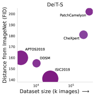
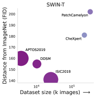
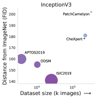
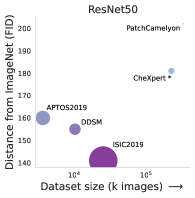
Despite its pervasive use, we do not yet fully understand what makes transfer learning from the natural to the medical domain work. In this paper, we endeavor to paint a more complete picture of which factors enable a successful transfer. Through a series of comprehensive experiments, we study the effectiveness of transfer learning as a function of dataset size, the distance from the source domain, the model’s capacity, and the model’s inductive bias. Our findings, summarized in Figure 1, show that the benefits from transfer learning increase with:

• reduced data size

• smaller distance between the source and target

• models with fewer inductive biases

• models with more capacity, to a lesser extent.

We also find a strong correlation between the observed benefits from transfer learning and evidence for feature reuse.

Much of our understanding about how transfer learning works was, until recently, based on the feature reuse hypothesis. The feature reuse hypothesis assumes that weights learned in the source domain yield features that can readily be used in the target domain. In practice, this means that weights learned on ImageNet provide useful features in the target domain, and do not change substantially during fine-tuning despite differences between the domains [4, 5, 13, 34]. This hypothesis was recently challenged when Raghu et al. demonstrated that gains observed transferring to a medical task could largely be attributed to weight scaling and low-level statistics [36], which was later confirmed in [30].

We aim to bring some clarity to the role of feature reuse in this work. Because feature reuse is difficult to measure precisely, we examine it from multiple perspectives through a series of experiments. We find that when transfer learning works well: (1) weight statistics cannot account the majority of the gains (2) evidence for feature reuse is strongest.

Our findings do not contradict those of [36, 30], rather, we show that they uncovered an isolated case (* in Figure 1) where feature reuse is less important: a large dataset, distant from ImageNet. In this scenario, transfer learning yields only marginal benefits which can largely be attributed to the weight statistics. Our work paints a more complete picture, considering datasets with more variety in size and distance to the source domain, and concludes that feature reuse plays an important role in nearly all cases.

We add to this picture with the finding that vision transformers (ViTs), a rising class of models with fewer inductive biases [11, 40], show a strong dependence on feature reuse in all the datasets we tested. We select four families of CNNs and ViTs with progressively stronger inductive biases and find that models with less inductive bias rely more heavily on feature reuse. Moreover, the pattern of feature reuse changes in models with less inductive bias. Specifically, feature reuse in ViTs is concentrated in early layers, whereas CNNs reuse features more consistently throughout the network.

We share the code to reproduce our experiments, available at github.com/ChrisMats/feature-reuse.

2 Problem Formulation and Methodology

The aim of this work is to examine transfer learning from the natural to the medical image domain. Our central question is: what factors determine if transferred representations are effective in the medical domain? Under what conditions do they yield improved performance? Is this affected by the size of the target dataset? The similarity/dissimilarity to the source dataset? What role does feature reuse play? Which of the source features are reused? And finally, what roles do the model’s architecture and inductive biases play?

To investigate these questions, we conduct a series of experiments considering a variety of medical image datasets, initialization strategies, and architectures with different levels of inductive bias. We also perform several ablation studies to characterize feature reuse at different depths throughout each network. The details of our methodology are described below.

Datasets.

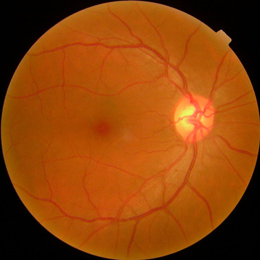
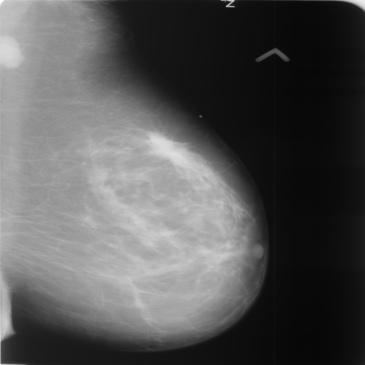
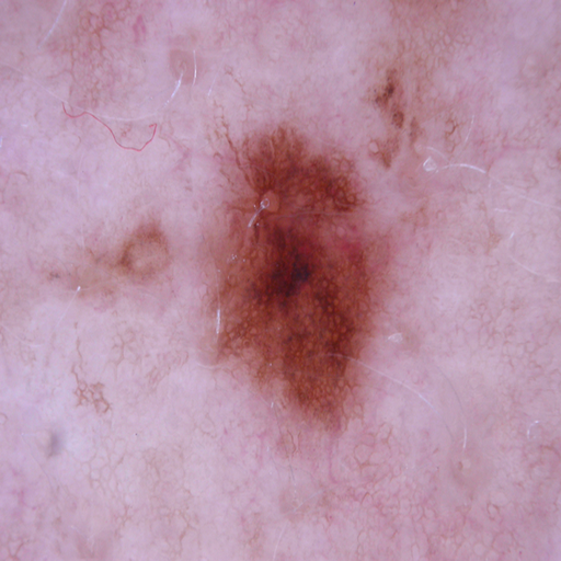
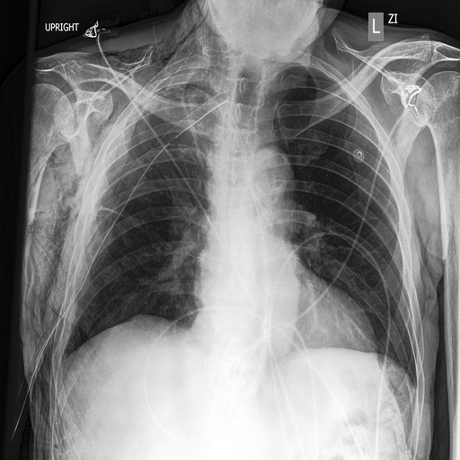
We select datasets that help us characterize how the efficacy of transfer learning varies with properties of the data. For the source domain, we use ImageNet throughout this work. For the target domain, we select a representative set of five standard medical image classification datasets. They cover a variety of imaging modalities and tasks, ranging from a few thousand examples to the largest public medical imaging datasets.

• APTOS2019 $(N=3,662)$ High-resolution diabetic retinopathy images where the task is classification into 5 categories of disease severity [19].

• CBIS-DDSM $(N=10,239)$ A mammography dataset in which the task is to detect the presence of masses [37, 23].

• ISIC 2019 $(N=25,331)$ Dermoscopic images – the task is to classify among 9 different diagnostic categories of skin lesions [41, 8, 9].

• CheXpert $(N=224,316)$ Chest X-rays with labels over 14 categories of diagnostic observations [18].

• PatchCamelyon $(N=327,680)$ Patches of H&E stained WSIs of lymph node sections. The task is to classify each patch as cancerous or normal [2, 42].

We compute the Fréchet Inception Distance (FID) [17] between ImageNet and the datasets listed above to measure similarity to the source domain (Figure 1 and Table 1). Although it may not be a perfect measure [26, 6], it gives a reasonable indication of relative distances between datasets.

Architectures.

To study the role of network architecture we selected two representative ViT models, DeiT [40] and SWIN [24], and two representative CNN models, ResNets [16] and Inception [38]. We selected these model types because they are widely studied and commonly used as backbones for other networks. To ensure a fair comparison we select architectural variants that are similar in capacity for our main experiments.

Aside from their popularity, another reason we chose these models is to study the role of inductive bias in transfer learning – as each model has a unique set of inductive biases built in. The models, in increasing order of inductive bias are: DeiT, SWIN, Inception, and ResNet. We start with the model with the least inductive biases, the DeiT family. Like the original ViT [11], DeiT is similar in spirit to a pure transformer – doing away with nearly all image-specific inductive biases, e.g. locality, translational equivariance, and hierarchical scale. According to Dosovitskiy et al., this causes pure ViTs like DeiT to generalize poorly when trained on insufficient amounts of data [11]. Recently, SWIN transformers were shown to outperform DeiTs and other ViTs on ImageNet by reintroducing many inductive biases of CNNs. Combining self-attention with a hierarchical structure that operates locally at different scales, SWIN transformers have built locality, translational equivariance, and hierarchical scale into ViTs. Moving to CNNs, we include Inception, an older CNN which features an inception block that processes the signal in parallel at multiple scales before propagating it to the next layer. Finally, we selected the ResNet family, as it is the most common and highly cited CNN backbone, and recent works have shown that ResNets are competitive with recent SOTA CNNs when modern training methods are applied [3].

Initialization methods.

To understand the mechanism driving the success of transfer learning from ImageNet to the medical domain, we need to assess to what extent improvements from transfer learning can be attributed to feature reuse. Transfer learning is typically performed by taking an architecture, along with its ImageNet pretrained weights, and then fine-tuning it on the target task. Two things are transferred via this process: the model architecture and its learned weights. Raghu et al. showed that the actual values of the weights are not always necessary for good transfer learning performance [36]. One can achieve similar performance by initializing the network using its weight statistics. In this setting, transfer amounts to providing a good range of values to randomly initialize the network – eliminating feature reuse as a factor.

To isolate the contribution of feature reuse vs. weight statistics, we employ three initialization strategies:

• Weight transfer (WT) – transferring ImageNet pre-trained weights,

• Stats transfer (ST) – sampling weights from a normal distribution whose mean and variance are taken layer-wise from an ImageNet pre-trained model,

• Random init. (RI) – Kaiming initialization [15].

Interrogating the differences between models initialized with these methods gives an indication as to what extent the transferred model reuses ImageNet features. Furthermore, we can investigate where feature reuse is beneficial within the network by transferring weights (WT) up to block $n$ and initializing the remaining $m$ blocks using ST. We denote this setup WT-ST. For example, a ResNet50 with weight transfer up to conv1 is written ResNet50-WT-ST-1/5 .

Representational similarity.

Looking more closely at feature reuse within the network, we ask the questions: how are features organized before and after fine-tuning – are they similar? Can feature similarity reveal feature reuse, or lack thereof? To answer these questions, we use Centered Kernel Alignment (CKA) to compute similarity between features within and across networks [21]. CKA’s properties of invariance to orthogonal transformations and isotropic scaling allow meaningful quantitative comparisons between representations of different size. We compute CKA pairwise between every layer (in a single network or pair of networks) to provide a visual overview of network similarity.

Resilience of the transfer.

It is difficult to directly measure whether transferred features are reused after fine-tuning. But, by investigating how “sticky” the transfer was – how much the weights drifted from their initial transferred values during fine-tuning – we can gain some insights. We use two different strategies to quantify the “stickiness” of the transfer: (1) we compute the $\ell_{2}$ distance between the initial weights and the weights after fine-tuning; (2) we measure the impact of resetting a layer’s weights to their initial values, a property called re-initialization robustness by Zhang et al. [44]. Layers that undergo critical changes during fine-tuning (and thus exhibit low robustness) have either not re-used the transferred weights well or adapted strongly to the new domain.

Analyzing transferred representations layer-wise.

The next questions we wish to address are: Which parts of the network produce/reuse low-level vs. high-level features? And how do differences in representation between CNNs and ViTs impact transfer learning? The representational power and the effective receptive field of CNNs increase with depth. ViTs, on the other hand, “see” differently [35] – they maintain more uniform representations throughout, and can utilize both local and global features at every layer.

To investigate these questions, we assess the representational power of the transferred features throughout the network. After initialization with WT, ST, and WT-ST, we fine-tune on the target dataset and apply a $k$-NN evaluation protocol at the layers in question [7]. This compares the embedded representation of test samples to the $k=200$ closest embeddings from the training set using cosine similarity. Essentially, this test allows us to see when high-level features emerge within the network. For CNNs, the embedding is obtained using global average pooling at the layer in question. For ViTs we follow a similar procedure, but with special modifications to handle the cls token in DeiTs. The cls token processes information differently than the spatial tokens, carrying much of the information necessary for classification [11, 40, 35]. Therefore we construct the embeddings in three different ways: (1) using only the cls token’s activations, (2) using activations from the spatial tokens, (3) concatenating (1) and (2).

Figure 2: Which layers benefit from feature reuse? We evaluate the impact of weight transfer when using WT-ST initialization (WT fraction from 0 to 1, where 0 = ST and 1 = WT). Lower performance on the left indicates that the network relies on transferred weights. $\star$ = RI. The last panel reports the average relative gains for each model type averaged over all datasets. Details of WT-ST initialization can be found in Appendix H.

Training procedure.

Unless otherwise specified, we used the following training procedure for all experiments. Each dataset was divided into 80/10/10 train/test/validation splits, with the exception of APTOS2019, which was divided 70/15/15 due to its small size. Images were normalised and resized to $256\times 256$ with the following augmentations applied: color jitter, random vertical and horizontal flips, and random crops $224\times 224$ after rescaling. ImageNet-pretrained weights were either available in PyTorch [33] or downloaded from the official repositories, in the cases of DeiT and SWIN. CNN and ViT models were trained with the Adam [20] and AdamW [25] optimizers respectively, with a batch size of 64. We performed independent grid searches to find suitable learning rates, and found that $10^{-4}$ works best for both CNNs and ViTs, except for RI which used $3\times 10^{-4}$. We used these as the base learning rates for the optimizers along with default 1,000 warm-up iterations. During training, we reduce the learning rate by a factor of 10 when the validation performance saturates, until we reach a final learning rate of $10^{-6}$. For transformer models, we used the default patch size of $16\times 16$ for the DeiT models and $4\times 4$ for SWIN. For each run, we save the initial checkpoint and the checkpoint with highest validation performance.

3 Experiments

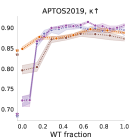
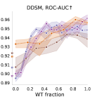
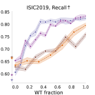
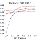
In this section, we report our findings related to transfer learning and feature reuse. Unless otherwise stated, each experiment is repeated 5 times. We report the mean and standard deviation of the appropriate evaluation metric for each dataset: Quadratic Cohen Kappa for APTOS2019, Recall for ISIC, and ROC-AUC for DDSM, CheXpert, and PatchCamelyon.

Model	Init	APTOS2019, $\kappa\uparrow$	DDSM, AUC $\uparrow$	ISIC2019, Rec. $\uparrow$	CheXpert, AUC $\uparrow$	Camelyon, AUC $\uparrow$
(# parameters)		$n=$ 3,662	$n=$ 10,239	$n=$ 25,333	$n=$ 224,316	$n=$ 327,680
		FID = 160	FID = 155	FID = 141	FID = 181	FID = 202
DeiT-S (22M)	RI	0.684 $\pm$ 0.017	0.907 $\pm$ 0.005	0.576 $\pm$ 0.013	0.740 $\pm$ 0.006	0.921 $\pm$ 0.002
	ST	0.721 $\pm$ 0.016	0.895 $\pm$ 0.005	0.607 $\pm$ 0.017	0.734 $\pm$ 0.002	0.916 $\pm$ 0.005
	WT	0.894 $\pm$ 0.017	0.949 $\pm$ 0.011	0.824 $\pm$ 0.008	0.792 $\pm$ 0.001	0.962 $\pm$ 0.003
SWIN-T (29M)	RI	0.689 $\pm$ 0.022	0.898 $\pm$ 0.005	0.597 $\pm$ 0.080	0.780 $\pm$ 0.001	0.936 $\pm$ 0.002
	ST	0.722 $\pm$ 0.017	0.900 $\pm$ 0.004	0.654 $\pm$ 0.008	0.785 $\pm$ 0.000	0.948 $\pm$ 0.013
	WT	0.906 $\pm$ 0.005	0.961 $\pm$ 0.007	0.833 $\pm$ 0.008	0.805 $\pm$ 0.000	0.968 $\pm$ 0.006
InceptionV3 (24M)	RI	0.835 $\pm$ 0.012	0.923 $\pm$ 0.003	0.668 $\pm$ 0.008	0.794 $\pm$ 0.001	0.956 $\pm$ 0.006
	ST	0.796 $\pm$ 0.014	0.907 $\pm$ 0.014	0.629 $\pm$ 0.013	0.787 $\pm$ 0.001	0.956 $\pm$ 0.003
	WT	0.873 $\pm$ 0.007	0.939 $\pm$ 0.010	0.758 $\pm$ 0.011	0.797 $\pm$ 0.000	0.958 $\pm$ 0.004
ResNet50 (25M)	RI	0.845 $\pm$ 0.022	0.919 $\pm$ 0.005	0.664 $\pm$ 0.016	0.796 $\pm$ 0.000	0.948 $\pm$ 0.008
	ST	0.848 $\pm$ 0.006	0.933 $\pm$ 0.006	0.635 $\pm$ 0.012	0.794 $\pm$ 0.001	0.959 $\pm$ 0.003
	WT	0.888 $\pm$ 0.004	0.957 $\pm$ 0.003	0.795 $\pm$ 0.011	0.800 $\pm$ 0.001	0.960 $\pm$ 0.006

Table 1: Performance of the models w.r.t different initializations.

When is transfer learning to medical domains beneficial, and how important is feature reuse?

To quantify the overall benefit of transfer learning and isolate the contribution of feature reuse, we compare weight transfer (WT), stats transfer (ST), and random initialization (RI). We also measure the distance between the source domain (ImageNet) and target domains using Fréchet Inception Distance (FID) [17]. The results are reported in Table 1 and Figure 1.

The overall trend we observe is the following: the benefits from transfer learning increase with (1) reduced data size, (2) smaller distances between the source and target domain, and (3) models with fewer inductive biases. We first consider the case where transfer learning is least beneficial: models with strong inductive biases applied to large datasets that poorly resemble ImageNet. Here, gains from transfer learning are insignificant, e.g. for ResNet50 and Inception applied to CheXpert and PatchCamelyon. The small benefits we do observe can be largely attributed to the weight statistics (ST), not feature reuse (WT), confirming previous observations [36, 30].

However, these findings do not carry over to ViTs. ViTs appear to benefit far more from feature reuse than CNNs. DeiT sees a strong boost from transfer learning on CheXpert and PatchCamelyon, wholly attributed to weight transfer, implying strong feature reuse. SWIN, which re-introduces the inductive biases of CNNs, falls somewhere in the middle. A possible explanation for this behavior is that, owing to DeiT’s lack of inductive bias, even the largest public medical datasets lack sufficient examples to learn better features than those transferred from ImageNet.

The picture changes when we turn to small datasets. Here, transfer learning shows noteworthy gains for all models. However, the strength of the gains and the importance of feature reuse depends on the inductive biases of the model and the distance between the domains. DeiT and SWIN observe significant gains across the board, strongly attributed to feature reuse. ResNet50 and Inception show reasonable gains from transfer learning on APTOS2019 and DDSM which can be partially attributed to feature reuse. Finally ISIC, the dataset which most closely resembles ImageNet, shows strong benefits for transfer learning and evidence for feature reuse for all models.

Figure 3: Layer-wise feature similarity using CKA. top: The CKA representational similarity as a function of model depth for WT initialized DeiT-S and ResNet50, before and after fine-tuning. bottom: Feature similarity between ST and WT initialized models after fine-tuning. See text for details. Full results appear in Appendix A.

Which layers benefit from feature reuse?

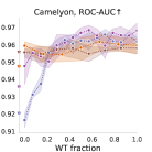
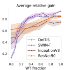
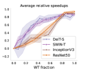
We investigate where feature reuse occurs within the network by transferring weights (WT) up to block $n$ and initializing the remaining $m$ blocks using ST. The results appear in Figure 2. Here, we see distinctive trends revealing the differences between CNNs and ViTs. On large datasets, CNNs exhibit a relatively flat line indicating that, throughout the network, weight transfer (WT) offers no benefit over the statistics (ST). Here, most of the benefits of transfer learning come from the statistics, not feature reuse. For smaller datasets, CNNs show a linear trend implying that every layer sees some modest benefit from feature reuse. DeiT shows a markedly different trend across all datasets – a sharp jump in performance in early layers – indicating a strong dependence on feature reuse in these layers. This fits with previous works that have shown that local attention, which is crucial for good performance, is learned in early layers [11, 7]. The importance of early layers we observe might be attributed to reuse of these local features which require huge amounts of data to learn [35]. SWIN exhibits properties of both DeiT and the CNNs, reflecting its mixture of inductive biases. On small datasets and those similar to ImageNet SWIN closely mirrors DeiT, but shows trends resembling a CNN with enough data. General inductive bias trends can be seen comparing models in the last panel of Figure 2 which shows the average relative gains. For ViTs, fewer inductive biases necessitates extensive feature reuse but concentrated in the early layers. CNNs benefit from reused features to a lesser extent, but more consistently throughout the network, reflecting the hierarchical nature of the architecture.

To summarize the findings thus far: the benefits of transfer learning are tied to feature reuse, and depend on the size of the dataset, proximity to ImageNet, and the model’s inductive biases. Next, we look for further evidence of feature reuse through different perspectives.

Figure 4: $\ell_{2}$ distance of weights before and after fine-tuning. We report the the mean $\ell_{2}$ distances between the initial and trained weights for different WT-ST initialization schemes, averaged over all datasets. Increased distances indicate that during training, the network larger changes the layer weights. More results can be found in Figure 17 in Appendix D.

What properties of transfer learning are revealed via feature similarity?

We investigate where similar features occur within the network using CKA, a similarity measure described in Section 2. In Figure 3 (top) and Figure 9 in the Appendix, we visualize feature similarity resulting from transfer learning (WT), before and after fine-tuning. Red indicates high feature similarity. High feature similarity along the diagonal is evidence for feature reuse in the corresponding layers. For DeiT, we see feature similarity is strongest in the early- to mid-layers. In later layers, the trained model adapts to the new task and drifts away from the ImageNet features. ResNet50 after transfer learning shows more broad feature similarity – with the exception of the final layers which must adapt to the new task. This fits with the compositional nature of CNN features, also reflected in layer-by-layer improvements in Figures 2 and 6. A common trend shared by both ViTs and CNNs is that when more data is available, the transition point from feature reuse to feature adaptation shifts towards earlier layers because the network has sufficient data to adapt more of the transferred ImageNet features to the new task.

Figure 5: Re-initialization robustness. We measure the impact of resetting the model’s weights to their initial value, one layer at a time. Drops in performance indicate that during learning, the network made critical changes to the layer weights which indicate it has not reused the transferred weights well. See text for details. Full results appear in Appendix C.

Which transferred weights change?

Another way to investigate feature reuse is to measure how much the weights drifted from their initial values during fine-tuning. In Figure 4 and Appendix D we report the $\ell_{2}$ distance between the initial weights of each network and the weights after fine-tuning. The general trend is that transferred weights (WT) remain in the same vicinity after fine-tuning, more so when transfer learning gains are strongest (Figure 17). As the network is progressively initialized more with ST, the transferred weights tend to “stick” less well. Certain layers, however, undergo substantial changes regardless – early layers in ViTs (the patchifier) and Inception, and the first block at each scale in ResNet50. These are the first layers to encounter the data, or a scale change.

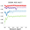
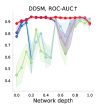
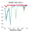
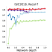
The final way we look at feature reuse is to measure the impact of resetting a layer’s weights to its initial values, or its re-initialization robustness, reported in Figure 5 and Figure 16 of the Appendix. Layers with low robustness underwent critical changes during fine-tuning. Those transferred weights could not be reused directly and had to be adapted. Our main finding is that networks with weight transfer (WT) undergo few critical changes, indicating feature reuse. When transfer learning is least effective (ResNet on CheXpert and PatchCamelyon) the gap in robustness between WT and ST is at its smallest. Interestingly, in ViTs with partial weight transfer (WT-ST), critical layers often appear at the transition between WT and ST. Rather than change the transferred weights, the network quickly adapts. But following this adaptation, no critical layers appear. As the data size increases, ViTs make more substantial early changes to adapt to the raw input (or partial WT). Transferred weights in CNNs, on the other hand, tend to be less “sticky” than ViTs. We see the same general trend where WT is the most robust, but unlike ViTs where WT was robust throughout the network, ResNet50 exhibits poor robustness at the final layers responsible for classification, and also periodically within the network at critical layers where the scale changes, as observed by [44].

Figure 6: Predictive performance of features at different depths using $k$-nn evaluation. top: $k$-NN evaluation performance at different depths for ResNet50 (row one) and DeiT-S (row two), with varying WT-ST fractions. bottom: Maximum $k$-NN evaluation score achieved at any depth for corresponding WT-ST initialization fraction, for each model type. See discussion in the text. Full results appear in Appendix B.

Are reused features low-level or high-level?

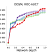
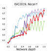
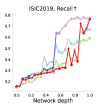
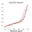
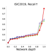
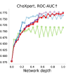
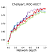
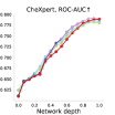
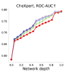
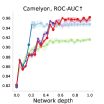
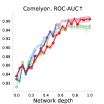
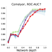
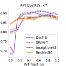
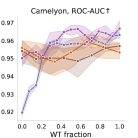
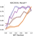
Above, we employed multiple techniques to investigate when and where feature reuse occurs within the network. With those experiments in mind, our aim now is to determine what role the reused features play. Are they low-level or high-level features? A good indicator for a high-level feature is that it can partition the data for the final task – a property we can measure layer-wise using the $k$-NN evaluation. Results of the $k$-NN test are given in Figure 6.

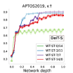
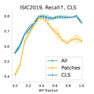
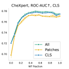
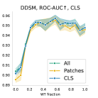
First, we consider ViTs. Previously, we observed that early layers are most crucial for ViT performance (Figure 2). In the re-initialization experiment (Figure 5) we also noticed that critical changes in ViTs occur either directly after the input, or at the transition between WT and ST. From the $k$-NN tests in Figure 6 and 16 in the Appendix, we see that the relevance of the features increases dramatically within these critical layers. Later layers do not seem to contribute further to solve the task. In the bottom of Figure 6 we notice that the discriminative power of ViT features increases rapidly as we add more WT layers in the beginning, but it saturates approximately halfway through the network. Interestingly, in an ablation we present in Appendix I, we found that the first 5 blocks of DeiTs performs comparably with the full 12 blocks for transfer learning. Evidently, early feature reuse in ViTs combined with the small medical data size results in unutilized capacity in the later layers of the ViTs, which can effectively be thrown away. Thus, we find that features reused in these critical early layers of ViTs are responsible for the creation of high-level features. According to [11, 35], these same critical early layers are responsible for learning a mix of local and global features – an essential component for good performance which requires very large datasets to learn – explaining ViT’s strong dependence on feature reuse in transfer learning. In Appendix E we confirm that WT transfer produces a mixture of local and global attention in early ViT layers, whereas ST initialization cannot learn to attend locally. Next we turn to the CKA experiments at the bottom of Figure 3. Here, we find that early layers of ST-initialized models are similar to features from the first half of the WT-initialized models. We see that if the network is denied these essential pre-trained weights, it attempts to learn them rapidly using only a few layers (due to lack of data), resulting in poor performance.

Figure 7: The impact of weight transfer for different model capacities. We evaluate the impact of weight transfer when using WT-ST initialization as a function of model capacity. Larger models benefit more from transfer learning but the same architectures follow similar patterns.

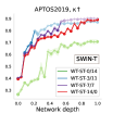
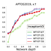
The role of transferred features in CNNs is different, as one might expect. We saw in Figure 2 that performance benefits from feature reuse are more evenly distributed throughout CNNs, while the re-initialization experiment in Figure 5 revealed that the critical layers are also spread out throughout the network. The $k$-NN test in Figure 6 further supports these findings – a jump in early layers corresponding to low-level feature extraction is followed by progressive improvements in the features as each layer adds complexity over the previous, until the final layer. Large periodic $k$-NN increases correspond to critical layers in Figure 5. These trends nicely follow our understanding of compositional learning in CNNs. A notable outlier is ISIC, where $k$-NN improvement is delayed. This is likely due to ISIC’s similarity to ImageNet, which allows mid-level transferred features to be reused more readily. From the bottom row of Figure 3 we further observe that CNNs seem to learn similar features from different initializations, suggesting that their inductive biases may somehow naturally lead to these features (although the final layers used for classification diverge). We also observe a trend where, given more data, the ST-initialization is able to learn some novel mid- to high-level features not found in ImageNet.

Capacity and convergence.

In addition to the other transfer learning factors investigated thus far we consider model capacity. We repeat our main experiments using DeiTs and ResNets with different capacities and report the results in Figure 7. We observe slight increases in transfer learning performance as model size increases, but the patterns exhibited by the individual architectures do not change.

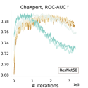
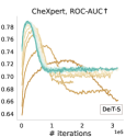
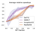
Finally, we investigate the impact of transfer learning on convergence speed. Validation curves in Figure 8 demonstrate the speed-up from transfer learning, which we measure in the last panel. We observe that convergence speed monotonically increases with the number of WT layers, in line with the finding of [36]. Furthermore, we observe that CNNs converge faster at a roughly linear rate as we include more WT layers, while vision transformers see a rapid increase in convergence speed for the first half of the network but diminishing returns are observed after that.

Figure 8: Transfer learning and convergence speed. left: Validation curves of ResNet50 and DeiT-S on CheXpert using a constant learning rate. right: Relative convergence speedups as a function of WT transferred layers. As we transfer more layers, the convergence speed of CNNs see increases linearly with the depth, while for ViTs rapid increases are observed for the first half of the network followed by a plateau.

4 Discussion

Related work.

Recent investigations have looked into which situations transfer learning works and when it fails [14, 22, 31, 12]. Kornblith et al. [22] illustrate that transferred features may be less generally applicable than previously thought. In [14], He et al. show that transfer learning does not necessarily result in performance improvements, even for similar tasks. Yosinski et al. [43] found early features tend to be more general, and as we move deeper into the network the features become more task-specific. They also showed, along with Azizpour et al., that benefits from transfer learning diminish as the distance between the source and target domain increases [1, 43]. Mustafa et al. showed that transfer learning using large architectures and orders of magnitude larger natural image pre-training datasets can yield significant improvements in medical imaging domains [29].

Most relevant to our work is the work of Raghu et al. [36], which investigates transfer learning from ImageNet to CheXpert and a large proprietary retinopathy dataset similar to APTOS2019. While they found that transfer from ImageNet provided a speed-up during training, they observed very little performance gains from transfer learning. The authors argued that the main benefits of transfer learning to the medical domain is not due to feature reuse, but rather to the weight statistics and over-parameterization of the models. Neyshabur et al. followed up their work, claiming that the observed speed-ups are due to the initialization and the low-level statistics of the data [30].

In this paper, we go beyond the previous works, providing a more comprehensive analysis that delves into feature reuse within the network. We add clarity to the previous findings by exploring a wider range of datasets, showing that transfer learning is indeed effective for smaller datasets. We consider new angles that the previous works ignored – e.g. the role of inductive biases and how transfer learning works for ViTs, as well as the how domain distance factors into transfer learning for medical images.

Factors of transferability.

In this work, we paint a more complete picture of transfer learning to the medical domain by considering more medical modalities, data sizes, and the model’s capacity and inductive bias. It is our conclusion that, for the majority of situations, transfer learning from ImageNet yields significant performance gains. Our findings do not contradict those of [36, 30], rather, we show that they uncovered an isolated case where the yields from transfer learning are minimal and feature reuse is less important.

We identify four factors that influence transfer learning from ImageNet to the medical domain. The data size and distance from the source domain are important factors that should not be overlooked. Smaller datasets always benefit from transfer learning, and so do datasets that are close to the source domain. The model’s capacity has a small effect, but inductive bias is another important factor – the benefits from transfer learning are negatively correlated with the strength of the model’s inductive biases. Looking at the extremes from our study: DeiTs, with the weakest inductive bias, heavily depend on transfer learning across the board. ResNets, the models primarily used in previous works with the strongest inductive bias, show only limited improvement for large datasets and datasets that are distant from ImageNet. But when the data size is smaller (as is often the case in medical tasks) or more similar to ImageNet, even ResNet’s benefits become significant.

The role of feature reuse.

The importance of feature reuse in transfer learning has also been recently questioned [36]. In order to better understand what drives transfer learning, we examined feature reuse from a number of different angles. Our main take-away is that when transfer learning works well, there is strong evidence of feature reuse. Beyond this, we characterized feature reuse within the network in a number of ways. We identified that certain critical features are “sticky” and less prone to change through transfer learning – though which particular features stick depends on the architecture. We observed that early layers are most crucial for ViT performance, which reuse a mixture of local and global features learned on ImageNet to perform competitively. ViT’s inability to relearn these essential features on small medical data sizes explains their strong dependence on feature reuse. We also found that this pattern of early feature reuse in ViTs means that later layers can be discarded without strongly affecting performance. CNNs benefit differently from feature reuse. In CNNs, feature reuse occurs more uniformly, marked by progressive improvements in the features as each layer adds complexity over the previous. The slope of the improvement varies with data characteristics – it can even become flat, as found in [36, 30]. We confirmed that these differences are primarily associated with model’s inductive bias, rather than capacity, through a series of ablations.

Limitations and potential negative societal impact.

An exhaustive study of the factors that impact transfer learning is impossible – countless models and datasets could have been included. Nevertheless, we tried to select relevant and representative datasets and model types, covering a more diverse selection than previously studied. A potential pitfall of this work is the use of FID [17], which may not provide a perfect measure of distance between datasets [26, 6].

Despite well-meaning intentions, applying deep learning to medical data opens the possibility of unanticipated negative impacts. Without proper consideration, models can learn to replicate unwanted biases in the data. Failures can erode the public trust, and models that operate on medical data must take care not to reveal patient information.

5 Conclusions

In this work we evaluate the benefits from transfer learning when working with medical images and how feature reuse and other factors, like the dataset and model characteristics, affect its usefulness. We show that when transfer learning works, it is because of increased reuse of learned representations, and that models with less inductive bias, small datasets and datasets that are closer to ImageNet see greater gains from it. We demonstrate that models with low inductive bias rely on reuse of local representations, composed mainly in early layers, to perform competitively with models with high inductive bias, which benefit from feature reuse throughout the network, but often to a lesser extent. Our work focuses on transfer to the medical domain, but we believe that our findings may apply to other domains, which we leave for future work.

Acknowlegements.

This work was supported by the Wallenberg Autonomous Systems Program (WASP), Stockholm County (HMT 20200958), and the Swedish Research Council (VR) 2017-04609. We thank Emir Konuk for the thoughtful discussions.

Figure 9: Feature similarity between the initial and the fine-tuned model for WT initialization. CKA feature similarity comparison between WT initialized models before and after fine-tuning. Reported for each dataset (rows) and model type (columns). Evidently, models with low inductive bias (fist two columns) indicate strong feature reuse on the early layers. On the other hand, models with strong inductive biases (last two columns) appear a more uniform pattern throughout the network. Note that for all models, more data seem to affect more high-level features.

Figure 10: Feature similarity between WT and ST fine-tuned models. CKA feature similarity comparison between WT and ST initialized models, calculated at each layer. Reported for each dataset (rows) and model type (columns). The results indicate that for models with low inductive bias, like DeiTs, the early layers of ST-initialized networks have increased similarity with early-to-mid layer features from the WT-initialized model, suggesting that the ST-initialized model learns more global features in the early layers. On the other hand, models with strong inductive biases, like ResNet50, seem to learn similar features regardless their initialization, suggesting that inductive biases may somehow naturally lead to similar features.

Figure 11: Feature similarity of WT and ST fine-tuned models for different feature-types. CKA feature similarity comparison between WT and ST initialized models in DeiT-S, using three different token types (CLS, Patches, CLS + Patches), for each dataset (columns) and embedding type (rows). Evidently, the emergence of global features in the early layers of ST initialized models is associated mainly with the patch tokens (which represent the image patches) whilst the CLS token learns different features depending on its initialization.

Appendix overview

Here, we provide further details and results from the experiments carried out in this work. Section A provides further experiment details and supplementary figures for the feature similarity experiments. Section B for the layer-wise $k$-NN evaluation experiments. Section C for the layer-wise re-initialization and Section D for the $\ell_{2}$ weight distance experiments. In Section E we show the mean attended distance for DeiT-S using different initialization schemes. In Sections F and G, we provide additional details for the convergence speed and the architectures we used to evaluate the behaviour of different model capacities. In Section H, we describe in detail the modules used for the WT-ST-$n$/$m$ initialization schemes and the intermediate layers that we used for the re-initialization, $\ell_{2}$, $k$-NN and representational similarity experiments. Finally, in Section I we provide additional details for the 5-layer DeiT-S model and we show that it performs comparably with the full 12-layer model.

Appendix A Feature similarity

Figure 12: Feature similarity between initial and fine-tuned model for ST initialization. CKA feature similarity comparison between ST initialized models before and after fine-tuning. Reported for each dataset (rows) and model type (columns). As we can see, models with no inductive biases exhibit changes throughout the network, while models with increased inductive bias focus more on the mid-to-high layers during training.

Details of the feature similarity calculations.

The feature similarity throughout this work is measured using Centered Kernel Alignment (CKA). CKA computes the feature similarity between two representations, allowing us to compare those of different layers and/or different models. For a more detailed description of CKA see [35] and [32]. The similarity scores reported in these experiments follow the procedure described in [32]. For each setting the values are calculated by measuring the similarity over the full test set, in batches of $128$. This is done for all five runs of each setting, and we report the mean similarity score averaged over all runs. The intermediate layers of the models that were used for calculating similarities could be seen in Table 2 and Table 3 in the Appendix and the results can be found in Figure 3 in the main text and Figures 9, 10, 11 and 12 in Appendix.

Appendix B $k$-NN evaluation

Figure 13: Predictive performance of features at different depths using $k$-NN evaluation. $k$-NN evaluation performance at different depths for models initialized with varying WT fractions, reported for each dataset (rows) and model type (columns). Overall the $k$-NN performance increases monotonically with depth for all models and datasets. However, relative performance gains from layer to layer exhibit different patterns. CNNs improve progressively, while ViTs increase rapidly in the beginning and then they reach a plateau. This plateau is observed to appear in association with the first ST-initialized layer in the WT-ST-$n$/$m$ experiments.

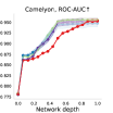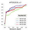
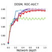
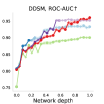
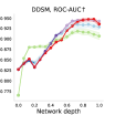
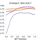
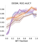
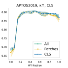
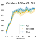
We use $k$-NN evaluation to investigate the discriminative power at different layers throughout the network.. The evaluation is performed by comparing the similarity, in the feature space, of samples from the training and the test set. In particular, we use cosine similarity as the means to calculate the distance between different data-points. Then, labels are assigned to the query data-point, from the test set, by considering its $k$ nearest neighbors from the training set. Throughout this work we use $k=200$ . The layers used to extract the embeddings are listed in Table 2 for CNNs and Table 3 for ViTs. The results of the $k$-NN evaluation experiments can be found in Figure 6 in the main text and Figures 13, 14 and 15 in the Appendix.

Figure 14: Maximum $k$-nn predictive performance of intermediate features for different WT-ST-$n$/$m$ initialization schemes. Similar to Figure 13 relative gains exhibit different patterns of improvement. Once again ViTs appear to improve quickly early on and then plateau. However, this plateau has a negative slope in some cases, suggesting the presence of strong biases in the high-level features, possibly inherited from the pre-training task.

Figure 15: Maximum $k$-nn predictive performance of intermediate features for different WT-ST-$n$/$m$ initialization schemes when using different feature types from DeiT-S for evaluation. Maximum $k$-nn evaluation score achieved at any depth for corresponding WT-ST-$n$/$m$ initialization fraction, for Deit-S (1) using only the cls token’s activations, (2) using activations from the spatial tokens, (3) concatenating (1) and (2). The different feature embeddings seem to exhibit similar trends , but the cls token often seem to outperform the patch embedding.

Appendix C Re-initialization robustness

Figure 16: Resilience of trained layers to change. We report the performance when reverting a fine-tuned layer back to its original state. This is done using one layer at a time, for each dataset (rows) and model types (columns) for four different WT-ST-$n$/$m$ initialization strategies. The results show that layers with low robustness underwent critical changes during fine-tuning. In ViTs, critical layers often appear at the transition between WT and ST. CNNs on the other hand, exhibit poor robustness at the final layers responsible for classification, and also periodically within the network at critical layers.

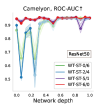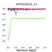
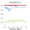
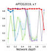
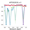
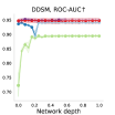
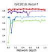
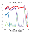
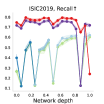
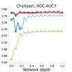
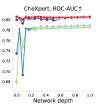
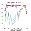
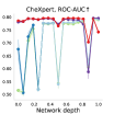
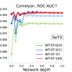
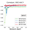
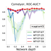
In the layer re-initialization experiments, we consider the impact of reverting individual layer of the models to their initial state. In detail, we initialize models with different WT-ST-$n$/$m$ schemes. Then, after fine-tuning, we reinitialize a single layer at a time to its original state, while keeping all the other layers unchanged. Finally, we evaluate the model on the test set and measure the drop in predictive performance.

For DeiTs and SWIN, the intermediate modules include the patchifier, the self-attention layers of each block separately. For ResNet50, the modules include the first convolutional layer and the residual blocks of each stage. For Inception the modules consist of all the initial convolutional blocks, and all the individual inception modules. A detailed description of the layers that were used can be seen in Table 2 and Table 3 in Appendix. The results of these experiments can be seen in Figure 5 in the main text for DeiT and Figure 16 for other model types.

Appendix D $\ell_{2}$ distance

In order to understand the extent that model’s weights change during training, we calculate the $\ell_{2}$ norm of the weights before and after fine-tuning. In practice, for each layer, we calculate the $\ell_{2}$ distances between the original and fine-tuned weights and then we divide this value by the number of the weights in the layer. The details of the layers used for each model can be seen in Table 2 and Table 3 in the Appendix. Figure 17 shows the the results for each model and dataset individually, and Figure 4 in the main text shows the distances averaged over all the datasets for each model.

Figure 17: $\ell_{2}$ distance of the weights. We report the the mean $\ell_{2}$ distances between the initial and trained weights for different models with different initialization schemes. A large distance indicates that the corresponding layer has changed significantly during training.

Appendix E Mean attended distance

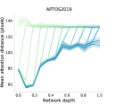
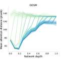
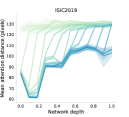
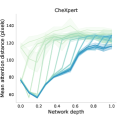
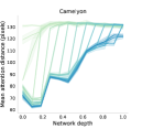
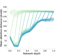
To understand the type of features that emerge at different layer depths as a function of the initialization strategy WT-ST for DeiTs, we calculate the mean attended distance per layer. That is, for each of the DeiT-S’ attention heads we calculate the mean of the element-wise multiplication of each query token’s attention and its distance from the other tokens, similarly to [11]. Then, we average the calculated distances per layer for all of the WT-ST initialization schemes. In Figure 18 in the Appendix, we report the mean attended distance per layer for all datasets and the average attended distance over all datasets. The results clearly show that (1) the ST initialization results in global attention throughout the network (2) after the critical layers the attention is mainly global (3) the WT layers introduce a mixture of local and global features. This suggests that the WT layers are important for a mixture of local and global features that the model is incapable of learning on its own – due to the small data size.

Figure 18: Mean attended distance for different initializations. We report the mean attended distance of the fine-tuned DeiT-S model for all datasets using different WT-ST initializations (WT fraction from 0 to 1, where 0 = ST and 1 = WT). The bottom-right figure shows the mean attended distance, averaged over all datasets. Evidently, in the absence of WT layers the attention is mainly global, whilst the ImageNet pre-trained weights introduce a mixture of local and global attention that the network cannot learn on its own.

Figure 19: Convergence speed as a function of WT fraction for different models and datasets. We report the number of iterations it takes for each model to converge for different WT fractions for each individual dataset. The bottom-right figure shows the relative speedups averaged over all datasets. Evidently, the convergence speed monotonically increases with the number of WT layers for all datasets and models.

Appendix F Model convergence

We investigate how the convergence behavior of the models change as we transfer more layers. Figure 19 in the Appendix and Figure 8 in the main text show the number of iterations needed for each model to reach its best validation performance. As a general trend for all models, the higher the WT fraction is, the faster the models converge. Interestingly, for vision transformers, transferring the first few blocks dramatically increases the convergence speed, while transferring further blocks slightly speeds up training. CNNs however, follow a different trend, where transferring more layers improves the convergence speed at a roughly linear rate.

Appendix G Model capacity

We investigate the impact that the model’s capacity has on transfer learning for DeiTs [40] and ResNets [16]. To this end, we consider 3 different capacities for each architecture, which are comparable in the number of parameters and compute time. For the ResNet family, we considered ResNet18, ResNet50, and ResNet152. For the DeiT family, we chose DeiT-T, DeiT-S, and DeiT-B. For each model capacity, we carry out the same WT-ST-$n$/$m$ experiments. That is, we initialize each model with different WT-ST-$n$/$m$ initialization schemes and then we fine-tune them on the target task. The training strategy follows exactly the details mentioned in Section 2. Please refer to to Figure 8 and Section 3 for the results and discussion.

Initialization for Inception		Features of Inception	Initialization for ResNets		Features of ResNet50
WT-ST-n/m	Module	Intermediate layers	WT-ST-n/m	Module	Intermediate layers
WT-ST-1/6	Layer 1	Conv2d	WT-ST-1/5	Layer 1	Conv2d
WT-ST-2/5	Layer 2	Layer 2, Conv2d	WT-ST-2/4	Norm layer (BN)
		Layer 2, Conv2d
WT-ST-3/4	Layer 3	Layer 3, Conv2d	WT-ST-3/3	Stage 1	Stage 1, Block 1
WT-ST-4/3	Layer 4	Layer 4, Conv2d			Stage 1, Block 2
					Stage 1, Block 3
WT-ST-5/2	Stage 1	Stage 1, Block 1 – Type A	WT-ST-4/2	Stage 2	Stage 2, Block 1
		Stage 1, Block 3 – Type A			Stage 2, Block 2
		Stage 1, Block 3 – Type A			Stage 2, Block 3
					Stage 2, Block 4
WT-ST-6/1	Stage 2	Stage 2, Block 1 – Type B	WT-ST-5/1	Stage 3	Stage 3, Block 1
		Stage 2, Block 2 – Type C			Stage 3, Block 2
		Stage 2, Block 3 – Type C			Stage 3, Block 3
		Stage 2, Block 4 – Type C			Stage 3, Block 4
		Stage 2, Block 5 – Type C			Stage 3, Block 5
					Stage 3, Block 6
WT-ST-7/0	Stage 3	Stage 3, Block 1 – Type D	WT-ST-6/0	Stage 4	Stage 4, Block 1
		Stage 3, Block 2 – Type E			Stage 4, Block 2
		Stage 3, Block 3 – Type E			Stage 4, Block 3

Table 2: Implementation details for the CNN models. (Left) Modules and layers used for Inception. (Right) Modules and layers used for ResNets. The first column of each side shows the initialization type that we used. The module that corresponds to each initialization scheme (second column from each side) is the last module that we initialized with WT. The modules after that were initialized with ST. The third row from each side shows the layers we used for the $k$-NN, $\ell_{2}$, re-initialization and representation similarity experiments.

Appendix H The WT-ST initialization schemes

Here, we provide additional details regarding the WT-ST-$n$/$m$ initialization procedure and the modules we used to investigate where feature reuse occurs within the network. We transfer weights (WT) up to block $n$ and we initialize the remaining $m$ blocks using ST. In practice this means that, the first $n$ modules use the exact ImageNet pretrained weights, while the weights of the next $m$ modules are initialised with a Normal distribution $\mathcal{N}(\mu_{i},\,{\sigma_{i}}^{2})$, where $\mu_{i}$ and ${\sigma_{i}}^{2}$ are the mean and variance of the $i$th ImageNet pretrained weight.

Due to the architectural differences, we use a different selection of modules for each model. For DeiTs and SWINs, we use the input layer (patchifier), each of the transformer blocks and the last normalization layer of the network. For Inception we use the first four modules which include the layers that operate at the same scale and the inception modules that belong to the same stage. Finally, for ResNets we include the input layer, the first normalization layer and the resnet blocks from each scale. The exact details for each WT-ST-$n$/$m$ setting for ResNet50, ResNet18, ResNet152 and Inception can be found in Table 2 in the Appendix. Similarly, the details for DeiT, DeiT-T, DeiT-B and SWIN-T are found in Table 3 in the Appendix. The results of these experiments are reported in Figure 2 and 7 in the main text.

Initialization for DeiT		Features of DeiT-S	Initialization for SWIN-T		Features of SWIN-T
WT-ST-n/m	Module	Intermediate layers	WT-ST-n/m	Module	Intermediate layers
WT-ST-1/13	Patchifier	Conv2d	WT-ST-1/13	Patchifier	Conv2d
WT-ST-2/12	Block 1	Block 1 – Attention	WT-ST-2/12	Stage 1, Block 1	Stage 1, Block 1 – Attention
		Block 1 – MLP			Stage 1, Block 1 – MLP
WT-ST-3/11	Block 2	Block 2 – Attention	WT-ST-3/11	Stage 1, Block 2	Stage 1, Block 2 – Attention
		Block 2 – MLP			Stage 1, Block 2 – MLP
WT-ST-4/10	Block 3	Block 3 – Attention	WT-ST-4/10	Stage 2, Block 1	Stage 2, Block 1 – Attention
		Block 3 – MLP			Stage 2, Block 1 – MLP
WT-ST-5/9	Block 4	Block 4 – Attention	WT-ST-5/9	Stage 2, Block 2	Stage 2, Block 2 – Attention
		Block 4 – MLP			Stage 2, Block 2 – MLP
WT-ST-6/8	Block 5	Block 5 – Attention	WT-ST-6/8	Stage 3, Block 1	Stage 3, Block 1 – Attention
		Block 5 – MLP			Stage 3, Block 1 – MLP
WT-ST-7/7	Block 6	Block 6 – Attention	WT-ST-7/7	Stage 3, Block 2	Stage 3, Block 2 – Attention
		Block 6 – MLP			Stage 3, Block 2 – MLP
WT-ST-8/6	Block 7	Block 7 – Attention	WT-ST-8/6	Stage 3, Block 3	Stage 3, Block 3 – Attention
		Block 7 – MLP			Stage 3, Block 3 – MLP
WT-ST-9/5	Block 8	Block 8 – Attention	WT-ST-9/5	Stage 3, Block 4	Stage 3, Block 4 – Attention
		Block 8 – MLP			Stage 3, Block 4 – MLP
WT-ST-10/4	Block 9	Block 9 – Attention	WT-ST-10/4	Stage 3, Block 5	Stage 3, Block 5 – Attention
		Block 9 – MLP			Stage 3, Block 5 – MLP
WT-ST-11/3	Block 10	Block 10 – Attention	WT-ST-11/3	Stage 3, Block 6	Stage 3, Block 6 – Attention
		Block 10 – MLP			Stage 3, Block 6 – MLP
WT-ST-12/2	Block 11	Block 11 – Attention	WT-ST-12/2	Stage 4, Block 1	Stage 4, Block 1 – Attention
		Block 11 – MLP			Stage 4, Block 1 – MLP
WT-ST-13/1	Block 12	Block 12 – Attention	WT-ST-13/1	Stage 4, Block 2	Stage 4, Block 2 – Attention
		Block 12 – MLP			Stage 4, Block 2 – MLP
WT-ST-14/0	Layer norm		WT-ST-14/0	Layer norm

Table 3: Implementation details for the ViT models. (Left) Modules and layers used for DeiTs. (Right) Modules and layers used for SWIN-T. The first column of each side shows the initialization type that we used. The module that corresponds to each initialization scheme (second column from each side) is the last module that we initialized with WT. The modules after that were initialized with ST. The third row from each side shows the layers we used for the $k$-NN, $\ell_{2}$, re-initialization and representation similarity experiments.

Appendix I The 5-layer DeiT-S model

As we showed in Figure 2 and Figure 6 of the main text, it appears that vision transformers benefit significantly from weight transfer in their initial-to-middle blocks, while transferring the weights in the later blocks seems to offer little or no benefit. In fact, transferring weights too deep into the network may result in worse high-level features, possibly due to biases learned during the pre-training task. Furthermore, we noticed from the layer-wise experiments that critical layers often appear at the transition between WT and ST. This begs the question: Can we use a smaller DeiT model that has been initialized with weight transfer without compromising classification performance?

To this end, we use a trimmed version of a DeiT-S model that has only five transformer blocks – effectively reducing the memory and computational requirements by a factor of 2. We initialize this model, denoted as DeiT-S-5b, with weight transfer from ImageNet and we fine-tune it on the target datasets, using the settings described in Section 2. Surprisingly, our results in Table 4 showing no significant changes in classification performance. This supports the arguments that: 1) the initial blocks of ViTs contribute the most to the overall performance of the model, 2) feature reuse in the first layers is so strong for DeiTs that can compensate for the lack of additional transformer blocks.

This finding might be of further interest for practitioners who work with limited computational and memory budgets. For example, in medical imaging, there is a need for light-weight models as the large image sizes that are encountered in practice prohibit the utilization of large models. However, further evaluation is needed to asses the extent to which these benefits are broadly applicable.

Model	APTOS2019, $\kappa\uparrow$	DDSM, AUC $\uparrow$	ISIC2019, Rec. $\uparrow$	CheXpert, AUC $\uparrow$	Camelyon, AUC $\uparrow$
	$n=$ 3,662	$n=$ 10,239	$n=$ 25,333	$n=$ 224,316	$n=$ 327,680
DeiT-S	0.894 $\pm$ 0.017	0.949 $\pm$ 0.011	0.824 $\pm$ 0.008	0.792 $\pm$ 0.001	0.962 $\pm$ 0.003
DeiT-S-5b	0.894 $\pm$ 0.005	0.951 $\pm$ 0.001	0.812 $\pm$ 0.016	0.792 $\pm$ 0.001	0.962 $\pm$ 0.004

Table 4: A trimmed DeiT-S with only 5 blocks performs comparably to the full DeiT-S model. We keep only the first 5 (out of 12) blocks of DeiT-S and discard the rest. Then, after WT initialization, we fine-tune the model with the same strategy detailed in Section 2. It can clearly be seen that the smaller model performs competitively to the full DeiT-S, even when more than half of the blocks are removed.

References

- [1] Hossein Azizpour, Ali Sharif Razavian, Josephine Sullivan, Atsuto Maki, and Stefan Carlsson. Factors of transferability for a generic convnet representation. IEEE transactions on pattern analysis and machine intelligence, 38(9):1790–1802, 2016.
- [2] Babak Ehteshami Bejnordi, Mitko Veta, Paul Johannes Van Diest, Bram Van Ginneken, Nico Karssemeijer, Geert Litjens, Jeroen AWM Van Der Laak, Meyke Hermsen, Quirine F Manson, Maschenka Balkenhol, et al. Diagnostic assessment of deep learning algorithms for detection of lymph node metastases in women with breast cancer. Jama, 318(22):2199–2210, 2017.
- [3] Irwan Bello, William Fedus, Xianzhi Du, Ekin D Cubuk, Aravind Srinivas, Tsung-Yi Lin, Jonathon Shlens, and Barret Zoph. Revisiting resnets: Improved training and scaling strategies. arXiv preprint arXiv:2103.07579, 2021.
- [4] Yoshua Bengio. Deep learning of representations for unsupervised and transfer learning. In Proceedings of ICML workshop on unsupervised and transfer learning, pages 17–36. JMLR Workshop and Conference Proceedings, 2012.
- [5] Yoshua Bengio, Aaron Courville, and Pascal Vincent. Representation learning: A review and new perspectives. IEEE transactions on pattern analysis and machine intelligence, 35(8):1798–1828, 2013.
- [6] Ali Borji. Pros and cons of gan evaluation measures. Computer Vision and Image Understanding, 179:41–65, 2019.
- [7] Mathilde Caron, Hugo Touvron, Ishan Misra, Hervé Jégou, Julien Mairal, Piotr Bojanowski, and Armand Joulin. Emerging properties in self-supervised vision transformers. arXiv preprint arXiv:2104.14294, 2021.
- [8] Noel CF Codella, David Gutman, M Emre Celebi, Brian Helba, Michael A Marchetti, Stephen W Dusza, Aadi Kalloo, Konstantinos Liopyris, Nabin Mishra, Harald Kittler, et al. Skin lesion analysis toward melanoma detection: A challenge at the 2017 international symposium on biomedical imaging (isbi), hosted by the international skin imaging collaboration (isic). In 2018 IEEE 15th international symposium on biomedical imaging (ISBI 2018), pages 168–172. IEEE, 2018.
- [9] Marc Combalia, Noel CF Codella, Veronica Rotemberg, Brian Helba, Veronica Vilaplana, Ofer Reiter, Cristina Carrera, Alicia Barreiro, Allan C Halpern, Susana Puig, et al. Bcn20000: Dermoscopic lesions in the wild. arXiv preprint arXiv:1908.02288, 2019.
- [10] J. Deng, W. Dong, R. Socher, L.-J. Li, K. Li, and L. Fei-Fei. ImageNet: A Large-Scale Hierarchical Image Database. In CVPR09, 2009.
- [11] Alexey Dosovitskiy, Lucas Beyer, Alexander Kolesnikov, Dirk Weissenborn, Xiaohua Zhai, Thomas Unterthiner, Mostafa Dehghani, Matthias Minderer, Georg Heigold, Sylvain Gelly, et al. An image is worth 16x16 words: Transformers for image recognition at scale. In International Conference on Learning Representations, 2020.
- [12] Robert Geirhos, Patricia Rubisch, Claudio Michaelis, Matthias Bethge, Felix A Wichmann, and Wieland Brendel. Imagenet-trained cnns are biased towards texture; increasing shape bias improves accuracy and robustness. arXiv preprint arXiv:1811.12231, 2018.
- [13] Ross Girshick, Jeff Donahue, Trevor Darrell, and Jitendra Malik. Rich feature hierarchies for accurate object detection and semantic segmentation. In Proceedings of the IEEE conference on computer vision and pattern recognition, pages 580–587, 2014.
- [14] Kaiming He, Ross Girshick, and Piotr Dollár. Rethinking imagenet pre-training. In Proceedings of the IEEE/CVF International Conference on Computer Vision, pages 4918–4927, 2019.
- [15] Kaiming He, Xiangyu Zhang, Shaoqing Ren, and Jian Sun. Delving deep into rectifiers: Surpassing human-level performance on imagenet classification. In Proceedings of the IEEE international conference on computer vision, pages 1026–1034, 2015.
- [16] Kaiming He, Xiangyu Zhang, Shaoqing Ren, and Jian Sun. Deep residual learning for image recognition. In The IEEE Conference on Computer Vision and Pattern Recognition (CVPR), June 2016.
- [17] Martin Heusel, Hubert Ramsauer, Thomas Unterthiner, Bernhard Nessler, and Sepp Hochreiter. Gans trained by a two time-scale update rule converge to a local nash equilibrium. Advances in neural information processing systems, 30, 2017.
- [18] Jeremy Irvin, Pranav Rajpurkar, Michael Ko, Yifan Yu, Silviana Ciurea-Ilcus, Chris Chute, Henrik Marklund, Behzad Haghgoo, Robyn Ball, Katie Shpanskaya, et al. Chexpert: A large chest radiograph dataset with uncertainty labels and expert comparison. In Proceedings of the AAAI conference on artificial intelligence, volume 33, pages 590–597, 2019.
- [19] Kaggle. Aptos 2019 blindness detection, 2019.
- [20] Diederik P Kingma and Jimmy Ba. Adam: A method for stochastic optimization. arXiv preprint arXiv:1412.6980, 2014.
- [21] Simon Kornblith, Mohammad Norouzi, Honglak Lee, and Geoffrey Hinton. Similarity of neural network representations revisited. In International Conference on Machine Learning, pages 3519–3529. PMLR, 2019.
- [22] Simon Kornblith, Jonathon Shlens, and Quoc V Le. Do better imagenet models transfer better? In Proceedings of the IEEE/CVF Conference on Computer Vision and Pattern Recognition, pages 2661–2671, 2019.
- [23] Rebecca Sawyer Lee, Francisco Gimenez, Assaf Hoogi, Kanae Kawai Miyake, Mia Gorovoy, and Daniel L Rubin. A curated mammography data set for use in computer-aided detection and diagnosis research. Scientific data, 4:170177, 2017.
- [24] Ze Liu, Yutong Lin, Yue Cao, Han Hu, Yixuan Wei, Zheng Zhang, Stephen Lin, and Baining Guo. Swin transformer: Hierarchical vision transformer using shifted windows. arXiv preprint arXiv:2103.14030, 2021.
- [25] Ilya Loshchilov and Frank Hutter. Decoupled weight decay regularization. arXiv preprint arXiv:1711.05101, 2017.
- [26] Mario Lucic, Karol Kurach, Marcin Michalski, Sylvain Gelly, and Olivier Bousquet. Are gans created equal? a large-scale study. arXiv preprint arXiv:1711.10337, 2017.
- [27] Christos Matsoukas, Johan Fredin Haslum, Magnus Söderberg, and Kevin Smith. Is it time to replace cnns with transformers for medical images? arXiv preprint arXiv:2108.09038, 2021.
- [28] Mohammad Amin Morid, Alireza Borjali, and Guilherme Del Fiol. A scoping review of transfer learning research on medical image analysis using imagenet. Computers in biology and medicine, page 104115, 2020.
- [29] Basil Mustafa, Aaron Loh, Jan Freyberg, Patricia MacWilliams, Megan Wilson, Scott Mayer McKinney, Marcin Sieniek, Jim Winkens, Yuan Liu, Peggy Bui, et al. Supervised transfer learning at scale for medical imaging. arXiv preprint arXiv:2101.05913, 2021.
- [30] Behnam Neyshabur, Hanie Sedghi, and Chiyuan Zhang. What is being transferred in transfer learning? arXiv preprint arXiv:2008.11687, 2020.
- [31] Jiquan Ngiam, Daiyi Peng, Vijay Vasudevan, Simon Kornblith, Quoc V Le, and Ruoming Pang. Domain adaptive transfer learning with specialist models. arXiv preprint arXiv:1811.07056, 2018.
- [32] Thao Nguyen, Maithra Raghu, and Simon Kornblith. Do wide and deep networks learn the same things? uncovering how neural network representations vary with width and depth. arXiv preprint arXiv:2010.15327, 2020.
- [33] Adam Paszke, Sam Gross, Francisco Massa, Adam Lerer, James Bradbury, Gregory Chanan, Trevor Killeen, Zeming Lin, Natalia Gimelshein, Luca Antiga, Alban Desmaison, Andreas Kopf, Edward Yang, Zachary DeVito, Martin Raison, Alykhan Tejani, Sasank Chilamkurthy, Benoit Steiner, Lu Fang, Junjie Bai, and Soumith Chintala. Pytorch: An imperative style, high-performance deep learning library. In H. Wallach, H. Larochelle, A. Beygelzimer, F. d'Alché-Buc, E. Fox, and R. Garnett, editors, Advances in Neural Information Processing Systems 32, pages 8024–8035. Curran Associates, Inc., 2019.
- [34] Aniruddh Raghu, Maithra Raghu, Samy Bengio, and Oriol Vinyals. Rapid learning or feature reuse? towards understanding the effectiveness of maml. arXiv preprint arXiv:1909.09157, 2019.
- [35] Maithra Raghu, Thomas Unterthiner, Simon Kornblith, Chiyuan Zhang, and Alexey Dosovitskiy. Do vision transformers see like convolutional neural networks? arXiv preprint arXiv:2108.08810, 2021.
- [36] Maithra Raghu, Chiyuan Zhang, Jon Kleinberg, and Samy Bengio. Transfusion: Understanding transfer learning for medical imaging. In Advances in Neural Information Processing Systems, pages 3342–3352, 2019.
- [37] Rebecca Sawyer-Lee, Francisco Gimenez, Assaf Hoogi, and Daniel Rubin. Curated breast imaging subset of ddsm, 2016.
- [38] Christian Szegedy, Vincent Vanhoucke, Sergey Ioffe, Jon Shlens, and Zbigniew Wojna. Rethinking the inception architecture for computer vision. In Proceedings of the IEEE conference on computer vision and pattern recognition, pages 2818–2826, 2016.
- [39] Nima Tajbakhsh, Jae Y Shin, Suryakanth R Gurudu, R Todd Hurst, Christopher B Kendall, Michael B Gotway, and Jianming Liang. Convolutional neural networks for medical image analysis: Full training or fine tuning? IEEE transactions on medical imaging, 35(5):1299–1312, 2016.
- [40] Hugo Touvron, Matthieu Cord, Matthijs Douze, Francisco Massa, Alexandre Sablayrolles, and Hervé Jégou. Training data-efficient image transformers & distillation through attention. In International Conference on Machine Learning, pages 10347–10357. PMLR, 2021.
- [41] Philipp Tschandl, Cliff Rosendahl, and Harald Kittler. The ham10000 dataset, a large collection of multi-source dermatoscopic images of common pigmented skin lesions. Scientific data, 5(1):1–9, 2018.
- [42] Bastiaan S Veeling, Jasper Linmans, Jim Winkens, Taco Cohen, and Max Welling. Rotation equivariant cnns for digital pathology. In International Conference on Medical image computing and computer-assisted intervention, pages 210–218. Springer, 2018.
- [43] Jason Yosinski, Jeff Clune, Yoshua Bengio, and Hod Lipson. How transferable are features in deep neural networks? arXiv preprint arXiv:1411.1792, 2014.
- [44] Chiyuan Zhang, Samy Bengio, and Yoram Singer. Are all layers created equal? arXiv preprint arXiv:1902.01996, 2019.