A Primal-Dual Approach to Bilevel Optimization with Multiple Inner Minima

Daouda Sow1, Kaiyi Ji2, Ziwei Guan1, Yingbin Liang1
1Department of ECE, The Ohio State University
2Department of EECS, University of Michigan, Ann Arbor
sow.53@osu.edu, kaiyiji@umich.edu, liang889@osu.edu
Abstract

Bilevel optimization has found extensive applications in modern machine learning problems such as hyperparameter optimization, neural architecture search, meta-learning, etc. While bilevel problems with a unique inner minimal point (e.g., where the inner function is strongly convex) are well understood, such a problem with multiple inner minimal points remains to be challenging and open. Existing algorithms designed for such a problem were applicable to restricted situations and do not come with a full guarantee of convergence. In this paper, we adopt a reformulation of bilevel optimization to constrained optimization, and solve the problem via a primal-dual bilevel optimization (PDBO) algorithm. PDBO not only addresses the multiple inner minima challenge, but also features fully first-order efficiency without involving second-order Hessian and Jacobian computations, as opposed to most existing gradient-based bilevel algorithms. We further characterize the convergence rate of PDBO, which serves as the first known non-asymptotic convergence guarantee for bilevel optimization with multiple inner minima. Our experiments demonstrate desired performance of the proposed approach.

1 Introduction

Bilevel optimization has received extensive attention recently due to its applications in a variety of modern machine learning problems. Typically, parameters handled by bilevel optimization are divided into two different types such as meta and base learners in few-shot meta-learning Bertinetto et al. (2018); Rajeswaran et al. (2019), hyperparameters and model parameters training in automated hyperparameter tuning Franceschi et al. (2018); Shaban et al. (2019), actors and critics in reinforcement learning Konda & Tsitsiklis (2000); Hong et al. (2020), and model architectures and weights in neural architecture search Liu et al. (2018).

Mathematically, bilevel optimization captures intrinsic hierarchical structures in those machine learning models, and can be formulated into the following two-level problem:

minx𝒳,y𝒮xf(x,y)with𝒮x=argminy𝒴g(x,y),subscriptformulae-sequence𝑥𝒳𝑦subscript𝒮𝑥𝑓𝑥𝑦withsubscript𝒮𝑥subscriptargmin𝑦𝒴𝑔𝑥𝑦\displaystyle\min_{x\in\mathcal{X},y\in\mathcal{S}_{x}}f(x,y)\quad\mbox{with}\quad\mathcal{S}_{x}=\operatorname*{arg\,min}_{y\in\mathcal{Y}}g(x,y), (1)

where f(x,y)𝑓𝑥𝑦f(x,y) and g(x,y)𝑔𝑥𝑦g(x,y), the outer- and inner-level objective functions, are continuously differentiable, and the supports 𝒳p𝒳superscript𝑝\mathcal{X}\subseteq\mathbb{R}^{p} and 𝒴d𝒴superscript𝑑\mathcal{Y}\subseteq\mathbb{R}^{d} are convex, closed and bounded. For a fixed x𝒳𝑥𝒳x\in\mathcal{X}, 𝒮xsubscript𝒮𝑥\mathcal{S}_{x} is the set of all y𝒴𝑦𝒴y\in\mathcal{Y} that yields the minimal value of g(x,)𝑔𝑥g(x,\cdot).

A broad collection of approaches have been proposed to solve the bilevel problem in eq. 1. Among them, gradient based algorithms have shown great effectiveness and efficiency in various deep learning applications, which include approximated implicit differentiation (AID) based methods (Domke, 2012; Pedregosa, 2016; Gould et al., 2016; Liao et al., 2018; Lorraine et al., 2020; Ji et al., 2021) and iterative differentiation (ITD) (or dynamic system) based methods (Maclaurin et al., 2015; Franceschi et al., 2017; Shaban et al., 2019; Grazzi et al., 2020b; Liu et al., 2020, 2021a). Many stochastic bilevel algorithms have been proposed recently via stochastic gradients Ghadimi & Wang (2018); Hong et al. (2020); Ji et al. (2021), and variance reduction Yang et al. (2021) and momentum Chen et al. (2021); Khanduri et al. (2021); Guo & Yang (2021).

Most of these studies rely on the simplification that for each outer variable x𝑥x, the inner-level problem has a single global minimal point. The studies for a more challenging scenario with multiple inner-level solutions (i.e., 𝒮xsubscript𝒮𝑥\mathcal{S}_{x} has multiple elements) are rather limited. In fact, a counter example has been provided in Liu et al. (2020) to illustrate that simply applying algorithms designed for the single inner minima case will fail to optimize bilevel problems with multiple inner minima. Thus, bilevel problems with multiple inner minima deserve serious efforts of exploration. Recent studies Liu et al. (2020); Li et al. (2020) proposed a gradient aggregation method and another study Liu et al. (2021a) proposed a value-function-based method from a constrained optimization view to address the issue of multiple inner minima. However, all of these approaches take a double-level optimization structure, updating the outer variable x𝑥x after fully updating y𝑦y over the inner and outer functions, which could lose efficiency and cause difficulty in implementations. Further, these approaches have been provided with only the asymptotic convergence guarantee without characterization of the convergence rate.

The focus of this paper is to develop a better-structured bilevel optimization algorithm, which handles the multiple inner minima challenge and comes with a finite-time convergence rate guarantee.

1.1 Our Contributions

In this paper, we adopt a reformulation of bilevel optimization to constrained optimization Dempe & Zemkoho (2020), and propose a novel primal-dual algorithm to solve the problem, which provably converges to an ϵitalic-ϵ\epsilon-accurate KKT point. The specific contributions are summarized as follows.

Algorithmic design. We propose a simple and easy-to-implement primal-dual bilevel optimization (PDBO) algorithm, and further generalizes PDBO to its proximal version called Proximal-PDBO.

Differently from existing bilevel methods designed for handling multiple inner minima in Liu et al. (2020); Li et al. (2020); Liu et al. (2021a) that update variables x𝑥x and y𝑦y in a nested manner, both PDBO and Proximal-PDBO update x𝑥x and y𝑦y simultaneously as a single variable z𝑧z and hence admit a much simpler implementation. In addition, both algorithms do not involve any second-order information of the inner and outer functions f𝑓f and g𝑔g, as apposed to many AID- and ITD-based approaches, and hence are computationally more efficient.

Convergence rate analysis. We provide the convergence rate analysis for PDBO and Proximal-PDBO, which serves as the first-known convergence rate guarantee for bilevel optimization with multiple inner-level minima. For PDBO, we first show that PDBO converges to an optimal solution of the associated constrained optimization problem under certain convexity-type conditions. Then, for nonconvex f𝑓f and convex g𝑔g on y𝑦y, we show that the more sophisticated Proximal-PDBO algorithm achieves an ϵitalic-ϵ\epsilon-KKT point of the reformulated constrained optimization problem for any arbitrary ϵ>0italic-ϵ0\epsilon>0 with a sublinear convergence rate. Here, the KKT condition serves as a necessary optimality condition for the bilevel problem. Technically, the reformulated constrained problem here is more challenging than the standard constrained optimization problem studied in Boob et al. (2019); Ma et al. (2020) due to the nature of bilevel optimization. Specifically, our analysis needs to deal with the bias errors arising in gradient estimations for the updates of both the primal and dual variables. Further, we establish uniform upper bound on optimal dual variables, which was taken as an assumption in the standard analysis Boob et al. (2019).

Empirical performance. In two synthetic experiments with intrinsic multiple inner minima, we show that our algorithm converges to the global minimizer, whereas AID- and ITD-based methods are stuck in local minima. We further demonstrate the effectiveness and better performance of our algorithm in hyperparameter optimization.

1.2 Related Works

Bilevel optimization via AID and ITD. AID and ITD are two popular approaches to reduce the computational challenging in approximating the outer-level gradient (which is often called hypergradient in the literature). In particular, AID-based bilevel algorithms (Domke, 2012; Pedregosa, 2016; Gould et al., 2016; Liao et al., 2018; Grazzi et al., 2020b; Lorraine et al., 2020; Ji & Liang, 2021; MacKay et al., 2019) approximate the hypergraident efficiently via implicit differentiation combined with a linear system solver. ITD-based approaches (Domke, 2012; Maclaurin et al., 2015; Franceschi et al., 2017, 2018; Shaban et al., 2019; Grazzi et al., 2020b; MacKay et al., 2019) approximate the inner-level problem using a dynamic system. For example, Franceschi et al. (2017, 2018) computed the hypergradient via reverse or forward mode in automatic differentiation. This paper proposes a novel contrained optimization based approach for bilevel optimization.

Optimization theory for bilevel optimization. Some works such as (Franceschi et al., 2018; Shaban et al., 2019) analyzed the asymptotic convergence performance of AID- and ITD-based bilevel algorithms. Other works Ghadimi & Wang (2018); Rajeswaran et al. (2019); Grazzi et al. (2020a); Ji et al. (2020, 2021); Ji & Liang (2021) provided convergence rate analysis for various AID- and ITD-based approaches and their variants in applications such as meta-learning. Recent works Hong et al. (2020); Ji et al. (2021); Yang et al. (2021); Khanduri et al. (2021); Chen et al. (2021); Guo & Yang (2021) developed convergence rate analysis for their proposed stochastic bilevel optimizers. This paper provides the first-known convergence rate analysis for the setting with multiple inner minima.

Bilevel optimization with multiple inner minima. Sabach and Shtern in Sabach & Shtern (2017) proposed a bilevel gradient sequential averaging method (BiG-SAM) for single-variable bilevel optimization (i.e., without variable x𝑥x), and provided an asymptotic convergence analysis for this algorithm. For general bilevel problems, the authors in Liu et al. (2020); Li et al. (2020) used an idea similar to BiG-SAM, and proposed a gradient aggregation approach for the general bilevel problem in eq. 1 with an asymptotic convergence guarantee. Further, Liu et. al. Liu et al. (2021a) proposed a constrained optimization method and further applied the log-barrier interior-point method for solving the constrained problem. Differently from the above studies that update the outer variable x𝑥x after fully updating y𝑦y, our PDBO and Proximal-PDBO algorithms treat both x𝑥x and y𝑦y together as a single updating variable z𝑧z. Further, we characterize the first known convergence rate guarantee for the type of bilevel problems with multiple inner minima.

We further mention that Liu et al. in Liu et al. (2021b) proposed an initialization auxiliary algorithm for the bilevel problems with a nonconvex inner objective function.

2 Problem Formulation

We study a bilevel optimization problem given in eq. 1, which is restated below

minx𝒳,y𝒮xf(x,y)with𝒮x=argminy𝒴g(x,y),subscriptformulae-sequence𝑥𝒳𝑦subscript𝒮𝑥𝑓𝑥𝑦withsubscript𝒮𝑥subscriptargmin𝑦𝒴𝑔𝑥𝑦\displaystyle\min_{x\in\mathcal{X},y\in\mathcal{S}_{x}}f(x,y)\quad\mbox{with}\quad\mathcal{S}_{x}=\operatorname*{arg\,min}_{y\in\mathcal{Y}}g(x,y),

where the outer- and inner-level objective functions f(x,y)𝑓𝑥𝑦f(x,y) and g(x,y)𝑔𝑥𝑦g(x,y) are continuously differentiable, and the supports 𝒳𝒳\mathcal{X} and 𝒴𝒴\mathcal{Y} are convex and closed subsets of psuperscript𝑝\mathbb{R}^{p} and dsuperscript𝑑\mathbb{R}^{d}, respectively. For a fixed x𝒳𝑥𝒳x\in\mathcal{X}, 𝒮xsubscript𝒮𝑥\mathcal{S}_{x} is the set of all y𝒴𝑦𝒴y\in\mathcal{Y} that yields the minimal value of g(x,)𝑔𝑥g(x,\cdot). In this paper, we consider the function g𝑔g that is a convex function on y𝑦y for any fixed x𝑥x (as specified in Assumption 1). The convexity of g(x,y)𝑔𝑥𝑦g(x,y) on y𝑦y still allows the inner function g(x,)𝑔𝑥g(x,\cdot) to have multiple global minimal points, and the challenge for bilevel algorithm design due to multiple inner minima still remains. Further, the set 𝒮xsubscript𝒮𝑥\mathcal{S}_{x} of minimizers is convex due to convexity of g(x,y)𝑔𝑥𝑦g(x,y) w.r.t. y𝑦y. We note that g(x,y)𝑔𝑥𝑦g(x,y) and the outer function f(x,y)𝑓𝑥𝑦f(x,y) can be nonconvex w.r.t (x,y)𝑥𝑦(x,y) in general or satisfy certain convexity-type conditions which we will specify for individual cases. We further take the standard gradient Lipschitz assumption on the inner and outer objective functions. The formal statements of our assumptions are presented below.

Assumption 1.

The objective functions f(x,y)𝑓𝑥𝑦f(x,y) and g(x,y)𝑔𝑥𝑦g(x,y) are gradient Lipschitz functions. There exists ρf,ρg0subscript𝜌𝑓subscript𝜌𝑔0\rho_{f},\rho_{g}\geq 0, such that, for any z=(x,y)𝒳×𝒴𝑧𝑥𝑦𝒳𝒴z=(x,y)\in\mathcal{X}\times\mathcal{Y} and z=(x,y)𝒳×𝒴superscript𝑧superscript𝑥superscript𝑦𝒳𝒴z^{\prime}=(x^{\prime},y^{\prime})\in\mathcal{X}\times\mathcal{Y}, the following inequalities hold

f(z)f(z)2ρfzz2,subscriptnorm𝑓𝑧𝑓superscript𝑧2subscript𝜌𝑓subscriptnorm𝑧superscript𝑧2\displaystyle\|\nabla f(z)-\nabla f(z^{\prime})\|_{2}\leq\rho_{f}\|z-z^{\prime}\|_{2}, g(z)g(z)2ρgzz2.subscriptnorm𝑔𝑧𝑔superscript𝑧2subscript𝜌𝑔subscriptnorm𝑧superscript𝑧2\displaystyle\|\nabla g(z)-\nabla g(z^{\prime})\|_{2}\leq\rho_{g}\|z-z^{\prime}\|_{2}.

Moreover, for any fixed x𝒳𝑥𝒳x\in\mathcal{X}, we assume g(x,y)𝑔𝑥𝑦g(x,y) is a convex function on y𝑦y, and the following inequality holds for all x,x𝒳𝑥superscript𝑥𝒳x,x^{\prime}\in\mathcal{X} and y,y𝒴𝑦superscript𝑦𝒴y,y^{\prime}\in\mathcal{Y}

g(x,y)g(x,y)+xg(x,y),xx+yg(x,y),yyρg2xx22.𝑔superscript𝑥superscript𝑦𝑔𝑥𝑦subscript𝑥𝑔𝑥𝑦superscript𝑥𝑥subscript𝑦𝑔𝑥𝑦superscript𝑦𝑦subscript𝜌𝑔2superscriptsubscriptnorm𝑥superscript𝑥22g(x^{\prime},y^{\prime})\geq g(x,y)+\langle\nabla_{x}g(x,y),x^{\prime}-x\rangle+\langle\nabla_{y}g(x,y),y^{\prime}-y\rangle-\tfrac{\rho_{g}}{2}\|x-x^{\prime}\|_{2}^{2}.

To solve the bilevel problem in eq. 1, one challenge is that it is not easy to explicitly characterize the set 𝒮xsubscript𝒮𝑥\mathcal{S}_{x} of the minimal points of g(x,y)𝑔𝑥𝑦g(x,y). This motivates the idea to describe such a set implicitly via a constraint. A common practice is to utilize the so-called lower-level value function (LLVF) to reformulate the problem to an equivalent single-level optimization Dempe & Zemkoho (2020). Specifically, let g(x)miny𝒴g(x,y)superscript𝑔𝑥subscript𝑦𝒴𝑔𝑥𝑦g^{*}(x)\coloneqq\min_{y\in\mathcal{Y}}g(x,y). Clearly, the set 𝒮xsubscript𝒮𝑥\mathcal{S}_{x} can be described as 𝒮x={y𝒴:g(x,y)g(x)}subscript𝒮𝑥conditional-set𝑦𝒴𝑔𝑥𝑦superscript𝑔𝑥\mathcal{S}_{x}=\{y\in\mathcal{Y}:g(x,y)\leq g^{*}(x)\}. In this way, the bilevel problem in eq. 1 can be equivalently reformulated to the following constrained optimization problem:

minx𝒳,y𝒴f(x,y)s.t.g(x,y)g(x).subscriptformulae-sequence𝑥𝒳𝑦𝒴𝑓𝑥𝑦s.t.𝑔𝑥𝑦superscript𝑔𝑥\displaystyle\min_{x\in\mathcal{X},y\in\mathcal{Y}}f(x,y)\quad\text{s.t.}\quad g(x,y)\leq g^{*}(x).

Since g(x,y)𝑔𝑥𝑦g(x,y) is convex with respect to y𝑦y, g(x)superscript𝑔𝑥g^{*}(x) in the constraint can be obtained efficiently via various convex minimization algorithms such as gradient descent.

To further simplify the notation, we let z=(x,y)p+d𝑧𝑥𝑦superscript𝑝𝑑z=(x,y)\in\mathbb{R}^{p+d}, 𝒵=𝒳×𝒴𝒵𝒳𝒴\mathcal{Z}=\mathcal{X}\times\mathcal{Y}, f(z):=f(x,y)assign𝑓𝑧𝑓𝑥𝑦f(z):=f(x,y), g(z):=g(x,y)assign𝑔𝑧𝑔𝑥𝑦g(z):=g(x,y), and g(z):=g(x)assignsuperscript𝑔𝑧superscript𝑔𝑥g^{*}(z):=g^{*}(x). As stated earlier, both 𝒳𝒳\mathcal{X} and 𝒴𝒴\mathcal{Y} are bounded and closed set. The boundedness of 𝒵𝒵\mathcal{Z} is then immediately established, and we denote D𝒵=supz,z𝒵zz2subscript𝐷𝒵subscriptsupremum𝑧superscript𝑧𝒵subscriptnorm𝑧superscript𝑧2D_{\mathcal{Z}}=\sup_{z,z^{\prime}\in\mathcal{Z}}\|z-z^{\prime}\|_{2}. The equivalent single-level constrained optimization could be expressed as follows.

minz𝒵f(z)s.t. h(z)g(z)g(z)0.subscript𝑧𝒵𝑓𝑧s.t. 𝑧𝑔𝑧superscript𝑔𝑧0\displaystyle\min_{z\in\mathcal{Z}}f(z)\quad\mbox{s.t. }\quad h(z)\coloneqq g(z)-g^{*}(z)\leq 0. (2)

Thus, solving the bilevel problem in eq. 1 is converted to solving an equivalent single-level optimization in eq. 2. To enable the algorithm design for the constrained optimization problem in eq. 2, we further make two standard changes to the constraint function. (i) Since the constraint is nonsmooth, i.e., g(z):=g(x)assignsuperscript𝑔𝑧superscript𝑔𝑥g^{*}(z):=g^{*}(x) is nonsmooth in general, the design of gradient-based algorithm is not direct. We thus relax the constraint by replacing g(z)superscript𝑔𝑧g^{*}(z) with a smooth term

g~(z):=g~(x)=miny𝒴{g~(x,y)g(x,y)+α2y2},assignsuperscript~𝑔𝑧superscript~𝑔𝑥subscript𝑦𝒴~𝑔𝑥𝑦𝑔𝑥𝑦𝛼2superscriptnorm𝑦2\tilde{g}^{*}(z):=\tilde{g}^{*}(x)=\min\nolimits_{y\in\mathcal{Y}}\big{\{}\tilde{g}(x,y)\coloneqq g(x,y)+\tfrac{\alpha}{2}\|y\|^{2}\big{\}},

where α>0𝛼0\alpha>0 is a small prescribed constant. It can be shown that for a given x𝑥x, g~(x,y)~𝑔𝑥𝑦\tilde{g}(x,y) has a unique minimal point, and the function g~(x)superscript~𝑔𝑥\tilde{g}^{*}(x) becomes differentiable with respect to x𝑥x. Hence, the constraint becomes g(z)g~(z)0𝑔𝑧superscript~𝑔𝑧0g(z)-\tilde{g}^{*}(z)\leq 0, which is differentiable. (ii) The constraint is not sufficiently strictly feasible, i.e., the constraint cannot be satisfied with a certain margin on every x𝒳𝑥𝒳x\in\mathcal{X}, due to which it is difficult to design an algorithm with convergence guarantee. We hence further relax the constraint by introducing a positive small constant δ𝛿\delta so that the constraint becomes g(z)g~(z)δ0𝑔𝑧superscript~𝑔𝑧𝛿0g(z)-\tilde{g}^{*}(z)-\delta\leq 0 that admits strict feasible points such that the constraint is less than δ𝛿-\delta. Given the above two relaxations, our algorithm design will be based on the following best-structured constrained optimization problem

minz𝒵f(z)s.t.h~(z)g(z)g~(z)δ0.subscript𝑧𝒵𝑓𝑧s.t.~𝑧𝑔𝑧superscript~𝑔𝑧𝛿0\displaystyle\min_{z\in\mathcal{Z}}f(z)\quad\mbox{s.t.}\quad\tilde{h}(z)\coloneqq g(z)-\tilde{g}^{*}(z)-\delta\leq 0. (3)

3 Primal-Dual Bilevel Optimizer (PDBO)

In this section, we first propose a simple PDBO algorithm, and then show that PDBO converges under certain convexity-type conditions. We handle more general f𝑓f and g𝑔g in Section 4.

3.1 PDBO Algorithm

To solve the constrained optimization problem in eq. 3, we employ the primal-dual approach. The idea is to consider the following dual problem

maxλ0minz𝒵(z,λ)=f(z)+λh~(z),subscript𝜆0subscript𝑧𝒵𝑧𝜆𝑓𝑧𝜆~𝑧\displaystyle\max_{\lambda\geq 0}\min_{z\in\mathcal{Z}}\ \mathcal{L}(z,\lambda)=f(z)+\lambda\tilde{h}(z), (4)

where (z,λ)𝑧𝜆\mathcal{L}(z,\lambda) is called the Lagrangian function and λ𝜆\lambda is the dual variable. A simple approach to solving the minimax dual problem in eq. 4 is via the gradient descent and ascent method, which yields our algorithm of primal-dual bilevel optimizer (PDBO) (see Algorithm 1).

Algorithm 1 Primal-Dual Bilevel Optimizer (PDBO)
1:  Input: Stepsizes ηtsubscript𝜂𝑡\eta_{t} and τtsubscript𝜏𝑡\tau_{t}, θtsubscript𝜃𝑡\theta_{t}, output weights γtsubscript𝛾𝑡\gamma_{t}, initialization z0,λ0subscript𝑧0subscript𝜆0z_{0},{\lambda}_{0}, and number T𝑇T of iterations
2:  for t=0,1,,T1𝑡01𝑇1t=0,1,...,T-1 do
3:     Conduct projected gradient descent in eq. 5 for N𝑁N times with any given y^0subscript^𝑦0\hat{y}_{0} as initialization
4:     Update λt+1subscript𝜆𝑡1\lambda_{t+1} according to eq. 6
5:     Update zt+1subscript𝑧𝑡1z_{t+1} according to eq. 7
6:  end for
7:  Output: z¯=1ΓTt=0T1γtzt+1¯𝑧1subscriptΓ𝑇superscriptsubscript𝑡0𝑇1subscript𝛾𝑡subscript𝑧𝑡1\bar{z}=\tfrac{1}{\Gamma_{T}}\sum_{t=0}^{T-1}\gamma_{t}z_{t+1}, with ΓT=t=0T1γtsubscriptΓ𝑇superscriptsubscript𝑡0𝑇1subscript𝛾𝑡\Gamma_{T}=\sum_{t=0}^{T-1}\gamma_{t}

More specifically, the update of the dual variable λ𝜆\lambda is via the gradient of Lagrangian w.r.t. λ𝜆\lambda given by λ(z,λ)=h~(z)subscript𝜆𝑧𝜆~𝑧{\nabla}_{\lambda}\mathcal{L}(z,\lambda)=\tilde{h}(z), and the update of the primal variable z𝑧z is via the gradient of Lagrangian w.r.t. z𝑧z given by z(z,λ)=f(z)+λh~(z)subscript𝑧𝑧𝜆𝑓𝑧𝜆~𝑧{\nabla}_{z}\mathcal{L}(z,\lambda)=\nabla f(z)+\lambda\nabla\tilde{h}(z). Here, the differentiability of h~(z)~𝑧\tilde{h}(z) benefits from the constraint smoothing. In particular, suppose Assumption 1 holds. Then, it can be easily shown that h~(z)~𝑧\tilde{h}(z) is differentiable and xh~(x,y)=xg(x,y)xg(x,y~(x))subscript𝑥~𝑥𝑦subscript𝑥𝑔𝑥𝑦subscript𝑥𝑔𝑥superscript~𝑦𝑥\nabla_{x}\tilde{h}(x,y)=\nabla_{x}g(x,y)-\nabla_{x}g(x,\tilde{y}^{*}(x)), where y~(x)=argminy𝒴g~(x,y)superscript~𝑦𝑥subscriptargmin𝑦𝒴~𝑔𝑥𝑦\tilde{y}^{*}(x)=\operatorname*{arg\,min}_{y\in\mathcal{Y}}\tilde{g}(x,y) is the unique minimal point of g~(x,y)~𝑔𝑥𝑦\tilde{g}(x,y). Together with the fact that yh~(z)=yg(x,y)subscript𝑦~𝑧subscript𝑦𝑔𝑥𝑦\nabla_{y}\tilde{h}(z)=\nabla_{y}g(x,y), we have h~(z)=(xg(x,y)xg(x,y~(x));yg(x,y))~𝑧subscript𝑥𝑔𝑥𝑦subscript𝑥𝑔𝑥superscript~𝑦𝑥subscript𝑦𝑔𝑥𝑦\nabla\tilde{h}(z)=\left(\nabla_{x}g(x,y)-\nabla_{x}g(x,\tilde{y}^{*}(x));\nabla_{y}g(x,y)\right). Since y~(x)superscript~𝑦𝑥\tilde{y}^{*}(x) is the minimal point of the inner problem: miny𝒴g(xt,y)+α2y22subscript𝑦𝒴𝑔subscript𝑥𝑡𝑦𝛼2superscriptsubscriptnorm𝑦22\min_{y\in\mathcal{Y}}g(x_{t},y)+\tfrac{\alpha}{2}\|y\|_{2}^{2}, we conduct N𝑁N steps of projected gradient descent

y^n+1=Π𝒴(y^n2ρg+2α(yg(xt,y^n)+αy^n)),subscript^𝑦𝑛1subscriptΠ𝒴subscript^𝑦𝑛2subscript𝜌𝑔2𝛼subscript𝑦𝑔subscript𝑥𝑡subscript^𝑦𝑛𝛼subscript^𝑦𝑛\hat{y}_{n+1}=\Pi_{\mathcal{Y}}\big{(}\hat{y}_{n}-\tfrac{2}{\rho_{g}+2\alpha}\left(\nabla_{y}g(x_{t},\hat{y}_{n})+\alpha\hat{y}_{n}\right)\big{)}, (5)

and take y^Nsubscript^𝑦𝑁\hat{y}_{N} as an estimate of y~(xt)superscript~𝑦subscript𝑥𝑡\tilde{y}^{*}(x_{t}). Since the inner function g~(x,y)~𝑔𝑥𝑦\tilde{g}(x,y) is α𝛼\alpha-strongly convex w.r.t. y𝑦y, updates in eq. 5 converge exponentially fast to y~(xt)superscript~𝑦subscript𝑥𝑡\tilde{y}^{*}(x_{t}) w.r.t. N𝑁N. Hence, with only a few steps, we can obtain a good estimate. With the output y^Nsubscript^𝑦𝑁\hat{y}_{N} of eq. 5 as the estimate of y~(xt)superscript~𝑦subscript𝑥𝑡\tilde{y}^{*}(x_{t}), we conduct the accelerated projected gradient ascent and projected gradient descent as follows:

λt+1subscript𝜆𝑡1\displaystyle\lambda_{t+1} =ΠΛ(λt+1τt((1+θt)h^(zt)θth^(zt1))),absentsubscriptΠΛsubscript𝜆𝑡1subscript𝜏𝑡1subscript𝜃𝑡^subscript𝑧𝑡subscript𝜃𝑡^subscript𝑧𝑡1\displaystyle=\Pi_{\Lambda}\big{(}\lambda_{t}+\tfrac{1}{\tau_{t}}\big{(}(1+\theta_{t})\hat{h}(z_{t})-\theta_{t}\hat{h}(z_{t-1})\big{)}\big{)}, (6)
zt+1subscript𝑧𝑡1\displaystyle z_{t+1} =Π𝒵(zt1ηt(f(zt)+λt+1^h~(zt))),absentsubscriptΠ𝒵subscript𝑧𝑡1subscript𝜂𝑡𝑓subscript𝑧𝑡subscript𝜆𝑡1^~subscript𝑧𝑡\displaystyle=\Pi_{\mathcal{Z}}\big{(}z_{t}-\tfrac{1}{\eta_{t}}\big{(}\nabla f(z_{t})+\lambda_{t+1}\hat{\nabla}\tilde{h}(z_{t})\big{)}\big{)}, (7)

where 1τt1subscript𝜏𝑡\tfrac{1}{\tau_{t}}, 1ηt1subscript𝜂𝑡\tfrac{1}{\eta_{t}} are the stepsizes, θtsubscript𝜃𝑡\theta_{t} is the acceleration weight, h^(zt)=g(xt,yt)g~(xt,y^N)^subscript𝑧𝑡𝑔subscript𝑥𝑡subscript𝑦𝑡~𝑔subscript𝑥𝑡subscript^𝑦𝑁\hat{h}(z_{t})=g(x_{t},y_{t})-\tilde{g}(x_{t},\hat{y}_{N}), ^h~(zt)=g(zt)(xg(xt,y^N);𝟎d)^~subscript𝑧𝑡𝑔subscript𝑧𝑡subscript𝑥𝑔subscript𝑥𝑡subscript^𝑦𝑁subscript0𝑑\hat{\nabla}\tilde{h}(z_{t})=\nabla g(z_{t})-\left(\nabla_{x}g(x_{t},\hat{y}_{N});\mathbf{0}_{d}\right), and Λ=[0,B]Λ0𝐵\Lambda=[0,B], with B>0𝐵0B>0 being a prescribed constant.

3.2 Convergence Rate of PDBO

As formulated in Section 2, the problem in eq. 3 in general can be a nonconvex objective and nonconvex constrained optimization under Assumption 1. For such a problem, the gradient descent with respect to z𝑧z can guarantee only the convergence z(z,λ)20subscriptnormsubscript𝑧𝑧𝜆20\|\nabla_{z}\mathcal{L}(z,\lambda)\|_{2}\to 0. Here, the updates of λ𝜆\lambda change only the weight that the gradient of the constraint contributes to the gradient of the Lagrangian, which does not necessarily imply the convergence of the function value of the constraint. Thus, we anticipate PDBO to converge under further geometric requirements as stated below.

Assumption 2.

The objective function f(z)𝑓𝑧f(z) is a μ𝜇\mu-strongly convex function with respect to z𝑧z, and the constrained function h~(z)~𝑧\tilde{h}(z) is a convex function on z𝑧z.

Under Assumption 2, the global optimal point exists and is unique. Let such a point be zsuperscript𝑧z^{*}. We provides the convergence result with respect to such a point below.

Theorem 1.

Suppose Assumptions 1 and 2 hold. Consider Algorithm 1. Let B>0𝐵0B>0 be some large enough constant, γt=𝒪(t)subscript𝛾𝑡𝒪𝑡\gamma_{t}=\mathcal{O}(t), ηt=𝒪(t)subscript𝜂𝑡𝒪𝑡\eta_{t}=\mathcal{O}(t), τt=𝒪(1t)subscript𝜏𝑡𝒪1𝑡\tau_{t}=\mathcal{O}(\tfrac{1}{t}) and θt=γt+1/γtsubscript𝜃𝑡subscript𝛾𝑡1subscript𝛾𝑡\theta_{t}=\gamma_{t+1}/\gamma_{t}, where the exact expressions can be found in the appendix. Then, the output z¯¯𝑧\bar{z} of PDBO converges to zsuperscript𝑧z^{*}, which satisfies

max{f(z¯)f(z),[h~(z¯)]+,z¯z22}𝒪(1T2)+𝒪(eN), with [x]+=max{x,0}.formulae-sequence𝑓¯𝑧𝑓superscript𝑧subscriptdelimited-[]~¯𝑧superscriptsubscriptnorm¯𝑧superscript𝑧22𝒪1superscript𝑇2𝒪superscript𝑒𝑁 with subscriptdelimited-[]𝑥𝑥0\max\{f(\bar{z})-f(z^{*}),[\tilde{h}(\bar{z})]_{+},\|\bar{z}-{z}^{*}\|_{2}^{2}\}\leq\mathcal{O}\left(\tfrac{1}{T^{2}}\right)+\mathcal{O}\left({e^{-N}}\right),\mbox{ with }[x]_{+}=\max\{x,0\}.

Theorem 1 indicates that all of the optimality gap f(z¯)f(z)𝑓¯𝑧𝑓superscript𝑧f(\bar{z})-f(z^{*}), the constraint violation [h~(z¯)]+subscriptdelimited-[]~¯𝑧[\tilde{h}(\bar{z})]_{+}, and the squared distance z¯z22superscriptsubscriptnorm¯𝑧superscript𝑧22\|\bar{z}-{z}^{*}\|_{2}^{2} between the output and the optimal point converge sublinearly as the number of iterations enlarges. In particular, the first term of the bound captures the accumulated gap of the outer function values among iterations, and the second term is due to the biased estimation of y~(xt)superscript~𝑦subscript𝑥𝑡\tilde{y}^{*}(x_{t}) in each iteration.

Corollary 1.

By setting T=𝒪(1ϵ)𝑇𝒪1italic-ϵT=\mathcal{O}(\tfrac{1}{\sqrt{\epsilon}}) and N=𝒪(log(1ϵ))𝑁𝒪1italic-ϵN=\mathcal{O}(\log(\tfrac{1}{\epsilon})), Theorem 1 ensures that z¯¯𝑧\bar{z} is an ϵitalic-ϵ\epsilon-optimal point of the constrained problem in eq. 3, i.e. the optimality gap f(z¯)f(z)𝑓¯𝑧𝑓superscript𝑧f(\bar{z})-f(z^{*}), constraint violation [h~(z¯)]+subscriptdelimited-[]~¯𝑧[\tilde{h}(\bar{z})]_{+}, and squared distance z¯z22superscriptsubscriptnorm¯𝑧superscript𝑧22\|\bar{z}-z^{*}\|_{2}^{2} are all upper-bounded by ϵitalic-ϵ\epsilon. Moreover, the total complexity of gradient accesses is given by TN=O~(1ϵ)𝑇𝑁~𝑂1italic-ϵTN=\tilde{O}(\tfrac{1}{\sqrt{\epsilon}}).

We remark that our proof here is more challenging than the generic constrained optimization Boob et al. (2019); Ma et al. (2020) due to the nature of the bilevel optimization. Specifically, the constraint function here includes the minimal value y(xt)argminy𝒴g~(xt,y)superscript𝑦subscript𝑥𝑡subscriptargmin𝑦𝒴~𝑔subscript𝑥𝑡𝑦y^{*}(x_{t})\coloneqq\operatorname*{arg\,min}_{y\in\mathcal{Y}}\tilde{g}(x_{t},y) of the inner function, where both its value and the minimal point will be estimated during the execution of algorithm, which will cause the gradients of both primal and dual variables to have bias errors. Our analysis will need to deal with such bias errors and characterize their impact on the convergence.

We further remark that although PDBO has guaranteed convergence under convexity-type conditions, it can still converge fast under more general problems when f𝑓f and g𝑔g are nonconvex as we demonstrate in our experiments in Section 5 and in appendix. However, formal theoretical treatment of nonconvex problems will require more sophisticated design as we present in the next section.

4 Proximal-PDBO Algorithm

4.1 Algorithm Design

In the previous section, we introduce PDBO and provide its convergence rate under convexity-type conditions. In order to solve the constrained optimization problem eq. 3 in the general setting, we will adopt the proximal method Boob et al. (2019); Ma et al. (2020). The general idea is to iteratively solve a series of sub-problems, constructed by regularizing the objective and constrained functions into strongly convex functions. In this way, the algorithm is expected to converge to a stochastic ϵitalic-ϵ\epsilon-KKT point (see Definition 1 in Section 4.2) of the primal problem in eq. 3.

By applying the proximal method, we obtain the Proximal-PDBO algorithm (see Algorithm 2) for solving the bilevel optimization problems formulated in eq. 3. At each iteration, the algorithm first constructs two proximal functions corresponding to the objective f(z)𝑓𝑧f(z) and constraint h~(z)~𝑧\tilde{h}(z) via regularizers. Since f(z)𝑓𝑧f(z) is ρfsubscript𝜌𝑓\rho_{f}-gradient Lipschitz as assumed in Assumption 1, the constructed function fk(z)subscript𝑓𝑘𝑧f_{k}(z) is strongly convex with μ=ρf𝜇subscript𝜌𝑓\mu=\rho_{f}. For the new constraint h~k(z)subscript~𝑘𝑧\tilde{h}_{k}(z), we next show that it is a convex function with large enough regularization coefficient ρ𝜌\rho.

Lemma 1.

Suppose that Assumption 1 holds. Let ρ=2αρg+ρg22α𝜌2𝛼subscript𝜌𝑔superscriptsubscript𝜌𝑔22𝛼\rho=\tfrac{2\alpha\rho_{g}+\rho_{g}^{2}}{2\alpha}, then h~k(z)subscript~𝑘𝑧\tilde{h}_{k}(z) is a convex function.

The above lemma and the ρfsubscript𝜌𝑓\rho_{f}-strong convexity of fk(z)subscript𝑓𝑘𝑧f_{k}(z) ensure that Assumption 2 holds with fk(z)subscript𝑓𝑘𝑧f_{k}(z) and hk(z)subscript𝑘𝑧h_{k}(z). Then lines 5-10 adopt the PDBO as a subroutine to solve the subproblem (Pk)subscriptP𝑘(\mathrm{P}_{k}), which is shown to be effective in Theorem 1. Similarly to what we have done in Section 3, we estimate h~k(zt)subscript~𝑘subscript𝑧𝑡\tilde{h}_{k}(z_{t}) and h~k(zt)subscript~𝑘subscript𝑧𝑡\nabla\tilde{h}_{k}(z_{t}) using y^Nsubscript^𝑦𝑁\hat{y}_{N} as h^k(zt)=g(xt,yt)g~(xt,y^N)δ+ρhxtx~k22subscript^𝑘subscript𝑧𝑡𝑔subscript𝑥𝑡subscript𝑦𝑡~𝑔subscript𝑥𝑡subscript^𝑦𝑁𝛿subscript𝜌superscriptsubscriptnormsubscript𝑥𝑡subscript~𝑥𝑘22\hat{h}_{k}(z_{t})=g(x_{t},y_{t})-\tilde{g}(x_{t},\hat{y}_{N})-\delta+\rho_{h}\|x_{t}-\tilde{x}_{k}\|_{2}^{2}, and ^h~k(zt)=g(zt)(xg~(xt,y^N);𝟎d)+2ρ(xtx~k;𝟎d)^subscript~𝑘subscript𝑧𝑡𝑔subscript𝑧𝑡subscript𝑥~𝑔subscript𝑥𝑡subscript^𝑦𝑁subscript0𝑑2𝜌subscript𝑥𝑡subscript~𝑥𝑘subscript0𝑑\hat{\nabla}\tilde{h}_{k}(z_{t})=\nabla g(z_{t})-(\nabla_{x}\tilde{g}(x_{t},\hat{y}_{N});\mathbf{0}_{d})+2\rho(x_{t}-\tilde{x}_{k};\mathbf{0}_{d}). The gradient of the Lagrangian is immediately obtained through ^λk(zt,λt)=h^k(zt)subscript^𝜆subscript𝑘subscript𝑧𝑡subscript𝜆𝑡subscript^𝑘subscript𝑧𝑡\hat{\nabla}_{\lambda}\mathcal{L}_{k}(z_{t},\lambda_{t})=\hat{h}_{k}(z_{t}) and ^zk(zt,λt+1)=fk(zt)+λt+1^h~k(zt)subscript^𝑧subscript𝑘subscript𝑧𝑡subscript𝜆𝑡1subscript𝑓𝑘subscript𝑧𝑡subscript𝜆𝑡1^subscript~𝑘subscript𝑧𝑡\hat{\nabla}_{z}\mathcal{L}_{k}(z_{t},\lambda_{t+1})=\nabla f_{k}(z_{t})+\lambda_{t+1}\hat{\nabla}\tilde{h}_{k}(z_{t}). Finally, the main step of updating dual and primal variables in eqs. 7 and 6 are adjusted here as follows:

λt+1subscript𝜆𝑡1\displaystyle\lambda_{t+1} =ΠΛ(λt+1τt((1+θt)h^k(zt)θth^k(zt1)))),\displaystyle=\Pi_{\Lambda}\big{(}\lambda_{t}+\tfrac{1}{\tau_{t}}\big{(}(1+\theta_{t})\hat{h}_{k}(z_{t})-\theta_{t}\hat{h}_{k}(z_{t-1}))\big{)}\big{)}, (8)
zt+1subscript𝑧𝑡1\displaystyle z_{t+1} =Π𝒵(zt1ηt^zk(zt,λt+1)).absentsubscriptΠ𝒵subscript𝑧𝑡1subscript𝜂𝑡subscript^𝑧subscript𝑘subscript𝑧𝑡subscript𝜆𝑡1\displaystyle=\Pi_{\mathcal{Z}}\big{(}z_{t}-\tfrac{1}{\eta_{t}}\hat{\nabla}_{z}\mathcal{L}_{k}(z_{t},\lambda_{t+1})\big{)}. (9)
Algorithm 2 Proximal-PDBO Algorithm
1:  Input: Stepsizes ηtsubscript𝜂𝑡\eta_{t} and τtsubscript𝜏𝑡\tau_{t}, θtsubscript𝜃𝑡\theta_{t}, output weights γtsubscript𝛾𝑡\gamma_{t} and iteration numbers K𝐾K, and T𝑇T
2:  Set z~0subscript~𝑧0\tilde{z}_{0} be any point inside 𝒵𝒵\mathcal{Z}
3:  for k=1,,K𝑘1𝐾k=1,...,K do
4:     Set the sub-problem
minz𝒵fk(z)f(z)+ρfzz~k122,s.t.h~k(z)h~(z)+ρxx~k1220.formulae-sequencesubscript𝑧𝒵subscript𝑓𝑘𝑧𝑓𝑧subscript𝜌𝑓superscriptsubscriptnorm𝑧subscript~𝑧𝑘122s.t.subscript~𝑘𝑧~𝑧𝜌superscriptsubscriptnorm𝑥subscript~𝑥𝑘1220\min_{z\in\mathcal{Z}}\ f_{k}(z)\coloneqq f(z)+\rho_{f}\|z-\tilde{z}_{k-1}\|_{2}^{2},\ \mbox{s.t.}\ \tilde{h}_{k}(z)\coloneqq\tilde{h}(z)+\rho\|x-\tilde{x}_{k-1}\|_{2}^{2}\leq 0. (PksubscriptP𝑘\mbox{P}_{k})
5:     Internalize z0=z1=z~k1subscript𝑧0subscript𝑧1subscript~𝑧𝑘1z_{0}=z_{-1}=\tilde{z}_{k-1} and λ0=λ1=0subscript𝜆0subscript𝜆10\lambda_{0}=\lambda_{-1}=0
6:     for t=0,1,,T1𝑡01𝑇1t=0,1,...,T-1 do
7:        Conduct updates of y^tsubscript^𝑦𝑡\hat{y}_{t} in eq. 5 for N𝑁N times with any initial point y^0𝒴subscript^𝑦0𝒴\hat{y}_{0}\in\mathcal{Y} to estimate y~(xt)superscript~𝑦subscript𝑥𝑡\tilde{y}^{*}(x_{t})
8:        Update λt+1subscript𝜆𝑡1\lambda_{t+1} according eq. 8
9:        Update zt+1subscript𝑧𝑡1z_{t+1} according to eq. 9
10:     end for
11:     Set z~k=1ΓTt=0T1γtzt+1subscript~𝑧𝑘1subscriptΓ𝑇superscriptsubscript𝑡0𝑇1subscript𝛾𝑡subscript𝑧𝑡1\tilde{z}_{k}=\tfrac{1}{\Gamma_{T}}\sum_{t=0}^{T-1}\gamma_{t}z_{t+1}, with ΓT=t=0T1γtsubscriptΓ𝑇superscriptsubscript𝑡0𝑇1subscript𝛾𝑡\Gamma_{T}=\sum_{t=0}^{T-1}\gamma_{t}.
12:  end for
13:  Randomly pick k^^𝑘\hat{k} from {1,,K}1𝐾\{1,\ldots,K\}
14:  Output: z~k^subscript~𝑧^𝑘\tilde{z}_{\hat{k}}

4.2 Convergence Rate of Proximal-PDBO

We first introduce the following first-order necessary condition of optimality for the nonconvex optimization problem with nonconvex constraint in eq. 3 Boob et al. (2019); Ma et al. (2020).

Definition 1 ((Stochastic) ϵitalic-ϵ\epsilon-KKT point).

Consider the constrained optimization problem in eq. 3. A point z^𝒵^𝑧𝒵\hat{z}\in\mathcal{Z} is an ϵitalic-ϵ\epsilon-KKT point iff., there exist z𝒵𝑧𝒵z\in\mathcal{Z} and λ0𝜆0\lambda\geq 0 such that h~(z)0~𝑧0\tilde{h}(z)\leq 0, zz^22ϵsuperscriptsubscriptnorm𝑧^𝑧22italic-ϵ\|z-\hat{z}\|_{2}^{2}\leq\epsilon, |λh~(z)|ϵ𝜆~𝑧italic-ϵ|\lambda\tilde{h}(z)|\leq\epsilon, and dist(f(z)+h~(z),𝒩(z;𝒵))ϵdist𝑓𝑧~𝑧𝒩𝑧𝒵italic-ϵ\mathrm{dist}\left(\nabla f(z)+\nabla\tilde{h}(z),-\mathcal{N}(z;\mathcal{Z})\right)\leq\epsilon, where 𝒩(z;𝒵)𝒩𝑧𝒵\mathcal{N}(z;\mathcal{Z}) is the normal cone to 𝒵𝒵\mathcal{Z} at z𝑧z, and the distance between a vector v𝑣v and a set 𝒱𝒱\mathcal{V} is dist(v,𝒱)inf{vv2:v𝒱}\mathrm{dist}(v,\mathcal{V})\coloneqq\inf\{\|v-v^{\prime}\|_{2}:v^{\prime}\in\mathcal{V}\}. For random z^𝒵^𝑧𝒵\hat{z}\in\mathcal{Z}, it is a stochastic ϵitalic-ϵ\epsilon-KKT point if there exist z𝒵𝑧𝒵z\in\mathcal{Z} and λ0𝜆0\lambda\geq 0 such that the same requirements of ϵitalic-ϵ\epsilon-KKT hold in expectation.

We will take the ϵitalic-ϵ\epsilon-KKT condition as our convergence metric. It has been shown that the above KKT condition serves as the first-order necessary condition for the optimality guarantee for nonconvex optimization with nonconvex constraints under the MFCQ condition (see more details in Mangasarian & Fromovitz (1967)).

Next, we establish the convergence guarantee for Proximal-PDBO, which does not follow directly from that for standard constrained nonconvex optimization Boob et al. (2019); Ma et al. (2020) due to the special challenges arising in bilevel problem formulations. Our main development lies in showing that the optimal dual variables for all subproblems visited during the algorithm iterations are uniformly bounded. Then the convergence of the Proximal-PDBO follows from the convergence of each subproblem (which we establish in Theorem 1) and the uniform bound of optimal dual variables. The details of the proof could be found in the appendix.

Theorem 2.

Suppose Assumption 1 holds. Consider Algorithm 2. Let the hyperparameters B>0𝐵0B>0 be a large enough constant, γt=𝒪(t)subscript𝛾𝑡𝒪𝑡\gamma_{t}=\mathcal{O}(t), ηt=𝒪(t)subscript𝜂𝑡𝒪𝑡\eta_{t}=\mathcal{O}(t), τt=𝒪(1t)subscript𝜏𝑡𝒪1𝑡\tau_{t}=\mathcal{O}(\frac{1}{t}) and θt=γt+1/γtsubscript𝜃𝑡subscript𝛾𝑡1subscript𝛾𝑡\theta_{t}=\gamma_{t+1}/\gamma_{t}. Then, the output z~k^subscript~𝑧^𝑘\tilde{z}_{\hat{k}} of Algorithm 2 with a randomly chosen index k^^𝑘\hat{k} is a stochastic ϵitalic-ϵ\epsilon-KKT point of eq. 2, where ϵitalic-ϵ\epsilon is given by ϵ=𝒪(1K)+𝒪(1T2)+𝒪(eN)italic-ϵ𝒪1𝐾𝒪1superscript𝑇2𝒪superscript𝑒𝑁\epsilon=\mathcal{O}\left(\tfrac{1}{K}\right)+\mathcal{O}\left(\tfrac{1}{T^{2}}\right)+\mathcal{O}\left(e^{-N}\right).

Theorem 2 characterizes the convergence of Proximal-PDBO. In particular, there are three sources of the convergence error: (a) the inaccurate initialization of proximal center z~0subscript~𝑧0\tilde{z}_{0} captured by 𝒪(1K)𝒪1𝐾\mathcal{O}(\tfrac{1}{K}), (b) the distance between z0subscript𝑧0z_{0} and the optimal point of each subproblem (Pk)subscriptP𝑘(\mathrm{P}_{k}) upper-bounded by 𝒪(1T2)𝒪1superscript𝑇2\mathcal{O}(\frac{1}{T^{2}}), and (c) the inaccurate estimation of y~(xt)superscript~𝑦subscript𝑥𝑡\tilde{y}^{*}(x_{t}) in the updates captured by 𝒪(eN)𝒪superscript𝑒𝑁\mathcal{O}(e^{-N}).

Corollary 2.

Theorem 2 indicates that for any prescribed accuracy level ϵ>0italic-ϵ0\epsilon>0, by setting K=𝒪(1ϵ)𝐾𝒪1italic-ϵK=\mathcal{O}(\tfrac{1}{\epsilon}), T=𝒪(1ϵ)𝑇𝒪1italic-ϵT=\mathcal{O}(\tfrac{1}{\sqrt{\epsilon}}) and N=𝒪(log(1ϵ))𝑁𝒪1italic-ϵN=\mathcal{O}(\log(\tfrac{1}{\epsilon})), we obtain an ϵitalic-ϵ\epsilon-KKT point in expectation. The total computation of gradients is given by KTN=𝒪~(1ϵ3/2)𝐾𝑇𝑁~𝒪1superscriptitalic-ϵ32KTN=\tilde{\mathcal{O}}(\tfrac{1}{\epsilon^{3/2}}).

We further note that Theorems 1 and 2 are the first known finite-time convergence rate characterization for bilevel optimization problems with multiple inner minimal points.

5 Experiments

In this section, we first consider the numerical verification for our algorithm over two synthetic problems, where one of them is moved to the appendix due to the page limit, and then apply it to hyperparameter optimization.

5.1 Numerical Verification

Consider the following bilevel optimization problem:

minx f(x,y)12(1,x)y2s.t.yargminy2 g(x,y)12y12xy1,formulae-sequencesubscript𝑥 𝑓𝑥𝑦12superscriptnormsuperscript1𝑥top𝑦2s.t.𝑦subscriptargmin𝑦superscript2 𝑔𝑥𝑦12superscriptsubscript𝑦12𝑥subscript𝑦1\min\nolimits_{x\in\mathbb{R}}\mbox{ }f(x,y)\coloneqq\tfrac{1}{2}\|(1,x)^{\top}-y\|^{2}\quad\mbox{s.t.}\quad y\in\operatorname*{arg\,min}\nolimits_{y\in\mathbb{R}^{2}}\mbox{ }g(x,y)\coloneqq\tfrac{1}{2}y_{1}^{2}-xy_{1}, (10)

where y𝑦y is a vector in 2superscript2\mathbb{R}^{2} and x𝑥x is a scalar. It is not hard to analytically derive that the optimal solution of the problem in eq. 10 is (x,y)=(1,(1,1))superscript𝑥superscript𝑦111(x^{*},y^{*})=(1,(1,1)), which corresponds to the optimal objective values of f=0superscript𝑓0f^{*}=0 and g=12superscript𝑔12g^{*}=-\frac{1}{2}. For a given value of x𝑥x, the lower-level problem admits a unique minimal value g(x)=12xsuperscript𝑔𝑥12𝑥g^{*}(x)=-\frac{1}{2}x, which is attained at all points y=(x,a)𝑦superscript𝑥𝑎topy=(x,a)^{\top} with a𝑎a\in\mathbb{R}. Hence, the problem in eq. 10 violates the requirement of the existence of a single minimizer for the inner-problem, which is a strict requirement for most existing bilevel optimization methods, but still fall into our theoretical framework that allows multiple inner minimizers. In fact, it can be analytically shown that standard AID and ITD approaches cannot solve the problem in eq. 10 (Liu et al., 2020), which makes it both interesting and challenging.

We compare our algorithms (Proximal-)PDBO with the following representative methods for bilevel optimization:

  • \bullet

    BigSAM + ITD (Liu et al., 2020; Li et al., 2020): uses sequential averaging to solve the inner problem and applies reverse mode automatic differentiation to compute hypergradient. This method is also designed to solve bilevel problems with multiple inner minima.

  • \bullet

    AID-FP Grazzi et al. (2020b): an approximate implicit differentiation approach with Hessian inversion using fixed point method. This method is guaranteed to converge when the lower-level problem admits a unique minimizer.

  • \bullet

    ITD-R(Franceschi et al., 2017): the standard iterative differentiation method for bilevel optimization, which differentiates through the unrolled inner gradient descent steps. We use its reverse mode implementation. This method is also guaranteed to converge when the lower level problem admits a unique minimizer.

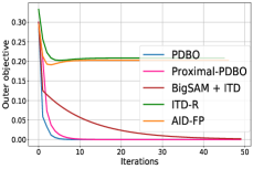
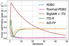
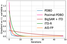
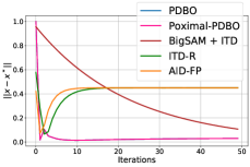
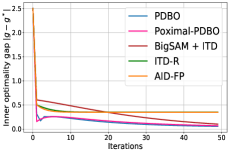
(a) outer objective v.s. iterations (b) inner opt. gap v.s. iterations (c) gradient norm v.s. iterations
Refer to caption Refer to caption Refer to caption
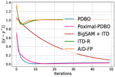
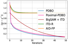
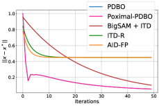
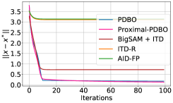
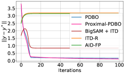
(d) yynorm𝑦superscript𝑦\|y-y^{*}\| v.s. iterations (e) xxnorm𝑥superscript𝑥\|x-x^{*}\| v.s. iterations (f) outer objective v.s. iterations
Refer to caption Refer to caption Refer to caption
(g) inner opt. gap v.s. iterations (h) yynorm𝑦superscript𝑦\|y-y^{*}\| v.s. iterations (i) xxnorm𝑥superscript𝑥\|x-x^{*}\| v.s. iterations
Refer to caption Refer to caption Refer to caption
Figure 1: Evaluation of the compared algorithms using different optimality metrics. First row and first two plots in second row: (x0,y0)=(2,(0.5,0.5))subscript𝑥0subscript𝑦020.50.5(x_{0},y_{0})=(2,(0.5,0.5)). Last plot in second row and third row: (x0,y0)=(0,(2,2))subscript𝑥0subscript𝑦0022(x_{0},y_{0})=(0,(2,2)). In both cases, PDBO is initialized with λ=2𝜆2\lambda=2.

For our PDBO, we set the learning rates τtsubscript𝜏𝑡\tau_{t}, ηtsubscript𝜂𝑡\eta_{t} to be constants 0.10.10.1, 0.20.20.2 respectively, and θt=0subscript𝜃𝑡0\theta_{t}=0. For our Proximal-PDBO, we set the τtsubscript𝜏𝑡\tau_{t}, ηtsubscript𝜂𝑡\eta_{t} and θtsubscript𝜃𝑡\theta_{t} to be the same as PDBO. Moreover, we specify T=50𝑇50T=50. For all compared methods, we fix the inner and outer learning rates to respectively 0.50.50.5 and 0.20.20.2. We use N=5𝑁5N=5 gradient descent steps to estimate the minimimal value of the smoothed inner-objective and use the same number of iterations for all compared methods.

Figure 1 shows several evaluation metrics for the algorithms under comparison over different initialization points. It can be seen that our two algorithms (Proximal-)PDBO reach the optimal solution at the fastest rate. Also as analytically proved in (Liu et al., 2020), several plots show that, with different initialization points, the classical AID and ITD methods cannot converge to the global optimal solution of the problem in eq. 10. In particular, algorithms AID-FP and ITD-R are both stuck in a bad local minima of the problem (fig. 1 (c), (d), (e), (h), and (i)). This is essentially due to the very restrictive unique minimizer assumption of these methods. When this fundamental requirement is not met, such approaches are not equipped with mechanisms to select among the multiple minimizers. Instead, our algorithm, which solves a constrained optimization problem, leverages the constraint set to guide the optimization process. In the appendix, we have provide evidence that our PDBO do converge to a KKT point of the reformulated problem in eq. 3 for the problem eq. 10.

Further Experiments. Besides the example in eq. 10, we conduct another experiment (presented in the appendix) to demonstrate that in practice PDBO can converge well for a broader class of functions even when g(x,y)𝑔𝑥𝑦g(x,y) is not convex on y𝑦y. The results show that PDBO outperforms all state-of-the-art methods with a large margin.

5.2 Hyperparameter Optimization

The goal of hyperparameter optimization (HO) is to search for the set of hyperparameters that yield the optimal value of some model selection criterion (e.g., loss on unseen data). HO can be naturally expressed as a bilevel optimization problem, in which at the inner level one searches for the model parameters that achieve the lowest training loss for given hyperparameters. At the outer level, one optimizes the hyperparameters over a validation dataset. The problem can be mathematically formulated as follows

minλ,w𝒲(λ)val(λ,w)1|𝒟val|ξ𝒟val(λ,w;ξ),with𝒲(λ)argminwtr(λ,w),formulae-sequencesubscript𝜆𝑤𝒲𝜆subscriptval𝜆𝑤1subscript𝒟valsubscript𝜉subscript𝒟val𝜆𝑤𝜉with𝒲𝜆subscriptargmin𝑤subscripttr𝜆𝑤\min_{\lambda,w\in\mathcal{W}(\lambda)}\mathcal{L}_{\mathrm{val}}(\lambda,w)\coloneqq\frac{1}{\left|\mathcal{D}_{\mathrm{val}}\right|}\sum_{\xi\in\mathcal{D}_{\mathrm{val}}}\mathcal{L}\left(\lambda,w;\xi\right),\quad\mbox{with}\quad\mathcal{W}(\lambda)\coloneqq\operatorname*{arg\,min}_{w}\mathcal{L}_{\mathrm{tr}}(\lambda,w),

where tr(λ,w):=1|𝒟tr|ζ𝒟tr((λ,w;ζ)+(λ,w))assignsubscripttr𝜆𝑤1subscript𝒟trsubscript𝜁subscript𝒟tr𝜆𝑤𝜁𝜆𝑤\mathcal{L}_{\mathrm{tr}}(\lambda,w):=\frac{1}{\left|\mathcal{D}_{\mathrm{tr}}\right|}\sum_{\zeta\in\mathcal{D}_{\mathrm{tr}}}(\mathcal{L}(\lambda,w;\zeta)+\mathcal{R}(\lambda,w)), {\mathcal{L}} is a loss function, (w,λ)𝑤𝜆\mathcal{R}(w,\lambda) is a regularizer, and 𝒟trsubscript𝒟tr{\mathcal{D}}_{\mathrm{tr}} and 𝒟valsubscript𝒟val{\mathcal{D}}_{\mathrm{val}} are respectively training and validation data.

Following (Franceschi et al., 2017; Grazzi et al., 2020a), we perform classification on the 20 Newsgroup dataset, where the classifier is modeled by an affine transformation and the cost function {\mathcal{L}} is the cross-entrpy loss. We set one 2subscript2\ell_{2}-regularization hyperparameter for each weight in w𝑤w, so that λ𝜆\lambda and w𝑤w have the same size. For our algorithm PDBO, we optimize the parameters and hyperparameters using gradient descent with a fixed learning rate of ηt1=100superscriptsubscript𝜂𝑡1100\eta_{t}^{-1}=100. We set the learning rate for the dual variable to be τt1=0.001superscriptsubscript𝜏𝑡10.001\tau_{t}^{-1}=0.001. We use N=5𝑁5N=5 gradient descent steps to estimate the minimal value of the smoothed inner-objective. For BigSAM+ITD, we set the averaging parameter to 0.50.50.5 and fix the inner and outer learning rates to be 100100100. For AID-FP and ITD-R, we use the suggested parameters in their implementations accompanying the paper (Grazzi et al., 2020a).
Refer to caption       
Algo. Acc.
PDBO 79.26
AID-FP 76.20
ITD-R 76.20
BigSAM+ITD 78.92
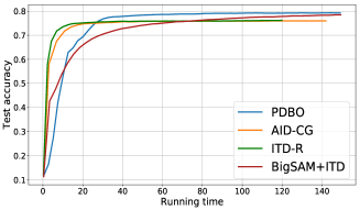
Figure 2: Classification results on 20 Newsgroup datase. Left plot: accuracy on test data v.s. running time. Right table: final best test accuracy.

The evaluations of the algorithms under comparison on a hold-out test dataset is shown in Figure 2. It can be seen that our algorithm PDBO significantly improves over AID and ITD methods, and slightly outperforms BigSAM+ITD method with a much faster convergence speed.

6 Conclusion

In this paper, we investigated a bilevel optimization problem where the inner-level function has multiple minima. Based on the reformulation of such a problem as an constrained optimization problem, we designed two algorithms PDBO and Proximal-PDBO using primal-dual gradient descent and ascent method. Specifically, PDBO features a simple design and implementation, and Proximal-PDBO features a strong convergence guarantee that we can establish. We further conducted experiments to demonstrate the desirable performance of our algorithm. As future work, it is interesting to study bilevel problems with a nonconvex inner-level function, which can have multiple inner minima. While our current design can serve as a starting point, finding a good characterization of the set of inner minima can be challenging.

References

  • Bertinetto et al. (2018) Luca Bertinetto, Joao F Henriques, Philip Torr, and Andrea Vedaldi. Meta-learning with differentiable closed-form solvers. In International Conference on Learning Representations (ICLR), 2018.
  • Boob et al. (2019) Digvijay Boob, Qi Deng, and Guanghui Lan. Stochastic first-order methods for convex and nonconvex functional constrained optimization. arXiv preprint arXiv:1908.02734, 2019.
  • Chen et al. (2021) Tianyi Chen, Yuejiao Sun, and Wotao Yin. A single-timescale stochastic bilevel optimization method. arXiv preprint arXiv:2102.04671, 2021.
  • Dempe & Zemkoho (2020) Stephan Dempe and Alain Zemkoho. Bilevel optimization. In Springer optimization and its applications. Vol. 161. Springer, 2020.
  • Domke (2012) Justin Domke. Generic methods for optimization-based modeling. In Artificial Intelligence and Statistics (AISTATS), pp. 318–326, 2012.
  • Franceschi et al. (2017) Luca Franceschi, Michele Donini, Paolo Frasconi, and Massimiliano Pontil. Forward and reverse gradient-based hyperparameter optimization. In International Conference on Machine Learning (ICML), pp. 1165–1173, 2017.
  • Franceschi et al. (2018) Luca Franceschi, Paolo Frasconi, Saverio Salzo, Riccardo Grazzi, and Massimiliano Pontil. Bilevel programming for hyperparameter optimization and meta-learning. In International Conference on Machine Learning (ICML), pp. 1568–1577, 2018.
  • Ghadimi & Wang (2018) Saeed Ghadimi and Mengdi Wang. Approximation methods for bilevel programming. arXiv preprint arXiv:1802.02246, 2018.
  • Gould et al. (2016) Stephen Gould, Basura Fernando, Anoop Cherian, Peter Anderson, Rodrigo Santa Cruz, and Edison Guo. On differentiating parameterized argmin and argmax problems with application to bi-level optimization. arXiv preprint arXiv:1607.05447, 2016.
  • Grazzi et al. (2020a) Riccardo Grazzi, Luca Franceschi, Massimiliano Pontil, and Saverio Salzo. On the iteration complexity of hypergradient computation. International Conference on Machine Learning (ICML)), 2020a.
  • Grazzi et al. (2020b) Riccardo Grazzi, Luca Franceschi, Massimiliano Pontil, and Saverio Salzo. On the iteration complexity of hypergradient computation. In Proc. International Conference on Machine Learning (ICML), 2020b.
  • Guo & Yang (2021) Zhishuai Guo and Tianbao Yang. Randomized stochastic variance-reduced methods for stochastic bilevel optimization. arXiv preprint arXiv:2105.02266, 2021.
  • Hong et al. (2020) Mingyi Hong, Hoi-To Wai, Zhaoran Wang, and Zhuoran Yang. A two-timescale framework for bilevel optimization: Complexity analysis and application to actor-critic. arXiv preprint arXiv:2007.05170, 2020.
  • Ji & Liang (2021) Kaiyi Ji and Yingbin Liang. Lower bounds and accelerated algorithms for bilevel optimization. arXiv preprint arXiv:2102.03926, 2021.
  • Ji et al. (2020) Kaiyi Ji, Jason D Lee, Yingbin Liang, and H Vincent Poor. Convergence of meta-learning with task-specific adaptation over partial parameter. In Advances in Neural Information Processing Systems (NeurIPS), 2020.
  • Ji et al. (2021) Kayi Ji, Junjie Yang, and Yingbin Liang. Bilevel optimization: Convergence analysis and enhanced design. International Conference on Machine Learning (ICML)), 2021.
  • Khanduri et al. (2021) Prashant Khanduri, Siliang Zeng, Mingyi Hong, Hoi-To Wai, Zhaoran Wang, and Zhuoran Yang. A near-optimal algorithm for stochastic bilevel optimization via double-momentum. arXiv preprint arXiv:2102.07367, 2021.
  • Konda & Tsitsiklis (2000) Vijay R Konda and John N Tsitsiklis. Actor-critic algorithms. In Advances in neural information processing systems (NeurIPS), pp.  1008–1014, 2000.
  • Lan (2020) Guanghui Lan. First-order and Stochastic Optimization Methods for Machine Learning. Springer Nature, 2020.
  • Li et al. (2020) Junyi Li, Bin Gu, and Heng Huang. Improved bilevel model: Fast and optimal algorithm with theoretical guarantee. arXiv preprint arXiv:2009.00690, 2020.
  • Liao et al. (2018) Renjie Liao, Yuwen Xiong, Ethan Fetaya, Lisa Zhang, KiJung Yoon, Xaq Pitkow, Raquel Urtasun, and Richard Zemel. Reviving and improving recurrent back-propagation. In Proc. International Conference on Machine Learning (ICML), 2018.
  • Liu et al. (2018) Hanxiao Liu, Karen Simonyan, and Yiming Yang. Darts: Differentiable architecture search. arXiv preprint arXiv:1806.09055, 2018.
  • Liu et al. (2020) Risheng Liu, Pan Mu, Xiaoming Yuan, Shangzhi Zeng, and Jin Zhang. A generic first-order algorithmic framework for bi-level programming beyond lower-level singleton. In International Conference on Machine Learning (ICML), 2020.
  • Liu et al. (2021a) Risheng Liu, Xuan Liu, Xiaoming Yuan, Shangzhi Zeng, and Jin Zhang. A value-function-based interior-point method for non-convex bi-level optimization. In International Conference on Machine Learning (ICML), 2021a.
  • Liu et al. (2021b) Risheng Liu, Yaohua Liu, Shangzhi Zeng, and Jin Zhang. Towards gradient-based bilevel optimization with non-convex followers and beyond. Advances in Neural Information Processing Systems (NeurIPS), 34, 2021b.
  • Lorraine et al. (2020) Jonathan Lorraine, Paul Vicol, and David Duvenaud. Optimizing millions of hyperparameters by implicit differentiation. In International Conference on Artificial Intelligence and Statistics (AISTATS), pp.  1540–1552. PMLR, 2020.
  • Ma et al. (2020) Runchao Ma, Qihang Lin, and Tianbao Yang. Proximally constrained methods for weakly convex optimization with weakly convex constraints. In Proc. International Conference on Machine Learning (ICML), 2020.
  • MacKay et al. (2019) Matthew MacKay, Paul Vicol, Jon Lorraine, David Duvenaud, and Roger Grosse. Self-tuning networks: Bilevel optimization of hyperparameters using structured best-response functions. arXiv preprint arXiv:1903.03088, 2019.
  • Maclaurin et al. (2015) Dougal Maclaurin, David Duvenaud, and Ryan Adams. Gradient-based hyperparameter optimization through reversible learning. In International Conference on Machine Learning (ICML), pp. 2113–2122, 2015.
  • Mangasarian & Fromovitz (1967) Olvi L Mangasarian and Stan Fromovitz. The fritz john necessary optimality conditions in the presence of equality and inequality constraints. Journal of Mathematical Analysis and applications, 17(1):37–47, 1967.
  • Nesterov et al. (2018) Yurii Nesterov et al. Lectures on convex optimization, volume 137. Springer, 2018.
  • Pedregosa (2016) Fabian Pedregosa. Hyperparameter optimization with approximate gradient. In International Conference on Machine Learning (ICML), pp. 737–746, 2016.
  • Rajeswaran et al. (2019) Aravind Rajeswaran, Chelsea Finn, Sham M Kakade, and Sergey Levine. Meta-learning with implicit gradients. In Advances in Neural Information Processing Systems (NeurIPS), pp.  113–124, 2019.
  • Sabach & Shtern (2017) Shoham Sabach and Shimrit Shtern. A first order method for solving convex bilevel optimization problems. SIAM Journal on Optimization, 27(2):640–660, 2017.
  • Shaban et al. (2019) Amirreza Shaban, Ching-An Cheng, Nathan Hatch, and Byron Boots. Truncated back-propagation for bilevel optimization. In International Conference on Artificial Intelligence and Statistics (AISTATS), pp.  1723–1732, 2019.
  • Yang et al. (2021) Junjie Yang, Kaiyi Ji, and Yingbin Liang. Provably faster algorithms for bilevel optimization. arXiv preprint arXiv:2106.04692, 2021.

Supplementary Materials

Appendix A Optimization Paths of PDBO

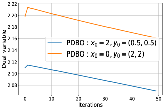
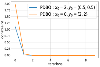
In Figure 3, we plot the optimization paths of PDBO when solving the problem in eq. 10. The two plots show that the optimization terminates with a strictly positive dual variable and that the constraint is satisfied with equality. Thus, the slackness condition is satisfied. This also confirms that our algorithm PDBO did converge to a KKT point of the reformulated problem.

(a) dual variable v.s. iterations (b) constraint v.s. iterations
Refer to caption Refer to caption
Figure 3: Optimization path of dual variable and constraint values for different initializations.

Appendix B Additional Experiment with Multiple Minima

In this section, we demonstrate that (Proximal-)PDBO is applicable to a more general class of bilevel problems in practice, where the inner problem is not necessarily convex on y𝑦y (as we require in the theoretical analysis), but still have multiple minimal points.

Consider the following bilevel optimization problem

minx𝒞,y𝒮xxa2+ya2,where𝒮xargminy𝒞sin(x+y),subscriptformulae-sequence𝑥𝒞𝑦subscript𝒮𝑥superscriptnorm𝑥𝑎2superscriptnorm𝑦𝑎2wheresubscript𝒮𝑥subscriptargmin𝑦𝒞𝑥𝑦\displaystyle\min_{x\in\mathcal{C},y\in\mathcal{S}_{x}}\|x-a\|^{2}+\|y-a\|^{2},\quad\mbox{where}\quad\mathcal{S}_{x}\coloneqq\operatorname*{arg\,min}_{y\in\mathcal{C}}\sin(x+y), (11)

where 𝒞=[10,10]𝒞1010\mathcal{C}=[-10,10], and a𝑎a is a constant (we set a=0𝑎0a=0 in our experiment).

Clearly, the problem in eq. 11 does not degenerate to single inner minimum bilevel optimization due to the sinusoid in the lower function. Such a problem is harder than the one in eq. 10, and it violates the assumption that g(x,y)𝑔𝑥𝑦g(x,y) is convex on y𝑦y.

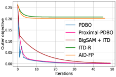
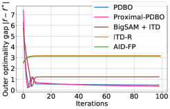
In this experiment, we compare PDBO, Proximal-PDBO, BigSAM+ITD, ITD-R and AID-FP. We initialize all methods with (x,y)=(3,3)𝑥𝑦33(x,y)=(3,3) and the hyperparameters are set to be the same as what we did in Section 5. The results are provided in Figure 4. The plots show that ITD-R and AID-FP methods converge to a bad stationary point and could not find good solutions. The methods PDBO, Proximal-PDBO, and BigSAM+ITD converge to better points but our algorithms PDBO and Proximal-PDBO significantly outperform BigSAM+ITD.

(a) outer optimality gap (b) outer convergence error (c) inner convergence error
Refer to caption Refer to caption Refer to caption
Figure 4: Comparison of different algorithms

Appendix C Calculation of h~(z)~𝑧\nabla\tilde{h}(z) in Section 2

For completeness, we provide the steps for obtaining the form of h~(z)~𝑧\nabla\tilde{h}(z) in Section 2. For the ease of reading, we restate the result here. Suppose that Assumption 1 holds. Then the gradients xh~(x,y)subscript𝑥~𝑥𝑦\nabla_{x}\tilde{h}(x,y) and yh~(x,y)subscript𝑦~𝑥𝑦\nabla_{y}\tilde{h}(x,y) of function h~(x,y)~𝑥𝑦\tilde{h}(x,y) take the following forms:

xh~(x,y)subscript𝑥~𝑥𝑦\displaystyle\nabla_{x}\tilde{h}(x,y) =xg(x,y)xg(x,y~(x)),absentsubscript𝑥𝑔𝑥𝑦subscript𝑥𝑔𝑥superscript~𝑦𝑥\displaystyle=\nabla_{x}g(x,y)-\nabla_{x}g(x,\tilde{y}^{*}(x)), (12)
yh~(x,y)subscript𝑦~𝑥𝑦\displaystyle\nabla_{y}\tilde{h}(x,y) =yg(x,y).absentsubscript𝑦𝑔𝑥𝑦\displaystyle=\nabla_{y}g(x,y). (13)
Proof.

First, eq. 13 follows immediately. Hence, we prove only eq. 12. Recall the definition of h~(x,y)~𝑥𝑦\tilde{h}(x,y):

h~(x,y)=g(x,y)g~(x)δ,~𝑥𝑦𝑔𝑥𝑦superscript~𝑔𝑥𝛿\displaystyle\tilde{h}(x,y)=g(x,y)-\tilde{g}^{*}(x)-\delta,

where g~(x)=g~(x,y~(x))superscript~𝑔𝑥~𝑔𝑥superscript~𝑦𝑥\tilde{g}^{*}(x)=\tilde{g}(x,\tilde{y}^{*}(x)) with y~(x)=argminyg~(x,y)=g(x,y)+α2y2.superscript~𝑦𝑥subscriptargmin𝑦~𝑔𝑥𝑦𝑔𝑥𝑦𝛼2superscriptnorm𝑦2\tilde{y}^{*}(x)=\operatorname*{arg\,min}_{y}\tilde{g}(x,y)=g(x,y)+\frac{\alpha}{2}\|y\|^{2}. Using the chain rule to compute the gradient with respect to x𝑥x of function h~(x,y)=g(x,y)g(x,y~(x))α2y~(x)2δ~𝑥𝑦𝑔𝑥𝑦𝑔𝑥superscript~𝑦𝑥𝛼2superscriptnormsuperscript~𝑦𝑥2𝛿\tilde{h}(x,y)=g(x,y)-g(x,\tilde{y}^{*}(x))-\frac{\alpha}{2}\|\tilde{y}^{*}(x)\|^{2}-\delta yields:

xh~(x,y)subscript𝑥~𝑥𝑦\displaystyle\nabla_{x}\tilde{h}(x,y) =xg(x,y)[xg(x,y~(x))+y~(x)xyg(x,y~(x))]αy~(x)xy~(x)absentsubscript𝑥𝑔𝑥𝑦delimited-[]subscript𝑥𝑔𝑥superscript~𝑦𝑥superscript~𝑦𝑥𝑥subscript𝑦𝑔𝑥superscript~𝑦𝑥𝛼superscript~𝑦𝑥𝑥superscript~𝑦𝑥\displaystyle=\nabla_{x}g(x,y)-\big{[}\nabla_{x}g(x,\tilde{y}^{*}(x))+\frac{\partial\tilde{y}^{*}(x)}{\partial x}\nabla_{y}g(x,\tilde{y}^{*}(x))\big{]}-\alpha\frac{\partial\tilde{y}^{*}(x)}{\partial x}\tilde{y}^{*}(x)
=xg(x,y)xg(x,y~(x))y~(x)x[yg(x,y~(x))+αy~(x)].absentsubscript𝑥𝑔𝑥𝑦subscript𝑥𝑔𝑥superscript~𝑦𝑥superscript~𝑦𝑥𝑥delimited-[]subscript𝑦𝑔𝑥superscript~𝑦𝑥𝛼superscript~𝑦𝑥\displaystyle=\nabla_{x}g(x,y)-\nabla_{x}g(x,\tilde{y}^{*}(x))-\frac{\partial\tilde{y}^{*}(x)}{\partial x}\big{[}\nabla_{y}g(x,\tilde{y}^{*}(x))+\alpha\tilde{y}^{*}(x)\big{]}.

The first order optimality condition ensures that yg(x,y~(x))+αy~(x)=0subscript𝑦𝑔𝑥superscript~𝑦𝑥𝛼superscript~𝑦𝑥0\nabla_{y}g(x,\tilde{y}^{*}(x))+\alpha\tilde{y}^{*}(x)=0. Hence, we obain the desired result:

xh~(x,y)subscript𝑥~𝑥𝑦\displaystyle\nabla_{x}\tilde{h}(x,y) =xg(x,y)xg(x,y~(x)).absentsubscript𝑥𝑔𝑥𝑦subscript𝑥𝑔𝑥superscript~𝑦𝑥\displaystyle=\nabla_{x}g(x,y)-\nabla_{x}g(x,\tilde{y}^{*}(x)).

Appendix D Proof of Theorem 1

D.1 Supporting Lemmas

We first cite two standard lemmas, which are useful for our proof here.

Lemma 2 (Lemma 3.5 Lan (2020)).

Suppose that 𝒮𝒮\mathcal{S} is a convex and closed subset of nsuperscript𝑛\mathbb{R}^{n}, x𝒮𝑥𝒮x\in\mathcal{S}, and vn𝑣superscript𝑛v\in\mathbb{R}^{n}. Define x¯=Π𝒮(xv)¯𝑥subscriptΠ𝒮𝑥𝑣\bar{x}=\Pi_{\mathcal{S}}\left(x-v\right). Then, for any x~𝒮~𝑥𝒮\tilde{x}\in\mathcal{S}, the following inequality holds:

x,v+12x¯x~22+12xx¯2212xx~22.𝑥𝑣12superscriptsubscriptnorm¯𝑥~𝑥2212superscriptsubscriptnorm𝑥¯𝑥2212superscriptsubscriptnorm𝑥~𝑥22\displaystyle\langle x,v\rangle+\tfrac{1}{2}\|\bar{x}-\tilde{x}\|_{2}^{2}+\tfrac{1}{2}\|x-\bar{x}\|_{2}^{2}\leq\tfrac{1}{2}\|x-\tilde{x}\|_{2}^{2}.
Lemma 3 (Theorem 2.2.14 Nesterov et al. (2018)).

Suppose that Assumption 1 holds. Consider the projected gradient descent in eq. 5. Define y~(xt)argminy𝒴g(xt,y)+α2y22superscript~𝑦subscript𝑥𝑡subscriptargmin𝑦𝒴𝑔subscript𝑥𝑡𝑦𝛼2superscriptsubscriptnorm𝑦22\tilde{y}^{*}(x_{t})\coloneqq\operatorname*{arg\,min}_{y\in\mathcal{Y}}g(x_{t},y)+\tfrac{\alpha}{2}\|y\|_{2}^{2}. We have

y^(xt)y~(xt)2=y^Ny~(xt)2(1αρg+2α)Ny^0y~(xt)2.subscriptnormsuperscript^𝑦subscript𝑥𝑡superscript~𝑦subscript𝑥𝑡2subscriptnormsubscript^𝑦𝑁superscript~𝑦subscript𝑥𝑡2superscript1𝛼subscript𝜌𝑔2𝛼𝑁subscriptnormsubscript^𝑦0superscript~𝑦subscript𝑥𝑡2\displaystyle\|\hat{y}^{*}(x_{t})-\tilde{y}^{*}(x_{t})\|_{2}=\|\hat{y}_{N}-\tilde{y}^{*}(x_{t})\|_{2}\leq\left(1-\tfrac{\alpha}{\rho_{g}+2\alpha}\right)^{N}\|\hat{y}_{0}-\tilde{y}^{*}(x_{t})\|_{2}.

Next, we establish an upper bound on the optimal dual variable in the following lemma.

Lemma 4.

Suppose that Assumptions 1 and 2 hold. Then, there exists λsuperscript𝜆\lambda^{*} satisfying 0λDfδ0superscript𝜆subscript𝐷𝑓𝛿0\leq\lambda^{*}\leq\tfrac{D_{f}}{\delta}, where Df=supz,z𝒵|f(z)f(z)|subscript𝐷𝑓subscriptsupremum𝑧superscript𝑧𝒵𝑓𝑧𝑓superscript𝑧D_{f}=\sup_{z,z^{\prime}\in\mathcal{Z}}|f(z)-f(z^{\prime})|, so that for z:=argminz𝒵f(z)+λh~(z)assignsuperscript𝑧subscriptargmin𝑧𝒵𝑓𝑧superscript𝜆~𝑧z^{*}:=\text{argmin}_{z\in\mathcal{Z}}f(z)+\lambda^{*}\tilde{h}(z), h~(z)0~superscript𝑧0\tilde{h}(z^{*})\leq 0, and the KKT condition holds, i.e., λh~(z)=0superscript𝜆~superscript𝑧0\lambda^{*}\tilde{h}(z^{*})=0, and f(z)+λh~(z)𝒩𝒵(z)𝑓superscript𝑧superscript𝜆~superscript𝑧subscript𝒩𝒵superscript𝑧\nabla f(z^{*})+\lambda^{*}\nabla\tilde{h}(z^{*})\in-\mathcal{N}_{\mathcal{Z}}(z^{*}), where 𝒩𝒵(z)subscript𝒩𝒵superscript𝑧\mathcal{N}_{\mathcal{Z}}(z^{*}) is the normal cone defined as 𝒩𝒵(z)={vp+d:v,zz0, for all z𝒵}subscript𝒩𝒵superscript𝑧conditional-set𝑣superscript𝑝𝑑formulae-sequence𝑣𝑧superscript𝑧0 for all 𝑧𝒵\mathcal{N}_{\mathcal{Z}}(z^{*})=\{v\in\mathbb{R}^{p+d}:\langle v,z-z^{*}\rangle\leq 0,\mbox{ for all }z\in\mathcal{Z}\}.

Proof.

Pick any x0𝒳subscript𝑥0𝒳x_{0}\in\mathcal{X}. Let y0=argminy𝒴g(x,y)+α2y22subscript𝑦0subscriptargmin𝑦𝒴𝑔𝑥𝑦𝛼2superscriptsubscriptnorm𝑦22y_{0}=\operatorname*{arg\,min}_{y\in\mathcal{Y}}g(x,y)+\tfrac{\alpha}{2}\|y\|_{2}^{2}, and z0=(x0,y0)subscript𝑧0subscript𝑥0subscript𝑦0z_{0}=(x_{0},y_{0}). Then, h~(z0)=g(x0,y0)g~(x0)δ=δ~subscript𝑧0𝑔subscript𝑥0subscript𝑦0superscript~𝑔subscript𝑥0𝛿𝛿\tilde{h}(z_{0})=g(x_{0},y_{0})-\tilde{g}^{*}(x_{0})-\delta=-\delta holds, which implies that z0subscript𝑧0z_{0} is a strictly feasible point. The existence of such a strictly feasible point z0subscript𝑧0z_{0} ensures that the Slater’s condition holds, and then the standard result (see, e.g., Lan (2020)) implies the existence of λ0superscript𝜆0\lambda^{*}\geq 0 that satisfies for z:=argminz𝒵f(z)+λh~(z)assignsuperscript𝑧subscriptargmin𝑧𝒵𝑓𝑧superscript𝜆~𝑧z^{*}:=\text{argmin}_{z\in\mathcal{Z}}f(z)+\lambda^{*}\tilde{h}(z), h~(z)0~superscript𝑧0\tilde{h}(z^{*})\leq 0, λh~(z)=0superscript𝜆~superscript𝑧0\lambda^{*}\tilde{h}(z^{*})=0, and f(z)+λh~(z)𝒩𝒵(z)𝑓superscript𝑧superscript𝜆~superscript𝑧subscript𝒩𝒵superscript𝑧\nabla f(z^{*})+\lambda^{*}\nabla\tilde{h}(z^{*})\in-\mathcal{N}_{\mathcal{Z}}(z^{*}).

Define the dual function as d(λ):=minz𝒵(z,λ)assign𝑑𝜆subscript𝑧𝒵𝑧𝜆d(\lambda):=\min_{z\in\mathcal{Z}}\mathcal{L}(z,\lambda). Then, we have, for any λ𝜆\lambda and z𝒵𝑧𝒵z\in\mathcal{Z},

d(λ)f(z0)+λh^(z0)=f(z0)δλ.𝑑𝜆𝑓subscript𝑧0𝜆^subscript𝑧0𝑓subscript𝑧0𝛿𝜆\displaystyle d(\lambda)\leq f(z_{0})+\lambda\hat{h}(z_{0})=f(z_{0})-\delta\lambda. (14)

Taking λ=λ𝜆superscript𝜆\lambda=\lambda^{*} in eq. 14 and using the fact that |d(λ)f(z0)|=|f(z)f(z0)|Df𝑑superscript𝜆𝑓subscript𝑧0𝑓superscript𝑧𝑓subscript𝑧0subscript𝐷𝑓|d(\lambda^{*})-f(z_{0})|=|f(z^{*})-f(z_{0})|\leq D_{f}, where Df=supz,z𝒵|f(z)f(z)|subscript𝐷𝑓subscriptsupremum𝑧superscript𝑧𝒵𝑓𝑧𝑓superscript𝑧D_{f}=\sup_{z,z^{\prime}\in\mathcal{Z}}|f(z)-f(z^{\prime})|, we complete the proof. ∎

In the next lemma, we show that the constrained function h~(z)~𝑧\tilde{h}(z) is gradient Lipschitz continuous.

Lemma 5.

Suppose that Assumption 1 holds. Then, the gradient h~(z)=(xh~(x,y),yh~(x,y))~𝑧superscriptsubscript𝑥~𝑥𝑦subscript𝑦~𝑥𝑦top\nabla\tilde{h}(z)=\big{(}\nabla_{x}\tilde{h}(x,y),\nabla_{y}\tilde{h}(x,y)\big{)}^{\top} is Lipschitz continuous with constant ρh=ρg(2+ρg/α)subscript𝜌subscript𝜌𝑔2subscript𝜌𝑔𝛼\rho_{h}=\rho_{g}(2+\rho_{g}/\alpha).

Proof.

Recall the form of h~(z)~𝑧\nabla\tilde{h}(z) is given by

h~(z)=~𝑧absent\displaystyle\nabla\tilde{h}(z)= (xg(x,y)yg(x,y))(xg(x,y~(x))𝟎d)=g(z)(GxGy),subscript𝑥𝑔𝑥𝑦subscript𝑦𝑔𝑥𝑦subscript𝑥𝑔𝑥superscript~𝑦𝑥subscript0𝑑𝑔𝑧subscript𝐺𝑥subscript𝐺𝑦\displaystyle\left(\begin{array}[]{c}\nabla_{x}g(x,y)\\ \nabla_{y}g(x,y)\end{array}\right)-\left(\begin{array}[]{c}\nabla_{x}g(x,\tilde{y}^{*}(x))\\ \mathbf{0}_{d}\end{array}\right)=\nabla g(z)-\left(\begin{array}[]{c}G_{x}\\ G_{y}\end{array}\right), (21)

where Gx:=xg(x,y~(x))assignsubscript𝐺𝑥subscript𝑥𝑔𝑥superscript~𝑦𝑥G_{x}:=\nabla_{x}g(x,\tilde{y}^{*}(x)) and Gy:=𝟎ddassignsubscript𝐺𝑦subscript0𝑑superscript𝑑G_{y}:=\mathbf{0}_{d}\in\mathbb{R}^{d} is a vector of all zeros. Taking derivative w.r.t. z𝑧z yields:

2h~(z)=superscript2~𝑧absent\displaystyle\nabla^{2}\tilde{h}(z)= 2g(z)(GxxGxyGyxGyy)superscript2𝑔𝑧subscript𝐺𝑥𝑥subscript𝐺𝑥𝑦subscript𝐺𝑦𝑥subscript𝐺𝑦𝑦\displaystyle\nabla^{2}g(z)-\left(\begin{array}[]{cc}\frac{\partial G_{x}}{\partial x}&\frac{\partial G_{x}}{\partial y}\\ \frac{\partial G_{y}}{\partial x}&\frac{\partial G_{y}}{\partial y}\end{array}\right) (24)
=\displaystyle= 2g(z)(xg(x,y~(x))x𝟎p×d𝟎d×p𝟎d×d)M.superscript2𝑔𝑧subscriptsubscript𝑥𝑔𝑥superscript~𝑦𝑥𝑥subscript0𝑝𝑑subscript0𝑑𝑝subscript0𝑑𝑑𝑀\displaystyle\nabla^{2}g(z)-\underbrace{\left(\begin{array}[]{cc}\frac{\partial\nabla_{x}g(x,\tilde{y}^{*}(x))}{\partial x}&\mathbf{0}_{p\times d}\\ \mathbf{0}_{d\times p}&\mathbf{0}_{d\times d}\end{array}\right)}_{M}. (27)

where 𝟎m×nm×nsubscript0𝑚𝑛superscript𝑚𝑛\mathbf{0}_{m\times n}\in\mathbb{R}^{m\times n} is a matrix of all zeros.

Recall that in Assumption 1, we assume g(z)g(z)2ρgzz2subscriptnorm𝑔𝑧𝑔superscript𝑧2subscript𝜌𝑔subscriptnorm𝑧superscript𝑧2\|\nabla g(z)-\nabla g(z^{\prime})\|_{2}\leq\rho_{g}\|z-z^{\prime}\|_{2} for all z,z𝒵𝑧superscript𝑧𝒵z,z^{\prime}\in\mathcal{Z}, which immediately implies 2g(z)2ρgsubscriptnormsuperscript2𝑔𝑧2subscript𝜌𝑔\|\nabla^{2}g(z)\|_{2}\leq\rho_{g}. Note that in the sequel, 2\|\cdot\|_{2} of a matrix denotes the spectral norm. Moreover, let

2g(z)=(xx2g(z)xy2g(z)yx2g(z)yy2g(z)).superscript2𝑔𝑧matrixsubscriptsuperscript2𝑥𝑥𝑔𝑧subscriptsuperscript2𝑥𝑦𝑔𝑧subscriptsuperscript2𝑦𝑥𝑔𝑧subscriptsuperscript2𝑦𝑦𝑔𝑧\nabla^{2}g(z)=\begin{pmatrix}\nabla^{2}_{xx}g(z)&\nabla^{2}_{xy}g(z)\\ \nabla^{2}_{yx}g(z)&\nabla^{2}_{yy}g(z)\end{pmatrix}.

Given any xp𝑥superscript𝑝x\in\mathbb{R}^{p}, we have 2g(z)(x0)=(xx2g(z)xyx2g(z)x)superscript2𝑔𝑧matrix𝑥0matrixsubscriptsuperscript2𝑥𝑥𝑔𝑧𝑥subscriptsuperscript2𝑦𝑥𝑔𝑧𝑥\nabla^{2}g(z)\begin{pmatrix}x\\ 0\end{pmatrix}=\begin{pmatrix}\nabla^{2}_{xx}g(z)x\\ \nabla^{2}_{yx}g(z)x\end{pmatrix}. Thus, the following inequality holds

xx2g(z)x2(xx2g(z)xyx2g(z)x)2=2g(z)(x0)22g(z)2x2ρgx2.subscriptnormsubscriptsuperscript2𝑥𝑥𝑔𝑧𝑥2subscriptnormmatrixsubscriptsuperscript2𝑥𝑥𝑔𝑧𝑥subscriptsuperscript2𝑦𝑥𝑔𝑧𝑥2subscriptnormsuperscript2𝑔𝑧matrix𝑥02subscriptnormsuperscript2𝑔𝑧2subscriptnorm𝑥2subscript𝜌𝑔subscriptnorm𝑥2\displaystyle\|\nabla^{2}_{xx}g(z)x\|_{2}\leq\left\|\begin{pmatrix}\nabla^{2}_{xx}g(z)x\\ \nabla^{2}_{yx}g(z)x\end{pmatrix}\right\|_{2}=\left\|\nabla^{2}g(z)\begin{pmatrix}x\\ 0\end{pmatrix}\right\|_{2}\leq\|\nabla^{2}g(z)\|_{2}\|x\|_{2}\leq\rho_{g}\|x\|_{2}. (28)

Following the definition of the spectral norm of xx2g(z)superscriptsubscript𝑥𝑥2𝑔𝑧\nabla_{xx}^{2}g(z), we have

xx2g(z)2ρg.subscriptnormsuperscriptsubscript𝑥𝑥2𝑔𝑧2subscript𝜌𝑔\|\nabla_{xx}^{2}g(z)\|_{2}\leq\rho_{g}. (29)

Following the similar steps to eq. 28, we have

yx2g(z)2ρg.subscriptnormsuperscriptsubscript𝑦𝑥2𝑔𝑧2subscript𝜌𝑔\|\nabla_{yx}^{2}g(z)\|_{2}\leq\rho_{g}. (30)

We next upper-bound the spectral norm of the matrix M𝑀M defined in eq. 27. We have:

2g~(z)2=M2subscriptnormsuperscript2superscript~𝑔𝑧2subscriptnorm𝑀2\displaystyle\|\nabla^{2}\tilde{g}^{*}(z)\|_{2}=\left\|M\right\|_{2} =(xg(x,y~(x))x𝟎p×d𝟎d×p𝟎d×d)2xg(x,y~(x))x2,absentsubscriptnormsubscript𝑥𝑔𝑥superscript~𝑦𝑥𝑥subscript0𝑝𝑑subscript0𝑑𝑝subscript0𝑑𝑑2subscriptnormsubscript𝑥𝑔𝑥superscript~𝑦𝑥𝑥2\displaystyle=\left\|\left(\begin{array}[]{cc}\frac{\partial\nabla_{x}g(x,\tilde{y}^{*}(x))}{\partial x}&\mathbf{0}_{p\times d}\\ \mathbf{0}_{d\times p}&\mathbf{0}_{d\times d}\end{array}\right)\right\|_{2}\leq\left\|\frac{\partial\nabla_{x}g(x,\tilde{y}^{*}(x))}{\partial x}\right\|_{2}, (33)

where eq. 33 follows from the fact that for the block matrix C=(A𝟎𝟎B)𝐶𝐴00𝐵C=\left(\begin{array}[]{cc}A&\mathbf{0}\\ \mathbf{0}&B\end{array}\right), we have C2max{A2,B2}subscriptnorm𝐶2subscriptnorm𝐴2subscriptnorm𝐵2\big{\|}C\big{\|}_{2}\leq\max\big{\{}\big{\|}A\big{\|}_{2},\big{\|}B\big{\|}_{2}\big{\}}. Further, using the chain rule, we obtain

xg(x,y~(x))x=x2g(x,y~(x))+y~(x)xyxg(x,y~(x)).subscript𝑥𝑔𝑥superscript~𝑦𝑥𝑥superscriptsubscript𝑥2𝑔𝑥superscript~𝑦𝑥superscript~𝑦𝑥𝑥subscript𝑦subscript𝑥𝑔𝑥superscript~𝑦𝑥\displaystyle\frac{\partial\nabla_{x}g(x,\tilde{y}^{*}(x))}{\partial x}=\nabla_{x}^{2}g(x,\tilde{y}^{*}(x))+\frac{\partial\tilde{y}^{*}(x)}{\partial x}\nabla_{y}\nabla_{x}g(x,\tilde{y}^{*}(x)). (34)

Thus, taking the norm on both sides of the above equation and applying the triangle inequality yield

xg(x,y~(x))x2subscriptnormsubscript𝑥𝑔𝑥superscript~𝑦𝑥𝑥2\displaystyle\Big{\|}\frac{\partial\nabla_{x}g(x,\tilde{y}^{*}(x))}{\partial x}\Big{\|}_{2} xx2g(x,y~(x))2+y~(x)x2yxg(x,y~(x))2absentsubscriptnormsuperscriptsubscript𝑥𝑥2𝑔𝑥superscript~𝑦𝑥2subscriptnormsuperscript~𝑦𝑥𝑥2subscriptnormsubscript𝑦subscript𝑥𝑔𝑥superscript~𝑦𝑥2\displaystyle\leq\Big{\|}\nabla_{xx}^{2}g(x,\tilde{y}^{*}(x))\Big{\|}_{2}+\Big{\|}\frac{\partial\tilde{y}^{*}(x)}{\partial x}\Big{\|}_{2}\Big{\|}\nabla_{y}\nabla_{x}g(x,\tilde{y}^{*}(x))\Big{\|}_{2}
(i)ρg+ρgy~(x)x2,𝑖subscript𝜌𝑔subscript𝜌𝑔subscriptnormsuperscript~𝑦𝑥𝑥2\displaystyle\overset{(i)}{\leq}\rho_{g}+\rho_{g}\left\|\frac{\partial\tilde{y}^{*}(x)}{\partial x}\right\|_{2}, (35)

where (i)𝑖(i) follows from eqs. 29 and 30.

Applying implicit differentiation w.r.t. x𝑥x to the optimality condition of y~(x)superscript~𝑦𝑥\tilde{y}^{*}(x) implies yg(x,y~(x))+αy~(x)=0subscript𝑦𝑔𝑥superscript~𝑦𝑥𝛼superscript~𝑦𝑥0\nabla_{y}g(x,\tilde{y}^{*}(x))+\alpha\tilde{y}^{*}(x)=0. This yields

xyg(x,y~(x))+y~(x)xy2g(x,y~(x))+αy~(x)x=0,subscript𝑥subscript𝑦𝑔𝑥superscript~𝑦𝑥superscript~𝑦𝑥𝑥superscriptsubscript𝑦2𝑔𝑥superscript~𝑦𝑥𝛼superscript~𝑦𝑥𝑥0\displaystyle\nabla_{x}\nabla_{y}g(x,\tilde{y}^{*}(x))+\frac{\partial\tilde{y}^{*}(x)}{\partial x}\nabla_{y}^{2}g(x,\tilde{y}^{*}(x))+\alpha\frac{\partial\tilde{y}^{*}(x)}{\partial x}=0,

which further yields

y~(x)x=[y2g(x,y~(x))+α𝐈]1xyg(x,y~(x)).superscript~𝑦𝑥𝑥superscriptdelimited-[]superscriptsubscript𝑦2𝑔𝑥superscript~𝑦𝑥𝛼𝐈1subscript𝑥subscript𝑦𝑔𝑥superscript~𝑦𝑥\displaystyle\frac{\partial\tilde{y}^{*}(x)}{\partial x}=-\Big{[}\nabla_{y}^{2}g(x,\tilde{y}^{*}(x))+\alpha\mathbf{I}\Big{]}^{-1}\nabla_{x}\nabla_{y}g(x,\tilde{y}^{*}(x)).

Hence, we obtain

y~(x)x2subscriptnormsuperscript~𝑦𝑥𝑥2absent\displaystyle\Big{\|}\frac{\partial\tilde{y}^{*}(x)}{\partial x}\Big{\|}_{2}\leq [y2g(x,y~(x))+α𝐈]12xyg(x,y~(x))2ρgα,subscriptnormsuperscriptdelimited-[]superscriptsubscript𝑦2𝑔𝑥superscript~𝑦𝑥𝛼𝐈12subscriptnormsubscript𝑥subscript𝑦𝑔𝑥superscript~𝑦𝑥2subscript𝜌𝑔𝛼\displaystyle\Big{\|}\Big{[}\nabla_{y}^{2}g(x,\tilde{y}^{*}(x))+\alpha\mathbf{I}\Big{]}^{-1}\Big{\|}_{2}\Big{\|}\nabla_{x}\nabla_{y}g(x,\tilde{y}^{*}(x))\Big{\|}_{2}\leq\frac{\rho_{g}}{\alpha}, (36)

where the last inequality follows from Assumption 1. Hence, combining eq. 33, eq. 35, and eq. 36, we have

2g~(z)2=M2ρg+ρgρgα,subscriptnormsuperscript2superscript~𝑔𝑧2subscriptnorm𝑀2subscript𝜌𝑔subscript𝜌𝑔subscript𝜌𝑔𝛼\displaystyle\|\nabla^{2}\tilde{g}^{*}(z)\|_{2}=\big{\|}M\big{\|}_{2}\leq\rho_{g}+\rho_{g}\frac{\rho_{g}}{\alpha}, (37)

which, in conjunction of eq. 27, yields

2h~(z)22g(z)2+M2ρg+ρg+ρg2α=ρg(2+ρgα).subscriptnormsuperscript2~𝑧2subscriptnormsuperscript2𝑔𝑧2subscriptnorm𝑀2subscript𝜌𝑔subscript𝜌𝑔superscriptsubscript𝜌𝑔2𝛼subscript𝜌𝑔2subscript𝜌𝑔𝛼\displaystyle\big{\|}\nabla^{2}\tilde{h}(z)\big{\|}_{2}\leq\big{\|}\nabla^{2}g(z)\big{\|}_{2}+\big{\|}M\big{\|}_{2}\leq\rho_{g}+\rho_{g}+\frac{\rho_{g}^{2}}{\alpha}=\rho_{g}\left(2+\frac{\rho_{g}}{\alpha}\right).

This completes the proof. ∎

D.2 Proof of Theorem 1

Based on the above lemmas, we develop the proof of Theorem 1. We first formally restate the theorem with the full details.

Theorem 3 (Formal Statement of Theorem 1).

Suppose Assumption 1 holds. Let γt=t+t0+1subscript𝛾𝑡𝑡subscript𝑡01\gamma_{t}=t+t_{0}+1, ηt=μ(t+t0+1)2subscript𝜂𝑡𝜇𝑡subscript𝑡012\eta_{t}=\frac{\mu(t+t_{0}+1)}{2}, τt=4Lg2μtsubscript𝜏𝑡4superscriptsubscript𝐿𝑔2𝜇𝑡\tau_{t}=\frac{4L_{g}^{2}}{\mu t}, θt=t+t0t+t0+1subscript𝜃𝑡𝑡subscript𝑡0𝑡subscript𝑡01\theta_{t}=\frac{t+t_{0}}{t+t_{0}+1}, where Lg=supzzg(z)2subscript𝐿𝑔subscriptsupremum𝑧subscriptnormsubscript𝑧𝑔𝑧2L_{g}=\sup_{z}\|\nabla_{z}g(z)\|_{2}, t0=2(ρf+Bρh)μsubscript𝑡02subscript𝜌𝑓𝐵subscript𝜌𝜇t_{0}=\frac{2(\rho_{f}+B\rho_{h})}{\mu}, B=Dfδ+1𝐵subscript𝐷𝑓𝛿1B=\tfrac{D_{f}}{\delta}+1, where Df=supz,z𝒵|f(z)f(z)|subscript𝐷𝑓subscriptsupremum𝑧superscript𝑧𝒵𝑓𝑧𝑓superscript𝑧D_{f}=\sup_{z,z^{\prime}\in\mathcal{Z}}|f(z)-f(z^{\prime})|, and ρhsubscript𝜌\rho_{h} is given in Lemma 5. Then, we have

f(z¯)f(z)𝑓¯𝑧𝑓superscript𝑧\displaystyle f(\bar{z})-f(z^{*}) 2LgBD𝒵T2+γ0(η0μ)zz022T2+(ρgD𝒵+4Lg)BD𝒵(1αρg+2α)N,absent2subscript𝐿𝑔𝐵subscript𝐷𝒵superscript𝑇2subscript𝛾0subscript𝜂0𝜇superscriptsubscriptnormsuperscript𝑧subscript𝑧022superscript𝑇2subscript𝜌𝑔subscript𝐷𝒵4subscript𝐿𝑔𝐵subscript𝐷𝒵superscript1𝛼subscript𝜌𝑔2𝛼𝑁\displaystyle\leq\frac{2L_{g}BD_{\mathcal{Z}}}{T^{2}}+\frac{\gamma_{0}(\eta_{0}-\mu)\|{z}^{*}-z_{0}\|_{2}^{2}}{T^{2}}+(\rho_{g}D_{\mathcal{Z}}+4L_{g})BD_{\mathcal{Z}}\left(1-\tfrac{\alpha}{\rho_{g}+2\alpha}\right)^{N},
[h~(z¯)]+2LgBD𝒵+γ0τ0B2+γ0(η0μ)D𝒵2T2+(ρgD𝒵+4Lg)BD𝒵(1αρg+2α)N,subscriptdelimited-[]~¯𝑧2subscript𝐿𝑔𝐵subscript𝐷𝒵subscript𝛾0subscript𝜏0superscript𝐵2subscript𝛾0subscript𝜂0𝜇superscriptsubscript𝐷𝒵2superscript𝑇2subscript𝜌𝑔subscript𝐷𝒵4subscript𝐿𝑔𝐵subscript𝐷𝒵superscript1𝛼subscript𝜌𝑔2𝛼𝑁\displaystyle[\tilde{h}(\bar{z})]_{+}\leq\frac{2L_{g}BD_{\mathcal{Z}}+\gamma_{0}\tau_{0}B^{2}+\gamma_{0}(\eta_{0}-\mu){D}_{\mathcal{Z}}^{2}}{T^{2}}+(\rho_{g}D_{\mathcal{Z}}+4L_{g})BD_{\mathcal{Z}}\left(1-\tfrac{\alpha}{\rho_{g}+2\alpha}\right)^{N},

and

z¯z222γ0τ0B2+2γ0(η0μ)D𝒵2μT2+2(T+t0+1)2T2(ρgD𝒵+4Lg)BD𝒵(1αρg+2α)N,superscriptsubscriptnorm¯𝑧superscript𝑧222subscript𝛾0subscript𝜏0superscript𝐵22subscript𝛾0subscript𝜂0𝜇superscriptsubscript𝐷𝒵2𝜇superscript𝑇22superscript𝑇subscript𝑡012superscript𝑇2subscript𝜌𝑔subscript𝐷𝒵4subscript𝐿𝑔𝐵subscript𝐷𝒵superscript1𝛼subscript𝜌𝑔2𝛼𝑁\displaystyle\|\bar{z}-z^{*}\|_{2}^{2}\leq\frac{2{\gamma_{0}\tau_{0}}B^{2}+2{\gamma_{0}(\eta_{0}-\mu)}D_{\mathcal{Z}}^{2}}{\mu T^{2}}+\frac{2(T+t_{0}+1)^{2}}{T^{2}}(\rho_{g}D_{\mathcal{Z}}+4L_{g})BD_{\mathcal{Z}}\left(1-\tfrac{\alpha}{\rho_{g}+2\alpha}\right)^{N},

where z=argminz𝒵{f(z):h~(z)0}superscript𝑧subscriptargmin𝑧𝒵:𝑓𝑧~𝑧0z^{*}=\operatorname*{arg\,min}_{z\in\mathcal{Z}}\{f(z):\tilde{h}(z)\leq 0\}.

Proof.

We first define some notations that will be used later. Let d^t=(1+θt)h^(zt)θth^(zt1)subscript^𝑑𝑡1subscript𝜃𝑡^subscript𝑧𝑡subscript𝜃𝑡^subscript𝑧𝑡1\hat{d}_{t}=(1+\theta_{t})\hat{h}(z_{t})-\theta_{t}\hat{h}(z_{t-1}), dt=(1+θt)h~(zt)θth~(zt1)subscript𝑑𝑡1subscript𝜃𝑡~subscript𝑧𝑡subscript𝜃𝑡~subscript𝑧𝑡1{d}_{t}=(1+\theta_{t})\tilde{h}(z_{t})-\theta_{t}\tilde{h}(z_{t-1}), and ξt=h^(zt)h^(zt1)subscript𝜉𝑡^subscript𝑧𝑡^subscript𝑧𝑡1\xi_{t}=\hat{h}(z_{t})-\hat{h}(z_{t-1}). Furthermore, we define the primal-dual gap function as

Q(w,w~)f(z)+λ~h~(z)(f(z~)+λh~(z~)),𝑄𝑤~𝑤𝑓𝑧~𝜆~𝑧𝑓~𝑧𝜆~~𝑧\displaystyle Q(w,\tilde{w})\coloneqq f(z)+\tilde{\lambda}\tilde{h}(z)-\left(f(\tilde{z})+\lambda\tilde{h}(\tilde{z})\right),

where w=(z,λ)𝑤𝑧𝜆w=(z,\lambda), w~=(z~,λ~)𝒵×Λ~𝑤~𝑧~𝜆𝒵Λ\tilde{w}=(\tilde{z},\tilde{\lambda})\in\mathcal{Z}\times{\Lambda} are primal-dual pairs.

Consider the update of λ𝜆\lambda in eq. 6. Applying Lemma 2 with v=d^t/τt𝑣subscript^𝑑𝑡subscript𝜏𝑡v=-{\hat{d}_{t}}/{\tau_{t}}, 𝒮=Λ𝒮Λ\mathcal{S}=\Lambda, x¯=λt+1¯𝑥subscript𝜆𝑡1\bar{x}=\lambda_{t+1}, x=λt𝑥subscript𝜆𝑡x=\lambda_{t} and letting x~=λ~𝑥𝜆\tilde{x}=\lambda be an arbitrary point inside ΛΛ\Lambda, we have

(λt+1λ)d^tτt2((λλt)2(λt+1λt)2(λλt+1)2).subscript𝜆𝑡1𝜆subscript^𝑑𝑡subscript𝜏𝑡2superscript𝜆subscript𝜆𝑡2superscriptsubscript𝜆𝑡1subscript𝜆𝑡2superscript𝜆subscript𝜆𝑡12\displaystyle-(\lambda_{t+1}-\lambda)\hat{d}_{t}\leq\frac{\tau_{t}}{2}\left((\lambda-\lambda_{t})^{2}-(\lambda_{t+1}-\lambda_{t})^{2}-(\lambda-\lambda_{t+1})^{2}\right). (38)

Similarly, consider the update of z𝑧z in eq. 7. Applying Lemma 2 with

v=1ηt(f(zt)+λt+1^h~(zt))1ηt^(zt,λt+1),𝑣1subscript𝜂𝑡𝑓subscript𝑧𝑡subscript𝜆𝑡1^~subscript𝑧𝑡1subscript𝜂𝑡^subscript𝑧𝑡subscript𝜆𝑡1v=\tfrac{1}{\eta_{t}}\left(\nabla f(z_{t})+\lambda_{t+1}\hat{\nabla}\tilde{h}(z_{t})\right)\coloneqq\tfrac{1}{\eta_{t}}\hat{\nabla}\mathcal{L}(z_{t},\lambda_{t+1}),

𝒮=𝒵𝒮𝒵\mathcal{S}=\mathcal{Z}, x¯=zt+1¯𝑥subscript𝑧𝑡1\bar{x}=z_{t+1}, x=zt𝑥subscript𝑧𝑡x=z_{t} and let x~=z~𝑥𝑧\tilde{x}=z be an arbitrary point inside 𝒵𝒵\mathcal{Z}, we obtain

^z(zt,λt+1),zt+1zηt2((zzt)2(zt+1zt)2(zzt+1)2).subscript^𝑧subscript𝑧𝑡subscript𝜆𝑡1subscript𝑧𝑡1𝑧subscript𝜂𝑡2superscript𝑧subscript𝑧𝑡2superscriptsubscript𝑧𝑡1subscript𝑧𝑡2superscript𝑧subscript𝑧𝑡12\displaystyle\langle\hat{\nabla}_{z}\mathcal{L}(z_{t},\lambda_{t+1}),z_{t+1}-z\rangle\leq\frac{\eta_{t}}{2}\left((z-z_{t})^{2}-(z_{t+1}-z_{t})^{2}-(z-z_{t+1})^{2}\right). (39)

Recall that f(z)𝑓𝑧f(z) and h~(z)~𝑧\tilde{h}(z) are ρfsubscript𝜌𝑓\rho_{f}- and ρhsubscript𝜌\rho_{h}-gradient Lipschitz (see Assumption 1 and Lemma 5). This implies

f(zt),zt+1ztf(zt+1)f(zt)ρfztzt+1222,𝑓subscript𝑧𝑡subscript𝑧𝑡1subscript𝑧𝑡𝑓subscript𝑧𝑡1𝑓subscript𝑧𝑡subscript𝜌𝑓superscriptsubscriptnormsubscript𝑧𝑡subscript𝑧𝑡1222\displaystyle\langle\nabla f(z_{t}),z_{t+1}-z_{t}\rangle\geq f(z_{t+1})-f(z_{t})-\frac{\rho_{f}\|z_{t}-z_{t+1}\|_{2}^{2}}{2}, (40)
h~(zt),zt+1zth~(zt+1)h~(zt)ρhztzt+1222.~subscript𝑧𝑡subscript𝑧𝑡1subscript𝑧𝑡~subscript𝑧𝑡1~subscript𝑧𝑡subscript𝜌superscriptsubscriptnormsubscript𝑧𝑡subscript𝑧𝑡1222\displaystyle\langle\nabla\tilde{h}(z_{t}),z_{t+1}-z_{t}\rangle\geq\tilde{h}(z_{t+1})-\tilde{h}(z_{t})-\frac{\rho_{h}\|z_{t}-z_{t+1}\|_{2}^{2}}{2}. (41)

Moreover, Assumption 2 assumes f(z)𝑓𝑧f(z) is a μ𝜇\mu-strongly convex function, which yields

f(zt),ztzf(zt)f(z)+μzzt222.𝑓subscript𝑧𝑡subscript𝑧𝑡𝑧𝑓subscript𝑧𝑡𝑓𝑧𝜇superscriptsubscriptnorm𝑧subscript𝑧𝑡222\displaystyle\langle\nabla f(z_{t}),z_{t}-z\rangle\geq f(z_{t})-f(z)+\frac{\mu\|z-z_{t}\|_{2}^{2}}{2}. (42)

The convexity of h~(z)~𝑧\tilde{h}(z) in Assumption 2 ensures that

h~(zt),ztzh~(zt)h~(z).~subscript𝑧𝑡subscript𝑧𝑡𝑧~subscript𝑧𝑡~𝑧\displaystyle\langle\nabla\tilde{h}(z_{t}),z_{t}-z\rangle\geq\tilde{h}(z_{t})-\tilde{h}(z). (43)

For the exact gradient of Lagrangian with respect to the primal variable, we have

z(zt,λt+1),zt+1zsubscript𝑧subscript𝑧𝑡subscript𝜆𝑡1subscript𝑧𝑡1𝑧\displaystyle\langle{\nabla}_{z}\mathcal{L}(z_{t},\lambda_{t+1}),z_{t+1}-z\rangle
=f(zt)+λt+1h~(zt),zt+1zabsent𝑓subscript𝑧𝑡subscript𝜆𝑡1~subscript𝑧𝑡subscript𝑧𝑡1𝑧\displaystyle\quad=\langle\nabla f(z_{t})+\lambda_{t+1}\nabla\tilde{h}(z_{t}),z_{t+1}-z\rangle
=f(zt),zt+1zt+f(zt),ztz+λt+1h~(zt),zt+1zt+λt+1h~(zt),ztzabsent𝑓subscript𝑧𝑡subscript𝑧𝑡1subscript𝑧𝑡𝑓subscript𝑧𝑡subscript𝑧𝑡𝑧subscript𝜆𝑡1~subscript𝑧𝑡subscript𝑧𝑡1subscript𝑧𝑡subscript𝜆𝑡1~subscript𝑧𝑡subscript𝑧𝑡𝑧\displaystyle\quad=\langle\nabla f(z_{t}),z_{t+1}-z_{t}\rangle+\langle\nabla f(z_{t}),z_{t}-z\rangle+\lambda_{t+1}\langle\nabla\tilde{h}(z_{t}),z_{t+1}-z_{t}\rangle+\lambda_{t+1}\langle\nabla\tilde{h}(z_{t}),z_{t}-z\rangle
(i)f(zt+1)f(z)+λt+1(h~(zt+1)h~(z))ρf+λt+1ρhzt+1zt222+μzzt222,𝑖𝑓subscript𝑧𝑡1𝑓𝑧subscript𝜆𝑡1~subscript𝑧𝑡1~𝑧subscript𝜌𝑓subscript𝜆𝑡1subscript𝜌superscriptsubscriptnormsubscript𝑧𝑡1subscript𝑧𝑡222𝜇superscriptsubscriptnorm𝑧subscript𝑧𝑡222\displaystyle\quad\overset{(i)}{\geq}f(z_{t+1})-f(z)+\lambda_{t+1}(\tilde{h}(z_{t+1})-\tilde{h}(z))-\frac{\rho_{f}+\lambda_{t+1}\rho_{h}\|z_{t+1}-z_{t}\|_{2}^{2}}{2}+\frac{\mu\|z-z_{t}\|_{2}^{2}}{2}, (44)

where (i)𝑖(i) follows from eqs. 40, 41, 42 and 43.

Combining eqs. 39 and 44 yields

f(zt+1)f(z)𝑓subscript𝑧𝑡1𝑓𝑧\displaystyle f(z_{t+1})-f(z) z(zt,λt+1)^z(zt,λt+1),zt+1z+λt+1(h~(z)h~(zt+1))absentsubscript𝑧subscript𝑧𝑡subscript𝜆𝑡1subscript^𝑧subscript𝑧𝑡subscript𝜆𝑡1subscript𝑧𝑡1𝑧subscript𝜆𝑡1~𝑧~subscript𝑧𝑡1\displaystyle\leq\langle{\nabla}_{z}\mathcal{L}(z_{t},\lambda_{t+1})-\hat{\nabla}_{z}\mathcal{L}(z_{t},\lambda_{t+1}),z_{t+1}-z\rangle+\lambda_{t+1}(\tilde{h}(z)-\tilde{h}(z_{t+1}))
+ηtμ2zzt22ηt(ρf+λt+1ρh)2zt+1zt22ηt2zzt+122.subscript𝜂𝑡𝜇2superscriptsubscriptnorm𝑧subscript𝑧𝑡22subscript𝜂𝑡subscript𝜌𝑓subscript𝜆𝑡1subscript𝜌2superscriptsubscriptnormsubscript𝑧𝑡1subscript𝑧𝑡22subscript𝜂𝑡2superscriptsubscriptnorm𝑧subscript𝑧𝑡122\displaystyle\qquad+\frac{\eta_{t}-\mu}{2}\|z-z_{t}\|_{2}^{2}-\frac{\eta_{t}-(\rho_{f}+\lambda_{t+1}\rho_{h})}{2}\|z_{t+1}-z_{t}\|_{2}^{2}-\frac{\eta_{t}}{2}\|z-z_{t+1}\|_{2}^{2}. (45)

Recall the definition of ξt=h^(zt)h^(zt1)subscript𝜉𝑡^subscript𝑧𝑡^subscript𝑧𝑡1\xi_{t}=\hat{h}(z_{t})-\hat{h}(z_{t-1}). Substituting it into eq. 38 yields

00absent\displaystyle 0\leq (λλt+1)h^(zt+1)(λt+1λ)ξt+1+θt(λt+1λ)ξt𝜆subscript𝜆𝑡1^subscript𝑧𝑡1subscript𝜆𝑡1𝜆subscript𝜉𝑡1subscript𝜃𝑡subscript𝜆𝑡1𝜆subscript𝜉𝑡\displaystyle-(\lambda-\lambda_{t+1})\hat{h}(z_{t+1})-(\lambda_{t+1}-\lambda)\xi_{t+1}+\theta_{t}(\lambda_{t+1}-\lambda)\xi_{t}
+τt2((λλt)2(λt+1λt)2(λλt+1)2).subscript𝜏𝑡2superscript𝜆subscript𝜆𝑡2superscriptsubscript𝜆𝑡1subscript𝜆𝑡2superscript𝜆subscript𝜆𝑡12\displaystyle\quad+\frac{\tau_{t}}{2}\left((\lambda-\lambda_{t})^{2}-(\lambda_{t+1}-\lambda_{t})^{2}-(\lambda-\lambda_{t+1})^{2}\right). (46)

Let w=(z,λ)𝑤𝑧𝜆w=(z,\lambda) and wt+1=(zt+1,λt+1)subscript𝑤𝑡1subscript𝑧𝑡1subscript𝜆𝑡1w_{t+1}=(z_{t+1},\lambda_{t+1}). By the definition of the primal-dual gap function, we have

Q(wt+1,w)𝑄subscript𝑤𝑡1𝑤\displaystyle Q(w_{t+1},w)
=f(zt+1)+λh~(zt+1)f(z)λt+1h~(z)absent𝑓subscript𝑧𝑡1𝜆~subscript𝑧𝑡1𝑓𝑧subscript𝜆𝑡1~𝑧\displaystyle\quad=f(z_{t+1})+\lambda\tilde{h}(z_{t+1})-f(z)-\lambda_{t+1}\tilde{h}(z)
(i)z(zt,λt+1)^z(zt,λt+1),zt+1z+(λλt+1)h~(zt+1)𝑖subscript𝑧subscript𝑧𝑡subscript𝜆𝑡1subscript^𝑧subscript𝑧𝑡subscript𝜆𝑡1subscript𝑧𝑡1𝑧𝜆subscript𝜆𝑡1~subscript𝑧𝑡1\displaystyle\quad\overset{(i)}{\leq}\langle{\nabla}_{z}\mathcal{L}(z_{t},\lambda_{t+1})-\hat{\nabla}_{z}\mathcal{L}(z_{t},\lambda_{t+1}),z_{t+1}-z\rangle+(\lambda-\lambda_{t+1})\tilde{h}(z_{t+1})
+ηtμ2zzt22ηt(ρf+λt+1ρh)2zt+1zt22ηt2zzt+122.subscript𝜂𝑡𝜇2superscriptsubscriptnorm𝑧subscript𝑧𝑡22subscript𝜂𝑡subscript𝜌𝑓subscript𝜆𝑡1subscript𝜌2superscriptsubscriptnormsubscript𝑧𝑡1subscript𝑧𝑡22subscript𝜂𝑡2superscriptsubscriptnorm𝑧subscript𝑧𝑡122\displaystyle\qquad\qquad+\frac{\eta_{t}-\mu}{2}\|z-z_{t}\|_{2}^{2}-\frac{\eta_{t}-(\rho_{f}+\lambda_{t+1}\rho_{h})}{2}\|z_{t+1}-z_{t}\|_{2}^{2}-\frac{\eta_{t}}{2}\|z-z_{t+1}\|_{2}^{2}.
(ii)z(zt,λt+1)^z(zt,λt+1),zt+1z+(λλt+1)(h~(zt+1)h^(zt+1))𝑖𝑖subscript𝑧subscript𝑧𝑡subscript𝜆𝑡1subscript^𝑧subscript𝑧𝑡subscript𝜆𝑡1subscript𝑧𝑡1𝑧𝜆subscript𝜆𝑡1~subscript𝑧𝑡1^subscript𝑧𝑡1\displaystyle\quad\overset{(ii)}{\leq}\langle{\nabla}_{z}\mathcal{L}(z_{t},\lambda_{t+1})-\hat{\nabla}_{z}\mathcal{L}(z_{t},\lambda_{t+1}),z_{t+1}-z\rangle+(\lambda-\lambda_{t+1})(\tilde{h}(z_{t+1})-\hat{h}(z_{t+1}))
(λt+1λ)ξt+1+θt(λt+1λ)ξt+τt2((λλt)2(λt+1λt)2(λλt+1)2)subscript𝜆𝑡1𝜆subscript𝜉𝑡1subscript𝜃𝑡subscript𝜆𝑡1𝜆subscript𝜉𝑡subscript𝜏𝑡2superscript𝜆subscript𝜆𝑡2superscriptsubscript𝜆𝑡1subscript𝜆𝑡2superscript𝜆subscript𝜆𝑡12\displaystyle\qquad\qquad-(\lambda_{t+1}-\lambda)\xi_{t+1}+\theta_{t}(\lambda_{t+1}-\lambda)\xi_{t}+\frac{\tau_{t}}{2}\left((\lambda-\lambda_{t})^{2}-(\lambda_{t+1}-\lambda_{t})^{2}-(\lambda-\lambda_{t+1})^{2}\right)
+ηtμ2zzt22ηt(ρf+Bρh)2zt+1zt22ηt2zzt+122,subscript𝜂𝑡𝜇2superscriptsubscriptnorm𝑧subscript𝑧𝑡22subscript𝜂𝑡subscript𝜌𝑓𝐵subscript𝜌2superscriptsubscriptnormsubscript𝑧𝑡1subscript𝑧𝑡22subscript𝜂𝑡2superscriptsubscriptnorm𝑧subscript𝑧𝑡122\displaystyle\qquad\qquad\quad+\frac{\eta_{t}-\mu}{2}\|z-z_{t}\|_{2}^{2}-\frac{\eta_{t}-(\rho_{f}+B\rho_{h})}{2}\|z_{t+1}-z_{t}\|_{2}^{2}-\frac{\eta_{t}}{2}\|z-z_{t+1}\|_{2}^{2}, (47)

where (i)𝑖(i) follows from eq. 45 and (ii)𝑖𝑖(ii) follows from eq. 46 and 0λt+1B0subscript𝜆𝑡1𝐵0\leq\lambda_{t+1}\leq B.

Now we proceed to bound the term |h~(zt)h^(zt)|~subscript𝑧𝑡^subscript𝑧𝑡|\tilde{h}(z_{t})-\hat{h}(z_{t})|.

|h~(zt)h^(zt)|=|g(xt,y~t)g(xt,y^t)|(i)2Lgy~ty^t2(ii)LgD𝒵(1αρg+2α)N,~subscript𝑧𝑡^subscript𝑧𝑡𝑔subscript𝑥𝑡subscriptsuperscript~𝑦𝑡𝑔subscript𝑥𝑡subscriptsuperscript^𝑦𝑡𝑖2subscript𝐿𝑔subscriptnormsubscriptsuperscript~𝑦𝑡subscriptsuperscript^𝑦𝑡2𝑖𝑖subscript𝐿𝑔subscript𝐷𝒵superscript1𝛼subscript𝜌𝑔2𝛼𝑁\displaystyle|\tilde{h}(z_{t})-\hat{h}(z_{t})|=|g(x_{t},\tilde{y}^{*}_{t})-g(x_{t},\hat{y}^{*}_{t})|\overset{(i)}{\leq}2L_{g}\|\tilde{y}^{*}_{t}-\hat{y}^{*}_{t}\|_{2}\overset{(ii)}{\leq}L_{g}D_{\mathcal{Z}}\left(1-\tfrac{\alpha}{\rho_{g}+2\alpha}\right)^{N}, (48)

where (i)𝑖(i) follows from Assumption 1, 𝒵𝒵\mathcal{Z} is bounded set, and because we let Lg:=supzzg(z)2assignsubscript𝐿𝑔subscriptsupremum𝑧subscriptnormsubscript𝑧𝑔𝑧2L_{g}:=\sup_{z}\|\nabla_{z}g(z)\|_{2}, and (ii)𝑖𝑖(ii) follows from Lemma 3 and because y^0y~(xt)2D𝒵subscriptnormsubscript^𝑦0superscript~𝑦subscript𝑥𝑡2subscript𝐷𝒵\|\hat{y}_{0}-\tilde{y}^{*}(x_{t})\|_{2}\leq D_{\mathcal{Z}}.

The following inequality follows immediately from eq. 48 and the fact that |λλt+1|B𝜆subscript𝜆𝑡1𝐵|\lambda-\lambda_{t+1}|\leq B:

(λλt+1)(h~(zt)h^(zt))|λλt+1||h~(zt)h^(zt)|LgBD𝒵(1αρg+2α)N.𝜆subscript𝜆𝑡1~subscript𝑧𝑡^subscript𝑧𝑡𝜆subscript𝜆𝑡1~subscript𝑧𝑡^subscript𝑧𝑡subscript𝐿𝑔𝐵subscript𝐷𝒵superscript1𝛼subscript𝜌𝑔2𝛼𝑁\displaystyle(\lambda-\lambda_{t+1})(\tilde{h}(z_{t})-\hat{h}(z_{t}))\leq|\lambda-\lambda_{t+1}||\tilde{h}(z_{t})-\hat{h}(z_{t})|\leq L_{g}BD_{\mathcal{Z}}\left(1-\tfrac{\alpha}{\rho_{g}+2\alpha}\right)^{N}. (49)

By the definitions of z(zt,λt+1)subscript𝑧subscript𝑧𝑡subscript𝜆𝑡1{\nabla}_{z}\mathcal{L}(z_{t},\lambda_{t+1}) and ^z(zt,λt+1)subscript^𝑧subscript𝑧𝑡subscript𝜆𝑡1\hat{\nabla}_{z}\mathcal{L}(z_{t},\lambda_{t+1}), we have

z\displaystyle\|{\nabla}_{z}\mathcal{L} (zt,λt+1)^z(zt,λt+1)2subscript𝑧𝑡subscript𝜆𝑡1evaluated-atsubscript^𝑧subscript𝑧𝑡subscript𝜆𝑡12\displaystyle(z_{t},\lambda_{t+1})-\hat{\nabla}_{z}\mathcal{L}(z_{t},\lambda_{t+1})\|_{2}
=f(zt)+λt+1h~(zt)(f(zt)+λt+1^h~(zt))2absentsubscriptnorm𝑓subscript𝑧𝑡subscript𝜆𝑡1~subscript𝑧𝑡𝑓subscript𝑧𝑡subscript𝜆𝑡1^~subscript𝑧𝑡2\displaystyle=\left\|\nabla f(z_{t})+\lambda_{t+1}\nabla\tilde{h}(z_{t})-\left(\nabla f(z_{t})+\lambda_{t+1}\hat{\nabla}\tilde{h}(z_{t})\right)\right\|_{2}
=λt+1g(xt,y~t)g(xt,y^t)2absentsubscript𝜆𝑡1subscriptnorm𝑔subscript𝑥𝑡subscriptsuperscript~𝑦𝑡𝑔subscript𝑥𝑡superscriptsubscript^𝑦𝑡2\displaystyle=\lambda_{t+1}\left\|\nabla g(x_{t},\tilde{y}^{*}_{t})-\nabla g(x_{t},\hat{y}_{t}^{*})\right\|_{2}
(i)λt+1ρgy~ty^t2(ii)BρgD𝒵(1αρg+2α)N,𝑖subscript𝜆𝑡1subscript𝜌𝑔subscriptnormsubscriptsuperscript~𝑦𝑡subscriptsuperscript^𝑦𝑡2𝑖𝑖𝐵subscript𝜌𝑔subscript𝐷𝒵superscript1𝛼subscript𝜌𝑔2𝛼𝑁\displaystyle\overset{(i)}{\leq}\lambda_{t+1}\rho_{g}\|\tilde{y}^{*}_{t}-\hat{y}^{*}_{t}\|_{2}\overset{(ii)}{\leq}B\rho_{g}D_{\mathcal{Z}}\left(1-\tfrac{\alpha}{\rho_{g}+2\alpha}\right)^{N}, (50)

where (i)𝑖(i) follows from Assumption 1 and (ii)𝑖𝑖(ii) follows from Lemma 3, and because λt+1Bsubscript𝜆𝑡1𝐵\lambda_{t+1}\leq B and y^0y~(xt)2D𝒵subscriptnormsubscript^𝑦0superscript~𝑦subscript𝑥𝑡2subscript𝐷𝒵\|\hat{y}_{0}-\tilde{y}^{*}(x_{t})\|_{2}\leq D_{\mathcal{Z}}.

By Cauchy-Schwartz inequality and eq. 50, we have

z(zt,λt+1)^z(zt,λt+1),zt+1zsubscript𝑧subscript𝑧𝑡subscript𝜆𝑡1subscript^𝑧subscript𝑧𝑡subscript𝜆𝑡1subscript𝑧𝑡1𝑧\displaystyle\langle{\nabla}_{z}\mathcal{L}(z_{t},\lambda_{t+1})-\hat{\nabla}_{z}\mathcal{L}(z_{t},\lambda_{t+1}),z_{t+1}-z\rangle
z(zt,λt+1)^z(zt,λt+1)2zt+1z2BρgD𝒵2(1αρg+2α)N.absentsubscriptnormsubscript𝑧subscript𝑧𝑡subscript𝜆𝑡1subscript^𝑧subscript𝑧𝑡subscript𝜆𝑡12subscriptnormsubscript𝑧𝑡1𝑧2𝐵subscript𝜌𝑔superscriptsubscript𝐷𝒵2superscript1𝛼subscript𝜌𝑔2𝛼𝑁\displaystyle\qquad\leq\|\nabla_{z}\mathcal{L}(z_{t},\lambda_{t+1})-\hat{\nabla}_{z}\mathcal{L}(z_{t},\lambda_{t+1})\|_{2}\|z_{t+1}-z\|_{2}\leq B\rho_{g}D_{\mathcal{Z}}^{2}\left(1-\tfrac{\alpha}{\rho_{g}+2\alpha}\right)^{N}. (51)

By the definition of ξtsubscript𝜉𝑡\xi_{t}, we have

θt(λt+1λt)ξtsubscript𝜃𝑡subscript𝜆𝑡1subscript𝜆𝑡subscript𝜉𝑡\displaystyle\theta_{t}(\lambda_{t+1}-\lambda_{t})\xi_{t} =θt(λt+1λt)(h^(zt)h^(zt1))absentsubscript𝜃𝑡subscript𝜆𝑡1subscript𝜆𝑡^subscript𝑧𝑡^subscript𝑧𝑡1\displaystyle=\theta_{t}(\lambda_{t+1}-\lambda_{t})(\hat{h}(z_{t})-\hat{h}(z_{t-1}))
=θt(λt+1λt)(h^(zt)h~(zt)h^(zt1)+h~(zt1)+h~(zt)h~(zt1))absentsubscript𝜃𝑡subscript𝜆𝑡1subscript𝜆𝑡^subscript𝑧𝑡~subscript𝑧𝑡^subscript𝑧𝑡1~subscript𝑧𝑡1~subscript𝑧𝑡~subscript𝑧𝑡1\displaystyle=\theta_{t}(\lambda_{t+1}-\lambda_{t})(\hat{h}(z_{t})-\tilde{h}(z_{t})-\hat{h}(z_{t-1})+\tilde{h}(z_{t-1})+\tilde{h}(z_{t})-\tilde{h}(z_{t-1}))
θt|λt+1λt|(|h^(zt)h~(zt)|+|h^(zt1)h~(zt1)|+|h~(zt)h~(zt1)|)absentsubscript𝜃𝑡subscript𝜆𝑡1subscript𝜆𝑡^subscript𝑧𝑡~subscript𝑧𝑡^subscript𝑧𝑡1~subscript𝑧𝑡1~subscript𝑧𝑡~subscript𝑧𝑡1\displaystyle\leq\theta_{t}|\lambda_{t+1}-\lambda_{t}|\left(|\hat{h}(z_{t})-\tilde{h}(z_{t})|+|\hat{h}(z_{t-1})-\tilde{h}(z_{t-1})|+|\tilde{h}(z_{t})-\tilde{h}(z_{t-1})|\right)
(i)|λt+1λt|(2LgD𝒵(1αρg+2α)N+Lgztzt12)𝑖subscript𝜆𝑡1subscript𝜆𝑡2subscript𝐿𝑔subscript𝐷𝒵superscript1𝛼subscript𝜌𝑔2𝛼𝑁subscript𝐿𝑔subscriptnormsubscript𝑧𝑡subscript𝑧𝑡12\displaystyle\overset{(i)}{\leq}|\lambda_{t+1}-\lambda_{t}|\left(2L_{g}D_{\mathcal{Z}}\left(1-\tfrac{\alpha}{\rho_{g}+2\alpha}\right)^{N}+L_{g}\|z_{t}-z_{t-1}\|_{2}\right)
(ii)2BLgD𝒵(1αρg+2α)N+Lg|λt+1λt|ztzt12𝑖𝑖2𝐵subscript𝐿𝑔subscript𝐷𝒵superscript1𝛼subscript𝜌𝑔2𝛼𝑁subscript𝐿𝑔subscript𝜆𝑡1subscript𝜆𝑡subscriptnormsubscript𝑧𝑡subscript𝑧𝑡12\displaystyle\overset{(ii)}{\leq}2BL_{g}D_{\mathcal{Z}}\left(1-\tfrac{\alpha}{\rho_{g}+2\alpha}\right)^{N}+L_{g}|\lambda_{t+1}-\lambda_{t}|\|z_{t}-z_{t-1}\|_{2}
(iii)2BLgD𝒵(1αρg+2α)N+τt2(λt+1λt)2+Lg2τtztzt122,𝑖𝑖𝑖2𝐵subscript𝐿𝑔subscript𝐷𝒵superscript1𝛼subscript𝜌𝑔2𝛼𝑁subscript𝜏𝑡2superscriptsubscript𝜆𝑡1subscript𝜆𝑡2subscript𝐿𝑔2subscript𝜏𝑡superscriptsubscriptnormsubscript𝑧𝑡subscript𝑧𝑡122\displaystyle\overset{(iii)}{\leq}2BL_{g}D_{\mathcal{Z}}\left(1-\tfrac{\alpha}{\rho_{g}+2\alpha}\right)^{N}+\frac{\tau_{t}}{2}(\lambda_{t+1}-\lambda_{t})^{2}+\frac{L_{g}}{2\tau_{t}}\|z_{t}-z_{t-1}\|_{2}^{2}, (52)

where (i)𝑖(i) follows from eq. 48, and because θt1subscript𝜃𝑡1\theta_{t}\leq 1, and h~(z)~𝑧\tilde{h}(z) is Lgsubscript𝐿𝑔L_{g} Lipschitz continuous, (ii)𝑖𝑖(ii) follows because 0λt,λt+1Bformulae-sequence0subscript𝜆𝑡subscript𝜆𝑡1𝐵0\leq\lambda_{t},\lambda_{t+1}\leq B, and (iii)𝑖𝑖𝑖(iii) follows from Young’s inequality.

Substituting eqs. 52, 51 and 49 into eq. 47 yields

Q(wt+1,w)𝑄subscript𝑤𝑡1𝑤\displaystyle Q(w_{t+1},w) (λt+1λ)ξt+1+θt(λtλ)ξt+(ρgD𝒵+3Lg)BD𝒵(1αρg+2α)Nabsentsubscript𝜆𝑡1𝜆subscript𝜉𝑡1subscript𝜃𝑡subscript𝜆𝑡𝜆subscript𝜉𝑡subscript𝜌𝑔subscript𝐷𝒵3subscript𝐿𝑔𝐵subscript𝐷𝒵superscript1𝛼subscript𝜌𝑔2𝛼𝑁\displaystyle\leq-(\lambda_{t+1}-\lambda)\xi_{t+1}+\theta_{t}(\lambda_{t}-\lambda)\xi_{t}+(\rho_{g}D_{\mathcal{Z}}+3L_{g})BD_{\mathcal{Z}}\left(1-\tfrac{\alpha}{\rho_{g}+2\alpha}\right)^{N}
+τt2((λλt)2(λλt+1)2)+ηtμ2zzt22ηt2zzt+122subscript𝜏𝑡2superscript𝜆subscript𝜆𝑡2superscript𝜆subscript𝜆𝑡12subscript𝜂𝑡𝜇2superscriptsubscriptnorm𝑧subscript𝑧𝑡22subscript𝜂𝑡2superscriptsubscriptnorm𝑧subscript𝑧𝑡122\displaystyle\qquad+\frac{\tau_{t}}{2}\left((\lambda-\lambda_{t})^{2}-(\lambda-\lambda_{t+1})^{2}\right)+\frac{\eta_{t}-\mu}{2}\|z-z_{t}\|_{2}^{2}-\frac{\eta_{t}}{2}\|z-z_{t+1}\|_{2}^{2}
+Lg22τtztzt122ηt(ρf+Bρh)2ztzt+122.superscriptsubscript𝐿𝑔22subscript𝜏𝑡superscriptsubscriptnormsubscript𝑧𝑡subscript𝑧𝑡122subscript𝜂𝑡subscript𝜌𝑓𝐵subscript𝜌2superscriptsubscriptnormsubscript𝑧𝑡subscript𝑧𝑡122\displaystyle\qquad\quad+\frac{L_{g}^{2}}{2\tau_{t}}\|z_{t}-z_{t-1}\|_{2}^{2}-\frac{\eta_{t}-(\rho_{f}+B\rho_{h})}{2}\|z_{t}-z_{t+1}\|_{2}^{2}. (53)

Recall that γtsubscript𝛾𝑡\gamma_{t}, θtsubscript𝜃𝑡\theta_{t}, ηtsubscript𝜂𝑡\eta_{t} and τtsubscript𝜏𝑡\tau_{t} are set to satisfy γt+1θt+1=γtsubscript𝛾𝑡1subscript𝜃𝑡1subscript𝛾𝑡\gamma_{t+1}\theta_{t+1}=\gamma_{t}, γtτtγt+1τt+1subscript𝛾𝑡subscript𝜏𝑡subscript𝛾𝑡1subscript𝜏𝑡1\gamma_{t}\tau_{t}\geq\gamma_{t+1}\tau_{t+1}, γtηtγt+1(ηt+1μ)subscript𝛾𝑡subscript𝜂𝑡subscript𝛾𝑡1subscript𝜂𝑡1𝜇\gamma_{t}\eta_{t}\geq\gamma_{t+1}(\eta_{t+1}-\mu), and

γt(ρf+Bρhηt)+2γt+1Lg2τt+10.subscript𝛾𝑡subscript𝜌𝑓𝐵subscript𝜌subscript𝜂𝑡2subscript𝛾𝑡1superscriptsubscript𝐿𝑔2subscript𝜏𝑡10\displaystyle\gamma_{t}(\rho_{f}+B\rho_{h}-\eta_{t})+\frac{2\gamma_{t+1}L_{g}^{2}}{\tau_{t+1}}\leq 0.

Multiplying γtsubscript𝛾𝑡\gamma_{t} on both sides of eq. 53 and telescoping from t=0,1,T1𝑡01𝑇1t=0,1,\ldots T-1 yield

t=0T1γtQ(wt+1,w)superscriptsubscript𝑡0𝑇1subscript𝛾𝑡𝑄subscript𝑤𝑡1𝑤absent\displaystyle\sum_{t=0}^{T-1}\gamma_{t}Q(w_{t+1},w)\leq γT1(λTλ)ξT+(ρgD𝒵+3Lg)BD𝒵(1αρg+2α)Nt=0T1γtsubscript𝛾𝑇1subscript𝜆𝑇𝜆subscript𝜉𝑇subscript𝜌𝑔subscript𝐷𝒵3subscript𝐿𝑔𝐵subscript𝐷𝒵superscript1𝛼subscript𝜌𝑔2𝛼𝑁superscriptsubscript𝑡0𝑇1subscript𝛾𝑡\displaystyle-\gamma_{T-1}(\lambda_{T}-\lambda)\xi_{T}+(\rho_{g}D_{\mathcal{Z}}+3L_{g})BD_{\mathcal{Z}}\left(1-\tfrac{\alpha}{\rho_{g}+2\alpha}\right)^{N}\sum_{t=0}^{T-1}\gamma_{t}
+γ0τ02(λλ0)2+γ0(η0μ)2zz022subscript𝛾0subscript𝜏02superscript𝜆subscript𝜆02subscript𝛾0subscript𝜂0𝜇2superscriptsubscriptnorm𝑧subscript𝑧022\displaystyle\quad+\frac{\gamma_{0}\tau_{0}}{2}(\lambda-\lambda_{0})^{2}+\frac{\gamma_{0}(\eta_{0}-\mu)}{2}\|z-z_{0}\|_{2}^{2}
γT1(ηT1(ρf+Bρh))2zzT22.subscript𝛾𝑇1subscript𝜂𝑇1subscript𝜌𝑓𝐵subscript𝜌2superscriptsubscriptnorm𝑧subscript𝑧𝑇22\displaystyle\qquad-\frac{\gamma_{T-1}(\eta_{T-1}-(\rho_{f}+B\rho_{h}))}{2}\|z-z_{T}\|_{2}^{2}.

Dividing both sides of the above inequality by ΓT=t=0T1γtsubscriptΓ𝑇superscriptsubscript𝑡0𝑇1subscript𝛾𝑡\Gamma_{T}=\sum_{t=0}^{T-1}\gamma_{t}, we obtain

1ΓTt=0T1γtQ(wt+1,w)1subscriptΓ𝑇superscriptsubscript𝑡0𝑇1subscript𝛾𝑡𝑄subscript𝑤𝑡1𝑤absent\displaystyle\frac{1}{\Gamma_{T}}\sum_{t=0}^{T-1}\gamma_{t}Q(w_{t+1},w)\leq γT1(λTλ)ξTΓT+(ρgD𝒵+3Lg)BD𝒵(1αρg+2α)Nsubscript𝛾𝑇1subscript𝜆𝑇𝜆subscript𝜉𝑇subscriptΓ𝑇subscript𝜌𝑔subscript𝐷𝒵3subscript𝐿𝑔𝐵subscript𝐷𝒵superscript1𝛼subscript𝜌𝑔2𝛼𝑁\displaystyle-\frac{\gamma_{T-1}(\lambda_{T}-\lambda)\xi_{T}}{\Gamma_{T}}+(\rho_{g}D_{\mathcal{Z}}+3L_{g})BD_{\mathcal{Z}}\left(1-\tfrac{\alpha}{\rho_{g}+2\alpha}\right)^{N}
+γ0τ02ΓT(λλ0)2+γ0(η0μ)2ΓTzz022subscript𝛾0subscript𝜏02subscriptΓ𝑇superscript𝜆subscript𝜆02subscript𝛾0subscript𝜂0𝜇2subscriptΓ𝑇superscriptsubscriptnorm𝑧subscript𝑧022\displaystyle\quad+\frac{\gamma_{0}\tau_{0}}{2\Gamma_{T}}(\lambda-\lambda_{0})^{2}+\frac{\gamma_{0}(\eta_{0}-\mu)}{2\Gamma_{T}}\|z-z_{0}\|_{2}^{2}
γT1(ηT1(ρf+Bρh))2ΓTzzT22.subscript𝛾𝑇1subscript𝜂𝑇1subscript𝜌𝑓𝐵subscript𝜌2subscriptΓ𝑇superscriptsubscriptnorm𝑧subscript𝑧𝑇22\displaystyle\qquad-\frac{\gamma_{T-1}(\eta_{T-1}-(\rho_{f}+B\rho_{h}))}{2\Gamma_{T}}\|z-z_{T}\|_{2}^{2}. (54)

By following the steps similar to those in eq. 52, we have

|(λTλ)ξT|subscript𝜆𝑇𝜆subscript𝜉𝑇\displaystyle|(\lambda_{T}-\lambda)\xi_{T}| |λTλ|(2LgD𝒵(1αρg+2α)N+LgzTzT12)absentsubscript𝜆𝑇𝜆2subscript𝐿𝑔subscript𝐷𝒵superscript1𝛼subscript𝜌𝑔2𝛼𝑁subscript𝐿𝑔subscriptnormsubscript𝑧𝑇subscript𝑧𝑇12\displaystyle\leq|\lambda_{T}-\lambda|\left(2L_{g}D_{\mathcal{Z}}\left(1-\tfrac{\alpha}{\rho_{g}+2\alpha}\right)^{N}+L_{g}\|z_{T}-z_{T-1}\|_{2}\right)
2LgBD𝒵(1αρg+2α)N+LgBD𝒵.absent2subscript𝐿𝑔𝐵subscript𝐷𝒵superscript1𝛼subscript𝜌𝑔2𝛼𝑁subscript𝐿𝑔𝐵subscript𝐷𝒵\displaystyle\leq 2L_{g}BD_{\mathcal{Z}}\left(1-\tfrac{\alpha}{\rho_{g}+2\alpha}\right)^{N}+L_{g}BD_{\mathcal{Z}}.

Recall the definition: w¯1ΓTt=0T1γtwt+1¯𝑤1subscriptΓ𝑇superscriptsubscript𝑡0𝑇1subscript𝛾𝑡subscript𝑤𝑡1\bar{w}\coloneqq\tfrac{1}{\Gamma_{T}}\sum_{t=0}^{T-1}\gamma_{t}w_{t+1}. Noting that Q(,w)𝑄𝑤Q(\cdot,w) is a convex function and substituting the above inequality into eq. 54 yield

Q(w¯,w)𝑄¯𝑤𝑤\displaystyle Q(\bar{w},w)
1ΓTt=0T1γtQ(wt+1,w)absent1subscriptΓ𝑇superscriptsubscript𝑡0𝑇1subscript𝛾𝑡𝑄subscript𝑤𝑡1𝑤\displaystyle\quad\leq\frac{1}{\Gamma_{T}}\sum_{t=0}^{T-1}\gamma_{t}Q(w_{t+1},w)
2LgBD𝒵ΓT(1αρg+2α)N+LgBD𝒵ΓT+(ρgD𝒵+3Lg)BD𝒵(1αρg+2α)Nabsent2subscript𝐿𝑔𝐵subscript𝐷𝒵subscriptΓ𝑇superscript1𝛼subscript𝜌𝑔2𝛼𝑁subscript𝐿𝑔𝐵subscript𝐷𝒵subscriptΓ𝑇subscript𝜌𝑔subscript𝐷𝒵3subscript𝐿𝑔𝐵subscript𝐷𝒵superscript1𝛼subscript𝜌𝑔2𝛼𝑁\displaystyle\quad\leq\frac{2L_{g}BD_{\mathcal{Z}}}{\Gamma_{T}}\left(1-\tfrac{\alpha}{\rho_{g}+2\alpha}\right)^{N}+\frac{L_{g}BD_{\mathcal{Z}}}{\Gamma_{T}}+(\rho_{g}D_{\mathcal{Z}}+3L_{g})BD_{\mathcal{Z}}\left(1-\tfrac{\alpha}{\rho_{g}+2\alpha}\right)^{N}
+γ0τ02ΓT(λλ0)2+γ0(η0μ)2ΓTzz022γT1(ηT1(ρf+Bρh))2ΓTzzT22.subscript𝛾0subscript𝜏02subscriptΓ𝑇superscript𝜆subscript𝜆02subscript𝛾0subscript𝜂0𝜇2subscriptΓ𝑇superscriptsubscriptnorm𝑧subscript𝑧022subscript𝛾𝑇1subscript𝜂𝑇1subscript𝜌𝑓𝐵subscript𝜌2subscriptΓ𝑇superscriptsubscriptnorm𝑧subscript𝑧𝑇22\displaystyle\qquad\quad+\frac{\gamma_{0}\tau_{0}}{2\Gamma_{T}}(\lambda-\lambda_{0})^{2}+\frac{\gamma_{0}(\eta_{0}-\mu)}{2\Gamma_{T}}\|z-z_{0}\|_{2}^{2}-\frac{\gamma_{T-1}(\eta_{T-1}-(\rho_{f}+B\rho_{h}))}{2\Gamma_{T}}\|z-z_{T}\|_{2}^{2}. (55)

Let w=(z,0)𝑤superscript𝑧0w=(z^{*},0). Then, we have

Q(w¯,w)=f(z¯)f(z)λ¯h~(z)(i)f(z¯)f(z),𝑄¯𝑤𝑤𝑓¯𝑧𝑓superscript𝑧¯𝜆~superscript𝑧𝑖𝑓¯𝑧𝑓superscript𝑧\displaystyle Q(\bar{w},w)=f(\bar{z})-f(z^{*})-\bar{\lambda}\tilde{h}(z^{*})\overset{(i)}{\geq}f(\bar{z})-f(z^{*}),

where (i)𝑖(i) follows from the fact h~(z)0~superscript𝑧0\tilde{h}(z^{*})\leq 0 and λ¯=1ΓTt=0T1γtλt+10¯𝜆1subscriptΓ𝑇superscriptsubscript𝑡0𝑇1subscript𝛾𝑡subscript𝜆𝑡10\bar{\lambda}=\frac{1}{\Gamma_{T}}\sum_{t=0}^{T-1}\gamma_{t}\lambda_{t+1}\geq 0.

Substituting the above inequality into eq. 55 yields

f(z¯)f(z)𝑓¯𝑧𝑓superscript𝑧\displaystyle f(\bar{z})-f(z^{*}) 2LgBD𝒵ΓT(1αρg+2α)N+LgBD𝒵ΓTabsent2subscript𝐿𝑔𝐵subscript𝐷𝒵subscriptΓ𝑇superscript1𝛼subscript𝜌𝑔2𝛼𝑁subscript𝐿𝑔𝐵subscript𝐷𝒵subscriptΓ𝑇\displaystyle\leq\frac{2L_{g}BD_{\mathcal{Z}}}{\Gamma_{T}}\left(1-\tfrac{\alpha}{\rho_{g}+2\alpha}\right)^{N}+\frac{L_{g}BD_{\mathcal{Z}}}{\Gamma_{T}}
+(ρgD𝒵+3Lg)BD𝒵(1αρg+2α)N+γ0(η0μ)zz0222ΓT.subscript𝜌𝑔subscript𝐷𝒵3subscript𝐿𝑔𝐵subscript𝐷𝒵superscript1𝛼subscript𝜌𝑔2𝛼𝑁subscript𝛾0subscript𝜂0𝜇superscriptsubscriptnormsuperscript𝑧subscript𝑧0222subscriptΓ𝑇\displaystyle\qquad+(\rho_{g}D_{\mathcal{Z}}+3L_{g})BD_{\mathcal{Z}}\left(1-\tfrac{\alpha}{\rho_{g}+2\alpha}\right)^{N}+\frac{\gamma_{0}(\eta_{0}-\mu)\|{z}^{*}-z_{0}\|_{2}^{2}}{2\Gamma_{T}}. (56)

Recall that (z,λ)superscript𝑧superscript𝜆({z}^{*},{\lambda}^{*}) is a Nash equilibrium of (z,λ)𝑧𝜆\mathcal{L}(z,\lambda) and it satisfies λh~(z)=0superscript𝜆~superscript𝑧0{\lambda}^{*}\tilde{h}({z}^{*})=0. Then we have

(z¯,λ)(z,λ)by def.f(z¯)+λh~(z¯)f(z)0.¯𝑧superscript𝜆superscript𝑧superscript𝜆by def.𝑓¯𝑧superscript𝜆~¯𝑧𝑓superscript𝑧0\displaystyle\mathcal{L}(\bar{z},\lambda^{*})\geq\mathcal{L}({z}^{*},\lambda^{*})\overset{\mbox{by def.}}{\Longleftrightarrow}f(\bar{z})+\lambda^{*}\tilde{h}(\bar{z})-f({z}^{*})\geq 0. (57)

If h~(z¯)0~¯𝑧0\tilde{h}(\bar{z})\leq 0, the constraint violation [h~(z¯)]+=0subscriptdelimited-[]~¯𝑧0[\tilde{h}(\bar{z})]_{+}=0, which satisfies the statement in the theorem. If h~(z¯)>0~¯𝑧0\tilde{h}(\bar{z})>0, let w=(z,λ+1)𝑤superscript𝑧superscript𝜆1w=({z}^{*},\lambda^{*}+1). Then, we have

Q(w¯,w)=f(z¯)+(λ+1)h~(z¯)f(z)λ¯h~(z)(i)f(z¯)+(λ+1)h~(z¯)f(z),𝑄¯𝑤𝑤𝑓¯𝑧superscript𝜆1~¯𝑧𝑓superscript𝑧¯𝜆~superscript𝑧𝑖𝑓¯𝑧superscript𝜆1~¯𝑧𝑓superscript𝑧\displaystyle Q(\bar{w},w)=f(\bar{z})+(\lambda^{*}+1)\tilde{h}(\bar{z})-f(z^{*})-\bar{\lambda}\tilde{h}(z^{*})\overset{(i)}{\leq}f(\bar{z})+(\lambda^{*}+1)\tilde{h}(\bar{z})-f(z^{*}), (58)

where (i)𝑖(i) follows from the facts h~(z)0~superscript𝑧0\tilde{h}(z^{*})\leq 0 and λ¯0¯𝜆0\bar{\lambda}\geq 0.

Equations 57, 58 and 55 and the condition h~(z¯)>0~¯𝑧0\tilde{h}(\bar{z})>0 together yield,

[h~(z¯)]+=subscriptdelimited-[]~¯𝑧absent\displaystyle[\tilde{h}(\bar{z})]_{+}= h~(z¯)=Q(w¯,w)(f(w¯)+λh~(z¯)f(z))Q(w¯,w)~¯𝑧𝑄¯𝑤𝑤𝑓¯𝑤superscript𝜆~¯𝑧𝑓superscript𝑧𝑄¯𝑤𝑤\displaystyle\tilde{h}(\bar{z})=Q(\bar{w},w)-(f(\bar{w})+\lambda^{*}\tilde{h}(\bar{z})-f({z}^{*}))\leq Q(\bar{w},w)
\displaystyle\leq 2LgBD𝒵ΓT(1αρg+2α)N+LgBD𝒵ΓT+(ρgD𝒵+3Lg)BD𝒵(1αρg+2α)N2subscript𝐿𝑔𝐵subscript𝐷𝒵subscriptΓ𝑇superscript1𝛼subscript𝜌𝑔2𝛼𝑁subscript𝐿𝑔𝐵subscript𝐷𝒵subscriptΓ𝑇subscript𝜌𝑔subscript𝐷𝒵3subscript𝐿𝑔𝐵subscript𝐷𝒵superscript1𝛼subscript𝜌𝑔2𝛼𝑁\displaystyle\frac{2L_{g}BD_{\mathcal{Z}}}{\Gamma_{T}}\left(1-\tfrac{\alpha}{\rho_{g}+2\alpha}\right)^{N}+\frac{L_{g}BD_{\mathcal{Z}}}{\Gamma_{T}}+(\rho_{g}D_{\mathcal{Z}}+3L_{g})BD_{\mathcal{Z}}\left(1-\tfrac{\alpha}{\rho_{g}+2\alpha}\right)^{N}
+γ0τ02ΓT(λ+1)2+γ0(η0μ)2ΓTz22.subscript𝛾0subscript𝜏02subscriptΓ𝑇superscriptsuperscript𝜆12subscript𝛾0subscript𝜂0𝜇2subscriptΓ𝑇superscriptsubscriptnormsuperscript𝑧22\displaystyle+\frac{\gamma_{0}\tau_{0}}{2\Gamma_{T}}(\lambda^{*}+1)^{2}+\frac{\gamma_{0}(\eta_{0}-\mu)}{2\Gamma_{T}}\|z^{*}\|_{2}^{2}. (59)

Finally, taking w=(z,λ)superscript𝑤superscript𝑧superscript𝜆w^{*}=({z}^{*},{\lambda}^{*}) in eq. 55, noticing the fact Q(w,w)0𝑄𝑤superscript𝑤0Q(w,w^{*})\geq 0 for all w𝑤w, and rearranging the terms, we have

z¯z22superscriptsubscriptnorm¯𝑧superscript𝑧22\displaystyle\|\bar{z}-z^{*}\|_{2}^{2} 1γT1(ηT1(ρf+Bρh))(4LgBD𝒵(1αρg+2α)N+2LgBD𝒵)absent1subscript𝛾𝑇1subscript𝜂𝑇1subscript𝜌𝑓𝐵subscript𝜌4subscript𝐿𝑔𝐵subscript𝐷𝒵superscript1𝛼subscript𝜌𝑔2𝛼𝑁2subscript𝐿𝑔𝐵subscript𝐷𝒵\displaystyle\leq\frac{1}{\gamma_{T-1}(\eta_{T-1}-(\rho_{f}+B\rho_{h}))}\left(4L_{g}BD_{\mathcal{Z}}\left(1-\tfrac{\alpha}{\rho_{g}+2\alpha}\right)^{N}+2L_{g}BD_{\mathcal{Z}}\right)
+1γT1(ηT1(ρf+Bρh))(γ0τ0(λλ0)2+γ0(η0μ)zz022)1subscript𝛾𝑇1subscript𝜂𝑇1subscript𝜌𝑓𝐵subscript𝜌subscript𝛾0subscript𝜏0superscriptsuperscript𝜆subscript𝜆02subscript𝛾0subscript𝜂0𝜇superscriptsubscriptnormsuperscript𝑧subscript𝑧022\displaystyle\qquad+\frac{1}{\gamma_{T-1}(\eta_{T-1}-(\rho_{f}+B\rho_{h}))}\left({\gamma_{0}\tau_{0}}({\lambda}^{*}-\lambda_{0})^{2}+{\gamma_{0}(\eta_{0}-\mu)}\|{z}^{*}-z_{0}\|_{2}^{2}\right)
+ΓTγT1(ηT1(ρf+Bρh))(ρgD𝒵+3Lg)BD𝒵(1αρg+2α)N.subscriptΓ𝑇subscript𝛾𝑇1subscript𝜂𝑇1subscript𝜌𝑓𝐵subscript𝜌subscript𝜌𝑔subscript𝐷𝒵3subscript𝐿𝑔𝐵subscript𝐷𝒵superscript1𝛼subscript𝜌𝑔2𝛼𝑁\displaystyle\quad\qquad+\frac{\Gamma_{T}}{\gamma_{T-1}(\eta_{T-1}-(\rho_{f}+B\rho_{h}))}(\rho_{g}D_{\mathcal{Z}}+3L_{g})BD_{\mathcal{Z}}\left(1-\tfrac{\alpha}{\rho_{g}+2\alpha}\right)^{N}. (60)

Moreover, using the fact that ΓTT22subscriptΓ𝑇superscript𝑇22\Gamma_{T}\geq\tfrac{T^{2}}{2} and ΓT2subscriptΓ𝑇2\Gamma_{T}\geq 2, eq. 56 yields

f(z¯)f(z)𝑓¯𝑧𝑓superscript𝑧\displaystyle f(\bar{z})-f(z^{*}) 2LgBD𝒵T2+γ0(η0μ)zz022T2+(ρgD𝒵+4Lg)BD𝒵(1αρg+2α)N.absent2subscript𝐿𝑔𝐵subscript𝐷𝒵superscript𝑇2subscript𝛾0subscript𝜂0𝜇superscriptsubscriptnormsuperscript𝑧subscript𝑧022superscript𝑇2subscript𝜌𝑔subscript𝐷𝒵4subscript𝐿𝑔𝐵subscript𝐷𝒵superscript1𝛼subscript𝜌𝑔2𝛼𝑁\displaystyle\leq\frac{2L_{g}BD_{\mathcal{Z}}}{T^{2}}+\frac{\gamma_{0}(\eta_{0}-\mu)\|{z}^{*}-z_{0}\|_{2}^{2}}{T^{2}}+(\rho_{g}D_{\mathcal{Z}}+4L_{g})BD_{\mathcal{Z}}\left(1-\tfrac{\alpha}{\rho_{g}+2\alpha}\right)^{N}.

Equation 59 together with the facts that ΓT2subscriptΓ𝑇2\Gamma_{T}\geq 2,ΓTT2/2subscriptΓ𝑇superscript𝑇22\Gamma_{T}\geq T^{2}/2, z2D𝒵subscriptnormsuperscript𝑧2subscript𝐷𝒵\|z^{*}\|_{2}\leq D_{\mathcal{Z}}, and λ+1Bsuperscript𝜆1𝐵\lambda^{*}+1\leq B, implies

[h~(z¯)]+2LgBD𝒵+γ0τ0B2+γ0(η0μ)D𝒵2T2+(ρgD𝒵+4Lg)BD𝒵(1αρg+2α)N.subscriptdelimited-[]~¯𝑧2subscript𝐿𝑔𝐵subscript𝐷𝒵subscript𝛾0subscript𝜏0superscript𝐵2subscript𝛾0subscript𝜂0𝜇superscriptsubscript𝐷𝒵2superscript𝑇2subscript𝜌𝑔subscript𝐷𝒵4subscript𝐿𝑔𝐵subscript𝐷𝒵superscript1𝛼subscript𝜌𝑔2𝛼𝑁\displaystyle[\tilde{h}(\bar{z})]_{+}\leq\frac{2L_{g}BD_{\mathcal{Z}}+\gamma_{0}\tau_{0}B^{2}+\gamma_{0}(\eta_{0}-\mu){D}_{\mathcal{Z}}^{2}}{T^{2}}+(\rho_{g}D_{\mathcal{Z}}+4L_{g})BD_{\mathcal{Z}}\left(1-\tfrac{\alpha}{\rho_{g}+2\alpha}\right)^{N}.

Using the fact that γT1(ηT1ρfBρh)μT22subscript𝛾𝑇1subscript𝜂𝑇1subscript𝜌𝑓𝐵subscript𝜌𝜇superscript𝑇22\gamma_{T-1}(\eta_{T-1}-\rho_{f}-B\rho_{h})\geq\tfrac{\mu T^{2}}{2} and ΓTμ(T+t0+2)2subscriptΓ𝑇𝜇superscript𝑇subscript𝑡022\Gamma_{T}\leq\mu(T+t_{0}+2)^{2}, eq. 60 yields

z¯z222γ0τ0B2+2γ0(η0μ)D𝒵2μT2+2(T+t0+1)2T2(ρgD𝒵+4Lg)BD𝒵(1αρg+2α)N.superscriptsubscriptnorm¯𝑧superscript𝑧222subscript𝛾0subscript𝜏0superscript𝐵22subscript𝛾0subscript𝜂0𝜇superscriptsubscript𝐷𝒵2𝜇superscript𝑇22superscript𝑇subscript𝑡012superscript𝑇2subscript𝜌𝑔subscript𝐷𝒵4subscript𝐿𝑔𝐵subscript𝐷𝒵superscript1𝛼subscript𝜌𝑔2𝛼𝑁\displaystyle\|\bar{z}-z^{*}\|_{2}^{2}\leq\frac{2{\gamma_{0}\tau_{0}}B^{2}+2{\gamma_{0}(\eta_{0}-\mu)}D_{\mathcal{Z}}^{2}}{\mu T^{2}}+\frac{2(T+t_{0}+1)^{2}}{T^{2}}(\rho_{g}D_{\mathcal{Z}}+4L_{g})BD_{\mathcal{Z}}\left(1-\tfrac{\alpha}{\rho_{g}+2\alpha}\right)^{N}.

Appendix E Proof of Lemma 1 in Section 4

Recall that we have already shown that 2g~(z)2ρg+ρg2αsubscriptnormsuperscript2superscript~𝑔𝑧2subscript𝜌𝑔superscriptsubscript𝜌𝑔2𝛼\|\nabla^{2}\tilde{g}^{*}(z)\|_{2}\leq\rho_{g}+\tfrac{\rho_{g}^{2}}{\alpha} in eq. 37 for all z𝒵𝑧𝒵z\in\mathcal{Z}. Then, the following inequality holds for all x,x𝒳𝑥superscript𝑥𝒳x,x^{\prime}\in\mathcal{X}

g~(x)g~(x)+xg~(x),xx+ρg+ρg2/α2xx22.superscript~𝑔superscript𝑥superscript~𝑔𝑥subscript𝑥superscript~𝑔𝑥superscript𝑥𝑥subscript𝜌𝑔superscriptsubscript𝜌𝑔2𝛼2superscriptsubscriptnormsuperscript𝑥𝑥22\displaystyle\tilde{g}^{*}(x^{\prime})\leq\tilde{g}^{*}(x)+\langle\nabla_{x}\tilde{g}^{*}(x),x^{\prime}-x\rangle+\tfrac{\rho_{g}+\rho_{g}^{2}/\alpha}{2}\|x^{\prime}-x\|_{2}^{2}. (61)

Recall the inequality in Assumption 1:

g(x,y)g(x,y)+xg(x,y),xx+yg(x,y),yyρg2xx22.𝑔superscript𝑥superscript𝑦𝑔𝑥𝑦subscript𝑥𝑔𝑥𝑦superscript𝑥𝑥subscript𝑦𝑔𝑥𝑦superscript𝑦𝑦subscript𝜌𝑔2superscriptsubscriptnorm𝑥superscript𝑥22\displaystyle g(x^{\prime},y^{\prime})\geq g(x,y)+\langle\nabla_{x}g(x,y),x^{\prime}-x\rangle+\langle\nabla_{y}g(x,y),y^{\prime}-y\rangle-\tfrac{\rho_{g}}{2}\|x-x^{\prime}\|_{2}^{2}. (62)

Consider h~k(z)subscript~𝑘𝑧\tilde{h}_{k}(z). We have zh~k(z)=zg(z)(xg~(x);𝟎d)+(2ρg+ρg2α)(xx~k1;𝟎d)subscript𝑧subscript~𝑘𝑧subscript𝑧𝑔𝑧subscript𝑥superscript~𝑔𝑥subscript0𝑑2subscript𝜌𝑔superscriptsubscript𝜌𝑔2𝛼𝑥subscript~𝑥𝑘1subscript0𝑑\nabla_{z}\tilde{h}_{k}(z)=\nabla_{z}g(z)-(\nabla_{x}\tilde{g}^{*}(x);\mathbf{0}_{d})+(2\rho_{g}+\tfrac{\rho_{g}^{2}}{\alpha})(x-\tilde{x}_{k-1};\mathbf{0}_{d}). Then, we have

h~k(z)+zh~k(z),zzsubscript~𝑘𝑧subscript𝑧subscript~𝑘𝑧superscript𝑧𝑧\displaystyle\tilde{h}_{k}(z)+\langle\nabla_{z}\tilde{h}_{k}(z),z^{\prime}-z\rangle
=g(x,y)g~(x)+(2ρg+ρg2α)2xx~k122δ+xg(x,y),xxxg~(x),xxabsent𝑔𝑥𝑦superscript~𝑔𝑥2subscript𝜌𝑔superscriptsubscript𝜌𝑔2𝛼2superscriptsubscriptnorm𝑥subscript~𝑥𝑘122𝛿subscript𝑥𝑔𝑥𝑦superscript𝑥𝑥subscript𝑥superscript~𝑔𝑥superscript𝑥𝑥\displaystyle\quad=g(x,y)-\tilde{g}^{*}(x)+\tfrac{(2\rho_{g}+\tfrac{\rho_{g}^{2}}{\alpha})}{2}\|x-\tilde{x}_{k-1}\|_{2}^{2}-\delta+\langle\nabla_{x}g(x,y),x^{\prime}-x\rangle-\langle\nabla_{x}\tilde{g}^{*}(x),x^{\prime}-x\rangle
+yg~(x,y),yy+(2ρg+ρg2α)xx~k1,xx.subscript𝑦~𝑔𝑥𝑦superscript𝑦𝑦2subscript𝜌𝑔superscriptsubscript𝜌𝑔2𝛼𝑥subscript~𝑥𝑘1superscript𝑥𝑥\displaystyle\qquad\quad+\langle\nabla_{y}\tilde{g}(x,y),y^{\prime}-y\rangle+(2\rho_{g}+\tfrac{\rho_{g}^{2}}{\alpha})\langle x-\tilde{x}_{k-1},x^{\prime}-x\rangle. (63)

Substituting eqs. 61 and 62 into eq. 63, we obtain

h~k(z)+zh~k(z),zzg(x,y)g~(x)+2ρg+ρg2/α2xx~k122δ=h~k(z).subscript~𝑘𝑧subscript𝑧subscript~𝑘𝑧superscript𝑧𝑧𝑔superscript𝑥superscript𝑦~𝑔superscript𝑥2subscript𝜌𝑔superscriptsubscript𝜌𝑔2𝛼2superscriptsubscriptnormsuperscript𝑥subscript~𝑥𝑘122𝛿subscript~𝑘superscript𝑧\displaystyle\tilde{h}_{k}(z)+\langle\nabla_{z}\tilde{h}_{k}(z),z^{\prime}-z\rangle\leq g(x^{\prime},y^{\prime})-\tilde{g}(x^{\prime})+\tfrac{2\rho_{g}+\rho_{g}^{2}/\alpha}{2}\|x^{\prime}-\tilde{x}_{k-1}\|_{2}^{2}-\delta=\tilde{h}_{k}(z^{\prime}).

The above inequality is the necessary and sufficient condition for convexity, which completes the proof.

Appendix F Proof of Theorem 2

We first formally restate the theorem with the full details.

Theorem 4 (Formal Statement of Theorem 2).

Suppose that Assumption 1 holds. Consider Algorithm 2. Let the hyperparameters B>0𝐵0B>0 be a large enough constant, γt=t+t0+1subscript𝛾𝑡𝑡subscript𝑡01\gamma_{t}=t+t_{0}+1, ηt=ρf(t+t0+1)2subscript𝜂𝑡subscript𝜌𝑓𝑡subscript𝑡012\eta_{t}=\frac{\rho_{f}(t+t_{0}+1)}{2}, τt=4Lg2ρftsubscript𝜏𝑡4superscriptsubscript𝐿𝑔2subscript𝜌𝑓𝑡\tau_{t}=\frac{4L_{g}^{2}}{\rho_{f}t}, θt=t+t0t+t0+1subscript𝜃𝑡𝑡subscript𝑡0𝑡subscript𝑡01\theta_{t}=\frac{t+t_{0}}{t+t_{0}+1}, where t0=6ρf+4Bρhρfsubscript𝑡06subscript𝜌𝑓4𝐵subscript𝜌subscript𝜌𝑓t_{0}=\frac{6\rho_{f}+4B\rho_{h}}{\rho_{f}}, ρhsubscript𝜌\rho_{h} is specified in Lemma 5, and Lg=supz𝒵g(z)2subscript𝐿𝑔subscriptsupremum𝑧𝒵subscriptnorm𝑔𝑧2L_{g}=\sup_{z\in\mathcal{Z}}\|\nabla g(z)\|_{2}. Set B=Df+ρfD𝒵2δ+1𝐵subscript𝐷𝑓subscript𝜌𝑓superscriptsubscript𝐷𝒵2𝛿1B=\tfrac{D_{f}+\rho_{f}D_{\mathcal{Z}}^{2}}{\delta}+1, where Df=supz,z𝒵|f(z)f(z)|subscript𝐷𝑓subscriptsupremum𝑧superscript𝑧𝒵𝑓𝑧𝑓superscript𝑧D_{f}=\sup_{z,z^{\prime}\in\mathcal{Z}}|f(z)-f(z^{\prime})|. Then, the output z~k^subscript~𝑧^𝑘\tilde{z}_{\hat{k}} of Algorithm 2 with a randomly chosen index k^^𝑘\hat{k} is a stochastic ϵitalic-ϵ\epsilon-KKT point of eq. 2, where ϵitalic-ϵ\epsilon is given by ϵ=𝒪(1K)+𝒪(1T2)+𝒪(eN)italic-ϵ𝒪1𝐾𝒪1superscript𝑇2𝒪superscript𝑒𝑁\epsilon=\mathcal{O}\left(\tfrac{1}{K}\right)+\mathcal{O}\left(\tfrac{1}{T^{2}}\right)+\mathcal{O}\left(e^{-N}\right).

Central to the proof of Theorem 2, we first prove the uniform bound of the optimal dual variables as stated in the following lemma.

Lemma 6.

For each subproblem (Pk)subscriptP𝑘(\mbox{P}_{k}), there exists a unique global optimizer zksuperscriptsubscript𝑧𝑘{z}_{k}^{*} and optimal dual variable λksuperscriptsubscript𝜆𝑘{\lambda}_{k}^{*} such that λkB¯(Df+ρfD𝒵2)/δsuperscriptsubscript𝜆𝑘¯𝐵subscript𝐷𝑓subscript𝜌𝑓superscriptsubscript𝐷𝒵2𝛿{\lambda}_{k}^{*}\leq\bar{B}\coloneqq(D_{f}+\rho_{f}D_{\mathcal{Z}}^{2})/\delta, where Dfsupz,z𝒵|f(z)f(z)|subscript𝐷𝑓subscriptsupremum𝑧superscript𝑧𝒵𝑓𝑧𝑓superscript𝑧D_{f}\coloneqq\sup_{z,z^{\prime}\in\mathcal{Z}}|f(z)-f(z^{\prime})|.

Proof of Lemma 6.

For each subproblem (Pk)subscriptP𝑘(\mbox{P}_{k}), let z¯k1=(x~k1,y¯k1)subscript¯𝑧𝑘1subscript~𝑥𝑘1subscript¯𝑦𝑘1\bar{z}_{k-1}=(\tilde{x}_{k-1},\bar{y}_{k-1}) with y¯k1=argmin𝒴g(x~k1,y)+αy222subscript¯𝑦𝑘1subscriptargmin𝒴𝑔subscript~𝑥𝑘1𝑦𝛼superscriptsubscriptnorm𝑦222\bar{y}_{k-1}=\operatorname*{arg\,min}_{\mathcal{Y}}g(\tilde{x}_{k-1},y)+\frac{\alpha\|y\|_{2}^{2}}{2}. Then, we have h~k(z¯k1)=δsubscript~𝑘subscript¯𝑧𝑘1𝛿\tilde{h}_{k}(\bar{z}_{k-1})=-\delta, which is a strictly feasible point.

Define the function dk(λ)=minz𝒵k(z,λ)subscript𝑑𝑘𝜆subscript𝑧𝒵subscript𝑘𝑧𝜆d_{k}(\lambda)=\min_{z\in\mathcal{Z}}\mathcal{L}_{k}(z,\lambda). Then, for any λ𝜆\lambda and z𝒵𝑧𝒵z\in\mathcal{Z}, we have

dk(λ)fk(z¯k1)+λh~k(z¯k1)=fk(z¯k1)δλ.subscript𝑑𝑘𝜆subscript𝑓𝑘subscript¯𝑧𝑘1𝜆subscript~𝑘subscript¯𝑧𝑘1subscript𝑓𝑘subscript¯𝑧𝑘1𝛿𝜆\displaystyle d_{k}(\lambda)\leq f_{k}(\bar{z}_{k-1})+\lambda\tilde{h}_{k}(\bar{z}_{k-1})=f_{k}(\bar{z}_{k-1})-\delta\lambda. (64)

Moreover, it is known that constrained optimization with strongly convex objective and strongly convex constraints has no duality gap. Combining this with the fact that the strictly feasible point exists, we conclude that the optimal dual variable exists in +subscript\mathbb{R}_{+}. Taking λ=λk𝜆subscriptsuperscript𝜆𝑘\lambda=\lambda^{*}_{k} in eq. 64 and using the fact that |dk(λ)fk(z¯k1)|=|fk(zk)fk(z¯k1)|Df+ρfD𝒵2subscript𝑑𝑘superscript𝜆subscript𝑓𝑘subscript¯𝑧𝑘1subscript𝑓𝑘superscriptsubscript𝑧𝑘subscript𝑓𝑘subscript¯𝑧𝑘1subscript𝐷𝑓subscript𝜌𝑓superscriptsubscript𝐷𝒵2|d_{k}(\lambda^{*})-f_{k}(\bar{z}_{k-1})|=|f_{k}(z_{k}^{*})-f_{k}(\bar{z}_{k-1})|\leq D_{f}+\rho_{f}D_{\mathcal{Z}}^{2}, we complete the proof. ∎

To proceed the proof of Theorem 2, the function fk(z)subscript𝑓𝑘𝑧f_{k}(z) in the subproblem (Pk)subscriptP𝑘(\mathrm{P}_{k}) is a μ=ρf𝜇subscript𝜌𝑓\mu=\rho_{f} strongly convex and 3ρf3subscript𝜌𝑓3\rho_{f} Lipschitz continuous function, and hk(z)subscript𝑘𝑧h_{k}(z) is a convex function and 2ρh2subscript𝜌2\rho_{h} Lipschitz continuous function. Thus, as we state in the theorem, let γtsubscript𝛾𝑡\gamma_{t}, τtsubscript𝜏𝑡\tau_{t}, θtsubscript𝜃𝑡\theta_{t} and ηtsubscript𝜂𝑡\eta_{t} be the same as those in Theorem 3 with μ=ρf𝜇subscript𝜌𝑓\mu=\rho_{f}, ρfsubscript𝜌𝑓\rho_{f} being replaced by 3ρf3subscript𝜌𝑓3\rho_{f}, and ρhsubscript𝜌\rho_{h} being replaced by 2ρh2subscript𝜌2\rho_{h}. We then follow steps similar to those in the proof of Theorem 3. In particular, note that Lemma 6 indicates that for each subproblem (Pk)subscriptP𝑘(\mathrm{P}_{k}), the optimal dual variable exists and is bounded by B¯=(Df+ρfD𝒵2)/δ¯𝐵subscript𝐷𝑓subscript𝜌𝑓superscriptsubscript𝐷𝒵2𝛿\bar{B}=(D_{f}+\rho_{f}D_{\mathcal{Z}}^{2})/\delta. Thus, setting Λ=[0,B]Λ0𝐵\Lambda=[0,B] with B=B¯+1𝐵¯𝐵1B=\bar{B}+1 ensures both λksubscriptsuperscript𝜆𝑘\lambda^{*}_{k} and λk+1subscriptsuperscript𝜆𝑘1\lambda^{*}_{k}+1 to be inside the set ΛΛ\Lambda, which further ensures that we can follow steps similar to eqs. 58 and 60. We then obtain for all k𝑘k\in\mathbb{N}, the following bounds hold:

fk(zk~)fk(zk)subscript𝑓𝑘~subscript𝑧𝑘subscript𝑓𝑘superscriptsubscript𝑧𝑘\displaystyle f_{k}(\tilde{z_{k}})-f_{k}(z_{k}^{*}) 𝒪(1T2)+𝒪(eN),absent𝒪1superscript𝑇2𝒪superscript𝑒𝑁\displaystyle\leq\mathcal{O}\left(\frac{1}{T^{2}}\right)+\mathcal{O}\big{(}e^{-N}\big{)},
[h~k(z~k)]+𝒪(1T2)+𝒪(eN),subscriptdelimited-[]subscript~𝑘subscript~𝑧𝑘𝒪1superscript𝑇2𝒪superscript𝑒𝑁\displaystyle[\tilde{h}_{k}(\tilde{z}_{k})]_{+}\leq\mathcal{O}\left(\frac{1}{T^{2}}\right)+\mathcal{O}\big{(}e^{-N}\big{)},

and

z~kzk22𝒪(1T2)+𝒪(eN).superscriptsubscriptnormsubscript~𝑧𝑘superscriptsubscript𝑧𝑘22𝒪1superscript𝑇2𝒪superscript𝑒𝑁\displaystyle\|\tilde{z}_{k}-z_{k}^{*}\|_{2}^{2}\leq\mathcal{O}\left(\frac{1}{T^{2}}\right)+\mathcal{O}\big{(}e^{-N}\big{)}.

With the above convergence rate bounds, we apply the following result on the convergence of the nonconvex constrained problem.

Lemma 7 (Theorem 3.17 Boob et al. (2019)).

Suppose Assumption 1 hold. Denote the global optimizer of (Pk)subscriptP𝑘(\mbox{P}_{k}) as zksuperscriptsubscript𝑧𝑘z_{k}^{*}. Suppose the optimal dual variable has an upper bound B¯¯𝐵\bar{B}, each subproblem is solved to ΔΔ\Delta-accuracy, i.e., the optimality gap fk(z~k)fk(zk)Δsubscript𝑓𝑘subscript~𝑧𝑘subscript𝑓𝑘superscriptsubscript𝑧𝑘Δf_{k}(\tilde{z}_{k})-f_{k}(z_{k}^{*})\leq\Delta, constraint violation [h~k(z~k)]+Δsubscriptdelimited-[]subscript~𝑘subscript~𝑧𝑘Δ[\tilde{h}_{k}(\tilde{z}_{k})]_{+}\leq\Delta, and distance to the solution z~kzk22Δsuperscriptsubscriptnormsubscript~𝑧𝑘superscriptsubscript𝑧𝑘22Δ\|\tilde{z}_{k}-{z}_{k}^{*}\|_{2}^{2}\leq\Delta. Then, the final output with a randomly chosen index is an stochastic ϵitalic-ϵ\epsilon-KKT point of eq. 3, with ϵ=Df+ρfD𝒵2+B¯V0K+16(B¯+1)ρfΔitalic-ϵsubscript𝐷𝑓subscript𝜌𝑓superscriptsubscript𝐷𝒵2¯𝐵subscript𝑉0𝐾16¯𝐵1subscript𝜌𝑓Δ\epsilon=\frac{D_{f}+\rho_{f}D_{\mathcal{Z}}^{2}+\bar{B}V_{0}}{K}+\tfrac{16(\bar{B}+1)}{\rho_{f}}\Delta, where Df=supz,z𝒵|f(z)f(z)|subscript𝐷𝑓subscriptsupremum𝑧superscript𝑧𝒵𝑓𝑧𝑓superscript𝑧D_{f}=\sup_{z,z^{\prime}\in\mathcal{Z}}|f(z)-f(z^{\prime})|, V0=max{h~(z~0),0}subscript𝑉0~subscript~𝑧00V_{0}=\max\{\tilde{h}(\tilde{z}_{0}),0\}.

Applying Lemma 7 with Δ=𝒪(1T2)+𝒪(eN)Δ𝒪1superscript𝑇2𝒪superscript𝑒𝑁\Delta=\mathcal{O}(\tfrac{1}{T^{2}})+\mathcal{O}(e^{-N}), we conclude that z~k^subscript~𝑧^𝑘\tilde{z}_{\hat{k}} is an ϵitalic-ϵ\epsilon-KKT point of eq. 3 where ϵitalic-ϵ\epsilon is specified below as

ϵ=𝒪(1K)+𝒪(1T2)+𝒪(eN).italic-ϵ𝒪1𝐾𝒪1superscript𝑇2𝒪superscript𝑒𝑁\epsilon=\mathcal{O}\left(\frac{1}{K}\right)+\mathcal{O}\left(\frac{1}{T^{2}}\right)+\mathcal{O}\big{(}e^{-N}\big{)}.

This completes the proof.