Optimal intervention strategies for minimizing total incidence during an epidemic

Tom Britton111Department of Mathematics, Stockholm University, SE-106 91 Stockholm, Sweden    Lasse LeskelΓ€ 222Department of Mathematics and Systems Analysis, Aalto University, FI-02015 Espoo, Finland
Abstract

This article considers the minimization of the total number of infected individuals over the course of an epidemic in which the rate of infectious contacts can be reduced by time-dependent nonpharmaceutical interventions. The societal and economic costs of interventions are taken into account using a linear budget constraint which imposes a trade-off between short-term heavy interventions and long-term light interventions. We search for an optimal intervention strategy in an infinite-dimensional space of controls containing multiple consecutive lockdowns, gradually imposed and lifted restrictions, and various heuristic controls based for example on tracking the effective reproduction number. Mathematical analysis shows that among all such strategies, the global optimum is achieved by a single constant-level lockdown of maximum possible magnitude. Numerical simulations highlight the need of careful timing of such interventions, and illustrate their benefits and disadvantages compared to strategies designed for minimizing peak prevalence. Rather counterintuitively, adding restrictions prior to the start of a well-planned intervention strategy may even increase the total incidence.

1 Introduction

The recent pandemic has underlined the need for non-pharmaceutical interventions to help mitigating disease burden in the society, along with vaccines and medications. Despite a solid body of past literature and an enormous research effort during the past two years on epidemic modelling, certain fundamental questions related to the optimal control of epidemics still remain open. In this article we discuss the optimal employment of non-pharmaceutical interventions to mitigate disease burden under the assumption that interventions incur societal costs which are accumulated over time. We focus on the minimization of long-term total incidence (the share of initially susceptible individuals who eventually become infected), and seek answers to questions of type:

Should interventions be imposed early, or later after prevalence has grown? Is it better to impose a one-month lockdown at 50% intervention level, or a milder two-month lockdown at 25% intervention level?

Numerical simulations and control theory are routinely used to answer such questions on a case-by-case basis for models of unlimited complexity. An alternative approach, pursued here, is to search for universal mathematical principles characterizing the shape and size of optimal interventions in simple parsimonious models.

The simplest mathematical epidemic model, incorporating a time-dependent intervention strategy is arguably defined as follows. We assume that the transmission rate of infectious contacts at time t𝑑t can be reduced by a factor

0≀u​(t)≀1.0𝑒𝑑10\leq u(t)\leq 1.

Under classical simplifying assumptions that recovery from disease gives full immunity, overall vaccination status in the population remains constant, there are no imported cases from other populations, population size remains constant, and the population is homogeneously mixing, the evolution of the epidemic can be modelled using differential equations

Sβ€²superscript𝑆′\displaystyle S^{\prime} =βˆ’(1βˆ’u)​β​S​I,absent1𝑒𝛽𝑆𝐼\displaystyle\ =\ -(1-u)\beta SI, (1)
Iβ€²superscript𝐼′\displaystyle I^{\prime} =(1βˆ’u)​β​S​Iβˆ’Ξ³β€‹I,absent1𝑒𝛽𝑆𝐼𝛾𝐼\displaystyle\ =\ (1-u)\beta SI-\gamma I,
Rβ€²superscript𝑅′\displaystyle R^{\prime} =γ​I,absent𝛾𝐼\displaystyle\ =\ \gamma I,

where Ξ²>0𝛽0\beta>0 is a baseline transmission rate in absence of interventions, Ξ³>0𝛾0\gamma>0 is the recovery rate, and S​(t)𝑆𝑑S(t), I​(t)𝐼𝑑I(t), and R​(t)𝑅𝑑R(t) represent the shares of susceptible, infectious, and recovered individuals in the population, respectively. The special case with no interventions (u​(t)=0𝑒𝑑0u(t)=0 for all t𝑑t) reduces to the constant-rate version of the classical SIR modelΒ [1].

We write (S,I,R)=(Su,Iu,Ru)𝑆𝐼𝑅subscript𝑆𝑒subscript𝐼𝑒subscript𝑅𝑒(S,I,R)=(S_{u},I_{u},R_{u}) to emphasize that the epidemic trajectory depends on the chosen intervention strategy u𝑒u. The societal and economic costs incurred by adopting an intervention strategy u𝑒u can by measured by

  • β€’

    total cost β€–uβ€–1=∫0∞u​(t)​𝑑tsubscriptnorm𝑒1superscriptsubscript0𝑒𝑑differential-d𝑑||u||_{1}=\int_{0}^{\infty}u(t)\,dt,

  • β€’

    total duration β€–uβ€–0=∫0∞1​(u​(t)>0)​𝑑tsubscriptnorm𝑒0superscriptsubscript01𝑒𝑑0differential-d𝑑||u||_{0}=\int_{0}^{\infty}1(u(t)>0)\,dt,

  • β€’

    maximum intervention level β€–uβ€–βˆž=suptβ‰₯0u​(t)subscriptnorm𝑒subscriptsupremum𝑑0𝑒𝑑||u||_{\infty}=\sup_{t\geq 0}u(t).

For this model, the basic reproduction number equals β„›0=Ξ²Ξ³subscriptβ„›0𝛽𝛾\mathcal{R}_{0}=\frac{\beta}{\gamma}. In what follows, we will assume that β„›0>1subscriptβ„›01\mathcal{R}_{0}>1 because otherwise epidemic outbreaks would not happen even in the absence of interventions [2].

1.1 Minimizing peak prevalence

Recent theoretical research [3, 4, 5, 6] on minimizing disease burden has mostly focused on minimizing the peak prevalence

β€–Iuβ€–βˆž=suptβ‰₯0Iu​(t).subscriptnormsubscript𝐼𝑒subscriptsupremum𝑑0subscript𝐼𝑒𝑑||I_{u}||_{\infty}\ =\ \sup_{t\geq 0}I_{u}(t).

Morris et al.Β [3] proved that the peak prevalence subject to interventions of bounded duration β€–uβ€–0≀c0subscriptnorm𝑒0subscript𝑐0||u||_{0}\leq c_{0} is minimized by an intervention of form

u(t)={0,t∈(0,t1](wait)1βˆ’1(Ξ²/Ξ³)​S​(t),t∈(t1,t2](maintain)1,t∈(t2,t3](suppress)0,t∈(t3,∞)(relax),u(t)\ =\ \left\{\begin{aligned} &0,\quad&t&\in(0,t_{1}]&\quad&\text{(wait)}\\ &1-\tfrac{1}{(\beta/\gamma)S(t)},\quad&t&\in(t_{1},t_{2}]&\quad&\text{(maintain)}\\ &1,\quad&t&\in(t_{2},t_{3}]&\quad&\text{(suppress)}\\ &0,\quad&t&\in(t_{3},\infty)&\quad&\text{(relax)},\end{aligned}\right. (2)

and discovered that such interventions induce a second wave having a peak of same height as the first wave. Such a twin peaks phenomenon was also noted inΒ [4]. Miclo, Spiro, and Weibull [5] studied a dual problem of minimizing the intervention cost β€–uβ€–1subscriptnorm𝑒1||u||_{1} subject to a bounded peak prevalence β€–Iuβ€–βˆžβ‰€c∞subscriptnormsubscript𝐼𝑒subscript𝑐||I_{u}||_{\infty}\leq c_{\infty}, and proved that the optimum is of form

u(t)={0,t∈(0,t1](wait)1βˆ’1(Ξ²/Ξ³)​S​(t),t∈(t1,t2](maintain)0,t∈(t2,∞)(relax).u(t)\ =\ \left\{\begin{aligned} &0,\quad&t&\in(0,t_{1}]&\quad&\text{(wait)}\\ &1-\tfrac{1}{(\beta/\gamma)S(t)},\quad&t&\in(t_{1},t_{2}]&\quad&\text{(maintain)}\\ &0,\quad&t&\in(t_{2},\infty)&\quad&\text{(relax)}.\end{aligned}\right. (3)

The maintain phase in (2–3) is defined so that Iuβ€²=0subscriptsuperscript𝐼′𝑒0I^{\prime}_{u}=0, which keeps the infectious share at a constant level. A similar control problem restricted to a finite time horizon is analysed inΒ [6].

1.2 Minimizing total incidence

Recent theoretical works on minimizing total incidence include [7, 8, 9, 10]. Under different budget constraints on intervention costs, they all conclude that the optimal interventions are constant-level lockdowns with shape

u(t)={0,t∈(0,t1](wait)c,t∈(t1,t2](suppress)0,t∈(t2,∞)(relax).u(t)\ =\ \left\{\begin{aligned} &0,\quad&t&\in(0,t_{1}]&\quad&\text{(wait)}\\ &c,\quad&t&\in(t_{1},t_{2}]&\quad&\text{(suppress)}\\ &0,\quad&t&\in(t_{2},\infty)&\quad&\text{(relax)}.\end{aligned}\right. (4)

Feng, Iyer, and Li [7] considered on-off controls with finitely many switching times, with duration β€–uβ€–0=c0subscriptnorm𝑒0subscript𝑐0||u||_{0}=c_{0} and maximum level β€–uβ€–βˆž=c∞subscriptnorm𝑒subscript𝑐||u||_{\infty}=c_{\infty}. In parallel works, Bliman et al.Β [8] and KetchesonΒ [9] studied piecewise continuous interventions subject to β€–uβ€–βˆžβ‰€c∞subscriptnorm𝑒subscript𝑐||u||_{\infty}\leq c_{\infty} and a bounded intervention time window [0,T0]0subscript𝑇0[0,T_{0}]. Bliman and Duprez [10] considered piecewise continuous interventions with bounded duration β€–uβ€–0≀c0subscriptnorm𝑒0subscript𝑐0||u||_{0}\leq c_{0} and level β€–uβ€–βˆžβ‰€c∞subscriptnorm𝑒subscript𝑐||u||_{\infty}\leq c_{\infty}, and described a numerical method to determine the optimal start time t1subscript𝑑1t_{1}. The analysis in [10] represents the state-of-art, covering the full class of piecewise continuous intervention strategies, and taking properly into account the accumulation of intervention costs over time.

The results above provide elegant mathematical principles describing optimal intervention shapes, but they all are limited in one important aspect. Namely, they ignore the fact that interventions of higher magnitude usually inflict a higher societal cost, and as such cannot help in answering questions related to the trade-off between the magnitude and duration of an intervention.

2 Theoretical results

2.1 Optimal intervention strategy

Our goal is to minimize total incidence among intervention strategies with total time-aggregated cost bounded by β€–uβ€–1≀c1subscriptnorm𝑒1subscript𝑐1||u||_{1}\leq c_{1} and maximum intervention level bounded by β€–uβ€–βˆžβ‰€c∞subscriptnorm𝑒subscript𝑐||u||_{\infty}\leq c_{\infty} for some 0<cβˆžβ‰€10subscript𝑐10<c_{\infty}\leq 1. The latter constraint reflects the fact that a complete lockdown might be impossible to implement in practice. We search for a global optimum in an infinite-dimensional space of piecewise continuous intervention strategies containing multiple consecutive lockdowns, gradually imposed and lifted restrictions, and various heuristic controls based for example on tracking the effective reproduction number [11]. The following theorem shows that among all such intervention strategies, the global optimum is achieved by a simple constant-level lockdown.

Theorem 1.

For any initial state with S​(0),I​(0)>0𝑆0𝐼00S(0),I(0)>0, the total incidence among all piecewise continuous intervention strategies such that β€–uβ€–1≀c1subscriptnorm𝑒1subscript𝑐1||u||_{1}\leq c_{1} and β€–uβ€–βˆžβ‰€c∞subscriptnorm𝑒subscript𝑐||u||_{\infty}\leq c_{\infty} is minimized by an intervention of form (4) with level c=cβˆžπ‘subscript𝑐c=c_{\infty}, duration t2βˆ’t1=c1/c∞subscript𝑑2subscript𝑑1subscript𝑐1subscript𝑐t_{2}-t_{1}=c_{1}/c_{\infty}, and a uniquely determined start time t1subscript𝑑1t_{1}.

TheoremΒ 1 provides a simple answer to the simple but mathematically nontrivial question presented in the beginning, indicating that heavy lockdowns of short duration outperform light lockdowns of longer duration. The optimal start time t1subscript𝑑1t_{1} may be numerically determined by solving a one-dimensional optimization problem, as described in [10, 7].

2.2 Upper and lower bounds

As a byproduct of the mathematical analysis needed for proving TheoremΒ 1, we obtain universal upper and lower bounds for total incidence, valid for all intervention strategies with a finite cost. The upper bound corresponds to total incidence in the absence of interventions, and is expressed in terms of the limiting susceptible share S0​(∞)subscript𝑆0S_{0}(\infty) in a standard SIR epidemic with no interventions, which is numerically obtained as the unique solution in the interval (0,Ξ³Ξ²)0𝛾𝛽(0,\frac{\gamma}{\beta}) of equation

S0​(∞)βˆ’Ξ³Ξ²β€‹log⁑S0​(∞)=S​(0)+I​(0)βˆ’Ξ³Ξ²β€‹log⁑S​(0).subscript𝑆0𝛾𝛽subscript𝑆0𝑆0𝐼0𝛾𝛽𝑆0S_{0}(\infty)-\frac{\gamma}{\beta}\log S_{0}(\infty)\ =\ S(0)+I(0)-\frac{\gamma}{\beta}\log S(0).
Theorem 2.

For any initial state with S​(0),I​(0)>0𝑆0𝐼00S(0),I(0)>0 and for any intervention strategy with finite cost β€–uβ€–1<∞subscriptnorm𝑒1||u||_{1}<\infty, the total incidence is at least 1βˆ’Ξ³/(β​S​(0))1𝛾𝛽𝑆01-\gamma/(\beta S(0)) and at most 1βˆ’S0​(∞)/S​(0)1subscript𝑆0𝑆01-S_{0}(\infty)/S(0)

3 Numerical results

The performance of the optimal strategy in TheoremΒ 1 is investigated by numerical simulations333https://github.com/lasseleskela/epidemic-models-with-control. using parameters with basic reproduction number β„›0=3subscriptβ„›03\mathcal{R}_{0}=3 and an average infectious period of 5 days (TableΒ 1), roughly in line with the first wave of the COVID-19 pandemic in spring 2020, e.g.Β [12]. The initial state corresponds to an importation of 1000 infectious individuals into a population of size 10 million.

Parameter Value Meaning
β𝛽\beta 0.6 Transmission rate (per day)
γ𝛾\gamma 0.2 Recovery rate (per day)
S​(0)𝑆0S(0) 0.9999 Initial susceptible share
I​(0)𝐼0I(0) 0.0001 Initial infectious share
Table 1: Parameters used in numerical simulations.

3.1 Performance

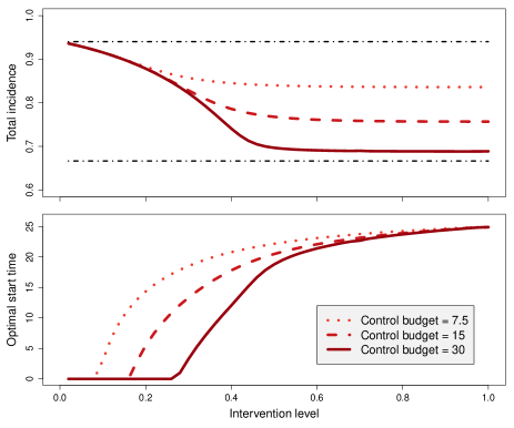
When an epidemic with a basic reproduction number β„›0=3subscriptβ„›03\mathcal{R}_{0}=3 hits an overwhelmingly susceptible population, eventually 94.0% of individuals will become infected if no interventions are imposed. Furthermore, at least 1βˆ’1/(S​(0)​ℛ0)=66.6%11𝑆0subscriptβ„›0percent66.61-1/(S(0)\mathcal{R}_{0})=66.6\% will become infected under an arbitrary intervention with a finite total cost (Theorem 2). The top panel in Fig.Β 1 displays the total incidence that is achievable using optimal strategies with total cost β€–uβ€–1subscriptnorm𝑒1||u||_{1} bounded by c1=7.5,15,30subscript𝑐17.51530c_{1}=7.5,15,30 and maximum intervention level bounded by 0<cβˆžβ‰€10subscript𝑐10<c_{\infty}\leq 1. It is seen that interventions with even a modest budget of c1=7.5subscript𝑐17.5c_{1}=7.5 may significantly reduce total incidence if they can be imposed at a sufficient magnitude. On the other hand, long but mild interventions have little effect on total incidence.

The bottom panel in Fig.Β 1 shows that the higher the maximal intervention level c∞subscript𝑐c_{\infty}, the longer one should wait before imposing the intervention, and that mild interventions should be started immediately. For a complete lockdown (c∞=1subscript𝑐1c_{\infty}=1), the optimal timing is to wait for 24.94 days, corresponding to the time instant at which the uncontrolled epidemic reaches herd immunity.
Refer to caption
Figure 1: Minimum total incidence (top panel) achievable using interventions with total cost β€–uβ€–1≀c1subscriptnorm𝑒1subscript𝑐1||u||_{1}\leq c_{1} and maximum level β€–uβ€–βˆžβ‰€c∞subscriptnorm𝑒subscript𝑐||u||_{\infty}\leq c_{\infty} for c1=7.5,15,30subscript𝑐17.51530c_{1}=7.5,15,30, and a full range of c∞subscript𝑐c_{\infty} (horizontal axis). The horizontal lines at levels 0.666 and 0.940 indicate the lower and upper bounds of TheoremΒ 2. The bottom panel displays the start times of the optimal strategies corresponding to the (c1,c∞)subscript𝑐1subscript𝑐(c_{1},c_{\infty})-pairs.

3.2 Optimal start time

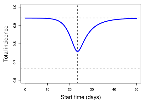
Fig.Β 2 displays the total incidence of a 20-day constant-level lockdown having level 0.75 and total cost 15, for different values of the start time, and underlines the importance of proper timing of such interventions. Mistiming the lockdown even by just one week may have a big effect on number of eventually infected individuals. Somewhat strikingly, starting too early is about equally as bad as starting too late. Similar findings have been reported in [10, 13]. Proper timing is crucial also when minimizing peak prevalence, as noted in [3].
Refer to caption
Figure 2: Total incidence of a constant-level lockdown of duration 20 days and level 0.75, for different values of the start time. The optimal start time t1=23.6subscript𝑑123.6t_{1}=23.6 yields a total incidence of 0.758. The horizontal lines at levels 0.666 and 0.940 indicate the lower and upper bounds of TheoremΒ 2.

3.3 Lack of monotonicity

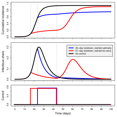
Fig.Β 3 displays a striking phenomenon where adding restrictions before the start of an optimal intervention leads to more individuals eventually becoming infected. The original intervention (blue) with a duration 20 days and a constant level of 0.75, is started optimally at time 23.6. An alternative intervention (red) has the same level and end time but is started seven days earlier. Such a modification, aimed at mitigating disease burden by adding more restrictions, actually has an opposite effect and leads to 19.7% more infections in the long run. This negative outcome is caused by a second wave of infections which starts when the alternative intervention is lifted. This again underlines the important of proper timing: if the longer longer 27-day lockdown were started optimally at time 23.4, the total incidence would have been 0.723 which is not much higher than the best possible outcome of 1βˆ’1/(S​(0)​ℛ0)=0.66611𝑆0subscriptβ„›00.6661-1/(S(0)\mathcal{R}_{0})=0.666 given in TheoremΒ 2. Similar observations manifesting the counterintuitive lack of monotonicity has been reported in [14, 15, 16]. On a positive note, extending interventions from the end will never do harm in this way (see Lemma 8 in the appendix).
Refer to caption
Figure 3: Intervening too early may do more harm than good. An optimally timed 20-day lockdown at 0.75 level is in effect during time interval (23.6,43.6) and leads to a total incidence of 0.758 (blue). A longer but badly timed lockdown at the same level is effective during time interval (16.6, 43.6) and leads to a total incidence of 0.907 (red) which is not far from the total incidence of 0.940 corresponding to an uncontrolled epidemic (black). For the longer 27-day lockdown, the optimal start time is 23.4 and yields total incidence 0.723.

3.4 Comparison with peak-minimizing strategy

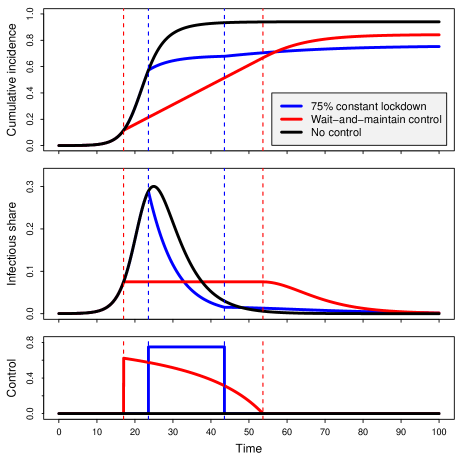
Fig.Β 4 displays time plots of a constant-level lockdown of type (4) designed to minimize total incidence and an intervention of type (3) designed to minimize peak prevalence. Both intervention strategies are constrained by a total budget c1=15subscript𝑐115c_{1}=15 and maximum intervention level c∞=0.75subscript𝑐0.75c_{\infty}=0.75. The latter strategy imposes restrictions earlier, and when these are lifted, the share of infectious individuals in the population is still relatively high, leading to more additional infections and a higher total incidence. As expected, the former strategy yields a lower total incidence than the latter, but at the cost of higher peak prevalence.
Refer to caption
Figure 4: Time plots of cumulative incidence 1βˆ’S​(t)/S​(0)1𝑆𝑑𝑆01-S(t)/S(0) (top), prevalence I​(t)𝐼𝑑I(t) (middle), and intervention level u​(t)𝑒𝑑u(t) (bottom) for three strategies: (a) Total-incidence-minimizing single lockdown of 20 days at 75% level with β€–uβ€–1=15subscriptnorm𝑒115||u||_{1}=15, and optimized start time = 23.6 (blue). (b) Peak-prevalence-minimizing strategy (3) with start time 17.0 and duration 36.6 corresponding to β€–uβ€–1=15subscriptnorm𝑒115||u||_{1}=15 (red). (c) No control (black). The total incidence values for the three strategies are 0.758, 0.843, and 0.940. The corresponding peak prevalence values are 0.289, 0.075, and 0.300.

4 Discussion

It was proven that, among all intervention strategies with cumulative cost not exceeding c1subscript𝑐1c_{1} and magnitude never exceeding c∞subscript𝑐c_{\infty}, a single lockdown at level c∞subscript𝑐c_{\infty}, duration c1/c∞subscript𝑐1subscript𝑐c_{1}/c_{\infty} started at an optimal time instant minimizes the total number of individuals eventually getting infected. As a consequence, assuming that a fixed proportion of infected individuals end up in hospitals and another fixed proportion will die, this strategy also minimizes the cumulative number of hospitalizations and case fatalities. We also saw that the total incidence is at least 1βˆ’1/(S​(0)​ℛ0)11𝑆0subscriptβ„›01-1/(S(0)\mathcal{R}_{0}) for any intervention with a finite total cost. This reflects the fact that in the absence of future vaccinations, the prevalence would start rising again if the susceptible share would be above the herd immunity level 1βˆ’1/β„›011subscriptβ„›01-1/\mathcal{R}_{0} at a time when interventions are relaxed.

Numerically it was seen that milder restrictions for a longer time had very little effect on the total incidence, and also, somewhat surprisingly, that restrictions imposed very early are not as effective as waiting until the prevalence has grown substantially before inserting maximal prevention. Rather counterintuitively, adding restrictions prior to the beginning of an existing intervention strategy may even result in a larger total incidence. On the contrary, as a by-product of our main proof, it was proven that adding restrictions after an intervention strategy has ended can only reduce the total incidence.

The optimization problem is formulated without having any fixed time horizon in mind. If for example a vaccine was known to become available not too far into the future, then this could lead to a rather different optimal prevention. Another assumption was that we were only willing to spend a finite cost c1subscript𝑐1c_{1} for the cumulative preventions. For a severe disease this might not be the case β€” we might be willing to keep some restrictive level for a very long time. In such a case the optimal solution will also be different.

A common feature of epidemic models based on deterministic differential equations is that the fraction of infected individuals never exactly reaches zero. In real epidemics, this might happen due to stochastic finite-population effects. In such cases, a feasible intervention strategy might be to aim for an early elimination of the disease by imposing massive restrictions early on, as has been advocated with SARS-CoV-2 in certain countries. The performance of such strategies cannot be analysed using the type of deterministic models considered here.

The class of interventions considered was assumed to have a bounded linear cost integrated over time. It is not obvious that the societal cost of preventive measures act linearly on the amount of prevention, and therefore nonlinear cost functionals might be relevant to consider. Similarly, changing an existing intervention level might incur additional societal costs, especially if such changes are carried out frequently. The analysis of optimal intervention strategies under such cost functions remains an open problem worthy of attention.

Other extensions worth considering would be to make the underlying epidemic model more realistic by incorporating seasonal effects, adding a latency period between which individuals have been infected but are not yet infectious, including a delay for the time it takes for an intervention decision to take effect, acknowledging different types of individuals and social structures such as households and workplaces, and relaxing the assumption that individuals recover at a constant rate. However, we do not expect major qualitative changes from these extensions, as opposed to considering nonlinear cost functions or unlimited intervention budgets.

5 Proofs

5.1 Proof of TheoremΒ 1

Denote by U​(c1,c∞)π‘ˆsubscript𝑐1subscript𝑐U(c_{1},c_{\infty}) the set of piecewise continuous functions u:[0,∞)β†’[0,1]:𝑒→001u:[0,\infty)\to[0,1] such that β€–uβ€–1≀c1subscriptnorm𝑒1subscript𝑐1||u||_{1}\leq c_{1}Β and β€–uβ€–βˆžβ‰€c∞subscriptnorm𝑒subscript𝑐||u||_{\infty}\leq c_{\infty}. Denote by J​(u)𝐽𝑒J(u)Β the total incidence corresponding to intervention strategy u∈U​(c1,c∞)π‘’π‘ˆsubscript𝑐1subscript𝑐u\in U(c_{1},c_{\infty}). Denote

Jβˆ—=infu∈U​(c1,c∞)J​(u).subscript𝐽subscriptinfimumπ‘’π‘ˆsubscript𝑐1subscript𝑐𝐽𝑒J_{*}\ =\ \inf_{u\in U(c_{1},c_{\infty})}J(u).

Intuition suggests that interventions carried out in a distant future should have a negligible effect on the evolution of the epidemic. PropositionΒ 4 in the appendix confirms this and tells that it is possible to select constants C,Ξ±,Tβˆ—>0𝐢𝛼subscript𝑇0C,\alpha,T_{*}>0Β such that

∫T∞Iu​(t)​𝑑t≀C​eβˆ’Ξ±β€‹Tsuperscriptsubscript𝑇subscript𝐼𝑒𝑑differential-d𝑑𝐢superscript𝑒𝛼𝑇\int_{T}^{\infty}I_{u}(t)\,dt\ \leq\ Ce^{-\alpha T} (5)

for all Tβ‰₯Tβˆ—π‘‡subscript𝑇T\geq T_{*} and all controls bounded by β€–uβ€–1≀c1subscriptnorm𝑒1subscript𝑐1||u||_{1}\leq c_{1}. Let us now fix Ο΅>0italic-Ο΅0\epsilon>0 and choose u1∈U​(c1,c∞)subscript𝑒1π‘ˆsubscript𝑐1subscript𝑐u_{1}\in U(c_{1},c_{\infty}) such that

J​(u1)≀Jβˆ—+Ο΅.𝐽subscript𝑒1subscript𝐽italic-Ο΅J(u_{1})\leq J_{*}+\epsilon. (6)

(i) Truncation. We will approximate u1subscript𝑒1u_{1} by a control u2=1[0,T]​u1subscript𝑒2subscript10𝑇subscript𝑒1u_{2}=1_{[0,T]}u_{1} of finite duration, where we choose a large enough T>Tβˆ—π‘‡subscript𝑇T>T_{*}Β so that C​eβˆ’Ξ±β€‹T≀ϡ𝐢superscript𝑒𝛼𝑇italic-Ο΅Ce^{-\alpha T}\leq\epsilon. Because the trajectories (Su1,Iu1)subscript𝑆subscript𝑒1subscript𝐼subscript𝑒1(S_{u_{1}},I_{u_{1}})Β and (Su2,Iu2)subscript𝑆subscript𝑒2subscript𝐼subscript𝑒2(S_{u_{2}},I_{u_{2}}) coincide up to time T𝑇T, we see that

|J​(u2)βˆ’J​(u1)|=Ξ³S​(0)​|Β β€‹βˆ«T∞Iu2​(t)​𝑑tβˆ’βˆ«T∞Iu1​(t)​𝑑t|𝐽subscript𝑒2𝐽subscript𝑒1𝛾𝑆0Β superscriptsubscript𝑇subscript𝐼subscript𝑒2𝑑differential-d𝑑superscriptsubscript𝑇subscript𝐼subscript𝑒1𝑑differential-d𝑑|J(u_{2})-J(u_{1})|\ =\ \frac{\gamma}{S(0)}\left|Β \int_{T}^{\infty}I_{u_{2}}(t)\,dt-\int_{T}^{\infty}I_{u_{1}}(t)\,dt\right|

BecauseΒ β€–u2β€–1≀‖u1β€–1≀c1subscriptnormsubscript𝑒21subscriptnormsubscript𝑒11subscript𝑐1||u_{2}||_{1}\leq||u_{1}||_{1}\leq c_{1}, inequality (5) tells that both integrals on the right are at most C​eβˆ’Ξ±β€‹T𝐢superscript𝑒𝛼𝑇Ce^{-\alpha T}, and it follows that

|J​(u2)βˆ’J​(u1)|≀ 2​ϡ​γS​(0).𝐽subscript𝑒2𝐽subscript𝑒12italic-ϡ𝛾𝑆0|J(u_{2})-J(u_{1})|\ \leq\ 2\epsilon\frac{\gamma}{S(0)}. (7)

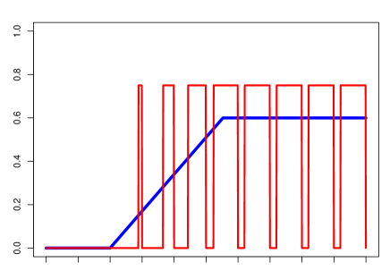
(ii) Quantization. We will next approximate u2subscript𝑒2u_{2} by a bang–bang control u3subscript𝑒3u_{3} defined as follows. We divide time into small intervals Ik=((kβˆ’1)​h,k​h]subscriptπΌπ‘˜π‘˜1β„Žπ‘˜β„ŽI_{k}=((k-1)h,kh] of length 0<h≀ϡ​eβˆ’(Ξ²+Ξ³)​T0β„Žitalic-Ο΅superscript𝑒𝛽𝛾𝑇0<h\leq\epsilon e^{-(\beta+\gamma)T}. We quantize the control function u2subscript𝑒2u_{2} in a frequency modulated fashion so that in each time IksubscriptπΌπ‘˜I_{k}, first u3=0subscript𝑒30u_{3}=0 for hβˆ’Ο„kβ„Žsubscriptπœπ‘˜h-\tau_{k}Β time units, and then u3=c∞subscript𝑒3subscript𝑐u_{3}=c_{\infty} for the remainingΒ Ο„ksubscriptπœπ‘˜\tau_{k} time units, where

Ο„k=bβˆ’1β€‹βˆ«h​kβˆ’hh​ku2​(t)​𝑑tsubscriptπœπ‘˜superscript𝑏1superscriptsubscriptβ„Žπ‘˜β„Žβ„Žπ‘˜subscript𝑒2𝑑differential-d𝑑\tau_{k}\ =\ b^{-1}\int_{hk-h}^{hk}u_{2}(t)\,dt

is selected so that ∫Iku3​(t)​𝑑t=∫Iku2​(t)​𝑑tsubscriptsubscriptπΌπ‘˜subscript𝑒3𝑑differential-d𝑑subscriptsubscriptπΌπ‘˜subscript𝑒2𝑑differential-d𝑑\int_{I_{k}}u_{3}(t)\,dt=\int_{I_{k}}u_{2}(t)\,dt, see FigureΒ 5. As a consequence of h≀ϡ​eβˆ’(Ξ²+Ξ³)​Tβ„Žitalic-Ο΅superscript𝑒𝛽𝛾𝑇h\leq\epsilon e^{-(\beta+\gamma)T}, it follows (details in PropositionΒ 6) that

∫0T|Iu3​(t)βˆ’Iu2​(t)|​𝑑tsuperscriptsubscript0𝑇subscript𝐼subscript𝑒3𝑑subscript𝐼subscript𝑒2𝑑differential-d𝑑\displaystyle\int_{0}^{T}{\lvert I_{u_{3}}(t)-I_{u_{2}}(t)\rvert}\,dt β‰€βˆ«0T3​β​h​e(Ξ²+Ξ³)​t​𝑑tabsentsuperscriptsubscript0𝑇3π›½β„Žsuperscript𝑒𝛽𝛾𝑑differential-d𝑑\displaystyle\ \leq\ \int_{0}^{T}3\beta he^{(\beta+\gamma)t}\,dt
≀ 3​β​h​(Ξ²+Ξ³)βˆ’1​e(Ξ²+Ξ³)​T≀ 3​ϡ.absent3π›½β„Žsuperscript𝛽𝛾1superscript𝑒𝛽𝛾𝑇3italic-Ο΅\displaystyle\ \leq\ 3\beta h(\beta+\gamma)^{-1}e^{(\beta+\gamma)T}\ \leq\ 3\epsilon.

Furthermore,

∫T∞|Iu3​(t)βˆ’Iu2​(t)|​𝑑tβ‰€βˆ«T∞Iu2​(t)​𝑑t+∫T∞Iu3​(t)​𝑑t,superscriptsubscript𝑇subscript𝐼subscript𝑒3𝑑subscript𝐼subscript𝑒2𝑑differential-d𝑑superscriptsubscript𝑇subscript𝐼subscript𝑒2𝑑differential-d𝑑superscriptsubscript𝑇subscript𝐼subscript𝑒3𝑑differential-d𝑑\int_{T}^{\infty}{\lvert I_{u_{3}}(t)-I_{u_{2}}(t)\rvert}\,dt\ \leq\ \int_{T}^{\infty}I_{u_{2}}(t)\,dt+\int_{T}^{\infty}I_{u_{3}}(t)\,dt,

and by noting that β€–u3β€–1=β€–u2β€–1≀c1subscriptnormsubscript𝑒31subscriptnormsubscript𝑒21subscript𝑐1||u_{3}||_{1}=||u_{2}||_{1}\leq c_{1} (LemmaΒ 5), inequality (5) again guarantees that both integrals on the right are at most C​eβˆ’Ξ±β€‹T≀ϡ𝐢superscript𝑒𝛼𝑇italic-Ο΅Ce^{-\alpha T}\leq\epsilon. Hence it follows that

|J​(u3)βˆ’J​(u2)|≀ 5​ϡ​γS​(0).𝐽subscript𝑒3𝐽subscript𝑒25italic-ϡ𝛾𝑆0|J(u_{3})-J(u_{2})|\ \leq\ 5\epsilon\frac{\gamma}{S(0)}. (8)
Refer to caption
Figure 5: Quantization of a function u𝑒u (blue) by frequency modulated function u^^𝑒\hat{u} with amplitude 0.75 (red).

(iii) Prolongation. By construction, u3=cβˆžβ€‹1Asubscript𝑒3subscript𝑐subscript1𝐴u_{3}=c_{\infty}1_{A} where A𝐴A is a finite union of intervals of total length |A|𝐴{\lvert A\rvert}. Because β€–u3β€–1=cβˆžβ€‹|A|subscriptnormsubscript𝑒31subscript𝑐𝐴||u_{3}||_{1}=c_{\infty}{\lvert A\rvert} and β€–u3β€–1=β€–u2β€–1≀c1subscriptnormsubscript𝑒31subscriptnormsubscript𝑒21subscript𝑐1||u_{3}||_{1}=||u_{2}||_{1}\leq c_{1}, we find that |A|≀c1/c∞𝐴subscript𝑐1subscript𝑐{\lvert A\rvert}\leq c_{1}/c_{\infty}. Intuition suggests that a smaller disease burden will be incurred by replacing A𝐴A by a larger subset of the time axis, but such monotonicity properties are known to fail in general (see for example [14, 15]). Nevertheless, prolonging the last interval of A𝐴A from the end does increase the final susceptible share (details in LemmaΒ 8). Let us define u4=cβˆžβ€‹1A~subscript𝑒4subscript𝑐subscript1~𝐴u_{4}=c_{\infty}1_{\tilde{A}}Β where A~~𝐴\tilde{A} is obtained by prolonging the last interval in A𝐴A from the end so that |A~|=c1/c∞~𝐴subscript𝑐1subscript𝑐{\lvert\tilde{A}\rvert}=c_{1}/c_{\infty}. Then it follows that Su4​(∞)β‰₯Su3​(∞)subscript𝑆subscript𝑒4subscript𝑆subscript𝑒3S_{u_{4}}(\infty)\geq S_{u_{3}}(\infty), and therefore, by recalling the equation S​(0)+I​(0)βˆ’Su​(∞)=γ​‖Iuβ€–1𝑆0𝐼0subscript𝑆𝑒𝛾subscriptnormsubscript𝐼𝑒1S(0)+I(0)-S_{u}(\infty)\ =\ \gamma||I_{u}||_{1}, we find that

J​(u4)≀J​(u3).𝐽subscript𝑒4𝐽subscript𝑒3J(u_{4})\ \leq\ J(u_{3}). (9)

(iv) Merging. The control u4subscript𝑒4u_{4} belongs to the set U~~π‘ˆ\tilde{U} of all controls of the form u=cβˆžβ€‹1B𝑒subscript𝑐subscript1𝐡u=c_{\infty}1_{B} where BβŠ‚[0,∞)𝐡0B\subset[0,\infty) is a union of finitely many disjoint intervals of total length c1/c∞subscript𝑐1subscript𝑐c_{1}/c_{\infty}. Among those, the best for minimizing cumulative incidence are those where all disjoint intervals are merged into a single interval of length c1/c∞subscript𝑐1subscript𝑐c_{1}/c_{\infty}. Especially, it is known [7, Theorem 1.1] that there exists Οƒβ‰₯0𝜎0\sigma\geq 0 such that the control u5=cβˆžβ€‹1(Οƒ,Οƒ+c1/c∞)subscript𝑒5subscript𝑐subscript1𝜎𝜎subscript𝑐1subscript𝑐u_{5}=c_{\infty}1_{(\sigma,\sigma+c_{1}/c_{\infty})} satisfies J​(u5)=infu∈U~J​(u)𝐽subscript𝑒5subscriptinfimum𝑒~π‘ˆπ½π‘’J(u_{5})\ =\ \inf_{u\in\tilde{U}}J(u). Especially,

J​(u5)≀J​(u4).𝐽subscript𝑒5𝐽subscript𝑒4J(u_{5})\ \leq\ J(u_{4}). (10)

By collecting the inequalities (6)–(10) together, we conclude that

J​(u5)≀Jβˆ—+8​ϡ​γS​(0).𝐽subscript𝑒5subscript𝐽8italic-ϡ𝛾𝑆0J(u_{5})\ \leq\ J_{*}+8\epsilon\frac{\gamma}{S(0)}.

To summarize, for any Ο΅>0italic-Ο΅0\epsilon>0Β there exists Οƒβ‰₯0𝜎0\sigma\geq 0 such that the single-lockdown control u5=cβˆžβ€‹1(Οƒ,Οƒ+c1/c∞)subscript𝑒5subscript𝑐subscript1𝜎𝜎subscript𝑐1subscript𝑐u_{5}=c_{\infty}1_{(\sigma,\sigma+c_{1}/c_{\infty})} satisfies the above inequality. We conclude that

infu∈U​(c1,c∞)J​(u)=infΟƒβ‰₯0J​(vΟƒ),subscriptinfimumπ‘’π‘ˆsubscript𝑐1subscript𝑐𝐽𝑒subscriptinfimum𝜎0𝐽subscriptπ‘£πœŽ\inf_{u\in U(c_{1},c_{\infty})}J(u)\ =\ \inf_{\sigma\geq 0}J(v_{\sigma}), (11)

where vΟƒ=cβˆžβ€‹1(Οƒ,Οƒ+c1/c∞)subscriptπ‘£πœŽsubscript𝑐subscript1𝜎𝜎subscript𝑐1subscript𝑐v_{\sigma}=c_{\infty}1_{(\sigma,\sigma+c_{1}/c_{\infty})} denotes a single-lockdown control with start time ΟƒπœŽ\sigma, duration c1/c∞subscript𝑐1subscript𝑐c_{1}/c_{\infty}, and constant intervention levelΒ c∞subscript𝑐c_{\infty}.

(v) Timing. Finally, we will verify that the infimum in (11) is attained by an optimally chosen start time Οƒβˆ—β‰₯0subscript𝜎0\sigma_{*}\geq 0. Denote U^=βˆͺΟƒβ‰₯0U^Οƒ^π‘ˆsubscript𝜎0subscript^π‘ˆπœŽ\hat{U}=\cup_{\sigma\geq 0}\hat{U}_{\sigma} where U^Οƒsubscript^π‘ˆπœŽ\hat{U}_{\sigma} is the set of controls such that β€–uβ€–βˆžβ‰€c∞subscriptnorm𝑒subscript𝑐||u||_{\infty}\leq c_{\infty} and u=0𝑒0u=0 outside the time interval [Οƒ,Οƒ+c1/c∞]𝜎𝜎subscript𝑐1subscript𝑐[\sigma,\sigma+c_{1}/c_{\infty}]. Then [10, Theorem 1] implies that there exists a unique Οƒβˆ—β‰₯0subscript𝜎0\sigma_{*}\geq 0 such that

supu∈U^Su​(∞)=supΟƒβ‰₯0supu∈U^ΟƒSu​(∞)=SvΟƒβˆ—β€‹(∞)subscriptsupremum𝑒^π‘ˆsubscript𝑆𝑒subscriptsupremum𝜎0subscriptsupremum𝑒subscript^π‘ˆπœŽsubscript𝑆𝑒subscript𝑆subscript𝑣subscript𝜎\sup_{u\in\hat{U}}S_{u}(\infty)\ =\ \sup_{\sigma\geq 0}\sup_{u\in\hat{U}_{\sigma}}S_{u}(\infty)\ =\ S_{v_{\sigma_{*}}}(\infty)

for vΟƒβˆ—=cβˆžβ€‹1(Οƒ,Οƒ+c1/c∞)subscript𝑣subscript𝜎subscript𝑐subscript1𝜎𝜎subscript𝑐1subscript𝑐v_{\sigma_{*}}=c_{\infty}1_{(\sigma,\sigma+c_{1}/c_{\infty})}. Therefore, by recalling the equation S​(0)+I​(0)βˆ’Su​(∞)=γ​‖Iuβ€–1.𝑆0𝐼0subscript𝑆𝑒𝛾subscriptnormsubscript𝐼𝑒1S(0)+I(0)-S_{u}(\infty)\ =\ \gamma||I_{u}||_{1}., it follows that

infu∈U^J​(u)=J​(vΟƒβˆ—).subscriptinfimum𝑒^π‘ˆπ½π‘’π½subscript𝑣subscript𝜎\inf_{u\in\hat{U}}J(u)\ =\ J(v_{\sigma_{*}}).

Because U^^π‘ˆ\hat{U} contains all controls of the form vΟƒ=cβˆžβ€‹1(Οƒ,Οƒ+c1/c∞)subscriptπ‘£πœŽsubscript𝑐subscript1𝜎𝜎subscript𝑐1subscript𝑐v_{\sigma}=c_{\infty}1_{(\sigma,\sigma+c_{1}/c_{\infty})}, we conclude that

J​(vΟƒβˆ—)=infΟƒβ‰₯0J​(vΟƒ).𝐽subscript𝑣subscript𝜎subscriptinfimum𝜎0𝐽subscriptπ‘£πœŽJ(v_{\sigma_{*}})\ =\ \inf_{\sigma\geq 0}J(v_{\sigma}).

In light of (11), this confirms the statement of the theorem. ∎

5.2 Proof of TheoremΒ 2

For a standard SIR model with no interventions (u=0𝑒0u=0), it is well known that the limiting susceptible share is bounded by S​(∞)≀γβ𝑆𝛾𝛽S(\infty)\leq\frac{\gamma}{\beta}. By a careful reasoning (PropositionΒ 3 in the appendix), the same bound extends to epidemics controlled by an intervention with β€–uβ€–1<∞subscriptnorm𝑒1||u||_{1}<\infty. Therefore, the total incidence is bounded from below by 1βˆ’S​(∞)/S​(0)β‰₯1βˆ’Ξ³/(β​S​(0))1𝑆𝑆01𝛾𝛽𝑆01-S(\infty)/S(0)\geq 1-\gamma/(\beta S(0)).

For the upper bound, it appears intuitively clear that the limiting susceptible share Su​(∞)subscript𝑆𝑒S_{u}(\infty) in an epidemic with an arbitrary control u𝑒u is larger than equal than the corresponding quantity S0​(∞)subscript𝑆0S_{0}(\infty) in an epidemic with no interventions. Indeed, Chikina and Pegden [14] have shown that a pointwise ordering of interventions u1≀u2subscript𝑒1subscript𝑒2u_{1}\leq u_{2} implies Su1​(∞)≀Su2​(∞)subscript𝑆subscript𝑒1subscript𝑆subscript𝑒2S_{u_{1}}(\infty)\leq S_{u_{2}}(\infty) under an extra assumption that u2subscript𝑒2u_{2} is nondecreasing. Straightforward modifications of the analysis in [14] show that the above implication holds also when u1subscript𝑒1u_{1} instead of u2subscript𝑒2u_{2} is required to be nondecreasing. By selecting u1=0subscript𝑒10u_{1}=0 and letting u2=usubscript𝑒2𝑒u_{2}=u be an arbitrary piecewise continuous intervention, we find that S0​(∞)≀Su​(∞)subscript𝑆0subscript𝑆𝑒S_{0}(\infty)\leq S_{u}(\infty), and we conclude that the total incidence is bounded from above by 1βˆ’Su​(∞)/S​(0)≀1βˆ’S0​(∞)/S​(0)1subscript𝑆𝑒𝑆01subscript𝑆0𝑆01-S_{u}(\infty)/S(0)\leq 1-S_{0}(\infty)/S(0). ∎

Acknowledgments

The authors are grateful for financial support from project 105572 NordicMathCovid as part of the Nordic Programme on Health and Welfare funded by NordForsk.

References

  • [1] WilliamΒ Ogilvy Kermack and A.Β G. McKendrick. A contribution to the mathematical theory of epidemics. Proceedings of the Royal Society of London A, 115(772):700–721, 1927.
  • [2] Odo Diekmann, Hans Heesterbeek, and Tom Britton. Mathematical Tools for Understanding Infectious Disease Dynamics. Princeton University Press, 2013.
  • [3] DylanΒ H. Morris, FernandoΒ W. Rossine, JoshuaΒ B. Plotkin, and SimonΒ A. Levin. Optimal, near-optimal, and robust epidemic control. Communications Physics, 4(1):78, 2021.
  • [4] JamesΒ M. Greene and EduardoΒ D. Sontag. Minimizing the infected peak utilizing a single lockdown: a technical result regarding equal peaks. medRxiv, 2021.
  • [5] Laurent Miclo, Daniel Spiro, and JΓΆrgen Weibull. Optimal epidemic suppression under an ICU constraint. arXiv, 2020.
  • [6] Florin Avram, Lorenzo Freddi, and Dan Goreac. Optimal control of a SIR epidemic with ICU constraints and target objectives. Applied Mathematics and Computation, 418:126816, 2022.
  • [7] Yuanyuan Feng, Gautam Iyer, and Lei Li. Scheduling fixed length quarantines to minimize the total number of fatalities during an epidemic. Journal of Mathematical Biology, 82(7):69, 2021.
  • [8] Pierre-Alexandre Bliman, Michel Duprez, Yannick Privat, and Nicolas Vauchelet. Optimal immunity control and final size minimization by social distancing for the SIR epidemic model. Journal of Optimization Theory and Applications, 189(2):408–436, 2021.
  • [9] DavidΒ I. Ketcheson. Optimal control of an sir epidemic through finite-time non-pharmaceutical intervention. Journal of Mathematical Biology, 83(1), Jun 2021.
  • [10] Pierre-Alexandre Bliman and Michel Duprez. How best can finite-time social distancing reduce epidemic final size? Journal of Theoretical Biology, 511:110557, 2021.
  • [11] Leonardo Cianfanelli, Francesca Parise, Daron Acemoglu, Giacomo Como, and Asuman Ozdaglar. Lockdown interventions in SIR model: Is the reproduction number the right control variable?, 2021. arXiv.
  • [12] Seth Flaxman, Swapnil Mishra, Axel Gandy, H.Β JulietteΒ T. Unwin, ThomasΒ A. Mellan, Helen Coupland, Charles Whittaker, Harrison Zhu, Tresnia Berah, JeffreyΒ W. Eaton, MΓ©lodie Monod, PabloΒ N. Perez-Guzman, Nora Schmit, Lucia Cilloni, Kylie E.Β C. Ainslie, Marc Baguelin, Adhiratha Boonyasiri, Olivia Boyd, Lorenzo Cattarino, LauraΒ V. Cooper, Zulma CucunubΓ‘, Gina Cuomo-Dannenburg, Amy Dighe, Bimandra Djaafara, Ilaria Dorigatti, SabineΒ L. van Elsland, RichardΒ G. FitzJohn, Katy A.Β M. Gaythorpe, Lily Geidelberg, NicholasΒ C. Grassly, WilliamΒ D. Green, Timothy Hallett, Arran Hamlet, Wes Hinsley, Ben Jeffrey, Edward Knock, DanielΒ J. Laydon, Gemma Nedjati-Gilani, Pierre Nouvellet, KrisΒ V. Parag, Igor Siveroni, HayleyΒ A. Thompson, Robert Verity, Erik Volz, CarolineΒ E. Walters, Haowei Wang, Yuanrong Wang, OliverΒ J. Watson, Peter Winskill, Xiaoyue Xi, Patrick G.Β T. Walker, AzraΒ C. Ghani, ChristlΒ A. Donnelly, Steven Riley, Michaela A.Β C. Vollmer, NeilΒ M. Ferguson, LucyΒ C. Okell, Samir Bhatt, and Imperial College COVID-19Β Response Team. Estimating the effects of non-pharmaceutical interventions on COVID-19 in Europe. Nature, 584(7820):257–261, 2020.
  • [13] Francesco DiΒ Lauro, IstvΓ‘nΒ Z. Kiss, and JoelΒ C. Miller. Optimal timing of one-shot interventions for epidemic control. PLOS Computational Biology, 17(3):1–25, 03 2021.
  • [14] Maria Chikina and Wesley Pegden. Failure of monotonicity in epidemic models, 2020.
  • [15] Andreas Handel, IraΒ M Longini, and Rustom Antia. What is the best control strategy for multiple infectious disease outbreaks? Proceedings of the Royal Society B: Biological Sciences, 274(1611):833–837, 2007.
  • [16] Thomas Kruse and Philipp Strack. Optimal control of an epidemic through social distancing. SSRN Preprint, 2020.
  • [17] HassanΒ K. Khalil. Nonlinear Systems. Prentice Hall, 1995.

Appendix A Truncation

The appendices present technical details needed for proving TheoremΒ 1. AppendixΒ A contains details related to approximating a control of infinite time horizon by truncation. AppendixΒ B contains an analysis of a frequency-modulated quantization operator. AppendixΒ C contains a monotonicity property related to minimizing the disease burden by prolonged interventions.

A.1 Time to reach herd immunity

For an epidemic trajectory (Su,Iu)subscript𝑆𝑒subscript𝐼𝑒(S_{u},I_{u}) controlled by u𝑒u, we denote the time at which herd immunity is reached by

tH​(u)=inf{tβ‰₯0:Su​(t)≀γβ}.subscript𝑑𝐻𝑒infimumconditional-set𝑑0subscript𝑆𝑒𝑑𝛾𝛽t_{H}(u)\ =\ \inf\left\{t\geq 0:S_{u}(t)\leq\frac{\gamma}{\beta}\right\}.

The following result generalizes [7, Lemma 3.3:(2)] (and corrects a minor mistake in its proof).

Proposition 3.

For any initial state with S​(0)>γβ𝑆0𝛾𝛽S(0)>\frac{\gamma}{\beta} and I​(0)>0𝐼00I(0)>0, and any piecewise continuous control such that β€–uβ€–1<∞subscriptnorm𝑒1||u||_{1}<\infty, the time to reach herd immunity is finite and bounded by

tH​(u)≀‖uβ€–1+log⁑(βγ​S​(0))β​I​(0)​eγ​‖uβ€–1.subscript𝑑𝐻𝑒subscriptnorm𝑒1𝛽𝛾𝑆0𝛽𝐼0superscript𝑒𝛾subscriptnorm𝑒1t_{H}(u)\ \leq\ ||u||_{1}+\frac{\log(\frac{\beta}{\gamma}S(0))}{\beta I(0)}e^{\gamma||u||_{1}}.
Proof.

We will analyse the system on the time interval up to tH=tH​(u)subscript𝑑𝐻subscript𝑑𝐻𝑒t_{H}=t_{H}(u). Observe that the logarithmic state variables evolve according to

(log⁑Su)β€²superscriptsubscript𝑆𝑒′\displaystyle(\log S_{u})^{\prime} =βˆ’Ξ²β€‹(1βˆ’u)​Iu,absent𝛽1𝑒subscript𝐼𝑒\displaystyle\ =\ -\beta(1-u)I_{u}, (12)
(log⁑Iu)β€²superscriptsubscript𝐼𝑒′\displaystyle(\log I_{u})^{\prime} =β​(1βˆ’u)​Suβˆ’Ξ³.absent𝛽1𝑒subscript𝑆𝑒𝛾\displaystyle\ =\ \beta(1-u)S_{u}-\gamma. (13)

By definition, Suβ‰₯Ξ³Ξ²subscript𝑆𝑒𝛾𝛽S_{u}\geq\frac{\gamma}{\beta} on [0,tH]0subscript𝑑𝐻[0,t_{H}]. This lower bound combined with (13) implies that (log⁑Iu)β€²β‰₯βˆ’Ξ³β€‹usuperscriptsubscript𝐼𝑒′𝛾𝑒(\log I_{u})^{\prime}\geq-\gamma u, and therefore

Iu​(t)β‰₯I​(0)​eβˆ’Ξ³β€‹βˆ«0tu​(s)​𝑑sβ‰₯I​(0)​eβˆ’Ξ³β€‹β€–uβ€–1subscript𝐼𝑒𝑑𝐼0superscript𝑒𝛾superscriptsubscript0𝑑𝑒𝑠differential-d𝑠𝐼0superscript𝑒𝛾subscriptnorm𝑒1I_{u}(t)\ \geq\ I(0)e^{-\gamma\int_{0}^{t}u(s)ds}\ \geq\ I(0)e^{-\gamma||u||_{1}} (14)

on [0,tH]0subscript𝑑𝐻[0,t_{H}]. By denoting Imin=I​(0)​eβˆ’Ξ³β€‹β€–uβ€–1subscript𝐼min𝐼0superscript𝑒𝛾subscriptnorm𝑒1I_{\rm min}=I(0)e^{-\gamma||u||_{1}} and combining the above inequality with (12), it follows that (log⁑Su)β€²β‰€βˆ’Ξ²β€‹Imin​(1βˆ’u)superscriptsubscript𝑆𝑒′𝛽subscript𝐼min1𝑒(\log S_{u})^{\prime}\leq-\beta I_{\rm min}(1-u) on [0,tH]0subscript𝑑𝐻[0,t_{H}], so that

log⁑Su​(tH)βˆ’log⁑S​(0)subscript𝑆𝑒subscript𝑑𝐻𝑆0\displaystyle\log S_{u}(t_{H})-\log S(0) β‰€βˆ’Ξ²β€‹Iminβ€‹βˆ«0tH(1βˆ’u​(t))​𝑑tabsent𝛽subscript𝐼minsuperscriptsubscript0subscript𝑑𝐻1𝑒𝑑differential-d𝑑\displaystyle\ \leq\ -\beta I_{\rm min}\int_{0}^{t_{H}}(1-u(t))\,dt
≀β​Imin​(β€–uβ€–1βˆ’tH).absent𝛽subscript𝐼minsubscriptnorm𝑒1subscript𝑑𝐻\displaystyle\ \leq\ \beta I_{\rm min}(||u||_{1}-t_{H}).

By noting that Su​(tH)=Ξ³Ξ²subscript𝑆𝑒subscript𝑑𝐻𝛾𝛽S_{u}(t_{H})=\frac{\gamma}{\beta} by the continuity of Susubscript𝑆𝑒S_{u}, we see that

tH≀‖uβ€–1+log⁑S​(0)βˆ’log⁑γββ​Imin,subscript𝑑𝐻subscriptnorm𝑒1𝑆0𝛾𝛽𝛽subscript𝐼mint_{H}\ \leq\ ||u||_{1}+\frac{\log S(0)-\log\frac{\gamma}{\beta}}{\beta I_{\rm min}},

and the claim follows. ∎

A.2 Uniform integrability

The following result shows that the collection of infectious trajectories induced by controls bounded by β€–uβ€–1≀c1subscriptnorm𝑒1subscript𝑐1||u||_{1}\leq c_{1} is uniformly integrable.

Proposition 4.

For any Ξ²,Ξ³>0𝛽𝛾0\beta,\gamma>0, any initial state with S​(0)>0𝑆00S(0)>0 and I​(0)>0𝐼00I(0)>0, and any c1β‰₯0subscript𝑐10c_{1}\geq 0, there exist constants Ξ±,C,Tβˆ—>0𝛼𝐢subscript𝑇0\alpha,C,T_{*}>0 such that

supβ€–uβ€–1≀c1∫T∞Iu​(t)​𝑑t≀C​eβˆ’Ξ±β€‹Tfor allΒ Tβ‰₯Tβˆ—.subscriptsupremumsubscriptnorm𝑒1subscript𝑐1superscriptsubscript𝑇subscript𝐼𝑒𝑑differential-d𝑑𝐢superscript𝑒𝛼𝑇for allΒ Tβ‰₯Tβˆ—\sup_{||u||_{1}\leq c_{1}}\int_{T}^{\infty}I_{u}(t)\,dt\ \leq\ Ce^{-\alpha T}\qquad\text{for all $T\geq T_{*}$}.
Proof.

(i) PropositionΒ 3 implies that for all controls with β€–uβ€–1≀c1subscriptnorm𝑒1subscript𝑐1||u||_{1}\leq c_{1}, the time to reach herd immunity is bounded by the constant

tHβˆ—=max⁑{c1+Ξ²βˆ’1​I​(0)βˆ’1​log⁑(βγ​S​(0))​eγ​c1, 0}.subscriptsuperscript𝑑𝐻subscript𝑐1superscript𝛽1𝐼superscript01𝛽𝛾𝑆0superscript𝑒𝛾subscript𝑐1 0t^{*}_{H}\ =\ \max\{c_{1}+\beta^{-1}I(0)^{-1}\log(\frac{\beta}{\gamma}S(0))e^{\gamma c_{1}},\,0\}.

Therefore, the susceptible share satisfies Su​(t)≀γβsubscript𝑆𝑒𝑑𝛾𝛽S_{u}(t)\leq\frac{\gamma}{\beta} from time tHβˆ—subscriptsuperscript𝑑𝐻t^{*}_{H} onwards. We will choose a slightly larger time horizon Tβˆ—=tHβˆ—+c1+1subscript𝑇subscriptsuperscript𝑑𝐻subscript𝑐11T_{*}=t^{*}_{H}+c_{1}+1 and show that

Su​(t)≀(1βˆ’Ξ΄)​γβsubscript𝑆𝑒𝑑1𝛿𝛾𝛽S_{u}(t)\ \leq\ (1-\delta)\frac{\gamma}{\beta} (15)

for all tβ‰₯Tβˆ—π‘‘subscript𝑇t\geq T_{*} and all controls u𝑒u such that β€–uβ€–1≀c1subscriptnorm𝑒1subscript𝑐1||u||_{1}\leq c_{1}, where Ξ΄=1βˆ’exp⁑(βˆ’Ξ²β€‹I​(0)​eβˆ’Ξ³β€‹Tβˆ—)𝛿1𝛽𝐼0superscript𝑒𝛾subscript𝑇\delta=1-\exp(-\beta I(0)e^{-\gamma T_{*}}). To verify (15), observe first that

∫tHβˆ—Tβˆ—(1βˆ’u​(t))​𝑑t=c1+1βˆ’βˆ«tHβˆ—Tβˆ—u​(t)​𝑑tβ‰₯c1+1βˆ’β€–uβ€–1β‰₯ 1.superscriptsubscriptsuperscriptsubscript𝑑𝐻subscript𝑇1𝑒𝑑differential-d𝑑subscript𝑐11superscriptsubscriptsuperscriptsubscript𝑑𝐻subscript𝑇𝑒𝑑differential-d𝑑subscript𝑐11subscriptnorm𝑒11\int_{t_{H}^{*}}^{T_{*}}(1-u(t))\,dt\ =\ c_{1}+1-\int_{t_{H}^{*}}^{T_{*}}u(t)\,dt\ \geq\ c_{1}+1-||u||_{1}\ \geq\ 1. (16)

The crude lower bound (log⁑Iu)β€²=β​(1βˆ’u)​Suβˆ’Ξ³β‰₯βˆ’Ξ³superscriptsubscript𝐼𝑒′𝛽1𝑒subscript𝑆𝑒𝛾𝛾(\log I_{u})^{\prime}=\beta(1-u)S_{u}-\gamma\geq-\gamma implies that I​(t)β‰₯I​(0)​eβˆ’Ξ³β€‹Tβˆ—πΌπ‘‘πΌ0superscript𝑒𝛾subscript𝑇I(t)\geq I(0)e^{-\gamma T_{*}} on (0,Tβˆ—)0subscript𝑇(0,T_{*}). By noting that (log⁑S)β€²=βˆ’Ξ²β€‹(1βˆ’u)​Isuperscript𝑆′𝛽1𝑒𝐼(\log S)^{\prime}=-\beta(1-u)I, it follows by (16) that

log⁑Su​(Tβˆ—)βˆ’log⁑Su​(tHβˆ—)=βˆ’Ξ²β€‹βˆ«tHβˆ—Tβˆ—(1βˆ’u​(t))​Iu​(t)​𝑑tsubscript𝑆𝑒subscript𝑇subscript𝑆𝑒superscriptsubscript𝑑𝐻𝛽superscriptsubscriptsuperscriptsubscript𝑑𝐻subscript𝑇1𝑒𝑑subscript𝐼𝑒𝑑differential-d𝑑\displaystyle\log S_{u}(T_{*})-\log S_{u}(t_{H}^{*})\ =\ -\beta\int_{t_{H}^{*}}^{T_{*}}(1-u(t))I_{u}(t)\,dt β‰€βˆ’Ξ²β€‹I​(0)​eβˆ’Ξ³β€‹Tβˆ—.absent𝛽𝐼0superscript𝑒𝛾subscript𝑇\displaystyle\ \leq\ -\beta I(0)e^{-\gamma T_{*}}.

By noting that the right side above equals log⁑(1βˆ’Ξ΄)1𝛿\log(1-\delta), and that Su​(tHβˆ—)≀γβsubscript𝑆𝑒superscriptsubscript𝑑𝐻𝛾𝛽S_{u}(t_{H}^{*})\leq\frac{\gamma}{\beta} due to tH​(u)≀tHβˆ—subscript𝑑𝐻𝑒superscriptsubscript𝑑𝐻t_{H}(u)\leq t_{H}^{*}, we conclude that log⁑Su​(Tβˆ—)≀log⁑γβ+log⁑(1βˆ’Ξ΄),subscript𝑆𝑒subscript𝑇𝛾𝛽1𝛿\log S_{u}(T_{*})\leq\log\frac{\gamma}{\beta}+\log(1-\delta), and that (15) is valid.

(ii) We will next derive an upper bound for the tail integrals of Iusubscript𝐼𝑒I_{u}. By applying (15), we see that for all t>Tβˆ—π‘‘subscript𝑇t>T_{*},

(log⁑Iu)β€²=β​(1βˆ’u)​Suβˆ’Ξ³β‰€Ξ²β€‹(1βˆ’Ξ΄)β€‹Ξ³Ξ²βˆ’Ξ³=βˆ’Ξ³β€‹Ξ΄,superscriptsubscript𝐼𝑒′𝛽1𝑒subscript𝑆𝑒𝛾𝛽1𝛿𝛾𝛽𝛾𝛾𝛿(\log I_{u})^{\prime}\ =\ \beta(1-u)S_{u}-\gamma\ \leq\ \beta(1-\delta)\frac{\gamma}{\beta}-\gamma\ =\ -\gamma\delta,

so that

Iu​(t)≀Iu​(Tβˆ—)​eβˆ’Ξ³β€‹Ξ΄β€‹(tβˆ’Tβˆ—)≀eβˆ’Ξ³β€‹Ξ΄β€‹(tβˆ’Tβˆ—).subscript𝐼𝑒𝑑subscript𝐼𝑒subscript𝑇superscript𝑒𝛾𝛿𝑑subscript𝑇superscript𝑒𝛾𝛿𝑑subscript𝑇I_{u}(t)\ \leq\ I_{u}(T_{*})e^{-\gamma\delta(t-T_{*})}\ \leq\ e^{-\gamma\delta(t-T_{*})}.

By integrating the above inequality, we see that

∫T∞Iu​(t)​𝑑t≀1γ​δ​eβˆ’Ξ³β€‹Ξ΄β€‹(Tβˆ’Tβˆ—)for allΒ Tβ‰₯Tβˆ—.superscriptsubscript𝑇subscript𝐼𝑒𝑑differential-d𝑑1𝛾𝛿superscript𝑒𝛾𝛿𝑇subscript𝑇for allΒ Tβ‰₯Tβˆ—\int_{T}^{\infty}I_{u}(t)\,dt\ \leq\ \frac{1}{\gamma\delta}e^{-\gamma\delta(T-T_{*})}\qquad\text{for all $T\geq T_{*}$}.

Therefore, the claim holds for Ξ±=γ​δ𝛼𝛾𝛿\alpha=\gamma\delta and C=1γ​δ​eγ​δ​Tβˆ—πΆ1𝛾𝛿superscript𝑒𝛾𝛿subscript𝑇C=\frac{1}{\gamma\delta}e^{\gamma\delta T_{*}}. ∎

Appendix B Quantization

We develop a frequency modulation approach to approximate a general piecewise continuous function with a square waveform having a small wavelength. Denote by U​(b)π‘ˆπ‘U(b) the set of piecewise continuous functions u:[0,∞)β†’[0,1]:𝑒→001u:[0,\infty)\to[0,1] such that β€–uβ€–βˆžβ‰€bsubscriptnorm𝑒𝑏||u||_{\infty}\leq b. Given an amplitude b>0𝑏0b>0 and wavelength h>0β„Ž0h>0, we define a quantization operator Qb,h:U​(b)β†’U​(b):subscriptπ‘„π‘β„Žβ†’π‘ˆπ‘π‘ˆπ‘Q_{b,h}:U(b)\to U(b) by setting Qb,h​u=u^subscriptπ‘„π‘β„Žπ‘’^𝑒Q_{b,h}u=\hat{u} with

u^​(t)={bifΒ t∈I,0otherwise,^𝑒𝑑cases𝑏ifΒ t∈I0otherwise\hat{u}(t)\ =\ \begin{cases}b&\quad\text{if $t\in I$},\\ 0&\quad\text{otherwise},\end{cases} (17)

where I=βˆͺkβ‰₯1Ik𝐼subscriptπ‘˜1subscriptπΌπ‘˜I=\cup_{k\geq 1}I_{k} is a union of disjoint intervals Ik=[h​kβˆ’Ο„k,h​k)subscriptπΌπ‘˜β„Žπ‘˜subscriptπœπ‘˜β„Žπ‘˜I_{k}=[hk-\tau_{k},hk) having lengths

Ο„k=bβˆ’1β€‹βˆ«h​kβˆ’hh​ku​(t)​𝑑t.subscriptπœπ‘˜superscript𝑏1superscriptsubscriptβ„Žπ‘˜β„Žβ„Žπ‘˜π‘’π‘‘differential-d𝑑\tau_{k}\ =\ b^{-1}\int_{hk-h}^{hk}u(t)\,dt.

We will show that u^^𝑒\hat{u} approximates u𝑒u well in a weak sense for small wavelengths. We first prove a general approximation property (LemmaΒ 5), and then derive an approximation result of an epidemic trajectory controlled by u^^𝑒\hat{u} (PropositionΒ 6).

A function Ο•:[0,∞)→ℝ:italic-Ο•β†’0ℝ\phi:[0,\infty)\to\mathbb{R} is called locally bounded if β€–Ο•β€–βˆž,t=sup0≀s≀t|ϕ​(s)|subscriptnormitalic-ϕ𝑑subscriptsupremum0𝑠𝑑italic-ϕ𝑠||\phi||_{\infty,t}=\sup_{0\leq s\leq t}{\lvert\phi(s)\rvert} is finite for all t𝑑t, and locally Lipschitz continuous if β€–Ο•β€–Lip,t=sup0≀t1<t2≀t|ϕ​(t2)βˆ’Ο•β€‹(t1)|t2βˆ’t1subscriptnormitalic-Ο•Lip𝑑subscriptsupremum0subscript𝑑1subscript𝑑2𝑑italic-Ο•subscript𝑑2italic-Ο•subscript𝑑1subscript𝑑2subscript𝑑1||\phi||_{{\rm Lip},t}=\sup_{0\leq t_{1}<t_{2}\leq t}\frac{{\lvert\phi(t_{2})-\phi(t_{1})\rvert}}{t_{2}-t_{1}} is finite for all t𝑑t.

Lemma 5.

For anyΒ b,h>0π‘β„Ž0b,h>0 and u∈U​(b)π‘’π‘ˆπ‘u\in U(b), the approximation u^=Qb,h​u^𝑒subscriptπ‘„π‘β„Žπ‘’\hat{u}=Q_{b,h}u defined by (17) satisfies β€–u^β€–1=β€–uβ€–1subscriptnorm^𝑒1subscriptnorm𝑒1||\hat{u}||_{1}=||u||_{1}, and

|∫0t(u^​(s)βˆ’u​(s))​ϕ​(s)​𝑑s|≀b​h​(β€–Ο•β€–βˆž,t+t​‖ϕ‖Lip,t)superscriptsubscript0𝑑^𝑒𝑠𝑒𝑠italic-ϕ𝑠differential-dπ‘ π‘β„Žsubscriptnormitalic-ϕ𝑑𝑑subscriptnormitalic-Ο•Lip𝑑\left|\int_{0}^{t}\big{(}\hat{u}(s)-u(s)\big{)}\phi(s)\,ds\,\right|\ \leq\ bh\left(||\phi||_{\infty,t}+t||\phi||_{{\rm Lip},t}\right)

for all tβ‰₯0𝑑0t\geq 0 and all locally bounded and locally Lipschitz continuous Ο•italic-Ο•\phi.

Proof.

On each interval [h​kβˆ’h,h​k)β„Žπ‘˜β„Žβ„Žπ‘˜[hk-h,hk), the quantized control alternates so that u^=0^𝑒0\hat{u}=0Β for the first hβˆ’Ο„kβ„Žsubscriptπœπ‘˜h-\tau_{k} time units, and then u^=b^𝑒𝑏\hat{u}=b for the remaining Ο„ksubscriptπœπ‘˜\tau_{k} time units. The choice of Ο„ksubscriptπœπ‘˜\tau_{k} then implies that

∫h​kβˆ’hh​ku^​(s)​𝑑s=∫h​kβˆ’hh​ku​(s)​𝑑ssuperscriptsubscriptβ„Žπ‘˜β„Žβ„Žπ‘˜^𝑒𝑠differential-d𝑠superscriptsubscriptβ„Žπ‘˜β„Žβ„Žπ‘˜π‘’π‘ differential-d𝑠\int_{hk-h}^{hk}\hat{u}(s)\,ds\ =\ \int_{hk-h}^{hk}u(s)\,ds (18)

for all kβ‰₯1π‘˜1k\geq 1. By summing both sides of the above equality with respect to kβ‰₯1π‘˜1k\geq 1, we find that β€–u^β€–1=β€–uβ€–1subscriptnorm^𝑒1subscriptnorm𝑒1||\hat{u}||_{1}=||u||_{1}.

Let us now fix tβ‰₯0𝑑0t\geq 0. Denote n=⌊thβŒ‹π‘›π‘‘β„Žn=\left\lfloor\frac{t}{h}\right\rfloor and tk=k​hsubscriptπ‘‘π‘˜π‘˜β„Žt_{k}=kh, and observe that ∫0t(u^​(s)βˆ’u​(s))​ϕ​(s)​𝑑s=βˆ‘k=1nAk+Bnsuperscriptsubscript0𝑑^𝑒𝑠𝑒𝑠italic-ϕ𝑠differential-d𝑠superscriptsubscriptπ‘˜1𝑛subscriptπ΄π‘˜subscript𝐡𝑛\int_{0}^{t}\big{(}\hat{u}(s)-u(s)\big{)}\phi(s)\,ds=\sum_{k=1}^{n}A_{k}+B_{n}, where Ak=∫tkβˆ’1tk(u^​(s)βˆ’u​(s))​ϕ​(s)​𝑑ssubscriptπ΄π‘˜superscriptsubscriptsubscriptπ‘‘π‘˜1subscriptπ‘‘π‘˜^𝑒𝑠𝑒𝑠italic-ϕ𝑠differential-d𝑠A_{k}=\int_{t_{k-1}}^{t_{k}}\big{(}\hat{u}(s)-u(s)\big{)}\phi(s)\,ds and Bn=∫tnt(u^​(s)βˆ’u​(s))​ϕ​(s)​𝑑s.subscript𝐡𝑛superscriptsubscriptsubscript𝑑𝑛𝑑^𝑒𝑠𝑒𝑠italic-ϕ𝑠differential-d𝑠B_{n}=\int_{t_{n}}^{t}\big{(}\hat{u}(s)-u(s)\big{)}\phi(s)\,ds. By applying (18), we find that

Ak=∫tkβˆ’1tk(u^​(s)βˆ’u​(s))​(ϕ​(s)βˆ’Ο•β€‹(tkβˆ’1))​𝑑s.subscriptπ΄π‘˜superscriptsubscriptsubscriptπ‘‘π‘˜1subscriptπ‘‘π‘˜^𝑒𝑠𝑒𝑠italic-ϕ𝑠italic-Ο•subscriptπ‘‘π‘˜1differential-d𝑠\displaystyle A_{k}\ =\ \int_{t_{k-1}}^{t_{k}}\big{(}\hat{u}(s)-u(s)\big{)}\big{(}\phi(s)-\phi(t_{k-1})\big{)}\,ds.

Because |ϕ​(s)βˆ’Ο•β€‹(tkβˆ’1)|≀h​‖ϕ‖Lip,titalic-ϕ𝑠italic-Ο•subscriptπ‘‘π‘˜1β„Žsubscriptnormitalic-Ο•Lip𝑑{\lvert\phi(s)-\phi(t_{k-1})\rvert}\leq h||\phi||_{{\rm Lip},t} for all tkβˆ’1<s<tksubscriptπ‘‘π‘˜1𝑠subscriptπ‘‘π‘˜t_{k-1}<s<t_{k}, and β€–u^βˆ’uβ€–βˆžβ‰€bsubscriptnorm^𝑒𝑒𝑏||\hat{u}-u||_{\infty}\leq b, it follows that

|Ak|≀h​‖ϕ‖Lip,tβ€‹βˆ«tkβˆ’1tk|u^​(s)βˆ’u​(s)|​𝑑s≀b​h2​‖ϕ‖Lip,t.subscriptπ΄π‘˜β„Žsubscriptnormitalic-Ο•Lip𝑑superscriptsubscriptsubscriptπ‘‘π‘˜1subscriptπ‘‘π‘˜^𝑒𝑠𝑒𝑠differential-d𝑠𝑏superscriptβ„Ž2subscriptnormitalic-Ο•Lip𝑑\displaystyle|A_{k}|\ \leq\ h||\phi||_{{\rm Lip},t}\int_{t_{k-1}}^{t_{k}}\big{|}\hat{u}(s)-u(s)\big{|}\,ds\ \leq\ bh^{2}||\phi||_{{\rm Lip},t}.

Furthermore, by noting that tn≀t<tn+hsubscript𝑑𝑛𝑑subscriptπ‘‘π‘›β„Žt_{n}\leq t<t_{n}+h, it follows that

|Bn|β‰€β€–Ο•β€–βˆž,tβ€‹βˆ«tnt|u^​(s)βˆ’u​(s)|​𝑑s≀b​hβ€‹β€–Ο•β€–βˆž,t.subscript𝐡𝑛subscriptnormitalic-ϕ𝑑superscriptsubscriptsubscript𝑑𝑛𝑑^𝑒𝑠𝑒𝑠differential-dπ‘ π‘β„Žsubscriptnormitalic-ϕ𝑑{\lvert B_{n}\rvert}\ \leq\ ||\phi||_{\infty,t}\int_{t_{n}}^{t}\big{|}\hat{u}(s)-u(s)\big{|}\,ds\ \leq\ bh||\phi||_{\infty,t}.

We conclude that

|∫0t(u^​(s)βˆ’u​(s))​ϕ​(s)​𝑑s|superscriptsubscript0𝑑^𝑒𝑠𝑒𝑠italic-ϕ𝑠differential-d𝑠\displaystyle\left|\int_{0}^{t}\big{(}\hat{u}(s)-u(s)\big{)}\phi(s)\,ds\,\right| β‰€βˆ‘k=1n|Ak|+|Bn|absentsuperscriptsubscriptπ‘˜1𝑛subscriptπ΄π‘˜subscript𝐡𝑛\displaystyle\ \leq\ \sum_{k=1}^{n}{\lvert A_{k}\rvert}+{\lvert B_{n}\rvert}
≀b​n​h2​‖ϕ‖Lip,t+b​hβ€‹β€–Ο•β€–βˆž,tabsent𝑏𝑛superscriptβ„Ž2subscriptnormitalic-Ο•Lipπ‘‘π‘β„Žsubscriptnormitalic-ϕ𝑑\displaystyle\ \leq\ bnh^{2}||\phi||_{{\rm Lip},t}+bh||\phi||_{\infty,t}
≀b​h​t​‖ϕ‖Lip,t+b​hβ€‹β€–Ο•β€–βˆž,t.absentπ‘β„Žπ‘‘subscriptnormitalic-Ο•Lipπ‘‘π‘β„Žsubscriptnormitalic-ϕ𝑑\displaystyle\ \leq\ bht||\phi||_{{\rm Lip},t}+bh||\phi||_{\infty,t}.

∎

Proposition 6.

For anyΒ b,h>0π‘β„Ž0b,h>0 and u∈U​(b)π‘’π‘ˆπ‘u\in U(b), any Ξ²,Ξ³>0𝛽𝛾0\beta,\gamma>0 and any initial state with S​(0),I​(0)>0𝑆0𝐼00S(0),I(0)>0, the epidemic trajectories (Su,Iu)subscript𝑆𝑒subscript𝐼𝑒(S_{u},I_{u}) and (Su^,Iu^)subscript𝑆^𝑒subscript𝐼^𝑒(S_{\hat{u}},I_{\hat{u}}) associated with u𝑒u and u^=Qb,h​u^𝑒subscriptπ‘„π‘β„Žπ‘’\hat{u}=Q_{b,h}u satisfy

max⁑{|Su^​(t)βˆ’Su​(t)|,|Iu^​(t)βˆ’Iu​(t)|}≀ 3​β​b​h​e(Ξ²+Ξ³)​tsubscript𝑆^𝑒𝑑subscript𝑆𝑒𝑑subscript𝐼^𝑒𝑑subscript𝐼𝑒𝑑3π›½π‘β„Žsuperscript𝑒𝛽𝛾𝑑\max\Big{\{}{\lvert S_{\hat{u}}(t)-S_{u}(t)\rvert},\,{\lvert I_{\hat{u}}(t)-I_{u}(t)\rvert}\Big{\}}\ \leq\ 3\beta bhe^{(\beta+\gamma)t}

for all tβ‰₯0𝑑0t\geq 0.

Proof.

The epidemic trajectory (Su,Iu)subscript𝑆𝑒subscript𝐼𝑒(S_{u},I_{u}) controlled by u𝑒u is the unique solution to X′​(t)=f​(t,X​(t))superscript𝑋′𝑑𝑓𝑑𝑋𝑑X^{\prime}(t)=f(t,X(t)), X​(0)=(S​(0),I​(0))𝑋0𝑆0𝐼0X(0)=(S(0),I(0)), where f:[0,∞)×ℝ2→ℝ2:𝑓→0superscriptℝ2superscriptℝ2f:[0,\infty)\times\mathbb{R}^{2}\to\mathbb{R}^{2} is defined by

f​(t,X)=[βˆ’Ξ±β€‹(t)​X1​X2,α​(t)​X1​X2βˆ’Ξ³β€‹X2]𝑓𝑑𝑋matrix𝛼𝑑subscript𝑋1subscript𝑋2𝛼𝑑subscript𝑋1subscript𝑋2𝛾subscript𝑋2f(t,X)\ =\ \begin{bmatrix}-\alpha(t)X_{1}X_{2},\\ \alpha(t)X_{1}X_{2}-\gamma X_{2}\end{bmatrix} (19)

and α​(t)=β​(1βˆ’u​(t))𝛼𝑑𝛽1𝑒𝑑\alpha(t)=\beta(1-u(t)). The state space of the system is denoted by 𝒳={X∈[0,1]2:X1+X2≀1}𝒳conditional-set𝑋superscript012subscript𝑋1subscript𝑋21\mathcal{X}=\left\{X\in[0,1]^{2}:X_{1}+X_{2}\leq 1\right\} and we equip it with max norm β€–Xβ€–=max⁑{|X1|,|X2|}norm𝑋subscript𝑋1subscript𝑋2||X||=\max\{{\lvert X_{1}\rvert},{\lvert X_{2}\rvert}\}. The Jacobian matrix of X↦f​(t,X)maps-to𝑋𝑓𝑑𝑋X\mapsto f(t,X) equals

βˆ‚Xf​(t,X)=[βˆ’Ξ±β€‹(t)​X2βˆ’Ξ±β€‹(t)​X1α​(t)​X2α​(t)​X1βˆ’Ξ³].subscript𝑋𝑓𝑑𝑋matrix𝛼𝑑subscript𝑋2𝛼𝑑subscript𝑋1𝛼𝑑subscript𝑋2𝛼𝑑subscript𝑋1𝛾\partial_{X}f(t,X)\ =\ \begin{bmatrix}-\alpha(t)X_{2}&-\alpha(t)X_{1}\\ \alpha(t)X_{2}&\alpha(t)X_{1}-\gamma\end{bmatrix}.

The operator norm of the matrix βˆ‚Xf​(t,X)subscript𝑋𝑓𝑑𝑋\partial_{X}f(t,X)Β induced by the max norm on ℝ2superscriptℝ2\mathbb{R}^{2} is the maximum absolute row sum, which is bounded by

β€–βˆ‚Xf​(t,X)β€–normsubscript𝑋𝑓𝑑𝑋\displaystyle||\partial_{X}f(t,X)|| =max⁑{α​(t)​(|X1|+|X2|),α​(t)​|X2|+|α​(t)​X1βˆ’Ξ³|}absent𝛼𝑑subscript𝑋1subscript𝑋2𝛼𝑑subscript𝑋2𝛼𝑑subscript𝑋1𝛾\displaystyle\ =\ \max\Big{\{}\alpha(t)({\lvert X_{1}\rvert}+{\lvert X_{2}\rvert}),\,\alpha(t){\lvert X_{2}\rvert}+{\lvert\alpha(t)X_{1}-\gamma\rvert}\Big{\}}
≀α​(t)​(|X1|+|X2|)+Ξ³.absent𝛼𝑑subscript𝑋1subscript𝑋2𝛾\displaystyle\ \leq\ \alpha(t)({\lvert X_{1}\rvert}+{\lvert X_{2}\rvert})+\gamma.

Hence β€–βˆ‚Xf​(t,X)‖≀β+Ξ³normsubscript𝑋𝑓𝑑𝑋𝛽𝛾||\partial_{X}f(t,X)||\leq\beta+\gamma for all Xβˆˆπ’³π‘‹π’³X\in\mathcal{X} and tβ‰₯0𝑑0t\geq 0, it follows [17, Lemma 2.2] that f𝑓f is Lipschitz continuous according to

β€–f​(t,X)βˆ’f​(t,Y)‖≀(Ξ²+Ξ³)​‖Xβˆ’Yβ€–for allΒ X,Yβˆˆπ’³Β andΒ tβ‰₯0.normπ‘“π‘‘π‘‹π‘“π‘‘π‘Œπ›½π›Ύnormπ‘‹π‘Œfor allΒ X,Yβˆˆπ’³Β andΒ tβ‰₯0.||f(t,X)-f(t,Y)||\leq(\beta+\gamma)||X-Y||\quad\text{for all $X,Y\in\mathcal{X}$ and $t\geq 0$.} (20)

LetΒ Y:[0,∞)→𝒳:π‘Œβ†’0𝒳Y:[0,\infty)\to\mathcal{X} be the unique solution to Y′​(t)=g​(t,Y​(t))superscriptπ‘Œβ€²π‘‘π‘”π‘‘π‘Œπ‘‘Y^{\prime}(t)=g(t,Y(t)), Y​(0)=(S​(0),I​(0))π‘Œ0𝑆0𝐼0Y(0)=(S(0),I(0)), where g​(t,X)𝑔𝑑𝑋g(t,X) is defined analogously to f​(t,X)𝑓𝑑𝑋f(t,X) but with α​(t)𝛼𝑑\alpha(t)Β in (19) replaced by Ξ±^​(t)=β​(1βˆ’u^​(t))^𝛼𝑑𝛽1^𝑒𝑑\hat{\alpha}(t)=\beta(1-\hat{u}(t)). Then

X​(t)𝑋𝑑\displaystyle X(t) =X​(0)+∫0tf​(s,X​(s))​𝑑s,absent𝑋0superscriptsubscript0𝑑𝑓𝑠𝑋𝑠differential-d𝑠\displaystyle\ =\ X(0)+\int_{0}^{t}f(s,X(s))\,ds,
Y​(t)π‘Œπ‘‘\displaystyle Y(t) =Y​(0)+∫0tg​(s,Y​(s))​𝑑s.absentπ‘Œ0superscriptsubscript0π‘‘π‘”π‘ π‘Œπ‘ differential-d𝑠\displaystyle\ =\ Y(0)+\int_{0}^{t}g(s,Y(s))\,ds.

Because X​(0)=Y​(0)𝑋0π‘Œ0X(0)=Y(0), we find that the difference Z​(t)=Y​(t)βˆ’X​(t)π‘π‘‘π‘Œπ‘‘π‘‹π‘‘Z(t)=Y(t)-X(t)Β satisfies

Z​(t)𝑍𝑑\displaystyle Z(t) =∫0t(f​(s,Y​(s))βˆ’f​(s,X​(s)))​𝑑sabsentsuperscriptsubscript0π‘‘π‘“π‘ π‘Œπ‘ π‘“π‘ π‘‹π‘ differential-d𝑠\displaystyle\ =\ \int_{0}^{t}\Big{(}f(s,Y(s))-f(s,X(s))\Big{)}\,ds
+∫0t(g​(s,Y​(s))βˆ’f​(s,Y​(s)))​𝑑s.superscriptsubscript0π‘‘π‘”π‘ π‘Œπ‘ π‘“π‘ π‘Œπ‘ differential-d𝑠\displaystyle\qquad+\int_{0}^{t}\Big{(}g(s,Y(s))-f(s,Y(s))\Big{)}\,ds.

Inequality (20) shows that β€–f​(s,Y​(s))βˆ’f​(s,X​(s))‖≀(Ξ²+Ξ³)​‖z​(s)β€–normπ‘“π‘ π‘Œπ‘ π‘“π‘ π‘‹π‘ π›½π›Ύnorm𝑧𝑠||f(s,Y(s))-f(s,X(s))||\leq(\beta+\gamma)||z(s)|| for all s𝑠s, and we conclude that the max norm of Z​(t)𝑍𝑑Z(t)Β is bounded by

β€–Z​(t)β€–β‰€βˆ«0t(Ξ²+Ξ³)​‖Z​(s)‖​𝑑s+h​(t),norm𝑍𝑑superscriptsubscript0𝑑𝛽𝛾norm𝑍𝑠differential-dπ‘ β„Žπ‘‘||Z(t)||\ \leq\ \int_{0}^{t}(\beta+\gamma)||Z(s)||\,ds+h(t), (21)

where

h​(t)=β€–βˆ«0t(g​(s,Y​(s))βˆ’f​(s,Y​(s)))​𝑑sβ€–.β„Žπ‘‘normsuperscriptsubscript0π‘‘π‘”π‘ π‘Œπ‘ π‘“π‘ π‘Œπ‘ differential-d𝑠h(t)\ =\ \left|\left|\,\int_{0}^{t}\Big{(}g(s,Y(s))-f(s,Y(s))\Big{)}\,ds\,\right|\right|.

Observe next that

g​(s,Y​(s))βˆ’f​(s,Y​(s))=β​(u​(s)βˆ’u^​(s))​ϕ​(s)​[βˆ’1+1],π‘”π‘ π‘Œπ‘ π‘“π‘ π‘Œπ‘ π›½π‘’π‘ ^𝑒𝑠italic-ϕ𝑠matrix11g(s,Y(s))-f(s,Y(s))\ =\ \beta(u(s)-\hat{u}(s))\phi(s)\begin{bmatrix}-1\\ +1\end{bmatrix},

where ϕ​(s)=Y1​(s)​Y2​(s)italic-ϕ𝑠subscriptπ‘Œ1𝑠subscriptπ‘Œ2𝑠\phi(s)=Y_{1}(s)Y_{2}(s), and hence

h​(t)=β​|∫0t(u​(s)βˆ’u^​(s))​ϕ​(s)​𝑑s|.β„Žπ‘‘π›½superscriptsubscript0𝑑𝑒𝑠^𝑒𝑠italic-ϕ𝑠differential-d𝑠h(t)\ =\ \beta\left|\int_{0}^{t}(u(s)-\hat{u}(s))\phi(s)\,ds\right|.

We also find that |Y1′​(t)|=|Su^​(t)|≀βsuperscriptsubscriptπ‘Œ1′𝑑subscript𝑆^𝑒𝑑𝛽{\lvert Y_{1}^{\prime}(t)\rvert}={\lvert S_{\hat{u}}(t)\rvert}\leq\beta and |Y2′​(t)|=|Iu^​(t)|≀β+Ξ³superscriptsubscriptπ‘Œ2′𝑑subscript𝐼^𝑒𝑑𝛽𝛾{\lvert Y_{2}^{\prime}(t)\rvert}={\lvert I_{\hat{u}}(t)\rvert}\leq\beta+\gamma for all tβ‰₯0𝑑0t\geq 0. Therefore, |ϕ′​(t)|≀2​(Ξ²+Ξ³)​tsuperscriptitalic-ϕ′𝑑2𝛽𝛾𝑑{\lvert\phi^{\prime}(t)\rvert}\leq 2(\beta+\gamma)t, and we conclude that Ο•italic-Ο•\phi is globally Lipschitz continuous according to |ϕ​(t)βˆ’Ο•β€‹(s)|≀2​(Ξ²+Ξ³)​|tβˆ’s|italic-ϕ𝑑italic-ϕ𝑠2𝛽𝛾𝑑𝑠{\lvert\phi(t)-\phi(s)\rvert}\leq 2(\beta+\gamma){\lvert t-s\rvert} for all s,tβ‰₯0𝑠𝑑0s,t\geq 0. LemmaΒ 5 then implies that

h​(t)≀C1+C2​tβ„Žπ‘‘subscript𝐢1subscript𝐢2𝑑h(t)\ \leq\ C_{1}+C_{2}t

for C1=β​b​hsubscript𝐢1π›½π‘β„ŽC_{1}=\beta bh and C2=2​β​b​h​(Ξ²+Ξ³)subscript𝐢22π›½π‘β„Žπ›½π›ΎC_{2}=2\beta bh(\beta+\gamma). By combining this with (21), we conclude that

β€–Z​(t)‖≀C1+C2​t+∫0t(Ξ²+Ξ³)​‖Z​(s)‖​𝑑s,norm𝑍𝑑subscript𝐢1subscript𝐢2𝑑superscriptsubscript0𝑑𝛽𝛾norm𝑍𝑠differential-d𝑠||Z(t)||\ \leq\ C_{1}+C_{2}t+\int_{0}^{t}(\beta+\gamma)||Z(s)||\,ds,

and GrΓΆnwall’s inequality (e.g.Β [17, Lemma 2.1]) then implies that

β€–Z​(t)‖≀C1+C2​t+∫0t(C1+C2​s)​(Ξ²+Ξ³)​e(Ξ²+Ξ³)​(tβˆ’s)​𝑑s.norm𝑍𝑑subscript𝐢1subscript𝐢2𝑑superscriptsubscript0𝑑subscript𝐢1subscript𝐢2𝑠𝛽𝛾superscript𝑒𝛽𝛾𝑑𝑠differential-d𝑠||Z(t)||\ \leq\ C_{1}+C_{2}t+\int_{0}^{t}(C_{1}+C_{2}s)(\beta+\gamma)e^{(\beta+\gamma)(t-s)}ds.

Integration by parts shows that the right side equals C1​e(Ξ²+Ξ³)​t+C2Ξ²+γ​(e(Ξ²+Ξ³)​tβˆ’1)subscript𝐢1superscript𝑒𝛽𝛾𝑑subscript𝐢2𝛽𝛾superscript𝑒𝛽𝛾𝑑1C_{1}e^{(\beta+\gamma)t}+\frac{C_{2}}{\beta+\gamma}\left(e^{(\beta+\gamma)t}-1\right), from which we conclude that

β€–Z​(t)‖≀(C1+C2Ξ²+Ξ³)​e(Ξ²+Ξ³)​t= 3​β​b​h​e(Ξ²+Ξ³)​t,norm𝑍𝑑subscript𝐢1subscript𝐢2𝛽𝛾superscript𝑒𝛽𝛾𝑑3π›½π‘β„Žsuperscript𝑒𝛽𝛾𝑑||Z(t)||\ \leq\ \left(C_{1}+\frac{C_{2}}{\beta+\gamma}\right)e^{(\beta+\gamma)t}\ =\ 3\beta bhe^{(\beta+\gamma)t},

confirming the claim. ∎

Appendix C Prolongation

C.1 A special function

Lemma 7.

For any ρ>0𝜌0\rho>0, the function f​(x)=xβˆ’Οβˆ’1​log⁑x𝑓π‘₯π‘₯superscript𝜌1π‘₯f(x)=x-\rho^{-1}\log x is strictly decreasing on (0,Οβˆ’1]0superscript𝜌1(0,\rho^{-1}], and strictly increasing on [Οβˆ’1,∞)superscript𝜌1[\rho^{-1},\infty), and has a unique minimum value y0=1ρ​(1+log⁑ρ)subscript𝑦01𝜌1𝜌y_{0}=\frac{1}{\rho}(1+\log\rho). The restriction of f𝑓f into (0,Οβˆ’1]0superscript𝜌1(0,\rho^{-1}]Β is invertible, and the corresponding inverse function g:[y0,∞)β†’(0,Οβˆ’1]:𝑔→subscript𝑦00superscript𝜌1g:[y_{0},\infty)\to(0,\rho^{-1}] is strictly decreasing.

Proof.

Because f′​(x)=1βˆ’Οβˆ’1​xβˆ’1superscript𝑓′π‘₯1superscript𝜌1superscriptπ‘₯1f^{\prime}(x)=1-\rho^{-1}x^{-1} we find that f′​(x)<0superscript𝑓′π‘₯0f^{\prime}(x)<0Β for s<Οβˆ’1𝑠superscript𝜌1s<\rho^{-1}, and f′​(x)>0superscript𝑓′π‘₯0f^{\prime}(x)>0Β for x>Οβˆ’1π‘₯superscript𝜌1x>\rho^{-1}. Hence the stated monotonicity properties follow. It also follows that f𝑓f restricted to (0,Οβˆ’1]0superscript𝜌1(0,\rho^{-1}] has a well-defined inverse function g𝑔g. The inverse function rule g′​(y)=1f′​(g​(y))superscript𝑔′𝑦1superscript𝑓′𝑔𝑦g^{\prime}(y)=\frac{1}{f^{\prime}(g(y))} shows that g′​(y)<0superscript𝑔′𝑦0g^{\prime}(y)<0 for all y>y0𝑦subscript𝑦0y>y_{0}, and confirms that g𝑔g is strictly decreasing on [y0,∞)subscript𝑦0[y_{0},\infty). ∎

C.2 Prolonged interventions imply less infections

Lemma 8.

Let (S1,I2)subscript𝑆1subscript𝐼2(S_{1},I_{2}) be an epidemic trajectory controlled by u1subscript𝑒1u_{1} such that u1=0subscript𝑒10u_{1}=0Β outside [0,T]0𝑇[0,T]. Let (S2,I2)subscript𝑆2subscript𝐼2(S_{2},I_{2}) be an epidemic trajectory with the same initial state but a modified control u2=u1+c​1[t1,t2]subscript𝑒2subscript𝑒1𝑐subscript1subscript𝑑1subscript𝑑2u_{2}=u_{1}+c1_{[t_{1},t_{2}]} with T≀t1≀t2𝑇subscript𝑑1subscript𝑑2T\leq t_{1}\leq t_{2}. Then S1​(∞)≀S2​(∞)subscript𝑆1subscript𝑆2S_{1}(\infty)\leq S_{2}(\infty).

Proof.

The epidemic under a control uksubscriptπ‘’π‘˜u_{k} evolves according to Skβ€²=βˆ’Ξ²β€‹(1βˆ’uk)​Sk​Iksuperscriptsubscriptπ‘†π‘˜β€²π›½1subscriptπ‘’π‘˜subscriptπ‘†π‘˜subscriptπΌπ‘˜S_{k}^{\prime}=-\beta(1-u_{k})S_{k}I_{k} and Ikβ€²=β​(1βˆ’uk)​Sk​Ikβˆ’Ξ³β€‹IksuperscriptsubscriptπΌπ‘˜β€²π›½1subscriptπ‘’π‘˜subscriptπ‘†π‘˜subscriptπΌπ‘˜π›ΎsubscriptπΌπ‘˜I_{k}^{\prime}=\beta(1-u_{k})S_{k}I_{k}-\gamma I_{k}. This implies that (Sk+Ik)β€²=βˆ’Ξ³β€‹Iksuperscriptsubscriptπ‘†π‘˜subscriptπΌπ‘˜β€²π›ΎsubscriptπΌπ‘˜(S_{k}+I_{k})^{\prime}=-\gamma I_{k} and (log⁑Sk)β€²=βˆ’Ξ²β€‹(1βˆ’uk)​Iksuperscriptsubscriptπ‘†π‘˜β€²π›½1subscriptπ‘’π‘˜subscriptπΌπ‘˜(\log S_{k})^{\prime}=-\beta(1-u_{k})I_{k}. As a consequence, we find that

(β​(1βˆ’uk)​(Sk+Ik)βˆ’Ξ³β€‹log⁑Sk)β€²= 0superscript𝛽1subscriptπ‘’π‘˜subscriptπ‘†π‘˜subscriptπΌπ‘˜π›Ύsubscriptπ‘†π‘˜β€² 0\Big{(}\beta(1-u_{k})(S_{k}+I_{k})-\gamma\log S_{k}\Big{)}^{\prime}\ =\ 0 (22)

at every time instant in which ukβ€²=0superscriptsubscriptπ‘’π‘˜β€²0u_{k}^{\prime}=0.

Let Vk=Sk+Ikβˆ’Ξ³Ξ²β€‹log⁑Sksubscriptπ‘‰π‘˜subscriptπ‘†π‘˜subscriptπΌπ‘˜π›Ύπ›½subscriptπ‘†π‘˜V_{k}=S_{k}+I_{k}-\frac{\gamma}{\beta}\log S_{k}, the vulnerability of the population under control uksubscriptπ‘’π‘˜u_{k}. Because both controls vanish on (t2,∞)subscript𝑑2(t_{2},\infty) and I1​(∞)=I2​(∞)=0subscript𝐼1subscript𝐼20I_{1}(\infty)=I_{2}(\infty)=0, we find from (22) that

Sk​(∞)βˆ’Ξ³Ξ²β€‹log⁑Sk​(∞)=Vk​(t2),k=1,2.formulae-sequencesubscriptπ‘†π‘˜π›Ύπ›½subscriptπ‘†π‘˜subscriptπ‘‰π‘˜subscript𝑑2π‘˜12S_{k}(\infty)-\frac{\gamma}{\beta}\log S_{k}(\infty)\ =\ V_{k}(t_{2}),\quad k=1,2. (23)

Because both trajectories are equal up to time t1subscript𝑑1t_{1}, we see that V1​(t1)=V2​(t1)subscript𝑉1subscript𝑑1subscript𝑉2subscript𝑑1V_{1}(t_{1})=V_{2}(t_{1}). Because u1=0subscript𝑒10u_{1}=0 on the interval (t1,t2)subscript𝑑1subscript𝑑2(t_{1},t_{2}), (22) shows that V1​(t1)=V1​(t2)subscript𝑉1subscript𝑑1subscript𝑉1subscript𝑑2V_{1}(t_{1})=V_{1}(t_{2}). Analogously, by noting that u2=csubscript𝑒2𝑐u_{2}=c on (t1,t2)subscript𝑑1subscript𝑑2(t_{1},t_{2}), it follows that

(1βˆ’c)​(S2​(t1)+I2​(t1))βˆ’Ξ³Ξ²β€‹log⁑S2​(t1)1𝑐subscript𝑆2subscript𝑑1subscript𝐼2subscript𝑑1𝛾𝛽subscript𝑆2subscript𝑑1\displaystyle(1-c)(S_{2}(t_{1})+I_{2}(t_{1}))-\frac{\gamma}{\beta}\log S_{2}(t_{1})
=(1βˆ’c)​(S2​(t2)+I2​(t2))βˆ’Ξ³Ξ²β€‹log⁑S2​(t2),absent1𝑐subscript𝑆2subscript𝑑2subscript𝐼2subscript𝑑2𝛾𝛽subscript𝑆2subscript𝑑2\displaystyle\ =\ (1-c)(S_{2}(t_{2})+I_{2}(t_{2}))-\frac{\gamma}{\beta}\log S_{2}(t_{2}),

which can be rewritten as

V2​(t2)=V2​(t1)+c​(S2​(t2)+I2​(t2)βˆ’S2​(t1)βˆ’I2​(t1)).subscript𝑉2subscript𝑑2subscript𝑉2subscript𝑑1𝑐subscript𝑆2subscript𝑑2subscript𝐼2subscript𝑑2subscript𝑆2subscript𝑑1subscript𝐼2subscript𝑑1V_{2}(t_{2})\ =\ V_{2}(t_{1})+c(S_{2}(t_{2})+I_{2}(t_{2})-S_{2}(t_{1})-I_{2}(t_{1})).

Because (S2+I2)β€²=βˆ’Ξ³β€‹I2superscriptsubscript𝑆2subscript𝐼2′𝛾subscript𝐼2(S_{2}+I_{2})^{\prime}=-\gamma I_{2}, we see that S2​(t)+I2​(t)subscript𝑆2𝑑subscript𝐼2𝑑S_{2}(t)+I_{2}(t)Β is decreasing, and therefore,

V2​(t2)≀V2​(t1)=V1​(t1)=V2​(t1).subscript𝑉2subscript𝑑2subscript𝑉2subscript𝑑1subscript𝑉1subscript𝑑1subscript𝑉2subscript𝑑1V_{2}(t_{2})\ \leq\ V_{2}(t_{1})\ =\ V_{1}(t_{1})\ =\ V_{2}(t_{1}).

Because of (23), it follows (LemmaΒ 7) that S1​(∞)≀S2​(∞)subscript𝑆1subscript𝑆2S_{1}(\infty)\leq S_{2}(\infty). ∎