Fragmentation Functions for $\Xi^{-}/\bar{\Xi}^{+}$ Using Neural Networks

Abstract

We present a determination of fragmentation functions (FFs) for the octet baryon $\Xi^{-}/\bar{\Xi}^{+}$ from data for single inclusive electron-positron annihilation. Our parametrization in this QCD analysis is provided in terms of a Neural Network (NN). We determine fragmentation functions for $\Xi^{-}/\bar{\Xi}^{+}$ at next-to-leading order and for the first time at next-to-next-to-leading order in perturbative QCD. We discuss the improvement of higher-order QCD corrections, the quality of fit, and the comparison of our theoretical results with the fitted datasets. As an application of our new set of fragmentation functions, named SHKS22, we present predictions for $\Xi^{-}/\bar{\Xi}^{+}$ baryon production in proton-proton collisions at the LHC experiments.

I Introduction

Fragmentation Functions (FFs) are necessary to describe the hadronization process in which partons turn into hadrons in the final state. They are needed to describe hadron production in semi-inclusive processes in electron-positron annihilation (SIA), and, together with parton distribution functions (PDFs) in lepton nucleon scattering and (anti)proton-proton collisions. Parametrizations of FFs for light hadrons, as well as for mesons with charm and bottom quarks, are available since long and the corresponding phenomenology is well established. New improved data are routinely used to improve the existing FF parametrizations, see for example Khalek:2021gxf ; Abdolmaleki:2021yjf and references therein. In recent years, progress has been made also for more specific applications, as for example the determination of transverse momentum dependent FFs Kang:2015msa ; Soleymaninia:2019jqo , FFs for heavier hadrons, like $\Lambda_{c}^{\pm}$ baryons Kniehl:2020szu and medium modified FFs Zurita:2021kli . With more precise data it seems also possible to aim at a combined determination of PDFs and FFs Moffat:2021dji and future experiments, for example at the EIC Aschenauer:2019kzf , will eventually improve our understanding of FFs.

In this work we are interested in a determination of FFs for the production of $\Xi^{-}$ and its anti-particle, i.e. the double-strangeness carrying octet baryon. On the experimental side, most important information about $\Xi^{-}$ production is coming from SIA measurements in $e^{+}e^{-}$ annihilation on the $Z$-boson resonance at the LEP experiments ALPEH ALEPH:1996oqp , DELPHI DELPHI:1995dso and OPAL OPAL:1996gsw . Earlier data are also available from MARKII Klein:1986ws and TASSO TASSO:1983qye ; TASSO:1988qlu at somewhat smaller center-of-mass energies. In recent years, also data for $\Xi^{-}$-production in $pp$ and $\bar{p}p$ collisions have been published, covering center-of-mass energies from $\sqrt{s}=17.3$ GeV at NA61/SHINE NA61SHINE:2020dwg , $\sqrt{s}=200$ GeV at STAR STAR:2006nmo ; Heinz:2007ci , 1.96 TeV at CDF CDF:2011dvx , and up to 7 and 13 TeV at CMS CMS:2011jlm ; CMS:2019isl and ALICE ALICE:2012yqk ; ALICE:2019avo ; ALICE:2020jsh . The relevant energy scale in these collider experiments is the transverse momentum of the produced hadron which is, however, rather low and does not reach values above 10 GeV.

On the theoretical side, the only available analysis of the FF of the $\Xi^{-}$ was made in a statistical approach and used data from $e^{+}e^{-}$ annihilation Bourrely:2003wi . This motivates us to perform a new determination of the $\Xi^{-}$ FF using the by now well established technique of neural networks.

The main motivation of our present study is to determine a new set of $\Xi^{-}/\bar{\Xi}^{+}$ FFs. The universality property of FFs allows us to perform a QCD analysis using all available measurements to determine the FFs for a specific hadron. The FFs extracted in this way can be used to obtain theoretical predictions for other processes, like hadron production in pp collisions. In this paper we present a determination of the FFs of $\Xi^{-}/\bar{\Xi}^{+}$ baryon in which single inclusive electron-positron annihilation (SIA) data are analyzed at next-to-leading order (NLO) and next-to-next-to-leading order (NNLO) accuracy in perturbative QCD.

We hope that our determination of $\Xi^{-}/\bar{\Xi}^{+}$ FFs will provide the necessary ingredient needed to obtain predictions for future measurements in a well-defined reference framework based on independent parton-to-hadron fragmentation in perturbative QCD. Such a reference will be needed to test theoretical ideas about mechanisms for hadron production. With future precise data, a comparison with predictions from perturbative QCD is expected to reveal non-perturbative mechanisms and possible collective phenomena in a high-temperature quark-gluon plasma (QGP). For instance, one of the signatures for creating a QGP is production of strange hadrons in heavy-ion collisions Rafelski:1982pu ; Koch:2017pda . In particular hadrons with low transverse momentum are expected to reflect the properties of the bulk system such as collective expansion, the hadro-chemical composition, and the temperature at freeze-out. Measurements of identified hadrons at low transverse momentum used to extract these properties ALICE:2013mez ; NA44:1996xlh will also profit from theory predictions for higher transverse momenta obtained in a reference framework.

We use the recent publicly available MontBlanc package MontBlanc in our analysis. This package is based on neural networks which are believed to provide a parametrization with minimal bias. This allows us to control the precision of the $\Xi^{-}/\bar{\Xi}^{+}$ FFs, based on an efficient minimization algorithm. The numerical calculations of the hadron production cross-section in $e^{+}e^{-}$ annihilation and the scale evolution of the FFs is also performed in this framework. The fitting methodology in the framework of this package has been developed by the NNPDF Collaboration NNPDF:2017mvq ; Khalek:2021gxf ; Bertone:2017tyb .

We will discuss in detail the novel aspects of the methodology used in SHKS22 analysis, the fit quality, the perturbative convergence upon inclusion of higher-order QCD correction, and the stability upon variations of the kinematic cuts applied to the SIA dataset. We will also show that the inclusion of higher-order QCD corrections in our analysis improves the description of the analyzed SIA data.

The structure of the paper is as follows: In Sec. II we review the theoretical formalism for inclusive hadron production in electron-positron annihilation. In Sec. III our methodology based on a neural network (NN) framework is presented. We illustrate the Monte Carlo methodology adopted in our analysis to calculate the uncertainties of FFs and the optimal fit in Sec. IV. In Section V we describe our selection of SIA experimental data included in this study. Details of our new SHKS22 FFs are presented in Sec. VI. We also discuss in this section the impact of higher-order perturbative QCD (pQCD) corrections and compare numerical results for the differential cross sections with the analyzed experimental datasets. In Sec. VII, we present and discuss some predictions for possible future measurements at hadron colliders. Finally, we summarize our conclusions in Sec. VIII.

II QCD Framework

For single inclusive hadron production in electron-positron annihilation, the differential cross-section is given by the formula

$$\frac{d\sigma^{\it h}}{dz}(z,Q^{2})=\frac{4\pi\alpha^{2}(Q)}{Q^{2}}F^{\it h}(z,Q^{2})\,,$$ (1)

where $F^{h}$ is the fragmentation structure function, and $\alpha$ is the QED running coupling. We follow the standard collinear factorization framework esw-book where the QCD cross-sections can be factorized into perturbatively calculable partonic hard cross sections and non-perturbative distribution functions. Thus the structure function is given as a convolution of FFs and hard-scattering coefficient functions:

$$F^{\it h}(z,Q^{2}) = \frac{1}{n_{f}}\sum_{q}^{n_{f}}\hat{e}^{2}_{q}(Q)\times$$

$$\left[D^{\it h}_{S}(z,Q^{2})\otimes C^{S}_{2,q}(z,\alpha_{s}(Q))\right.$$

$$+D^{h}_{g}(z,Q^{2})\otimes C^{S}_{2,g}(z,\alpha_{s}(Q))$$

$$\left.+D^{\it h}_{\rm NS}(z,Q^{2})\otimes C^{\rm NS}_{2,q}(z,\alpha_{s}(Q))\right]\,,$$

where $\hat{e}_{q}(Q)$ are scale-dependent quark electroweak charge factors. Their definition can be found in Ref. Rijken:1996ns . In Eq. (II), the function $D^{h}_{g}(z,Q^{2})$ represents the gluon FF, and $D^{\it h}_{S}(z,Q^{2})$ and $D^{\it h}_{\rm NS}(z,Q^{2})$ are the singlet and non-singlet combinations of FFs which can be written as

$$D_{S}^{\it h}(z,Q^{2}) = \sum_{q}^{n_{f}}D^{\it h}_{q^{+}}(z,Q^{2})\,,$$ (3)

$$D_{\rm NS}^{\it h}(z,Q^{2}) = \sum_{q}^{n_{f}}\frac{\hat{e}^{2}_{q}}{\left<\hat{e}^{2}\right>}\left[D^{\it h}_{q^{+}}(z,Q^{2})-D_{S}^{\it h}(z,Q^{2})\right],$$ (4)

with $D^{h}_{q^{+}}=D^{h}_{q}+D^{h}_{\bar{q}}$. The coefficient functions $C^{S,NS}_{q,g}(z,\alpha_{s}(Q))$ for the singlet and non-singlet combinations have been computed up to $\cal{O}$ $(\alpha_{s}^{2})$ Blumlein:2006rr ; Rijken:1996npa . The average of the effective quark electroweak charges over the number of active flavors reads

$$\left<\hat{e}^{2}\right>=\frac{1}{n_{f}}\sum_{q}^{n_{f}}\hat{e}^{2}_{q}(Q).$$ (5)

The evolution of FFs with the energy scale $Q$ is performed by the standard DGLAP evolution equation Gribov:1972ri ; Altarelli:1977zs ; Dokshitzer:1977sg . The evolution of the singlet combination of FFs mixes with the gluon FF and is given by

$$\frac{\partial}{\partial\ln Q^{2}}\left(\begin{array}[]{c}D_{S}^{h}\\ D_{g}^{h}\end{array}\right)(z,Q^{2}) = \left(\begin{array}[]{cc}P^{qq}&2n_{f}P^{gq}\\ \frac{1}{2n_{f}}P^{qg}&P^{gg}\end{array}\right)\left(z,\alpha_{s}\right)$$ (10)

$$\otimes \left(\begin{array}[]{c}D_{S}^{h}\\ D_{g}^{h}\end{array}\right)(z,Q^{2})\,\mbox{,}$$ (13)

while for the nonsinglet combination of FFs, the DGLAP equation can be written as

$$\frac{\partial}{\partial\ln Q^{2}}D_{\rm NS}^{h}(z,Q^{2})=P^{+}\left(z,\alpha_{s}\right)\otimes D_{\rm NS}^{h}(z,Q^{2})\,\mbox{,}$$ (14)

where $P^{ji}$ and $P^{+}$ are the time-like splitting functions which have a perturbative expansion in terms of the strong coupling constant $\alpha_{s}$,

$$P^{ji,+}\left(z,\alpha_{s}\right)=\sum_{l=0}a_{s}^{l+1}\,P^{ji,+\,(l)}(z)\,\mbox{,}$$ (15)

where $i,j=g,q$ and $a_{s}\equiv\alpha_{s}/(4\pi)$. The time-like splitting functions have been calculated up to $\mathcal{O}(a_{s}^{3})$ in the $\overline{\rm MS}$ scheme and can be found in Refs. Mitov:2006ic ; Moch:2007tx ; Almasy:2011eq .

The calculation of FFs in our analysis is defined in the zero-mass variable-flavor-number scheme (ZM-VFNS) where all active flavors are treated as massless quarks. Nevertheless, a dependence on the heavy-quark masses enters through the fact that the FFs for heavy-quark contributions exhibit a threshold: at scales below the heavy-quark mass the scale evolution is stopped and the FFs are kept constant. We use $m_{c}=1.51$ GeV and $m_{b}=4.92$ GeV for the charm and bottom thresholds, respectively. We choose $\alpha_{s}(M_{Z})=0.118$ as a reference value which is close to the world-average of the Particle Data Group ParticleDataGroup:2018ovx .

III Methodology and Input Parameterization

In this section we present the methodology applied in the SHKS22 analysis, namely the neural network (NN) technique, and describe the basic assumption for the input FFs parameterization. A neural network can be viewed as a complicated prescription to parametrize a function. The architecture of the network, i.e. in particular the number of layers and nodes and the way how nodes are connected, determines the complexity of this parametrization. The typical number of parameters needed to fix a NN is around 100, or more. This is much larger than the number of parameters used in conventional approaches, where simple functional forms for FFs requires to specify in the order of 15 to 30 parameters. Therefore, NNs are expected to be much more flexible and the bias due to the choice of a specific functional form is greatly reduced. For more detailed information about the neural network approach we refer to Refs. Bertone:2017tyb ; Khalek:2021gxf .

The $\Xi^{-}+\bar{\Xi}^{+}$ fragmentation functions for a parton flavor of flavor combination $i$ in terms of a neural network is defined at the initial scale $Q_{0}=5$ GeV by

$$zD^{\Xi^{-}+\bar{\Xi}^{+}}_{i}(z,Q_{0})=(N_{i}(z,\theta)-N_{i}(1,\theta))^{2}\,,$$ (16)

where $N_{i}(z,\theta)$ is a one-layered feed-forward neural network, and $\theta$ denotes the parameter set. The neural network architecture is $[I,N,O]$ where $I$ is the number of input nodes, $N$ denotes the number of intermediate nodes and $O$ is the number of output nodes. We choose a neural network with a single input node describing the scaling variable $z$, a sigmoid activation function for $20$ intermediate nodes and a linear activation function for $3$, $5$ or $6$ output nodes corresponding to the flavor combinations in three different FF sets, I, II or III, respectively, which we will introduce in the following.

SIA experimental measurements are available only for the production of the sum of $\Xi^{-}$ and its antiparticle $\bar{\Xi}^{+}$. The fragmentation structure functions in Eq. (II) do not distinguish between quark and antiquark FFs, i.e. we can only determine the combinations $D^{h}_{q^{+}}=D^{h}_{q}+D^{h}_{\bar{q}}$ with $h=\Xi^{-}+\bar{\Xi}^{+}$. The singlet and non-singlet combinations and the gluon FF enter with different coefficients in the SIA cross section and a separation of these three components can be expected provided data for the $z$ and $Q$ dependence are precise enough.

Our baseline FF parametrization, set I, is chosen assuming the following flavor combinations:

$$zD^{\Xi^{-}+\bar{\Xi}^{+}}_{d^{+}+s^{+}},~{}zD^{\Xi^{-}+\bar{\Xi}^{+}}_{u^{+},c^{+},b^{+}},~{}zD^{\Xi^{-}+\bar{\Xi}^{+}}_{g}\,.$$ (17)

Since the favored quark flavors in the hadron state $\Xi^{-}$ are $(dss)$ and the value of the corresponding electroweak charges $\hat{e}_{q}$ for $d$ and $s$ quarks are the same, we adopt the specific combination $d^{+}+s^{+}$, as was done also in Ref. Binnewies:1994ju . In addition we assume complete symmetry between the disfavored quarks $u^{+}$, $c^{+}$ and $b^{+}$. Therefore, in total we choose $3$ independent flavor combinations corresponding to the neural network architecture $[1,20,3]$.

The FFs for up- and down-type quarks can be separated because they contribute with different charge factors to the cross section. A separation of the heavy-quark components will be possible if charm- or bottom-tagged data become available. At present, there are no heavy-flavor tagged data and it is unlikely that the precision is high enough to be useful for a further separation of flavors, beyond our ansatz described above. Nevertheless, as a test of our approach, we will also study two extended sets, namely set II, assuming the following combinations of FFs:

$$zD^{\Xi^{-}+\bar{\Xi}^{+}}_{d^{+}+s^{+}},~{}zD^{\Xi^{-}+\bar{\Xi}^{+}}_{u^{+}},~{}zD^{\Xi^{-}+\bar{\Xi}^{+}}_{c^{+}},~{}zD^{\Xi^{-}+\bar{\Xi}^{+}}_{b^{+}},~{}zD^{\Xi^{-}+\bar{\Xi}^{+}}_{g},$$

where, in addition to the light quarks and the gluon, we assume separate parametrizations for the heavy quarks $c^{+}$ and $b^{+}$, and set III where all flavors are described by different FFs:

$$zD^{\Xi^{-}/\bar{\Xi}^{+}}_{d^{+}},zD^{\Xi^{-}/\bar{\Xi}^{+}}_{u^{+}},zD^{\Xi^{-}/\bar{\Xi}^{+}}_{s^{+}},zD^{\Xi^{-}/\bar{\Xi}^{+}}_{c^{+}},zD^{\Xi^{-}/\bar{\Xi}^{+}}_{b^{+}},$$

$$zD^{\Xi^{-}/\bar{\Xi}^{+}}_{g}$$ (19)

Thus, for set II (III) we increase the number of independent distribution functions to $5$ ($6$) and the NN architecture is $[1,20,5]$ ($[1,20,6]$). We study sets II and III in order to investigate how well FFs are restricted by data and which uncertainty could be generated by choosing a specific, possibly too general, parametrization. One can find similar approaches in the previous literature.

The number of parameters needed to specify the chosen NN architectures are $103$, $145$ and $166$ for sets I, II and III, respectively. Due to the redundancy of these parameters inherent to the NN architecture by construction, the number of independent parameters is, however, much smaller and usually difficult to determine. Therefore we will not quote $\chi^{2}$ values per degree of freedom, but rather follow the general convention and show $\chi^{2}$ normalized to the number of data points when we compare the fit quality in the following.

IV Monte Carlo Procedure and Determination of the Optimal Fit

There are mainly two methods used in the literature to obtain a reliable determination of the uncertainties of FFs. One of them is the iterative Hessian approach which has been used for example in the DEHSS analysis deFlorian:2014xna ; deFlorian:2017lwf and has been developed in Refs. Pumplin:2000vx ; Pumplin:2001ct . The other important one, developed in Ref. Sato:2016tuz , is the Monte Carlo procedure used in the recent JAM Moffat:2021dji ; Sato:2016wqj and NNFF Bertone:2017tyb fits. We adopt the statistical framework in our SHKS22 analysis.

The MontBlanc framework Khalek:2021gxf utilizes Monte Carlo together with NNs to extract information about the FFs and their uncertainty from the experimental data. The available data are used to generate a discrete sample of FF values, and NNs are employed to interpolate between data points which is needed in order to approximate the required integrations. The first step is training of the NN and creating $N_{\mathrm{rep}}$ replicas of NNs corresponding to pseudo-datasets. Minimization of an appropriately chosen $\chi^{2}$ allows one to choose NNs such that they reproduce a probability distribution of measured points and theoretical predictions with the same mean, variance and correlation as the experimental data. We refer the reader to Refs. Forte:2002fg ; Sato:2016wqj ; Khalek:2021gxf ; Bertone:2017tyb and references therein for a detailed discussion of the approach.

The Monte Carlo approach assumes that the experimental data follow a multivariate Gaussian distribution,

$$\mathcal{G}(\boldsymbol{x}^{k})\propto\exp\left(\left(\boldsymbol{x}^{k}-\boldsymbol{\mu}\right)^{T}\cdot\boldsymbol{C}^{-1}\left(\boldsymbol{x}^{k}-\boldsymbol{\mu}\right)\right),$$ (20)

where $\boldsymbol{x}^{k}=\left\{x_{1}^{k},x_{2}^{k},\cdots,x_{N_{\mathrm{dat}}}^{k}\right\}$ are so called “replicas”, i.e. pseudo-datasets for a set of $N_{\mathrm{dat}}$ measured data points. The vector of expectation values of this distribution is $\boldsymbol{\mu}$ which corresponds to experimental data, and $\boldsymbol{C}$ is the covariance matrix of the data which contains all information on the uncertainties and correlations. The elements of the covariance matrix are defined as in Ref. Khalek:2021gxf ,

$$C_{ij}=\delta_{ij}\sigma_{i,\mathrm{unc}}^{2}+\sum_{\beta}\sigma_{i,\mathrm{corr}}^{(\beta)}\sigma_{j,\mathrm{corr}}^{(\beta)},$$ (21)

where $\sigma_{i,\mathrm{unc}}^{2}$ denotes the sum of squares of all uncorrelated uncertainties, such as the statistical and systematic uncertainties for the $i$th data point and $\sigma_{i,\mathrm{corr}}^{(\beta)}$ is the correlated uncertainty due to $\beta$ source for the same point.

The Monte Carlo approach for the uncertainty propagation uses $N_{\mathrm{rep}}$ replicas of the measured data, $\boldsymbol{x}^{k}$, to turn the experimental uncertainty into that of the NNs that parametrize the FFs. For this purpose, the covariance matrix $\boldsymbol{C}$ is decomposed to a lower triangular $\boldsymbol{L}$ using Cholesky method ($\boldsymbol{C}=\boldsymbol{L}\cdot\boldsymbol{L}^{T}$). If one applies this matrix to an $N_{\mathrm{dat}}$-dimensional Gaussian random vector, $\boldsymbol{r}^{k}$, a vector with the covariance properties of the experimental data is obtained. Accordingly the pseudo dataset is constructed as follows (by Ceres Solver ceres-solver ),

$$\boldsymbol{x}^{k}=\boldsymbol{\mu}+\boldsymbol{L}\cdot\boldsymbol{r}^{k}$$ (22)

This procedure ensures that for sufficiently large $N_{\mathrm{rep}}$, the set of replicas satisfies the following conditions Khalek:2021gxf ,

$$\frac{1}{N_{\mathrm{rep}}}\sum_{k}^{N_{\mathrm{rep}}}{x}^{k}_{i}\simeq\mu_{i}\,,\quad\frac{1}{N_{\mathrm{rep}}}\sum_{k}^{N_{\mathrm{rep}}}{x}^{k}_{i}{x}^{k}_{j}\simeq\mu_{i}\mu_{j}+C_{ij}\,.$$ (23)

At the end of the QCD analysis, a set of $N_{\mathrm{rep}}$ trained NNs are gained and this allows us to estimate the functional integral by averaging over the set of replicas. Notably, estimates for expectation value, uncertainty and correlation of the distribution of an observable $\mathcal{D}$, e.g. a cross section, is given by Forte:2002fg ,

$$\left<\mathcal{D}(x)\right>=\frac{1}{N_{\mathrm{rep}}}\sum_{k=1}^{N_{\mathrm{rep}}}\mathcal{D}^{k}(x)\,,$$

$$\sigma_{\mathcal{D}}=\sqrt{\left<\mathcal{D}^{2}\right>-\left<\mathcal{D}\right>^{2}}\,,$$

$$c_{\mathcal{D}}^{ij}=\frac{\left<\mathcal{D}_{i}\mathcal{D}_{j}\right>-\left<\mathcal{D}_{i}\right>\left<\mathcal{D}_{j}\right>}{\sigma_{i}\sigma_{j}}\,.$$ (24)

In the SHKS22 FFs analysis, we have chosen to include $N_{\mathrm{rep}}=300$, although already a smaller number of replicas, say 200, could be enough to obtain a sub $1\%$ accuracy, see Ref. Khalek:2021gxf .

V Experimental Data

Experiment	$\sqrt{s}$	$N_{\mathrm{dat}}(z>z_{min})$	$\chi^{2}/N_{\mathrm{dat}}$ Set I(NLO)	$\chi^{2}/N_{\mathrm{dat}}$ Set II(NLO)	$\chi^{2}/N_{\mathrm{dat}}$ Set III(NLO)	$\chi^{2}/N_{\mathrm{dat}}$ Set I(NNLO)
ALEPH ALEPH:1996oqp	91.2	8	1.860	2.039	2.035	1.714
DELPHI DELPHI:1995dso	91.2	4	0.659	0.660	0.668	0.673
OPAL OPAL:1996gsw	91.2	5	1.552	1.682	1.726	1.434
MARKII Klein:1986ws	29	4	2.348	2.399	2.428	2.171
TASSO-34 TASSO:1983qye	34	3	1.747	1.805	1.807	1.700
TASSO-34.8 TASSO:1988qlu	34.8	3	0.810	0.731	0.777	0.891
Total $\chi^{2}/N_{\mathrm{dat}}$		27	1.540	1.631	1.643	1.451

Table 1: The list of input datasets for $\Xi^{-}+\bar{\Xi}^{+}$ production included in the SHKS22 analysis. For each dataset we indicate the corresponding reference and the center-of-mass energy $\sqrt{s}$. The number of data points $N_{\mathrm{dat}}$ that satisfy the kinematic cut ($z>0.1$) is displayed in the third column. In columns 4, 5, and 6 we show the value of $\chi^{2}$ per point resulting from the FF fit at NLO for set I, set II and set III, respectively. The last column shows, correspondingly, the $\chi^{2}$ values for the NNLO fit. The last row contains the total values of $\chi^{2}$ divided by the number of data points.

The data included in our analysis is obtained from SIA measurements of the sum of cross sections for $\Xi^{-}$ and $\bar{\Xi}^{+}$ production. We make use of all available experimental data reported by the ALEPH ALEPH:1996oqp , DELPHI DELPHI:1995dso and OPAL OPAL:1996gsw Collaborations at CERN, the MARKII Collaboration Klein:1986ws at SLAC, and the TASSO Collaboration TASSO:1983qye ; TASSO:1988qlu at DESY. The datasets are summarized in Table 1. All the data are for inclusive untagged cross-section measurements. The ALEPH, DELPHI and OPAL data are presented as multiplicities $1/{\sigma_{tot}}d\sigma/dx_{p}$ normalized to the total cross-section at the center-of-mass energy of $\sqrt{s}=M_{Z}$. Here, $x_{p}=2|\mathbb{P_{h}}|/\sqrt{s}$ is the scaled hadron three-momentum. Alternatively, one can also use $z=2E_{h}/\sqrt{s}$, i.e. the energy of the hadron $h$ scaled to the beam energy $\sqrt{s}/2$. The relation between these two scaling variables is given by

$$z=x_{p}\sqrt{1+\frac{4}{x_{p}^{2}}\frac{m_{h}^{2}}{s}}=2\sqrt{\frac{m_{h}^{2}+|\mathbb{P_{h}}|^{2}}{s}}.$$ (25)

The data from the MARKII and TASSO Collaborations are given in different formats. While the TASSO-34.8 data are differential cross-sections $d\sigma/dp_{h}$ measured at the center-of-mass energy $\sqrt{s}=34.8$ GeV, the observables for the MARKII and TASSO-34 data are rescaled cross sections and reported for $(s/\beta)d\sigma/dz$ at the center-of-mass energies $\sqrt{s}=29$ GeV and $\sqrt{s}=34$ GeV, respectively. The parameter $\beta=|\mathbb{P_{h}}|/E_{h}$ is the velocity of the final state hadron $h$.

$z_{min}$ cut	number of data points	$\chi^{2}/N_{\mathrm{dat}}$
0.02	36	4.412
0.05	34	1.967
0.075	31	2.010
0.1	27	1.540

Table 2: The dependence on the kinematical cut, $z_{min}$, (first column) of the number of data points with $z>z_{min}$ analyzed in the fits (second column) and the resulting $\chi^{2}/N_{\mathrm{dat}}$ in the SHKS22 fit set I at NLO.

Figure 1: Dependence of the fit quality, $\chi^{2}/N_{\mathrm{dat}}$, at NLO on the minimum cut values of $z$ for the SIA datasets used in the SHKS22 analysis for set I.

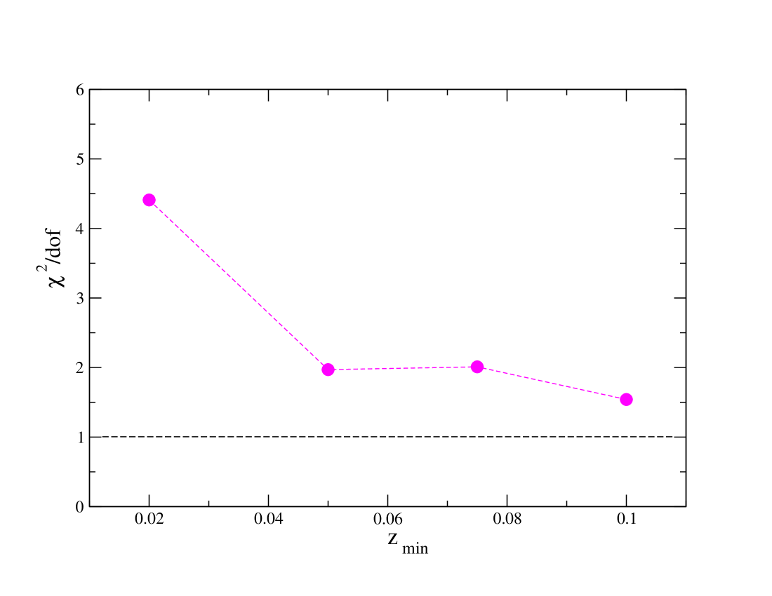
We select data for which a description in the framework of perturbative QCD can be expected to work well and exclude the range of very small values of $z$. Higher-order corrections are known to contain potentially large logarithms proportional to $\ln z$ and $\ln(1-z)$. Since the available data are limited to the range $z<0.5$ we do not have to consider a cut for the large $z$ region. However, we have to carefully choose a lower kinematical cut for $z$. In order to do so, we study the sensitivity of $\chi^{2}/N_{\mathrm{dat}}$ to the variations of $z_{min}$ at NLO accuracy. We scan $z_{min}$ over the region $0.02\leq z\leq 0.1$. The summary of our selection of $z_{min}$ is presented in Table. 2. The first and second columns of this table show our choice of $z$ and the remaining number of data points, respectively. The total number of data without imposing the cut is $36$ points and all of these data points are used in the analysis with $z_{min}=0.02$ cut. In the third column, we report $\chi^{2}/N_{\mathrm{dat}}$ determined from the analyses with different numbers of data and minimum $z$ cuts.

In Fig. 1, the dependence of $\chi^{2}/N_{\mathrm{dat}}$ on the minimum cut value of $z$ is presented. One can conclude from this figure that the optimal $\chi^{2}/N_{\mathrm{dat}}$ value at NLO is obtained by a fit to data with $z_{min}=0.1$. We find that there is no further improvement on $\chi^{2}/N_{\mathrm{dat}}$ by increasing the number of data points and reducing $z_{min}$ to values below $0.1$. We choose the cut $z_{min}=0.1$ for all experiments, independent of the center-of-mass energy. The number of data points remaining after applying this cut is $27$.

We note that the low-$z$ cut, introduced to remove the region where potentially large logarithms from higher-order corrections can spoil the reliability of the theoretical predictions, allows us as well to omit corrections due to the non-zero hadron mass. Such corrections are expected to be relevant for small center-of-mass energies and in the small-$z$ region.

VI FF Sets and Fit Quality

Figure 2: NLO theory predictions and data/theory ratios for the normalized SIA cross section data. See text for details.

In this section we describe the main results of the SHKS22 analysis. We present a comparison of the $\Xi^{-}/\bar{\Xi}^{+}$ experimental data used in our analysis with the corresponding theoretical predictions calculated using our extracted SHKS22 NLO FFs and we also present a comparison of the fits at NLO and NNLO.

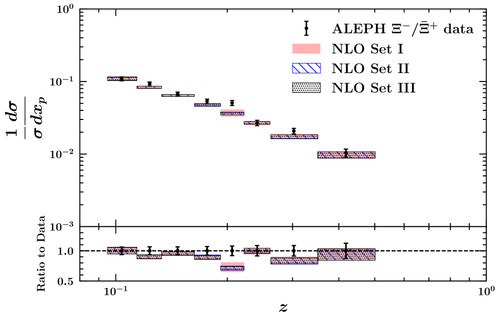
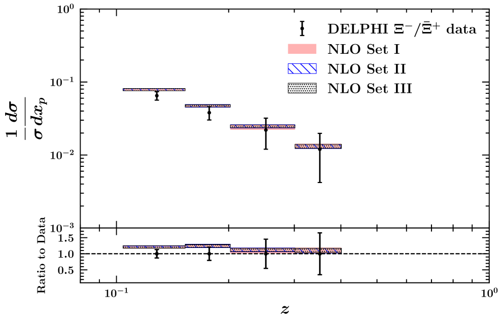
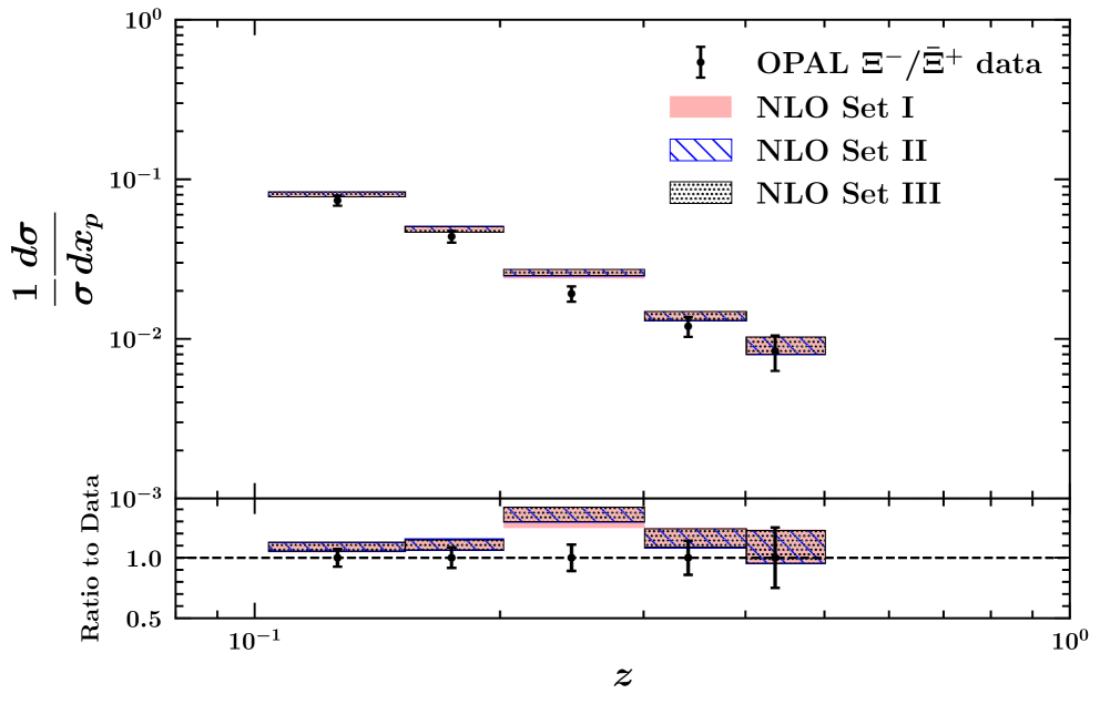
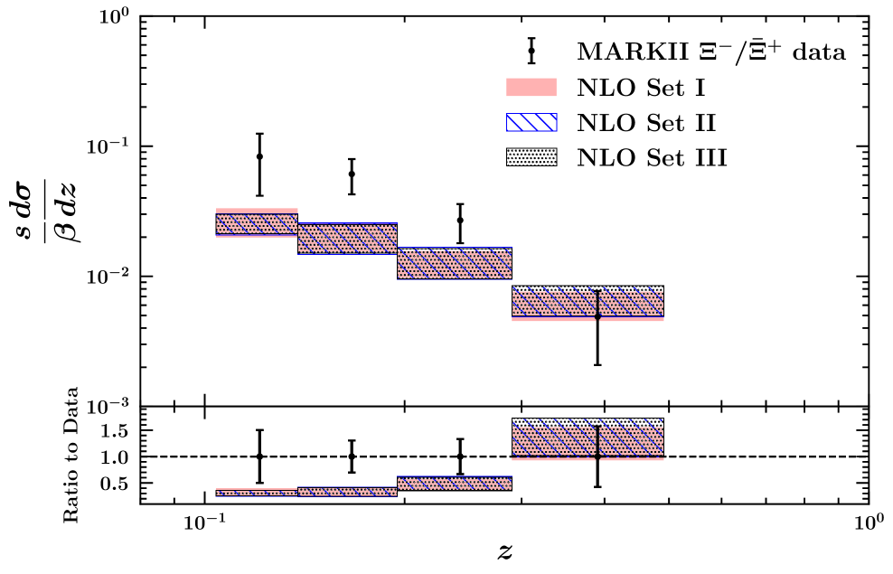
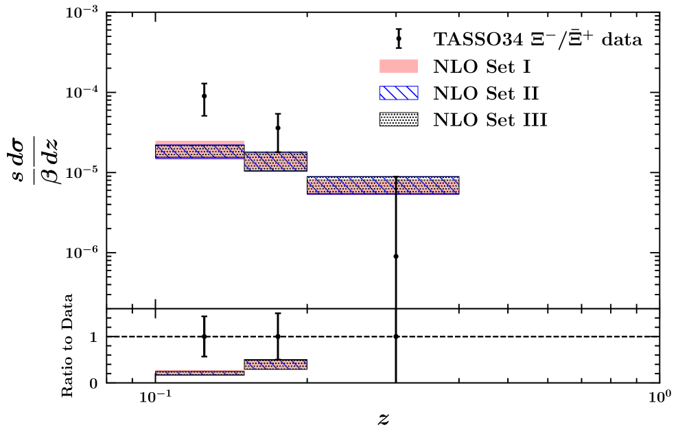
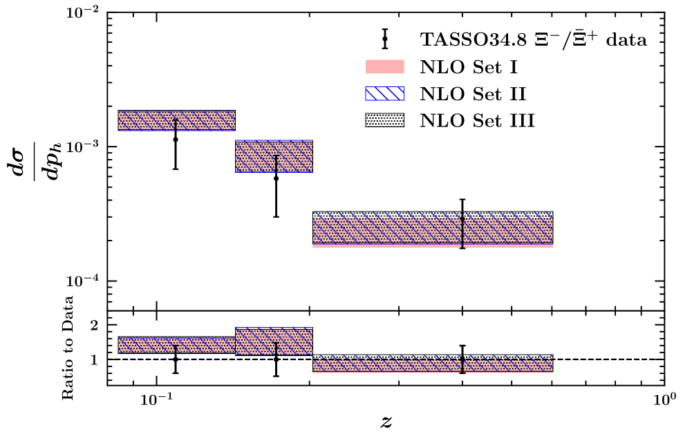
A detailed comparison of theoretical predictions obtained using the NLO FFs of set I with the SIA experimental data included in the fit is shown in Fig. 2. The data are shown as a function of $z$, limited to the range $0.1\leq z<0.5$ which corresponds to the cuts imposed in our selection of data to be fitted. We present both absolute values in upper panels and the ratios of theory prediction over data in lower panels. The results are shown for the ALEPH ALEPH:1996oqp , DELPHI DELPHI:1995dso , OPAL OPAL:1996gsw , MARKII Klein:1986ws and the TASSO Collaborations TASSO:1983qye ; TASSO:1988qlu . Overall, one can see a very good agreement between our theory predictions and the measurements for most of the data points. We observe some deviations for the MARKII and TASSO data at $\sqrt{s}=34$ GeV. These data points contribute substantially to $\chi^{2}$. For the case of ALEPH data, the agreement between theory predictions and data looks good; however, since the experimental errors are typically small their contribution to the total $\chi^{2}$ is also large.

In Table 1, introduced already above, $\chi^{2}$ values per data point for each individual dataset are shown. The total $\chi^{2}$ divided by the number of data points for each set is shown in the last row. All fits are acceptable. One can observe a slight increase of $\chi^{2}/N_{\mathrm{dat}}$ when we go from set I to sets II and III. We have included the results for sets II and III in Fig. 2. A closer inspection of these figures shows that the differences between the three sets is mainly due to two data points, one of the ALEPH and one of the OPAL data. These points appear as outliers and their contribution to the change of $\chi^{2}$ values between the three sets is particularly large.

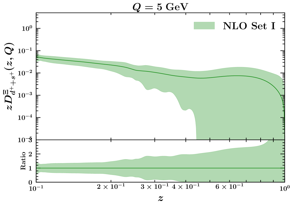
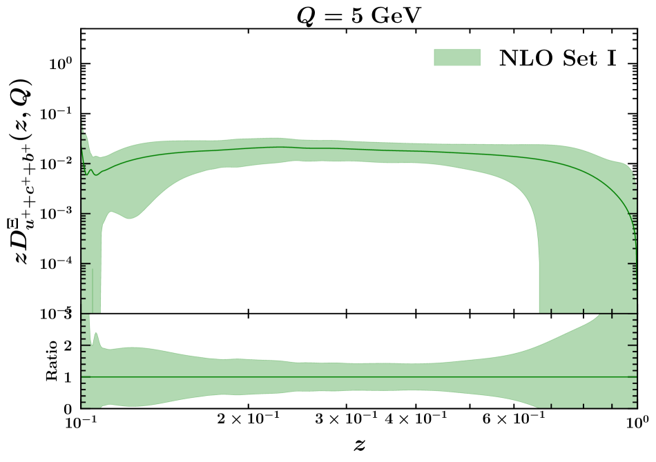
The NLO FFs of $\Xi^{-}+\bar{\Xi}^{+}$ for set I are shown in Fig. 3 together with the corresponding uncertainty bands for the two flavor combinations $d^{+}+s^{+}$ and $u^{+}+c^{+}+b^{+}$ and the gluon at the initial scale $Q_{0}=5$ GeV.

Figure 3: The flavor combinations of set I FFs at NLO for $\Xi^{-}+\bar{\Xi}^{+}$ production. Full lines describe central values, shaded areas represent corresponding uncertainty bands at the initial scale $Q_{0}=5$ GeV. The lower panels in each figure show the error bands normalized to the corresponding central values.

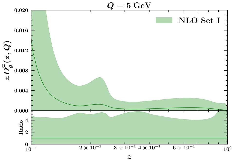
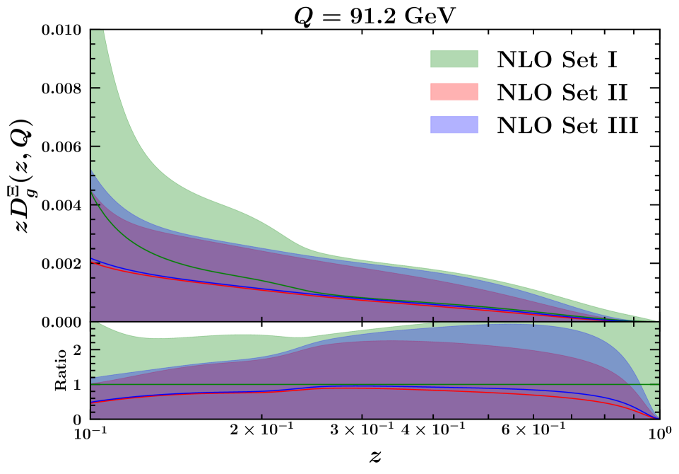
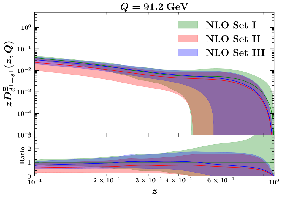
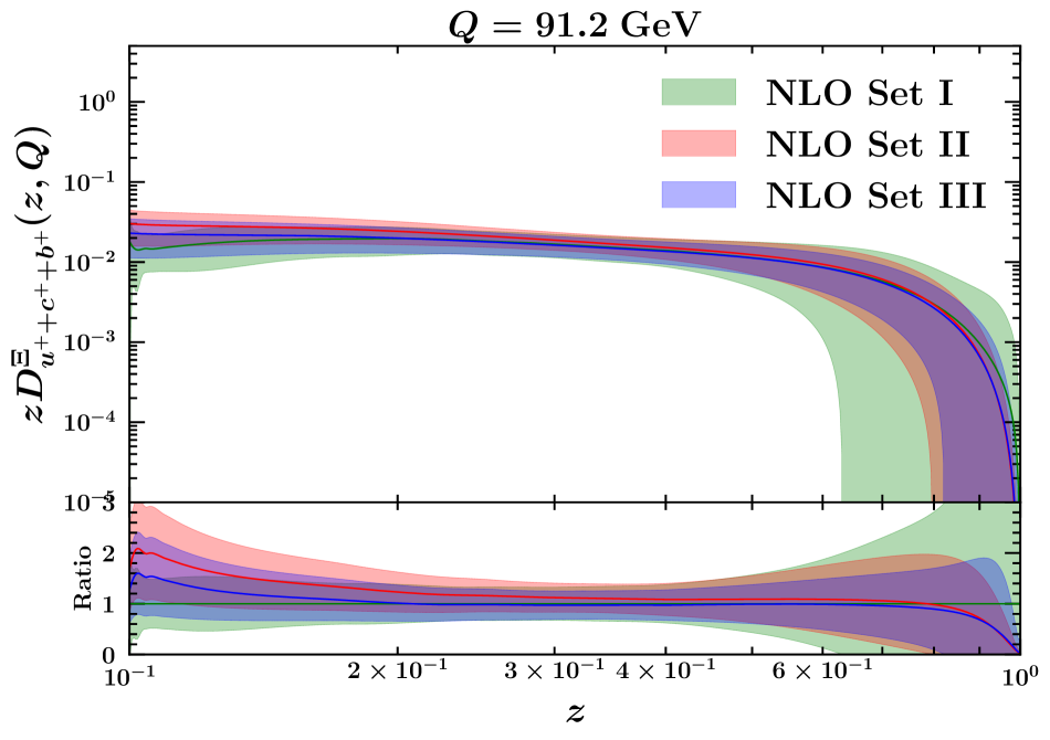
A comparison of the three sets of FF fits is shown in Fig. 4. Here we display the NLO results for the $g$, $d^{+}+s^{+}$, and $u^{+}+c^{+}+b^{+}$ FFs at the scale $Q=M_{Z}$. One can see a remarkable agreement between these different sets and the differences between the central values are almost invisible in the plots. The uncertainty bands, however, for the $d^{+}+s^{+}$ and $u^{+}+c^{+}+b^{+}$ combinations are wider for set I in the range of $z>0.4$, while these FF combinations are better constrained for set I in the small $z$-range. In fact, the available data points cover only the range $z<0.4$ and FF values above this range are the result of an extrapolation. We observe that the uncertainties of the gluon FF is larger than of the quark FFs for all fits. This was to be exptected since the SIA data are only loosely sensitive to the gluon FF.

For sets II and III, i.e. when we allow individual flavor components of the FFs to be different, we found that the central values for the same-charge combinations, i.e. $d^{+}$, $s^{+}$ and $b^{+}$ on the one hand and $u^{+}$ and $c^{+}$ on the other hand, are very similar. Therefore we do not show corresponding figures. The uncertainty bands, however, turn out to be much wider if individual components are fitted, as to be expected since the available data do not provide enough information for a separate determination of individual flavor FFs; only the corresponding sums enter the non-singlet part of the structure function $F_{2}$ in Eq. (4).

The FFs of set I contain only those flavor combinations which are needed to describe the available data, which do not distinguish light and heavy quark-initiated processes. Obviously, this is the appropriate choice to reflect the information contained in the data. Therefore we adopt set I as our baseline parametrization and present the comparison of NLO and NNLO results only for this set in the following.

Figure 4: Comparison of the FFs of set I, II and III at the scale $Q=M_{Z}=91.2$ GeV. We display the NLO results for $\Xi^{-}+\bar{\Xi}^{+}$ FFs, $zD^{\Xi^{-}+\bar{\Xi}^{+}}_{i}(z)$ ($i=g$, $d^{+}+s^{+}$, $u^{+}+c^{+}+b^{+}$).

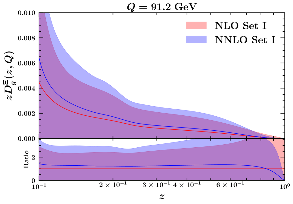
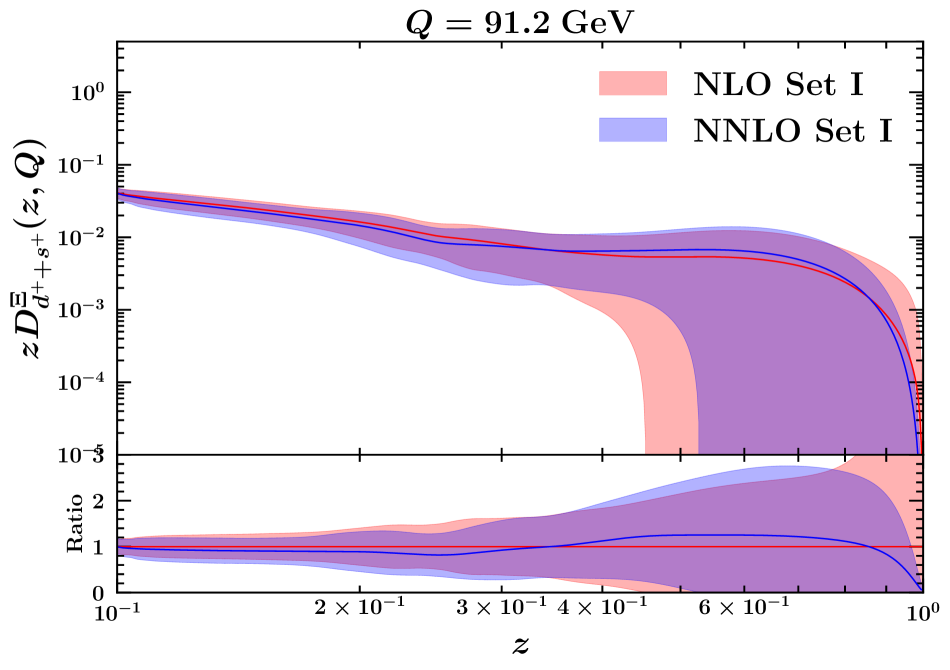
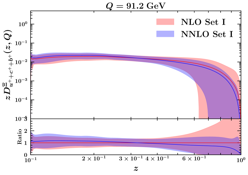
A comparison of the NLO and NNLO fits for set I is shown in Fig. 5. Central values and uncertainty bands of the FFs in Fig. 5 differ only little between the NLO and NNLO calculations. The error bands overlap everywhere. Only in the large-$z$ region, we observe some reduction of the uncertainties in the NNLO analysis. The fit quality can be judged from the $\chi^{2}$ values contained in Tab. 1. We observe that the NNLO fit yields improved values of $\chi^{2}/N_{\mathrm{dat}}$: $1.451$ for NNLO compared with $1.540$ for the NLO fit, i.e. an improvement of ${{\sim}}10\%$. This reduction of $\chi^{2}$ is shared among almost all data points except those of DELPHI and TASSO-34.8 where we observe a small increase. Overall, the inclusion of higher-order perturbative QCD corrections leads to a marginally improved set of FFs.

Figure 5: Comparison of the NLO and NNLO versions of the $\Xi^{-}+\bar{\Xi}^{+}$ FFs for the flavor combinations of set I at the scale $Q=M_{Z}$.

VII $\Xi^{-}/\bar{\Xi}^{+}$ Production at Hadron Colliders

Data for $\Xi^{-}/\bar{\Xi}^{+}$ production at hadron colliders, $p\bar{p}$ scattering at the Tevatron and $pp$ collisions at the LHC, are presently available only at very low values of the transverse momentum, $p_{T}$. Perturbative QCD is not expected to work reliably in this $p_{T}$ range and a description in a picture assuming independent parton-to-hadron fragmentation is possibly missing dominating non-perturbative effects. In order to separate such non-perturbative effects and identify possible collective phenomena, which could become important for example in the hot quark-gluon plasma in heavy-ion collisions, it will be important to compare data with predictions in a framework using FFs obtained at high energy scales and extrapolating down into the $p_{T}$ range where data already exist. On the other hand, future measurements at the LHC experiments at higher $p_{T}$ can eventually contribute to an improved determination of the $\Xi^{-}+\bar{\Xi}^{+}$ FFs.

Hadron production in $pp$ and $p\bar{p}$ collisions are sensitive to relatively large $z$ values while the available data from SIA are restricted to $z<0.5$. To some extent, our predictions are therefore based on extrapolating the $\Xi^{-}+\bar{\Xi}^{+}$ FFs into a yet unconstrained kinematic range. We have checked, however, that the hadron collider cross sections described below do have some overlap with the SIA data: about 20 % of the $pp$ and $p\bar{p}$ cross sections originate from the region with $z<0.5$.

Here we show results of the calculation of cross sections for collider experiments.

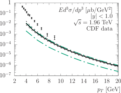
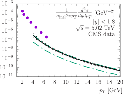
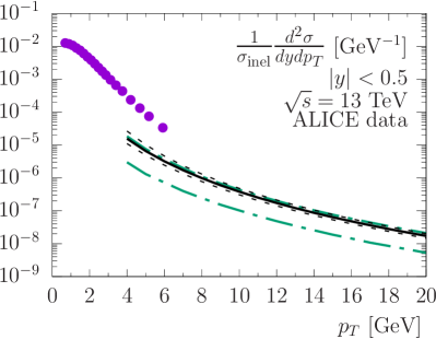
The calculation is done with code that was originally developped for the production of heavy quarks (gmvfns-3.4, described in Ref. Kniehl:2005mk ), but adapted for massless quarks for the present purpose. It is based on the results of the calculation of Ref. Aversa:1988vb which includes next-to-leading order corrections and takes into account all sub-processes with incoming and outgoing quarks and gluons. In order to connect our results with the existing data, we compare with measurements in $p\bar{p}$ collisions from CDF CDF:2011dvx at $\sqrt{s}=1.96$ TeV in the rapdity range $|y|\leq 1$, as well as in $pp$ collisions from CMS CMS:2019isl at $\sqrt{s}=5.02$ TeV, $|y|\leq 1.8$ and from ALICE ALICE:2020jsh at $\sqrt{s}=13$ TeV, $|y|\leq 0.5$. Results are shown in Fig. 6, compared with the existing data in the $p_{T}$ range up to about 6 – 8 GeV and predictions extending up to $p_{T}=20$ GeV. The default predictions, using the CT18nlo set of parton distributions from Hou:2019qau ; Hou:2019efy and the central member of the set I $\Xi^{-}+\bar{\Xi}^{+}$ FFs turn out to be considerably smaller than the data, as expected.

There are two important sources for uncertainties of the theoretical predictions: variations of the renormalization and the factorization scales, and uncertaintites due to the FF parametrization. Renormalization and factorization scales have been set equal to $p_{T}$ in our default predictions. The short-dashed lines in Fig. 6 show the error band due to variations of the renormalization scale by factors of 2 up and down. The uncertainty from variations of the factorization scales is always smaller than that due to variations of the renormalization scale. The uncertainty from the FF parametrization is, however, dominating. This is shown by the long-dash-dotted (green) lines in Fig. 6. The corresponding error band is obtained by scanning over 300 replicas of the $\Xi^{-}+\bar{\Xi}^{+}$ FFs. The predicted cross sections follow an asymmetric distribution with a mean value much smaller than the result from the central FF. The error band shown in Fig. 6 covers the $1\sigma$-range, obtained by excluding the lowest and highest $16\%$ of predicted cross section values Butterworth:2015oua . Obvsiously, with FFs from our present SHKS22 analysis, there are very large uncertainties. In turn, this means that future measurements at the LHC can be expected to provide valuable information to further constrain the FF parametrization for $\Xi^{-}+\bar{\Xi}^{+}$ hadron production. This will be particularly important for the gluon FF for which our fits with presently available data resulted in large uncertainties. In contrast to SIA data, the measurements at hadron colliders are dominated by the gluon-to-$\Xi$ FF: about 70 % of the cross section is due to this FF component. Therefore one can expect considerably reduced uncertainties of the gluon FF from future LHC data.

Figure 6: Predictions for $\Xi^{-}+\bar{\Xi}^{+}$ production at hadron colliders: CDF at the Tevatron CDF:2011dvx , CMS CMS:2019isl and ALICE ALICE:2020jsh at the LHC. In the case of CMS and ALICE, data points have been read off from the corresponding published figures and error bars are not shown since they are too small to be reliably extracted from the figures. Parton distributions from Hou:2019qau ; Hou:2019efy , set CT18nlo, were used and theory errors are shown as described in the text.

VIII Summary and Conclusions

In this paper we have introduced a new set of unpolarized FFs for $\Xi^{-}/\bar{\Xi}^{+}$ production, called SHKS22. This analysis presents the first precise determination of $\Xi^{-}/\bar{\Xi}^{+}$ fragmentation functions which include higher-order perturbative corrections at NNLO accuracy. The current analysis is based on a comprehensive dataset from single inclusive electron-positron annihilation experiments. We found that including data points in the region of $z\geq 0.1$ allows us to obtain stable fit results.

We have explored three different FF sets and parametrized them in terms of Neural Networks. This approach is expected to lead to a substantial reduction of theoretical bias in the choice of a parametrization. The parameters describing the Neural Networks are fitted to the SIA data. We have used the recent publicly available package MontBlanc to set up the parametrization of FFs, perform their evolution and calculate the SIA production cross-sections. In addition, a Monte Carlo sampling method is used to propagate the experimental uncertainties into the fitted FFs and to calculate the uncertainties for FFs and corresponding obervables.

All three sets of FFs obtained in this work describe the SIA experimental data reasonably well. Our baseline set I contains a minimal choice of parameters describing the sum of favored quark flavors $d^{+}+s^{+}$ and assumes symmetry between the disfavored quark flavors $u^{+}$, $c^{+}$ and $b^{+}$. The available data do not provide enough information to obtain precise FFs for each quark flavor separately.

Our new results provide an important ingredient needed for the calculation of theoretical predictions for the hadron production in proton-proton collisions. We have used our FFs to calculate the inclusive $\Xi^{-}+\bar{\Xi}^{+}$ baryon production in proton-proton collisions, extending the presently covered transverse momentum range of the CDF, CMS and ALICE measurements. Corresponding future measurements can then be used to extract $\Xi^{-}+\bar{\Xi}^{+}$ FFs in combination with SIA data.

The main result of this work, i.e. the $\Xi^{-}+\bar{\Xi}^{+}$ FFs, are available as grid files formatted for the LHAPDF library from the authors upon request.