Resummed lattice QCD equation of state at
finite baryon density: strangeness neutrality and beyond

Abstract

We calculate a resummed equation of state with lattice QCD simulations at imaginary chemical potentials. This work presents a generalization of the scheme introduced in Ref. [1] to the case of non-zero $\mu_{S}$, focusing on the line of strangeness neutrality. We present results up to $\mu_{B}/T\leq 3.5$ on the strangeness neutral line $\left\langle S\right\rangle=0$ in the temperature range $130\textrm{\ MeV}\leq T\leq 280$ MeV. We also extrapolate the finite baryon density equation of state to small non-zero values of the strangeness-to-baryon ratio $R=\left\langle S\right\rangle/\left\langle B\right\rangle$. We perform a continuum extrapolation using lattice simulations of the 4stout-improved staggered action with 8, 10, 12 and 16 timeslices.

I Introduction

The properties of hot and dense strongly interacting matter are the subject of many theoretical and experimental studies. At zero baryon density, first principle lattice QCD simulations showed that the transition between deconfined and confined matter is a crossover [2]. It is conjectured that the crossover line in the temperature($T$)-baryochemical potential($\mu_{B}$) plane eventually turns into a line of first order transition at a critical endpoint [3, 4, 5, 6, 7, 8].

At finite baryon density, lattice simulations face the infamous complex action or sign problem [9, 10]. Most results on finite density QCD therefore come from indirect methods, such as reweighting from zero chemical potential [11, 12, 13, 14, 15, 16, 17], Taylor expansion around zero chemical potential  [18, 19, 20, 21, 22, 23, 24, 25, 26, 27, 28, 29], or analytic continuation from imaginary chemical potentials, where the sign problem is absent [30, 31, 32, 33, 34, 35, 36, 37, 38, 39, 40, 41, 42, 43, 44, 45]. More direct simulation approaches at finite density include certain reweighting techniques [46, 17, 47], the complex Langevin equation [48, 49, 50] and methods based on Lefschetz thimbles [51, 52, 53]. Results with these more direct methods for full QCD are for the moment nonexistent (for Lefschetz thimbles) or sparse (for complex Langevin and reweighting).

Another approach to locate the critical endpoint is the analysis of data from heavy ion collision experiments. An important tool for heavy ion phenomenology is the use of relativistic hydrodynamic simulations [54, 55, 56]. These in turn need the equation of state as a theoretical input in the whole range of temperatures and densities covered by the experiment.

The equation of state at zero density (or baryochemical potential $\mu_{B}$) is known in the continuum limit from the crossover region [57, 58, 59] up to very high temperatures [60] where it can be matched with results from resummed perturbation theory [61, 62, 63].

The most straightforward way to extend the equation of state to finite chemical potentials is the use of a Taylor expansion in the chemical potential. For the pressure this reads:

$$\frac{p}{T^{4}}\left(T,\hat{\mu}_{B},\hat{\mu}_{S},\hat{\mu}_{Q}\right)=\sum_{ijk}\frac{1}{i!j!k!}\chi^{BSQ}_{ijk}\left(T\right)\hat{\mu}_{B}^{i}\hat{\mu}_{S}^{j}\hat{\mu}_{Q}^{k}\rm{,}$$ (1)

where the generalized susceptibilities are defined as

$$\chi^{BSQ}_{ijk}=\frac{\partial^{i+j+k}\left(\hat{p}\right)}{\partial^{i}\hat{\mu}_{B}\partial^{j}\hat{\mu}_{S}\partial^{k}\hat{\mu}_{Q}}$$ (2)

and the dimensionless baryochemical potential is $\hat{\mu}_{B}=\frac{\mu_{B}}{T}$, and similarly for the strangeness chemical potential $\mu_{S}$ and the electric charge chemical potential $\mu_{Q}$. The dimensionless pressure is $\hat{p}=\frac{p}{T^{4}}$. The expansion coefficients $\chi^{BSQ}_{ijk}$ can be calculated either by direct simulations at zero chemical potential or by simulations at imaginary chemical potentials, followed by a fit. The Taylor coefficients are known up to fourth order in the continuum limit [23, 24, 25]. At high temperatures, these coefficients match those calculated from resummed perturbation theory [64, 65, 66]. At finite lattice spacings, also the sixth and eights derivatives have been calculated, albeit with modest precision [43, 29].

Naive truncations of the Taylor expansion show undesirable properties above $\mu_{B}/T\gtrapprox(2-2.5)$: namely, unphysical oscillations in the equation of state. This is due to the sign structure of higher order coefficients starting from $\chi^{B}_{6}$, which is in turn caused by the $\hat{\mu}_{B}$ dependence of the crossover transition [67, 5, 68, 1, 69]. It appears that extrapolating through the crossover transition - as one is forced to do with Taylor expansions at a fixed temperature - is hard.

Figure 1: Left: The total derivative $c^{B}_{1}$ on the strangeness neutral line from our imaginary chemical potential simulations. The data points at $\mu_{B}=0$ show the second derivative $\frac{\differential^{2}\hat{p}}{\differential\hat{\mu}_{B}^{2}}$. Right: Same observables, with the temperature rescaled by a factor $1+\kappa\hat{\mu}_{B}^{2}$.

One can go beyond fixed order polynomials, by considering resummations of the Taylor series. The classic example of this is Padé resummation, which has been used also for finite density QCD [33, 70, 45, 71]. While the convergence properties of Padé approximants are in general superior to ordinary Taylor expansions, it is hard to tell which expansion will work better at the low orders of the expansion available.

A way to extend the chemical potential range accessible by indirect methods already at low orders of the approximation is the use of a physically motivated extrapolation scheme. Recently, in Ref. [1] the authors of this paper introduced exactly such a scheme. It was motivated by an important finding in recent studies of the crossover region at imaginary chemical potentials: the existence of an approximate scaling variable $T(1+\kappa\left(1+\kappa\hat{\mu}_{B}^{2}\right)$, where $T$ is the temperature, and $\mu_{B}$ the baryochemical potential. In this variable, many observables - such as the chiral condensate or the baryon number-to-chemical potential ratio $\chi^{B}_{1}/\mu_{B}$ - when measured at different fixed values of $\operatorname{Im}\mu_{B}/T$ as a function of temperature, collapse to the same curve [44, 1]. Up to $\mu_{B}/T=1.5$ the existence of an approximate scaling variable has also been confirmed directly at a real baryochemical potential, by reweighting from the sign quenched ensemble [47].

One might suspect that the existence of such an approximate scaling variable is ultimately related to criticality in the two-flavour chiral limit of QCD [72, 73]. If the universal contribution to the equation of state is large, one expects a single scaling variable - which is a combination of the quark mass, the temperature and the chemical potential - to govern most thermodynamic observables. If in the low chemical potential region the strength of the transition is ultimately governed by the quark mass, one expects curves sensitive to criticality to not change shape significantly at small chemical potentials. This is also consistent with the observation that the width of the crossover transition is, to a good approximation, constant at small $\mu_{B}$ [36, 44].

Based on these observations, one can define the systematically improvable ansatz:

$$F(T,\hat{\mu}_{B})=F(T(1+\kappa^{F}_{2}(T)\hat{\mu}_{B}^{2}+\kappa^{F}_{4}(T)\hat{\mu}_{B}^{4}+\dots),0)\rm{,}$$ (3)

where $F$ is some observable of interest, of sigmoid shape in the temperature, such as $\chi^{B}_{1}/\hat{\mu}_{B}$. The superscripts on the $\kappa^{F}_{n}$ denote that the expansion coefficients are different for different observables. The approximate constant strength of the crossover transition at small chemical potentials is manifest in the approximate temperature independence of the coefficient $\kappa_{2}(T)$ in the crossover region. A strengthening or weakening of the transition at larger chemical potentials could in turn manifest itself in a non-trivial temperature dependence of the higher order expansion coefficients $\kappa_{n}$ in the crossover region.

While in our previous study in Ref. [1] we showed the QCD equation of state up to $\mu_{B}/T=3.5$ for the simplest case of $\mu_{S}=\mu_{Q}=0$, for the phenomenologically more relevant strangeness neutral line $\chi^{S}_{1}=0$, the equation of state from first principle calculations is still only available as a fixed order Taylor expansion at fixed $T$, and it therefore covers a rather limited range in the chemical potentials, due to the aforementioned unphysical oscillations.

Here, we extend our previous investigations using our novel resummation scheme, conducted at zero strangeness chemical potential $\mu_{S}=0$ in Ref. [1] to the strangeness neutral line, and present results up to $\mu_{B}/T=3.5$ in this setting. This equation of state can be used in those hydrodynamic simulations where local strangeness neutrality is enforced everywhere.

We also introduce a further component of the resummation scheme - the Stefan-Boltzmann correction discussed in the next section. This will improve the convergence of our ansatz at high temperatures - where the aforementioned approximate scaling does not hold.

Finally, we go beyond strangeness neutrality by calculating - at finite real $\mu_{B}$ - the expansion coefficients needed to calculate the equation of state at small values of the strangeness-to-baryon number ratio:

$$R\equiv\frac{\left\langle S\right\rangle}{\left\langle B\right\rangle}=\frac{\chi^{S}_{1}}{\chi^{B}_{1}}\rm{.}$$ (4)

This allows one to relax the condition of local strangeness neutrality in hydrodynamic simulations. This is necessary, as in a heavy ion collision, only global strangeness neutrality is guaranteed, and local charge fluctuations can be large.

The structure of the paper is as follows. In Sec. II we briefly describe the strangeness neutrality condition. In Sec. III. we formally define our extrapolation ansatz on the strangeness neutral line, including the Stefan-Boltzmann improvement. In Sec. IV we describe our method to determine the extrapolation coefficients. In Sec. V we use the coefficients determined in Sec. IV to calculate thermodynamics at finite real chemical potentials both on the strangeness neutrality line and its vicinity.

II Strangeness neutrality

When enforcing strangeness neutrality, two sets of conditions are widely used in the literature. In the first, one sets $\mu_{Q}=0$ and defines a curve in the $\mu_{B}-\mu_{S}$ plane by the condition $\chi^{S}_{1}=0$. By differentiation, this implies:

$$\frac{\differential\mu_{S}}{\differential\mu_{B}}=-\frac{\chi^{BS}_{11}}{\chi^{S}_{2}}\rm{.}$$ (5)

On this line, total derivatives with respect to the baryochemical potential read

$$\frac{\differential}{\differential\hat{\mu}_{B}}=\frac{\partial}{\partial\hat{\mu}_{B}}+\frac{\differential\hat{\mu}_{S}}{\differential\hat{\mu}_{B}}\frac{\partial}{\partial\hat{\mu}_{S}}=\frac{\partial}{\partial\hat{\mu}_{B}}-\frac{\chi^{BS}_{11}}{\chi^{S}_{2}}\frac{\partial}{\partial\hat{\mu}_{S}}\rm{.}$$ (6)

We denote the total derivatives of the dimensionless pressure with respect to the baryochemical potential along the line $\mu_{Q}=0$ and $\chi^{S}_{1}=0$ as:

$$c^{B}_{n}(T,\hat{\mu}_{B})\equiv\frac{\differential^{n}\hat{p}(T,\hat{\mu}_{B})}{\differential\hat{\mu}_{B}^{n}}\Bigg{|}_{\begin{subarray}{c}\mu_{Q}=0\\ \chi^{S}_{1}=0\end{subarray}}\rm{.}$$ (7)

In this scheme, the leading coefficient

$$c^{B}_{1}(T,\hat{\mu}_{B})=\chi^{B}_{1}-\frac{\chi^{BS}_{11}}{\chi^{S}_{2}}\chi^{S}_{1}=\chi^{B}_{1}$$ (8)

gives the net baryon density.

Since a vanishing electric charge chemical potential is equivalent to zero isospin, this condition is equivalent to $\chi^{Q}_{1}=0.5\chi^{B}_{1}$. While this is a much better approximation for the conditions of a heavy ion collision than simply taking $\mu_{S}=\mu_{Q}=0$, there is a further correction which can be taken into account: the slight isospin imbalance of the colliding nuclei (typically lead or gold). This amounts to the two constraints $\chi^{S}_{1}=0$ and $0.4\chi^{B}_{1}=\chi^{Q}_{1}$, which define a curve in the $\mu_{B}-\mu_{S}-\mu_{Q}$ space. Along this curve the total derivatives are:

$$\frac{\differential}{\differential\hat{\mu}_{B}}=\frac{\partial}{\partial\hat{\mu}_{B}}+\frac{\differential\hat{\mu}_{S}}{\differential\hat{\mu}_{B}}\frac{\partial}{\partial\hat{\mu}_{S}}+\frac{\differential\hat{\mu}_{Q}}{\differential\hat{\mu}_{B}}\frac{\partial}{\partial\hat{\mu}_{Q}}\rm{,}$$ (9)

where $\frac{\differential\hat{\mu}_{S}}{\differential\hat{\mu}_{B}}$ and $\frac{\differential\hat{\mu}_{Q}}{\differential\hat{\mu}_{B}}$ are given by the solution of the constraints:

$$\chi^{BS}_{11} +\chi^{SQ}_{11}\frac{\differential\hat{\mu}_{Q}}{\differential\hat{\mu}_{B}}+\chi^{S}_{2}\frac{\differential\hat{\mu}_{S}}{\differential\hat{\mu}_{B}}=0$$ (10)

$$\chi^{BQ}_{11} +\chi^{SQ}_{11}\frac{\differential\hat{\mu}_{S}}{\differential\hat{\mu}_{B}}+\chi^{Q}_{2}\frac{\differential\hat{\mu}_{Q}}{\differential\hat{\mu}_{B}}=$$

$$0.4\left(\chi^{B}_{2}+\chi^{BS}_{11}\frac{\differential\hat{\mu}_{S}}{\differential\hat{\mu}_{B}}+\chi^{BQ}_{11}\frac{\differential\hat{\mu}_{Q}}{\differential\hat{\mu}_{B}}\right)$$

Along this line, total derivatives will be denoted:

$$d^{B}_{n}(T,\hat{\mu}_{B})\equiv\frac{\differential^{n}\hat{p}(T,\hat{\mu}_{B})}{\differential\hat{\mu}_{B}^{n}}\Bigg{|}_{\begin{subarray}{c}\chi^{Q}_{1}=0.4\chi^{B}_{1}\\ \chi^{S}_{1}=0\end{subarray}}\rm{.}$$ (11)

For simplicity, through most of this manuscript, we will use the first set of conditions with $\mu_{Q}=0$. In Sec. IV.2., we will consider the difference between the two schemes in the leading order of the Taylor expansion - i.e. we will calculate $c^{B}_{2}(T,0)$ and $d^{B}_{2}(T,0)$ and their temperature derivatives, at which point we will also discuss the rationale for our choice of the first setting with $\mu_{Q}=0$.

Figure 2: Left: The scaled total derivative $c^{B}_{1}/\hat{\mu}_{B}$ on the strangeness neutral line from our imaginary chemical potential simulations, divided by its chemical potential dependent Stefan-Boltzmann limit. The data points at $\mu_{B}=0$ show the second derivative $c^{B}_{2}$ divided by its Stefan-Boltzmann limit. Right: Same observables, with the temperature rescaled by a factor $1+\lambda\hat{\mu}_{B}^{2}$.

III The extrapolation scheme

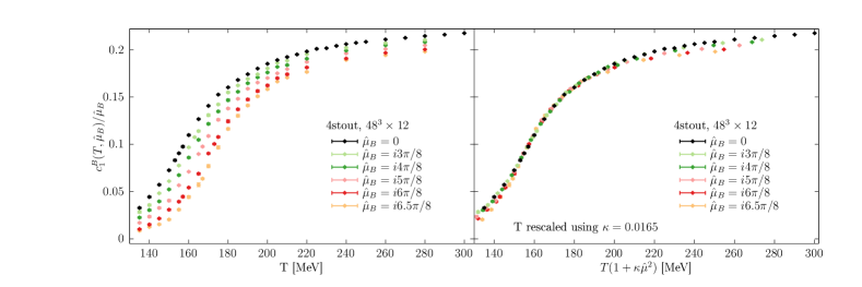
Before describing our improved extrapolation ansatz, we note that the ansatz given by Eq. (3), introduced in [1] for $\mu_{S}=0$, would also work at strangeness neutrality. The existence of the approximate scaling variable on the strangeness neutral line is shown in Fig. 1 for the quantity $c^{B}_{1}/\mu_{B}$, where on the left panel we show the data points of our simulations for a $48^{3}\times 12$ lattice, while on the right panel we show the same data points as a function of a rescaled temperature $T(1+\kappa\hat{\mu}^{2})$. Notice that the collapse plot with a constant $\kappa$ does not work quite as well at high temperatures. Indeed, one does not expect an approximate scaling variable outside the crossover range. Our scheme can still incorporate this behavior by the temperature dependence of the $\kappa_{n}$ coefficients. In fact, with the ansatz given by Eq. (3) the coefficient $\kappa_{2}$ grows at high temperatures (see later).

One shortcoming of this scheme is that the region of applicability is restricted by the Stefan-Boltzmann limit of the right hand side of Eq. (3). When the quantity $F(T,\hat{\mu}_{B})$ becomes larger than its infinite temperature limit at $\mu_{B}=0$, the ansatz in Eq. (3) must break down. It is easy to address this shortcoming however, using the scheme only for observables $F$ that have an infinite temperature limit that is independent of $\hat{\mu}_{B}$. Given an observable that does not possess this property, one can easily construct another observable, by simply dividing by its own Stefan-Boltzmann limit:

$$F(T,\hat{\mu}_{B})\to\frac{F(T,\hat{\mu}_{B})}{\overline{F}(\hat{\mu}_{B})}\rm{,}$$ (12)

where the Stefan-Boltzmann limits  are denoted by

$$\overline{F}(\hat{\mu}_{B}) =\lim_{T\to\infty}F(T,\hat{\mu}_{B})\rm{.}$$ (13)

By construction, the ratio on the right hand side of Eq. (13) has an infinite temperature limit equal to one, at all values of $\hat{\mu}_{B}$. By using the ansatz from Eq. (3) on this Stefan-Boltzmann corrected observable, we arrive at our new scheme, given by

$$\frac{F(T,\hat{\mu}_{B})}{\overline{F}(\hat{\mu}_{B})}=\frac{F(T_{F}^{\prime},0)}{\overline{F}(0)}\rm{,}$$ (14)

where the temperature on the right hand side is expanded as

$$T_{F}^{\prime}=T\left(1+\lambda^{F}_{2}(T)\hat{\mu}_{B}^{2}+\lambda^{F}_{4}(T)\hat{\mu}_{B}^{4}+\dots\right)\rm{.}$$ (15)

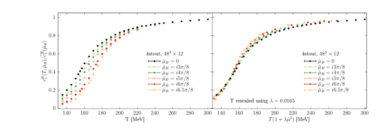
As is shown in Fig. 2, this Stefan-Boltzmann correction does not spoil the collapse plot in the approximate scaling variable, meaning that the fast convergence of the scheme in the crossover region is maintained, with a $\lambda_{2}(T)$ coefficient that is approximately constant in the crossover range. The limitation at high temperature is however removed. Furthermore, as can be seen on the left panel of Fig. 2, the coefficients $\lambda_{n}$ must go to zero at high temperatures, as the data points for the different imaginary chemical potentials almost overlap. This is in contrast to the scheme of Eq. (3), where $\kappa_{2}$ grows at high temperatures.

For any finite order in the expansion in the $\lambda_{n}$, Eq. (14) generates an infinite number of terms in the Taylor expansion of the quantity $F$, thus the ansatz achieves a particular resummation of the Taylor expansion. As discussed in the introduction, this resummation is expected to converge fast in the crossover region, where the strength of the transition stays approximately constant.

In this work, we will consider three different observables $F$. First, we consider the normalized net baryon density $F=c^{B}_{1}/\hat{\mu}_{B}$. By noticing that $\lim_{\hat{\mu}_{B}\to 0}\frac{c^{B}_{1}(T,\hat{\mu}_{B})}{\hat{\mu}_{B}}=c^{B}_{2}(T,0)$, Eq. (14) becomes:

$$\frac{c^{B}_{1}(T,\hat{\mu}_{B})}{\overline{c^{B}_{1}}(\hat{\mu}_{B})}=\frac{c^{B}_{2}(T_{BB}^{\prime},0)}{\overline{c^{B}_{2}}(0)}\rm{,}$$ (16)

where the infinite temperature limits of $c^{B}_{1}$ and $c^{B}_{2}$ are denoted $\overline{c^{B}_{1}}$ and $\overline{c^{B}_{2}}$ respectively, and

$$T_{BB}^{\prime}\equiv T(1+\lambda_{2}^{BB}(T)\hat{\mu}_{B}^{2}+\lambda_{4}^{BB}(T)\hat{\mu}_{B}^{4}+\dots)\rm{.}$$ (17)

The Stefan-Boltzmann limits are easily obtained:

$$\overline{c^{B}_{1}}(\hat{\mu}_{B}) = \hat{\mu}_{B}\overline{c^{B}_{2}}(0)+\hat{\mu}_{B}^{3}\overline{c^{B}_{4}}(0)$$

$$\overline{c^{B}_{2}}(0) = \frac{2}{9}\qquad\overline{c^{B}_{4}}(0)=\frac{4}{27\pi^{2}}$$ (18)

The $c_{2}^{B}(T,0)$ function at $\mu_{B}=0$ together with the temperature-dependent coefficients in Eq. (17) are sufficient to extrapolate the strangeness-neutral equation of state to finite baryon density as we will show in Section. V.

Second, we will consider the normalized strangeness chemical potential that is needed to realize the $\chi^{S}_{1}\equiv 0$ condition in a grand canonical ensemble: $F=\rm{M}(T,\hat{\mu}_{B})\equiv\frac{\hat{\mu}_{S}}{\hat{\mu}_{B}}\left(T,\hat{\mu}_{B}\right)$. Since

$$\lim_{\hat{\mu}_{B}\to 0}\rm{M}(T,\hat{\mu}_{B})=-\frac{\chi^{BS}_{11}(T,0)}{\chi^{S}_{2}(T,0)}\equiv\rm{M}(T,0)\rm{,}$$ (19)

Eq. (14) becomes:

$$\frac{\rm{M}(T,\hat{\mu}_{B})}{\overline{\rm{M}}(\hat{\mu}_{B})}=\frac{\rm{M}(T_{BS}^{\prime},0)}{\overline{\rm{M}}(0)}\rm{,}$$ (20)

with the Stefan Boltzmann limit $\overline{\rm{M}}(\hat{\mu}_{B})=\lim_{T\to\infty}\rm{M}(T,\hat{\mu}_{B})$ and

$$T_{BS}^{\prime}=T(1+\lambda_{2}^{BS}(T)\hat{\mu}_{B}^{2}+\lambda_{4}^{BS}(T)\hat{\mu}_{B}^{4}+\dots)\rm{.}$$ (21)

Finally, we will also consider $F=\chi^{S}_{2}$, and denote its Stefan-Boltzmann limit by $\overline{\chi^{S}_{2}}$. For this observable, Eq. (14) reads:

$$\frac{\chi^{S}_{2}(T,\hat{\mu}_{B})}{\overline{\chi^{S}_{2}}(\hat{\mu}_{B})}=\frac{\chi^{S}_{2}(T_{SS}^{\prime},0)}{\overline{\chi^{S}_{2}}(0)}\rm{,}$$ (22)

where

$$T_{SS}^{\prime}=T(1+\lambda_{2}^{SS}(T)\hat{\mu}_{B}^{2}+\lambda_{4}^{SS}(T)\hat{\mu}_{B}^{4}+\dots)\rm{.}$$ (23)

Note that, at strangeness neutrality, the Stefan-Boltzmann limits of $\rm{M}$ and $\chi^{S}_{2}$ are independent of $\hat{\mu}_{B}$,

$$\overline{\rm{M}}(\hat{\mu}_{B})=\hat{\mu}_{B}\overline{\rm{M}}(0)\,,\qquad\overline{\chi^{S}_{2}}(\hat{\mu}_{B})=1\,,$$ (24)

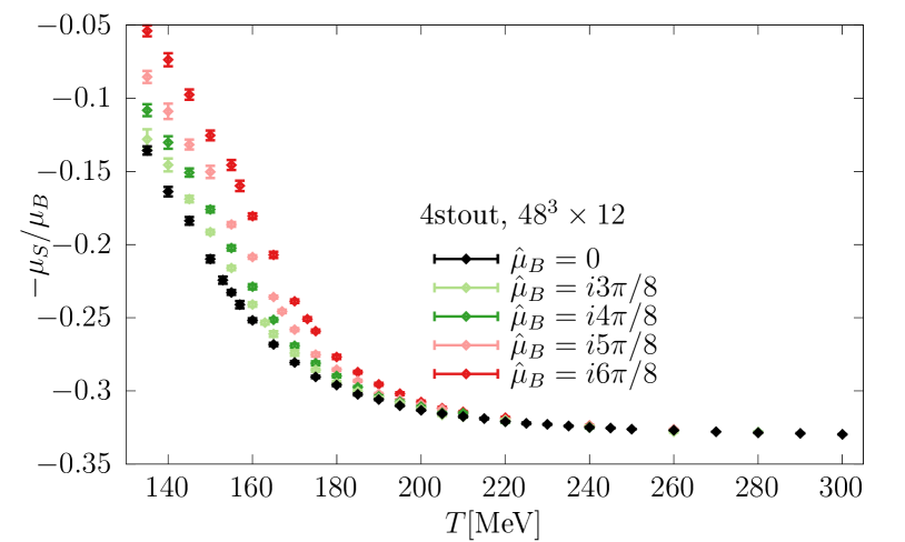
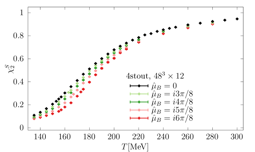
thus $\kappa_{n}^{BS}=\lambda_{n}^{BS}$ and $\kappa_{n}^{SS}=\lambda_{n}^{SS}$. This concludes the definition of our scheme for all observables of interest. We show the lattice data for $\rm{M}$ and $\chi^{S}_{2}$ on our $48^{3}\times 12$ ensembles in Figure 3.

Figure 3: The strangeness to baryon chemical potential ratio (upper panel) and the strangeness susceptibility (lower panel) at simulated imaginary baryochemical potentials on our $48^{3}\times 12$ ensembles.

Figure 4: The $\kappa_{2}\equiv\kappa^{BB}_{2}$ coefficients obtained in the scheme of Eq. (3) without the Stefan-Boltzmann correction (in red), compared to the coefficients $\lambda_{2}\equiv\lambda^{BB}_{2}$ obtained in the scheme of Eq. (14) with the Stefan-Boltzmann correction (in black) on our $48^{3}\times 12$ lattices.

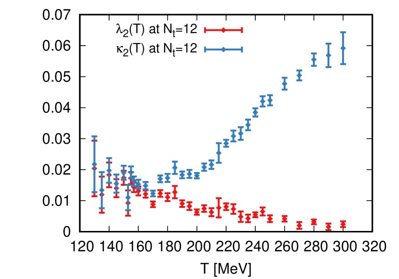
Finally, in order to illustrate the advantageous properties of the Stefan-Boltzmann correction mentioned above, we compare the $\kappa^{BB}_{2}$ and $\lambda^{BB}_{2}$ coefficients obtained without and with the Stefan-Boltzmann correction respectively, in Fig.  4 for our $48^{3}\times 12$ lattices.

IV Determination of the expansion coefficients

IV.1 Lattice setup

We perform simulations with $N_{f}=2+1+1$ dynamical quark flavours, with physical light, strange and charm quark masses. We use staggered fermions with fat links constructed with 4 steps of stout smearing [75] with the smearing parameter $\rho=0.125$ and a tree-level Symanzik-improved gauge action. This discretization of the QCD action was first used in Ref. [23], where information about the line of constant physics can be found. For the scale setting we use either the pion decay constant $f_{\pi}=130.41$MeV [76], or the Wilson flow based $w_{0}=0.1725$fm scale introduced in Ref. [77]. Taking into account the difference between the two scale settings is part of our systematic error analysis. We use lattices of temporal extent $N_{\tau}=8,10,12$ ad $16$ to perform a continuum limit. The spatial volume is given by the aspect ratio of $LT=4$. We performed simulations for imaginary baryochemical potentials given by $\operatorname{Im}\hat{\mu}_{B}\frac{8}{\pi}=0,3,4,5,6,6.5$. In addition, for the $N_{\tau}=12$ lattices we also have data at $\operatorname{Im}\hat{\mu}_{B}\frac{8}{\pi}=5.5$. Strangeness neutrality was enforced on our imaginary chemical potential ensembles via the procedure discussed in Ref. [44].

IV.2 $c^{B}_{2}$, $d^{B}_{2}$ and their $T$ derivative at $\mu_{B}=0$

In order to determine thermodynamics at finite real chemical potentials, the right hand side of Eq. (16), i.e. $c^{2}_{B}(T,0)$ must be known. For some quantities, like the entropy, its temperature derivative is also needed. We describe the determination of this quantity and its derivative here.

Given the second order quark number susceptibilities at vanishing chemical potentials, one can express $c^{B}_{2}(T,0)$ as

$$c^{B}_{2}(T,0)=\chi^{B}_{2}-\frac{\left(\chi^{BS}_{11}\right)^{2}}{\chi^{S}_{2}}\rm{,}$$ (25)

which we continuum extrapolate using our $N_{\tau}=10,12$ and $16$ lattices (for $c^{B}_{2}(T)$ and $\rm{M}(T)$) or $N_{\tau}=12,16$ and $20$ (for $\chi^{S}_{2}(T)$), using a tree level improvement when applicable [23]. For the calculation of the temperature derivative we use the same procedure as in Ref. [1]. A procedure which we also describe here, to make the manuscript self contained.

The derivatives are obtained by fitting the data with suitable ansätze, which address then differentiated. We first divide the temperature range into two parts: the crossover region and the high temperature region. For the low temperature region we interpolate $c^{B}_{2}$ with basis splines with nodes points in the range $T\in\left[130\rm{MeV},300\rm{MeV}\right]$. The splines are cubic. We perform a joint fit of the splines in temperature and in $1/N_{\tau}^{2}$. The ansatz reads:

$$c^{2}_{B}(T,0)=\sum_{i=1}^{n}\alpha_{i}b_{i}(T)+\frac{1}{N_{\tau}^{2}}\sum_{i=1}^{n}\beta_{i}b_{i}(T).$$ (26)

Here, the basis splines satisfy $b_{i}(T_{j})=\delta_{ij}$ where the $T_{j}$ with $1\leq j\leq n$ are the node points for the given basis function. To estimate the systematics of the interpolation, we combine results from four sets of the node points $T_{j}$. The systematic error estimation also includes the difference between the $f_{\pi}$ and $w_{0}$ bases scale setting. We only kept fits with a $Q$ value higher than 5%, these then we combined with uniform weights. The $c^{B}_{2}(T)$ and $\rm{M}(T)$ fits were constrained at temperatures below $130$MeV to match predictions from the hadron resonance gas (HRG) model.

Figure 5: $c^{B}_{2}(T,\hat{\mu}_{B}=0)$, $d^{B}_{2}(T,\hat{\mu}_{B}=0)$ and their logarithmic temperature derivatives in the continuum limit, as extrapolated from our $N_{\tau}=10,12$ and $16$ lattices.

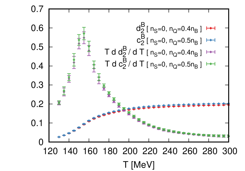
In the large temperature range we performed a polynomial fit in $1/T$. The known Stefan-Boltzmann limit is not enforced in the constant term of the polynomial. Hence, the fitted value of the constant is not equal to the known infinite temperature limit, and our fit only allows for interpolation in the range where we have lattice data. The region where the two ansätze overlap give consistent results in the temperature range between $200$MeV and $280$MeV for both $c^{B}_{2}$ and its $T$ derivative. In the final result, we simply concatenate the two results at $T=250$MeV. Final results for $c^{B}_{2}(T,0)$ and its logarithmic temperature derivative are shown in Fig. 5.

We also performed the same analysis for $d^{B}_{2}(T,0)$, corresponding to $\chi_{Q}=0.4\chi_{B}$. The results for this quantity and its temperature derivative are also shown in Fig. 5. At large temperatures, there is a small but statistically significant difference between $d^{B}_{2}$ and $c^{B}_{2}$. The difference of these Taylor coefficients leads to a small difference between the leading order chemical potential dependence in these two cases for high temperatures. The next corrections, corresponding to the $\lambda^{BB}_{n}$ coefficients of our resummation scheme, would probably also slightly differ in the two cases, but our lattice results are not yet precise enough to detect this difference. Therefore, we go on with the $\mu_{Q}=0$ setting for simplicity.

Figure 6: The determination of the rescaled temperatures $T_{BB}^{\prime}$ by spline fits to the data at zero and imaginary baryochemical potential. Solid lines represent the spline fits to the lattice data, while transparent lines represent the shifts $\Delta T_{BB}=T^{\prime}_{BB}-T$extracted from the splines.

Figure 7: Expansion coefficients $\lambda^{BB}_{n}$ (top panel), $\lambda^{BS}_{n}$ (middle panel) and $\lambda^{SS}_{n}$ (bottom panel) in the continuum. Also shown are the fits used to estimate the temperature derivative of these coefficients, as well as predictions of the hadron resonance gas model, which we use to constrain the fits at low temperatures.

IV.3 Analysis of the coefficients $\lambda_{2}$ and $\lambda_{4}$

The analysis proceeds in the same way for all three observables we study. Denoting by $A$ either one of the observables $c^{B}_{1}$, $\rm{M}=\frac{\mu_{S}}{\mu_{B}}$ and $\chi^{S}_{2}$ and calling $B$ one of $c^{B}_{2}$, $-\frac{\chi^{BS}_{11}}{\chi^{S}_{2}}$ or $\chi^{S}_{2}$ respectively, and denoting the corresponding Stefan-Boltzmann corrected observables by $\tilde{A}=A/\overline{A}$ and $\tilde{B}=B/\overline{B}$ respectively, our extrapolation ansatz is defined as

$$\tilde{A}(T,\hat{\mu}_{B})=\tilde{B}(T^{\prime},0)\rm{.}$$ (27)

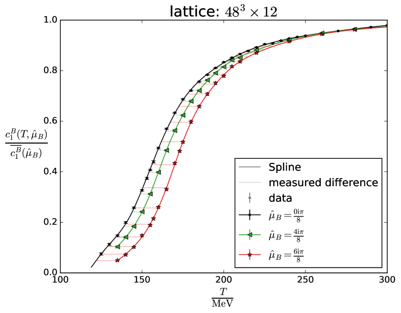
In the first step of the analysis, a spline interpolation is performed for $\tilde{A}$ at finite imaginary $\mu_{B}$ and for $\tilde{B}$ at $\mu_{B}=0$. In the second step, these splines are used for each imaginary $\hat{\mu}_{B}$, and several values of $\tilde{A}(T,\hat{\mu}_{B})$ to determine a $T^{\prime}$ that solves Eq. (27). This procedure is illustrated in Fig. 6. After finding the values of $T^{\prime}$, we construct the quantity

$$\Pi(T,\hat{\mu}_{B},N_{\tau})=\frac{T^{\prime}(T,\hat{\mu}_{B},N)-T}{T\hat{\mu}_{B}}\rm{.}$$ (28)

As $\lim_{\hat{\mu}_{B}\to 0}\Pi=\lambda_{2}^{ij}$, with $ij$ being either one of $BB$, $BS$ or $SS$, we can also add a data point at $\mu_{B}=0$ by utilizing the formulas connecting the ordinary Taylor coefficients defined in Eq. (2) to the $\lambda_{n}$ coefficients defined in Sec. III. For reference, these formulas are listed in the Appendix. In the third step, we fit the quantity $\Pi(T,\hat{\mu}_{B},N_{\tau})$ with an ansatz that is linear in $1/N_{\tau}^{2}$ and either linear or parabolic in $\mu_{B}^{2}$ - i.e.:

$$\Pi(T,\hat{\mu}_{B},N_{\tau}) =\lambda^{A}_{2}+\lambda^{A}_{4}\hat{\mu}_{B}^{2}+\lambda^{A}_{6}\hat{\mu}_{B}^{4}$$ (29)

$$+\frac{1}{N_{\tau}^{2}}\left(\alpha^{A}+\beta^{A}\hat{\mu}_{B}^{2}+\gamma^{A}\hat{\mu}_{B}^{4}\right)$$

where we either fix $\lambda^{A}_{6}=\gamma^{A}=0$ or leave both as free parameters in the fit.

Systematic errors were estimated by combining several fits with uniform weights, as long as their $Q$ value is above $1\%$. The different choices in the analysis procedure include:

• 3 different sets of spline node points at $\mu_{B}$=0

• 2 different sets of spline node points at finite imaginary $\mu_{B}$

• $w_{0}$ or $f_{\pi}$ based scale setting

• 2 different chemical potential ranges in the global fit: $\hat{\mu}_{B}\leq 5.5$ or $\hat{\mu}_{B}\leq 6.5$

• 2 functions for the chemical potential dependence of the global fit: linear or parabola

• including the coarsest lattice, $N_{\tau}=8$, or not, in the continuum extrapolation.

This amounts to a total of $96=3\times 2^{5}$ fits entering the systematic error estimation.

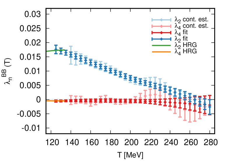
For calculating certain thermodynamic quantities at finite chemical potential, such as the entropy, the temperature derivative of the $\lambda_{n}$ coefficients is also needed. To estimate these derivatives we perform an uncorrelated fit of the obtained expansion coefficients with a fourth order polynomial ansatz for the $\lambda^{ij}_{2}$ and a second order polynomial ansatz for the $\lambda^{ij}_{4}$. For the lower end of our temperature range, the fits are constrained to the values predicted by the hadron resonance gas model. In order not to dominate the fits, the hadron resonance gas predictions are taken to have error bars of the same size as our lattice data. The expansion coefficients and the fits used to estimate their temperature derivative are shown in Fig. 7. All of the $\lambda_{2}$ coefficients are approximately constant in the crossover range, as is expected from the existence of the approximate scaling variable, discussed in the introduction. With the exception of $\lambda^{SS}_{2}$, the $\lambda_{2}$ coefficients all go to zero within error bars at higher end of our temperature range, as was anticipated in the discussion of Fig. 2. The $\lambda^{SS}_{2}$ is still non-zero, as the strangeness susceptibility $\chi^{S}_{2}$ tends to its Stefan-Boltzmann more slowly, due to the larger strange quark mass.

V Thermodynamics at real $\mu_{B}$

V.1 Thermodynamics on the $\chi^{S}_{1}=0$ line

Figure 8: The dimensionless baryon density (top left panel), pressure (top right panel), entropy (middle left panel), energy density (middle right panel), strangeness chemical potential-to-baryochemical potential ratio (bottom left panel) and strangeness susceptibility (bottom right panel) as functions of temperature at different values of the real chemical potential. The solid lines always show the predictions of the hadron resonance gas model for the corresponding temperature.

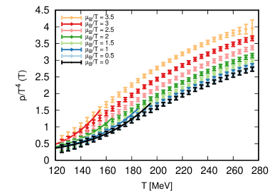
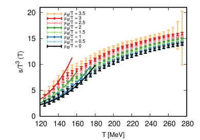
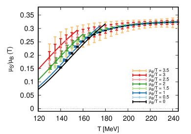
As we already stated, since $\mu^{Q}=0$ and $\chi^{S}_{1}=0$, on the strangeness neutral line we have $c^{B}_{1}=\chi^{B}_{1}$. Therefore, the ansatz in Eq. (16) gives us the baryon number at finite chemical potential directly. In a similar manner, the ratio $\mu_{S}/\mu_{B}$ and the strangeness susceptibility $\chi^{S}_{2}$ are calculated directly from equations (20) and (22) respectively. To obtain the pressure, the entropy density and the energy density, we start with the basic quantity $c^{B}_{1}$. For the pressure, one has to calculate the following integral:

$$\frac{p(T,\hat{\mu}_{B})}{T^{4}}=\frac{p(T,0)}{T^{4}}+\int_{0}^{\hat{\mu}_{B}}c^{B}_{1}(T,\hat{\mu}_{B}^{\prime})\differential\hat{\mu}_{B}^{\prime}\rm{,}$$ (30)

where

$$c^{B}_{1}(T,\hat{\mu}_{B})=c^{B}_{2}(T^{\prime},0)\frac{\overline{c^{B}_{1}}(\hat{\mu}_{B})}{\overline{c^{B}_{2}}(0)}\rm{,}$$ (31)

and the pressure at zero chemical potential is taken from Ref. [58]. The entropy density is defined as

$$s=\frac{\partial p}{\partial T}\Bigg{|}_{\mu_{B},\mu_{S}}\rm{,}$$ (32)

which can be rewritten in terms of dimensionless quantities as:

$$\hat{s} =4\hat{p}+T\frac{\partial\hat{p}}{\partial T}\Bigg{|}_{\mu_{B}}$$ (33)

$$=4\hat{p}+T\frac{\partial\hat{p}}{\partial T}\Bigg{|}_{\hat{\mu}_{B}}-\hat{\mu}_{B}\chi^{B}_{1}\rm{,}$$

where $\hat{s}\equiv\frac{s}{T^{3}}$ and we took into account the difference between derivatives at fixed $\mu_{B}$ versus at fixed $\hat{\mu}_{B}$. By noticing that on the strangeness neutral line

$$\frac{\differential\hat{p}(T,\hat{\mu}_{B},\hat{\mu}_{S}(T,\hat{\mu}_{B}))}{\differential T} =\chi^{S}_{1}\frac{\partial\hat{\mu}_{S}}{\partial T}+\frac{\partial\hat{p}}{\partial T}$$ (34)

$$=\frac{\partial\hat{p}(T,\hat{\mu}_{B},\hat{\mu}_{S}(T,\hat{\mu}_{B}))}{\partial T}\rm{,}$$

we can write the logarithmic temperature derivative of the pressure as:

$$\quad T\left.\frac{\partial\hat{p}(T,\hat{\mu}_{B})}{\partial T}\right|_{\hat{\mu}}=T\frac{\partial\hat{p}(T,0)}{\partial T}$$ (35)

$$\quad\qquad+\frac{1}{2}\int_{0}^{\hat{\mu}_{B}^{2}}T\left.\frac{\differential c^{B}_{2}(T^{\prime},0)}{\differential T^{\prime}}\right|_{T^{\prime}=T\left(1+\lambda_{2}^{BB}y+\lambda_{4}^{BB}y^{2}\right)}\times$$

$$\quad\times\left[1+\lambda_{2}^{BB}y+\lambda_{4}^{BB}y^{2}+T\left(\frac{\differential\lambda_{2}^{BB}}{dT}y+\frac{\differential\lambda_{4}^{BB}}{dT}y^{2}\right)\right]dy$$

where $\frac{\differential c^{B}_{2}(T)}{\differential T}$ is calculated at $\mu_{B}=0$ as discussed previously and presented in Fig. 5.

Given the pressure and the entropy, the dimensionless energy density is given by:

$$\hat{\epsilon}=\hat{s}-\hat{p}+\hat{\mu}_{B}\chi^{B}_{1}\rm{,}$$ (36)

where $\hat{\epsilon}=\frac{\epsilon}{T^{4}}$.

The continuum estimates of the dimensionless baryon number, pressure, entropy density, energy density, $\mu_{S}/\mu_{B}$ ratio and strangeness susceptibility - as computed from the expansion coefficients up to order $\lambda^{ij}_{4}$ - are shown in the various panels of Fig. 8. Notice that even with the inclusion of the $\lambda^{ij}_{4}$ coefficients, the statistical errors of our results stay well under control in the chemical potential range we study. We also compare our results to predictions from the hadron resonance gas model, which at low enough temperatures shows an excellent agreement with our lattice data. As the chemical potential increases, the crossover temperature decreases, and the agreement between out lattice results and the hadron resonance gas gets pushed to lower temperatures, as expected. Note that, similarly to our previous results for the $\mu_{Q}=\mu_{S}=0$ case in Ref. [1], none of the observables display the pathological oscillations of truncated Taylor expansions.

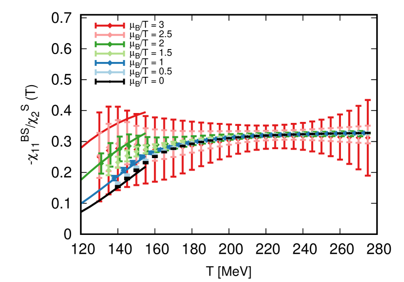
For the extrapolation beyond the strangeness neutral line, the ratio of the baryon-strangeness correlator to the strangeness fluctuations $\chi^{BS}_{11}/\chi^{S}_{2}$ will also be needed. In order to obtain this ratio, we simply note that:

$$-\frac{\chi^{BS}_{11}}{\chi^{S}_{2}} =\frac{\differential\hat{\mu}_{S}}{\differential\hat{\mu}_{B}}$$ (37)

$$=\frac{\differential}{\differential\hat{\mu}_{B}}\left[\hat{\mu}_{B}f_{BS}(T_{BS}^{\prime}(T,\hat{\mu}_{B}))\right]$$

$$=\hat{\mu}_{B}\left[f_{BS}(T_{BS}^{\prime})+\frac{\partial f_{BS}(T_{BS}^{\prime}(T,\hat{\mu}_{B}))}{\partial\hat{\mu}_{B}}\right]\rm{,}$$

where we used the shorthand notation $f_{BS}(T)\equiv\rm{M}(T,0)=-\frac{\chi^{BS}_{11}}{\chi^{S}_{2}}(T,\hat{\mu}_{B}=0)$. Our results for $\chi^{BS}_{11}/\chi^{S}_{2}$ are shown in Fig. 9. In addition to being needed for extrapolation to finite strangeness, this ratio is also of interest for freeze-out phenomenology [78].

V.2 Beyond strangeness neutrality

The quantities calculated so far can also be used to extrapolate the equation of state to small values of the strangeness density, slightly off the $\chi^{S}_{1}=0$ line. Let us denote the value of the dimensionless strange quark chemical potential that solves $\chi^{S}_{1}=0$ at fixed $T$ and $\hat{\mu}_{B}$ as $\hat{\mu}_{S}^{*}$. Still considering a fixed $\hat{\mu}_{B}$ and $T$, but changing $\hat{\mu}_{S}$ slightly from the strangeness neutral choice by a small amount

$$\Delta\hat{\mu}_{S}\equiv\hat{\mu}_{S}-\hat{\mu}_{S}^{\star},$$ (38)

the dimensionless strangeness and baryon densities become:

$$\chi_{1}^{S}(\hat{\mu}_{S}) \approx\chi_{2}^{S}(\hat{\mu}_{S}^{\star})\Delta\hat{\mu}_{S}$$ (39)

$$\chi_{1}^{B}(\hat{\mu}_{S}) \approx\chi_{1}^{B}(\hat{\mu}_{S}^{\star})+\chi_{11}^{BS}(\hat{\mu}_{S}^{\star})\Delta\hat{\mu}_{S}\rm{,}$$ (40)

where we only kept the linear leading order terms in $\Delta\hat{\mu}_{S}$. We will express thermodynamic quantities in terms of the strangeness-to-baryon fraction:

$$R=\frac{\chi_{1}^{S}}{\chi_{1}^{B}}=\frac{\chi_{2}^{S}(\hat{\mu}_{S}^{\star})\Delta\hat{\mu}_{S}}{\chi_{1}^{B}(\hat{\mu}_{S}^{\star})\Delta\hat{\mu}_{S}+\chi_{11}^{BS}(\hat{\mu}_{S}^{\star})}\rm{.}$$ (41)

Inverting this equation we get:

$$\Delta\hat{\mu}_{S}=\frac{R\hat{\chi}^{B}_{1}(\hat{\mu}_{S}^{\star})}{\chi_{2}^{S}(\hat{\mu}_{S}^{\star})-R\chi_{11}^{BS}(\hat{\mu}_{S}^{\star})}\rm{.}$$ (42)

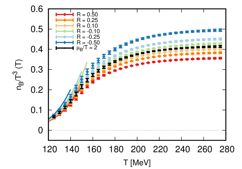
This quantity is shown for $\hat{\mu}_{B}=2$ as a function of temperature for various value of $R$ in Fig. 10. Substituting Eq. (42) into Eq. (40) we obtain - to leading order in $R$:

$$\frac{\chi^{B}_{1}(T,\hat{\mu}_{B},R)}{\chi^{B}_{1}(T,\hat{\mu}_{B},R=0)}\approx 1+R\frac{\chi^{BS}_{11}(T,\hat{\mu}_{B},R=0)}{\chi^{S}_{2}(T,\hat{\mu}_{B},R=0)}\rm{,}$$ (43)

where all quantities on the right hand side are along the strangeness neutral line. We show the results of a leading order extrapolation of the dimensionless baryon density as a function of $T$ at $\hat{\mu}_{B}=2$ for several values of $R$ in Fig. 11.

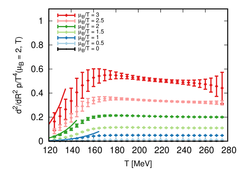
At the strangeness neutral line the $\mathcal{O}(R)$ correction of the pressure vanishes. The leading order correction gives:

$$\hat{p}(T,\hat{\mu}_{B},R)\approx\hat{p}(T,\hat{\mu}_{B},R)+\frac{1}{2}\frac{\differential^{2}\hat{p}}{\differential R^{2}}\left(T,\hat{\mu}_{B}\right)R^{2}\rm{,}$$ (44)

where

$$\frac{\differential^{2}\hat{p}}{\differential R^{2}}\left(T,\hat{\mu}_{B}\right)=\frac{\left(\chi^{B}_{1}\left(T,\hat{\mu}_{B}\right)\right)^{2}}{\chi^{S}_{2}\left(T,\hat{\mu}_{B}\right)}\rm{.}$$ (45)

This leading order coefficient is show in Fig. 12 for several values of $\hat{\mu}_{B}$.

Figure 9: The ratio $\chi^{BS}_{11}/\chi^{S}_{2}$ as a function of the temperature for several values of $\hat{\mu}_{B}$.

Figure 10: Shift of the strangeness chemical potential as a function of the temperature at $\hat{\mu}_{B}=2$, at various values of the strangeness-to-baryon ratio $R=\chi^{S}_{1}/\chi^{B}_{1}$. The solid lines show the exact solution of $0.4\chi^{B}_{1}=\chi^{S}_{1}$ in the hadron resonance (HRG) model, while the dashed lines show the evaluation of the approximation of Eq. (42) in the HRG model.

Figure 11: The dimensionless baryon density as a function of the temperature at $\hat{\mu}_{B}=2$, for various values of the strangeness-to-baryon $R=\chi^{S}_{1}/\chi^{B}_{1}$.

Figure 12: The leading order Taylor coefficient of the pressure in the strangeness-to-baryon ratio $R$ on the strangeness neutral line as a function of the temperature for several fixed values of $\hat{\mu}_{B}$.

VI Summary and discussion

In this work, we generalized the extrapolation procedure we introduced in Ref. [1] for the equation of state to the case of strangeness neutrality. Using zero and imaginary chemical potential simulations we determined the first two coefficients in the scheme $\lambda^{ij}_{2}$ and $\lambda^{ij}_{4}$ for the baryon density, the strangeness chemical potential and the strangeness fluctuations. Using these coefficients, we extrapolated the equation of state up to a baryochemical potential-to-temperature ratio of $\hat{\mu}_{B}=3.5$, considerably improving the range covered by first principle lattice calculations. Just like for the case of $\mu_{S}=\mu_{Q}=0$ in Ref. [1], also for the strangeness neutral case we observed that our extrapolation scheme is free of the unphysical oscillations that plague the fixed order Taylor expansions at higher chemical potentials.

We also introduced a Stefan-Boltzmann correction to improve the rate of convergence of our scheme at high temperatures. Due to this correction, the coefficient $\lambda^{BB}_{2}$ goes to zero at high temperatures.

We moved beyond strangeness neutrality by calculating the baryon-strangeness correlator to strangeness susceptibility ratio $\chi^{BS}_{11}/\chi^{S}_{2}$ at finite real $\hat{\mu}_{B}$ on the strangeness neutral line. This allows one to perform a leading order extrapolation of the baryon number in the ratio $R=\chi^{S}_{1}/\chi^{B}_{1}$.

Apart from increasing precision through higher statistics, this work can be extended in the future to to take the small isospin imbalance $\chi^{Q}_{1}=0.4\chi^{B}_{1}$ of lead and gold nuclei into account beyond leading order. With significantly more data taking, a full scan of the $\mu_{B}-\mu_{S}$ plane is possible, thus determining the equation of state for higher values of the strangeness-to-baryon ratio. It will be valuable to see whether the calculation of even higher order coefficients (e.g. $\kappa^{ij}_{6}$) will alter the presented picture or introduce significant improvements in the range explored by the RHIC Beam Energy Scan program.

We also mention that, while for the ordinary Taylor expansion of the pressure estimates of the radius of convergence exist both on coarse lattices [27, 28, 79, 71] and from phenomenological arguments  [80, 81], the ultimate convergence properties of our scheme are completely unknown at the moment. As our ansatz is not a Taylor series for the pressure, its domain of convergence is not necessarily a circle in the complex plane. Furthermore, the scheme is generalizable also for non-polynomial approximations of $T^{\prime}$, such as rational functions. The domain of convergence of our scheme is an interesting theoretical question. It, however, has no practical consequence at the moment, as the $\lambda^{ij}_{4}$ are already consistent with zero, leading to fast apparent convergence at low orders.

Appendix: $\lambda^{ij}_{2}$ coefficients from Taylor coefficients

For reference, we list here the relationships between our $\lambda_{2}$ coefficients and ordinary Taylor coefficients. For the expansion coefficient of the baryon density, we get:

$$\lambda_{2}^{\rm BB}=\frac{1}{6Tf^{\prime}(T)}\left(c_{4}^{B}(0,T)-\frac{\overline{c_{4}^{B}}(0)}{\overline{c_{2}^{B}}(0)}f(T)\right)$$

where $f(T)=\frac{\differential^{2}logZ}{\differential\mu_{B}^{2}}(\mu_{B}=0,T)$. For the expansion coefficient of the strangeness chemical potential we get

$$\lambda_{2}^{\rm BS}=\frac{1}{Tf^{\prime}(T)}s_{3}(T)=\frac{1}{6Tf^{\prime}(T)}\frac{\differential^{3}\hat{\mu}_{S}}{\differential\hat{\mu}_{B}^{3}}(T)$$

where $\frac{\hat{\mu}_{S}}{\hat{\mu}_{B}}(\hat{\mu}_{B},T)=s_{1}(T)+s_{3}(T)\hat{\mu}_{B}^{2}+s_{5}(T)\hat{\mu}_{B}^{4}+\dots$ and $f(T)=\lim_{\hat{\mu}_{B}\rightarrow 0}\frac{\hat{\mu}_{S}}{\hat{\mu}_{B}}(\mu_{B},T)=-\frac{\chi_{11}^{BS}}{\chi_{2}^{S}}(0,T)$. For the expansion coefficient of the strangeness susceptibility we get

$$\lambda_{2}^{\rm SS}=\frac{1}{2\,Tf^{\prime}(T)}S_{2,\rm sym}^{\rm NLO}(0,T)$$

where $f(T)=\chi_{2}^{S}(\mu_{B}=0,T)$.

In principle, the $\lambda_{4}$ coefficients can also be expressed using the Taylor coefficients at $\mu\equiv 0$. For this one needs The Taylor coefficients up to sixth order and the second temperature derivative of the second order coefficients. For the quantities discussed in this paper we give:

$$\lambda_{4}^{\rm BB}(T) =\frac{1}{360T}\frac{1}{{\overline{c}_{2}^{B}(0)}^{2}{f^{\prime}(T)}^{3}}\cdot$$

$$\left[3\,{\overline{c}_{2}^{B}(0)}^{2}c_{6}^{B}(0,T){f^{\prime}(T)}^{2}\right.$$ (46)

$$\left.-10\,\overline{c}_{4}^{B}(0)\,{f^{\prime}(T)}^{2}\,\left(\overline{c}_{2}^{B}(0)c_{4}^{B}(0,T)-\overline{c}_{4}^{B}(0)f(T)\right)\right.$$

$$\left.-5\,f^{\prime\prime}(T)\left(\overline{c}_{2}^{B}(0)c_{4}^{B}(0,T)-\overline{c}_{4}^{B}(0)f(T)\right)^{2}\right]\,\,$$

$$\lambda_{4}^{\rm BS}(T) =\frac{s_{5}(T)}{Tf^{\prime}(T)}-\frac{s_{3}(T)^{2}f^{\prime\prime}(T)}{2Tf^{\prime}(T)^{3}}$$ (47)

$$=\frac{1}{120Tf^{\prime}(T)}\frac{\differential^{5}\hat{\mu}_{S}}{\differential\hat{\mu}_{B}^{5}}(T)-\frac{f^{\prime\prime}(T)}{72Tf^{\prime}(T)^{3}}\left(\frac{\differential^{3}\hat{\mu}_{S}}{\differential\hat{\mu}_{B}^{3}}(T)\right)^{2}\,\,$$

$$\lambda_{4}^{\rm SS}(T) =\frac{1}{24Tf^{\prime}(T)^{3}}\Bigl{(}S_{2,\rm sym}^{\rm NNLO}(0,T)f^{\prime}(T)^{2}$$

$$-3f^{\prime\prime}(T)S_{2,\rm sym}^{\rm NLO}(0,T)^{2}\Bigr{)}\,\,$$ (48)

with

$$S_{2,\rm sym}^{\rm NLO}(0,T) =\chi_{22}^{BS}(0,T)$$

$$+2s_{1}(T)\chi_{13}^{BS}(0,T)+s_{1}(T)^{2}\chi_{4}^{S}(0,T)$$ (49)

$$S_{2,\rm sym}^{\rm NNLO}(0,T) =\chi_{42}^{BS}(0,T)+4s_{1}(T)\chi_{33}^{BS}(0,T)$$

$$+6s_{1}(T)^{2}\chi_{24}^{BS}(0,T)+4s_{1}(T)^{3}\chi_{15}^{BS}(0,T)$$

$$+s_{1}(T)^{4}\chi_{6}^{S}(0,T)+24s_{3}(T)\chi_{13}^{BS}(0,T)$$

$$+24\chi^{S}_{4}(0,T)s_{1}(T)s_{3}(T)$$ (50)

where we used the expansion coefficients of $\mu_{S}(\mu_{B})$:

$$s_{1} = -\frac{\chi_{11}^{BS}}{\chi_{2}^{S}}$$ (51)

$$s_{3} = -\frac{1}{6\chi_{2}^{S}}\left[\chi_{4}^{S}s_{1}^{3}+3\chi_{13}^{BS}s_{1}^{2}+3\chi_{22}^{BS}s_{1}+\chi_{31}^{BS}\right]$$ (52)

$$s_{5} = -\frac{1}{120\chi_{2}^{S}}\bigl{[}+\chi_{6}^{S}s_{1}^{5}+5\chi_{15}^{BS}s_{1}^{4}+10\chi_{24}^{BS}s_{1}^{3}$$ (53)

$$+60\chi_{4}^{S}s_{1}^{2}s_{3}+120\chi_{13}^{BS}s_{1}s_{3}+60\chi_{22}^{BS}s_{3}$$

$$+10\chi_{33}^{BS}s_{1}^{2}+5\chi_{42}^{BS}s_{1}+\chi_{51}^{BS}\bigr{]}$$

References

- [1] S. Borsányi, Z. Fodor, J. N. Guenther, R. Kara, S. D. Katz, P. Parotto, A. Pásztor, C. Ratti, and K. K. Szabó. Lattice QCD equation of state at finite chemical potential from an alternative expansion scheme. Phys. Rev. Lett., 126(23):232001, 2021.
- [2] Y. Aoki, G. Endrodi, Z. Fodor, S. D. Katz, and K. K. Szabo. The Order of the quantum chromodynamics transition predicted by the standard model of particle physics. Nature, 443:675–678, 2006.
- [3] Kenji Fukushima and Chihiro Sasaki. The phase diagram of nuclear and quark matter at high baryon density. Prog. Part. Nucl. Phys., 72:99–154, 2013.
- [4] Peter Kovács, Zsolt Szép, and György Wolf. Existence of the critical endpoint in the vector meson extended linear sigma model. Phys. Rev. D, 93(11):114014, 2016.
- [5] Renato Critelli, Jorge Noronha, Jacquelyn Noronha-Hostler, Israel Portillo, Claudia Ratti, and Romulo Rougemont. Critical point in the phase diagram of primordial quark-gluon matter from black hole physics. Phys. Rev. D, 96(9):096026, 2017.
- [6] Philipp Isserstedt, Michael Buballa, Christian S. Fischer, and Pascal J. Gunkel. Baryon number fluctuations in the QCD phase diagram from Dyson-Schwinger equations. Phys. Rev. D, 100(7):074011, 2019.
- [7] Julian Bernhardt, Christian S. Fischer, Philipp Isserstedt, and Bernd-Jochen Schaefer. Critical endpoint of QCD in a finite volume. Phys. Rev. D, 104(7):074035, 2021.
- [8] Fei Gao and Jan M. Pawlowski. Chiral phase structure and critical end point in QCD. Phys. Lett. B, 820:136584, 2021.
- [9] Gert Aarts. Introductory lectures on lattice QCD at nonzero baryon number. J. Phys. Conf. Ser., 706(2):022004, 2016.
- [10] Keitaro Nagata. Finite-density lattice QCD and sign problem: current status and open problems. 8 2021.
- [11] A. Hasenfratz and D. Toussaint. Canonical ensembles and nonzero density quantum chromodynamics. Nucl. Phys. B, 371:539–549, 1992.
- [12] Z. Fodor and S. D. Katz. A New method to study lattice QCD at finite temperature and chemical potential. Phys. Lett. B, 534:87–92, 2002.
- [13] Z. Fodor and S. D. Katz. Lattice determination of the critical point of QCD at finite T and mu. JHEP, 03:014, 2002.
- [14] Z. Fodor, S. D. Katz, and K. K. Szabo. The QCD equation of state at nonzero densities: Lattice result. Phys. Lett. B, 568:73–77, 2003.
- [15] Z. Fodor and S. D. Katz. Critical point of QCD at finite T and mu, lattice results for physical quark masses. JHEP, 04:050, 2004.
- [16] Matteo Giordano, Kornel Kapas, Sandor D. Katz, Daniel Nogradi, and Attila Pasztor. Effect of stout smearing on the phase diagram from multiparameter reweighting in lattice QCD. Phys. Rev. D, 102(3):034503, 2020.
- [17] Matteo Giordano, Kornel Kapas, Sandor D. Katz, Daniel Nogradi, and Attila Pasztor. New approach to lattice QCD at finite density; results for the critical end point on coarse lattices. JHEP, 05:088, 2020.
- [18] C. R. Allton, S. Ejiri, S. J. Hands, O. Kaczmarek, F. Karsch, E. Laermann, C. Schmidt, and L. Scorzato. The QCD thermal phase transition in the presence of a small chemical potential. Phys. Rev., D66:074507, 2002.
- [19] C. R. Allton, M. Doring, S. Ejiri, S. J. Hands, O. Kaczmarek, F. Karsch, E. Laermann, and K. Redlich. Thermodynamics of two flavor QCD to sixth order in quark chemical potential. Phys. Rev., D71:054508, 2005.
- [20] R. V. Gavai and Sourendu Gupta. QCD at finite chemical potential with six time slices. Phys. Rev., D78:114503, 2008.
- [21] Szabolcs Borsányi, Zoltán Fodor, Sándor D. Katz, Stefan Krieg, Claudia Ratti, and Kálmán Szabó. Fluctuations of conserved charges at finite temperature from lattice QCD. JHEP, 01:138, 2012.
- [22] Sz. Borsányi, G. Endrődi, Z. Fodor, S.D. Katz, S. Krieg, et al. QCD equation of state at nonzero chemical potential: continuum results with physical quark masses at order . JHEP, 1208:053, 2012.
- [23] R. Bellwied, S. Borsányi, Z. Fodor, S. D. Katz, A. Pásztor, C. Ratti, and K. K. Szabó. Fluctuations and correlations in high temperature QCD. Phys. Rev., D92(11):114505, 2015.
- [24] H. T. Ding, Swagato Mukherjee, H. Ohno, P. Petreczky, and H. P. Schadler. Diagonal and off-diagonal quark number susceptibilities at high temperatures. Phys. Rev., D92(7):074043, 2015.
- [25] A. Bazavov et al. The QCD Equation of State to from Lattice QCD. Phys. Rev. D, 95(5):054504, 2017.
- [26] Zoltán Fodor, Matteo Giordano, Jana N. Günther, Kornél Kapás, Sándor D. Katz, Attila Pásztor, Israel Portillo, Claudia Ratti, Dénes Sexty, and Kálman K. Szabó. Trying to constrain the location of the QCD critical endpoint with lattice simulations. Nucl. Phys. A, 982:843–846, 2019.
- [27] Matteo Giordano and Attila Pásztor. Reliable estimation of the radius of convergence in finite density QCD. Phys. Rev. D, 99(11):114510, 2019.
- [28] Matteo Giordano, Kornel Kapas, Sandor D. Katz, Daniel Nogradi, and Attila Pasztor. Radius of convergence in lattice QCD at finite with rooted staggered fermions. Phys. Rev. D, 101(7):074511, 2020.
- [29] A. Bazavov et al. Skewness, kurtosis, and the fifth and sixth order cumulants of net baryon-number distributions from lattice QCD confront high-statistics STAR data. Phys. Rev. D, 101(7):074502, 2020.
- [30] Philippe de Forcrand and Owe Philipsen. The QCD phase diagram for small densities from imaginary chemical potential. Nucl. Phys., B642:290–306, 2002.
- [31] Massimo D’Elia and Maria Paola Lombardo. Finite density QCD via imaginary chemical potential. Phys. Rev., D67:014505, 2003.
- [32] Massimo D’Elia and Francesco Sanfilippo. Thermodynamics of two flavor QCD from imaginary chemical potentials. Phys. Rev., D80:014502, 2009.
- [33] Paolo Cea, Leonardo Cosmai, and Alessandro Papa. Critical line of 2+1 flavor QCD. Phys. Rev., D89(7):074512, 2014.
- [34] Claudio Bonati, Philippe de Forcrand, Massimo D’Elia, Owe Philipsen, and Francesco Sanfilippo. Chiral phase transition in two-flavor QCD from an imaginary chemical potential. Phys. Rev., D90(7):074030, 2014.
- [35] Paolo Cea, Leonardo Cosmai, and Alessandro Papa. Critical line of 2+1 flavor QCD: Toward the continuum limit. Phys. Rev., D93(1):014507, 2016.
- [36] Claudio Bonati, Massimo D’Elia, Marco Mariti, Michele Mesiti, Francesco Negro, and Francesco Sanfilippo. Curvature of the chiral pseudocritical line in QCD: Continuum extrapolated results. Phys. Rev. D, 92(5):054503, 2015.
- [37] R. Bellwied, S. Borsányi, Z. Fodor, J. Günther, S. D. Katz, C. Ratti, and K. K. Szabó. The QCD phase diagram from analytic continuation. Phys. Lett., B751:559–564, 2015.
- [38] Massimo D’Elia, Giuseppe Gagliardi, and Francesco Sanfilippo. Higher order quark number fluctuations via imaginary chemical potentials in QCD. Phys. Rev. D, 95(9):094503, 2017.
- [39] J. N. Günther, R. Bellwied, S. Borsányi, Z. Fodor, S. D. Katz, A. Pásztor, C. Ratti, and K. K. Szabó. The QCD equation of state at finite density from analytical continuation. Nucl. Phys., A967:720–723, 2017.
- [40] Paolo Alba et al. Constraining the hadronic spectrum through QCD thermodynamics on the lattice. Phys. Rev. D, 96(3):034517, 2017.
- [41] Volodymyr Vovchenko, Attila Pasztor, Zoltan Fodor, Sandor D. Katz, and Horst Stoecker. Repulsive baryonic interactions and lattice QCD observables at imaginary chemical potential. Phys. Lett. B, 775:71–78, 2017.
- [42] Claudio Bonati, Massimo D’Elia, Francesco Negro, Francesco Sanfilippo, and Kevin Zambello. Curvature of the pseudocritical line in QCD: Taylor expansion matches analytic continuation. Phys. Rev., D98(5):054510, 2018.
- [43] Szabolcs Borsányi, Zoltán Fodor, Jana N. Günther, Sándor K. Katz, Kálmán K. Szabó, Attila Pásztor, Israel Portillo, and Claudia Ratti. Higher order fluctuations and correlations of conserved charges from lattice QCD. JHEP, 10:205, 2018.
- [44] Szabolcs Borsanyi, Zoltan Fodor, Jana N. Guenther, Ruben Kara, Sandor D. Katz, Paolo Parotto, Attila Pasztor, Claudia Ratti, and Kalman K. Szabo. QCD Crossover at Finite Chemical Potential from Lattice Simulations. Phys. Rev. Lett., 125(5):052001, 2020.
- [45] Attila Pásztor, Zsolt Szép, and Gergely Markó. Apparent convergence of Pad\’e approximants for the crossover line in finite density QCD. 10 2020.
- [46] Zoltan Fodor, Sandor D. Katz, and Christian Schmidt. The Density of states method at non-zero chemical potential. JHEP, 03:121, 2007.
- [47] Szabolcs Borsanyi, Zoltan Fodor, Matteo Giordano, Sandor D. Katz, Daniel Nogradi, Attila Pasztor, and Chik Him Wong. Lattice simulations of the QCD chiral transition at real baryon density. 8 2021.
- [48] Gert Aarts, Erhard Seiler, and Ion-Olimpiu Stamatescu. The Complex Langevin method: When can it be trusted? Phys. Rev. D, 81:054508, 2010.
- [49] Dénes Sexty. Simulating full QCD at nonzero density using the complex Langevin equation. Phys. Lett. B, 729:108–111, 2014.
- [50] M. Scherzer, E. Seiler, D. Sexty, and I. O. Stamatescu. Controlling Complex Langevin simulations of lattice models by boundary term analysis. Phys. Rev. D, 101(1):014501, 2020.
- [51] Marco Cristoforetti, Francesco Di Renzo, and Luigi Scorzato. New approach to the sign problem in quantum field theories: High density QCD on a Lefschetz thimble. Phys. Rev. D, 86:074506, 2012.
- [52] Andrei Alexandru, Gökçe Basar, and Paulo Bedaque. Monte Carlo algorithm for simulating fermions on Lefschetz thimbles. Phys. Rev. D, 93(1):014504, 2016.
- [53] Masafumi Fukuma, Nobuyuki Matsumoto, and Naoya Umeda. Implementation of the HMC algorithm on the tempered Lefschetz thimble method. 12 2019.
- [54] Paul Romatschke. New Developments in Relativistic Viscous Hydrodynamics. Int. J. Mod. Phys. E, 19:1–53, 2010.
- [55] Ulrich W. Heinz. Towards the Little Bang Standard Model. J. Phys. Conf. Ser., 455:012044, 2013.
- [56] Scott Pratt, Evan Sangaline, Paul Sorensen, and Hui Wang. Constraining the Eq. of State of Super-Hadronic Matter from Heavy-Ion Collisions. Phys. Rev. Lett., 114:202301, 2015.
- [57] Szabolcs Borsanyi, Gergely Endrodi, Zoltan Fodor, Antal Jakovac, Sandor D. Katz, Stefan Krieg, Claudia Ratti, and Kalman K. Szabo. The QCD equation of state with dynamical quarks. JHEP, 11:077, 2010.
- [58] Szabolcs Borsanyi, Zoltan Fodor, Christian Hoelbling, Sandor D. Katz, Stefan Krieg, and Kalman K. Szabo. Full result for the QCD equation of state with 2+1 flavors. Phys. Lett. B, 730:99–104, 2014.
- [59] A. Bazavov et al. Equation of state in ( 2+1 )-flavor QCD. Phys. Rev. D, 90:094503, 2014.
- [60] Sz. Borsanyi et al. Calculation of the axion mass based on high-temperature lattice quantum chromodynamics. Nature, 539(7627):69–71, 2016.
- [61] K. Kajantie, M. Laine, K. Rummukainen, and Y. Schroder. The Pressure of hot QCD up to g6 ln(1/g). Phys. Rev. D, 67:105008, 2003.
- [62] Jens O. Andersen, Lars E. Leganger, Michael Strickland, and Nan Su. NNLO hard-thermal-loop thermodynamics for QCD. Phys. Lett. B, 696:468–472, 2011.
- [63] Jens O. Andersen, Lars E. Leganger, Michael Strickland, and Nan Su. Three-loop HTL QCD thermodynamics. JHEP, 08:053, 2011.
- [64] Sylvain Mogliacci, Jens O. Andersen, Michael Strickland, Nan Su, and Aleksi Vuorinen. Equation of State of hot and dense QCD: Resummed perturbation theory confronts lattice data. JHEP, 12:055, 2013.
- [65] Najmul Haque, Aritra Bandyopadhyay, Jens O. Andersen, Munshi G. Mustafa, Michael Strickland, and Nan Su. Three-loop HTLpt thermodynamics at finite temperature and chemical potential. JHEP, 05:027, 2014.
- [66] Najmul Haque and Michael Strickland. Next-to-next-to leading-order hard-thermal-loop perturbation-theory predictions for the curvature of the QCD phase transition line. Phys. Rev. C, 103(3):031901, 2021.
- [67] Claudia Ratti, Simon Roessner, and Wolfram Weise. Quark number susceptibilities: Lattice QCD versus PNJL model. Phys. Lett. B, 649:57–60, 2007.
- [68] Paolo Parotto, Marcus Bluhm, Debora Mroczek, Marlene Nahrgang, Jacquelyn Noronha-Hostler, Krishna Rajagopal, Claudia Ratti, Thomas Schäfer, and Mikhail Stephanov. QCD equation of state matched to lattice data and exhibiting a critical point singularity. Phys. Rev. C, 101(3):034901, 2020.
- [69] J. M. Karthein, D. Mroczek, A. R. Nava Acuna, J. Noronha-Hostler, P. Parotto, D. R. P. Price, and C. Ratti. Strangeness-neutral equation of state for QCD with a critical point. Eur. Phys. J. Plus, 136(6):621, 2021.
- [70] Saumen Datta, Rajiv V. Gavai, and Sourendu Gupta. Quark number susceptibilities and equation of state at finite chemical potential in staggered QCD with Nt=8. Phys. Rev. D, 95(5):054512, 2017.
- [71] P. Dimopoulos, L. Dini, F. Di Renzo, J. Goswami, G. Nicotra, C. Schmidt, S. Singh, K. Zambello, and F. Ziesché. A contribution to understanding the phase structure of strong interaction matter: Lee-Yang edge singularities from lattice QCD. 10 2021.
- [72] H. T. Ding et al. Chiral Phase Transition Temperature in ( 2+1 )-Flavor QCD. Phys. Rev. Lett., 123(6):062002, 2019.
- [73] Andrey Yu. Kotov, Maria Paola Lombardo, and Anton Trunin. QCD transition at the physical point, and its scaling window from twisted mass Wilson fermions. Phys. Lett. B, 823:136749, 2021.
- [74] Throughout this work, we always use the continuum Stefan-Boltzmann limits.
- [75] Colin Morningstar and Mike J. Peardon. Analytic smearing of SU(3) link variables in lattice QCD. Phys. Rev. D, 69:054501, 2004.
- [76] M. Tanabashi et al. Review of Particle Physics. Phys. Rev. D, 98(3):030001, 2018.
- [77] Szabolcs Borsanyi et al. High-precision scale setting in lattice QCD. JHEP, 09:010, 2012.
- [78] Rene Bellwied, Szabolcs Borsanyi, Zoltan Fodor, Jana N. Guenther, Jacquelyn Noronha-Hostler, Paolo Parotto, Attila Pasztor, Claudia Ratti, and Jamie M. Stafford. Off-diagonal correlators of conserved charges from lattice QCD and how to relate them to experiment. Phys. Rev. D, 101(3):034506, 2020.
- [79] Sourav Mondal, Swagato Mukherjee, and Prasad Hegde. Lattice QCD Equation of State for Nonvanishing Chemical Potential by Resumming Taylor Expansions. Phys. Rev. Lett., 128(2):022001, 2022.
- [80] M. A. Stephanov. QCD critical point and complex chemical potential singularities. Phys. Rev. D, 73:094508, 2006.
- [81] Swagato Mukherjee and Vladimir Skokov. Universality driven analytic structure of the QCD crossover: radius of convergence in the baryon chemical potential. Phys. Rev. D, 103(7):L071501, 2021.