A Directional Equispaced interpolation-based
Fast Multipole Method for oscillatory kernels

Abstract

Fast Multipole Methods (FMMs) based on the oscillatory Helmholtz kernel can reduce the cost of solving N-body problems arising from Boundary Integral Equations (BIEs) in acoustic or electromagnetics. However, their cost strongly increases in the high-frequency regime. This paper introduces a new directional FMM for oscillatory kernels (defmm - directional equispaced interpolation-based fmm), whose precomputation and application are FFT-accelerated due to polynomial interpolations on equispaced grids. We demonstrate the consistency of our FFT approach, and show how symmetries can be exploited in the Fourier domain. We also describe the algorithmic design of defmm, well-suited for the BIE non-uniform particle distributions, and present performance optimizations on one CPU core. Finally, we exhibit important performance gains on all test cases for defmm over a state-of-the-art FMM library for oscillatory kernels.

1 Introduction

Considering two point clouds $X,Y\subset\mathbb{R}^{d}$ with cardinal $N\in\mathbb{N}^{*}$, $d\in\mathbb{N}^{*}$ and $q\in\mathbb{C}[Y]$ (named charges), where $\mathbb{C}[Y]$ denotes the set of application from $Y$ to $\mathbb{C}$, we are interested in the fast computation of $p\in\mathbb{C}[X]$ (referred to as potentials) such that

$$p(\mathbf{x}):=\sum_{\mathbf{y}\in Y}G(\mathbf{x},\mathbf{y})q(\mathbf{y}),\hskip 14.22636pt\forall\hskip 1.42271pt\mathbf{x}\in X,$$ (1)

where $G\hskip 1.42271pt:\hskip 1.42271pt\mathbb{R}^{d}\times\mathbb{R}^{d}\rightarrow\mathbb{C}$. Such an N-body problem appears in the numerical solving of Boundary Integral Equations (BIEs). We are especially concerned by the oscillatory Helmholtz kernel involved in BIEs applied to acoustic or electromagnetics

$$G(\mathbf{x},\mathbf{y}):=\frac{e^{i\kappa|\mathbf{x}-\mathbf{y}|}}{4\pi|\mathbf{x}-\mathbf{y}|},$$

where $\kappa\in\mathbb{R}^{+}$ is named the wavenumber, $i$ denotes the complex number and $|\cdot|$ refers to the Euclidian norm. Computing $p$ using hierarchical methods can achieve an $\mathcal{O}(N\hskip 0.56917pt\log\hskip 0.56917ptN)$ complexity on large surface particle distributions (i.e. point clouds), that are the distributions generated when discretizing BIEs. However, the cost of the hierarchical methods can still be a bottleneck in the high-frequency regime, i.e. when $\kappa D\gg 1$, $D$ denoting the side length of the smallest box encompassing $X$ and $Y$.

1.1 Related work

The direct evaluation of the N-body problem (1) has a complexity $\mathcal{O}(N^{2})$. This complexity can be reduced using a hierarchical method, such as the Fast Multipole Method (FMM) [21, 11]. Thanks to a hierarchical decomposition, such as a $2^{d}$-tree representation of the (cubical) computational domain $B$, and to a multipole acceptance criterion, the computation of (1) is indeed divided into two parts: a near field one which is computed directly and a far field one which is approximated through multipole and local expansions. Nodes of such a $2^{d}$-tree are named cells and correspond to cubical subdomains of $B$ whose radii depend on the tree level (see Figure 1).

Figure 1: $2^{d}$-tree ($d=2$) representation of $B$ with particles colored in blue.

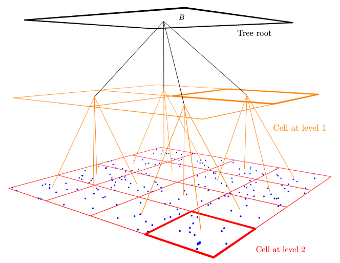
There mainly exist two approaches for FMMs dealing with the high-frequency Helmholtz kernel. First, the kernel-explicit methods consist in an explicit diagonalization of large far-field matrix blocks using analytic kernel expansions [11, 9], considering that the $N$-body problem in equation 1 is interpreted as a matrix-vector product. These methods perform differently depending on the particle distribution, with complexities up to $\mathcal{O}(N^{3/2})$ (see [9]). Second, the kernel-independent methods (see for instance [16, 32]) allow to use the same formalism, hence the same implementation, for a given class of kernels. Based on a specific definition of the well-separateness (i.e. the subsets of $B\times B$ on which the far-field approximations can be applied), the directional kernel-independent approaches exploit the low-rank property of particular blocks of a modified kernel [15, 25, 6]. As opposed to the kernel-explicit methods, the kernel-independent directional approaches allow to derive fast algorithms with complexity $\mathcal{O}(N\hskip 1.42271pt\log\hskip 0.56917ptN)$ regardless of the particle distribution (see [25]).

The directional FMM algorithms described in the literature exploit low-rank approximations to compress matrices representing the far-field contributions [15, 25, 24]. However, some highly efficient kernel-independent methods for low-frequency and translation-invariant kernels use Fast Fourier Transforms (FFTs) to efficiently process these matrices in diagonal form [30]. These FFT-based methods exploit equispaced grids (i.e. cartesian grids or tensorization of the same uniform sampling $d$ times). In FMM formulations based on polynomial interpolation, the use of FFT techniques was shown to be more efficient than low-rank approximations in the low-frequency regime [5], especially for high approximation orders. To our knowledge, directional FFT-based FMMs for the high-frequency regime have not been investigated in the past. Moreover, in such polynomial interpolation-based FMMs, the matrices associated to some FMM operators have to be precomputed, but their number drastically increases in the high-frequency regime (see [24]), which strongly increases the precomputation cost. FFT techniques can also help to reduce such precomputation cost.

In this paper, we aim at efficiently solving the N-body problem (1) with oscillatory kernels in both low- and high-frequency regimes. We thus present the first directional (hence $\mathcal{O}\left(N\hskip 1.42271ptlog\hskip 1.42271ptN\right)$) interpolation-based FMM taking advantage of polynomial interpolation on equispaced grids to allow fast FFT-based evaluations and precomputations of the far-field matrices. A consistency proof for the polynomial Lagrange interpolation on such grids and on well-separated sets when dealing with asymptotically smooth kernels is provided. This gives a rigorous explanation of the practical convergence of our approximation process despite the well-known stability issue of such polynomial interpolation. We also show how to extend the use of some symmetries in the Fourier domain in order to minimize the number of precomputed matrices. FMMs can rely on different $2^{d}$-tree traversals: we adapt here a specific one (namely the dual tree traversal) to directional FMMs and show its relevance, along with a suitable $2^{d}$-tree data structure, for the non-uniform particle distributions typical of BIE problems. We provide a new, publicly available, C++ library implementing our FMM, named as defmm (directional equispaced interpolation-based fmm) and highly optimized on one CPU core. We detail the vectorization process of our near-field direct computation using high-level programming, and we show how to efficiently process the numerous and small FFTs required in our method. We also improve the performance of the BLAS-based operators in the multipole and local expansion translations. Finally, we detail a comparison with a state-of-the-art directional polynomial interpolation-based FMM library (namely dfmm [25, 24]), exhibiting important performance gains for defmm in all the test cases.

The paper is organized as follows. In section 2, we first recall the mathematical bases of the FMMs involved in this paper. We then provide in section 3 a consistency proof of our interpolation process on equispaced grids. We detail in section 4 the defmm algorithmic design and we show how to extend and exploit the tree symmetries in the Fourier domain. In section 5, we present various HPC optimizations on one CPU core for defmm, and finally in section 6 we provide numerical results, including a detailed performance comparison.

2 Presentation of Fast Multipole Methods

We focus in this article on the FMM formulation using polynomial interpolation and its variants [16, 30, 25], which are here briefly recalled.

2.1 Directional FMMs

Suppose that the kernel $G$ can be factorized into

$$G(\mathbf{x},\mathbf{y})=e^{i\kappa|\mathbf{x}-\mathbf{y}|}K(\mathbf{x},\mathbf{y}),$$ (2)

where $K$ is an asymptotically smooth non-oscillatory kernel. Directional approaches rely on the directional parabolic separation condition (DPSC) [15], imposing conditions on well-separated subsets of $B\times B$ (i.e. pairs of cells in practice) such that the term $G_{u}$ in the expression

$$G(\mathbf{x},\mathbf{y})=e^{i\kappa\langle\mathbf{x},u\rangle}\underbrace{\left(e^{i\kappa\langle\mathbf{x}-\mathbf{y},\frac{\mathbf{x}-\mathbf{y}}{|\mathbf{x}-\mathbf{y}|}-u\rangle}K(\mathbf{x},\mathbf{y})\right)}_{=:G_{u}(\mathbf{x},\mathbf{y})}e^{-i\kappa\langle\mathbf{y},u\rangle}$$ (3)

does not oscillate, where $u\in\mathbb{S}^{2}$ (referred to as a direction) is a well-chosen approximation of $(\mathbf{x}-\mathbf{y})/|\mathbf{x}-\mathbf{y}|$ on the unit sphere. Since the only term in equation (3) depending on both $\mathbf{x}$ and $\mathbf{y}$ is $G_{u}$, fast summation methods can be derived. The DPSC is verified when $\mathbf{x}\in t$, $\mathbf{y}\in s$, where $t,s$ are two cells such that

$$\kappa\hskip 0.56917ptw^{2}\leq\eta\hskip 1.13791ptdist(t,s)\text{ and }t\subset C(s),$$ (4)

with $dist(t,s):=min_{\mathbf{x}\in t,\mathbf{y}\in s}|\mathbf{x}-\mathbf{y}|$ the distance between $t$ and $s$, $w$ the radius of $s$ (assuming that $w>1$) and $C(s)$ a cone directed by $u$ with apex in the center of $s$ and aperture $\frac{\mu}{\kappa\hskip 0.56917ptw}$ [15], $\eta,\mu$ being two strictly positive constants. Such pairs $(t,s)$ are said to be well-separated in the high-frequency regime.

Because the cone aperture in the inequality (4) decreases as the cell radius $w$ increases, more wedges are needed to compute the far field for cells close to the $2^{d}$-tree root than for deeper cells. Since the kernel approximations depend on the cone directions, the number of approximations required for each target cell increases from the $2^{d}$-tree leaves to the root. To lower the far field computation cost, the set of directions at each tree level is chosen so that a nested property is verified [15, 7]. This leads to a direction tree: each direction at a given $2^{d}$-tree level $E$ is the son of a unique direction at the $2^{d}$-tree level $E+1$.

2.2 Interpolation-based FMMs

The polynomial interpolation techniques for hierarchical methods [20, 8, 16] rely on approximations of $G$ using Lagrange interpolation. We refer to [19] for a description of the multivariate interpolation methods and to the Lagrange interpolation problem. In the following formula, we indicate in gray the terms only appearing when combining the polynomial interpolation techniques for FMM with the directional approach [25, 24]. Let $\Xi_{s}=\{\mathbf{y}_{1},...,\mathbf{y}_{\#\Xi_{s}}\}$ and $\Xi_{t}=\{\mathbf{x}_{1},...,\mathbf{x}_{\#\Xi_{t}}\}$ (where $\#\Xi_{m}$, $m\in\{t,s\}$, denotes the cardinal of $\Xi_{m}$) be two interpolation grids in the cells $s$ and $t$ respectively, where the pair $(t,s)$ is well-separated, we have:

$$G(\mathbf{x},\mathbf{y}) \approx\color[rgb]{.5,.5,.5}{e^{i\kappa\langle\mathbf{x},u\rangle}}\color[rgb]{0,0,0}{}\sum_{k}S_{k}[t](\mathbf{x})\sum_{l}G_{\color[rgb]{.5,.5,.5}{u}\color[rgb]{0,0,0}{}}(\mathbf{x}_{k},\mathbf{y}_{l})S_{l}[s](\mathbf{y})\color[rgb]{.5,.5,.5}{e^{-i\kappa\langle\mathbf{y},u\rangle}}\color[rgb]{0,0,0}{}$$ (5)

$$\approx\sum_{k}\underbrace{\left(\color[rgb]{.5,.5,.5}{e^{i\kappa\langle\mathbf{x},u\rangle}}\color[rgb]{0,0,0}{}S_{k}[t](\mathbf{x})\color[rgb]{.5,.5,.5}{e^{-i\kappa\langle\mathbf{x}_{k},u\rangle}}\color[rgb]{0,0,0}{}\right)}_{=:S_{k}^{\color[rgb]{.5,.5,.5}{u}\color[rgb]{0,0,0}{}}[t](\mathbf{x})}\sum_{l}G(\mathbf{x}_{k},\mathbf{y}_{l})\underbrace{\left(\color[rgb]{.5,.5,.5}{e^{i\kappa\langle\mathbf{y}_{l},u\rangle}}\color[rgb]{0,0,0}{}S_{l}[s](\mathbf{y})\color[rgb]{.5,.5,.5}{e^{-i\kappa\langle\mathbf{y},u\rangle}}\color[rgb]{0,0,0}{}\right)}_{=:S_{l}^{\color[rgb]{.5,.5,.5}{u}\color[rgb]{0,0,0}{}}[s](\mathbf{y})},$$

the polynomials $S_{l}[s]$ and $S_{k}[t]$ verifying for any $\mathbf{y}\in s$ and any $\mathbf{x}\in t$

$$S_{l}[s](\mathbf{y})\begin{aligned} \begin{cases}=1&\textit{if }\mathbf{y}=\mathbf{y}_{l}\\ =0&\textit{if }\mathbf{y}\in\Xi_{s},\hskip 0.56917pt\mathbf{y}\neq\mathbf{y}_{l}\\ \in\mathbb{R}&\textit{otherwise}\end{cases}\end{aligned},\hskip 14.22636ptS_{k}[t](\mathbf{x})\begin{aligned} \begin{cases}=1&\textit{if }\mathbf{x}=\mathbf{x}_{k}\\ =0&\textit{if }\mathbf{x}\in\Xi_{t},\hskip 0.56917pt\mathbf{x}\neq\mathbf{x}_{k}\\ \in\mathbb{R}&\textit{otherwise}\end{cases}\end{aligned}.$$

Suppose that $\mathbf{x}\in t$, $t$ being a target cell. For any source cell $s$ well-separated from $t$, we define

$$p_{t,s}(\mathbf{x}) :=\sum_{\mathbf{y}\in s\cap Y}G(\mathbf{x},\mathbf{y})q(\mathbf{y})$$

$$\approx\sum_{k}S_{k}^{\color[rgb]{.5,.5,.5}{u}\color[rgb]{0,0,0}{}}[t](\mathbf{x})\sum_{l}G(\mathbf{x}_{k},\mathbf{y}_{l})\sum_{\mathbf{y}\in s\cap Y}S_{l}^{\color[rgb]{.5,.5,.5}{u}\color[rgb]{0,0,0}{}}[s](\mathbf{y})q(\mathbf{y}),$$

where the second line is obtained thanks to the approximation (5). This interpolation process can be repeated on $t^{\prime}\in Sons(t)$ and $s^{\prime}\in Sons(s)$ recursively, leading in the end to a multilevel algorithm whose operators, named as in [16, 1], are the following:

P2M (particles-to-multipole): $$\mathcal{M}_{s^{\prime}}^{\color[rgb]{.5,.5,.5}{u}\color[rgb]{0,0,0}{}}(\mathbf{y}_{r}^{\prime}) :=\displaystyle\sum_{\mathbf{y}\in s\cap Y}S_{r}^{\color[rgb]{.5,.5,.5}{u}\color[rgb]{0,0,0}{}}[s^{\prime}](\mathbf{y})q(\mathbf{y}), \forall\mathbf{y}_{r}^{\prime}\in\Xi_{s^{\prime}};$$

M2M (multipole-to-multipole): $$\mathcal{M}_{s}^{\color[rgb]{.5,.5,.5}{v}\color[rgb]{0,0,0}{}}(\mathbf{y}_{l}) :=\displaystyle\sum_{r}S_{l}^{\color[rgb]{.5,.5,.5}{v}\color[rgb]{0,0,0}{}}[s](\mathbf{y}_{r}^{\prime})\mathcal{M}_{s^{\prime}}^{\color[rgb]{.5,.5,.5}{u}\color[rgb]{0,0,0}{}}(\mathbf{y}_{r}^{\prime}), \forall\mathbf{y}_{l}\in\Xi_{s};$$

M2L (multipole-to-local): $$\mathcal{L}_{t}^{\color[rgb]{.5,.5,.5}{v}\color[rgb]{0,0,0}{}}(\mathbf{x}_{k}) :=\displaystyle\sum_{l}G(\mathbf{x}_{k},\mathbf{y}_{l})\mathcal{M}_{s}^{\color[rgb]{.5,.5,.5}{v}\color[rgb]{0,0,0}{}}(\mathbf{y}_{l}), \forall\mathbf{x}_{k}\in\Xi_{t};$$

L2L (local-to-local): $$\mathcal{L}_{t^{\prime}}^{\color[rgb]{.5,.5,.5}{u}\color[rgb]{0,0,0}{}}(\mathbf{x}_{h}^{\prime}) :=\displaystyle\sum_{k}S_{k}^{\color[rgb]{.5,.5,.5}{v}\color[rgb]{0,0,0}{}}[t](\mathbf{x}_{h}^{\prime})\mathcal{L}_{t^{\prime}}^{\color[rgb]{.5,.5,.5}{v}\color[rgb]{0,0,0}{}}(\mathbf{x}_{k}), \forall\mathbf{x}_{h}^{\prime}\in\Xi_{t^{\prime}};$$

L2P (local-to-particles): $$p_{t,s}(\mathbf{x}) \approx\displaystyle\sum_{h}S_{h}^{\color[rgb]{.5,.5,.5}{u}\color[rgb]{0,0,0}{}}[t^{\prime}](\mathbf{x})\mathcal{L}_{t^{\prime}}^{\color[rgb]{.5,.5,.5}{u}\color[rgb]{0,0,0}{}}(\mathbf{x}_{h}^{\prime}), \forall\mathbf{x}\in X\cap t;$$

where: $\Xi_{s^{\prime}}=\{\mathbf{y}_{1}^{\prime},...,\mathbf{y}_{\#\Xi_{s^{\prime}}}^{\prime}\}$ and $\Xi_{t^{\prime}}=\{\mathbf{x}_{1}^{\prime},...,\mathbf{x}_{\#\Xi_{t^{\prime}}}^{\prime}\}$ are the interpolation grids in $s^{\prime}$ and $t^{\prime}$ respectively; $v$ is a son of $u$ in the direction tree such that $u$ and $v$ are the best approximations of $(ctr(t)-ctr(s))/|ctr(t)-ctr(s)|$; $ctr(c)$ denoting the center of the cell $c$. The direct evaluation of $p_{t,s}$ for all $\mathbf{x}\in X\cap t$ corresponds to the P2P (particles-to-particles) operator between $t$ and $s$. The result of a P2M or M2M operation is a multipole expansion and the result of a M2L or L2L operation is a local expansion. The set of cells $s$ such that $p_{t,s}$ is approximated (i.e. not directly evaluated through a P2P operator) is named the interaction list of $t$.

All the FMM operators we defined can be interpreted as matrix-vector products, where the vectors are local or multipole expansions. Hence, we shall for example use in the remainder M2L matrices to refer to the matrices involved in the M2L matrix-vector product (and similarly for the other operators).

2.3 Equispaced grids

When dealing with multivariate polynomial interpolations, the most natural approach relies on tensorizations of 1D interpolation grids in a cuboid [16, 8, 20]. Denoting $B_{\star}=[0,1]^{d}$ the reference unit box, any cell $c$ writes as

$$c=\boldsymbol{\alpha}_{c}+\beta_{c}\cdot B_{\star}$$ (6)

where $\beta_{c}=\mathrm{diam}(B)/2^{L}$ with $L=\mathrm{level}(c)$, and $\boldsymbol{\alpha}_{c}\in\mathbb{R}^{d}$. We focus here on equispaced grids, which allow to take advantage of the translation invariance of the kernel, i.e. $G((\mathbf{x}+\mathbf{z})-(\mathbf{y}+\mathbf{z}))=G(\mathbf{x}-\mathbf{y})$. The interpolation grid $\Xi_{c}\subset\mathbb{R}^{d}$ in cell $c$ is obtained from a reference grid $\Xi_{\star}\subset\mathbb{R}^{d}$ of $B_{\star}$ through (6)

$$\Xi_{c}=\boldsymbol{\alpha}_{c}+\beta_{c}\cdot\Xi_{\star}$$ (7)

$$\text{where}\quad\Xi_{\star}:=\mathbb{L}\times\dots\times\mathbb{L}$$

$${\color[rgb]{1,1,1}where}\quad\mathbb{L}:=\{\ell/L,\;\ell=0,\dots,L\}.$$

These transformations can be used to transfer all evaluations of the kernel $G$ on the reference grid $\Xi_{\star}$. Take a source cell $s$ and a target cell $t$, and assume that they belong to the same level of their $2^{d}$-tree and thus admit the same size and $\beta_{s}=\beta_{t}$. Any $\mathbf{x}\in s$ can be written as $\mathbf{x}=\boldsymbol{\alpha}_{s}+\beta_{s}\hat{\mathbf{x}}$ and any $\mathbf{y}\in t$ can be expressed as $\mathbf{y}=\boldsymbol{\alpha}_{t}+\beta_{t}\hat{\mathbf{y}}$, so that we have

$$G(\mathbf{x}-\mathbf{y})=\mathcal{G}_{s,t}(\hat{\mathbf{x}}-\hat{\mathbf{y}})$$ (8)

$$\text{with}\quad\mathcal{G}_{s,t}(\mathbf{z}):=G(\boldsymbol{\alpha}_{s}-\boldsymbol{\alpha}_{t}+\beta_{s}\mathbf{z}).$$

The function $\mathbf{x},\mathbf{y}\mapsto G(\mathbf{x}-\mathbf{y})$ induces a linear map $G(\Xi_{t},\Xi_{s}):\mathbb{C}[\Xi_{s}]\to\mathbb{C}[\Xi_{t}]$. Similarly $\mathbf{p},\mathbf{q}\mapsto\mathcal{G}_{s,t}(\mathbf{p}-\mathbf{q})$ induces a linear map $\mathcal{G}_{s,t}(\Xi_{\star},\Xi_{\star}):\mathbb{C}[\Xi_{\star}]\to\mathbb{C}[\Xi_{\star}]$ and, by construction, these two linear maps can be identified to the same matrices under consistent orderings $G(\Xi_{t},\Xi_{s})=\mathcal{G}_{s,t}(\Xi_{\star},\Xi_{\star})$. Rewriting the kernel as above, we explicitly take advantage of the fact that $\beta_{s}=\beta_{t}$. When examining interactions between $s$ and $t$, the normalized kernel $\mathcal{G}_{s,t}$ is evaluated over the difference grid

$$\Xi_{\sharp} :=\{\mathbf{p}-\mathbf{q},\;\mathbf{p},\mathbf{q}\in\Xi_{\star}\}\subset\mathbb{R}^{d}$$ (9)

$$:=\{\ell/L,\;\ell\in\mathbb{N},\;-L\leq\ell\leq+L\}^{d}.$$

Obviously $\Xi_{\star}\subset\Xi_{\sharp}$, and any vector $u\in\mathbb{C}[\Xi_{\star}]$ can be considered as an element of $\mathbb{C}[\Xi_{\sharp}]$ by means of extension by zero: define $\chi(u)\in\mathbb{C}[\Xi_{\sharp}]$ by $\chi(u)(\mathbf{p}):=u(\mathbf{p})$ if $\mathbf{p}\in\Xi_{\star}$ and $\chi(u)(\mathbf{p}):=0$ otherwise. The linear map $\chi$ simply reduces to a matrix with entries equal to $0$ or $1$, with at most one non-vanishing entry per row, so applying such a matrix to a vector is computationally harmless. The application of this matrix numerically corresponds to a zero-padding.

We have $\mathrm{card}(\Xi_{\sharp})=T^{d}$ with $T:=(2L+1)$, i.e. $\Xi_{\sharp}$ contains $T$ samples in each direction. The optimization we wish to exploit is based on Fast Fourier Transforms (FFTs), this is why we embed the action of (8) in a periodic setting. The kernel $\mathcal{G}_{s,t}$ can be extended by $T/L$-periodicity, denoting $\mathcal{G}_{s,t}^{\sharp}$ the unique element of $\mathbb{C}[\Xi_{\sharp}+\mathbb{Z}^{d}]$ satisfying

$$\mathcal{G}_{s,t}^{\sharp}(\mathbf{p}+(T/L)\boldsymbol{\tau})=\mathcal{G}_{s,t}(\mathbf{p})$$ (10)

$$\text{for all}\quad\mathbf{p}\in\Xi_{\sharp},\boldsymbol{\tau}\in\mathbb{Z}^{d}.$$

In particular $\mathcal{G}_{s,t}^{\sharp}(\mathbf{p})=\mathcal{G}_{s,t}(\mathbf{p})$ for $\mathbf{p}\in\Xi_{\sharp}$. Denote $\mathcal{G}_{s,t}^{\sharp}(\Xi_{\sharp},\Xi_{\sharp})$ the matrix associated to the mapping from $\mathbb{C}[\Xi_{\sharp}]\to\mathbb{C}[\Xi_{\sharp}]$ associated to $p,q\mapsto\mathcal{G}_{s,t}^{\sharp}(\mathbf{p}-\mathbf{q})$. This matrix admits a circulant form due to the periodicity of the corresponding kernel. The notations introduced above lead to a factorization of M2L interactions between cells $s$ and $t$,

$$G(\Xi_{s},\Xi_{t})=\chi^{\top}\cdot\mathcal{G}_{s,t}^{\sharp}(\Xi_{\sharp},\Xi_{\sharp})\,\cdot\chi.$$ (11)

As we are considering tensorized interpolation grids, and since $\mathcal{G}_{s,t}^{\sharp}(\Xi_{\sharp},\Xi_{\sharp})$ admits circulant form, we naturally make use of a multi-dimensional Discrete Fourier Transform (DFT) to process this matrix. Let us briefly explain how. Given the dual grid $\widehat{\Xi}_{\sharp}=L\cdot\Xi_{\sharp}\subset\mathbb{R}^{d}$, the $d$-dimensional DFT refers to the linear maps $\mathbb{F}:\mathbb{C}[\Xi_{\sharp}]\to\mathbb{C}[\widehat{\Xi}_{\sharp}]$ defined by the formula

$$\mathbb{F}(u)(\boldsymbol{\xi}):=\frac{1}{T^{d/2}}\sum_{\mathbf{x}\in\Xi_{\sharp}}u(\mathbf{x})\exp(-2\imath\pi\,\boldsymbol{\xi}\cdot\mathbf{x})\quad\quad\boldsymbol{\xi}\in\widehat{\Xi}_{\sharp}.$$ (12)

The inverse DFT is simply the adjoint map defined by the formula $\mathbb{F}^{*}(\hat{u})(\mathbf{x})=T^{-d/2}\sum_{\mathbf{\xi}\in\widehat{\Xi}_{\sharp}}\hat{u}(\mathbf{\xi})\exp(+2\imath\pi\,\mathbf{\xi}\cdot\mathbf{x})$ for $\mathbf{x}\in\Xi_{\sharp}$. Due to the circulant form of the matrix $\mathcal{G}_{s,t}^{\sharp}(\Xi_{\sharp},\Xi_{\sharp})$, there exists a diagonal matrix $\mathbb{D}_{s,t}$ such that

$$\mathcal{G}_{s,t}^{\sharp}(\Xi_{\sharp},\Xi_{\sharp})=\mathbb{F}^{*}\cdot\mathbb{D}_{s,t}\cdot\mathbb{F}$$ (13)

$$\text{hence}\quad G(\Xi_{s},\Xi_{t})=\chi^{\top}\cdot\mathbb{F}^{*}\cdot\mathbb{D}_{s,t}\cdot\mathbb{F}\cdot\chi.$$

The diagonal of $\mathbb{D}_{s,t}=\mathrm{diag}_{\mathbf{\xi}\in\widehat{\Xi}_{\sharp}}(\,\mathbb{F}(\mathcal{G}_{s,t})(\mathbf{\xi})\,)$ contains the Fourier coefficients of the kernel. From the factorized form above, we see that matrix-vector product for the M2L matrix $G(\Xi_{s},\Xi_{t})$ can be processed efficiently. Indeed the action of $\chi$ is inexpensive, and $\mathbb{F}$ can be applied efficiently with $\mathcal{O}(d\,L^{d}\,\log L)$ complexity by means of FFTs. Notice that the diagonal of $\mathbb{D}_{s,t}$ (i.e. its non-zero entries) is obtained by DFT of the first column of $\mathcal{G}_{s,t}^{\sharp}(\Xi_{\sharp},\Xi_{\sharp})$ and can also be efficiently processed using FFT.

Since the same Fourier basis is used for all M2L matrices, one can apply $\mathbb{F}$ and $\mathbb{F}^{*}$ (as well as $\chi$ and $\chi^{\top}$) once to each multipole and local expansions respectively before and after all the M2L evaluations. This reduces M2L matrix evaluations to products with diagonal matrices $\mathbb{D}_{s,t}$ (i.e. Hadamard products), each with a complexity of $(2L-1)^{d}$ flop. In comparison with the product of a vector by a rank-$k$ matrix approximation of a M2L matrix, requiring $2kL^{d}$ operations, the product with the diagonalization of the circulant embedding of this matrix is theoretically less costly if $k\geq 2^{d-1}$, which is valid except when requesting very low overall accuracies. However, low-rank approaches usually rely on highly optimized implementations (namely BLAS routines) to significantly reduce the computation times of the dense matrix-vector (or matrix-matrix) products (see e.g. [24]). Therefore, theoretical operation counts are insufficient to compare a FFT-based approach with a low-rank one. We will have to compare practical time measurements using implementations of both approaches to determine the best one. One can already notice that, for non-oscillatory kernels, FFT-based approaches offer better or similar performance (depending on the interpolation order) than low-rank compressions for the M2L matrix evaluations [5, 10]: this encourages us to investigate the FFT-based approaches for the oscillatory kernels.

In this purpose, we recall first that the interpolation process on equispaced grids is known to be subject to the Runge phenomenon, which may cause the process to diverge, especially for high interpolation orders (see for instance [10]).

3 Consistency of the equispaced interpolation

Despite the asymptotic instability of the Lagrange polynomial interpolation process on equispaced grids, we show in this section that the approximation (5) actually converges on well-separated sets. We define the Multipole Acceptance Criterion (or MAC) $\mathcal{A}$ as a boolean function that takes two cells in argument and returns $1$ if and only if these two cells are well-separated. As in [16, 5], we only consider cells at the same $2^{d}$-tree level as input parameters of the MAC. These cells $t,s$ thus have the same radius $a$, i.e. they are translations of $[-a,a]^{d}$ in $\mathbb{R}^{d}$ (see section 2.3). The interpolation grids in $t,s$ can be expressed relatively to the cell centers, so the polynomial interpolation of $G$ on $t\times s$ can be seen as an interpolation of $\tilde{G}$ on $[-a,a]^{2d}$ using $\tilde{G}(\mathbf{x},\mathbf{y}):=G(ctr(t)+\mathbf{x},ctr(s)+\mathbf{y})$. Here, $\tilde{G}$ depends on $t\times s$.

We now introduce and prove the following theorem, regarding the interpolation process consistency on our equispaced grids.

Theorem 1.

Suppose that the condition $\mathcal{A}(t,s)=1$ implies that $\tilde{G}$ is analytic in each variable at any point in $[-a,a]$ with a convergence radius $R$ such that $R>\frac{2a}{e}$. Then the Lagrange interpolation of $\tilde{G}$ on $t\times s$ using $L$ equispaced points in each variable, denoted by $\mathcal{I}_{L}^{t\times s}[\tilde{G}]$, verifies

$$\mathop{lim}_{L\rightarrow+\infty}\big{|}\big{|}\mathcal{I}_{L}^{t\times s}[\tilde{G}]-\tilde{G}\big{|}\big{|}_{L^{\infty}(t\times s)}=0.$$

3.1 Preliminary results

The idea of the proof of Theorem 1 consists in combining 1D convergence estimates with the interpolation error results provided in [26] (restricted to our asymptotically smooth kernel functions). Our convergence proof differs from the one of [16, 25] because we cannot rely on the properties of the Chebyshev grids. We denote by $\mathcal{C}^{\infty}(\Omega)$ the space of multivariate functions $f$ with bounded derivatives $\partial^{\beta}f:=\partial^{\beta_{1}}f...\partial^{\beta_{2^{d}}}f$ on $\Omega$, $\forall\beta\in\mathbb{N}^{2d}$ such that $\displaystyle\mathop{max}_{k=1,...,2d}\beta_{k}\leq L$ for any domain $\Omega\subset\mathbb{R}^{2d}$. We denote by $\mathfrak{A}:=\{\alpha=(\alpha_{1},...,\alpha_{2d})\in\{0,1\}^{2d},\hskip 0.56917pt\exists\hskip 0.56917ptj,\hskip 0.56917pt\alpha_{j}=1\}$. We also use the notation $||f||_{\infty}:=\mathop{sup}_{\mathbf{z}\in[-a,a]^{2d}}|f((\mathbf{z})|$.

Theorem 2.

([26] Thm. 2.1) For $f\in\mathcal{C}^{\infty}([-a,a]^{2d})$, the product interpolation $\mathcal{I}^{[-a,a]^{2d}}_{L}[f]$ of $f$ in $[-a,a]^{2d}$ with the same 1D rule with $L$ interpolation nodes in each variable verifies

$$\bigg{|}\bigg{|}f-\mathcal{I}^{[-a,a]^{2d}}_{L}[f]\bigg{|}\bigg{|}_{\infty}\leq\displaystyle\sum_{\alpha\in\mathfrak{A}}\omega_{L}^{\bar{\alpha}}\Big{|}\Big{|}\partial^{\alpha L}f\Big{|}\Big{|}_{\infty}$$

where $\alpha L=(\alpha_{1}L,...,\alpha_{2d}L)$, $\bar{\alpha}:=\displaystyle\sum_{k=1}^{2d}\alpha_{k}$ and $\omega_{L}:=\frac{1}{L!}\Big{|}\Big{|}\displaystyle\prod_{k=0}^{L-1}(\cdot-x_{k})\Big{|}\Big{|}_{\infty}$, $x_{k}$ being the $k^{th}$ interpolation point of the 1D rule.

For equispaced grids, the constant $\omega_{L}$ can be bounded using the following lemma.

Lemma 1.

Let $\{x_{k}:=-a+2ak/(L-1)\hskip 2.84544pt|\hskip 2.84544ptk\in[\![0,L-1]\!]\}\subset[-a,a]$ an interpolation grid of equispaced points. We have $\omega_{L}\leq\left(\frac{2a}{L-1}\right)^{L}/(4L).$

Proof.

Let $x\in[-a,a]$. We have $\Big{|}\displaystyle\prod_{j=0}^{L-1}(x-x_{j})\Big{|}=(2a)^{L}\Big{|}\displaystyle\prod_{j=0}^{L-1}\left(\frac{x+a}{2a}-\frac{j}{(L-1)}\right)\Big{|}$. Let $y:=\left(\frac{x+a}{2a}\right)\in[0,1]$. This leads to $\Big{|}\displaystyle\prod_{j=0}^{L-1}(x-x_{j})\Big{|}\leq\left(\frac{2a}{L-1}\right)^{L}\Big{|}\displaystyle\prod_{j=0}^{L-1}y(L-1)-j\Big{|}$. Because $y(L-1)\in[0,(L-1)]$, $\Big{|}\displaystyle\prod_{j=0}^{L-1}y(L-1)-j\Big{|}$ is maximal for $y\in(0,1/(L-1))$. Using a simple recurrence, one may easily show that $\displaystyle\prod_{j=0}^{L-1}\Big{|}y(L-1)-j\Big{|}\hskip 5.69046pt\leq\frac{(L-1)!}{4}$, which implies that $\omega_{L}\leq\frac{1}{L!}\left(\frac{2a}{L-1}\right)^{L}(L-1)!/4\hskip 5.69046pt\leq\left(\frac{2a}{L-1}\right)^{L}/(4L)$. ∎

We now want to bound the partial derivatives of the interpolated function. This is the purpose of the following lemma.

Lemma 2.

If $f$ is analytic in all its variables at any point of $[-a,a]$ with a convergence radius $R>0$, we have $||\partial^{\alpha L}f||_{\infty}\leq\frac{C}{r^{2d}}\left(\frac{L!}{r^{L}}\right)^{\bar{\alpha}}$ with $0<r<R$, $\bar{\alpha}:=\sum_{k=1}^{2d}\alpha_{k}$, $C\in\mathbb{R}^{*+}$ being a constant independent of $L$, and $\alpha$ being defined as in Thm. 2.

Proof.

Since $f$ is analytic in all its variables, we can apply the Cauchy integral formula (see [3], Chapter 2, Theorem 6), allowing us to write:

$$f(\mathbf{p}) =\left(\frac{1}{2\pi i}\right)^{2d}\int_{\Gamma_{1}}...\int_{\Gamma_{2d}}\frac{f(\mathbf{z})}{(z_{1}-p_{1})...(z_{2d}-p_{2d})}dz_{1}...dz_{2d},$$

where $\Gamma_{j}:=\{\xi\in\mathbb{C}\hskip 2.84544pt|\hskip 2.84544ptdist(\xi,[-a,a]=r)\}$. We thus have:

$$\Big{|}\Big{|}\partial^{\alpha L}_{\mathbf{p}}f(\mathbf{p})\Big{|}\Big{|}_{\infty} \leq\left(2\pi\right)^{-2d}\int_{\Gamma_{1}}...\int_{\Gamma_{2d}}f(\mathbf{z})\Big{|}\Big{|}\partial_{\mathbf{p}}^{\alpha L}\frac{1}{(z_{1}-p_{1})...(z_{2d}-p_{2d})}\Big{|}\Big{|}_{\infty}dz_{1}...dz_{2d}$$

$$\leq\frac{|\Gamma_{1}|...|\Gamma_{2d}|}{\left(2\pi\right)}\left(\mathop{sup}_{\mathbf{z}\in\Gamma_{1}\times...\times\Gamma_{2d}}\Big{|}f(\mathbf{z})\Big{|}\right)\Big{|}\Big{|}\partial_{\mathbf{p}}^{\alpha L}\frac{1}{(z_{1}-p_{1})...(z_{2d}-p_{2d})}\Big{|}\Big{|}_{\infty}.$$

The term $\left(\mathop{sup}_{\mathbf{z}\in\Gamma_{1}\times...\times\Gamma_{2d}}|f(\mathbf{z})|\right)$ is bounded thanks to the analyticity of $f$ on a neighborhood of $[-a,a]^{2d}$ encompassing the $\Gamma_{j}$’s (with a convergence radius equal to $R$). Hence, there exists a constant $M(\Gamma_{1},...,\Gamma_{2d})\in\mathbb{R}^{+*}$ such that, defining

$$C(\Gamma_{1},...,\Gamma_{2d}):=\left(2\pi\right)^{-2d}|\Gamma_{1}|...|\Gamma_{2d}|M(\Gamma_{1},...,\Gamma_{2d}),$$

where $|\Gamma_{j}|$ denotes the length of the path $\Gamma_{j}$, $j\in[\![1,2d]\!]$, with $\bar{\alpha}:=\displaystyle\sum_{k=1}^{2d}\alpha_{k}$, we have

$$\Big{|}\Big{|}\partial^{\alpha L}f(\mathbf{p})\Big{|}\Big{|}_{\infty} \leq C(\Gamma_{1},...,\Gamma_{2d})\Big{|}\Big{|}\partial^{\alpha L}\frac{1}{(z_{1}-p_{1})...(z_{2d}-p_{2d})}\Big{|}\Big{|}_{\infty}$$

$$(\textit{Since }\alpha_{k}=0,1) \leq C(\Gamma_{1},...,\Gamma_{2d})\prod_{k=1}^{2d}\left(L!^{\alpha_{k}}\Big{|}\Big{|}(z_{k}-p_{k})\Big{|}\Big{|}_{\infty}^{-L\alpha_{k}-1}\right)$$

$$\leq C(\Gamma_{1},...,\Gamma_{2d})\underbrace{\displaystyle\prod_{k=1}^{2d}\left(L!^{\alpha_{k}}r^{-L\alpha_{k}-1}\right)}_{=\left(\frac{L!}{r^{L}}\right)^{\bar{\alpha}}/(r^{2d})}.$$

∎

3.2 Proof of the main theorem

We can now prove Thm. 1.

Proof.

Following Lem. 1 and Thm. 2, we have,

$$\Big{|}\Big{|}\mathcal{I}_{L}^{t\times s}[\tilde{G}]-\tilde{G}\Big{|}\Big{|}_{\infty} \leq\sum_{\alpha\in\mathfrak{A}}\left(\prod_{k=1}^{2d}\omega_{L}^{\alpha_{k}}\right)\Big{|}\Big{|}\partial^{\alpha L}\tilde{G}\Big{|}\Big{|}_{\infty}$$

$$\leq\sum_{\alpha\in\mathfrak{A}}\prod_{k=1}^{2d}\left(\left(\frac{2a}{L-1}\right)^{L}/(4L)\right)^{\alpha_{k}}\Big{|}\Big{|}\partial^{\alpha L}\tilde{G}\Big{|}\Big{|}_{\infty}$$

which becomes, thanks to Lem. 2

$$\Big{|}\Big{|}\mathcal{I}_{L}^{t\times s}[\tilde{G}]-\tilde{G}\Big{|}\Big{|}_{\infty} \leq C\sum_{\alpha\in\mathfrak{A}}\prod_{k=1}^{2d}\left(\left(\frac{2a}{L-1}\right)^{L}\frac{L!}{4r^{L}L}\right)^{\alpha_{k}}r^{-1}.$$

Now, by applying Stirling’s inequality $L!\leq e^{-(L-1)}L^{L+1/2}$, one obtains

$$\Big{|}\Big{|}\mathcal{I}_{L}^{t\times s}[\tilde{G}]-\tilde{G}\Big{|}\Big{|}_{\infty} \leq C\sum_{\alpha\in\mathfrak{A}}\prod_{k=1}^{2d}\left(\left(\frac{2a}{L-1}\right)^{L}\frac{e^{-(L-1)}L^{L+1/2}}{4r^{L}L}\right)^{\alpha_{k}}r^{-1}$$

$$\leq C\sum_{\alpha\in\mathfrak{A}}\prod_{k=1}^{2d}\left(\left(\frac{2a}{L-1}\right)^{L}\frac{eL^{L+1/2}}{4(er)^{L}L}\right)^{\alpha_{k}}r^{-1}$$

$$\leq C\sum_{\alpha\in\mathfrak{A}}\prod_{k=1}^{2d}\left(\left(\frac{2a}{re}\right)^{L}\left(\frac{L}{L-1}\right)^{L}\frac{e}{4\sqrt{L}}\right)^{\alpha_{k}}r^{-1}.$$

For $L\geq 2$, we have $\left(\frac{L}{L-1}\right)^{L}\leq 4$, which allows to write

$$\Big{|}\Big{|}\mathcal{I}_{L}^{t\times s}[\tilde{G}]-\tilde{G}\Big{|}\Big{|}_{L^{\infty}([-a,a]^{2d})} \leq C\sum_{\alpha\in\mathfrak{A}}\prod_{k=1}^{2d}\left(\left(\frac{2a}{re}\right)^{L}\frac{e}{\sqrt{L}}\right)^{\alpha_{k}}r^{-1}$$

$$\leq Cr^{-2d}\sum_{\alpha\in\mathfrak{A}}\underbrace{\prod_{k=1}^{2d}\left(\left(\frac{2a}{re}\right)^{L}\frac{e}{\sqrt{L}}\right)^{\alpha_{k}}}_{=\left(\frac{2a}{re}\right)^{\bar{\alpha}L}\left(\frac{e}{\sqrt{L}}\right)^{\bar{\alpha}}}$$

using $\bar{\alpha}=\displaystyle\sum_{k=1}^{2d}\alpha_{k}$. The number of terms in the sum over $\mathfrak{A}$ is finite and depends only on the dimension: there is indeed $2^{2d}-1$ terms in this sum since $\alpha=(0,...,0)$ does not verify $||\alpha||_{\infty}=1$. This estimate thus tends to zero when $L$ tends to infinity if $\frac{2a}{re}<1$. Since $r<R$, this is verified if $\frac{2a}{e}<R$. Indeed, $\left(\frac{e}{\sqrt{L}}\right)^{\bar{\alpha}}\leq\left(\frac{e}{\sqrt{2}}\right)^{2d}$ since we assumed that $L\geq 2$. In addition, each $\left(\frac{2a}{re}\right)^{\bar{\alpha}L}$ can be bounded by $\left(\frac{2a}{re}\right)^{L}$ since $\frac{2a}{re}<1$. We finally have

$$\Big{|}\Big{|}\mathcal{I}_{L}^{t\times s}[\tilde{G}]-\tilde{G}\Big{|}\Big{|}_{L^{\infty}([-a,a]^{2d})} \leq\underbrace{\left(Cr^{-2d}(2^{2d}-1)\left(\frac{e}{\sqrt{2}}\right)^{2d}\right)}_{\text{Does not depend on }L}\underbrace{\left(\frac{2a}{re}\right)^{L}}_{\displaystyle\mathop{\rightarrow}_{L\rightarrow+\infty}0}.$$ (14)

∎

This proof has a geometric interpretation. In the inequality ((14)), the term $\left(\frac{2a}{re}\right)^{L}$ somehow corresponds to a MAC such as in [14]: $a$ refers to the radius of an interacting cell and $r$ is related to the distance between the interacting cells. The greater this distance, the greater $r$ and the better this estimate. Another information we obtain from the inequality ((14)) is that the convergence should be geometric in the 1D interpolation order. Indeed, considering $\theta:=\frac{radius(t)+radius(s)}{dist(t,s)}$, Estimate (14) somehow indicates that the error of the interpolation process is $\mathcal{O}\left(\left(\frac{\theta}{e}\right)^{L}\right)$. In practice, our new directional MAC (defined in section 4.2.2 below), as well as the MAC from [16, 25, 24] (referred to as the strict MAC in this article), both verify the assumptions of theorem 1: the interpolation process of $G$ therefore converges on such well-separated sets.

We conclude this section by two important remarks. First, the practical efficiency of the interpolation-based FMM relies on the implicit assumption that the constant $C(\Gamma_{1},...,\Gamma_{2d})$ is small. This is the case when using the strict MAC in the low-frequency regime (a justification can be found in [25]) and our new directional MAC (see section 4.2.2) in the high-frequency one. Second, the ill-conditioning of such interpolation on equispaced grids may cause an exponential amplification of floating-point rounding errors at the boundaries of the interpolation domain (see [31, 29]). We thus cannot expect a numerical convergence for any order in practice. Nevertheless, according to our tests (not shown here), we can reach a relative error of $10^{-12}$ on 3D particle distributions with double-precision arithmetic before facing numerical instabilities. Practical applications usually require much less accurate approximations.

4 defmm: a directional equispaced interpolation-based FMM

In this section, we present our new defmm library, integrating polynomial interpolations on equispaced grids within a directional kernel-independent FMM.

4.1 Directional FFT-based FMM

The integration of FFT techniques exploiting equispaced grids in a directional polynomial interpolation-based FMM requires operations between various directional expansions to be converted in the Fourier domain.

4.1.1 M2F and F2M operators

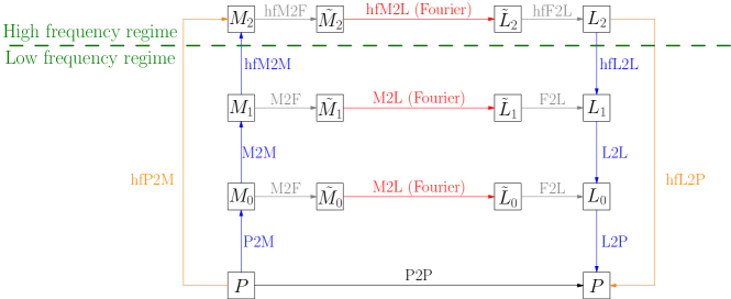
As described in section 2, the M2L application on equispaced grids involves three steps: the conversion of the involved multipole expansion (extended by zero-padding) into the Fourier domain, the application of the diagonal M2L operator in this domain, and then the conversion of the resulting (extended) local expansion in the Fourier domain into a local expansion. We thus introduce two extra operators, the M2F (multipole-to-Fourier) and F2L (Fourier-to-local) ones, applying the matrices $\mathbb{F}\chi$ to multipole expansions in the real domain and $\chi^{T}\mathbb{F}^{*}$ to local expansions in the Fourier domain. Let $T$ be a M2L matrix, we have (see section 2.3)

$$T=\underbrace{\left(\chi^{\top}\mathbb{F}^{*}\right)}_{\text{F2L}}\hskip 5.69046pt\underbrace{\mathbb{D}_{s,t}}_{\text{Diagonal M2L}}\hskip 5.69046pt\underbrace{\left(\mathbb{F}\chi\right)}_{\text{M2F}}.$$

In Figure 2, we depict how the different operators are applied in defmm. The operators are non-directional (i.e. without the terms in grey in section 2.2) in the low-frequency regime, and directional in the high-frequency one.

Figure 2: Operators and expansions in defmm. hf is added in front of the directional operators (used in the high-frequency regime). P: particles; $M_{i}$: multipole expansions; $L_{i}$: local expansions; $\tilde{M}_{i}$,$\tilde{L}_{i}$: multipole and local expansions in the Fourier domain.

4.1.2 Direction generation

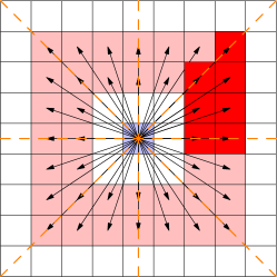
In the directional FMM presented in [15] the symmetries within the sets of directions at each tree level are exploited to reduce the number of precomputed M2L matrices. This however constrains the way the directions are generated. On the contrary, using a directional interpolation-based approach the M2L matrices do not depend on the directions (see section 2.2). We thus exploit a similar construction algorithm as presented in [15, 7]: starting from a given regular solid, the set of projected face centers on the unit sphere are chosen as directions at the first high-frequency level. Then, each face is subdivided into $2^{d-1}$ other faces and the process is repeated recursively in order to obtain the direction tree. Engquist & Ying [15] relies on the $d$-cube for the direction generation: according to our tests, the $d$-cube provides indeed the best compromise between the number of directions and the obtained accuracy among the platonic solids. Since, a $d$-cube has $d!$ faces, there are $d!2^{E(d-1)}$ directions at the $E^{th}$ high-frequency level in defmm.

4.2 Algorithmic design

4.2.1 $2^{d}$-tree construction

$2^{d}$-trees can be built either by setting the maximum number of particles per leaf (denoted as $Ncrit$), or by setting the maximum possible level (denoted as $MaxDepth$). For (highly) non-uniform particle distributions, the $MaxDepth$ strategy leads to (numerous) empty cells, which should not be stored and processed in practice: this requires advanced data structures (see e.g. [27, 13, 22]). The $MaxDepth$ strategy may also generate cells with a greatly varying number of particles [28]. Moreover, a comparison of hierarchical methods in [17] has detailed how the $Ncrit$ strategy better adapts to highly non-uniform distributions than the $MaxDepth$ one. Considering the highly non-uniform distributions used in BIE problems, we therefore choose to rely on the $Ncrit$ strategy in defmm. This differs from dfmm [25, 24] which relies on the $MaxDepth$ strategy.

Concretely, our $2^{d}$-tree construction algorithm is similar to the exafmm one: the particles are first sorted according to the Morton ordering, then each cell is built with a pointer on its first particle. The particles within a cell are thus stored consecutively in memory and followed by the particles of the next cell in the Morton ordering. This ensures that the data is localized for the P2P evaluations. In addition, since the particles of the sons of a given cell are stored consecutively, we can directly apply P2P operators on non-leaf cells. The charges and potentials are stored in two dedicated arrays whose entries correspond to the sorted particles for the same data-locality reason.

We also store all the directional expansions associated to a given cell $c$ in the same array to enhance data locality during the translations of local and multipole expansions: the M2M and L2L evaluations regarding $c$ are indeed performed alltogether (see section 5.2 for the optimizations of these steps).

4.2.2 Dual Tree Traversal

Algorithm 1 Dual Tree Traversal (DTT) between target cell $t$ and source cell $s$

1:  {$\mathcal{A}$: strict (resp. directional) MAC in low- (resp. high-) frequency regime}

2:  if $\mathcal{A}(t,s)$ then

3:     apply the M2L operator between $t$ and $s$

4:     return  

5:  else

6:     if $t$ is a leaf or $s$ is a leaf then

7:        apply the P2P operator between $t$ and $s$

8:        return  

9:     end if

10:     for $t^{\prime}\in Sons(t)$ do

11:        for $s^{\prime}\in Sons(s)$ do

12:           DTT($t^{\prime},s^{\prime}$)

13:        end for

14:     end for

15:  end if

Using the $Ncrit$ criterion however complexifies the interaction list structure (see lists U, V, W and X in e.g. [32]). In directional FMMs, the DPSC for well-separateness (see equation (4)) further complicates the construction of the interaction lists (multiple lists for each target cell with varying sizes and shapes depending on the tree level). We therefore adapt here the Dual Tree Traversal (DTT) [14, 33] to directional FMMs. The DTT is a simple and recursive procedure that simultaneously traverses the target and source trees to evaluate on-the-fly the M2L and P2P operators by dynamically testing the MAC on pairs of target and source cells. Hence, the interaction lists are traversed and evaluated implicitly but never built. This is another difference with dfmm which relies on a DTT-like algorithm to explicitly build the interaction lists during a precomputation step, and then separately processes these lists for each target cell.

Since FFTs can only efficiently accelerate M2L operations between cells at the same level (because of the relatively small involved circulant embedding), our DTT differs from the original one [14, 33] as follows: (i) when the MAC fails, both cells are split (not the largest one); (ii) a P2P operation is required as soon as one of the two cells is a leaf (not both).

We also aim at one single DTT algorithm for both the low- and high-frequency regimes. This requires the MAC to depend only on the cell radii and distances, and not on directions. Fortunately, this is possible in a directional polynomial interpolation-based FMM, since the M2L matrices do not depend on the directions. Our DTT hence relies in the low-frequency regime on the strict MAC (see section 4), which is simple and allows the most far-field interactions for each target cell, and on the following new directional MAC in the high-frequency regime (for wavenumber $\kappa$) between cells $t,s$ with radius $w$ at the same tree level:

$$\frac{max\{\kappa w^{2},2w\}}{dist(t,s)}\leq\eta,$$ (15)

where $\eta>0$ ($\eta=1$ in practice). This new directional MAC is similar to another directional MAC [7], but contrary to this latter our MAC does not depend on the directed wedge condition: we do not consider directions in this MAC but only ratios between cell radii and the cell distance. This means that the DTT performs in the high-frequency regime in a similar way than in the low-frequency one, without considering the directional aspects that are entirely hidden in the M2L applications. We emphasize that the interpolation process using equispaced grids is consistant according to section 3 on cells complying with these two MACs. When this directional MAC is satisfied, one then has to retrieve the best direction to select the directional multipole expansion (from source $s$) and the directional local expansion (from target $t$) which are relevant for the M2L operation between $t$ and $s$. The search of the best direction may have a non-negligible cost, but there is one single direction associated to each M2L matrix. We thus precompute these best directions during the M2L matrix precomputation step (see section 4.2.3).

In the end, we obtain the simple DTT algorithm presented in Algorithm 1 to differentiate in defmm the far-field M2L operations from the near-field P2P ones, in both low- and high-frequency regimes.

One may notice that list-based approaches (i.e. without DTT) allow to group or ”stack” multiple M2L operations (written as matrix-vector products), into matrix-matrix products (see e.g. [13, 24, 23]). This enables indeed to benefit from the higher efficiency of level-3 BLAS routines, especially for uniform distributions. We refer to this technique as vector stacking. Here however, we have M2L operations corresponding to Hadamard products whose grouping cannot lead to more efficient level-3 BLAS operations. Such Hadamard products may be converted to matrix-vector products as shown in [23], but this requires extra zeros for non-uniform particle distributions. Considering the highly non-uniform distributions typical of BIE problems, we believe that the potential gain would be too limited. We hence do not consider vector stacking for our Hadamard products, and we rather rely on the DTT to efficiently process the BIE non-uniform distributions.

4.2.3 Blank passes

Algorithm 2 Blank Dual Tree Traversal (BDTT) between target cell $t$ and source cell $s$

1:  if $t$ is in the high-frequency regime then

2:     if $\mathcal{A}(t,s)$ then

3:        {$\mathcal{D}(Level(t))$ is the level of $t$ in the direction tree:  }

4:        compute direction $u:=\displaystyle\mathop{argmin}_{v\in\mathcal{D}(Level(t))}\Big{|}v-\frac{ctr(t)-ctr(s)}{|ctr(t)-ctr(s)|}\Big{|}$

5:        mark $t$ and $s$ with $u$

6:        if the M2L matrix $\mathbb{D}_{s,t}$ corresponding to $t$ and $s$ is not precomputed then

7:           precompute $\mathbb{D}_{s,t}$

8:        end if

9:        mark $\mathbb{D}_{s,t}$ with $u$

10:        return  

11:     else

12:        for $t^{\prime}\in Sons(t)$ do

13:           for $s^{\prime}\in Sons(s)$ do

14:              BDTT($t^{\prime},s^{\prime}$)

15:           end for

16:        end for

17:     end if

18:  end if

Algorithm 3 Blank Downward Pass (BDP) for cell $c$

1:  if $c$ is in the high-frequency regime then

2:     for each direction $u$ with which $c$ is marked do

3:        for $c^{\prime}\in Sons(c)$ do

4:           mark $c^{\prime}$ with $Father(u)$

5:        end for

6:     end for

7:     for $c^{\prime}\in Sons(c)$ do

8:        BDP($c^{\prime}$)

9:     end for

10:  end if

On non-uniform distributions only a subset of all possible directional expansions will be used in practice due to the DPSC. Hence, defmm determines the actually needed directional expansions (named effective expansions) during a precomputation step and only computes and stores these effective expansions to save memory and computations. In this purpose, defmm performs first a blank DTT (see Algorithm 2) to compute each required M2L matrix and to mark all M2L-interacting cells with the corresponding direction (see line 5 in Algorithm 2). Then, thanks to a blank downward pass (see algorithm 3), the required directions are propagated down to the leaves of the $2^{d}$-trees.

4.3 Exploiting symmetries in the Fourier domain

To minimize the number of M2L matrices to be precomputed, in the case of centered expansions in $2^{d}$-trees, it has been observed in the literature that symmetries can be used (see for instance [24, 15]). The underlying symmetry group is actually the hyperoctahedral one [12] (i.e. the octahedral group in 3D, corresponding to the symmetry group of the cube), denoted by $\mathfrak{D}_{d}$ in dimension $d$, that can be realized as a group of rotation matrices. The use of symmetries strongly reduces the precomputation cost, especially in the high-frequency regime. Hence, we want to also exploit these symmetries in defmm. To do so, one has to express these symmetries in the Fourier domain, since the (modified diagonal) M2L matrices are expressed in this domain.

4.3.1 Taking symmetries into account

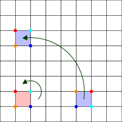
Let us first detail how, in a given cell $c$ of the (source or target) cluster tree, a permutation matrix over the interpolation grid $\Xi_{c}$ can be associated to a symmetry. Take any rotation $R:\mathbb{R}^{d}\to\mathbb{R}^{d}$ that leaves the unit cube centered at $0$ invariant. The set of rotations satisfying this property forms the so-called hyperoctahedral group. The translated grid $\Xi_{c}-ctr(c)$ is centered at the origin, so $\Xi_{c}-ctr(c)=R(\Xi_{c}-ctr(c))$ i.e. $\Xi_{c}=ctr(c)+R(\Xi_{c}-ctr(c))$. This transformation, represented in Figure 3, induces a linear map $\mathbb{R}_{c}:\mathbb{C}[\Xi_{c}]\to\mathbb{C}[\Xi_{c}]$ defined by

$$\mathbb{R}_{c}(u)(\mathbf{p}):=u(ctr(c)+R(\mathbf{p}-ctr(c)))$$ (16)

$$\forall u\in\mathbb{C}[\Xi_{c}],\;\forall\mathbf{p}\in\Xi_{c}.$$

This matrix $\mathbb{R}_{c}$ is a permutation of interpolation nodes, and the correspondence $R\leftrightarrow\mathbb{R}_{c}$ implements a permutation representation of the hyperoctahedral group. This is the group representation that we propose to exploit to minimize the number of precomputed M2L matrices.

Figure 3: Left: Source cell $s$ in the low-frequency regime (blue) with possible target cells $t$ (red) such that $s$ is in the interaction list of $t$. The corresponding M2L matrices for cells $t$ in pale red can be all deduced (for instance) from permutations of the dark red ones. Symmetry axes of the square ($2$-cube) are represented in orange. Middle and right: M2L matrix between the red and blue well-separated cells (middle) as a rotation of the M2L matrix between the red and grey cells (right), that permutes the relative positions of the interpolation nodes (colored dots). Since the entries of the M2L matrices correspond to interpolation nodes, permutations matrices represent this process. The underlying symmetry of $\mathfrak{D}_{2}$ is the reflection with regard to the line $x=y$.

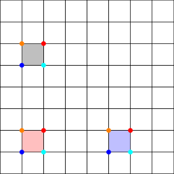
Denote $\mathbb{R}_{\star}:\mathbb{C}[\Xi_{\star}]\to\mathbb{C}[\Xi_{\star}]$ the permutation induced on $\Xi_{\star}$ by means of the correspondence described above. When the same rotation transformation is applied to both source and target cells $s$ and $t$, the transformed M2L matrix writes

$$\mathbb{R}_{t}^{\top}G(\Xi_{t},\Xi_{s})\mathbb{R}_{s} =\mathbb{R}_{\star}^{\top}\mathcal{G}_{s,t}(\Xi_{\star},\Xi_{\star})\mathbb{R}_{\star}$$ (17)

$$=\mathbb{R}_{\star}^{\top}\chi^{\top}\mathbb{F}^{*}\mathbb{D}_{s,t}\mathbb{F}\chi\mathbb{R}_{\star}.$$

We are going to show that the product above actually writes $\chi^{\top}\mathbb{F}^{*}\tilde{\mathbb{D}}_{s,t}\mathbb{F}\chi$ where $\tilde{\mathbb{D}}_{s,t}$ is a diagonal matrix mapping $\mathbb{C}[\widehat{\Xi}_{\star}]\to\mathbb{C}[\widehat{\Xi}_{\star}]$ with coefficients obtained by permuting the diagonal of $\mathbb{D}_{s,t}$.

In concrete computational terms, this means that, whenever two M2L interactions only differ by a rotation, one M2L matrix is deduced from the other by a simple permutation of the diagonal entries of the factor term $\mathbb{D}_{s,t}$, which reduces storage and precomputation cost.

Let $c_{\star}=(1/2,\dots,1/2)=ctr(\Xi_{\star})\in\mathbb{R}^{d}$ refer to the center of the normalized interpolation grid. Denote $\Xi_{0}=\Xi_{\star}-ctr(\Xi_{\star})$ the normalized interpolation grid translated so as to be centered at $0$. Take two vectors $u,v\in\mathbb{C}[\Xi_{\star}]$. Then we have

$$v^{\top}\mathbb{R}_{\star}^{\top}\mathcal{G}_{s,t}(\Xi_{\star},\Xi_{\star})\mathbb{R}_{\star}u$$ (18)

$$=\sum_{\mathbf{p}\in\Xi_{\star}}\sum_{\mathbf{q}\in\Xi_{\star}}\mathcal{G}_{s,t}(\mathbf{p}-\mathbf{q})u(c_{\star}+R(\mathbf{p}-c_{\star}))v(c_{\star}+R(\mathbf{q}-c_{\star}))$$

$$=\sum_{\mathbf{x}\in\Xi_{0}}\sum_{\mathbf{y}\in\Xi_{0}}\mathcal{G}_{s,t}(\mathbf{x}-\mathbf{y})u(c_{\star}+R(\mathbf{x}))v(c_{\star}+R(\mathbf{y}))$$

$$=\sum_{\mathbf{x}^{\prime}\in\Xi_{\star}}\sum_{\mathbf{y}^{\prime}\in\Xi_{\star}}\mathcal{G}_{s,t}(R^{*}(\mathbf{p}-\mathbf{q}))u(\mathbf{p})v(\mathbf{q}).$$

Since $u,v$ are arbitrarily chosen in $\mathbb{C}[\Xi_{\star}]$, this can be rewritten in condensed form by $\mathbb{R}_{\star}^{\top}\mathcal{G}_{s,t}(\Xi_{\star},\Xi_{\star})\mathbb{R}_{\star}=(\mathcal{G}_{s,t}\circ R^{*})(\Xi_{\star},\Xi_{\star})$. Now there only remains to return to the calculus presented in section 2.3 that shows

$$\mathbb{R}_{\star}^{\top}\mathcal{G}_{s,t}(\Xi_{\star},\Xi_{\star})\mathbb{R}_{\star}=\chi^{\top}\mathbb{F}^{*}\,\mathbb{D}[\mathcal{G}_{s,t}\circ R^{*}]\,\mathbb{F}\chi$$ (19)

$$\text{with}\quad\mathbb{D}[\mathcal{G}_{s,t}\circ R^{*}]=\mathrm{diag}(\,\mathbb{F}(\mathcal{G}_{s,t}\circ R^{*})\,).$$

To summarize, the only difference between $\mathbb{R}_{\star}^{\top}\mathcal{G}_{s,t}(\Xi_{\star},\Xi_{\star})\mathbb{R}_{\star}$ and $\mathcal{G}_{s,t}(\Xi_{\star},\Xi_{\star})$ lies in the coefficients of the Fourier symbol in the central diagonal term of their factorized form. Let us examine how the rotation $R^{*}$ acts on the Fourier symbol of $\mathcal{G}_{s,t}$. According to (12), and since $R(\Xi_{\sharp})=\Xi_{\sharp}$, we have

$$\mathbb{F}(\mathcal{G}_{s,t}\circ R^{*})(\boldsymbol{\xi}) =\frac{1}{T^{d/2}}\sum_{\mathbf{x}\in\Xi_{\sharp}}\mathcal{G}_{s,t}(R^{*}\mathbf{x})\exp(-2\imath\pi\,\boldsymbol{\xi}\cdot\mathbf{x})$$ (20)

$$=\frac{1}{T^{d/2}}\sum_{\mathbf{y}\in\Xi_{\sharp}}\mathcal{G}_{s,t}(\mathbf{y})\exp(-2\imath\pi\,R^{*}(\boldsymbol{\xi})\cdot\mathbf{y})=\mathbb{F}(\mathcal{G}_{s,t})(R^{*}\boldsymbol{\xi})$$

which again summarizes as $\mathbb{F}(\mathcal{G}_{s,t}\circ R^{*})=\mathbb{F}(\mathcal{G}_{s,t})\circ R^{*}$. In other words, the permutation on the grid $\widehat{\Xi}_{\sharp}$ that should be applied on the symbol of the periodized M2L operator is the permutation associated to the inverse rotation $R^{*}=R^{-1}$.

4.3.2 Symmetries in practice

Usually, the multipole and local expansions are permuted respectively before and after the evaluation of a M2L operator (see e.g. [24, 23]). Here we can reduce this number of applied permutations to only one thanks to the diagonal form of the M2L matrices in the Fourier domain in defmm (see equation (19)). Indeed, the permutations can all be applied to these diagonal M2L matrices, resulting in a permutation of their diagonal entries. This reduces the number of permutations from two to only one.

In practice, the permutations induce memory indirections when performing the Hadamard products that may prevent the compiler auto-vectorization. We hence rely on an OpenMP directive to enforce the compiler vectorization (see [12] for details).

5 Optimizations

We here present algorithmic and programming optimizations regarding high performance computing on one CPU core.

5.1 Processing the FFTs

Figure 4: Timings of all FFT applications with 1D interpolation order $4$, using the batch and individual methods. Tests performed with $10^{7}$ particles (see section 6 for details).

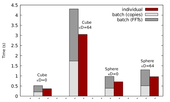
We rely on the state-of-the-art FFTW library [18] to efficiently perform all at once our numerous FFTs. Our 3D FFTs (considering $d=3$) are however small: $(2L-1)^{d}$ elements, with usually $L\leq 7$. This makes the FFTW ”plan” creation, required to decide the most efficient FFT implementation, more time consuming than its execution (i.e. the actual FFT computation). Moreover, zero-padding is required for the circulant embedding (see section 4.3) of the expansions stored in the Fourier domain: this implies expansion copies before each FFT, as well as after each reverse FFT.

One could first use the ”batch” FFTW feature to efficiently process our numerous small FFTs. This performs all FFTs with one single FFTW plan and can improve performance compared to multiple individual FFT calls. All expansion copies hence have to be performed all together before and after the batch FFTW call. We refer to this method as the batch one.

Since all our expansions have the same size and the same memory alignment, we can also rely on one single FFTW plan for all our FFTs, and perform individually each FFT along with its expansion copy. This individual method benefits from the cache memory for our small-sized expansions, and hence avoids to load data twice from main memory (for FFTs and for copies, which are both memory-bound operations) as done in the batch method. This is shown in figure 4, where the individual method always outperforms (up to 30%) the batch one. We thus use the individual method in defmm.

5.2 BLAS-based upward and downward pass operators

Because of the directional aspects of defmm, the cost of the upward and downward passes is linearithmic for surface meshes (see [15]). As opposed to FMMs for non-oscillatory kernels, these steps have a significant cost in practice, which justifies their careful optimization. We hence first adapt an optimization suggested in [2] to equispaced grids and to oscillatory kernels (see section 5.2.1), and then improve it for directional FMMs (see sections 5.2.2 and 5.2.3). We validate our optimizations in section 5.2.4.

5.2.1 Tensorized M2M and L2L operators

We here detail a fast evaluation scheme suggested in [2] for the M2M and L2L operators on interpolation grids using tensorized Chebyshev rules in the low-frequency regime. We extend this scheme to equispaced grids which are also tensorized grids. The bijection in definition 1 induces a node indexing in the interpolation grid $\mathbb{G}$ allowing to exploit this tensorized structure.

Definition 1.

Let $L\in\mathbb{N}$. $\mathfrak{I}$ denotes the bijection from $[\![0,L^{d}-1]\!]$ to $[\![0,L-1]\!]^{d}$ such that $\mathfrak{I}^{-1}(\mathbf{I}):=\sum_{k=1}^{d}I_{k}L^{k-1}$, $\forall\hskip 2.84544pt\mathbf{I}:=\left(\mathfrak{I}_{1},...,\mathfrak{I}_{d}\right)$.

Thanks to this tensorized structure, the matrix representations of the M2M and L2L operators are tensorized matrices. The L2L case being obtained by transposition, we focus on the M2M case. Let $\mathbb{M}\in\mathbb{R}^{L^{d}\times L^{d}}$ be the matrix representation of a M2M operation, there exists therefore $M^{(p)}\in\mathbb{R}^{L\times L}$, $p\in[\![1,d]\!]$, such that $\mathbb{M}=\displaystyle\mathop{\otimes}_{p=1}^{d}M^{(p)}$. Using definition 1, the following holds

$$\left(\mathop{\otimes}_{k=1}^{d}M^{(k)}\right)_{i,j}=\prod_{k=1}^{d}M^{(k)}_{\mathfrak{I}(i)_{k},\mathfrak{I}(j)_{k}}.$$

For any $\mathbf{v}\in\mathbb{C}^{L^{d}}$, we have

$$\left(\mathbb{M}\mathbf{v}\right)_{i} =\left(\left(\mathop{\otimes}_{k=1}^{d}M^{(k)}\right)\mathbf{v}\right)_{i}=\sum_{j=0}^{L^{d}-1}\left(\mathop{\prod}_{p=1}^{d}M^{(p)}_{\mathfrak{I}(i)_{p},\mathfrak{I}(j)_{p}}\right)v_{j}$$

$$=\sum_{\mathbf{J}\in[\![0,L-1]\!]^{d}}\mathop{\prod}_{p=1}^{d}M^{(p)}_{\mathfrak{I}(i)_{p},\mathbf{J}_{p}}v_{\mathfrak{I}^{-1}(\mathbf{J})}=\sum_{\mathbf{J}\in[\![0,L-1]\!]^{d}}\mathop{\prod}_{p=1}^{d-1}M^{(p)}_{\mathfrak{I}(i)_{p},\mathbf{J}_{p}}\left(M^{(d)}_{\mathfrak{I}(i)_{d},\mathbf{J}_{d}}v_{\mathfrak{I}^{-1}(\mathbf{J})}\right)$$

$$=\sum_{\begin{subarray}{c}\mathbf{J}\in[\![0,L-1]\!]^{d}\\ \mathbf{J}_{d}=0\end{subarray}}\mathop{\prod}_{p=1}^{d-1}M^{(p)}_{\mathfrak{I}(i)_{p},\mathbf{J}_{p}}\left(\sum_{q=0}^{L-1}M^{(d)}_{\mathfrak{I}(i)_{d},q}v_{\mathfrak{I}^{-1}(\mathbf{J}+q\mathbf{e}_{d})}\right)$$

where the last sum over $q$ matches a matrix-vector product of size $L\times L$. For $i$ varying, this matrix-vector product is performed on $L^{d-1}$ different restrictions of $\mathbf{v}$, involving each time the same matrix. Hence, there exists a permutation $P\in\mathbb{R}^{L^{d}\times L^{d}}$ such that

$$\left(\mathbb{M}\mathbf{v}\right)_{i} =\sum_{\begin{subarray}{c}\mathbf{J}\in[\![0,L-1]\!]^{d}\\ \mathbf{J}_{d}=0\end{subarray}}\mathop{\prod}_{p=1}^{d-1}M^{(p)}_{\mathfrak{I}(i)_{p},\mathbf{J}_{p}}\left(diag(M^{(d)})P\mathbf{v}\right)_{\mathfrak{I}(i)_{d}}$$

where $diag(M^{(d)})$ is a block-diagonal matrix with all diagonal bocks equal to $M^{(d)}$. This process can be repeated $d$ times, leading to an overall complexity of $\mathcal{O}\left(dL^{d+1}\right)$ since the permutations are applied in $\mathcal{O}(L^{d})$ operations. This compares favorably with the $\mathcal{O}\left(L^{2d}\right)$ complexity of a naive approach. Since the same matrix is used for multiple vectors at each of the $d$ iterations, matrix-vector products can be stacked into matrix-matrix products to benefit from the level-3 BLAS higher efficiency [2]. We will refer to this version as the tensorized (or $t$) method.

The extension of the tensorized method to oscillatory kernels is obtained by noting that the directional M2M matrix $\mathbb{M}(u)$ with direction $u$ can be written

$$\mathbb{M}\left(u\right)=D_{0}(u)\left(\mathop{\otimes}_{p=1}^{d}M^{(p)}\right)D_{1}(u)$$ (21)

with two diagonal matrices $D_{0}(u)$ and $D_{1}(u)$ composed of complex exponential evaluations (see section 2.2).

5.2.2 Directional stacking

The tensorized method can be further optimized in the high-frequency regime. Starting from equation 21, if we consider for a given cell two directions $u$ and $u^{\prime}$ with corresponding directional multipole expansions $\mathbf{v}(u)$ and $\mathbf{v}(u^{\prime})$, denoting by $\odot$ the Hadamard product, the ”stacking”

$$\begin{bmatrix}\mathbb{M}(u)\mathbf{v}(u)&\mathbb{M}(u^{\prime})\mathbf{v}(u^{\prime})\end{bmatrix}$$

can be expressed as

$$\begin{bmatrix}D_{0}(u)&D_{0}(u^{\prime})\end{bmatrix}\odot\left(\left(\displaystyle\mathop{\otimes}_{p=1}^{d}M^{(p)}\right)\cdot\left(\begin{bmatrix}D_{1}(u)&D_{1}(u^{\prime})\end{bmatrix}\odot\begin{bmatrix}\mathbf{v}(u)&\mathbf{v}(u^{\prime})\end{bmatrix}\right)\right).$$

$\mathop{\otimes}_{p=1}^{d}M^{(p)}$ here applies to a matrix instead of a vector, which allows to further benefit from the level-3 BLAS efficiency. Contrary to the tensorized method where $L^{d-1}$ vectors can be stacked, the number of vectors that can be stacked is now $L^{d-1}$ multiplied by the number of effective directional multipole expansions in each cell. This method is referred to as the tensorized+stacking method (denoted $t+s$).

5.2.3 Benefiting from real matrix products

One may observe that the matrices $M^{(p)}$ are real since they are composed of evaluations of Lagrange polynomials, but are applied to complex vectors (at least in a directional method). For any $\mathbf{v}\in\mathbb{C}^{L^{d}}$, we thus have

$$\left(\mathop{\otimes}_{p=1}^{d}M^{(p)}\right)\mathbf{v} =\left(\mathop{\otimes}_{p=1}^{d}M^{(p)}\right)\mathfrak{Re}\{\mathbf{v}\}+i\left(\mathop{\otimes}_{p=1}^{d}M^{(p)}\right)\mathfrak{Im}\{\mathbf{v}\}.$$

By deinterleaving the real and imaginary parts in the expansion vectors, one can obtain stacked matrices of real elements. Hence, by discarding the imaginary part of the (real) M2M matrices, we can halve the number of required arithmetic operations. This method is referred to as the tensorized+stacking+real method (denoted $t+s+r$). Since there is only one multipole and one local expansion per cell in the low-frequency regime, no stacking of the directional expansions is performed and the $t+s+r$ method is reduced to $t+r$ in this frequency regime.

5.2.4 Performance results

(a) Sphere $\kappa D=0$

(b) Sphere $\kappa D=64$

(c) Cube $\kappa D=0$

(d) Cube $\kappa D=64$

Figure 5: Timings of all M2M evaluations for the tensorized ($t$), tensorized+stacking ($t+s$) and tensorized+stacking+real ($t+s+r$) methods, for different distributions with $10^{7}$ particles and for different frequency regimes. $\kappa D$ refers to the length of the particle distribution multiplied by the wavenumber $\kappa$. 1D interpolation orders are indicated inside parentheses. lfM2M (respectively hfM2M) refers to the low- (resp. high-) frequency M2M operations. See section 6.2 for a detailed test case description.

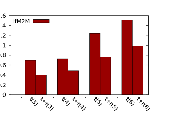
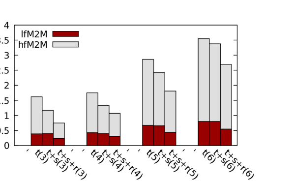
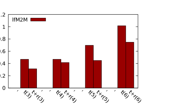
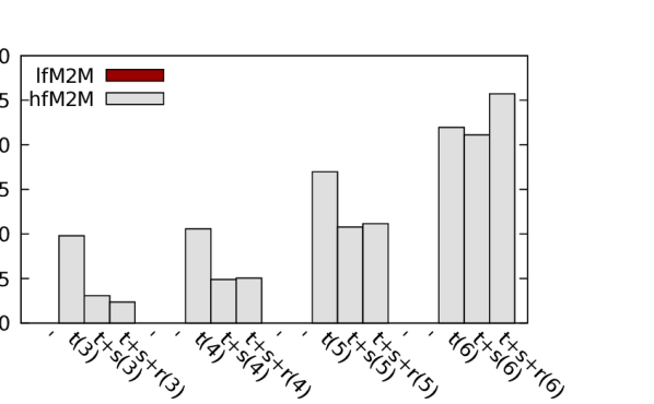
In figure 5 are detailed the M2M timings for these three optimizations. Regarding the sphere with $\kappa D=64$ (see figure 5(b)), the new $t+s$ method fastens the M2M evaluations of the $t$ method in the high-frequency regime, while our $t+s+r$ method further reduces the M2M evaluation times of this $t+s$ method in the two frequency regimes. In the end, our $t+s+r$ method outperforms the original $t$ method of [2] by a factor up to $2.16\times$.

This is also valid for the cube with $\kappa D=64$ (see figure 5(d)), when considering low interpolation orders: for $L=3$ the $t+s+r$ method outperforms the $t$ one by a factor of $\approx 4\times$. For larger interpolation orders, the $t+s+r$ method is however less efficient than the $t+s$ one, and even leads to a performance loss for $L=6$. This is due to our small matrix sizes (one matrix being of size $L\times L$) for which the $t+s$ method already provides a high enough number of stacked vectors with the cube distribution: there is thus no benefit with a higher number of stacked vectors (as provided by the $t+s+r$ method). Moreover, the deinterleaving cost is not here offset by the lower number of operations induced by the real matrix products.

In the low-frequency regime (see figures 5(a),5(b),5(c)), the deinterleaving still allows faster M2M evaluations than the original $t$ method with performance gains up to 4x. Since we target surface particle distributions for BIE problems, we choose to rely on the $t+s+r$ method in defmm for M2M evaluations, as well as for L2L ones (for which the same performance gains have been obtained).

5.3 Vectorization for direct computation

The direct computation involved in the P2P operator consists in two nested loops over the (possibly distinct) target and source particles. As usually performed in FMM codes, we aim at vectorizing this computation to benefit from the AVX2 or AVX-512 units. We target here the vectorization of the outer loop (on target particles), which leads to fewer reduction operations than with an inner loop vectorization. Based on the data locality among particles described in section 4.2.1, our P2P code is close to the one presented in [1]. As in [1], we load separately the real and imaginary parts of the complex numbers and we perform only real (not complex) mathematical operations: this is required for our compiler (Intel C++ compiler) to fully vectorize the code. There are nevertheless some differences between our code and the one presented in [1]:

• Since the inputs of our code are the particle point clouds, we have to be able to numerically handle the practical case of interactions between equally located particles on which the kernel function cannot be evaluated. These singularities (i.e. the interactions between a particle and itself) are resolved directly: if the distance between the particles is too small, we set one operand to $0.0$ and we continue the interaction computation, which hence results in $0.0$. This minimal test may be processed with masks in the vectorized code, hence leading to a minimal performance penalty.

• In order to vectorize our outer loop, an OpenMP compiler directive is required for the Intel C++ compiler (which targets the inner loop otherwise). It can be noticed that the GNU C++ compiler currently fails to vectorize our code (with or without the OpenMP directive).

• Since the particle positions are not updated from one FMM application to the next in BIE problems, we can rely on a structure-of-array data layout for the potentials and the charges, which favors efficient vector memory accesses.

In the end, using 64-bit floating-point numbers on 512-bit AVX-512 units (hence a maximum speedup of $8\times$), our vectorized P2P operator offers performance gains up to $7.6\times$ over the original scalar implementation (see [12] for details).

6 Numerical results

We now provide numerical results illustrating the convergence and the performance of defmm. All codes run sequentially on a Intel Xeon Gold 6152 CPU with AVX-512 units and 384 GB of RAM.

6.1 Relative error

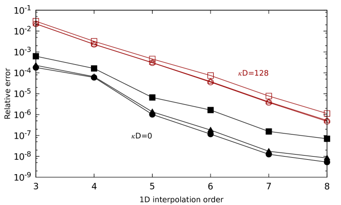
We first check the overall accuracy of defmm on a (volumic) uniform cube test case composed of $125000$ particles. We compute the error of a defmm approximation $\tilde{p}$ of $p$ (see equation (1)) for a norm $||\cdot||$ as $\frac{||p-\tilde{p}||}{||p||}$. The charges are randomly chosen.

As shown in figure 6, the convergence follows the estimate derived from the interpolation process on equispaced grids in section 3.2, i.e. a geometric convergence in the 1D interpolation order. However, the same interpolation order leads to lower accuracies in the high-frequency regime than in the low-frequency one. We believe that this is a consequence of the small initial set of directions chosen for performance reasons in the defmm implementation (see section 4.1.2). Similar results were obtained on a surface sphere distribution.

Figure 6: Relative error of the FMM over a 3D uniform cube with $1.25\times 10^{5}$ particles. Maximum norm: squares; $l^{1}$ norm: circles; $l^{2}$ norm: triangles.

6.2 Performance comparison with dfmm

For this performance comparison, we consider the following test cases, all with $10^{7}$ particles ($\pm 1\%$).

• The uniform cube test case (volumic distribution). This classical FMM test case is not typical for BIE problems, but is still interesting due to its high computation cost for directional FMMs (the number of effective expansions being maximum).

• The classical sphere test case where the particles are quasi-uniformly scattered on the surface of the unit sphere. This is also considered as a difficult case, with high memory requirements and high computation costs, for the directional methods on boundary particle distributions [15].

• The refined cube, where the particles are highly non-uniformly sampled along the surface of the unit cube with a higher concentration around the edges and corners. This mimics distributions obtained with mesh refinement.

• The ellipse, which is an elongated distribution favorable to directional FMMs due to the reduced number of directions in the high-frequency regime. Our ellipse distribution presents a higher concentration of particles on the two poles.

defmm is compiled using the Intel C++ compiler. All the BLAS calls use the Intel Math Kernel Library (MKL) and we rely on the FFTW3 library for the FFTs.

Regarding dfmm (only g++ supported), we consider its two best variants [24], both based on low-rank compressions and on interpolations using tensorized Chebyshev grids. The first variant (IAblk – Individual Approximation with symmetries and BLocKing) relies on vector stacking and symmetries to improve performance with level-3 BLAS routines. The second one (SArcmp – Single Approximation with ReCoMPression) uses global approximations of the M2L matrices and recompressions to reduce the numerical ranks of these matrices. According to [24], this can lead to faster M2L evaluations than with IAblk, but at the cost of longer precomputation times.

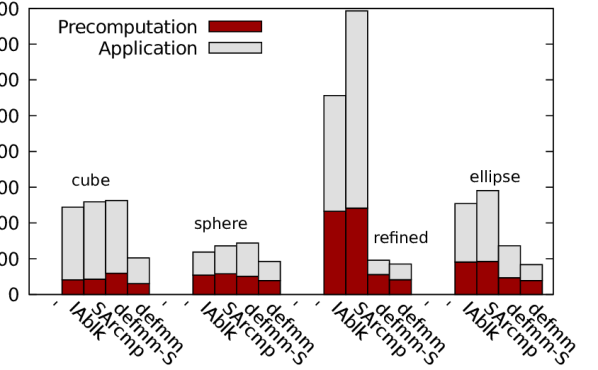
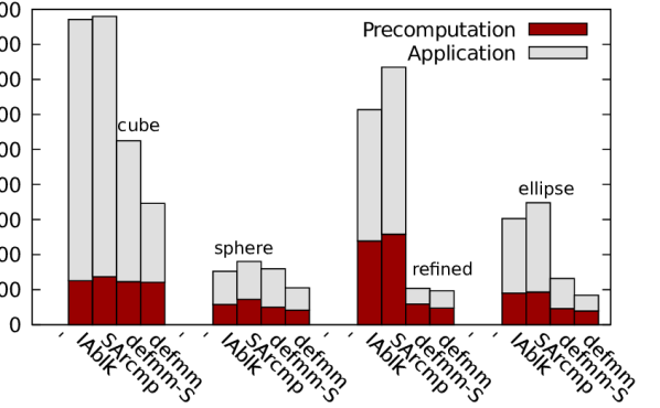
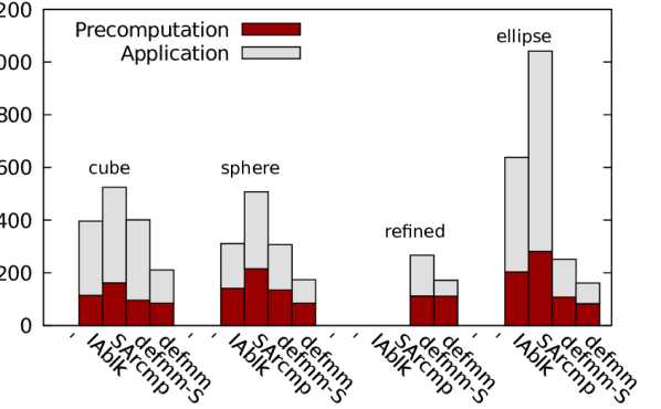
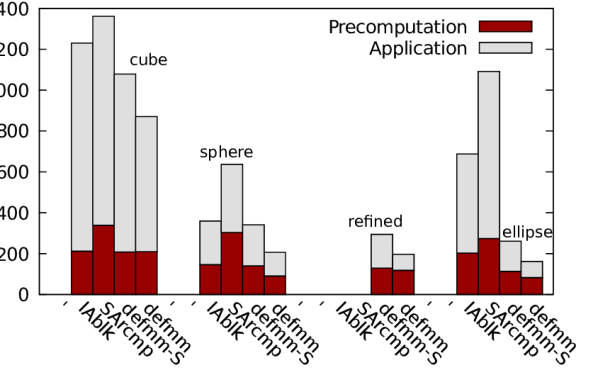
Following the methodology used in [25], we fix the threshold in the low-rank approximations of dfmm to $10^{-L}$. We checked that the accuracy of the Chebyshev interpolation in dfmm is then similar to the accuracy of the equispaced interpolation in defmm. For each test, the $MaxDepth$ (dfmm) and the $Ncrit$ (defmm) values (see section 4.2.1) are tuned to minimize the FMM application time. Due to memory constraints, we were not able to run dfmm (with IAblk or SArcmp) on the refined cube for $L=6$. The comparison results are given in figure 7.

(a) $L=4$, $\kappa D=0$

(b) $L=4$, $\kappa D=64$

(c) $L=6$, $\kappa D=0$

(d) $L=6$, $\kappa D=64$

Figure 7: Timings for one FMM execution of the dfmm and defmm variants. The two tested variants of dfmm are IAblk and SArcmp. defmm-S corresponds to defmm without P2P vectorization.

Overall performance

Considering the overall times (including precomputation and application times), defmm always outperforms dfmm, being $1.3\times$ to $6.5\times$ faster than its best variant (IAblk here). As detailed below, this is due to the different design of the two codes. Since the P2P operator is not vectorized in dfmm, we also present in figure 7 a defmm variant, denoted by defmm-S, with a scalar (i.e. non-vectorized) P2P implementation. This enables us to more precisely study the impact of the other differences between defmm and dfmm. defmm-S offers similar or better performance than the best dfmm variant on the uniform cube and on the sphere, and outperforms dfmm by factors $1.8\times$ to $5.9\times$ on more non-uniform distributions (i.e. the refined cube and the ellipse). This shows that regarding directional FMMs our FFT-based approach is competitive with or faster than the low-rank approximations used in dfmm.

Sensitivity to the particle distribution

Since the distributions have the same number of particles ($\pm 1\%$), comparing two distributions (all other test parameters being identical) illustrates the sensitivity of the method to the particle distribution. Except for the uniform cube in the high-frequency regime (whose higher cost is due to its maximum number of effective directional expansions), the defmm performance is few sensitive to the distribution, contrary to the dfmm one. This is due to the differences in the tree construction and traversal (see section 4.2): the combination of the $Ncrit$ strategy and of our specific DTT allows to better adapt in defmm to the particle distribution than the $MaxDepth$ strategy used in dfmm. Besides, the performance gap between IAblk and defmm-S is minimized for the (uniform) cube and the sphere (quasi-uniform on its surface) distributions. These two distributions benefit indeed most from the BLAS routines and from the vector stacking in IAblk.

Sensitivity to the wavenumber

Since both codes are based on the same directional approach, their performance is similarly impacted by an increase in the wavenumber. Again, the uniform cube in the high-frequency regime is a special case (maximizing the number of effective expansions), where the dfmm features (level-3 BLAS routines, cache management) lower here the performance gap with defmm when the wavenumber increases: dfmm is however still outperformed by defmm in this case.

Sensitivity to the interpolation order

When moving from $L=4$ to $L=6$, the average performance ratio of defmm-S over SArcmp moves from $1.58\times$ to $2.40\times$ (for the uniform cube, the sphere and the ellipse test cases, and for any frequency). This increasing performance gain with respect to the interpolation order is due to our FFT-based FMM. With respect to IAblk, the performance gain of defmm-S moves from $1.42\times$ to $1.56\times$: here the FFT gain is counterbalanced by the BLAS performance gain (which is greater for larger matrices).

Precomputation costs

Thanks to our extension of the symmetry usage to the Fourier domain (see section 4.3), we manage to have on the uniform cube and on the sphere precomputation costs in defmm as low as the dfmm ones (considering the IAblk variant which requires shorter precomputations than SArcmp). In addition, in highly non-uniform distributions such as the refined cube and the ellipse, the precomputation costs of defmm are drastically lower than the dfmm ones, partly thanks to our $Ncrit$-based $2^{d}$-trees and to our blank passes (see section 4.2) which minimize the required precomputations.

7 Conclusion

In this paper we presented a new approach for the directional interpolation-based FMMs, using FFT techniques thanks to equispaced grids. We provided a consistency proof of the approximation process and showed how to extend the symmetries of the interpolation-based FMM to the Fourier domain. We detailed the algorithmic design of our defmm library, as well as its high-performance optimizations on one CPU core. Finally, a comparison with a state-of-the-art library exhibited the superior performance of our library in all test cases and in both high- and low-frequency regimes, the defmm performance being also few sensitive to the surface particle distribution.

Future works will be dedicated to the defmm parallelization. In this purpose, we will be able to lean on the dual tree traversal, which is known to be highly efficient regarding shared-memory parallelism (see e.g. [33, 1]), and on previous work (such as [4]) regarding distributed-memory parallelism. We also plan to integrate defmm in an iterative solver in order to solve complex realistic boundary integral equations.

References

- [1] M. Abduljabbar, M. A. Farhan, N. Al-Harthi, R. Chen, R. Yokota, H. Bagci, and D. Keyes, Extreme scale fmm-accelerated boundary integral equation solver for wave scattering, SIAM Journal on Scientific Computing, 41 (2019), pp. C245–C268.
- [2] E. Agullo, B. Bramas, O. Coulaud, E. Darve, M. Messner, and T. Takahashi, Pipelining the Fast Multipole Method over a Runtime System, Research Report RR-7981, INRIA, May 2012. https://hal.inria.fr/hal-00703130/file/RR-7981.pdf.
- [3] L. V. Ahlfors, Complex analysis: An introduction to the theory of analytic functions of one complex variable; 3rd ed., (1978), pp. xi+331.
- [4] A. R. Benson, J. Poulson, K. Tran, B. Engquist, and L. Ying, A parallel directional fast multipole method, SIAM J. Sci. Comput., 36 (2014), p. C335–C352.
- [5] P. Blanchard, O. Coulaud, and E. Darve, Fast hierarchical algorithms for generating Gaussian random fields, Research Report 8811, Inria Bordeaux Sud-Ouest, Dec. 2015.
- [6] A. Brandt, Multilevel computations of integral transforms and particle interactions with oscillatory kernels, Comput. Phys. Comm., 65 (1991), pp. 24–38.
- [7] S. Börm, Directional H2-matrix compression for high-frequency problems, Numer. Linear Algebra Appl., 24 (2017).
- [8] S. Börm and L. Grasedyck, Low-Rank Approximation of Integral Operators by Interpolation, Computing, 72 (2004), pp. 325–332.
- [9] C. Cecka and E. Darve, Fourier-based Fast Multipole Method for the Helmholtz equation, SIAM J. Sci. Comput., 35 (2013), p. A79–A103.
- [10] C. Chen, S. Aubry, T. Oppelstrup, A. Arsenlis, and E. Darve, Fast algorithms for evaluating the stress field of dislocation lines in anisotropic elastic media, Modelling and Simulation in Materials Science and Engineering, 26 (2018), p. 045007.
- [11] H. Cheng, W. Y. Crutchfield, Z. Gimbutas, L. F. Greengard, J. F. Ethridge, J. Huang, V. Rokhlin, N. Yarvin, and J. Zhao, A wideband fast multipole method for the Helmholtz equation in three dimensions, J. Comput. Phys., 216 (2006), p. 300–325.
- [12] I. Chollet, Symmetries and Fast Multipole Methods for Oscillatory Kernels, Ph.D. thesis, Sorbonne Université, Mar. 2021, https://tel.archives-ouvertes.fr/tel-03203231.
- [13] O. Coulaud, P. Fortin, and J. Roman, High-performance BLAS formulation of the adaptive Fast Multipole Method, Mathematical and Computer Modelling, 51 (2010), pp. 177–188.
- [14] W. Dehnen, A hierarchical O(N) force calculation algorithm, J. Comput. Phys., 179 (2002), p. 27–42.
- [15] B. Engquist and L. Ying, Fast directional multilevel algorithms for oscillatory kernels, SIAM Journal on Scientific Computing, 29 (2007), p. 1710–1737.
- [16] W. Fong and E. Darve, The black-box fast multipole method, J. Comput. Phys., 228 (2009), pp. 8712–8725.
- [17] P. Fortin, E. Athanassoula, and J.-C. Lambert, Comparisons of different codes for galactic N-body simulations, Astronomy and Astrophysics - A&A, 531 (2011), p. A120.
- [18] M. Frigo and S. G. Johnson, The design and implementation of FFTW3, Proceedings of the IEEE, 93 (2005), pp. 216–231. Special issue on “Program Generation, Optimization, and Platform Adaptation”.
- [19] M. Gasca and T. Sauer, Polynomial interpolation in several variables, Advances in Computational Mathematics, 12 (2000), pp. 377–410.
- [20] K. Gibermann, Multilevel Approximation of Boundary Integral Operators, Computing, 67 (2001), p. 183–207.
- [21] L. Greengard and V. Rokhlin, A fast algorithm for particle simulations, J. Comput. Phys., 73 (1987), pp. 325–348.
- [22] B. Hariharan, S. Aluru, and B. Shanker, A Scalable Parallel Fast Multipole Method for Analysis of Scattering from Perfect Electrically Conducting Surfaces, in SC ’02: Proceedings of the 2002 ACM/IEEE Conference on Supercomputing, 2002, pp. 42–42.
- [23] D. Malhotra and G. Biros, Algorithm 967: A Distributed-Memory Fast Multipole Method for Volume Potentials, ACM Trans. Math. Software, 43 (2016).
- [24] M. Messner, B. Bramas, O. Coulaud, and E. Darve, Optimized M2L kernels for the Chebyshev interpolation based fast multipole method, (2012). https://arxiv.org/abs/1210.7292.
- [25] M. Messner, M. Schanz, and E. Darve, Fast directional multilevel summation for oscillatory kernels based on Chebyshev interpolation, J. Comput. Phys., 231 (2012), p. 1175–1196.
- [26] B. Mößner and U. Reif, Error bounds for polynomial tensor product interpolation, Computing, 86 (2009), pp. 185–197.
- [27] K. Nabors, F. T. Korsmeyer, F. T. Leighton, and J. White, Preconditioned, Adaptive, Multipole-Accelerated Iterative Methods for Three-Dimensional First-Kind Integral Equations of Potential Theory, SIAM J. Sci. Comput., 15 (1994), p. 713–735.
- [28] V. Pavlov, N. Andonov, and G. Kremenliev, Porting and Verification of ExaFMM Library in MIC Architecture, (2014). https://doi.org/10.5281/zenodo.822725.
- [29] R. B. Platte, L. N. Trefethen, and A. B. J. Kuijlaars, Impossibility of fast stable approximation of analytic functions from equispaced samples, SIAM Review, 53 (2011), pp. 308–318.
- [30] D. Schobert and T. Eibert, A multilevel interpolating fast integral solver with fast Fourier Transform acceleration, Symposium Digest - 20th URSI International Symposium on Electromagnetic Theory, EMTS 2010, (2010), pp. 520 – 523.
- [31] S. Smith, Lebesgue constants in polynomial interpolation, Annales Mathematicae et Informaticae, 33 (2006), pp. 109–123.
- [32] L. Ying, G. Biros, and D. Zorin, A kernel-independent adaptive fast multipole algorithm in two and three dimensions, J. Comput. Phys., 196 (2004), p. 591–626.
- [33] R. Yokota, An FMM based on dual tree traversal for many-core architectures, Journal of Algorithms & Computational Technology, 7 (2012).