Constrained Neutrino Mass Matrix and Majorana Phases

Pralay Chakraborty pralay@gauhati.ac.in Manash Dey manashdey@gauhati.ac.in Subhankar Roy subhankar@gauhati.ac.in Department of Physics, Gauhati University, India
Abstract

We endeavour to constrain the neutrino mass matrix on the phenomenological ground and procure model-independent textures by emphasizing on the simple linear relationships among the mass matrix elements. These simple textures predict the two Majorana phases. In this regard, two types of parametrization of neutrino mass matrix: general and exponential are employed. We obtain fifty-three predictive neutrino mass matrix textures, out of which twenty-eight are associated with the general parametrization, and the rest belong to the exponential one. Apart from Type-A/P textures, the rest deal with the prediction of a few other oscillation parameters as well. We try to realize the proposed textures in the light of A4subscript𝐴4A_{4}, Δ​(27)Ξ”27\Delta\,(27) and T7subscript𝑇7T_{7} symmetry groups.

keywords:
Majorana Neutrino Mass Matrix , Majorana Phase, Dirac CP Violating Phase, Atmospheric Neutrino Mixing Angle.
††journal: Journal of Physics G

1 Introduction

The Standard Model (SM) of Particle Physics framed in the light of S​U​(3)cβŠ—S​U​(2)LβŠ—U​(1)Ytensor-producttensor-productπ‘†π‘ˆsubscript3π‘π‘†π‘ˆsubscript2πΏπ‘ˆsubscript1π‘ŒSU(3)_{c}\otimes SU(2)_{L}\otimes U(1)_{Y}, is a renormalizable quantum field theory which depicts successfully the properties of the fundamental particles and their interactions  [1, 2, 3]. It incorporates the Higgs Mechanism which is responsible for the masses of all the fundamental particles and the gauge bosons participating in the weak interaction  [4, 5]. The Lagrangian of the theory involves one particular term named as Yukawa term which, after Higgs mechanism, yields the masses of the fundamental fermions. This term involves both left handed and right handed components of the fermion field. Since the right handed neutrino is unobservable in the experiments, the SM excludes this possibility and thus the neutrino remains massless in the theory. But the phenomenon of neutrino oscillation  [6, 7, 8, 9] vindicates the existence of nonzero neutrino mass and hence the explanation of the neutrino mass takes us beyond the territory of SM (BSM). So that an Yukawa term for the neutrinos could be incorporated in the theory, either we have to posit the existence of right handed Dirac neutrino field, or we have to believe the neutrino to be a Majorana particle  [10, 11]. The Majorana nature is associated with the fact that the neutrino being a chargeless entity, resembles its own antiparticle state. If so, then we can incorporate the Yukawa term for the Majorana neutrinos as shown below,

β„’Ξ½=Ξ½LT​Cβˆ’1​Mν​νL+h.c,formulae-sequencesubscriptβ„’πœˆsubscriptsuperscriptπœˆπ‘‡πΏsuperscript𝐢1subscriptπ‘€πœˆsubscriptπœˆπΏβ„Žπ‘\mathcal{L}_{\nu}=\nu^{T}_{L}C^{-1}M_{\nu}\nu_{L}+h.c, (1)

where, Ξ½Lsubscript𝜈𝐿\nu_{L} denotes the left-handed neutrino field Ξ½L=(Ξ½e​L\nu_{L}=(\nu_{eL}, νμ​Lsubscriptπœˆπœ‡πΏ\nu_{\mu L}, ντ​L)T\nu_{\tau L})^{T} and C𝐢C is the charge conjugation operator. The MΞ½subscriptπ‘€πœˆM_{\nu} is the Majorana neutrino mass matrix  [12, 13] which carries the information of neutrino mass eigenvalues. Because the neutrino is Majorana in nature, the MΞ½subscriptπ‘€πœˆM_{\nu} is supposed to be complex symmetric. To understand the three masses, the MΞ½subscriptπ‘€πœˆM_{\nu} has to be diagonalised and we have to move from the flavour basis (Ξ½Lsubscript𝜈𝐿\nu_{L}) to the mass basis, Ξ½i=(Ξ½1,Ξ½2,Ξ½3)subscriptπœˆπ‘–subscript𝜈1subscript𝜈2subscript𝜈3\nu_{i}=(\nu_{1},\nu_{2},\nu_{3}), where the MΞ½subscriptπ‘€πœˆM_{\nu} is diagonal. Both basis systems are connected through a transformation as shown in the following,

[Ξ½e​Lνμ​Lντ​L]=U​[Ξ½1Ξ½2Ξ½3],matrixsubscriptπœˆπ‘’πΏsubscriptπœˆπœ‡πΏsubscriptπœˆπœπΏπ‘ˆmatrixsubscript𝜈1subscript𝜈2subscript𝜈3\begin{bmatrix}\nu_{eL}\\ \nu_{\mu L}\\ \nu_{\tau L}\\ \end{bmatrix}=U\begin{bmatrix}\nu_{1}\\ \nu_{2}\\ \nu_{3}\\ \end{bmatrix}, (2)

where, Uπ‘ˆU is a unitary matrix and it is defined as Pontecorvo-Maki-Nakagawa-Sakata (PMNS) matrix Β [18]. In general, it is defined in the basis where the charged lepton mass matrix is diagonal, and it diagonalizes the MΞ½subscriptπ‘€πœˆM_{\nu} appearing in Eq. (1)

MΞ½d​i​a​g=U†​Mν​Uβˆ—.subscriptsuperscriptπ‘€π‘‘π‘–π‘Žπ‘”πœˆsuperscriptπ‘ˆβ€ subscriptπ‘€πœˆsuperscriptπ‘ˆM^{diag}_{\nu}=U^{\dagger}M_{\nu}U^{*}. (3)

In the present work, we shall stick to the Majorana nature of neutrino. The Majorana nature of neutrino is the key to See-Saw mechanism  [19, 20, 21] which helps to understand the smallness of neutrino masses. It is needless to mention that the confirmation of the Majorana nature of neutrinos is subjected to the experimental evidences.

The MΞ½subscriptπ‘€πœˆM_{\nu} contains the information of all nine physical parameters within itself: three mass eigenvalues (m1,m2,m3subscriptπ‘š1subscriptπ‘š2subscriptπ‘š3m_{1},m_{2},m_{3}), three mixing angles (solar neutrino mixing angle ΞΈ12subscriptπœƒ12\theta_{12}, reactor neutrino mixing angle ΞΈ13subscriptπœƒ13\theta_{13} and atmospheric neutrino mixing angle ΞΈ23subscriptπœƒ23\theta_{23}) and three phases (δ𝛿\delta, α𝛼\alpha, and β𝛽\beta) where, δ𝛿\delta is the Dirac type CP violating phase whereas, α𝛼\alpha and β𝛽\beta resemble the two Majorana phases. The PMNS matrix is observable in the experiments. However, the oscillation experiments do not provide any information regarding the two Majorana phases. Apart from that, the three neutrino mass eigenvalues are still in the dark as the oscillation experiments give the information of Δ​m212=m22βˆ’m12Ξ”superscriptsubscriptπ‘š212superscriptsubscriptπ‘š22superscriptsubscriptπ‘š12\Delta m_{21}^{2}=m_{2}^{2}-m_{1}^{2} and absolute value of Δ​m312=m32βˆ’m12Ξ”superscriptsubscriptπ‘š312superscriptsubscriptπ‘š32superscriptsubscriptπ‘š12\Delta m_{31}^{2}=m_{3}^{2}-m_{1}^{2}. We understand that the neutrino mass ordering follow the pattern: either m1<m2<m3subscriptπ‘š1subscriptπ‘š2subscriptπ‘š3m_{1}<m_{2}<m_{3} (Normal ordering) or m2>m1>m3subscriptπ‘š2subscriptπ‘š1subscriptπ‘š3m_{2}>m_{1}>m_{3} (Inverted ordering). The ignorance of the absolute neutrino mass eigenvalues in turn makes it difficult to understand the Majorana phases. Although, we cannot measure the absolute neutrino mass eigenvalues, an upper bound on the sum of the three neutrino masses is prominent from the cosmological observation  [22]. The upper bounds on the sum of the three neutrino masses are listed in Table 1.

We highlight that the present work will stick to the normal ordering of neutrino masses. Moreover, the experiments have not clearly indicated whether ΞΈ23>45∘subscriptπœƒ23superscript45\theta_{23}>45^{\circ} or ΞΈ23<45∘subscriptπœƒ23superscript45\theta_{23}<45^{\circ}. The details of the physical oscillation parameters  [23] are highlighted in Table 2.

If the neutrinoless double beta decay (0​ν​β​β0πœˆπ›½π›½0\nu\beta\beta decay)  [24, 25, 26, 27], which violates the lepton number conservation, were discovered then it would directly justify the Majorana nature of neutrino. In addition to the dependence on the phase space G0​νsuperscript𝐺0𝜈G^{0\nu} and the matrix element M0​νsuperscript𝑀0𝜈M^{0\nu}, the 0​ν​β​β0πœˆπ›½π›½0\nu\beta\beta decay rate ΓΓ\Gamma is found to be proportional to effective Majorana mass mβ​βsubscriptπ‘šπ›½π›½m_{\beta\beta},

Ξ“βˆΌG0​ν.M0​ν.mβ​β2.formulae-sequencesimilar-toΞ“superscript𝐺0𝜈superscript𝑀0𝜈subscriptsuperscriptπ‘š2𝛽𝛽\Gamma\sim G^{0\nu}.M^{0\nu}.m^{2}_{\beta\beta}. (4)

It is to be noted that the only parameter which is found to be feasible from 0​ν​β​β0πœˆπ›½π›½0\nu\beta\beta decay is the effective Majorana neutrino mass:

mβ​β=|βˆ‘k=13U1​k2​mk|.subscriptπ‘šπ›½π›½superscriptsubscriptπ‘˜13subscriptsuperscriptπ‘ˆ21π‘˜subscriptπ‘šπ‘˜m_{\beta\beta}=|\sum_{k=1}^{3}{U^{2}_{1k}m_{k}}|.

where, m1subscriptπ‘š1m_{1}, m2subscriptπ‘š2m_{2} and m3subscriptπ‘š3m_{3} are the three mass eigenvalues, U11subscriptπ‘ˆ11U_{11},U12subscriptπ‘ˆ12U_{12} and U13subscriptπ‘ˆ13U_{13} are the elements of the PMNS matrix which contains the information of the Majorana phases α𝛼\alpha and β𝛽\beta. Several experiments provides the upper bounds of mβ​βsubscriptπ‘šπ›½π›½m_{\beta\beta}: SuperNEMO(Se82) as 67βˆ’1316713167-131 meV, GERDA(Ge76) as 104βˆ’228104228104-228 meV, EXO-200(Xe136) as 111βˆ’477111477111-477 meV, CUORE(Te130) as 75βˆ’3507535075-350 meV and KamLAND-Zen(Xe136) as 61βˆ’1656116561-165 meV Β [28, 29, 30, 31, 32, 33, 34, 35, 36]. However, in the upcoming years, the experiments aim to constrain the upper bounds of mβ​βsubscriptπ‘šπ›½π›½m_{\beta\beta} further.

The Majorana hypothesis has got many theoretical advantages. If the neutrino were a Majorana particle, then we would not require the right handed neutrino in the SM content. With the Ξ½Lsubscript𝜈𝐿\nu_{L} and its Charge conjugate, Ξ½LCsuperscriptsubscript𝜈𝐿𝐢\nu_{L}^{C}, the Majorana mass term ∼m​ν¯LC​νLsimilar-toabsentπ‘šsubscriptsuperscript¯𝜈𝐢𝐿subscript𝜈𝐿\sim\,m\,\bar{\nu}^{C}_{L}\nu_{L} can be included in the framework, where, mπ‘šm is the mass of the Majorana neutrinos. However, if we try to look into the origin of neutrino mass via see-saw mechanism which is expected to occur at a higher energy scale (β‰ˆ1014absentsuperscript1014\approx 10^{14} GeV), the introduction of heavy right-handed neutrino is inevitable. Lastly, we see that the Majorana fermions are permitted by the PoincarΓ© group, and they constitute the simplest spinorial representation  [41]. In our work, we shall try to work out the promising textures of MΞ½subscriptπ‘€πœˆM_{\nu} predicting the Majorana phases. The plan of the paper is mentioned as shown: In section 2, we give the parametrization of PMNS matrix and Majorana neutrino mass matrix. In section 3, we illustrate the formalism of our work. The symmetry realization of two specific textures is added in section 4. We write the summary and discussion of our work in section 5.

2 Parametrization of PMNS Matrix and Majorana Neutrino Mass Matrix

The PMNS matrix appears in the weak interaction Lagrangian (β„’i​n​tsubscriptℒ𝑖𝑛𝑑\mathcal{L}_{int}) of the SM and the latter can be expressed as in the following,

β„’i​n​tsubscriptℒ𝑖𝑛𝑑\displaystyle\mathcal{L}_{int} =\displaystyle= g2​WΞΌβˆ’β€‹[eΒ―L​μ¯L​τ¯L]​γμ​U​[Ξ½1Ξ½2Ξ½3],𝑔2subscriptsuperscriptπ‘Šπœ‡matrixsubscript¯𝑒𝐿subscriptΒ―πœ‡πΏsubscript¯𝜏𝐿superscriptπ›Ύπœ‡π‘ˆmatrixsubscript𝜈1subscript𝜈2subscript𝜈3\displaystyle\frac{g}{\sqrt{2}}W^{-}_{\mu}\begin{bmatrix}\bar{e}_{L}\bar{\mu}_{L}\bar{\tau}_{L}\end{bmatrix}\gamma^{\mu}U\begin{bmatrix}\nu_{1}\\ \nu_{2}\\ \nu_{3}\\ \end{bmatrix}, (5)

where, Uπ‘ˆU is the PMNS matrix. In the above expression, the (eL,ΞΌL,Ο„Lsubscript𝑒𝐿subscriptπœ‡πΏsubscript𝜏𝐿e_{L},\mu_{L},\tau_{L}) represents basis where the charged lepton mass matrix, Mlsubscript𝑀𝑙M_{l} is diagonal. If somehow, Mlsubscript𝑀𝑙M_{l} is not diagonal, then we have to diagonalise it, Mld​i​a​g=Ul​L†.Ml​Ul​Rformulae-sequencesuperscriptsubscriptπ‘€π‘™π‘‘π‘–π‘Žπ‘”superscriptsubscriptπ‘ˆπ‘™πΏβ€ subscript𝑀𝑙subscriptπ‘ˆπ‘™π‘…M_{l}^{diag}=U_{lL}^{\dagger}.M_{l}U_{lR}, where, Ul​Lsubscriptπ‘ˆπ‘™πΏU_{lL} and Ul​Rsubscriptπ‘ˆπ‘™π‘…U_{lR} are the left handed and right handed diagonalizing matrices respectively. Under this situation, the PMNS matrix is defined as U=Ul​L†​UΞ½π‘ˆsubscriptsuperscriptπ‘ˆβ€ π‘™πΏsubscriptπ‘ˆπœˆU=U^{\dagger}_{lL}U_{\nu}, where UΞ½subscriptπ‘ˆπœˆU_{\nu} is the diagonalizing matrix for MΞ½subscriptπ‘€πœˆM_{\nu}. The Uπ‘ˆU, being a 3Γ—3333\times 3 unitary matrix, requires nine physical parameters; three angles and six phases. The three unphysical phases out of six, can be absorbed by redefining the left handed charged lepton fields. If the neutrino were a Dirac particle, then the other two phases could be absorbed by the redefinition of the neutrino mass eigenstates appearing in the interaction Lagrangian [See Eq. (5)]. Thus, for Dirac neutrino, Uπ‘ˆU is parametrised by three angles and one phase. But if we consider the neutrino as Majorana particle, then these two phases will again appear in the Majorana mass term via Ξ½Lsubscript𝜈𝐿\nu_{L} appearing in Eq. (1). This stipulates that we need three angles and three phases to parametrize Uπ‘ˆU. The Particle Data Group adopted a parametrization for Uπ‘ˆU, known as the Standard Parametrization where Uπ‘ˆU is parametrized by three mixing angles (ΞΈ12subscriptπœƒ12\theta_{12}, ΞΈ13subscriptπœƒ13\theta_{13} and ΞΈ23subscriptπœƒ23\theta_{23}) and three phases (α𝛼\alpha, β𝛽\beta and δ𝛿\delta) as shown below,

U=[c12​c13c13​s12s13​eβˆ’iβ€‹Ξ΄βˆ’c23​s12βˆ’c12​s13​ss​23​ei​δc12​c23βˆ’s12​s13​s23​ei​δc13​s23s12​s23βˆ’c12​c23​s13​eiβ€‹Ξ΄βˆ’c12​s23βˆ’s12​s13​c23​ei​δc13​c23]​[ei​α000ei​β0001]π‘ˆmatrixsubscript𝑐12subscript𝑐13subscript𝑐13subscript𝑠12subscript𝑠13superscript𝑒𝑖𝛿subscript𝑐23subscript𝑠12subscript𝑐12subscript𝑠13subscript𝑠𝑠23superscript𝑒𝑖𝛿subscript𝑐12subscript𝑐23subscript𝑠12subscript𝑠13subscript𝑠23superscript𝑒𝑖𝛿subscript𝑐13subscript𝑠23subscript𝑠12subscript𝑠23subscript𝑐12subscript𝑐23subscript𝑠13superscript𝑒𝑖𝛿subscript𝑐12subscript𝑠23subscript𝑠12subscript𝑠13subscript𝑐23superscript𝑒𝑖𝛿subscript𝑐13subscript𝑐23matrixsuperscript𝑒𝑖𝛼000superscript𝑒𝑖𝛽0001U=\begin{bmatrix}c_{12}c_{13}&c_{13}s_{12}&s_{13}e^{-i\delta}\\ -c_{23}s_{12}-c_{12}s_{13}s_{s23}e^{i\delta}&c_{12}c_{23}-s_{12}s_{13}s_{23}e^{i\delta}&c_{13}s_{23}\\ s_{12}s_{23}-c_{12}c_{23}s_{13}e^{i\delta}&-c_{12}s_{23}-s_{12}s_{13}c_{23}e^{i\delta}&c_{13}c_{23}\\ \end{bmatrix}\begin{bmatrix}e^{i\alpha}&0&0\\ 0&e^{i\beta}&0\\ 0&0&1\\ \end{bmatrix} (6)

where, ci​j=cos⁑θi​jsubscript𝑐𝑖𝑗subscriptπœƒπ‘–π‘—c_{ij}=\cos\theta_{ij} and si​j=sin⁑θi​jsubscript𝑠𝑖𝑗subscriptπœƒπ‘–π‘—s_{ij}=\sin\theta_{ij}.

We represent the MΞ½subscriptπ‘€πœˆM_{\nu} in the following manner,

MΞ½=[me​eme​μme​τme​μmμ​μmμ​τme​τmμ​τmτ​τ],subscriptπ‘€πœˆmatrixsubscriptπ‘šπ‘’π‘’subscriptπ‘šπ‘’πœ‡subscriptπ‘šπ‘’πœsubscriptπ‘šπ‘’πœ‡subscriptπ‘šπœ‡πœ‡subscriptπ‘šπœ‡πœsubscriptπ‘šπ‘’πœsubscriptπ‘šπœ‡πœsubscriptπ‘šπœπœM_{\nu}=\begin{bmatrix}m_{ee}&m_{e\mu}&m_{e\tau}\\ m_{e\mu}&m_{\mu\mu}&m_{\mu\tau}\\ m_{e\tau}&m_{\mu\tau}&m_{\tau\tau}\\ \end{bmatrix}, (7)

where,

me​esubscriptπ‘šπ‘’π‘’\displaystyle m_{ee} =\displaystyle= m1​c122​c132​e2​i​α+m2​c132​s122​e2​i​β+m3​s132​eβˆ’2​i​δ,subscriptπ‘š1subscriptsuperscript𝑐212subscriptsuperscript𝑐213superscript𝑒2𝑖𝛼subscriptπ‘š2subscriptsuperscript𝑐213subscriptsuperscript𝑠212superscript𝑒2𝑖𝛽subscriptπ‘š3subscriptsuperscript𝑠213superscript𝑒2𝑖𝛿\displaystyle\,m_{1}\,c^{2}_{12}\,c^{2}_{13}\,e^{2i\alpha}\,+\,m_{2}\,c^{2}_{13}\,s^{2}_{12}\,e^{2i\beta}\,+\,m_{3}\,s^{2}_{13}\,e^{-2i\delta}, (8)
me​μsubscriptπ‘šπ‘’πœ‡\displaystyle m_{e\mu} =\displaystyle= m2​s12​c13​e2​i​β​(c12​c23βˆ’s12​s13​s23​ei​δ)+m3​s13​c13​s23​eβˆ’iβ€‹Ξ΄βˆ’m1​c12​c13subscriptπ‘š2subscript𝑠12subscript𝑐13superscript𝑒2𝑖𝛽subscript𝑐12subscript𝑐23subscript𝑠12subscript𝑠13subscript𝑠23superscript𝑒𝑖𝛿subscriptπ‘š3subscript𝑠13subscript𝑐13subscript𝑠23superscript𝑒𝑖𝛿subscriptπ‘š1subscript𝑐12subscript𝑐13\displaystyle\,m_{2}\,s_{12}\,c_{13}\,e^{2i\beta}\,(c_{12}\,c_{23}\,-\,s_{12}\,s_{13}\,s_{23}\,e^{i\delta})\,+\,m_{3}\,s_{13}\,c_{13}\,s_{23}\,e^{-i\delta}\,-\,m_{1}\,c_{12}\,c_{13}\, (9)
e2​i​α​(s12​c23+c12​s13​s23​ei​δ),superscript𝑒2𝑖𝛼subscript𝑠12subscript𝑐23subscript𝑐12subscript𝑠13subscript𝑠23superscript𝑒𝑖𝛿\displaystyle e^{2i\alpha}\,(\,s_{12}\,c_{23}\,+\,c_{12}\,s_{13}\,s_{23}\,e^{i\delta}),
me​τsubscriptπ‘šπ‘’πœ\displaystyle m_{e\tau} =\displaystyle= m1​c12​c13​e2​i​α​(s12​s23βˆ’c12​s13​c23​ei​δ)+m3​s13​c13​c23​eβˆ’iβ€‹Ξ΄βˆ’m2​s12​c13subscriptπ‘š1subscript𝑐12subscript𝑐13superscript𝑒2𝑖𝛼subscript𝑠12subscript𝑠23subscript𝑐12subscript𝑠13subscript𝑐23superscript𝑒𝑖𝛿subscriptπ‘š3subscript𝑠13subscript𝑐13subscript𝑐23superscript𝑒𝑖𝛿subscriptπ‘š2subscript𝑠12subscript𝑐13\displaystyle\,m_{1}\,c_{12}\,c_{13}\,e^{2i\alpha}\,(s_{12}\,s_{23}\,-\,c_{12}\,s_{13}\,c_{23}\,e^{i\delta})\,+\,m_{3}\,s_{13}\,c_{13}\,c_{23}\,e^{-i\delta}\,-\,m_{2}\,s_{12}\,c_{13}\, (10)
e2​i​β​(c12​s23+s12​s13​c23​ei​δ),superscript𝑒2𝑖𝛽subscript𝑐12subscript𝑠23subscript𝑠12subscript𝑠13subscript𝑐23superscript𝑒𝑖𝛿\displaystyle e^{2i\beta}\,(c_{12}\,s_{23}\,+\,s_{12}\,s_{13}\,c_{23}\,e^{i\delta}),
mμ​μsubscriptπ‘šπœ‡πœ‡\displaystyle m_{\mu\mu} =\displaystyle= m1e2​i​α(s12c23+c12s13s23ei​δ)2+m3c132s232+m2e2​i​β(c12c23βˆ’s12\displaystyle\,m_{1}\,e^{2i\alpha}\,(s_{12}\,c_{23}\,+\,c_{12}\,s_{13}\,s_{23}\,e^{i\delta}\,)^{2}\,+\,m_{3}\,c^{2}_{13}\,s^{2}_{23}\,+\,m_{2}\,e^{2i\beta}\,(c_{12}\,c_{23}\,-\,s_{12} (11)
s13s23ei​δ)2,\displaystyle\,s_{13}\,s_{23}\,e^{i\delta})^{2},
mμ​τsubscriptπ‘šπœ‡πœ\displaystyle m_{\mu\tau} =\displaystyle= m3​c132​s23​c23βˆ’m1​e2​i​α​(s12​s23βˆ’c12​s13​c23​ei​δ)​(s12​c23+c12​s13​s23​ei​δ)subscriptπ‘š3subscriptsuperscript𝑐213subscript𝑠23subscript𝑐23subscriptπ‘š1superscript𝑒2𝑖𝛼subscript𝑠12subscript𝑠23subscript𝑐12subscript𝑠13subscript𝑐23superscript𝑒𝑖𝛿subscript𝑠12subscript𝑐23subscript𝑐12subscript𝑠13subscript𝑠23superscript𝑒𝑖𝛿\displaystyle\,m_{3}\,c^{2}_{13}\,s_{23}\,c_{23}\,-\,m_{1}\,e^{2i\alpha}\,(s_{12}\,s_{23}\,-\,c_{12}\,s_{13}\,c_{23}e^{i\delta})\,(s_{12}\,c_{23}\,+\,c_{12}\,s_{13}\,s_{23}\,e^{i\delta})\, (12)
βˆ’m2​e2​i​β​(c12​s23+s12​s13​c23​ei​δ)​(c12​c23βˆ’s12​s13​s23​ei​δ),subscriptπ‘š2superscript𝑒2𝑖𝛽subscript𝑐12subscript𝑠23subscript𝑠12subscript𝑠13subscript𝑐23superscript𝑒𝑖𝛿subscript𝑐12subscript𝑐23subscript𝑠12subscript𝑠13subscript𝑠23superscript𝑒𝑖𝛿\displaystyle-\,m_{2}\,e^{2i\beta}\,(c_{12}\,s_{23}\,+\,s_{12}\,s_{13}\,c_{23}e^{i\delta})\,(c_{12}\,c_{23}\,-\,s_{12}\,s_{13}\,s_{23}e^{i\delta}),
mτ​τsubscriptπ‘šπœπœ\displaystyle m_{\tau\tau} =\displaystyle= m1​e2​i​α​(s12​s23βˆ’c12​s13​c23​ei​δ)2+m2​e2​i​β​(c12​s23+s12​s13​c23​ei​δ)2+subscriptπ‘š1superscript𝑒2𝑖𝛼superscriptsubscript𝑠12subscript𝑠23subscript𝑐12subscript𝑠13subscript𝑐23superscript𝑒𝑖𝛿2limit-fromsubscriptπ‘š2superscript𝑒2𝑖𝛽superscriptsubscript𝑐12subscript𝑠23subscript𝑠12subscript𝑠13subscript𝑐23superscript𝑒𝑖𝛿2\displaystyle\,m_{1}\,e^{2i\alpha}\,(s_{12}\,s_{23}\,-\,c_{12}\,s_{13}\,c_{23}e^{i\delta})^{2}\,+\,m_{2}\,e^{2i\beta}\,(\,c_{12}\,s_{23}\,+\,s_{12}\,s_{13}\,c_{23}e^{i\delta})^{2}\,+\, (13)
m3​c132​c232.subscriptπ‘š3subscriptsuperscript𝑐213subscriptsuperscript𝑐223\displaystyle m_{3}\,c^{2}_{13}\,c^{2}_{23}.

For simplicity, we normalize MΞ½subscriptπ‘€πœˆM_{\nu} with respect to m3subscriptπ‘š3m_{3} in our calculation. We shall use two different kinds of parametrization of neutrino mass matrix.

Since a complex number z𝑧z, can be expressed as z=x+i​y𝑧π‘₯𝑖𝑦z=x\,+\,iy where xπ‘₯x and y𝑦y are two real numbers, hence the general neutrino mass matrix which is complex symmetric can be presented as shown below,

MΞ½subscriptπ‘€πœˆ\displaystyle M_{\nu} =\displaystyle= [Re​[me​e]Re​[me​μ]Re​[me​τ]Re​[me​μ]Re​[mμ​μ]Re​[mμ​τ]Re​[me​τ]Re​[mμ​τ]Re​[mτ​τ]]+i​[Im​[me​e]Im​[me​μ]Im​[me​τ]Im​[me​μ]Im​[mμ​μ]Im​[mμ​τ]Im​[me​τ]Im​[mμ​τ]Im​[mτ​τ]]matrixRedelimited-[]subscriptπ‘šπ‘’π‘’Redelimited-[]subscriptπ‘šπ‘’πœ‡Redelimited-[]subscriptπ‘šπ‘’πœRedelimited-[]subscriptπ‘šπ‘’πœ‡Redelimited-[]subscriptπ‘šπœ‡πœ‡Redelimited-[]subscriptπ‘šπœ‡πœRedelimited-[]subscriptπ‘šπ‘’πœRedelimited-[]subscriptπ‘šπœ‡πœRedelimited-[]subscriptπ‘šπœπœπ‘–matrixImdelimited-[]subscriptπ‘šπ‘’π‘’Imdelimited-[]subscriptπ‘šπ‘’πœ‡Imdelimited-[]subscriptπ‘šπ‘’πœImdelimited-[]subscriptπ‘šπ‘’πœ‡Imdelimited-[]subscriptπ‘šπœ‡πœ‡Imdelimited-[]subscriptπ‘šπœ‡πœImdelimited-[]subscriptπ‘šπ‘’πœImdelimited-[]subscriptπ‘šπœ‡πœImdelimited-[]subscriptπ‘šπœπœ\displaystyle\begin{bmatrix}\text{Re}[m_{ee}]&\text{Re}[m_{e\mu}]&\text{Re}[m_{e\tau}]\\ \text{Re}[m_{e\mu}]&\text{Re}[m_{\mu\mu}]&\text{Re}[m_{\mu\tau}]\\ \text{Re}[m_{e\tau}]&\text{Re}[m_{\mu\tau}]&\text{Re}[m_{\tau\tau}]\\ \end{bmatrix}+i\begin{bmatrix}\text{Im}[m_{ee}]&\text{Im}[m_{e\mu}]&\text{Im}[m_{e\tau}]\\ \text{Im}[m_{e\mu}]&\text{Im}[m_{\mu\mu}]&\text{Im}[m_{\mu\tau}]\\ \text{Im}[m_{e\tau}]&\text{Im}[m_{\mu\tau}]&\text{Im}[m_{\tau\tau}]\\ \end{bmatrix} (14)

The other way of representing a complex number is |z|​ei​θ𝑧superscriptπ‘’π‘–πœƒ|z|\,e^{i\theta}, where ΞΈπœƒ\theta is the a​r​g​[z]π‘Žπ‘Ÿπ‘”delimited-[]𝑧arg\,[z]. In this parametrization, the MΞ½subscriptπ‘€πœˆM_{\nu} will appear as in the following,

MΞ½=[|me​e|​ei​arg​[me​e]|me​μ|​ei​arg​[me​μ]|me​τ|​ei​arg​[me​τ]|me​μ|​ei​arg​[me​μ]|mμ​μ|​ei​arg​[mμ​μ]|mμ​τ|​ei​arg​[mμ​τ]|me​τ|​ei​arg​[me​τ]|mμ​τ|​ei​arg​[mμ​τ]|mτ​τ|​ei​arg​[mτ​τ]]subscriptπ‘€πœˆmatrixsubscriptπ‘šπ‘’π‘’superscript𝑒𝑖argdelimited-[]subscriptπ‘šπ‘’π‘’subscriptπ‘šπ‘’πœ‡superscript𝑒𝑖argdelimited-[]subscriptπ‘šπ‘’πœ‡subscriptπ‘šπ‘’πœsuperscript𝑒𝑖argdelimited-[]subscriptπ‘šπ‘’πœsubscriptπ‘šπ‘’πœ‡superscript𝑒𝑖argdelimited-[]subscriptπ‘šπ‘’πœ‡subscriptπ‘šπœ‡πœ‡superscript𝑒𝑖argdelimited-[]subscriptπ‘šπœ‡πœ‡subscriptπ‘šπœ‡πœsuperscript𝑒𝑖argdelimited-[]subscriptπ‘šπœ‡πœsubscriptπ‘šπ‘’πœsuperscript𝑒𝑖argdelimited-[]subscriptπ‘šπ‘’πœsubscriptπ‘šπœ‡πœsuperscript𝑒𝑖argdelimited-[]subscriptπ‘šπœ‡πœsubscriptπ‘šπœπœsuperscript𝑒𝑖argdelimited-[]subscriptπ‘šπœπœM_{\nu}=\begin{bmatrix}|m_{ee}|e^{i\text{arg}[m_{ee}]}&|m_{e\mu}|e^{i\text{arg}[m_{e\mu}]}&|m_{e\tau}|e^{i\text{arg}[m_{e\tau}]}\\ |m_{e\mu}|e^{i\text{arg}[m_{e\mu}]}&|m_{\mu\mu}|e^{i\text{arg}[m_{\mu\mu}]}&|m_{\mu\tau}|e^{i\text{arg}[m_{\mu\tau}]}\\ |m_{e\tau}|e^{i\text{arg}[m_{e\tau}]}&|m_{\mu\tau}|e^{i\text{arg}[m_{\mu\tau}]}&|m_{\tau\tau}|e^{i\text{arg}[m_{\tau\tau}]}\end{bmatrix} (15)

Parametrizing the MΞ½subscriptπ‘€πœˆM_{\nu} appearing in Eq. (14) gives a liberty to visualize the real and imaginary parts of the matrix elements and thus makes it easier to draw some correlations among them. This motivates us to derive certain promising textures of the neutrino mass matrix, while the second parametrization emphasizes on the absolute value of the matrix element along with the argument of the latter. This parametrization is important for those phenomenological contexts where we try to look into the absolute version of the neutrino mass matrix to decipher certain textures. But to keep the discussion general and fruitful, we shall treat both |mi​j|subscriptπ‘šπ‘–π‘—|m_{ij}| and a​r​g​[mi​j]π‘Žπ‘Ÿπ‘”delimited-[]subscriptπ‘šπ‘–π‘—arg\,[m_{ij}] on equal footing.

We define the parametrization of MΞ½subscriptπ‘€πœˆM_{\nu} appearing in Eq. (14) as General Parametrization (GP), whereas that appearing in Eq. (15) as Exponential Parametrization (EP).

3 Formalism and Numerical Analysis

As previously discussed, among nine parameters of MΞ½subscriptπ‘€πœˆM_{\nu}, three mass eigenvalues and the Majorana phases are not yet determined experimentally. Therefore, it is of significant merit to develop certain phenomenological frameworks that facilitate the prediction of the above mentioned observables. A predictive neutrino mass matrix inherently shelters certain correlations/constraints among its constituent elements. In this regard, several promising approaches are explored, such as texture zeros [37], hybrid textures[38] and vanishing minors[39], etc. However, deviating a little from the established methodologies, in the present work, we adopt a new approach emphasizing on simple linear correlation among the neutrino mass matrix elements.

Based on the parametrization discussed in the section (2), we try to work out some specific textures of neutrino mass matrix which are consistent with the present data obtained from neutrino oscillation experiments. Moreover, we target to predict the two Majorana phases which are untouched in neutrino oscillation experiments. In this regard, three categories specified as Type - A, B and C are demonstrated in the light of GP [see Table 3, 4 and 5]. Similarly, based on EP, we design three categories of textures namely, Type - P, Q and R [see Table 6, 7 and 8]. The Type - A/P emphasizes over the simultaneous existence of two constraint relations within MΞ½subscriptπ‘€πœˆM_{\nu}. On the other hand, Type - B/Q and C/R insist on the coexistence of three and four relations respectively. The Type-A/P family predicts two Majorana phases α𝛼\alpha and β𝛽\beta; that B/Q predicts α𝛼\alpha, β𝛽\beta and δ𝛿\delta and Type-C/R predict ΞΈ23subscriptπœƒ23\theta_{23} in addition to α𝛼\alpha, β𝛽\beta and δ𝛿\delta. The effective Majorana neutrino mass mβ​βsubscriptπ‘šπ›½π›½m_{\beta\beta} is an observational parameter in neutrinoless double beta decay. In this regard, we attempt to the parameter mβ​βsubscriptπ‘šπ›½π›½m_{\beta\beta} for all the proposed textures.

Refer to caption
Refer to caption
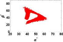
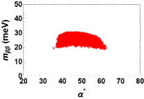
Figure 1: Correlation plots between (a) α𝛼\alpha and β𝛽\beta (b) α𝛼\alpha and mβ​βsubscriptπ‘šπ›½π›½m_{\beta\beta}. For the graphical analysis of Type-A1 texture, we set ΞΈ23=[39.6βˆ˜βˆ’β€‰51.8∘]subscriptπœƒ23delimited-[]superscript39.6superscript51.8\theta_{23}\,=\,[39.6^{\circ}\,-\,51.8^{\circ}] and δ𝛿\delta [108βˆ˜βˆ’β€‰404∘]delimited-[]superscript108superscript404[108^{\circ}\,-\,404^{\circ}].

We shall highlight one texture from each family as an example. We start with the Type-A family which contains eleven textures. To illustrate the formalism, we pluck the Type- A1 as an example. This texture shelters the following two correlations,

Re​[me​e]Redelimited-[]subscriptπ‘šπ‘’π‘’\displaystyle\text{Re}\,[m_{ee}] =\displaystyle= βˆ’Im​[me​μ],Imdelimited-[]subscriptπ‘šπ‘’πœ‡\displaystyle-\text{Im}\,[m_{e\mu}], (16)
Re​[me​μ]Redelimited-[]subscriptπ‘šπ‘’πœ‡\displaystyle\text{Re}\,[m_{e\mu}] =\displaystyle= βˆ’Im​[me​τ],Imdelimited-[]subscriptπ‘šπ‘’πœ\displaystyle-\text{Im}\,[m_{e\tau}], (17)

which are two transcendental equations, and we solve these two equations using Newton-Raphson method to predict α𝛼\alpha and β𝛽\beta. For this, we set initial values Ξ±0subscript𝛼0\alpha_{0} and Ξ²0subscript𝛽0\beta_{0} at 50∘superscript5050^{\circ} and 60∘superscript6060^{\circ} respectively. In addition, we fix m3subscriptπ‘š3m_{3} and δ𝛿\delta at 0.06​e​V0.06𝑒𝑉0.06\,eV and 270∘superscript270270^{\circ} respectively, whereas Δ​mi​j2Ξ”superscriptsubscriptπ‘šπ‘–π‘—2\Delta\,m_{ij}^{2} and ΞΈi​jsubscriptπœƒπ‘–π‘—\theta_{ij}’s are fixed at their best-fit values  [23]. This results in Ξ±=47.86βˆ˜π›Όsuperscript47.86\alpha=47.86^{\circ} and Ξ²=52.44βˆ˜π›½superscript52.44\beta=52.44^{\circ}. The details of the numerical results, for Type-A1 along with the other ten textures from the same family are elaborated in the Table 9. To see the predictions for α𝛼\alpha and β𝛽\beta in a more comprehensive way for Type-A1, we adopt a graphical analysis, for which, instead of choosing specific numerical values, we generate sufficient amount of random numbers for an specific input parameter which are consistent within the 3​σ3𝜎3\sigma bound as per Ref  [23]. We ensure that

6.82Γ—10βˆ’5​e​V2≀Δ​m212≀ 8.03Γ—10βˆ’5​e​V2,6.82superscript105𝑒superscript𝑉2Ξ”superscriptsubscriptπ‘š2128.03superscript105𝑒superscript𝑉2\displaystyle 6.82\times 10^{-5}\,eV^{2}\leq\Delta\,m_{21}^{2}\leq\,8.03\times 10^{-5}\,eV^{2}, (18)
2.428Γ—10βˆ’3​e​V2≀Δ​m312≀ 2.597Γ—10βˆ’3​e​V2,2.428superscript103𝑒superscript𝑉2Ξ”superscriptsubscriptπ‘š3122.597superscript103𝑒superscript𝑉2\displaystyle 2.428\times 10^{-3}\,eV^{2}\leq\Delta\,m_{31}^{2}\leq\,2.597\times 10^{-3}\,eV^{2}, (19)
31.31βˆ˜β‰€ΞΈ12≀35.74∘,superscript31.31subscriptπœƒ12superscript35.74\displaystyle 31.31^{\circ}\leq\theta_{12}\leq 35.74^{\circ}, (20)
8.19βˆ˜β‰€ΞΈ13≀ 8.89∘,superscript8.19subscriptπœƒ13superscript8.89\displaystyle 8.19^{\circ}\leq\theta_{13}\leq\,8.89^{\circ}, (21)
39.6βˆ˜β‰€ΞΈ23≀ 51.9∘.superscript39.6subscriptπœƒ23superscript51.9\displaystyle 39.6^{\circ}\leq\theta_{23}\leq\,51.9^{\circ}. (22)
108βˆ˜β‰€Ξ΄β‰€β€‰404∘.superscript108𝛿superscript404\displaystyle 108^{\circ}\leq\delta\leq\,404^{\circ}. (23)

We choose the other input parameter, 0.055​e​V≀m3≀0.06​e​V0.055𝑒𝑉subscriptπ‘š30.06𝑒𝑉0.055\,eV\leq m_{3}\leq 0.06\,\,eV and this assures, (m1+m2+m3≀0.12​e​V)subscriptπ‘š1subscriptπ‘š2subscriptπ‘š30.12𝑒𝑉(m_{1}\,+\,m_{2}\,+\,m_{3}\leq 0.12\,eV) [40]111We wish to state that for the graphical analysis shown in Figs. (1)-(6), we strictly adhere to the input ranges prescribed here. However, for Type-B1 and Type-Q1, the input δ𝛿\delta is not required and similarly, for Type-C1 and Type-R1, both δ𝛿\delta and ΞΈ23subscriptπœƒ23\theta_{23} are redundant.. Following this, we solve Eqs (16) and (17) and generate sufficient data points as predictions for α𝛼\alpha and β𝛽\beta which are illustrated graphically in Fig. 1). We see that the predictions of the two Majorana phases are constrained.

Similarly in Type-B category, we generate twelve textures. For example, Type-B1 texture underlines the following relations,

Im​[me​e]Imdelimited-[]subscriptπ‘šπ‘’π‘’\displaystyle\text{Im}\,[m_{ee}] =\displaystyle= βˆ’3​Re​[me​e],3Redelimited-[]subscriptπ‘šπ‘’π‘’\displaystyle-3\,\text{Re}\,[m_{ee}], (24)
Re​[me​μ]Redelimited-[]subscriptπ‘šπ‘’πœ‡\displaystyle\text{Re}\,[m_{e\mu}] =\displaystyle= βˆ’Im​[me​μ],Imdelimited-[]subscriptπ‘šπ‘’πœ‡\displaystyle-\text{Im}\,[m_{e\mu}], (25)
2​Re​[me​τ]2Redelimited-[]subscriptπ‘šπ‘’πœ\displaystyle 2\,\text{Re}\,[m_{e\tau}] =\displaystyle= βˆ’Im​[me​τ].Imdelimited-[]subscriptπ‘šπ‘’πœ\displaystyle-\text{Im}\,[m_{e\tau}]. (26)

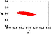
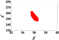
We shall exploit these three transcendental equations to predict δ𝛿\delta in addition to α𝛼\alpha and β𝛽\beta. With respect to a certain choice of the initial values Ξ±0subscript𝛼0\alpha_{0}, Ξ²0subscript𝛽0\beta_{0} and Ξ΄0subscript𝛿0\delta_{0}, the above three relations predict three physical parameters α𝛼\alpha, β𝛽\beta and δ𝛿\delta as 51.93∘superscript51.9351.93^{\circ}, 55.51∘superscript55.5155.51^{\circ} and 259.99∘superscript259.99259.99^{\circ} respectively. The detail of the required initial values of the said parameters along with the numerical results related to predictions for all textures under Type-B family are elaborated in Table 10. As before, to analyse graphically the credibility of Type-B1 texture, we solve the above three Eqs. (24)-(26) to generate sufficient random numbers for the parameters and obtain the correlation plots. From the plots, we identify the constrained bounds for the parameters α𝛼\alpha, β𝛽\beta, δ𝛿\delta and mβ​βsubscriptπ‘šπ›½π›½m_{\beta\beta} (see Fig. 2).

Refer to caption
Refer to caption
Refer to caption
Figure 2: Correlation plots between (a) α𝛼\alpha and β𝛽\beta (b) β𝛽\beta and δ𝛿\delta (c) δ𝛿\delta and mβ​βsubscriptπ‘šπ›½π›½m_{\beta\beta}. For the graphical analysis of Type-B1 texture, we set ΞΈ23=[39.6βˆ˜βˆ’β€‰51.8∘]subscriptπœƒ23delimited-[]superscript39.6superscript51.8\theta_{23}\,=\,[39.6^{\circ}\,-\,51.8^{\circ}].

The Type-C family carries five textures. Out of which, the Type-C1 texture is exemplified. It deals with the following four relations,

3​Im​[mμ​μ]3Imdelimited-[]subscriptπ‘šπœ‡πœ‡\displaystyle 3\,\text{Im}\,[m_{\mu\mu}] =\displaystyle= Im​[me​τ],Imdelimited-[]subscriptπ‘šπ‘’πœ\displaystyle\text{Im}\,[m_{e\tau}], (27)
Re​[me​μ]Redelimited-[]subscriptπ‘šπ‘’πœ‡\displaystyle\text{Re}\,[m_{e\mu}] =\displaystyle= βˆ’Re​[me​τ],Redelimited-[]subscriptπ‘šπ‘’πœ\displaystyle-\text{Re}\,[m_{e\tau}], (28)
Im​[me​τ]Imdelimited-[]subscriptπ‘šπ‘’πœ\displaystyle\text{Im}\,[m_{e\tau}] =\displaystyle= βˆ’Re​[me​e],Redelimited-[]subscriptπ‘šπ‘’π‘’\displaystyle-\text{Re}\,[m_{ee}], (29)
Im​[mτ​τ]Imdelimited-[]subscriptπ‘šπœπœ\displaystyle\text{Im}\,[m_{\tau\tau}] =\displaystyle= 2​Im​[mμ​τ],2Imdelimited-[]subscriptπ‘šπœ‡πœ\displaystyle 2\,\text{Im}\,[m_{\mu\tau}], (30)

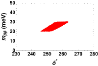
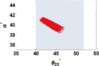
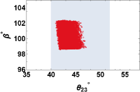
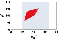
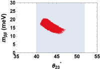
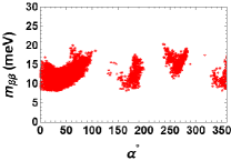
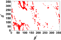
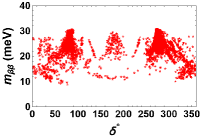
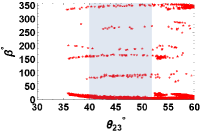
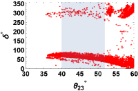
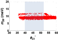
and hence, can predict four observables: α𝛼\alpha, β𝛽\beta, δ𝛿\delta and ΞΈ23subscriptπœƒ23\theta_{23}. We take proper choices of the initial values and Type-C1 predicts: α𝛼\alpha as 41.41∘superscript41.4141.41^{\circ} , β𝛽\beta as 100.3∘superscript100.3100.3^{\circ}, δ𝛿\delta as 99.81∘superscript99.8199.81^{\circ} and ΞΈ23subscriptπœƒ23\theta_{23} as 41.16∘superscript41.1641.16^{\circ}. The details of the input and predicted values of the Type-C textures can be found in Table 11. Following the same approach as before, we obtain the correlation plots and identify the constrained regions for the parameters α𝛼\alpha, β𝛽\beta, δ𝛿\delta, ΞΈ23subscriptπœƒ23\theta_{23} and mβ​βsubscriptπ‘šπ›½π›½m_{\beta\beta} (see Fig. 3).

Refer to caption
Refer to caption
Refer to caption
Refer to caption
Figure 3: Correlation plots between (a) ΞΈ23subscriptπœƒ23\theta_{23} and α𝛼\alpha (b) ΞΈ23subscriptπœƒ23\theta_{23} and β𝛽\beta (c) ΞΈ23subscriptπœƒ23\theta_{23} and δ𝛿\delta (d) ΞΈ23subscriptπœƒ23\theta_{23} and mβ​βsubscriptπ‘šπ›½π›½m_{\beta\beta}. The blue strip represent the 3​σ3𝜎3\sigma range of the observational parameter ΞΈ23subscriptπœƒ23\theta_{23}.

Similarly, we find twelve textures in Type-P family. To exemplify, we see that the Type-P1 texture deals with the following relations,

2​|me​e|2subscriptπ‘šπ‘’π‘’\displaystyle 2\,|m_{ee}| =\displaystyle= |mμ​μ|,subscriptπ‘šπœ‡πœ‡\displaystyle|m_{\mu\mu}|, (31)
|me​μ|subscriptπ‘šπ‘’πœ‡\displaystyle|m_{e\mu}| =\displaystyle= |me​τ|,subscriptπ‘šπ‘’πœ\displaystyle|m_{e\tau}|, (32)

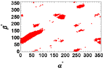
and predict the Majorana phases α𝛼\alpha and β𝛽\beta as 6.77∘superscript6.776.77^{\circ} and 80.77∘superscript80.7780.77^{\circ} respectively, with respect to certain initial choices Ξ±0subscript𝛼0\alpha_{0} and Ξ²0subscript𝛽0\beta_{0}. The details of the numerical inputs and predicted values of the parameters under Type-P textures are presented in the Table 12. To explore the possible regions of α𝛼\alpha, β𝛽\beta and mβ​βsubscriptπ‘šπ›½π›½m_{\beta\beta} for which Type-P1 texture is valid, we generate the correlation plot (see Fig. 4).
Refer to caption
Refer to caption
Figure 4: Correlation plots between (a) α𝛼\alpha and β𝛽\beta (b) α𝛼\alpha and mβ​βsubscriptπ‘šπ›½π›½m_{\beta\beta}. For the graphical analysis of Type-A1 texture, we set ΞΈ23=[39.6βˆ˜βˆ’β€‰51.8∘]subscriptπœƒ23delimited-[]superscript39.6superscript51.8\theta_{23}\,=\,[39.6^{\circ}\,-\,51.8^{\circ}] and δ𝛿\delta [108βˆ˜βˆ’β€‰404∘]delimited-[]superscript108superscript404[108^{\circ}\,-\,404^{\circ}].

We organize seven textures in Type-Q category. We put forward Type-Q1 as an example which shelters three relations as shown,

3​|me​e|3subscriptπ‘šπ‘’π‘’\displaystyle 3\,|m_{ee}| =\displaystyle= arg​[me​μ],argdelimited-[]subscriptπ‘šπ‘’πœ‡\displaystyle\text{arg}\,[m_{e\mu}], (33)
2​|me​μ|2subscriptπ‘šπ‘’πœ‡\displaystyle 2\,|m_{e\mu}| =\displaystyle= arg​[mτ​τ],argdelimited-[]subscriptπ‘šπœπœ\displaystyle\text{arg}\,[m_{\tau\tau}], (34)
|me​τ|subscriptπ‘šπ‘’πœ\displaystyle|m_{e\tau}| =\displaystyle= 2​arg​[mμ​μ],2argdelimited-[]subscriptπ‘šπœ‡πœ‡\displaystyle 2\,\text{arg}\,[m_{\mu\mu}], (35)

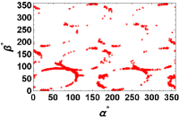
which are exploited to predict α𝛼\alpha, β𝛽\beta and δ𝛿\delta. With certain choices of initial values, we estimate α𝛼\alpha, β𝛽\beta and δ𝛿\delta as 92.57∘superscript92.5792.57^{\circ}, 26.88∘superscript26.8826.88^{\circ} and 165.01∘superscript165.01165.01^{\circ} respectively. The associated numerical inputs and results for all seven textures under Type-Q family are presented in Table 13. To visualise graphically, we generate the correlation plots and identify the constrained regions for the above said parameters (see Fig. 5).
Refer to caption
Refer to caption
Refer to caption
Figure 5: Correlation plots between (a) α𝛼\alpha and β𝛽\beta (b) β𝛽\beta and δ𝛿\delta (c) δ𝛿\delta and mβ​βsubscriptπ‘šπ›½π›½m_{\beta\beta}. For the graphical analysis of Type-B1 texture, we set ΞΈ23=[39.6βˆ˜βˆ’β€‰51.8∘]subscriptπœƒ23delimited-[]superscript39.6superscript51.8\theta_{23}\,=\,[39.6^{\circ}\,-\,51.8^{\circ}].

In fine, we work out six textures in Type-R category. For example, in Type-R1 texture, the following transcendental equations

3​|me​e|3subscriptπ‘šπ‘’π‘’\displaystyle 3\,|m_{ee}| =\displaystyle= arg​[mτ​τ],argdelimited-[]subscriptπ‘šπœπœ\displaystyle\text{arg}\,[m_{\tau\tau}], (36)
|me​μ|subscriptπ‘šπ‘’πœ‡\displaystyle|m_{e\mu}| =\displaystyle= 2​arg​[mτ​τ],2argdelimited-[]subscriptπ‘šπœπœ\displaystyle 2\,\text{arg}\,[m_{\tau\tau}], (37)
|me​τ|subscriptπ‘šπ‘’πœ\displaystyle|m_{e\tau}| =\displaystyle= 2​arg​[me​e],2argdelimited-[]subscriptπ‘šπ‘’π‘’\displaystyle 2\,\text{arg}[m_{ee}], (38)
|mμ​τ|subscriptπ‘šπœ‡πœ\displaystyle|m_{\mu\tau}| =\displaystyle= 3​arg​[me​e],3argdelimited-[]subscriptπ‘šπ‘’π‘’\displaystyle 3\,\text{arg}\,[m_{ee}], (39)

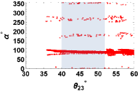
coexist and hence the texture may predict four observable parameters: α𝛼\alpha, β𝛽\beta, δ𝛿\delta and ΞΈ23subscriptπœƒ23\theta_{23} which are predicted as 98.64∘superscript98.6498.64^{\circ}, 18.69∘superscript18.6918.69^{\circ}, 40.59∘superscript40.5940.59^{\circ} and 40.78∘superscript40.7840.78^{\circ} respectively. These predictions are subjected to certain initial choices of the said parameters and are described in Table 14. The latter highlights the initial values as well as predictions related to all the textures of Type-Q family. We generate the corresponding correlation plots plots and identify the constrained bounds for the above mentioned parameters (see Fig. 6).
Refer to caption
Refer to caption
Refer to caption
Refer to caption
Figure 6: Correlation plots between (a) ΞΈ23subscriptπœƒ23\theta_{23} and α𝛼\alpha (b) ΞΈ23subscriptπœƒ23\theta_{23} and β𝛽\beta (c) ΞΈ23subscriptπœƒ23\theta_{23} and δ𝛿\delta (d) ΞΈ23subscriptπœƒ23\theta_{23} and mβ​βsubscriptπ‘šπ›½π›½m_{\beta\beta}. The blue strip represent the 3​σ3𝜎3\sigma range of the observational parameter ΞΈ23subscriptπœƒ23\theta_{23}.

Here, we emphasize that the predictions regarding the observational parameters with respect to relevant textures detailed in Tables (9)-(14) are sensitive to the initial values of the observational parameters. It is important to note that the numerical value associated with the prediction of a given texture is not unique; rather, there exist multiple viable solutions. For the Tables (9) to (14), we chose the inputs, namely Δ​m212Ξ”superscriptsubscriptπ‘š212\Delta m_{21}^{2}, Δ​m312Ξ”superscriptsubscriptπ‘š312\Delta m_{31}^{2}, ΞΈ12subscriptπœƒ12\theta_{12} and ΞΈ13subscriptπœƒ13\theta_{13} as the best-fit values  [23] with an exception of the Type-Q5 texture in Table. (13), where Δ​m312Ξ”superscriptsubscriptπ‘š312\Delta m_{31}^{2} is set to 2.53Γ—10βˆ’3​e​V22.53superscript103𝑒superscript𝑉22.53\times 10^{-3}\,eV^{2} (within 1​σ1𝜎1\sigma rangeΒ [23]). Furthermore, for all the above mentioned tables, we fix m3subscriptπ‘š3m_{3} at 0.06​e​V0.06𝑒𝑉0.06\,eV. For Tables (9) and (12), the Dirac CP phase δ𝛿\delta is fixed at 270∘superscript270270^{\circ}. Except for Tables  (11) and (14), the mixing angle ΞΈ23subscriptπœƒ23\theta_{23} is fixed at its best-fit valueΒ [23]. Following the predictions obtained from Tables (9)-(14), we predict the numerical values of the parameter mβ​βsubscriptπ‘šπ›½π›½m_{\beta\beta} corresponding to fifty-three proposed textures in Tables (15) and (16).

The Majorana phases are undetermined in the experiments. In principle, they can take any value between 0∘superscript00^{\circ} to 360∘superscript360360^{\circ}. However, in the Ref[43], it is shown that the Majorana CP phases can be chosen to lie within [0βˆ˜βˆ’180∘]delimited-[]superscript0superscript180[0^{\circ}-180^{\circ}] whereas the Dirac CP phase δ𝛿\delta can take any value within [0βˆ˜βˆ’360∘]delimited-[]superscript0superscript360[0^{\circ}-360^{\circ}]. We see that the prediction for β𝛽\beta from Type-Q5 texture contradicts with Ref[43]. In the present work, we attempt to constrain the values of the Majorana phases so that in future experiments they can be tested. We highlight that the neutrino mass matrix textures obtained in the present work are consistent with the data obtained from oscillation experiments. All the predicted values of δ𝛿\delta and ΞΈ23subscriptπœƒ23\theta_{23} under Type-B,C,Q,R textures lie within the 3​σ3𝜎3\sigma range of neutrino oscillation data. However, the Majorana phases are unobservable in the oscillation experiments. The viability of the proposed textures is subjected to the future experiments as discussed in section 1.

4 Symmetry Realization

All the neutrino mass matrix textures proposed in the present work are obtained from phenomenological ground by following the bottom up approach. Though these textures are model independent, it is expected that they can be derived from the first principle. To make the discussion more fruitful, we try to realize the underlying possible symmetry groups working behind one specific texture from each category.

4.1 Type-A3

The Type-A3 texture deals with two constrained relations,

Re​[mτ​τ]Redelimited-[]subscriptπ‘šπœπœ\displaystyle\text{Re}\,[m_{\tau\tau}] =\displaystyle= βˆ’2​Re​[me​τ],2Redelimited-[]subscriptπ‘šπ‘’πœ\displaystyle-2\,\text{Re}\,[m_{e\tau}], (40)
Im​[me​τ]Imdelimited-[]subscriptπ‘šπ‘’πœ\displaystyle\text{Im}\,[m_{e\tau}] =\displaystyle= Im​[mμ​τ].Imdelimited-[]subscriptπ‘šπœ‡πœ\displaystyle\text{Im}\,[m_{\mu\tau}]. (41)

To derive this particular texture, we extend the SM by introducing two additional S​U​(2)Lπ‘†π‘ˆsubscript2𝐿SU(2)_{L} doublet, three S​U​(2)Lπ‘†π‘ˆsubscript2𝐿SU(2)_{L} triplet Higgs fields and three S​U​(2)Lπ‘†π‘ˆsubscript2𝐿SU(2)_{L} singlet fields. The right-handed neutrino field transforms as triplet under A4subscript𝐴4A_{4}. We consider that the right-handed neutrino field and the additional S​U​(2)Lπ‘†π‘ˆsubscript2𝐿SU(2)_{L} triplet Higgs fields contribute to the effective neutrino mass matrix via Type-I and Type-II mechanisms respectively. The additional symmetry Z2subscript𝑍2Z_{2} is incorporated along with A4subscript𝐴4A_{4} in order to restrict the unwanted terms that are allowed by the latter. The transformation of all the field contents of our proposed model with their respective assignments under the group S​U​(2)LΓ—A4Γ—Z2π‘†π‘ˆsubscript2𝐿subscript𝐴4subscript𝑍2SU(2)_{L}\times A_{4}\times Z_{2} are summarised in Table 17.

The S​U​(2)LΓ—A4Γ—Z2π‘†π‘ˆsubscript2𝐿subscript𝐴4subscript𝑍2SU(2)_{L}\times A_{4}\times Z_{2} invariant Yukawa Lagrangian can be constructed in the following manner,

βˆ’β„’Ysubscriptβ„’π‘Œ\displaystyle-\mathcal{L}_{Y} =\displaystyle= ye​(DΒ―lL​Φ)1​eR1+yμ​(DΒ―lL​Φ)1′​μR1β€²β€²+yτ​(DΒ―lL​Φ)1′′​τR1β€²+subscript𝑦𝑒subscriptsubscript¯𝐷subscript𝑙𝐿Φ1subscript𝑒subscript𝑅1subscriptπ‘¦πœ‡subscriptsubscript¯𝐷subscript𝑙𝐿Φsuperscript1β€²subscriptπœ‡subscript𝑅superscript1β€²β€²limit-fromsubscriptπ‘¦πœsubscriptsubscript¯𝐷subscript𝑙𝐿Φsuperscript1β€²β€²subscript𝜏subscript𝑅superscript1β€²\displaystyle y_{e}(\bar{D}_{l_{L}}\Phi)_{1}\,e_{R_{1}}+y_{\mu}(\bar{D}_{l_{L}}\Phi)_{1^{\prime}}\,\mu_{R_{1^{\prime\prime}}}+y_{\tau}(\bar{D}_{l_{L}}\Phi)_{1^{\prime\prime}}\,\tau_{R_{1^{\prime}}}+ (42)
yD​{(DΒ―lL​Φ~)3S​νR+(DΒ―lL​Φ~)3A​νR}+12​yR1​(Ξ½Β―R​νRc)1​η+subscript𝑦𝐷subscriptsubscript¯𝐷subscript𝑙𝐿~Ξ¦subscript3𝑆subscriptπœˆπ‘…subscriptsubscript¯𝐷subscript𝑙𝐿~Ξ¦subscript3𝐴subscriptπœˆπ‘…limit-from12subscript𝑦subscript𝑅1subscriptsubscriptΒ―πœˆπ‘…subscriptsuperscriptπœˆπ‘π‘…1πœ‚\displaystyle y_{D}\{(\bar{D}_{l_{L}}\tilde{\Phi})_{3_{S}}\,\nu_{R}+(\bar{D}_{l_{L}}\tilde{\Phi})_{3_{A}}\,\nu_{R}\}+\frac{1}{2}\,y_{R_{1}}(\bar{\nu}_{R}\,\nu^{c}_{R})_{1}\,\eta\,+
12​yR2​(Ξ½Β―R​νRc)3​κ+12​yR3​(Ξ½Β―R​νRc)3​ξ+yT​(DΒ―lL​DlLc)3​Δ12subscript𝑦subscript𝑅2subscriptsubscriptΒ―πœˆπ‘…subscriptsuperscriptπœˆπ‘π‘…3πœ…12subscript𝑦subscript𝑅3subscriptsubscriptΒ―πœˆπ‘…subscriptsuperscriptπœˆπ‘π‘…3πœ‰subscript𝑦𝑇subscriptsubscript¯𝐷subscript𝑙𝐿superscriptsubscript𝐷subscript𝑙𝐿𝑐3Ξ”\displaystyle\frac{1}{2}\,y_{R_{2}}(\bar{\nu}_{R}\,\nu^{c}_{R})_{3}\,\kappa+\frac{1}{2}\,y_{R_{3}}(\bar{\nu}_{R}\,\nu^{c}_{R})_{3}\,\xi\,+\,y_{T}(\bar{D}_{l_{L}}\,D_{l_{L}}^{c})_{3}\,\Delta\,
+h.c.,formulae-sequenceβ„Žπ‘\displaystyle+\,h.c.,

where, Ξ¦~=i​τ2β€‹Ξ¦βˆ—~Φ𝑖subscript𝜏2superscriptΞ¦\tilde{\Phi}=i\tau_{2}\Phi^{*}. The products rules under A4subscript𝐴4A_{4} group can be found in B. It is important to mention that we choose a specific VEV alignment (Ξ¦i)subscriptΦ𝑖(\Phi_{i}) as ⟨Φ⟩0=v​(1,Ο‰,Ο‰2)Tsubscriptdelimited-⟨⟩Φ0𝑣superscript1πœ”superscriptπœ”2𝑇\langle\Phi\rangle_{0}\,=\,v\,(1,\omega,\omega^{2})^{T} (a similar choice is mentioned in ref Β [44]), where, Ο‰=e2​π​i/3πœ”superscript𝑒2πœ‹π‘–3\omega=e^{2\pi i/3} and Ο‰2=eβˆ’2​π​i/3superscriptπœ”2superscript𝑒2πœ‹π‘–3\omega^{2}=e^{-2\pi i/3}. In the symmetry basis, such a choice of the VEVs lead us to the charged lepton mass matrix of the following form,

ML=v​[yeyΞΌyΟ„ye​ωyΞΌyτ​ω2ye​ω2yΞΌyτ​ω].subscript𝑀𝐿𝑣matrixsubscript𝑦𝑒subscriptπ‘¦πœ‡subscriptπ‘¦πœsubscriptπ‘¦π‘’πœ”subscriptπ‘¦πœ‡subscriptπ‘¦πœsuperscriptπœ”2subscript𝑦𝑒superscriptπœ”2subscriptπ‘¦πœ‡subscriptπ‘¦πœπœ”M_{L}=v\begin{bmatrix}y_{e}&y_{\mu}&y_{\tau}\\ y_{e}\omega&y_{\mu}&y_{\tau}\omega^{2}\\ y_{e}\omega^{2}&y_{\mu}&y_{\tau}\omega\\ \end{bmatrix}. (43)

On the other hand, the Dirac neutrino mass matrix is obtained as shown below,

MD=2​yD​v​[00ωω200010].subscript𝑀𝐷2subscript𝑦𝐷𝑣matrix00πœ”superscriptπœ”200010M_{D}=2\,y_{D}\,v\begin{bmatrix}0&0&\omega\\ \omega^{2}&0&0\\ 0&1&0\\ \end{bmatrix}. (44)

We assume that the fields ΞΊπœ…\kappa and ΞΎπœ‰\xi attain the VEV alignments vκ​(0,0,1)Tsubscriptπ‘£πœ…superscript001𝑇v_{\kappa}(0,0,1)^{T} and vξ​(1,0,0)Tsubscriptπ‘£πœ‰superscript100𝑇v_{\xi}(1,0,0)^{T} while ⟨η⟩=vΞ·delimited-βŸ¨βŸ©πœ‚subscriptπ‘£πœ‚\langle\eta\rangle=v_{\eta} such that the right-handed neutrino mass matrix takes the following form,

MR=[pq0qpr0rp],subscript𝑀𝑅matrixπ‘π‘ž0π‘žπ‘π‘Ÿ0π‘Ÿπ‘M_{R}=\begin{bmatrix}p&q&0\\ q&p&r\\ 0&r&p\\ \end{bmatrix}, (45)

where, p=yR1​vη𝑝subscript𝑦subscript𝑅1subscriptπ‘£πœ‚p=y_{R_{1}}v_{\eta}, q=yR2​vΞΊπ‘žsubscript𝑦subscript𝑅2subscriptπ‘£πœ…q=y_{R_{2}}v_{\kappa}, r=yR3​vΞΎπ‘Ÿsubscript𝑦subscript𝑅3subscriptπ‘£πœ‰r=y_{R_{3}}v_{\xi}. For the sake of simplicity, we take the following choices: q=2​pπ‘ž2𝑝q=2p and r=3​pπ‘Ÿ3𝑝r=3p.

After the redefinition of some parameters, we obtain the neutrino mass matrix from Type-I seesaw mechanism in the following way,

MT1subscript𝑀subscript𝑇1\displaystyle M_{T_{1}} =\displaystyle= βˆ’MD​MRβˆ’1​MDTsubscript𝑀𝐷subscriptsuperscript𝑀1𝑅subscriptsuperscript𝑀𝑇𝐷\displaystyle-M_{D}M^{-1}_{R}M^{T}_{D} (46)
=\displaystyle= [βˆ’a​ω22​aβˆ’a​ω2​aβˆ’83​aβ€‹Ο‰βˆ’23​a​ω2βˆ’aβ€‹Ο‰βˆ’23​a​ω2a3]matrixπ‘Žsuperscriptπœ”22π‘Žπ‘Žπœ”2π‘Ž83π‘Žπœ”23π‘Žsuperscriptπœ”2π‘Žπœ”23π‘Žsuperscriptπœ”2π‘Ž3\displaystyle\begin{bmatrix}-a\omega^{2}&2a&-a\omega\\ 2a&\frac{-8}{3}a\omega&\frac{-2}{3}a\omega^{2}\\ -a\omega&\frac{-2}{3}a\omega^{2}&\frac{a}{3}\\ \end{bmatrix}

Assuming that the Higgs triplet takes VEVs along the direction βŸ¨Ξ”βŸ©0=vΔ​(0,1,1)Tsubscriptdelimited-βŸ¨βŸ©Ξ”0subscript𝑣Δsuperscript011𝑇\langle\Delta\rangle_{0}=v_{\Delta}(0,1,1)^{T}, the Type-II contribution to the effective neutrino mass matrix takes the following form,

MT2=d​[011100100],where,​d=yT​vΞ”formulae-sequencesubscript𝑀subscript𝑇2𝑑matrix011100100where,𝑑subscript𝑦𝑇subscript𝑣ΔM_{T_{2}}=d\begin{bmatrix}0&1&1\\ 1&0&0\\ 1&0&0\\ \end{bmatrix},\,\,\,\,\,\,\,\,\,\,\,\,\,\,\,\,\,\,\,\,\,\,\text{where,}\,\,\,\,\,d=y_{T}v_{\Delta} (47)

After taking the contributions from Type-I and Type-II seesaw, the effective neutrino mass matrix can be written as,

MΞ½subscriptπ‘€πœˆ\displaystyle M_{\nu} =MT1+MT2absentsubscript𝑀subscript𝑇1subscript𝑀subscript𝑇2\displaystyle=M_{T_{1}}+M_{T_{2}} =[βˆ’a​ω22​a+dβˆ’a​w+d2​a+dβˆ’83​aβ€‹Ο‰βˆ’23​a​ω2βˆ’a​ω+dβˆ’23​a​ω2a3].absentmatrixπ‘Žsuperscriptπœ”22π‘Žπ‘‘π‘Žπ‘€π‘‘2π‘Žπ‘‘83π‘Žπœ”23π‘Žsuperscriptπœ”2π‘Žπœ”π‘‘23π‘Žsuperscriptπœ”2π‘Ž3\displaystyle=\begin{bmatrix}-a\omega^{2}&2a+d&-aw+d\\ 2a+d&\frac{-8}{3}a\omega&\frac{-2}{3}a\omega^{2}\\ -a\omega+d&\frac{-2}{3}a\omega^{2}&\frac{a}{3}\\ \end{bmatrix}. (48)

To move from symmetry basis to flavour basis, we need to diagonalise Mlsubscript𝑀𝑙M_{l} in the following way,

Mld​i​a​g=Ul†​Ml​Ur,subscriptsuperscriptπ‘€π‘‘π‘–π‘Žπ‘”π‘™superscriptsubscriptπ‘ˆπ‘™β€ subscript𝑀𝑙subscriptπ‘ˆπ‘ŸM^{diag}_{l}=U_{l}^{\dagger}M_{l}U_{r}, (49)

where,

Ul=13​[1111Ο‰2Ο‰1ωω2]​and​Ur=[001100010].subscriptπ‘ˆπ‘™13matrix1111superscriptπœ”2πœ”1πœ”superscriptπœ”2andsubscriptπ‘ˆπ‘Ÿmatrix001100010U_{l}=\frac{1}{\sqrt{3}}\begin{bmatrix}1&1&1\\ 1&\omega^{2}&\omega\\ 1&\omega&\omega^{2}\\ \end{bmatrix}\,\,\,\text{and}\,\,\,U_{r}=\begin{bmatrix}0&0&1\\ 1&0&0\\ 0&1&0\\ \end{bmatrix}. (50)

In the flavour basis, the effective neutrino mass matrix is also perturbed by the charged lepton correction (UlL†​MΞ½s​UlLβˆ—subscriptsuperscriptπ‘ˆβ€ subscript𝑙𝐿subscript𝑀subscriptπœˆπ‘ subscriptsuperscriptπ‘ˆsubscript𝑙𝐿U^{\dagger}_{l_{L}}M_{\nu_{s}}U^{*}_{l_{L}}) which is expressed in the following manner,

MΞ½f=[A+i​BC+i​D𝐄+i​𝐅C+i​DG+i​HJ+i​𝐅E+i​FJ+i​Fβˆ’πŸβ€‹π„βˆ’2​i​F].subscriptsuperscriptπ‘€π‘“πœˆmatrix𝐴𝑖𝐡𝐢𝑖𝐷𝐄𝑖𝐅𝐢𝑖𝐷𝐺𝑖𝐻𝐽𝑖𝐅𝐸𝑖𝐹𝐽𝑖𝐹2𝐄2𝑖𝐹M^{f}_{\nu}=\begin{bmatrix}A+iB&C+iD&\mathbf{E}+i\mathbf{F}\\ C+iD&G+iH&J+i\mathbf{F}\\ E+iF&J+iF&-\mathbf{2E}-2iF\\ \end{bmatrix}. (51)

From the neutrino mass matrix appearing in Eq. 51, we see that the mass matrix elements (MΞ½f)e​τsubscriptsubscriptsuperscriptπ‘€π‘“πœˆπ‘’πœ(M^{f}_{\nu})_{e\tau}, (MΞ½f)μ​τsubscriptsubscriptsuperscriptπ‘€π‘“πœˆπœ‡πœ(M^{f}_{\nu})_{\mu\tau} and (MΞ½f)τ​τsubscriptsubscriptsuperscriptπ‘€π‘“πœˆπœπœ(M^{f}_{\nu})_{\tau\tau} exhibit the relations prescribed in Eqs. (40) and (41). Thus, the above mass matrix, MΞ½fsuperscriptsubscriptπ‘€πœˆπ‘“M_{\nu}^{f} resembles Type-A3 texture.

4.2 Type-B8

The Type-B8 texture shelters three constrained relations:

Re​[me​μ]Redelimited-[]subscriptπ‘šπ‘’πœ‡\displaystyle\text{Re}\,[m_{e\mu}] =\displaystyle= Im​[me​τ],Imdelimited-[]subscriptπ‘šπ‘’πœ\displaystyle\text{Im}\,[m_{e\tau}], (52)
Re​[me​e]Redelimited-[]subscriptπ‘šπ‘’π‘’\displaystyle\text{Re}\,[m_{ee}] =\displaystyle= βˆ’Im​[mμ​τ],Imdelimited-[]subscriptπ‘šπœ‡πœ\displaystyle-\text{Im}\,[m_{\mu\tau}], (53)
Im​[mμ​μ]Imdelimited-[]subscriptπ‘šπœ‡πœ‡\displaystyle\text{Im}\,[m_{\mu\mu}] =\displaystyle= βˆ’Im​[mτ​τ].Imdelimited-[]subscriptπ‘šπœπœ\displaystyle-\text{Im}\,[m_{\tau\tau}]. (54)

To derive the Type-B8 texture, we extend the field content of the SM by introducing right-handed neutrinos (Ξ½eR,Ξ½ΞΌR,Ξ½Ο„R)subscript𝜈subscript𝑒𝑅subscript𝜈subscriptπœ‡π‘…subscript𝜈subscriptπœπ‘…(\nu_{e_{R}},\nu_{\mu_{R}},\nu_{\tau_{R}}), two scalar singlets (ΞΊπœ…\kappa and Ο‚πœ\varsigma) and a scalar triplets (ΔΔ\Delta). We summarise the transformation properties of the field content associated with Δ​(27)Ξ”27\Delta\,(27) symmetry in Table 19. We construct the S​U​(2)L×Δ​(27)π‘†π‘ˆsubscript2𝐿Δ27SU(2)_{L}\times\Delta\,(27) invariant Lagrangian in the following way,

βˆ’β„’Ysubscriptβ„’π‘Œ\displaystyle-\mathcal{L}_{Y} =\displaystyle= ye​(DΒ―lL​H)100​eR100+yμ​(DΒ―lL​H)120​μR110+yτ​(DΒ―lL​H)110​τR120+subscript𝑦𝑒subscriptsubscript¯𝐷subscript𝑙𝐿𝐻subscript100subscript𝑒subscript𝑅subscript100subscriptπ‘¦πœ‡subscriptsubscript¯𝐷subscript𝑙𝐿𝐻subscript120subscriptπœ‡subscript𝑅subscript110limit-fromsubscriptπ‘¦πœsubscriptsubscript¯𝐷subscript𝑙𝐿𝐻subscript110subscript𝜏subscript𝑅subscript120\displaystyle y_{e}(\bar{D}_{l_{L}}H)_{1_{00}}\,e_{R_{1_{00}}}+y_{\mu}(\bar{D}_{l_{L}}H)_{{1_{20}}}\,\mu_{R_{1_{10}}}+\,y_{\tau}\,(\bar{D}_{l_{L}}H)_{{1_{10}}}\tau_{R_{1_{20}}}+ (55)
y1​(DΒ―lL​H~)100​νeR100+y2​(DΒ―lL​H~)110​νμR120+y3​(DΒ―lL​H~)120​ντR110subscript𝑦1subscriptsubscript¯𝐷subscript𝑙𝐿~𝐻subscript100subscript𝜈subscript𝑒subscript𝑅subscript100subscript𝑦2subscriptsubscript¯𝐷subscript𝑙𝐿~𝐻subscript110subscript𝜈subscriptπœ‡subscript𝑅subscript120subscript𝑦3subscriptsubscript¯𝐷subscript𝑙𝐿~𝐻subscript120subscript𝜈subscript𝜏subscript𝑅subscript110\displaystyle y_{1}\,(\bar{D}_{l_{L}}\tilde{H})_{{1_{00}}}\,\nu_{e_{R_{1_{00}}}}+y_{2}(\bar{D}_{l_{L}}\,\tilde{H})_{1_{10}}\nu_{\mu_{R_{1_{20}}}}+y_{3}(\bar{D}_{l_{L}}\tilde{H})_{1_{20}}\,\nu_{\tau_{R_{1_{10}}}}\,
+12​yR1​(Ξ½Β―Ο„R​ντRc)120​κ110+12​yR2​[(Ξ½Β―eR​νμRc)+(Ξ½Β―ΞΌR​νeRc)]120​κ11012subscript𝑦subscript𝑅1subscriptsubscript¯𝜈subscriptπœπ‘…subscriptsuperscriptπœˆπ‘subscriptπœπ‘…subscript120subscriptπœ…subscript11012subscript𝑦subscript𝑅2subscriptdelimited-[]subscript¯𝜈subscript𝑒𝑅subscriptsuperscriptπœˆπ‘subscriptπœ‡π‘…subscript¯𝜈subscriptπœ‡π‘…subscriptsuperscriptπœˆπ‘subscript𝑒𝑅subscript120subscriptπœ…subscript110\displaystyle+\frac{1}{2}\,y_{R_{1}}\,(\bar{\nu}_{\tau_{R}}\,\nu^{c}_{\tau_{R}})_{1_{20}}\,\kappa_{1_{10}}+\frac{1}{2}\,y_{R_{2}}\,[(\bar{\nu}_{e_{R}}\,\nu^{c}_{\mu_{R}})\,+(\bar{\nu}_{\mu_{R}}\,\nu^{c}_{e_{R}})]_{1_{20}}\,{\kappa}_{1_{10}}
+yT2​DΒ―lL3​(DlLc​Δ)3s1βˆ—+h.c.formulae-sequencesubscript𝑦subscript𝑇2subscript¯𝐷subscript𝑙subscript𝐿3subscriptsuperscriptsubscript𝐷subscript𝑙𝐿𝑐Δsubscriptsuperscript3subscript𝑠1β„Žπ‘\displaystyle+\,y_{T_{2}}\,\bar{D}_{l_{L_{3}}}\,(D_{l_{L}}^{c}\,{\Delta})_{3^{*}_{s_{1}}}+\,h.c.

The product rules under Δ​(27)Ξ”27\Delta\,(27) are given in C. We choose the complex vacuum alignment ⟨H⟩∘=vH​(w,1,1)Tsubscriptdelimited-⟨⟩𝐻subscript𝑣𝐻superscript𝑀11𝑇\langle H\rangle_{\circ}=v_{H}\,(w,1,1)^{T} as per ref [45] and obtain the charged lepton mass matrix as shown below,

Ml=vϕ​[Ο‰2​yeΟ‰2​yΞΌΟ‰2​yτω2​yeyμω​yτω​yeyΞΌΟ‰2​yΟ„],subscript𝑀𝑙subscript𝑣italic-Ο•matrixsuperscriptπœ”2subscript𝑦𝑒superscriptπœ”2subscriptπ‘¦πœ‡superscriptπœ”2subscriptπ‘¦πœsuperscriptπœ”2subscript𝑦𝑒subscriptπ‘¦πœ‡πœ”subscriptπ‘¦πœπœ”subscript𝑦𝑒subscriptπ‘¦πœ‡superscriptπœ”2subscriptπ‘¦πœM_{l}=v_{\phi}\begin{bmatrix}\omega^{2}\,y_{e}&\omega^{2}\,y_{\mu}&\omega^{2}\,y_{\tau}\\ \omega^{2}y_{e}&\,y_{\mu}&\omega\,y_{\tau}\\ \omega y_{e}&\,y_{\mu}&\omega^{2}\,y_{\tau}\\ \end{bmatrix}, (56)

where, Ο‰=ei​ 2​π/3πœ”superscript𝑒𝑖2πœ‹3\omega=e^{i\,2\pi/3}, Ο‰2=Ο‰βˆ—superscriptπœ”2superscriptπœ”\omega^{2}=\omega^{*}.

We diagonalise Mlsubscript𝑀𝑙M_{l} as Mld​i​a​g=UlL†​Ml​UlRsubscriptsuperscriptπ‘€π‘‘π‘–π‘Žπ‘”π‘™subscriptsuperscriptπ‘ˆβ€ subscript𝑙𝐿subscript𝑀𝑙subscriptπ‘ˆsubscript𝑙𝑅M^{diag}_{l}=\,U^{\dagger}_{l_{L}}M_{l}U_{l_{R}}, where, Mld​i​a​g=3​vH​d​i​a​g​(ye,yΞΌ,yΟ„)subscriptsuperscriptπ‘€π‘‘π‘–π‘Žπ‘”π‘™3subscriptπ‘£π»π‘‘π‘–π‘Žπ‘”subscript𝑦𝑒subscriptπ‘¦πœ‡subscriptπ‘¦πœM^{diag}_{l}=\,\sqrt{3}\,v_{H}\,diag\,(y_{e},\,y_{\mu},\,y_{\tau}). The UlLsubscriptπ‘ˆsubscript𝑙𝐿U_{l_{L}} and UlRsubscriptπ‘ˆsubscript𝑙𝑅U_{l_{R}} can be expressed in the following way,

UlLsubscriptπ‘ˆsubscript𝑙𝐿\displaystyle U_{l_{L}} =\displaystyle= 13​[Ο‰2​ei​΢eiβ€‹ΟˆΟ‰β€‹ei​φei​΢ω2​eiβ€‹ΟˆΟ‰β€‹ei​φei​΢eiβ€‹Οˆei​φ],13matrixsuperscriptπœ”2superscriptπ‘’π‘–πœsuperscriptπ‘’π‘–πœ“πœ”superscriptπ‘’π‘–πœ‘superscriptπ‘’π‘–πœsuperscriptπœ”2superscriptπ‘’π‘–πœ“πœ”superscriptπ‘’π‘–πœ‘superscriptπ‘’π‘–πœsuperscriptπ‘’π‘–πœ“superscriptπ‘’π‘–πœ‘\displaystyle\frac{1}{\sqrt{3}}\begin{bmatrix}\omega^{2}\,e^{i\zeta}&e^{i\psi}&\omega\,e^{i\varphi}\\ e^{i\zeta}&\omega^{2}\,e^{i\psi}&\omega\,e^{i\varphi}\\ e^{i\zeta}&e^{i\psi}&e^{i\varphi}\\ \end{bmatrix}, (57)
UlRsubscriptπ‘ˆsubscript𝑙𝑅\displaystyle U_{l_{R}} =\displaystyle= d​i​a​g​(ei​΢,Ο‰iβ€‹Οˆ,Ο‰2​ei​φ).π‘‘π‘–π‘Žπ‘”superscriptπ‘’π‘–πœsuperscriptπœ”π‘–πœ“superscriptπœ”2superscriptπ‘’π‘–πœ‘\displaystyle diag(e^{i\zeta},\,\omega\,^{i\psi},\,\omega^{2}\,e^{i\varphi}). (58)

It is to be noted that the choices of eigenvectors are not unique and we include the arbitrary phases (ΞΆ,ψ,Ο†πœπœ“πœ‘\zeta,\psi,\varphi) in UlLsubscriptπ‘ˆsubscript𝑙𝐿U_{l_{L}} and UlRsubscriptπ‘ˆsubscript𝑙𝑅U_{l_{R}}. It has many advantages which are highlighted in ref [46]. To experience the Type-B8 texture, we set ΞΆ=Ο€2πœπœ‹2\zeta=\frac{\pi}{2}, ψ=Ο€πœ“πœ‹\psi=\pi and Ο†=Ο€2πœ‘πœ‹2\varphi=\frac{\pi}{2}.

Under the choice of vacuum alignment ⟨H⟩∘=vH​(w,1,1)Tsubscriptdelimited-⟨⟩𝐻subscript𝑣𝐻superscript𝑀11𝑇\langle H\rangle_{\circ}=v_{H}\,(w,1,1)^{T} and ⟨κ⟩∘=vΞΊsubscriptdelimited-βŸ¨βŸ©πœ…subscriptπ‘£πœ…\langle\kappa\rangle_{\circ}=v_{\kappa}, the Dirac neutrino mass matrix (MDsubscript𝑀𝐷M_{D}) and right handed neutrino mass matrix (MRsubscript𝑀𝑅M_{R}) takes the following form,

MDsubscript𝑀𝐷\displaystyle M_{D} =\displaystyle= [x​ωy​ωz​ωxΟ‰2​yω​zxω​yΟ‰2​z],matrixπ‘₯πœ”π‘¦πœ”π‘§πœ”π‘₯superscriptπœ”2π‘¦πœ”π‘§π‘₯πœ”π‘¦superscriptπœ”2𝑧\displaystyle\begin{bmatrix}x\,\omega&y\,\omega&z\,\omega\\ x&\omega^{2}\,y&\omega\,z\\ x&\omega\,y&\omega^{2}\,z\\ \end{bmatrix}, (59)
MRsubscript𝑀𝑅\displaystyle M_{R} =\displaystyle= [0q0q0000p],matrix0π‘ž0π‘ž0000𝑝\displaystyle\begin{bmatrix}0&q&0\\ q&0&0\\ 0&0&p\\ \end{bmatrix}, (60)

where, x=y1​vHπ‘₯subscript𝑦1subscript𝑣𝐻x=y_{1}\,v_{H}, y=y2​vH𝑦subscript𝑦2subscript𝑣𝐻y=y_{2}\,v_{H}, z=y3​vH𝑧subscript𝑦3subscript𝑣𝐻z=y_{3}\,v_{H}, p=YR1​vκ𝑝subscriptπ‘Œsubscript𝑅1subscriptπ‘£πœ…p=Y_{R_{1}}\,v_{\kappa} and q=YR2​vΞΊπ‘žsubscriptπ‘Œsubscript𝑅2subscriptπ‘£πœ…q=Y_{R_{2}}\,v_{\kappa}.

The Type-I seesaw contributes as MT1=βˆ’MD​MRβˆ’1​MDTsubscript𝑀subscript𝑇1subscript𝑀𝐷subscriptsuperscript𝑀1𝑅subscriptsuperscript𝑀𝑇𝐷M_{T_{1}}=\,-\,M_{D}M^{-1}_{R}M^{T}_{D}. The choices of vacuum alignments βŸ¨Ξ”βŸ©βˆ˜=vΔ​(1,1,1)Tsubscriptdelimited-βŸ¨βŸ©Ξ”subscript𝑣Δsuperscript111𝑇\langle\Delta\rangle_{\circ}=v_{\Delta}(1,1,1)^{T} and βŸ¨Ο‡βŸ©βˆ˜=vΟ‡subscriptdelimited-βŸ¨βŸ©πœ’subscriptπ‘£πœ’\langle\chi\rangle_{\circ}=v_{\chi} for the ΔΔ\Delta Higgs and scalar field Ο‡πœ’\chi give rise to the Type-II contribution as shown below,

MT2=[r000r000r],subscript𝑀subscript𝑇2matrixπ‘Ÿ000π‘Ÿ000π‘ŸM_{T_{2}}=\begin{bmatrix}r&0&0\\ 0&r&0\\ 0&0&r\\ \end{bmatrix}, (61)

where, r=yT2​vΞ”π‘Ÿsubscript𝑦subscript𝑇2subscript𝑣Δr=y_{T_{2}}\,v_{\Delta}. In symmetry basis, we construct the neutrino mass matrix as MΞ½s=MT1+MT2subscript𝑀subscriptπœˆπ‘ subscript𝑀subscript𝑇1subscript𝑀subscript𝑇2M_{\nu_{s}}=M_{T_{1}}+M_{T_{2}}. In flavour basis, after taking the contribution from UlLsubscriptπ‘ˆsubscript𝑙𝐿U_{l_{L}}, the neutrino mass matrix takes the following form,

MΞ½f=[A+i​BC+i​DF+i​CC+i​DG+i​HJβˆ’i​AF+i​CJβˆ’i​Aβˆ’Gβˆ’i​H].subscriptsuperscriptπ‘€π‘“πœˆmatrixA𝑖𝐡C𝑖𝐷𝐹𝑖C𝐢𝑖𝐷𝐺𝑖H𝐽𝑖A𝐹𝑖𝐢𝐽𝑖𝐴𝐺𝑖HM^{f}_{\nu}=\begin{bmatrix}\textbf{A}+iB&\textbf{C}+iD&F+i\textbf{C}\\ C+iD&G+i\textbf{H}&J-i\textbf{A}\\ F+iC&J-iA&-G-i\textbf{H}\\ \end{bmatrix}. (62)

4.3 Type-C2

The Type-C2 texture shelters three constrained relations:

Re​[me​e]Redelimited-[]subscriptπ‘šπ‘’π‘’\displaystyle\text{Re}\,[m_{ee}] =\displaystyle= Re​[mμ​τ]Redelimited-[]subscriptπ‘šπœ‡πœ\displaystyle\text{Re}\,[m_{\mu\tau}] (63)
Re​[me​μ]Redelimited-[]subscriptπ‘šπ‘’πœ‡\displaystyle\text{Re}\,[m_{e\mu}] =\displaystyle= βˆ’Re​[me​τ]Redelimited-[]subscriptπ‘šπ‘’πœ\displaystyle-\text{Re}\,[m_{e\tau}] (64)
Im​[mμ​μ]Imdelimited-[]subscriptπ‘šπœ‡πœ‡\displaystyle\text{Im}\,[m_{\mu\mu}] =\displaystyle= Im​[mτ​τ]Imdelimited-[]subscriptπ‘šπœπœ\displaystyle\text{Im}\,[m_{\tau\tau}] (65)
Im​[mμ​μ]Imdelimited-[]subscriptπ‘šπœ‡πœ‡\displaystyle\text{Im}\,[m_{\mu\mu}] =\displaystyle= βˆ’Im​[mμ​τ]Imdelimited-[]subscriptπ‘šπœ‡πœ\displaystyle-\text{Im}\,[m_{\mu\tau}] (66)

We try to derive the Type-C2 texture from the same Lagrangian appearing in Eq. 55 with a modification in the Type-II contribution part. In this regard we add a scalar singlet Ο‡110subscriptπœ’subscript110\chi_{1_{10}} in the field content of the SM. For the Type-C2 texture, we modify the Type-II part of the Lagrangian as shown below,

βˆ’β„’Type-IIsubscriptβ„’Type-II\displaystyle-\mathcal{L}_{\text{Type-II}} =\displaystyle= yT2Λ​DΒ―lL3​(DlLc​Δ)3s1βˆ—β€‹Ο‡110+h.c.formulae-sequencesubscript𝑦subscript𝑇2Ξ›subscript¯𝐷subscript𝑙subscript𝐿3subscriptsuperscriptsubscript𝐷subscript𝑙𝐿𝑐Δsubscriptsuperscript3subscript𝑠1subscriptπœ’subscript110β„Žπ‘\displaystyle\frac{y_{T_{2}}}{\Lambda}\,\bar{D}_{l_{L_{3}}}\,(D_{l_{L}}^{c}\,{\Delta})_{3^{*}_{s_{1}}}\chi_{1_{10}}+\,h.c. (67)

The choices of vacuum alignments βŸ¨Ξ”βŸ©βˆ˜=vΔ​(1,1,1)Tsubscriptdelimited-βŸ¨βŸ©Ξ”subscript𝑣Δsuperscript111𝑇\langle\Delta\rangle_{\circ}=v_{\Delta}(1,1,1)^{T} and βŸ¨Ο‡βŸ©βˆ˜=vΟ‡subscriptdelimited-βŸ¨βŸ©πœ’subscriptπ‘£πœ’\langle\chi\rangle_{\circ}=v_{\chi} for the ΔΔ\Delta Higgs and scalar field Ο‡πœ’\chi give rise to the Type-II contribution as shown below,

MT2=[r000ω​r000Ο‰2​r],subscript𝑀subscript𝑇2matrixπ‘Ÿ000πœ”π‘Ÿ000superscriptπœ”2π‘ŸM_{T_{2}}=\begin{bmatrix}r&0&0\\ 0&\omega r&0\\ 0&0&\omega^{2}r\\ \end{bmatrix}, (68)

where, r=T2Λ​vΔ​vΟ‡π‘Ÿsubscript𝑇2Ξ›subscript𝑣Δsubscriptπ‘£πœ’r=\frac{T_{2}}{\Lambda}\,v_{\Delta}v_{\chi}. In symmetry basis, the neutrino mass matrix is constructed as as MΞ½s=MT1+MT2subscript𝑀subscriptπœˆπ‘ subscript𝑀subscript𝑇1subscript𝑀subscript𝑇2M_{\nu_{s}}=M_{T_{1}}+M_{T_{2}}. In flavour basis, we take the contribution from UlLsubscriptπ‘ˆsubscript𝑙𝐿U_{l_{L}}, and the neutrino mass matrix takes the following form,

MΞ½f=[A+i​BC+i​Dβˆ’C+i​EC+i​DG+i​HAβˆ’i​Hβˆ’C+i​EAβˆ’i​HJ+i​H].subscriptsuperscriptπ‘€π‘“πœˆmatrixA𝑖𝐡C𝑖𝐷C𝑖𝐸𝐢𝑖𝐷𝐺𝑖HA𝑖HC𝑖𝐸𝐴𝑖H𝐽𝑖HM^{f}_{\nu}=\begin{bmatrix}\textbf{A}+iB&\textbf{C}+iD&-\textbf{C}+iE\\ C+iD&G+i\textbf{H}&\textbf{A}-i\textbf{H}\\ -\textbf{C}+iE&A-i\textbf{H}&J+i\textbf{H}\\ \end{bmatrix}. (69)

We highlight that the arbitrary phases appearing in UlLsubscriptπ‘ˆsubscript𝑙𝐿U_{l_{L}} and UlRsubscriptπ‘ˆsubscript𝑙𝑅U_{l_{R}} are set as ΞΆ=Ο€πœπœ‹\zeta=\pi, ψ=2β€‹Ο€πœ“2πœ‹\psi=2\pi and Ο†=Ο€2πœ‘πœ‹2\varphi=\frac{\pi}{2} to experience Type-C2 texture.

4.4 Type-P4

Under EP, the Type-P4 texture deals with two constrained relations:

|me​μ|subscriptπ‘šπ‘’πœ‡\displaystyle|m_{e\mu}| =\displaystyle= |me​τ|subscriptπ‘šπ‘’πœ\displaystyle|m_{e\tau}| (70)
arg​[me​μ]argdelimited-[]subscriptπ‘šπ‘’πœ‡\displaystyle\text{arg}\,[m_{e\mu}] =\displaystyle= βˆ’arg​[me​τ]argdelimited-[]subscriptπ‘šπ‘’πœ\displaystyle-\text{arg}[m_{e\tau}] (71)

We try to experience this particular texture from T7subscript𝑇7T_{7} symmetry group. We extend the SM by adding two scalar triplet and one anti-triplet. The transformation properties of the field content are summarised in Table 20. The product rules under T7subscript𝑇7T_{7} group can be found in D. We construct the S​U​(2)LΓ—T7π‘†π‘ˆsubscript2𝐿subscript𝑇7SU(2)_{L}\times T_{7} invariant Yukawa Lagrangian in the following way,

βˆ’β„’Ysubscriptβ„’π‘Œ\displaystyle-\mathcal{L}_{Y} =\displaystyle= ye​(DΒ―lL​Φ)​eR+yμ​(DΒ―lL​Φ)​μR+yτ​(DΒ―lL​Φ)​τR+yD​(DΒ―lL​Φ~)​νRsubscript𝑦𝑒subscript¯𝐷subscript𝑙𝐿Φsubscript𝑒𝑅subscriptπ‘¦πœ‡subscript¯𝐷subscript𝑙𝐿Φsubscriptπœ‡π‘…subscriptπ‘¦πœsubscript¯𝐷subscript𝑙𝐿Φsubscriptπœπ‘…subscript𝑦𝐷subscript¯𝐷subscript𝑙𝐿~Ξ¦subscriptπœˆπ‘…\displaystyle y_{e}(\bar{D}_{l_{L}}\Phi)\,e_{R}+y_{\mu}(\bar{D}_{l_{L}}\Phi)\,\mu_{R}+y_{\tau}(\bar{D}_{l_{L}}\Phi)\,\tau_{R}+y_{D}(\bar{D}_{l_{L}}\tilde{\Phi})\,\nu_{R} (72)
+12​yR1​(Ξ½Β―R​νRc)​χ+12​yR2​(Ξ½Β―R​νRc)​κ+yT2​(DΒ―lL​DΒ―lLc)​Δ+h.c.,formulae-sequence12subscript𝑦subscript𝑅1subscriptΒ―πœˆπ‘…subscriptsuperscriptπœˆπ‘π‘…πœ’12subscript𝑦subscript𝑅2subscriptΒ―πœˆπ‘…subscriptsuperscriptπœˆπ‘π‘…πœ…subscript𝑦subscript𝑇2subscript¯𝐷subscript𝑙𝐿superscriptsubscript¯𝐷subscriptπ‘™πΏπ‘Ξ”β„Žπ‘\displaystyle+\frac{1}{2}\,y_{R_{1}}(\bar{\nu}_{R}\,\nu^{c}_{R})\chi\,+\frac{1}{2}\,y_{R_{2}}(\bar{\nu}_{R}\,\nu^{c}_{R})\,\kappa+\,y_{T_{2}}(\bar{D}_{l_{L}}\,\bar{D}_{l_{L}}^{c})\,\Delta\,+\,h.c.,

where, Ξ¦~=i​τ2β€‹Ξ¦βˆ—~Φ𝑖subscript𝜏2superscriptΞ¦\tilde{\Phi}=i\tau_{2}\Phi^{*}.

The specific choice of the vacuum expectation value ⟨Φ⟩0=v​(1,1,1)Tsubscriptdelimited-⟨⟩Φ0𝑣superscript111𝑇\langle\Phi\rangle_{0}=v(1,1,1)^{T} [49] leads to the following form of the charged lepton mass matrix,

ML=v​[yeyΞΌyΟ„yeyμ​ω2yτ​ωyeyμ​ωyτ​ω2].subscript𝑀𝐿𝑣matrixsubscript𝑦𝑒subscriptπ‘¦πœ‡subscriptπ‘¦πœsubscript𝑦𝑒subscriptπ‘¦πœ‡superscriptπœ”2subscriptπ‘¦πœπœ”subscript𝑦𝑒subscriptπ‘¦πœ‡πœ”subscriptπ‘¦πœsuperscriptπœ”2M_{L}=v\begin{bmatrix}y_{e}&y_{\mu}&y_{\tau}\\ y_{e}&y_{\mu}\omega^{2}&y_{\tau}\omega\\ y_{e}&y_{\mu}\omega&y_{\tau}\omega^{2}\\ \end{bmatrix}. (73)

The diagonalising matrices of Mlsubscript𝑀𝑙M_{l} are given by,

Ul=13​[1111Ο‰2Ο‰1ωω2]​and​Ur=[100010001].subscriptπ‘ˆπ‘™13matrix1111superscriptπœ”2πœ”1πœ”superscriptπœ”2andsubscriptπ‘ˆπ‘Ÿmatrix100010001U_{l}=\frac{1}{\sqrt{3}}\begin{bmatrix}1&1&1\\ 1&\omega^{2}&\omega\\ 1&\omega&\omega^{2}\\ \end{bmatrix}\,\,\,\text{and}\,\,\,U_{r}=\begin{bmatrix}1&0&0\\ 0&1&0\\ 0&0&1\\ \end{bmatrix}. (74)

The Dirac neutrino mass matrix is given by,

MD=[0d000dd00],subscript𝑀𝐷matrix0𝑑000𝑑𝑑00M_{D}=\begin{bmatrix}0&d&0\\ 0&0&d\\ d&0&0\\ \end{bmatrix}, (75)

where, d=yD​v~𝑑subscript𝑦𝐷~𝑣d=y_{D}\tilde{v}

Assuming the VEVs of the fields Ο‡~~πœ’\tilde{\chi} and ΞΊ~~πœ…\tilde{\kappa} along vχ​(1,1,1)Tsubscriptπ‘£πœ’superscript111𝑇v_{\chi}(1,1,1)^{T} and vκ​(0,0,1)Tsubscriptπ‘£πœ…superscript001𝑇v_{\kappa}(0,0,1)^{T} , the right handed neutrino mass matrix attains the following structure,

MR=[rp0pr000r],subscript𝑀𝑅matrixπ‘Ÿπ‘0π‘π‘Ÿ000π‘ŸM_{R}=\begin{bmatrix}r&p&0\\ p&r&0\\ 0&0&r\\ \end{bmatrix}, (76)

where, r=yR1​vΟ‡π‘Ÿsubscript𝑦subscript𝑅1subscriptπ‘£πœ’r=y_{R_{1}}v_{\chi} and p=yR2​vκ𝑝subscript𝑦subscript𝑅2subscriptπ‘£πœ…p=y_{R_{2}}v_{\kappa}.

Under the specific choice of the VEVs along the direction βŸ¨Ξ”βŸ©0=vΔ​(0,βˆ’1,1)Tsubscriptdelimited-βŸ¨βŸ©Ξ”0subscript𝑣Δsuperscript011𝑇\langle\Delta\rangle_{0}=v_{\Delta}(0,-1,1)^{T}, the contribution of Type-II mechanism to the neutrino mass matrix is obtained as shown below,

MT2=[0tβˆ’tt00βˆ’t00],where,t=yT2​vΞ”formulae-sequencesubscript𝑀subscript𝑇2matrix0𝑑𝑑𝑑00𝑑00where𝑑subscript𝑦subscript𝑇2subscript𝑣ΔM_{T_{2}}=\begin{bmatrix}0&t&-t\\ t&0&0\\ -t&0&0\\ \end{bmatrix},\,\,\,\,\,\,\,\,\,\,\,\,\,\,\,\,\,\,\,\,\,\,\text{where},\,\,\,\,t=y_{T_{2}}v_{\Delta} (77)

The neutrino mass matrix is constructed after considering the contributions from Type-I and II see-saw mechanisms. After the charged lepton correction, the neutrino mass matrix is obtained as shown below,

MΞ½f=[A​ei​αB​eiβ€‹πœ½B​eβˆ’iβ€‹πœ½B​ei​θC​ei​βE​ei​ηB​eβˆ’i​θE​ei​ηD​ei​γ].subscriptsuperscriptπ‘€π‘“πœˆmatrix𝐴superscript𝑒𝑖𝛼Bsuperscriptπ‘’π‘–πœ½Bsuperscriptπ‘’π‘–πœ½π΅superscriptπ‘’π‘–πœƒπΆsuperscript𝑒𝑖𝛽𝐸superscriptπ‘’π‘–πœ‚π΅superscriptπ‘’π‘–πœƒπΈsuperscriptπ‘’π‘–πœ‚π·superscript𝑒𝑖𝛾M^{f}_{\nu}=\begin{bmatrix}Ae^{i\alpha}&\textbf{B}e^{i\bm{\theta}}&\textbf{B}e^{-i\bm{\theta}}\\ Be^{i\theta}&Ce^{i\beta}&Ee^{i\eta}\\ Be^{-i\theta}&Ee^{i\eta}&De^{i\gamma}\\ \end{bmatrix}. (78)

From the matrix appearing in Eq.78, we can easily identify the relations of Type-p4 texture.

4.5 Type-Q2

The Type-Q2 texture shelters three constrained relations:

2​|me​μ|2subscriptπ‘šπ‘’πœ‡\displaystyle 2|m_{e\mu}| =\displaystyle= |mμ​μ|subscriptπ‘šπœ‡πœ‡\displaystyle|m_{\mu\mu}| (79)
|me​μ|subscriptπ‘šπ‘’πœ‡\displaystyle|m_{e\mu}| =\displaystyle= |me​τ|subscriptπ‘šπ‘’πœ\displaystyle|m_{e\tau}| (80)
arg​[me​μ]argdelimited-[]subscriptπ‘šπ‘’πœ‡\displaystyle\text{arg}\,[m_{e\mu}] =\displaystyle= βˆ’arg​[me​τ]argdelimited-[]subscriptπ‘šπ‘’πœ\displaystyle-\text{arg}[m_{e\tau}] (81)

The Type-Q2 texture can be derived from the same Lagrangian appearing in Eq. 72 by modifying the contribution to right-handed Majorana Mass term. This can be done in the following way,

β„’T​y​p​eβˆ’I​I=12​yR1​(Ξ½Β―R​νRc)​χ.subscriptℒ𝑇𝑦𝑝𝑒𝐼𝐼12subscript𝑦subscript𝑅1subscriptΒ―πœˆπ‘…subscriptsuperscriptπœˆπ‘π‘…πœ’\mathcal{L}_{Type-II}=\frac{1}{2}\,y_{R_{1}}(\bar{\nu}_{R}\,\nu^{c}_{R})\chi. (82)

The right-handed Majorana Mass matrix is obtained as shown below,

MR=[r000r000r],subscript𝑀𝑅matrixπ‘Ÿ000π‘Ÿ000π‘ŸM_{R}=\begin{bmatrix}r&0&0\\ 0&r&0\\ 0&0&r\\ \end{bmatrix}, (83)

where, r=yR1​vΟ‡π‘Ÿsubscript𝑦subscript𝑅1subscriptπ‘£πœ’r=y_{R_{1}}v_{\chi}.

In flavour basis, the neutrino mass matrix is obtained as shown in the following,

MΞ½f=[A​ei​αB​eiβ€‹πœ·B​eβˆ’iβ€‹πœ·B​ei​β2B​ei​γE​ei​θB​eβˆ’i​βE​ei​ηD​eiβ€‹Οˆ].subscriptsuperscriptπ‘€π‘“πœˆmatrix𝐴superscript𝑒𝑖𝛼Bsuperscriptπ‘’π‘–πœ·Bsuperscriptπ‘’π‘–πœ·π΅superscript𝑒𝑖𝛽2Bsuperscript𝑒𝑖𝛾𝐸superscriptπ‘’π‘–πœƒπ΅superscript𝑒𝑖𝛽𝐸superscriptπ‘’π‘–πœ‚π·superscriptπ‘’π‘–πœ“M^{f}_{\nu}=\begin{bmatrix}Ae^{i\alpha}&\textbf{B}e^{i\bm{\beta}}&\textbf{B}e^{-i\bm{\beta}}\\ Be^{i\beta}&\textbf{2B}e^{i\gamma}&Ee^{i\theta}\\ Be^{-i\beta}&Ee^{i\eta}&De^{i\psi}\\ \end{bmatrix}. (84)

4.6 Type-R4

The Type-R4 texture deals with two constrained relations:

|me​e|subscriptπ‘šπ‘’π‘’\displaystyle|m_{ee}| =\displaystyle= |mμ​τ|subscriptπ‘šπœ‡πœ\displaystyle|m_{\mu\tau}| (85)
|me​μ|subscriptπ‘šπ‘’πœ‡\displaystyle|m_{e\mu}| =\displaystyle= |me​τ|subscriptπ‘šπ‘’πœ\displaystyle|m_{e\tau}| (86)
|mτ​τ|subscriptπ‘šπœπœ\displaystyle|m_{\tau\tau}| =\displaystyle= 2​|me​μ|2subscriptπ‘šπ‘’πœ‡\displaystyle 2|m_{e\mu}| (87)
arg​[mμ​μ]argdelimited-[]subscriptπ‘šπœ‡πœ‡\displaystyle\text{arg}\,[m_{\mu\mu}] =\displaystyle= βˆ’arg​[mτ​τ]argdelimited-[]subscriptπ‘šπœπœ\displaystyle-\text{arg}[m_{\tau\tau}] (88)

We try to derive this texture from S​U​(2)LΓ—A4π‘†π‘ˆsubscript2𝐿subscript𝐴4SU(2)_{L}\times A_{4} symmetry. In this regard, we expend the field content of the SM by adding right handed neutrinos, a singlet and a triplet scalar. The transformation properties of the field content are summarised in Table18. We construct the S​U​(2)LΓ—A4π‘†π‘ˆsubscript2𝐿subscript𝐴4SU(2)_{L}\times A_{4} invariant Lagrangian in the following way,

βˆ’β„’Ysubscriptβ„’π‘Œ\displaystyle-\mathcal{L}_{Y} =\displaystyle= ye​(DΒ―lL​Φ)​eR+yμ​(DΒ―lL​Φ)​μR+yτ​(DΒ―lL​Φ)​τR+yD​{(DΒ―lL​Φ~)3S​νR+(DΒ―lL​Φ~)3A​νR}+subscript𝑦𝑒subscript¯𝐷subscript𝑙𝐿Φsubscript𝑒𝑅subscriptπ‘¦πœ‡subscript¯𝐷subscript𝑙𝐿Φsubscriptπœ‡π‘…subscriptπ‘¦πœsubscript¯𝐷subscript𝑙𝐿Φsubscriptπœπ‘…limit-fromsubscript𝑦𝐷subscriptsubscript¯𝐷subscript𝑙𝐿~Ξ¦subscript3𝑆subscriptπœˆπ‘…subscriptsubscript¯𝐷subscript𝑙𝐿~Ξ¦subscript3𝐴subscriptπœˆπ‘…\displaystyle y_{e}(\bar{D}_{l_{L}}\Phi)\,e_{R}+y_{\mu}(\bar{D}_{l_{L}}\Phi)\,\mu_{R}+y_{\tau}(\bar{D}_{l_{L}}\Phi)\,\tau_{R}+y_{D}\{(\bar{D}_{l_{L}}\tilde{\Phi})_{3_{S}}\,\nu_{R}+(\bar{D}_{l_{L}}\tilde{\Phi})_{3_{A}}\,\nu_{R}\}+ (89)
12​yR1​(Ξ½Β―R​νRc)1​η+yT2​(DΒ―lL​DlLc)3​Δ+h.c.,.formulae-sequence12subscript𝑦subscript𝑅1subscriptsubscriptΒ―πœˆπ‘…subscriptsuperscriptπœˆπ‘π‘…1πœ‚subscript𝑦subscript𝑇2subscriptsubscript¯𝐷subscript𝑙𝐿superscriptsubscript𝐷subscript𝑙𝐿𝑐3Ξ”β„Žπ‘\displaystyle\frac{1}{2}\,y_{R_{1}}(\bar{\nu}_{R}\,\nu^{c}_{R})_{1}\,\eta\,+\,y_{T_{2}}(\bar{D}_{l_{L}}\,D_{l_{L}}^{c})_{3}\,\Delta\,+\,h.c.,.

In symmetry the basis, the choice of the VEVs (Ξ¦i)subscriptΦ𝑖(\Phi_{i}) as ⟨Φ⟩0=v​(1,1,1)Tsubscriptdelimited-⟨⟩Φ0𝑣superscript111𝑇\langle\Phi\rangle_{0}\,=\,v\,(1,1,1)^{T} lead us to the charged lepton mass matrix as shown below,

ML=v​[yeyΞΌyΟ„yeΟ‰2​yΞΌyτ​ωyeω​yΞΌyτ​ω2].subscript𝑀𝐿𝑣matrixsubscript𝑦𝑒subscriptπ‘¦πœ‡subscriptπ‘¦πœsubscript𝑦𝑒superscriptπœ”2subscriptπ‘¦πœ‡subscriptπ‘¦πœπœ”subscriptπ‘¦π‘’πœ”subscriptπ‘¦πœ‡subscriptπ‘¦πœsuperscriptπœ”2M_{L}=v\begin{bmatrix}y_{e}&y_{\mu}&y_{\tau}\\ y_{e}&\omega^{2}y_{\mu}&y_{\tau}\omega\\ y_{e}&\omega y_{\mu}&y_{\tau}\omega^{2}\\ \end{bmatrix}. (90)

The left and right handed charged lepton diagonalizing matrices are of the obtained in the following manner,

Ul=13​[1111Ο‰2Ο‰1ωω2]​and​Ur=[100010001].subscriptπ‘ˆπ‘™13matrix1111superscriptπœ”2πœ”1πœ”superscriptπœ”2andsubscriptπ‘ˆπ‘Ÿmatrix100010001U_{l}=\frac{1}{\sqrt{3}}\begin{bmatrix}1&1&1\\ 1&\omega^{2}&\omega\\ 1&\omega&\omega^{2}\\ \end{bmatrix}\,\,\,\text{and}\,\,\,U_{r}=\begin{bmatrix}1&0&0\\ 0&1&0\\ 0&0&1\\ \end{bmatrix}. (91)

The Dirac neutrino mass matrix is obtained as shown in the following,

MD=2​yD​v​[001100010].subscript𝑀𝐷2subscript𝑦𝐷𝑣matrix001100010M_{D}=2\,y_{D}\,v\begin{bmatrix}0&0&1\\ 1&0&0\\ 0&1&0\\ \end{bmatrix}. (92)

we assume the VEV of Ξ·πœ‚\eta as ⟨η⟩=vΞ·delimited-βŸ¨βŸ©πœ‚subscriptπ‘£πœ‚\langle\eta\rangle=v_{\eta} such that the right-handed neutrino mass matrix takes the following form,

MR=[r000r000r].subscript𝑀𝑅matrixπ‘Ÿ000π‘Ÿ000π‘ŸM_{R}=\begin{bmatrix}r&0&0\\ 0&r&0\\ 0&0&r\\ \end{bmatrix}. (93)

Assuming that ΔΔ\Delta Higgs triplets take VEVs along the direction βŸ¨Ξ”βŸ©0=vΔ​(0,βˆ’1,1)Tsubscriptdelimited-βŸ¨βŸ©Ξ”0subscript𝑣Δsuperscript011𝑇\langle\Delta\rangle_{0}=v_{\Delta}(0,-1,1)^{T}, the Type-II contribution to the effective neutrino mass matrix takes the following form,

MT2=d​[01βˆ’1100βˆ’100],where,​d=yT2​vΞ”formulae-sequencesubscript𝑀subscript𝑇2𝑑matrix011100100where,𝑑subscript𝑦subscript𝑇2subscript𝑣ΔM_{T_{2}}=d\begin{bmatrix}0&1&-1\\ 1&0&0\\ -1&0&0\\ \end{bmatrix},\,\,\,\,\,\,\,\,\,\,\,\,\,\,\,\,\,\,\,\,\,\,\text{where,}\,\,\,\,\,d=y_{T_{2}}v_{\Delta} (94)

In flavour basis, after taking the contribution from Type-I and Type-II see-saw mechanism, the neutrino mass matrix is obtained as shown in the following,

MΞ½f=[A​ei​αB​ei​βB​eβˆ’i​βB​ei​β2B​eiβ€‹πœΈA​ei​αB​eβˆ’i​βA​ei​α2B​eβˆ’iβ€‹πœΈ].subscriptsuperscriptπ‘€π‘“πœˆmatrixAsuperscript𝑒𝑖𝛼Bsuperscript𝑒𝑖𝛽Bsuperscript𝑒𝑖𝛽𝐡superscript𝑒𝑖𝛽2Bsuperscriptπ‘’π‘–πœΈAsuperscript𝑒𝑖𝛼𝐡superscript𝑒𝑖𝛽𝐴superscript𝑒𝑖𝛼2Bsuperscriptπ‘’π‘–πœΈM^{f}_{\nu}=\begin{bmatrix}\textbf{A}e^{i\alpha}&\textbf{B}e^{i\beta}&\textbf{B}e^{-i\beta}\\ Be^{i\beta}&\textbf{2B}e^{i\bm{\gamma}}&\textbf{A}e^{i\alpha}\\ Be^{-i\beta}&Ae^{i\alpha}&\textbf{2B}e^{-i\bm{\gamma}}\\ \end{bmatrix}. (95)

From the matrix appearing in Eq.95, we identify the constrained relations under Type-R4 texture.

5 Summary and Discussion

The Majorana CP phases are physical parameters. But the oscillation experiments cannot witness them. The neutrino mass matrix carries all the information regarding the masses, mixing, and CP phases. So it is quite relevant to draw constrained mass matrix textures that can predict the Majorana phases. In that light, we formulate forty-seven model independent mass matrix textures. The physics is independent of parametrization. But sometimes a suitable parametrization may help to understand the correlation between the different entities in a simple way. In this regard, we have emphasized on GP and EP. The Type-A/P textures can predict the Majorana phases α𝛼\alpha and β𝛽\beta, while the Type-Q/R can predict α𝛼\alpha, β𝛽\beta and δ𝛿\delta. Finally, the Type-C/R can predict ΞΈ23subscriptπœƒ23\theta_{23} in addition to α𝛼\alpha, β𝛽\beta and δ𝛿\delta. This is to be emphasised that the present work deals with normal ordering of neutrino masses. However, a similar approach can be adopted for inverted and quasi-degenerate models.

In the present work, we follow a bottom up approach and try to set several promising textures of neutrino mass matrix by emphasizing on simple linear correlations among the different parameters. In principle, the neutrino mass matrix originates from the Yukawa Lagrangian, which can be constructed from Dimension-5 operator or seesaw models. The Higgs doublet/triplets may also contribute towards the effective neutrino mass matrix. Every neutrino mass matrix element carry the informations about the Yukawa couplings, the VEVs of Higgs scalar doublets or triplets and VEVs of different scalar fields. Now, if there exist some linear correlations among the mass matrix elements, then it is easy to trace out simple relations between the Yukawa couplings and that between the VEVs. This on the other hand may help the model builders to find out certain symmetry operations/Discrete groups under which the above relation could be relevant. In the present work, we have shown that the proposed textures (Type-A3, Type-B8, Type-C2, Type-P4, Type-Q2 and Type-R4) can be obtained starting from certain symmetry groups and attempt to realise the other textures is in progress.

The textures elaborated in the present work may help the model builders to understand the first principle in a better way, and as a part of future work, we propose to study the stability of the proposed textures under the renormalization group running and to study the baryon asymmetry based upon the textures obtained in our work. Further, we can extend our work in 3+1313+1 neutrino mixing scenario with larger parameters space.

6 Acknowledgement

The research work of Pralay Chakraborty is supported by Innovation in Science Pursuit for Inspired Research (INSPIRE), Department of Science and Technology, Government of India, New Delhi vide grant No. IF190651. Manash Dey acknowledges financial support from the Council of Scientific and Industrial Research (CSIR), Government of India through a NET Junior Research Fellowship vide grant No. 09/0059(15346)/2022-EMR-I.

References

  • [1] S. L. Glashow, Partial Symmetries of Weak Interactions, Nucl. Phys. 22 (1961) 579-588.
  • [2] S. Weinberg, A Model of Leptons, Phys. Rev. Lett. 19 (1967) 1264–1266.
  • [3] M. Herrero, The Standard model, NATO Sci. Ser. C 534 (1999) 1-59.
  • [4] V. A. Bednyakov, N. D. Giokaris, A. V. Bednyakov, On Higgs mass generation mechanism in the Standard Model, Phys. Part. Nucl. 39 (2008) 13–36.
  • [5] S. D. Bass, A. De Roeck, M. Kado, The Higgs boson implications and prospects for future discoveries, Nature Rev. Phys. 3(9) (2021) 608.
  • [6] B. Pontecorvo, Mesonium and anti-mesonium, Sov. Phys. JETP 6 (1957) 429.
  • [7] Y. Farzan, M. Tortola, Neutrino oscillations and Non-Standard Interactions, Front. in Phys. 6 (2018) 10.
  • [8] S. A. R. Ellis, K. J. Kelly, S. W. Li, Current and Future Neutrino Oscillation Constraints on Leptonic Unitarity, JHEP 12 (2020) 68.
  • [9] G. Fantini, A. Gallo Rosso, F. Vissani, V. Zema, Introduction to the Formalism of Neutrino Oscillations, Adv. Ser. Direct. High Energy Phys. 28 (2018) 37–119.
  • [10] H. ArodΕΊ, Relativistic Quantum Mechanics of the Majorana Particle, Acta Phys. Polon. B 50 (2019) 2165–2187.
  • [11] L. Borsten, M. J. Duff, Majorana Fermions in Particle Physics, Solid State and Quantum Information, Subnucl. Ser. 53 (2017) 77-121.
  • [12] B. Adhikary, M. Chakraborty, A. Ghosal, Masses, mixing angles and phases of general Majorana neutrino mass matrix, JHEP 10 (2013) 043.
  • [13] Z.-z. Xing, Flavor structures of charged fermions and massive neutrinos, Phys. Rept. 854 (2020) 1–147.
  • [14] A. Loureiro, et al., On The Upper Bound of Neutrino Masses from Combined Cosmological Observations and Particle Physics Experiments, Phys. Rev. Lett. 123 (2019) 081301.
  • [15] A. Upadhye, Neutrino mass and dark energy constraints from redshift-space distortions, JCAP 05 (2019) 041.
  • [16] S. Roy Choudhury, S. Hannestad, Updated results on neutrino mass and mass hierarchy from cosmology with Planck 2018 likelihoods, JCAP 07 (2020) 037.
  • [17] C. YΓ¨che, N. Palanque-Delabrouille, J. Baur, H. du Mas des Bourboux, Constraints on neutrino masses from Lyman-alpha forest power spectrum with BOSS and XQ-100, JCAP 06 (2017) 047.
  • [18] Z.Β Maki, M.Β Nakagawa, S.Β Sakata, Remarks on the unified model of elementary particles, Prog. Theor. Phys. 28 (1962) 870–880. doi:10.1143/PTP.28.870.
  • [19] W. Grimus, L. Lavoura, The Seesaw mechanism at arbitrary order: Disentangling the small scale from the large scale, JHEP 11 (2000) 042.
  • [20] E. K. Akhmedov, G. C. Branco, M. N. Rebelo, Seesaw mechanism and structure of neutrino mass matrix, Phys. Lett. B 478 (2020) 215–223.
  • [21] O. G. Miranda, J. W. F. Valle, Neutrino oscillations and the seesaw origin of neutrino mass, Nucl. Phys. B 908 (2016) 436–455.
  • [22] P. A. Zyla, et al., Review of Particle Physics, PTEP 2020 (2020) 083C01.
  • [23] I. Esteban, M. C. Gonzalez-Garcia, M. Maltoni, T. Schwetz, A. Zhou, The fate of hints: updated global analysis of three-flavor neutrino oscillations, JHEP 09 (2020) 178.
  • [24] M. J. Dolinski, A. W. P. Poon, W. Rodejohann, Neutrinoless Double-Beta Decay: Status and Prospects, Ann. Rev. Nucl. Part. Sci. 69 (2019) 219–251.
  • [25] J. D. Vergados, H. Ejiri, F. Ε imkovic, Neutrinoless double beta decay and neutrino mass, Int. J. Mod. Phys. E 25 (2016) 1630007.
  • [26] H. PΓ€s, W. Rodejohann, Neutrinoless Double Beta Decay, New J. Phys. 17 (2015) 115010.
  • [27] F. Simkovic, S. M. Bilenky, A. Faessler, T. Gutsche, Possibility of measuring the CP Majorana phases in 0​ν​β​β0πœˆπ›½π›½0\nu\beta\beta decay, Phys. Rev. D 87 (2013) 073002.
  • [28] H.Β Ejiri, Neutrino-mass sensitivity and nuclear matrix element for neutrinoless double beta decay , Universe 6 (2020) 225.
  • [29] M.Β Agostini, G.Β Benato, J.Β A. Detwiler, J.Β MenΓ©ndez, F.Β Vissani, Toward the discovery of matter creation with neutrinoless β𝛽\betaβ𝛽\beta decay, Rev. Mod. Phys. 95Β (2) (2023) 025002. arXiv:2202.01787, doi:10.1103/RevModPhys.95.025002.
  • [30] D.Β Q. Adams etΒ al. Improved Limit on Neutrinoless Double-Beta Decay in 130Te with CUORE. Phys. Rev. Lett., 124(12):122501, 2020.
  • [31] M.Β Agostini etΒ al. Probing Majorana neutrinos with double-β𝛽\beta decay. Science, 365:1445, 2019.
  • [32] A.Β Gando etΒ al. Search for Majorana Neutrinos near the Inverted Mass Hierarchy Region with KamLAND-Zen. Phys. Rev. Lett., 117(8):082503, 2016. [Addendum: Phys.Rev.Lett. 117, 109903 (2016)].
  • [33] R. Arnold, et al., Measurement of the distribution of 207Bi depositions on calibration sources for SuperNEMO, JINST 16 (2021) T07012.
  • [34] A. S. Barabash, et al., Calorimeter development for the SuperNEMO double beta decay experiment, Nucl. Instrum. Meth. A 868 (2017) 98–108.
  • [35] D. Q. Adams, et al., Improved Limit on Neutrinoless Double-Beta Decay in 130Te with CUORE, Phys. Rev. Lett. 124 (2020) 122501.
  • [36] E. Andreotti, et al., Double-beta decay of 130Te to the first 0+ excited state of 130Xe with CUORICINO, Phys. Rev. C 85 (2012) 045503.
  • [37] P.Β O. Ludl, W.Β Grimus, A complete survey of texture zeros in the lepton mass matrices, JHEP 07 (2014) 090, [Erratum: JHEP 10, 126 (2014)]. arXiv:1406.3546, doi:10.1007/JHEP07(2014)090.
  • [38] M.Β Singh, Investigating the hybrid textures of neutrino mass matrix for near maximal atmospheric neutrino mixing, Adv. High Energy Phys. 2018 (2018) 5806743. arXiv:1803.10754, doi:10.1155/2018/5806743.
  • [39] E.Β I. Lashin, N.Β Chamoun, One vanishing minor in the neutrino mass matrix, Phys. Rev. D 80 (2009) 093004. arXiv:0909.2669, doi:10.1103/PhysRevD.80.093004.
  • [40] N.Β Aghanim, etΒ al., Planck 2018 results. VI. Cosmological parameters, Astron. Astrophys. 641 (2020) A6, [Erratum: Astron.Astrophys. 652, C4 (2021)]. arXiv:1807.06209, doi:10.1051/0004-6361/201833910.
  • [41] Y. Cai, J. Herrero-GarcΓ­a, M. A. Schmidt, A. Vicente, R. R. Volkas, From the trees to the forest: a review of radiative neutrino mass models, Front. in Phys. 5 (2017) 63.
  • [42] M. C. Gonzalez-Garcia, M. Maltoni, T. Schwetz, NuFIT: Three-Flavour Global Analyses of Neutrino Oscillation Experiments, Universe 7 (2021) 459.
  • [43] A.Β deΒ Gouvea, J.Β Jenkins, The Physical Range of Majorana Neutrino Mixing Parameters, Phys. Rev. D 78 (2008) 053003. arXiv:0804.3627, doi:10.1103/PhysRevD.78.053003.
  • [44] Soumita Pramanick, Amitava Raychaudhuri, Three-Higgs-doublet model under A4subscript𝐴4A_{4} symmetry implies alignment, JHEP 01 (2018) 011.
  • [45] G.Β C. Branco, J.Β M. Gerard, W.Β Grimus, GEOMETRICAL T VIOLATION, Phys. Lett. B 136 (1984) 383–386. doi:10.1016/0370-2693(84)92024-0.
  • [46] M.Β Dey, P.Β Chakraborty, S.Β Roy, The ΞΌπœ‡\mu-Ο„πœ\tau mixed symmetry and neutrino mass matrix, Phys. Lett. B 839 (2023) 137767. arXiv:2211.01314, doi:10.1016/j.physletb.2023.137767.
  • [47] Ernest Ma, A(4) symmetry and neutrinos with very different masses, Universe 70 (2004) 031901.
  • [48] Ernest Ma, Daniel Wegman, Nonzero ΞΈ13subscriptπœƒ13\theta_{13} for Neutrino Mixing in the Context of A4subscript𝐴4A_{4} Symmetry, Phys. Rev. Lett. 107 (2011) 061803.
  • [49] S. Morisi, E. Peinado, Y. Shimizu, and J. W. F. Valle, Relating quarks and leptons with the T7subscript𝑇7T_{7} flavour group, Phys. Lett. B 742 (2015) 99–106.
  • [50] C.Β Luhn, S.Β Nasri, P.Β Ramond, The Flavor group Delta(3n**2), J. Math. Phys. 48 (2007) 073501. arXiv:hep-th/0701188, doi:10.1063/1.2734865.

Appendix A Tables

S/N (m1+m2+m3)/eVm_{1}\,+\,m_{2}\,+\,m_{3})/eV
1 < 0.26   [14]
2 < 0.18   [15]
3 < 0.152  [16]
4 < 0.14   [17]
Table 1: Upper bounds of the sum of three neutrino masses from Cosmological data.
Parameters btf ±plus-or-minus\pm 1​σ1𝜎1\,\sigma 3​σ3𝜎3\,\sigma range
ΞΈ12/∘\theta_{12}/^{\circ} 33.44βˆ’0.75+0.78subscriptsuperscript33.440.780.7533.44^{+0.78}_{-0.75} 31.27 - 35.86
ΞΈ23/∘\theta_{23}/^{\circ} 49βˆ’1.4+1.1subscriptsuperscript491.11.449^{+1.1}_{-1.4} 39.6 - 51.8
ΞΈ13/∘\theta_{13}/^{\circ} 8.57βˆ’0.12+0.13subscriptsuperscript8.570.130.128.57^{+0.13}_{-0.12} 8.20 - 8.97
Ξ΄C​P/∘\delta_{CP}/^{\circ} 195βˆ’25+51subscriptsuperscript1955125195^{+51}_{-25} 107 - 403
Δ​m21210βˆ’5​e​V2Ξ”superscriptsubscriptπ‘š212superscript105𝑒superscript𝑉2\frac{\Delta\,m_{21}^{2}}{10^{-5}\,eV^{2}} 7.42βˆ’0.20+0.21subscriptsuperscript7.420.210.207.42^{+0.21}_{-0.20} 6.82 - 8.04
|Δ​m312|10βˆ’3​e​V2Ξ”superscriptsubscriptπ‘š312superscript103𝑒superscript𝑉2\frac{|\Delta\,m_{31}^{2}|}{10^{-3}\,eV^{2}} 2.515βˆ’0.027+0.028subscriptsuperscript2.5150.0280.0272.515^{+0.028}_{-0.027} 2.431 - 2.598
Table 2: 3​ν3𝜈3\,\nu oscillation parameters obtained from different global analysis of neutrino data in normal ordering  [23].
S/N Texture Conditions S/N Texture Conditions
1 Type-A1 Re​[me​e]=βˆ’Im​[me​μ]​Re​[me​μ]=βˆ’Im​[me​τ]Redelimited-[]subscriptπ‘šπ‘’π‘’Imdelimited-[]subscriptπ‘šπ‘’πœ‡Redelimited-[]subscriptπ‘šπ‘’πœ‡Imdelimited-[]subscriptπ‘šπ‘’πœ\,\text{Re}[m_{ee}]=-\text{Im}\,[m_{e\mu}]\linebreak\text{Re}\,[m_{e\mu}]=-\text{Im}\,[m_{e\tau}] 6 Type-A6 Re​[me​μ]=βˆ’Im​[mμ​μ]​Im​[mμ​μ]=Im​[me​μ]Redelimited-[]subscriptπ‘šπ‘’πœ‡Imdelimited-[]subscriptπ‘šπœ‡πœ‡Imdelimited-[]subscriptπ‘šπœ‡πœ‡Imdelimited-[]subscriptπ‘šπ‘’πœ‡\text{Re}\,[m_{e\mu}]=-\text{Im}\,[m_{\mu\mu}]\linebreak\text{Im}\,[m_{\mu\mu}]=\text{Im}\,[m_{e\mu}]
2 Type-A2 Im​[me​e]=βˆ’Re​[me​τ]​Im​[me​μ]=Im​[me​τ]Imdelimited-[]subscriptπ‘šπ‘’π‘’Redelimited-[]subscriptπ‘šπ‘’πœImdelimited-[]subscriptπ‘šπ‘’πœ‡Imdelimited-[]subscriptπ‘šπ‘’πœ\text{Im}\,[m_{ee}]=-\text{Re}\,[m_{e\tau}]\linebreak\text{Im}\,[m_{e\mu}]=\text{Im}\,[m_{e\tau}] 7 Type-A7 Re​[me​μ]=βˆ’Im​[mμ​τ]​Re​[me​τ]=βˆ’Im​[mτ​τ]Redelimited-[]subscriptπ‘šπ‘’πœ‡Imdelimited-[]subscriptπ‘šπœ‡πœRedelimited-[]subscriptπ‘šπ‘’πœImdelimited-[]subscriptπ‘šπœπœ\text{Re}\,[m_{e\mu}]=-\text{Im}\,[m_{\mu\tau}]\linebreak\text{Re}\,[m_{e\tau}]=-\text{Im}\,[m_{\tau\tau}]
3 Type-A3 Re​[mτ​τ]=βˆ’2​Re​[me​τ]​Im​[me​τ]=Im​[mμ​τ]Redelimited-[]subscriptπ‘šπœπœ2Redelimited-[]subscriptπ‘šπ‘’πœImdelimited-[]subscriptπ‘šπ‘’πœImdelimited-[]subscriptπ‘šπœ‡πœ\text{Re}\,[m_{\tau\tau}]=-2\,\text{Re}\,[m_{e\tau}]\linebreak\text{Im}\,[m_{e\tau}]=\text{Im}\,[m_{\mu\tau}] 8 Type-A8 Re​[me​e]=βˆ’Im​[mμ​τ]​Re​[me​μ]=βˆ’Im​[mτ​τ]Redelimited-[]subscriptπ‘šπ‘’π‘’Imdelimited-[]subscriptπ‘šπœ‡πœRedelimited-[]subscriptπ‘šπ‘’πœ‡Imdelimited-[]subscriptπ‘šπœπœ\text{Re}\,[m_{ee}]=-\text{Im}\,[m_{\mu\tau}]\linebreak\text{Re}\,[m_{e\mu}]=-\text{Im}\,[m_{\tau\tau}]
4 Type-A4 Re​[mμ​μ]=Re​[mμ​τ]​Re​[me​τ]=βˆ’Im​[me​τ]Redelimited-[]subscriptπ‘šπœ‡πœ‡Redelimited-[]subscriptπ‘šπœ‡πœRedelimited-[]subscriptπ‘šπ‘’πœImdelimited-[]subscriptπ‘šπ‘’πœ\text{Re}\,[m_{\mu\mu}]=\text{Re}\,[m_{\mu\tau}]\linebreak\text{Re}\,[m_{e\tau}]=-\text{Im}\,[m_{e\tau}] 6 Type-A9 Re​[me​μ]=βˆ’Im​[mτ​τ]​Re​[me​τ]=βˆ’Im​[mμ​τ]Redelimited-[]subscriptπ‘šπ‘’πœ‡Imdelimited-[]subscriptπ‘šπœπœRedelimited-[]subscriptπ‘šπ‘’πœImdelimited-[]subscriptπ‘šπœ‡πœ\text{Re}\,[m_{e\mu}]=-\text{Im}\,[m_{\tau\tau}]\linebreak\text{Re}\,[m_{e\tau}]=-\text{Im}\,[m_{\mu\tau}]
5 Type-A5 Re​[me​e]=βˆ’Im​[mτ​τ]​Im​[mμ​τ]=Im​[me​μ]Redelimited-[]subscriptπ‘šπ‘’π‘’Imdelimited-[]subscriptπ‘šπœπœImdelimited-[]subscriptπ‘šπœ‡πœImdelimited-[]subscriptπ‘šπ‘’πœ‡\text{Re}\,[m_{ee}]=-\text{Im}\,[m_{\tau\tau}]\linebreak\text{Im}\,[m_{\mu\tau}]=\text{Im}\,[m_{e\mu}] 10 Type-A10 Re​[mμ​μ]=Re​[mμ​τ]​Re​[me​μ]=βˆ’Im​[me​μ]Redelimited-[]subscriptπ‘šπœ‡πœ‡Redelimited-[]subscriptπ‘šπœ‡πœRedelimited-[]subscriptπ‘šπ‘’πœ‡Imdelimited-[]subscriptπ‘šπ‘’πœ‡\text{Re}\,[m_{\mu\mu}]=\text{Re}\,[m_{\mu\tau}]\linebreak\text{Re}\,[m_{e\mu}]=-\text{Im}\,[m_{e\mu}]
11 Type-A11 Re​[me​e]=βˆ’Im​[mμ​μ]​Re​[me​μ]=βˆ’Im​[mμ​τ]Redelimited-[]subscriptπ‘šπ‘’π‘’Imdelimited-[]subscriptπ‘šπœ‡πœ‡Redelimited-[]subscriptπ‘šπ‘’πœ‡Imdelimited-[]subscriptπ‘šπœ‡πœ\text{Re}\,[m_{ee}]=-\text{Im}\,[m_{\mu\mu}]\linebreak\text{Re}\,[m_{e\mu}]=-\text{Im}\,[m_{\mu\tau}]
Table 3: Conditions of Type-A Textures.
S/N Texture Conditions S/N Texture Conditions
1 Type-B1 Im​[me​e]=βˆ’3​Re​[me​e]​Re​[me​μ]=βˆ’Im​[me​μ]​2​Re​[me​τ]=βˆ’Im​[me​τ]Imdelimited-[]subscriptπ‘šπ‘’π‘’3Redelimited-[]subscriptπ‘šπ‘’π‘’Redelimited-[]subscriptπ‘šπ‘’πœ‡Imdelimited-[]subscriptπ‘šπ‘’πœ‡2Redelimited-[]subscriptπ‘šπ‘’πœImdelimited-[]subscriptπ‘šπ‘’πœ\text{Im}\,[m_{ee}]=-3\,\text{Re}\,[m_{ee}]\linebreak\text{Re}\,[m_{e\mu}]=-\text{Im}\,[m_{e\mu}]\linebreak 2\,\text{Re}\,[m_{e\tau}]=-\text{Im}\,[m_{e\tau}] 7 Type-B7 Re​[me​e]=βˆ’3​Im​[mτ​τ]​2​Re​[me​e]=βˆ’Im​[mμ​τ]​Im​[mμ​μ]=2​Im​[mτ​τ]Redelimited-[]subscriptπ‘šπ‘’π‘’3Imdelimited-[]subscriptπ‘šπœπœ2Redelimited-[]subscriptπ‘šπ‘’π‘’Imdelimited-[]subscriptπ‘šπœ‡πœImdelimited-[]subscriptπ‘šπœ‡πœ‡2Imdelimited-[]subscriptπ‘šπœπœ\text{Re}\,[m_{ee}]=-3\,\text{Im}\,[m_{\tau\tau}]\linebreak 2\,\text{Re}\,[m_{ee}]=-\text{Im}\,[m_{\mu\tau}]\linebreak\text{Im}\,[m_{\mu\mu}]=2\,\text{Im}\,[m_{\tau\tau}]
2 Type-B2 Im​[me​e]=βˆ’Re​[me​μ]​Re​[me​τ]=βˆ’2​Im​[me​μ]​Re​[me​e]=βˆ’3​Im​[me​τ]Imdelimited-[]subscriptπ‘šπ‘’π‘’Redelimited-[]subscriptπ‘šπ‘’πœ‡Redelimited-[]subscriptπ‘šπ‘’πœ2Imdelimited-[]subscriptπ‘šπ‘’πœ‡Redelimited-[]subscriptπ‘šπ‘’π‘’3Imdelimited-[]subscriptπ‘šπ‘’πœ\text{Im}\,[m_{ee}]=-\text{Re}\,[m_{e\mu}]\linebreak\text{Re}\,[m_{e\tau}]=-2\,\text{Im}\,[m_{e\mu}]\linebreak\text{Re}\,[m_{ee}]=-3\,\text{Im}\,[m_{e\tau}] 8 Type-B8 Re​[me​μ]=Im​[me​τ]​Re​[me​e]=βˆ’Im​[mμ​τ]​Im​[mμ​μ]=βˆ’Im​[mτ​τ]Redelimited-[]subscriptπ‘šπ‘’πœ‡Imdelimited-[]subscriptπ‘šπ‘’πœRedelimited-[]subscriptπ‘šπ‘’π‘’Imdelimited-[]subscriptπ‘šπœ‡πœImdelimited-[]subscriptπ‘šπœ‡πœ‡Imdelimited-[]subscriptπ‘šπœπœ\text{Re}\,[m_{e\mu}]=\text{Im}\,[m_{e\tau}]\linebreak\text{Re}\,[m_{ee}]=-\,\text{Im}[m_{\mu\tau}]\linebreak\text{Im}\,[m_{\mu\mu}]=-\,\text{Im}[m_{\tau\tau}]
3 Type-B3 Re​[mμ​μ]=Re​[mμ​τ]​Re​[mμ​τ]=Re​[mτ​τ]​2​Re​[me​μ]=βˆ’Im​[mτ​τ]Redelimited-[]subscriptπ‘šπœ‡πœ‡Redelimited-[]subscriptπ‘šπœ‡πœRedelimited-[]subscriptπ‘šπœ‡πœRedelimited-[]subscriptπ‘šπœπœ2Redelimited-[]subscriptπ‘šπ‘’πœ‡Imdelimited-[]subscriptπ‘šπœπœ\text{Re}\,[m_{\mu\mu}]=\text{Re}\,[m_{\mu\tau}]\linebreak\text{Re}\,[m_{\mu\tau}]=\text{Re}\,[m_{\tau\tau}]\linebreak 2\,\text{Re}\,[m_{e\mu}]=-\text{Im}\,[m_{\tau\tau}] 9 Type-B9 Im​[me​μ]=Im​[mμ​τ]​Im​[mμ​τ]=βˆ’Im​[mτ​τ]​Re​[me​e]= 2​Im​[mμ​μ]Imdelimited-[]subscriptπ‘šπ‘’πœ‡Imdelimited-[]subscriptπ‘šπœ‡πœImdelimited-[]subscriptπ‘šπœ‡πœImdelimited-[]subscriptπ‘šπœπœRedelimited-[]subscriptπ‘šπ‘’π‘’2Imdelimited-[]subscriptπ‘šπœ‡πœ‡\text{Im}\,[m_{e\mu}]=\text{Im}\,[m_{\mu\tau}]\linebreak\text{Im}\,[m_{\mu\tau}]=-\,\text{Im}\,[m_{\tau\tau}]\linebreak\text{Re}\,[m_{ee}]=\,2\text{Im}[m_{\mu\mu}]
4 Type-B4 Re​[me​μ]=βˆ’Im​[mμ​μ]​Im​[me​μ]=2​Im​[mτ​τ]​Re​[me​τ]=βˆ’Im​[mμ​τ]Redelimited-[]subscriptπ‘šπ‘’πœ‡Imdelimited-[]subscriptπ‘šπœ‡πœ‡Imdelimited-[]subscriptπ‘šπ‘’πœ‡2Imdelimited-[]subscriptπ‘šπœπœRedelimited-[]subscriptπ‘šπ‘’πœImdelimited-[]subscriptπ‘šπœ‡πœ\text{Re}\,[m_{e\mu}]=-\text{Im}\,[m_{\mu\mu}]\linebreak\text{Im}\,[m_{e\mu}]=2\,\text{Im}\,[m_{\tau\tau}]\linebreak\text{Re}\,[m_{e\tau}]=-\text{Im}\,[m_{\mu\tau}] 10 Type-B10 Re​[me​τ]=βˆ’Re​[me​μ]​Im​[me​μ]=βˆ’Im​[mτ​τ]​Im​[me​e]=βˆ’Im​[mμ​τ]Redelimited-[]subscriptπ‘šπ‘’πœRedelimited-[]subscriptπ‘šπ‘’πœ‡Imdelimited-[]subscriptπ‘šπ‘’πœ‡Imdelimited-[]subscriptπ‘šπœπœImdelimited-[]subscriptπ‘šπ‘’π‘’Imdelimited-[]subscriptπ‘šπœ‡πœ\text{Re}\,[m_{e\tau}]=-\,\text{Re}\,[m_{e\mu}]\linebreak\text{Im}\,[m_{e\mu}]=-\,\text{Im}\,[m_{\tau\tau}]\linebreak\text{Im}\,[m_{ee}]=-\,\text{Im}\,[m_{\mu\tau}]
5 Type-B5 Re​[mμ​μ]=βˆ’3​Im​[mμ​τ]​2​Re​[me​μ]=Re​[me​τ]​3​Re​[me​τ]=βˆ’Im​[mμ​μ]Redelimited-[]subscriptπ‘šπœ‡πœ‡3Imdelimited-[]subscriptπ‘šπœ‡πœ2Redelimited-[]subscriptπ‘šπ‘’πœ‡Redelimited-[]subscriptπ‘šπ‘’πœ3Redelimited-[]subscriptπ‘šπ‘’πœImdelimited-[]subscriptπ‘šπœ‡πœ‡\text{Re}\,[m_{\mu\mu}]=-3\,\text{Im}\,[m_{\mu\tau}]\linebreak 2\,\text{Re}\,[m_{e\mu}]=\text{Re}\,[m_{e\tau}]\linebreak 3\,\text{Re}\,[m_{e\tau}]=-\text{Im}\,[m_{\mu\mu}] 11 Type-B11 Im​[me​τ]=βˆ’Im​[me​e]​3​Re​[me​μ]=βˆ’Re​[mμ​μ]​Im​[mμ​μ]=βˆ’Im​[mτ​τ]Imdelimited-[]subscriptπ‘šπ‘’πœImdelimited-[]subscriptπ‘šπ‘’π‘’3Redelimited-[]subscriptπ‘šπ‘’πœ‡Redelimited-[]subscriptπ‘šπœ‡πœ‡Imdelimited-[]subscriptπ‘šπœ‡πœ‡Imdelimited-[]subscriptπ‘šπœπœ\text{Im}\,[m_{e\tau}]=-\,\text{Im}\,[m_{ee}]\linebreak 3\,\text{Re}\,[m_{e\mu}]=-\,\text{Re}\,[m_{\mu\mu}]\linebreak\text{Im}\,[m_{\mu\mu}]=-\,\text{Im}\,[m_{\tau\tau}]
6 Type-B6 2​Re​[me​τ]=Re​[mμ​μ]​3​Re​[me​τ]=Re​[mμ​τ]​Im​[mτ​τ]=Im​[mμ​μ]2Redelimited-[]subscriptπ‘šπ‘’πœRedelimited-[]subscriptπ‘šπœ‡πœ‡3Redelimited-[]subscriptπ‘šπ‘’πœRedelimited-[]subscriptπ‘šπœ‡πœImdelimited-[]subscriptπ‘šπœπœImdelimited-[]subscriptπ‘šπœ‡πœ‡2\,\text{Re}\,[m_{e\tau}]=\text{Re}\,[m_{\mu\mu}]\linebreak 3\,\text{Re}\,[m_{e\tau}]=\text{Re}\,[m_{\mu\tau}]\linebreak\text{Im}\,[m_{\tau\tau}]=\text{Im}\,[m_{\mu\mu}] 12 Type-B12 Im​[me​e]=βˆ’Im​[mτ​τ]​Re​[me​μ]=βˆ’Re​[me​τ]​Re​[me​e]= 2​Im​[mμ​τ]Imdelimited-[]subscriptπ‘šπ‘’π‘’Imdelimited-[]subscriptπ‘šπœπœRedelimited-[]subscriptπ‘šπ‘’πœ‡Redelimited-[]subscriptπ‘šπ‘’πœRedelimited-[]subscriptπ‘šπ‘’π‘’2Imdelimited-[]subscriptπ‘šπœ‡πœ\text{Im}\,[m_{ee}]=-\,\text{Im}\,[m_{\tau\tau}]\linebreak\text{Re}\,[m_{e\mu}]=-\,\text{Re}[m_{e\tau}]\linebreak\text{Re}\,[m_{ee}]=\,2\,\text{Im}[m_{\mu\tau}]
Table 4: Conditions of Type-B Textures.
S/N Texture Conditions S/N Texture Conditions
1 Type-C1 3​Im​[mμ​μ]=Im​[me​τ]​Re​[me​μ]=βˆ’Re​[me​τ]​Im​[me​τ]=βˆ’Re​[me​e]​Im​[mτ​τ]=2​Im​[mμ​τ]3Imdelimited-[]subscriptπ‘šπœ‡πœ‡Imdelimited-[]subscriptπ‘šπ‘’πœRedelimited-[]subscriptπ‘šπ‘’πœ‡Redelimited-[]subscriptπ‘šπ‘’πœImdelimited-[]subscriptπ‘šπ‘’πœRedelimited-[]subscriptπ‘šπ‘’π‘’Imdelimited-[]subscriptπ‘šπœπœ2Imdelimited-[]subscriptπ‘šπœ‡πœ3\,\text{Im}\,[m_{\mu\mu}]=\text{Im}\,[m_{e\tau}]\linebreak\text{Re}\,[m_{e\mu}]=-\text{Re}\,[m_{e\tau}]\linebreak\text{Im}\,[m_{e\tau}]=-\text{Re}\,[m_{ee}]\linebreak\text{Im}\,[m_{\tau\tau}]=2\,\text{Im}\,[m_{\mu\tau}] 4 Type-C4 Re​[mμ​μ]=Re​[mτ​τ]​3​Re​[me​τ]=βˆ’Im​[me​μ]​Re​[me​τ]=βˆ’Im​[mτ​τ]​Im​[me​μ]=3​Im​[mμ​μ]Redelimited-[]subscriptπ‘šπœ‡πœ‡Redelimited-[]subscriptπ‘šπœπœ3Redelimited-[]subscriptπ‘šπ‘’πœImdelimited-[]subscriptπ‘šπ‘’πœ‡Redelimited-[]subscriptπ‘šπ‘’πœImdelimited-[]subscriptπ‘šπœπœImdelimited-[]subscriptπ‘šπ‘’πœ‡3Imdelimited-[]subscriptπ‘šπœ‡πœ‡\text{Re}\,[m_{\mu\mu}]=\text{Re}\,[m_{\tau\tau}]\linebreak 3\,\text{Re}\,[m_{e\tau}]=-\text{Im}\,[m_{e\mu}]\linebreak\text{Re}\,[m_{e\tau}]=-\text{Im}\,[m_{\tau\tau}]\linebreak\text{Im}\,[m_{e\mu}]=3\,\text{Im}\,[m_{\mu\mu}]
2 Type-C2 Re​[me​e]=Re​[mμ​τ]​Re​[me​μ]=βˆ’Re​[me​τ]​Im​[mμ​μ]=Im​[mτ​τ]​Im​[mμ​μ]=βˆ’Im​[mμ​τ]Redelimited-[]subscriptπ‘šπ‘’π‘’Redelimited-[]subscriptπ‘šπœ‡πœRedelimited-[]subscriptπ‘šπ‘’πœ‡Redelimited-[]subscriptπ‘šπ‘’πœImdelimited-[]subscriptπ‘šπœ‡πœ‡Imdelimited-[]subscriptπ‘šπœπœImdelimited-[]subscriptπ‘šπœ‡πœ‡Imdelimited-[]subscriptπ‘šπœ‡πœ\text{Re}\,[m_{ee}]=\text{Re}\,[m_{\mu\tau}]\linebreak\text{Re}\,[m_{e\mu}]=-\,\text{Re}\,[m_{e\tau}]\linebreak\text{Im}\,[m_{\mu\mu}]=\text{Im}\,[m_{\tau\tau}]\linebreak\text{Im}\,[m_{\mu\mu}]=-\,\text{Im}\,[m_{\mu\tau}] 5 Type-C5 Re​[me​e]=βˆ’3​Im​[me​e]​Re​[me​μ]=βˆ’2​Im​[me​τ]​Re​[me​τ]=βˆ’3​Im​[me​e]​Re​[mμ​τ]=Re​[mτ​τ]Redelimited-[]subscriptπ‘šπ‘’π‘’3Imdelimited-[]subscriptπ‘šπ‘’π‘’Redelimited-[]subscriptπ‘šπ‘’πœ‡2Imdelimited-[]subscriptπ‘šπ‘’πœRedelimited-[]subscriptπ‘šπ‘’πœ3Imdelimited-[]subscriptπ‘šπ‘’π‘’Redelimited-[]subscriptπ‘šπœ‡πœRedelimited-[]subscriptπ‘šπœπœ\text{Re}\,[m_{ee}]=-3\,\text{Im}\,[m_{ee}]\linebreak\text{Re}\,[m_{e\mu}]=-2\,\text{Im}\,[m_{e\tau}]\linebreak\text{Re}\,[m_{e\tau}]=-3\,\text{Im}\,[m_{ee}]\linebreak\text{Re}\,[m_{\mu\tau}]=\text{Re}\,[m_{\tau\tau}]
3 Type-C3 Re​[me​e]=βˆ’Im​[mμ​μ]​Re​[me​μ]=βˆ’Im​[mμ​τ]​Re​[mμ​μ]=Re​[mμ​τ]​Im​[me​τ]=2​Im​[me​μ]Redelimited-[]subscriptπ‘šπ‘’π‘’Imdelimited-[]subscriptπ‘šπœ‡πœ‡Redelimited-[]subscriptπ‘šπ‘’πœ‡Imdelimited-[]subscriptπ‘šπœ‡πœRedelimited-[]subscriptπ‘šπœ‡πœ‡Redelimited-[]subscriptπ‘šπœ‡πœImdelimited-[]subscriptπ‘šπ‘’πœ2Imdelimited-[]subscriptπ‘šπ‘’πœ‡\text{Re}\,[m_{ee}]=-\text{Im}\,[m_{\mu\mu}]\linebreak\text{Re}\,[m_{e\mu}]=-\text{Im}\,[m_{\mu\tau}]\linebreak\text{Re}\,[m_{\mu\mu}]=\text{Re}\,[m_{\mu\tau}]\linebreak\text{Im}\,[m_{e\tau}]=2\,\text{Im}\,[m_{e\mu}]
Table 5: Conditions of Type-C Textures.
S/N Texture Conditions S/N Texture Conditions
1 Type-P1 2​|me​e|=|mμ​μ|​|me​μ|=|me​τ|2subscriptπ‘šπ‘’π‘’subscriptπ‘šπœ‡πœ‡subscriptπ‘šπ‘’πœ‡subscriptπ‘šπ‘’πœ2\,|m_{ee}|=|m_{\mu\mu}|\linebreak|m_{e\mu}|=|m_{e\tau}| 7 Type-P7 |mμ​τ|=2​arg​[mμ​μ]​|me​e|=arg​[mμ​μ]subscriptπ‘šπœ‡πœ2argdelimited-[]subscriptπ‘šπœ‡πœ‡subscriptπ‘šπ‘’π‘’argdelimited-[]subscriptπ‘šπœ‡πœ‡|m_{\mu\tau}|=2\,\text{arg}\,[m_{\mu\mu}]\linebreak|m_{ee}|=\text{arg}\,[m_{\mu\mu}]
2 Type-P2 |mμ​μ|=|mτ​τ|​|me​μ|=2​|me​e|subscriptπ‘šπœ‡πœ‡subscriptπ‘šπœπœsubscriptπ‘šπ‘’πœ‡2subscriptπ‘šπ‘’π‘’|m_{\mu\mu}|=|m_{\tau\tau}|\linebreak|m_{e\mu}|=2|m_{ee}| 8 Type-P8 |mτ​τ|= 3​arg​[mμ​μ]​|me​e|=2​arg​[me​μ]subscriptπ‘šπœπœ3argdelimited-[]subscriptπ‘šπœ‡πœ‡subscriptπ‘šπ‘’π‘’2argdelimited-[]subscriptπ‘šπ‘’πœ‡|m_{\tau\tau}|=\,3\,\text{arg}\,[m_{\mu\mu}]\linebreak|m_{ee}|=2\,\text{arg}\,[m_{e\mu}]
3 Type-P3 2​|me​τ|=|mτ​τ|​2​|me​μ|=|mμ​μ|2subscriptπ‘šπ‘’πœsubscriptπ‘šπœπœ2subscriptπ‘šπ‘’πœ‡subscriptπ‘šπœ‡πœ‡2\,|m_{e\tau}|=|m_{\tau\tau}|\linebreak 2\,|m_{e\mu}|=|m_{\mu\mu}| 9 Type-P9 |me​τ|=arg​[mμ​μ]​|me​e|=3​arg​[mτ​τ]subscriptπ‘šπ‘’πœargdelimited-[]subscriptπ‘šπœ‡πœ‡subscriptπ‘šπ‘’π‘’3argdelimited-[]subscriptπ‘šπœπœ|m_{e\tau}|=\text{arg}\,[m_{\mu\mu}]\linebreak|m_{ee}|=3\,\text{arg}\,[m_{\tau\tau}]
4 Type-P4 |me​μ|=|me​τ|​arg​[me​μ]=βˆ’arg​|me​τ|subscriptπ‘šπ‘’πœ‡subscriptπ‘šπ‘’πœargdelimited-[]subscriptπ‘šπ‘’πœ‡argsubscriptπ‘šπ‘’πœ|m_{e\mu}|=|m_{e\tau}|\linebreak\text{arg}[m_{e\mu}]=-\text{arg}|m_{e\tau}| 10 Type-P10 |me​τ|=arg​|me​τ|​|me​e|=2​arg​[me​τ]subscriptπ‘šπ‘’πœargsubscriptπ‘šπ‘’πœsubscriptπ‘šπ‘’π‘’2argdelimited-[]subscriptπ‘šπ‘’πœ|m_{e\tau}|=\text{arg}\,|m_{e\tau}|\linebreak|m_{ee}|=2\,\text{arg}\,[m_{e\tau}]
5 Type-P5 |mμ​τ|=2​|me​τ|​2​|me​μ|=|mτ​τ|subscriptπ‘šπœ‡πœ2subscriptπ‘šπ‘’πœ2subscriptπ‘šπ‘’πœ‡subscriptπ‘šπœπœ|m_{\mu\tau}|=2\,|m_{e\tau}|\linebreak 2\,|m_{e\mu}|=|m_{\tau\tau}| 11 Type-P11 2​arg​[mμ​τ]=|mμ​τ|​arg​[mμ​τ]=2​|me​τ|2argdelimited-[]subscriptπ‘šπœ‡πœsubscriptπ‘šπœ‡πœargdelimited-[]subscriptπ‘šπœ‡πœ2subscriptπ‘šπ‘’πœ2\,\text{arg}[m_{\mu\tau}]=|m_{\mu\tau}|\linebreak\text{arg}\,[m_{\mu\tau}]=2\,|m_{e\tau}|
6 Type-P6 arg​[mμ​μ]=arg​[mτ​τ]​arg​[me​τ]=arg​[mμ​τ]argdelimited-[]subscriptπ‘šπœ‡πœ‡argdelimited-[]subscriptπ‘šπœπœargdelimited-[]subscriptπ‘šπ‘’πœargdelimited-[]subscriptπ‘šπœ‡πœ\text{arg}\,[m_{\mu\mu}]=\text{arg}\,[m_{\tau\tau}]\linebreak\text{arg}\,[m_{e\tau}]=\text{arg}\,[m_{\mu\tau}] 12 Type-P12 2​|mμ​τ|=|mτ​τ|​2​|me​τ|=|mμ​μ|2subscriptπ‘šπœ‡πœsubscriptπ‘šπœπœ2subscriptπ‘šπ‘’πœsubscriptπ‘šπœ‡πœ‡2\,|m_{\mu\tau}|=|m_{\tau\tau}|\linebreak 2\,|m_{e\tau}|=|m_{\mu\mu}|
Table 6: Conditions of Type-P Textures.
S/N Texture Conditions S/N Texture Conditions
1 Type-Q1 3​|me​e|=arg​[me​μ]​arg​[mτ​τ]=2​|me​μ|​|me​τ|=2​arg​[mμ​μ]3subscriptπ‘šπ‘’π‘’argdelimited-[]subscriptπ‘šπ‘’πœ‡argdelimited-[]subscriptπ‘šπœπœ2subscriptπ‘šπ‘’πœ‡subscriptπ‘šπ‘’πœ2argdelimited-[]subscriptπ‘šπœ‡πœ‡3\,|m_{ee}|=\text{arg}\,[m_{e\mu}]\linebreak\text{arg}\,[m_{\tau\tau}]=2\,|m_{e\mu}|\linebreak|m_{e\tau}|=2\,\text{arg}\,[m_{\mu\mu}] 5 Type-Q5 |mμ​μ|=2​|me​e|​|me​μ|=|me​e|​arg​[mμ​τ]=|me​τ|subscriptπ‘šπœ‡πœ‡2subscriptπ‘šπ‘’π‘’subscriptπ‘šπ‘’πœ‡subscriptπ‘šπ‘’π‘’argdelimited-[]subscriptπ‘šπœ‡πœsubscriptπ‘šπ‘’πœ|m_{\mu\mu}|=2\,|m_{ee}|\linebreak|m_{e\mu}|=|m_{ee}|\linebreak\text{arg}\,[m_{\mu\tau}]=|m_{e\tau}|
2 Type-Q2 2​|me​μ|=|mμ​μ|​|me​μ|=|me​τ|​arg​[me​μ]=βˆ’arg​[me​τ]2subscriptπ‘šπ‘’πœ‡subscriptπ‘šπœ‡πœ‡subscriptπ‘šπ‘’πœ‡subscriptπ‘šπ‘’πœargdelimited-[]subscriptπ‘šπ‘’πœ‡argdelimited-[]subscriptπ‘šπ‘’πœ2|m_{e\mu}|=|m_{\mu\mu}|\linebreak|m_{e\mu}|=|m_{e\tau}|\linebreak\text{arg}[m_{e\mu}]=-\text{arg}[m_{e\tau}] 6 Type-Q6 arg​[mμ​τ]=arg​[me​τ]​arg​[me​τ]=2​arg​[mτ​τ]​|mμ​μ|=2​|me​e|argdelimited-[]subscriptπ‘šπœ‡πœargdelimited-[]subscriptπ‘šπ‘’πœargdelimited-[]subscriptπ‘šπ‘’πœ2argdelimited-[]subscriptπ‘šπœπœsubscriptπ‘šπœ‡πœ‡2subscriptπ‘šπ‘’π‘’\text{arg}\,[m_{\mu\tau}]=\text{arg}\,[m_{e\tau}]\linebreak\text{arg}\,[m_{e\tau}]=2\,\text{arg}\,[m_{\tau\tau}]\linebreak|m_{\mu\mu}|=2\,|m_{ee}|
3 Type-Q3 arg​[mμ​μ]=3​arg​[mτ​τ]​|me​μ|=arg​[me​τ]​|me​τ|=arg​[mτ​τ]argdelimited-[]subscriptπ‘šπœ‡πœ‡3argdelimited-[]subscriptπ‘šπœπœsubscriptπ‘šπ‘’πœ‡argdelimited-[]subscriptπ‘šπ‘’πœsubscriptπ‘šπ‘’πœargdelimited-[]subscriptπ‘šπœπœ\text{arg}\,[m_{\mu\mu}]=3\,\text{arg}\,[m_{\tau\tau}]\linebreak|m_{e\mu}|=\text{arg}\,[m_{e\tau}]\linebreak|m_{e\tau}|=\text{arg}\,[m_{\tau\tau}] 7 Type-Q7 2​|me​τ|=arg​[me​τ]​3​arg​[mτ​τ]=|me​e|​4​arg​[mμ​τ]=|mτ​τ|2subscriptπ‘šπ‘’πœargdelimited-[]subscriptπ‘šπ‘’πœ3argdelimited-[]subscriptπ‘šπœπœsubscriptπ‘šπ‘’π‘’4argdelimited-[]subscriptπ‘šπœ‡πœsubscriptπ‘šπœπœ2\,|m_{e\tau}|=\text{arg}\,[m_{e\tau}]\linebreak 3\,\text{arg}\,[m_{\tau\tau}]=|m_{ee}|\linebreak 4\,\text{arg}[m_{\mu\tau}]=|m_{\tau\tau}|
4 Type-Q4 arg​[mμ​τ]=|mμ​τ|​arg​[mμ​τ]=|me​τ|​arg​[me​μ]=arg​[me​τ]argdelimited-[]subscriptπ‘šπœ‡πœsubscriptπ‘šπœ‡πœargdelimited-[]subscriptπ‘šπœ‡πœsubscriptπ‘šπ‘’πœargdelimited-[]subscriptπ‘šπ‘’πœ‡argdelimited-[]subscriptπ‘šπ‘’πœ\text{arg}\,[m_{\mu\tau}]=|m_{\mu\tau}|\linebreak\text{arg}\,[m_{\mu\tau}]=|m_{e\tau}|\linebreak\text{arg}\,[m_{e\mu}]=\text{arg}\,[m_{e\tau}]
Table 7: Conditions of Type-Q Textures.
S/N Texture Conditions S/N Texture Conditions
1 Type-R1 |me​e|=arg​[mτ​τ]​2​arg​[mτ​τ]=|me​μ|​2​arg​[me​e]=|me​τ|​|mμ​τ|=3​arg​[me​e]subscriptπ‘šπ‘’π‘’argdelimited-[]subscriptπ‘šπœπœ2argdelimited-[]subscriptπ‘šπœπœsubscriptπ‘šπ‘’πœ‡2argdelimited-[]subscriptπ‘šπ‘’π‘’subscriptπ‘šπ‘’πœsubscriptπ‘šπœ‡πœ3argdelimited-[]subscriptπ‘šπ‘’π‘’|m_{ee}|=\text{arg}\,[m_{\tau\tau}]\linebreak 2\,\text{arg}\,[m_{\tau\tau}]=|m_{e\mu}|\linebreak 2\,\text{arg}\,[m_{ee}]=|m_{e\tau}|\linebreak|m_{\mu\tau}|=3\,\text{arg}\,[m_{ee}] 4 Type-R4 |me​e|=|mμ​τ||me​μ|=|me​τ||mτ​τ]=2|me​μ|arg|mμ​μ|=βˆ’arg[mτ​τ]|m_{ee}|=|m_{\mu\tau}|\linebreak|m_{e\mu}|=|m_{e\tau}|\linebreak|m_{\tau\tau}]=2\,|m_{e\mu}|\linebreak\text{arg}\,|m_{\mu\mu}|=-\text{arg}\,[m_{\tau\tau}]
2 Type-R2 |me​μ|=2​arg​[mτ​τ]​3​|me​e|=arg​[me​e]​arg​[me​e]=arg​[me​τ]​|mμ​τ|=arg​[me​e]subscriptπ‘šπ‘’πœ‡2argdelimited-[]subscriptπ‘šπœπœ3subscriptπ‘šπ‘’π‘’argdelimited-[]subscriptπ‘šπ‘’π‘’argdelimited-[]subscriptπ‘šπ‘’π‘’argdelimited-[]subscriptπ‘šπ‘’πœsubscriptπ‘šπœ‡πœargdelimited-[]subscriptπ‘šπ‘’π‘’\,|m_{e\mu}|=2\,\text{arg}\,[m_{\tau\tau}]\linebreak 3\,|m_{ee}|=\text{arg}\,[m_{ee}]\linebreak\text{arg}\,[m_{ee}]=\text{arg}[m_{e\tau}]\linebreak|m_{\mu\tau}|=\,\text{arg}\,[m_{ee}] 5 Type-R5 |mμ​τ|=2​arg​[me​τ]​arg​[mμ​μ]=3​|me​τ|​|me​e|=2​arg​[me​τ]​|mμ​μ|=2​arg​[mτ​τ]subscriptπ‘šπœ‡πœ2argdelimited-[]subscriptπ‘šπ‘’πœargdelimited-[]subscriptπ‘šπœ‡πœ‡3subscriptπ‘šπ‘’πœsubscriptπ‘šπ‘’π‘’2argdelimited-[]subscriptπ‘šπ‘’πœsubscriptπ‘šπœ‡πœ‡2argdelimited-[]subscriptπ‘šπœπœ|m_{\mu\tau}|=2\,\text{arg}\,[m_{e\tau}]\linebreak\text{arg}\,[m_{\mu\mu}]=3\,|m_{e\tau}|\linebreak|m_{ee}|=2\,\text{arg}[m_{e\tau}]\linebreak|m_{\mu\mu}|=2\,\text{arg}\,[m_{\tau\tau}]
3 Type-R3 arg​[mμ​μ]=3​arg​[mτ​τ]​|me​μ|=arg​[me​τ]​|me​τ|=arg​[mτ​τ]​2​arg​[mμ​τ]=|me​τ|argdelimited-[]subscriptπ‘šπœ‡πœ‡3argdelimited-[]subscriptπ‘šπœπœsubscriptπ‘šπ‘’πœ‡argdelimited-[]subscriptπ‘šπ‘’πœsubscriptπ‘šπ‘’πœargdelimited-[]subscriptπ‘šπœπœ2argdelimited-[]subscriptπ‘šπœ‡πœsubscriptπ‘šπ‘’πœ\text{arg}\,[m_{\mu\mu}]=3\,\text{arg}\,[m_{\tau\tau}]\linebreak|m_{e\mu}|=\text{arg}\,[m_{e\tau}]\linebreak|m_{e\tau}|=\text{arg}\,[m_{\tau\tau}]\linebreak 2\,\text{arg}\,[m_{\mu\tau}]=|m_{e\tau}| 6 Type-R6 3​|mμ​μ|=arg​[me​e]​|me​e|=2​|me​μ|​arg​[mμ​μ]=arg​[mτ​τ]​2​|me​μ|=arg​[me​μ]3subscriptπ‘šπœ‡πœ‡argdelimited-[]subscriptπ‘šπ‘’π‘’subscriptπ‘šπ‘’π‘’2subscriptπ‘šπ‘’πœ‡argdelimited-[]subscriptπ‘šπœ‡πœ‡argdelimited-[]subscriptπ‘šπœπœ2subscriptπ‘šπ‘’πœ‡argdelimited-[]subscriptπ‘šπ‘’πœ‡3\,|m_{\mu\mu}|=\text{arg}\,[m_{ee}]\linebreak|m_{ee}|=2\,|m_{e\mu}|\linebreak\text{arg}\,[m_{\mu\mu}]=\text{arg}\,[m_{\tau\tau}]\linebreak 2\,|m_{e\mu}|=\text{arg}\,[m_{e\mu}]
Table 8: Conditions of Type-R Textures.
Initial value Estimated value
S/N Texture Ξ±0/∘\alpha_{0}/^{\circ} Ξ²0/∘\beta_{0}/^{\circ} α∘superscript𝛼\alpha^{\circ} Ξ²/∘\beta/^{\circ}
1 Type-A1 50.00 60.00 47.86 52.44
2 Type-A2 57.29 68.75 90.21 90.71
3 Type-A3 90.00 60.00 97.24 44.88
4 Type-A4 68.75 39.53 51.55 47.79
5 Type-A5 68.75 70.00 39.89 91.36
6 Type-A6 45.00 45.00 23.62 48.97
7 Type-A7 50.00 80.00 88.97 91.30
8 Type-A8 28.65 68.75 15.71 63.73
9 Type-A9 10.00 65.00 37.82 75.56
10 Type-A10 15.00 30.00 42.96 51.59
11 Type-A11 90.00 45.00 72.81 24.69
Table 9: Estimated values of α𝛼\alpha and β𝛽\beta along with the initial values of Type-A Textures. To predict the Majorana phases for the textures of Type-A, the best fit values of the mixing angles and mass squared differences are taken as input Β [23]. The input value of δ𝛿\delta is fixed at 270∘superscript270270^{\circ}. The m3subscriptπ‘š3m_{3} is chosen to be 0.060.060.06 eV.
Initial value Estimated value
S/N Texture α0/∘\alpha_{0}/^{\circ} β0/∘\beta_{0}/^{\circ} δ0/∘\delta_{0}/^{\circ} α/∘\alpha/^{\circ} β/∘\beta/^{\circ} δ/∘\delta/^{\circ}
1 Type-B1 50.00 50.00 220 51.93 55.51 259.99
2 Type-B2 108.86 148.97 343.77 114.31 161.40 348.21
3 Type-B3 126.05 40.11 229.18 137.30 45.62 240.92
4 Type-B4 90.00 45.00 229.18 85.84 90.41 272.22
5 Type-B5 51.57 45.84 229.18 29.41 26.27 270.73
6 Type-B6 70.00 80.00 220.00 32.15 72.50 134.07
7 Type-B7 70.00 45.00 180.00 122.61 11.27 136.49
8 Type-B8 105.00 90.00 120.00 147.32 79.00 297.58
9 Type-B9 70.00 90.00 210.00 16.54 84.93 363.25
10 Type-B10 90.00 80.00 190.00 90.28 93.74 268.92
11 Type-B11 60.00 70.00 120.00 89.33 91.12 125.25
12 Type-B12 45.00 90.00 229.00 10.52 108.02 257.11
Table 10: Estimated values of α𝛼\alpha, β𝛽\beta and δ𝛿\delta along with the initial values of Type-B Textures. To predict the phases α𝛼\alpha, β𝛽\beta and δ𝛿\delta for the textures of Type-B, the best fit values of the mixing angles and mass squared differences are taken as input Β [23]. The m3subscriptπ‘š3m_{3} is fixed at 0.060.060.06 eV.
Initial value Estimated value
S/N Texture α0/∘\alpha_{0}/^{\circ} β0/∘\beta_{0}/^{\circ} δ0/∘\delta_{0}/^{\circ} θ230/∘\theta_{23_{0}}/^{\circ} α/∘\alpha/^{\circ} β/∘\beta/^{\circ} δ/∘\delta/^{\circ} θ23/∘\theta_{23}/^{\circ}
1 Type-C1 40.00 98.00 105.00 40.00 41.41 100.30 99.81 41.16
2 Type-C2 10.00 120.00 290.00 49.00 17.27 144.55 270.00 48.75
3 Type-C3 154.70 114.59 229.18 41.83 166.06 113.56 301.08 48.77
4 Type-C4 126.05 45.84 229.18 41.83 116.086 37.86 281.79 49.19
5 Type-C5 120.00 20.00 120.00 40.00 93.49 28.19 276.36 51.00
Table 11: Estimated values of α𝛼\alpha, β𝛽\beta, δ𝛿\delta and ΞΈ23subscriptπœƒ23\theta_{23} along with the initial values of Type-C Textures. To predict the said parameters, we seed the best fit values of the mixing angles (ΞΈ12subscriptπœƒ12\theta_{12} and ΞΈ13subscriptπœƒ13\theta_{13}) and mass squared differences as inputΒ [23]. The m3subscriptπ‘š3m_{3} is fixed at 0.060.060.06 eV.
Initial value Estimated value
S/N Texture Ξ±0/∘\alpha_{0}/^{\circ} Ξ²0/∘\beta_{0}/^{\circ} α∘superscript𝛼\alpha^{\circ} Ξ²/∘\beta/^{\circ}
1 Type-P1 50.00 100.00 6.77 80.77
2 Type-P2 160.00 63.00 163.91 60.36
3 Type-P3 95.74 74.08 99.74 81.79
4 Type-P4 12.00 167.00 12.38 79.51
5 Type-P5 85.20 46.29 77.40 34.62
6 Type-P6 100.67 87.72 94.98 88.38
7 Type-P7 60.00 57.29 201.87 129.58
8 Type-P8 57.29 85.94 40.09 87.78
9 Type-P9 81.53 87.66 88.49 88.16
10 Type-P10 158.14 111.78 143.28 113.48
11 Type-P11 130.29 111.78 131.61 111.73
12 Type-P12 60.00 10.00 46.72 0.55
Table 12: Estimated and initial values of α𝛼\alpha and β𝛽\beta along with the input value of δ𝛿\delta for Type-P Textures. To predict the said parameters, the best fit values of the mixing angles and mass squared differences are taken as input Β [23]. The input of δ𝛿\delta is set at 270∘superscript270270^{\circ} whereas the m3subscriptπ‘š3m_{3} is fixed at 0.060.060.06 eV.
Initial value Estimated value
S/N Texture α0/∘\alpha_{0}/^{\circ} β0/∘\beta_{0}/^{\circ} δ0/∘\delta_{0}/^{\circ} α/∘\alpha/^{\circ} β/∘\beta/^{\circ} δ/∘\delta/^{\circ}
1 Type-Q1 110.00 60.00 200.00 92.57 26.88 165.01
2 Type-Q2 20.00 65.00 120.00 23.35 66.47 125.33
3 Type-Q3 84.80 91.67 120.00 85.42 91.87 95.78
4 Type-Q4 17.19 166.16 200.53 1.93 172.97 264.93
5 Type-Q5 10.00 148.00 266.42 77.68 194.12 287.33
6 Type-Q6 165.81 91.96 143.24 166.27 91.96 276.43
7 Type-Q7 45.84 97.40 171.89 33.14 94.24 126.84
Table 13: Estimated values of α𝛼\alpha, β𝛽\beta and δ𝛿\delta along with the initial values of Type-Q Textures. To predict the said phases, we take the best fit values of the mixing angles and mass squared differences as input Β [23]. The m3subscriptπ‘š3m_{3} is fixed at 0.060.060.06 eV.
Initial value Estimated value
S/N Texture α0/∘\alpha_{0}/^{\circ} β0/∘\beta_{0}/^{\circ} δ0/∘\delta_{0}/^{\circ} θ230/∘\theta_{23_{0}}/^{\circ} α/∘\alpha/^{\circ} β/∘\beta/^{\circ} δ/∘\delta/^{\circ} θ23/∘\theta_{23}/^{\circ}
1 Type-R1 70.00 10.00 300.00 43.00 104.02 23.11 313.05 51.55
2 Type-R2 11.26 90.62 231.98 43.10 10.47 90.77 247.11 41.52
3 Type-R3 114.59 91.67 194.81 42.97 95.74 96.13 160.74 41.70
4 Type-R4 48.94 167.93 332.10 40.10 50.82 167.85 322.76 45.53
5 Type-R5 85.94 68.75 194.81 42.97 60.49 18.97 10.74 44.52
6 Type-R6 80.21 80.21 270.00 42.00 26.25 75.03 353.75 43.57
Table 14: Estimated values of α𝛼\alpha, β𝛽\beta, δ𝛿\delta and ΞΈ23subscriptπœƒ23\theta_{23} along with the initial values of Type-R Textures. To predict the said parameters, we put the best fit values of the mixing angles (ΞΈ12subscriptπœƒ12\theta_{12} and ΞΈ13subscriptπœƒ13\theta_{13}) and mass squared differences as input Β [23]. The m3subscriptπ‘š3m_{3} is chosen to be 0.060.060.06 eV.
Texture mβ​βsubscriptπ‘šπ›½π›½m_{\beta\beta} (m​e​V)π‘šπ‘’π‘‰(meV) Texture mβ​βsubscriptπ‘šπ›½π›½m_{\beta\beta} (m​e​V)π‘šπ‘’π‘‰(meV) Texture mβ​βsubscriptπ‘šπ›½π›½m_{\beta\beta} (m​e​V)π‘šπ‘’π‘‰(meV) Texture mβ​βsubscriptπ‘šπ›½π›½m_{\beta\beta} (m​e​V)π‘šπ‘’π‘‰(meV)
Type-A1 32.67 Type-A8 22.90 Type-B4 33.78 Type-B11 32.99
Type-A2 33.87 Type-A9 27.00 Type-B5 31.81 Type-B12 11.65
Type-A3 23.44 Type-A10 32.27 Type-B6 27.37 Type-C1 20.71
Type-A4 32.75 Type-A11 24.28 Type-B7 15.15 Type-C2 20.69
Type-A5 22.84 Type-B1 31.30 Type-B8 15.52 Type-C3 20.77
Type-A6 29.28 Type-B2 23.08 Type-B9 17.194 Type-C4 14.50
Type-A7 33.85 Type-B3 13.40 Type-B10 33.81 Type-C5 18.93
Table 15: Estimated values of mβ​βsubscriptπ‘šπ›½π›½m_{\beta\beta} associated with textures under GP.
Texture mβ​βsubscriptπ‘šπ›½π›½m_{\beta\beta} (m​e​V)π‘šπ‘’π‘‰(meV) Texture mβ​βsubscriptπ‘šπ›½π›½m_{\beta\beta} (m​e​V)π‘šπ‘’π‘‰(meV) Texture mβ​βsubscriptπ‘šπ›½π›½m_{\beta\beta} (m​e​V)π‘šπ‘’π‘‰(meV) Texture mβ​βsubscriptπ‘šπ›½π›½m_{\beta\beta} (m​e​V)π‘šπ‘’π‘‰(meV)
Type-P1 13.78 Type-P8 24.10 Type-Q3 33.68 Type-R3 31.35
Type-P2 12.90 Type-P9 33.86 Type-Q4 31.60 Type-R4 19.03
Type-P3 32.50 Type-P10 28.94 Type-Q5 19.36 Type-R5 24.18
Type-P4 16.16 Type-P11 31.34 Type-Q6 13.70 Type-R6 25.60
Type-P5 26.20 Type-P12 23.77 Type-Q7 20.37
Type-P6 33.67 Type-Q1 16.66 Type-R1 13.03
Type-P7 14.11 Type-Q2 26.24 Type-R2 14.17
Table 16: Estimated values of mβ​βsubscriptπ‘šπ›½π›½m_{\beta\beta} associated with textures under EP.
Fields DlLsubscript𝐷subscript𝑙𝐿D_{l_{L}} eRsubscript𝑒𝑅e_{R} ΞΌRsubscriptπœ‡π‘…\mu_{R} Ο„Rsubscriptπœπ‘…\tau_{R} ΦΦ\Phi Ξ½Rsubscriptπœˆπ‘…\nu_{R} ΔΔ\Delta Ξ·πœ‚\eta ΞΊπœ…\kappa ΞΎπœ‰\xi
S​U​(2)Lπ‘†π‘ˆsubscript2𝐿SU(2)_{L} 222 111 111 111 222 111 333 111 111 111
A4subscript𝐴4A_{4} 333 111 1β€²β€²superscript1β€²β€²1^{\prime\prime} 1β€²superscript1β€²1^{\prime} 333 333 333 111 333 333
Z2subscript𝑍2Z_{2} 111 βˆ’11-1 βˆ’11-1 βˆ’11-1 βˆ’11-1 βˆ’11-1 111 111 111 111
Table 17: Transformation properties of the various fields under S​U​(2)LΓ—A4Γ—Z2π‘†π‘ˆsubscript2𝐿subscript𝐴4subscript𝑍2SU(2)_{L}\times A_{4}\times Z_{2} group.
Fields DlLsubscript𝐷subscript𝑙𝐿D_{l_{L}} eRsubscript𝑒𝑅e_{R} ΞΌRsubscriptπœ‡π‘…\mu_{R} Ο„Rsubscriptπœπ‘…\tau_{R} ΦΦ\Phi Ξ½Rsubscriptπœˆπ‘…\nu_{R} Ξ·πœ‚\eta ΔΔ\Delta
S​U​(2)Lπ‘†π‘ˆsubscript2𝐿SU(2)_{L} 222 111 111 111 222 111 111 333
A4subscript𝐴4A_{4} 333 111 1β€²β€²superscript1β€²β€²1^{\prime\prime} 1β€²superscript1β€²1^{\prime} 333 333 111 333
Table 18: Transformation properties of the various fields under S​U​(2)LΓ—A4π‘†π‘ˆsubscript2𝐿subscript𝐴4SU(2)_{L}\times A_{4} group.
Fields DlLsubscript𝐷subscript𝑙𝐿D_{l_{L}} lRsubscript𝑙𝑅l_{R} Ξ½lRsubscript𝜈subscript𝑙𝑅\nu_{l_{R}} H𝐻H ΞΊπœ…\kappa ΔΔ\Delta
S​U​(2)Lπ‘†π‘ˆsubscript2𝐿SU(2)_{L} 2 1 1 2 1 3
Δ​(27)Ξ”27\Delta(27) 3 (120,100,110)subscript120subscript100subscript110(1_{20},1_{00},1_{10}) (100,120,110)subscript100subscript120subscript110(1_{00},1_{20},1_{10}) 3βˆ—superscript33^{*} 110subscript1101_{10} 3
Table 19: The transformation properties of various fields under S​U​(2)L×Δ​(27)π‘†π‘ˆsubscript2𝐿Δ27SU(2)_{L}\times\Delta(27).
Fields DlLsubscript𝐷subscript𝑙𝐿D_{l_{L}} lRsubscript𝑙𝑅l_{R} Ξ½lRsubscript𝜈subscript𝑙𝑅\nu_{l_{R}} ΦΦ\Phi ΞΊπœ…\kappa Ο‡πœ’\chi ΔΔ\Delta
S​U​(2)Lπ‘†π‘ˆsubscript2𝐿SU(2)_{L} 2 1 1 2 1 1 3
T7subscript𝑇7T_{7} 3 (10,11,12)subscript10subscript11subscript12(1_{0},1_{1},1_{2}) 3Β―Β―3\bar{3} 3Β―Β―3\bar{3} 3Β―Β―3\bar{3} 333 3
Table 20: The transformation properties of various fields under S​U​(2)LΓ—T7π‘†π‘ˆsubscript2𝐿subscript𝑇7SU(2)_{L}\times T_{7}.

Appendix B Product Rules of A4subscript𝐴4A_{4}

The discrete group A4subscript𝐴4A_{4} is a subgroup of S​U​(3)π‘†π‘ˆ3SU(3) and it has 12 elements. The group has four irreducible representation: three one dimensional representations and one of dimension three. Under A4subscript𝐴4A_{4}, the product of two triplets gives,

3Γ—3=1+1β€²+1β€²β€²+3S+3A,331superscript1β€²superscript1β€²β€²subscript3𝑆subscript3𝐴3\times 3=1+1^{\prime}+1^{\prime\prime}+3_{S}+3_{A}, (96)

where,

11\displaystyle 1 =\displaystyle= (a1​b1+a2​b2+a3​b3)subscriptπ‘Ž1subscript𝑏1subscriptπ‘Ž2subscript𝑏2subscriptπ‘Ž3subscript𝑏3\displaystyle(a_{1}b_{1}+a_{2}b_{2}+a_{3}b_{3}) (97)
1β€²superscript1β€²\displaystyle 1^{\prime} =\displaystyle= (a1​b1+Ο‰2​a2​b2+ω​a3​b3)subscriptπ‘Ž1subscript𝑏1superscriptπœ”2subscriptπ‘Ž2subscript𝑏2πœ”subscriptπ‘Ž3subscript𝑏3\displaystyle(a_{1}b_{1}+\omega^{2}a_{2}b_{2}+\omega a_{3}b_{3}) (98)
1β€²β€²superscript1β€²β€²\displaystyle 1^{\prime\prime} =\displaystyle= (a1​b1+ω​a2​b2+Ο‰2​a3​b3)subscriptπ‘Ž1subscript𝑏1πœ”subscriptπ‘Ž2subscript𝑏2superscriptπœ”2subscriptπ‘Ž3subscript𝑏3\displaystyle(a_{1}b_{1}+\omega a_{2}b_{2}+\omega^{2}a_{3}b_{3}) (99)
(3Γ—3)Ssubscript33𝑆\displaystyle(3\times 3)_{S} =\displaystyle= [a2​b3+a3​b2a3​b1+a1​b3a1​b2+a2​b1],matrixsubscriptπ‘Ž2subscript𝑏3subscriptπ‘Ž3subscript𝑏2subscriptπ‘Ž3subscript𝑏1subscriptπ‘Ž1subscript𝑏3subscriptπ‘Ž1subscript𝑏2subscriptπ‘Ž2subscript𝑏1\displaystyle\begin{bmatrix}a_{2}b_{3}+a_{3}b_{2}\\ a_{3}b_{1}+a_{1}b_{3}\\ a_{1}b_{2}+a_{2}b_{1}\\ \end{bmatrix}, (100)
(3Γ—3)Asubscript33𝐴\displaystyle(3\times 3)_{A} =\displaystyle= [a2​b3βˆ’a3​b2a3​b1βˆ’a1​b3a1​b2βˆ’a2​b1].matrixsubscriptπ‘Ž2subscript𝑏3subscriptπ‘Ž3subscript𝑏2subscriptπ‘Ž3subscript𝑏1subscriptπ‘Ž1subscript𝑏3subscriptπ‘Ž1subscript𝑏2subscriptπ‘Ž2subscript𝑏1\displaystyle\begin{bmatrix}a_{2}b_{3}-a_{3}b_{2}\\ a_{3}b_{1}-a_{1}b_{3}\\ a_{1}b_{2}-a_{2}b_{1}\\ \end{bmatrix}. (101)

The trivial singlet can be obtained from the following singlet product rules,

1Γ—1=1,  1β€²Γ—1β€²β€²=1,  1β€²β€²Γ—1β€²=1.formulae-sequence111formulae-sequencesuperscript1β€²superscript1β€²β€²1superscript1β€²β€²superscript1β€²11\times 1=1,\,\,1^{\prime}\times 1^{\prime\prime}=1,\,\,1^{\prime\prime}\times 1^{\prime}=1. (102)

Appendix C Product Rules of Δ​(27)Ξ”27\Delta(27)

The non-Abelian discrete group Δ​(27)Ξ”27\Delta\,(27) is a subgroup of S​U​(3)π‘†π‘ˆ3SU(3) has 27 elements which can be divided into 11 equivalence classes [50]. The group has two three dimensional representations and nine one-dimensional representations.

The group multiplication rules are shown below,

3Γ—333\displaystyle 3\times 3 =\displaystyle= 3S1βˆ—+3S2βˆ—+3Aβˆ—,subscriptsuperscript3subscript𝑆1subscriptsuperscript3subscript𝑆2subscriptsuperscript3𝐴\displaystyle 3^{*}_{S_{1}}+3^{*}_{S_{2}}+3^{*}_{A}, (103)
3Γ—3βˆ—3superscript3\displaystyle 3\times 3^{*} =\displaystyle= βˆ‘r=021r,0+βˆ‘r=021r,1superscriptsubscriptπ‘Ÿ02subscript1π‘Ÿ0superscriptsubscriptπ‘Ÿ02subscript1π‘Ÿ1\displaystyle\sum_{r=0}^{2}1_{r,0}+\sum_{r=0}^{2}1_{r,1} (104)
+βˆ‘r=021r,2,superscriptsubscriptπ‘Ÿ02subscript1π‘Ÿ2\displaystyle+\sum_{r=0}^{2}1_{r,2},
1r,pΓ—1rβ€²,pβ€²subscript1π‘Ÿπ‘subscript1superscriptπ‘Ÿβ€²superscript𝑝′\displaystyle 1_{r,p}\times 1_{r^{\prime},p^{\prime}} =\displaystyle= 1(r+rβ€²)​mod​ 3,(p+pβ€²)​mod​ 3,subscript1π‘Ÿsuperscriptπ‘Ÿβ€²mod3𝑝superscript𝑝′mod3\displaystyle 1_{(r+r^{\prime})\,\text{mod}\,3,\,\,(p+p^{\prime})\,\text{mod}\,3}, (105)

where,

(3Γ—3)3S1βˆ—subscript33subscriptsuperscript3subscript𝑆1\displaystyle(3\times 3)_{3^{*}_{S_{1}}} =\displaystyle= [a1​b1a2​b2a3​b3],matrixsubscriptπ‘Ž1subscript𝑏1subscriptπ‘Ž2subscript𝑏2subscriptπ‘Ž3subscript𝑏3\displaystyle\begin{bmatrix}a_{1}b_{1}\\ a_{2}b_{2}\\ a_{3}b_{3}\\ \end{bmatrix}, (107)
(3Γ—3)3S2βˆ—subscript33subscriptsuperscript3subscript𝑆2\displaystyle(3\times 3)_{3^{*}_{S_{2}}} =\displaystyle= 12​[a2​b3+a3​b2a3​b1+a1​b3a1​b2+a2​b1],12matrixsubscriptπ‘Ž2subscript𝑏3subscriptπ‘Ž3subscript𝑏2subscriptπ‘Ž3subscript𝑏1subscriptπ‘Ž1subscript𝑏3subscriptπ‘Ž1subscript𝑏2subscriptπ‘Ž2subscript𝑏1\displaystyle\frac{1}{2}\begin{bmatrix}a_{2}b_{3}+a_{3}b_{2}\\ a_{3}b_{1}+a_{1}b_{3}\\ a_{1}b_{2}+a_{2}b_{1}\\ \end{bmatrix}, (108)
(3Γ—3)3Aβˆ—subscript33subscriptsuperscript3𝐴\displaystyle(3\times 3)_{3^{*}_{A}} =\displaystyle= 12​[a2​b3βˆ’a3​b2a3​b1βˆ’a1​b3a1​b2βˆ’a2​b1],12matrixsubscriptπ‘Ž2subscript𝑏3subscriptπ‘Ž3subscript𝑏2subscriptπ‘Ž3subscript𝑏1subscriptπ‘Ž1subscript𝑏3subscriptπ‘Ž1subscript𝑏2subscriptπ‘Ž2subscript𝑏1\displaystyle\frac{1}{2}\begin{bmatrix}a_{2}b_{3}-a_{3}b_{2}\\ a_{3}b_{1}-a_{1}b_{3}\\ a_{1}b_{2}-a_{2}b_{1}\\ \end{bmatrix}, (109)

and,

100subscript100\displaystyle 1_{00} =\displaystyle= (a1​b1Β―+a2​b2Β―+a3​b3Β―)subscriptπ‘Ž1Β―subscript𝑏1subscriptπ‘Ž2Β―subscript𝑏2subscriptπ‘Ž3Β―subscript𝑏3\displaystyle(a_{1}\bar{b_{1}}+a_{2}\bar{b_{2}}+a_{3}\bar{b_{3}}) (110)
110subscript110\displaystyle 1_{10} =\displaystyle= (a1​b1Β―+Ο‰2​a2​b2Β―+ω​a3​b3Β―)subscriptπ‘Ž1Β―subscript𝑏1superscriptπœ”2subscriptπ‘Ž2Β―subscript𝑏2πœ”subscriptπ‘Ž3Β―subscript𝑏3\displaystyle(a_{1}\bar{b_{1}}+\omega^{2}a_{2}\bar{b_{2}}+\omega a_{3}\bar{b_{3}}) (111)
120subscript120\displaystyle 1_{20} =\displaystyle= (a1​b1Β―+ω​a2​b2Β―+Ο‰2​a3​b3Β―)subscriptπ‘Ž1Β―subscript𝑏1πœ”subscriptπ‘Ž2Β―subscript𝑏2superscriptπœ”2subscriptπ‘Ž3Β―subscript𝑏3\displaystyle(a_{1}\bar{b_{1}}+\omega a_{2}\bar{b_{2}}+\omega^{2}a_{3}\bar{b_{3}}) (112)
101subscript101\displaystyle 1_{01} =\displaystyle= (a1​b2Β―+a2​b3Β―+a3​b1Β―)subscriptπ‘Ž1Β―subscript𝑏2subscriptπ‘Ž2Β―subscript𝑏3subscriptπ‘Ž3Β―subscript𝑏1\displaystyle(a_{1}\bar{b_{2}}+a_{2}\bar{b_{3}}+a_{3}\bar{b_{1}}) (113)
111subscript111\displaystyle 1_{11} =\displaystyle= (a1​b2Β―+Ο‰2​a2​b3Β―+ω​a3​b1Β―)subscriptπ‘Ž1Β―subscript𝑏2superscriptπœ”2subscriptπ‘Ž2Β―subscript𝑏3πœ”subscriptπ‘Ž3Β―subscript𝑏1\displaystyle(a_{1}\bar{b_{2}}+\omega^{2}a_{2}\bar{b_{3}}+\omega a_{3}\bar{b_{1}}) (114)
121subscript121\displaystyle 1_{21} =\displaystyle= (a1​b2Β―+ω​a2​b3Β―+Ο‰2​a3​b1Β―)subscriptπ‘Ž1Β―subscript𝑏2πœ”subscriptπ‘Ž2Β―subscript𝑏3superscriptπœ”2subscriptπ‘Ž3Β―subscript𝑏1\displaystyle(a_{1}\bar{b_{2}}+\omega a_{2}\bar{b_{3}}+\omega^{2}a_{3}\bar{b_{1}}) (115)
102subscript102\displaystyle 1_{02} =\displaystyle= (a1​b3Β―+a2​b1Β―+a3​b2Β―)subscriptπ‘Ž1Β―subscript𝑏3subscriptπ‘Ž2Β―subscript𝑏1subscriptπ‘Ž3Β―subscript𝑏2\displaystyle(a_{1}\bar{b_{3}}+a_{2}\bar{b_{1}}+a_{3}\bar{b_{2}}) (116)
112subscript112\displaystyle 1_{12} =\displaystyle= (a1​b3Β―+Ο‰2​a2​b1Β―+ω​a3​b2Β―)subscriptπ‘Ž1Β―subscript𝑏3superscriptπœ”2subscriptπ‘Ž2Β―subscript𝑏1πœ”subscriptπ‘Ž3Β―subscript𝑏2\displaystyle(a_{1}\bar{b_{3}}+\omega^{2}a_{2}\bar{b_{1}}+\omega a_{3}\bar{b_{2}}) (117)
122subscript122\displaystyle 1_{22} =\displaystyle= (a1​b3Β―+ω​a2​b1Β―+Ο‰2​a3​b2Β―)subscriptπ‘Ž1Β―subscript𝑏3πœ”subscriptπ‘Ž2Β―subscript𝑏1superscriptπœ”2subscriptπ‘Ž3Β―subscript𝑏2\displaystyle(a_{1}\bar{b_{3}}+\omega a_{2}\bar{b_{1}}+\omega^{2}a_{3}\bar{b_{2}}) (118)

Appendix D Product Rules of T7subscript𝑇7T_{7}

The group T7subscript𝑇7T_{7} has five irreducible representation: three one dimensional representations, two of dimension three. Under this group, the product of two triplets gives,

3Γ—333\displaystyle 3\times 3 =\displaystyle= [x3​y3Β―x1​y1Β―x2​y2Β―]3+[x2​y3Β―x3​y1Β―x1​y2Β―]3Β―+[x3​y2Β―x1​y3Β―x2​y1Β―]3Β―,subscriptmatrixsubscriptπ‘₯3Β―subscript𝑦3subscriptπ‘₯1Β―subscript𝑦1subscriptπ‘₯2Β―subscript𝑦23subscriptmatrixsubscriptπ‘₯2Β―subscript𝑦3subscriptπ‘₯3Β―subscript𝑦1subscriptπ‘₯1Β―subscript𝑦2Β―3subscriptmatrixsubscriptπ‘₯3Β―subscript𝑦2subscriptπ‘₯1Β―subscript𝑦3subscriptπ‘₯2Β―subscript𝑦1Β―3\displaystyle\begin{bmatrix}x_{3}\bar{y_{3}}\\ x_{1}\bar{y_{1}}\\ x_{2}\bar{y_{2}}\\ \end{bmatrix}_{3}+\begin{bmatrix}x_{2}\bar{y_{3}}\\ x_{3}\bar{y_{1}}\\ x_{1}\bar{y_{2}}\\ \end{bmatrix}_{\bar{3}}+\begin{bmatrix}x_{3}\bar{y_{2}}\\ x_{1}\bar{y_{3}}\\ x_{2}\bar{y_{1}}\\ \end{bmatrix}_{\bar{3}}, (119)
3Γ—3Β―3Β―3\displaystyle 3\times\bar{3} =\displaystyle= βˆ‘a=021a+[x2​y1Β―x3​y2Β―x1​y3Β―]3+[x1​y2Β―x2​y3Β―x3​y1Β―]3Β―,superscriptsubscriptπ‘Ž02subscript1π‘Žsubscriptmatrixsubscriptπ‘₯2Β―subscript𝑦1subscriptπ‘₯3Β―subscript𝑦2subscriptπ‘₯1Β―subscript𝑦33subscriptmatrixsubscriptπ‘₯1Β―subscript𝑦2subscriptπ‘₯2Β―subscript𝑦3subscriptπ‘₯3Β―subscript𝑦1Β―3\displaystyle\sum_{a=0}^{2}1_{a}+\begin{bmatrix}x_{2}\bar{y_{1}}\\ x_{3}\bar{y_{2}}\\ x_{1}\bar{y_{3}}\\ \end{bmatrix}_{3}+\begin{bmatrix}x_{1}\bar{y_{2}}\\ x_{2}\bar{y_{3}}\\ x_{3}\bar{y_{1}}\\ \end{bmatrix}_{\bar{3}}, (120)

where,

βˆ‘a=021asuperscriptsubscriptπ‘Ž02subscript1π‘Ž\displaystyle\sum_{a=0}^{2}1_{a} =\displaystyle= (x1​y1Β―+Ο‰2​a​x2​y2Β―+Ο‰a​x3​y3Β―)subscriptπ‘₯1Β―subscript𝑦1superscriptπœ”2π‘Žsubscriptπ‘₯2Β―subscript𝑦2superscriptπœ”π‘Žsubscriptπ‘₯3Β―subscript𝑦3\displaystyle(x_{1}\bar{y_{1}}+\omega^{2a}x_{2}\bar{y_{2}}+\omega^{a}x_{3}\bar{y_{3}}) (121)

Also,

12Γ—11=10,  11Γ—12=10,  10Γ—10=10,formulae-sequencesubscript12subscript11subscript10formulae-sequencesubscript11subscript12subscript10subscript10subscript10subscript101_{2}\times 1_{1}=1_{0},\,\,1_{1}\times 1_{2}=1_{0},\,\,1_{0}\times 1_{0}=1_{0}, (123)

The details of T7subscript𝑇7T_{7} group can be found in ref [50].