Adversarial Detector with Robust Classifier

Abstract

Deep neural network (DNN) models are well-known to easily misclassify prediction results by using input images with small perturbations, called adversarial examples. In this paper, we propose a novel adversarial detector, which consists of a robust classifier and a plain one, to highly detect adversarial examples. The proposed adversarial detector is carried out in accordance with the logits of plain and robust classifiers. In an experiment, the proposed detector is demonstrated to outperform a state-of-the-art detector without any robust classifier.

I Introduction

Deep neural networks (DNNs) have been widely employed in many fields such as computer vision. In particular, image classification is a very important task as an application of DNNs. However, DNN models are well-known to easily misclassify prediction results due to the use of adversarial examples that are input images including small perturbations [1, 2]. Because of the problem with DNN models, many countermeasures have been studied so far. Countermeasures against adversarial examples are classified into two approaches. One is to robustly train DNN models against adversarial examples [2, 3, 4, 5, 6, 7, 8, 9]. The other is to detect adversarial examples prior to a classifier [10, 11, 12, 13, 14, 15].

In this paper, we focus on the latter approach. The proposed novel adversarial detector consists of a robust classifier and a plain one, and it is carried out by using the logits of the two classifiers. In an experiment, the proposed detector is demonstrated to outperform a state-of-the-art detector under some conditions.

II Related work

II-A Adversarial attacks

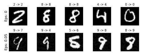
Adversarial attacks are a malicious attack in which an attacker intentionally creates data to cause misclassification in a classifier. Adversarial examples are created by adding a small noise to the input data. An example of adversarial examples is shown in Fig. 1. As shown in Fig. 1, there is no way to distinguish between clean and adversarial samples, but misclassification is caused.

Figure 1: Clean (1st row) and adversarial examples (2nd row)

Adversarial attacks can be classified into non-target attacks and target attacks. In non-target attacks, an attacker tries to make input data misclassify so that it is far away from the original class of the input data. In contrast, in target attacks, an attacker tries to mislead input data to a specified target class. In this paper, we mainly focus on target attacks. In this section, we summarize four adversarial attack methods considered in this paper: fast gradient sign method (FGSM) [2], projected gradient descent (PGD) [16], Jacobian-based saliency map attack (JSMA) [17], and Carlini and Wagner attack (CW) [18].

Figure 2: Procedure of pixel shuffling

FGSM: This is one of the simplest and fastest adversarial attack methods. An attacker linearly fits the cross entropy loss around a target sample, and perturbs input image pixels as maximizing a gradient loss in one-step. FGSM is explained as

$$\begin{split}x_{adv}=x+\epsilon\cdot sign(\nabla_{x}J(\theta,x,y))\end{split}$$ (1)

where $\nabla_{x}J$ is the gradient of a loss function with respect to an original input $x$, $y$ is the ground truth label of $x$, $\epsilon$ is a perturbation added to $x$, and $\theta$ represents classification model parameters.

PGD: PGD is an attack method, which is an extension of FGSM. In FGSM, perturbation $\epsilon$ is added to input $x$ in a single step, while input $x$ is gradually changed with step size $\alpha$ in PGD. The pixel values of a perturbed image are clipped so that they do not change more than $\pm{\epsilon}$ from the original pixel value. PGD attack is shown in the following equation.

$$x_{k+1}=Clip_{(x+\epsilon,x-\epsilon)}(x_{k}+\alpha*sign(\nabla x_{k}))$$ (2)

JSMA: This method is iterative and costly. This attack uses $L_{0}$ norm to attack one or two pixels which cause the largest change in the loss. An input image is attacked by adjusting parameters $\theta$, which represents the magnitude of a perturbation applied to each target pixel, and $\gamma$, which controls the percentage of pixels to be perturbed.

CW: This attack creates an adversarial example by searching for the smallest perturbation computed in $L_{0}$, $L_{1}$, and $L_{2}$ norms. This attack is carried out by controlling parameter $C$ called as confidence. If we set a high value of this parameter, an adversarial example is more different from an original input.

III Proposed detector

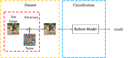
There are two approaches for defending models against adversarial examples. The first approach is to design a classifier that is robust against adversarial attacks as shown in Fig. 3 [2, 5, 6, 7, 8]. This approach includes methods for training models with a dataset including adversarial examples [2], and training models with images transformed with a secret key [8]. The proposed detector includes a robust classifier [2]. Three image transformation methods were used for the robust classifier: pixel shuffling, bit flipping, and format-preserving, feistel-based encryption (FFX). We use pixel shuffling as image transformation to train a robust classifier. Pixel shuffling is carried out in the following steps (see Fig. 2).

1. Split an input image with a size of $h\times w\times c$ into blocks with a size of $M\times M$.

2. Flatten each block into a vector with a length of $M\times M\times c$.

3. Shuffling elements in each vector with a common key $K$ to each block.

4. Merge the transformed blocks.

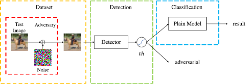
The other approach is to detect adversarial examples just before a classifier as shown in Fig. 4 [10, 11, 12, 13, 14, 15].

Figure 3: Image classification system with robust classifier

Figure 4: Image classification system with adversarial example detector

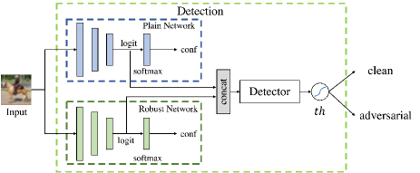
In this paper, we focus on methods for detecting adversarial examples, and propose a novel detection method, which consists of plain and robust classifiers. In the proposed method, it is expected that there is a difference between the output of a plain classifier and that of a robust one if the input image is an adversarial example, as shown in Fig. 5. In other words, the output of a plain classifier is expected to be the same as that of a robust classifier if the input image is clean. The final output from the softmax layer in a classifier, i.e. a confidence value, is represented as a positive value in the range [0,1] for each label. Furthermore, the sum of all confidence values from each classifier is 1. To relax these constraints, in this paper, two logits obtained from the plain classifier and robust classifier are concatenated, and they are used to decide whether an input image is an adversarial example or not, instead of confidence values. The above procedure is summarized in Fig. 6.

(a) Clean samples

(b) Adversarial samples

Figure 5: Assumptions in proposed method

Figure 6: Proposed adversarial detector

IV Experiments

In the experiment, the effectiveness of the proposed detector was evaluated on the basis of two metrics: accuracy (Acc) and area under the curve (AUC), given by Eqs. (3) to (6).

$$Acc =\frac{TP+TN}{TP+FP+TN+FN}$$ (3)

$$TPR =\frac{TP}{TP+FN}$$ (4)

$$FPR =\frac{FP}{TN+FP}$$ (5)

$$AUC =\int TPR\,d(FPR)$$ (6)

These metrics are based on the confusion matrix in binary classification shown in Table I.

TABLE I: Confusion matrix in binary classification

		Predicted
		Positive	Negative
Actual	Positive	True Positive	False Negative
	Negative	False Positive	True Negative

IV-A Experimental setup

We used the CIFAR-10 dataset for testing and training detectors, where the dataset consists of 60,000 images (50,000 images for training, 10,000 images for testing). In the experiment, we assume a white-box attack, and four attacks: FGSM [2], PGD [16], CW [18] and JSMA [17], were applied to input images. We set parameters for each of these attacks as $\epsilon=8/255$ for FGSM and PGD, confidence parameter $C=0$ for CW, and $\theta=1.0,\gamma=0.1$ for JSMA. 8,000 clean images from the test set, and 8,000 adversarial examples generated from the clean images were used to train detectors. The other 2,000 clean images and 2,000 adversarial examples generated from them were used to test a detector. The effectiveness of the proposed detector was compared with Lee’s method [10]. ResNet-18 [19] was used for both a plain classifier and a robust one for the proposed method, and the robust classifier was trained in accordance with Maung’s method [8].

Table II shows the classification performance of the plain and robust classifiers on 10,000 test images under various attacks to show the robustness of the classifiers.

TABLE II: Classification performance of plain and robust classifiers (Noise parameters; $\epsilon=8/255$ for FGSM and PGD. Confidence parameter $C=0$ for CW. $\gamma=0.1$ and $\theta=1.0$ for JSMA)

Classifier	Attack
	CLEAN	FGSM	PGD	CW	JSMA
Plain	0.952	0.557	0.100	0.100	0.104
Robust	0.916	0.812	0.882	0.911	0.743

IV-B Experimental results

In the experiment, the same attacks were used for testing and training detectors.

AUC and Acc scores are shown in Tables III and IV, respectively. From the tables, Lee’s method outperformed the proposed detector under FGSM, but the proposed method outperformed Lee’s method under the other attacks. The reason is that FGSM is not a strong attack as described in Table II, so it is difficult to detect adversarial examples from a difference between the plain and robust classifiers. Adversarial detection methods are required to maintain a high detection accuracy under strong attacks, since weak attacks do not give serious damages in general.

To evaluate how well our detection method can be transferred to unseen attacks, we trained detectors on the features obtained using the CW attack with $C=0$, and then evaluated them on the other (unseen) attacks. Experimental results against the unseen attacks are shown in Table V. It can be observed that our proposed method showed the best performance except to FGSM. Our detection method is based on the output of a plain classifier and that of a robust one, so the proposed detecor is transferable under the condition of using the attacks.

TABLE III: AUC of proposed and Lee’s detectors

Detector	Attack
	FGSM	PGD	CW	JSMA
Lee	0.994	0.983	0.727	0.921
Proposed	0.805	1.000	0.952	0.952

TABLE IV: Acc of proposed and Lee’s detectors

Detector	Attack
	FGSM	PGD	CW	JSMA
Lee	0.990	0.974	0.598	0.865
Proposed	0.740	0.999	0.939	0.942

TABLE V: Acc performance for unseen attacks. Detectors trained with adversarial examples generated by CW attack. (Noise parameters; $\epsilon=8/255$ for FGSM and PGD. Confidence parameter $c=0$ for CW. $\gamma=0.1$ and $\theta=1.0$ for JSMA)

Detector	Attack
	CW(seen)	FGSM(unseen)	PGD(unseen)	JSMA(unseen)
Lee	-	0.971	0.960	0.695
Proposed	-	0.553	0.961	0.940

V Conclusions

In this paper, we propose a detection method for adversarial examples that consists of two image classifiers. In the experiment, the proposed method was confirmed to be able to maintain a high accuracy even under the use of strong attacks. We also showed that our proposed method is robust against unseen attacks under the limited condition.

acknouledgement

This study was partially supported by JSPS KAKENHI (Grant Number JP21H01327)

References

- [1] C. Szegedy, W. Zaremba, I. Sutskever, J. Bruna, D. Erhan, I. Goodfellow, and R. Fergus, “Intriguing properties of neural networks,” in International Conference on Learning Representations (ICLR), Apr. 2014.
- [2] I. Goodfellow, J. Shlens, and C. Szegedy, “Explaining and harnessing adversarial examples,” in International Conference on Learning Representations (ICLR), May. 2015.
- [3] H. Kiya, M. AprilPyone, Y. Kinoshita, I. Shoko, and S. Shiota, “An overview of compressible and learnable image transformation with secret key and its applications,” in arXiv:2201.11006, 2022. [Online]. Available: https://arxiv.org/abs/2201.11006
- [4] M. AprilPyone, Y. Kinoshita, and H. Kiya, “Adversarial robustness by one bit double quantization for visual classification,” IEEE Access, vol. 7, pp. 177 932–177 943, 2019.
- [5] A. Kurakin, I. J. Goodfellow, and S. Bengio, “Adversarial machine learning at scale,” in International Conference on Learning Representations (ICLR), Apr. 2017.
- [6] T. Miyato, S. ichi Maeda, M. Koyama, K. Nakae, and S. Ishii, “Distributional smoothing with virtual adversarial training,” in International Conference on Learning Representations (ICLR), May. 2015.
- [7] F. Tram‘er, A. Kurakin, N. Papernot, I. Goodfellow, D. Boneh, and P. McDaniel, “Ensemble adversarial training: Attacks and defenses,” in International Conference on Learning Representations (ICLR), May. 2018.
- [8] M. AprilPyone and H. Kiya, “Block-wise image transformation with secret key for adversarially robust defense,” IEEE Trans. on Information Forensics and Security, vol. 16, pp. 2709–2723, Mar. 2021.
- [9] M. Aprilpyone and H. Kiya, “Encryption inspired adversarial defense for visual classification,” in IEEE International Conference on Image Processing (ICIP), Oct. 2020, pp. 1681–1685.
- [10] K. Lee, K. Lee, H. Lee, and J. Shin, “A simple unified framework for detecting out-of-distribution samples and adversarial attacks,” in Advances in Neural Information Processing Systems (NIPS), vol. 31, Dec. 2018.
- [11] P. Yang, J. Chen, C.-J. Hsieh, J.-L. Wang, and M. I. Jordan, “Ml-loo: Detecting adversarial examples with feature attribution,” in Association for the Advancement of Artificial Intelligence (AAAI), vol. 34, Feb. 2020, pp. 6639–6647.
- [12] G. Cohen, G. Sapiro, and R. Giryes, “Detecting adversarial samples using influence functions and nearest neighbors,” in IEEE Conference on Computer Vision and Pattern Recognition (CVPR), Jun. 2020, pp. 14 453–14 462.
- [13] A. Higashi, M. Kuribayashi, N. Funabiki, H. H. Nguyen, and I. Echizen, “Detection of adversarial examples based on sensitivities to noise removal filter,” in Asia Pacific Signal and Information Processing Association (APSIPA), Dec. 2020, pp. 1386–1391.
- [14] X. Li and F. Li, “Adversarial examples detection in deep networks with convolutional filter statistics,” in International Conference on Computer Vision (ICCV), Oct. 2017, pp. 5764–5772.
- [15] J. H. Metzen, T. Genewein, V. Fischer, and B. Bischoff, “On detecting adversarial perturbations,” in International Conference on Learning Representations (ICLR), Apr. 2017.
- [16] A. Madry, A. Makelov, L. Schmidt, D. Tsipras, and A. Vladu, “Towards deep learning models resistant to adversarial attacks,” in International Conference on Learning Representations (ICLR), May. 2018.
- [17] N. Papernot, P. D. McDaniel, S. Jha, M. Fredrikson, Z. B. Celik, and A. Swami, “The limitations of deep learning in adversarial settings,” in IEEE European Symposium on Security and Privacy (EuroS&P), Mar. 2016.
- [18] N. Carlini and D. A. Wagner, “Towards evaluating the robustness of neural networks,” in IEEE Symposium on Security and Privacy (SP), May. 2017, pp. 39–57.
- [19] K. He, X. Zhang, S. Ren, and J. Sun, “Deep residual learning for image recognition,” in IEEE Conference on Computer Vision and Pattern Recognition (CVPR), Jun. 2016, pp. 770–778.