Gromov-Wasserstein Discrepancy with Local Differential Privacy
for Distributed Structural Graphs

Abstract

Learning the similarity between structured data, especially the graphs, is one of the essential problems. Besides the approach like graph kernels, Gromov-Wasserstein (GW) distance recently draws a big attention due to its flexibility to capture both topological and feature characteristics, as well as handling the permutation invariance. However, structured data are widely distributed for different data mining and machine learning applications. With the privacy concerns, accessing the decentralized data is limited to either individual clients or different silos. To tackle these issues, we propose a privacy-preserving framework to analyze the GW discrepancy of node embedding learned locally from graph neural networks in a federated flavor, and then explicitly place local differential privacy (LDP) based on Multi-bit Encoder to protect sensitive information. Our experiments show that, with strong privacy protection guaranteed by $\varepsilon$-LDP algorithm, the proposed framework not only preserves privacy in graph learning, but also presents a noised structural metric under GW distance, resulting in comparable and even better performance in classification and clustering tasks. Moreover, we reason the rationale behind the LDP-based GW distance analytically and empirically.

1 Introduction

A lot of applications in machine learning are extensively using either pairwise matrices or kernels to perform the task of prediction or regression. Examples like the RBF kernel and covariance matrices are commonly used in support vector machine classification Chang et al. (2010) in the Euclidean space. However, for the non-Euclidean domains, presented in graphs, such as social network (Fan et al., 2019), recommendation systems (Wu et al., 2020), fraud detection (Li et al., 2020b) and biochemical data (Coley et al., 2019) and topology-aware IoT applications (Abusnaina et al., 2019), involve the study the of relations among the featured objects. To measure the graph similarities, a variety of graph kernels (Borgwardt and Kriegel, 2005; Vishwanathan et al., 2010) are proposed but mainly focus on the topological information. Graph neural networks (GNNs, Kipf and Welling (2016); Hamilton et al. (2017)) are one of the state-of-the-art models to learn node embedding. However, it requires additional readout layers to match the dimension for graph sizes, and it lacks the trackable way to capture the isometric issue on graphs.

Figure 1: Framework

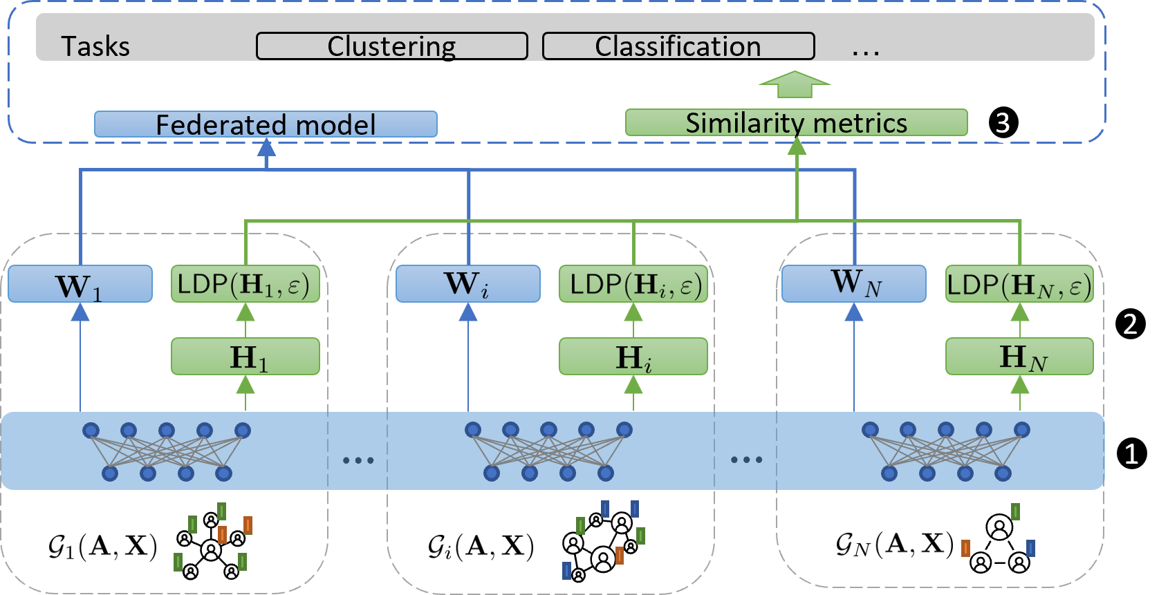
Recently, Gromov-Wasserstein (GW) distance (Mémoli, 2011; Peyré et al., 2016) provides a geometry-based metric to measure the optimal transportation from one structural object to another. GW operates on the metric-measure spaces, i.e., a Borel probability measure on the set with its compact metric space. In other words, it operates on distances between pairs of points calculated within each domain and measures how the distance is compared to those in the other domain. Specifically, all-pair shortest path (APSP) is one of the common geodesic measures applied. Thus, it requires calculating the transportation between two domains by their intra-distance, turning the distance problem from a linear optimization to a quadratic one. And it extends both topological and features information (known as FGW (Titouan et al., 2019)) so that the similarity problem cooperates with the node features nicely. Noting that GW is highly related to graph matching problem, encoding structural information to compare graphs, and has long history been successfully adopted in image recognition (Peyré et al., 2016), bio-domain adoption (Demetci et al., 2020), and point-cloud data alignment (Mémoli and Sapiro, 2006).

One of the key advantages of applying GW distance is the isometric properties between structures. All previous works have assumed that all structured data are always available and accessible, which is often not true in reality. Structured data in many applications either contain sensitive and private information (such as payment transactions and social connections) or distribute across different clients commonly (Liao et al., 2021; Tang et al., 2020). On one hand, data owners are limited to sharing the original data due to the privacy regulations that are enforced globally, such as GDPR Regulation (2018) and CCPA (Bukaty, 2019). On the other hand, in many applications, one has to deal with very large datasets that cannot be processed at once. Thus, a nested partitions of the input which are parameterized by a scale parameter is arising from the metric structure of the input data.

1.1 Problem Formulation

In this paper, we work on the problem of GW distance between distributed graphs while having privacy constraints. Two key assumptions are placed in the underlying such scenarios: 1) each graph holds its topological information, nodes with feature and labels locally; 2) server cannot access raw data globally while having to distinguish from graph to graph (anomaly detection, clustering, recommendation, etc). Accordingly, two main issues need to be addressed: first, to train the global model across different graphs while preserving the privacy of local data; second, to compare graphs even in the case of permutation invariant and size variant. In order to overcome the two issues, we take federated learning schema as our primary framework, along with a geometry-based metric named Gromov-Wasserstein discrepancy (Peyré et al., 2016) on the server-side to learn similarity / dissimilarity across graphs. Gromov-Wasserstein distance (Mémoli, 2011) provides a metric to measure the optimal transportation from one structural object to another.

The proposed framework is illustrated in Figure 1. To summarize: 1) the synchronized vertical federated learning first updates local parameters $\mathbf{\bm{W}}$ from the private structural data $\mathcal{G}(\mathbf{\bm{A}},\mathbf{\bm{X}})$ to learn the local graph embedding $\mathbf{\bm{H}}$; 2) then, instead of pulling the raw graph data from the client, the proposed framework takes the local graph embedding learned from the FL model, and local differential privacy (LDP) is applied explicitly, where we extend the multi-bit encoder from vector space to matrix scenario, protecting the sensitive information; 3) after getting the encoded graph embeddings, the framework calculates similarity metrics (GW distance) on the server and serves the downstream tasks, such as clustering, classification, and matching problems.

Overall, we highlight our core contributions as

• Beyond the conventional federated learning, we design the guaranteed $\varepsilon$-LDP on graph embeddings to explicitly protect the graph information. It is worth mentioning that LDP on topology is not applicable because of the vulnerability of GNN, and perturbation on either the node or edge leads to a non-smoothing function.

• Besides, we adopt the Gromov-Wasserstein discrepancy to be the learnable structural metric on the server, cooperating the LDP encoded graph embeddings from the client-side.

• Interestingly, we observe that the LDP on graph embeddings not only protects privacy but also helps to escape saddle points in GW optimization. We interpret that this is largely due to the non-convexity of GW discrepancy.

• Having the GW discrepancy with noised input, we empirically evaluate the performance of graph classification and clustering problem.

To the best of our knowledge, this is the first work to learn the structural metric with local differential privacy under the distributed setting. And the framework is flexible to learn the node embedding and can be combined with a variety of GNNs for a broad range of different tasks, including graph classification, clustering, etc.

1.2 Notation

We take capital and lower letter in bold to represent matrix and vector, respectively. A graph $\mathcal{G}(\mathbf{\bm{A}},\mathbf{\bm{X}})$ has adjacency matrix $\mathbf{\bm{A}}$ as structural information and node feature $\mathbf{\bm{X}}$ as feature information. Besides, $\mathcal{V},\mathcal{E}$ are the node sets and edge sets from the graph, respectively. $\mathbf{\bm{H}}$ is the retrieved node representation, each row of the matrix represents a single node on the graph. An upper script $(i)$ means the $i$-th graph, while the lower script $i$ means $i$-th row of the matrix.

2 Related Work

The ultimate goal of our proposed method is to protect the privacy of structured data while building the GW distance for similarities between graphs. Naturally, Federated Learning (FL) (McMahan et al., 2017; Smith et al., 2017) is an emerging collaborative learning framework that can train multiple clients locally while maintaining a global model on the server. Distinguished from the shared parameter server Li et al. (2014), one of the significant fruits of federated learning is privacy protection, where each client holds its raw data locally, only shared parameter/gradient will be exchanged with the server. Specifically, in the vertical FL setting, a model is shared among all the clients, and the client trains the model locally with its labels, while the server learns the global models by aggregating the local client models.

Recently, a set of different methods are proposed to build a GNN model with a federated setting. With the task of graph classification, He et al. (2021) design a federated learning system and benchmark for graph neural networks. The framework is built based on FedML (He et al., 2020) research library, enabling to run a variety of GNN models effectively with non-IID graph dataset, which is a similar approach in the image domain. Interestingly, FL-AGCNS (Wang et al., 2021) propose to take advantage of federated learning to accelerate in the task of neural architecture search of graph convolutional network. Specifically, they take federated SuperNet optimization to select random GCN architecture and take federated evolutionary optimization to perform evaluation suing GCN SuperNet.

However, all the work above trains a shared model with the task of supervised/semi-supervised learning, but do not address the issue of unlabelled graphs on clients. What’s more, none of the work above discusses the graph differential privacy while learning the model. Unlike our proposed framework, a recent work of locally private graph neural network (Sajadmanesh and Gatica-Perez, 2020) build the feature and label differential private on the clients at once while leaving the whole training process on the server-side instead.

Another approach to protecting privacy is differential privacy. More specifically, with distributed graphs, we mainly focus on the local differential privacy of each graph. Given a graph $\mathcal{G}(\mathbf{\bm{A}},\mathbf{\bm{X}})$, the purpose of applying LDP is to protect the private information from topology $\mathbf{\bm{A}}$ and node feature $\mathbf{\bm{X}}$. A naive approach would be directly adding LDP noise to $\mathbf{\bm{A}}$ and $\mathbf{\bm{X}}$. However, we argue that such an approach has its limitations. For the topological LDP, assume we add random perturbation to the topology of the graph, i.e., add or delete edges on a graph. However, works like Nettack proposed in Zügner et al. (2018), found that even a small perturbation could lead to the misclassification of the nodes in the graph. Moreover, random perturbation could result in the same graph but is permutation invariant to the original graph, i.e., $\mathbf{\bm{A}}^{\prime}=\Pi(\mathbf{\bm{A}})$, where $\mathbf{\bm{A}}^{\prime}$ is the perturbed graph (Niu et al., 2020). For the feature LDP, adding LDP on feature is a valid approach in the work Sajadmanesh and Gatica-Perez (2020), but it lacks protection for the structural information. Moreover, the study in graph diffusion Wasserstein distance (Barbe et al., 2020) suggests that a noisy feature will let the fused GW depend mostly on the structure. Therefore, adding small random perturbation to either the topology or the feature is not a guaranteed approach to protect privacy in the federated learning setting.

2.1 Gromov-Wasserstein Discrepancy

Graph neural networks rely on training on structured data for various graph-related tasks. However, a common limitation is its difficulty in explaining the isomorphism in graph data. Identification of similarities between graphs is an essential problem in graph learning areas. In these areas, the graph isomorphism problem is known as the exact graph matching (Xu et al., 2019b), which is not solvable in polynomial time nor to be NP-complete. Two graphs are considered isomorphic if there is a mapping between the nodes of the graphs that preserves their adjacencies. The graph isomorphism testing is used in a wide range of applications, such as the identification of chemical compound (Demetci et al., 2020), the generation of molecular graphs in chemical dataset (Titouan et al., 2019), and the electronic design automation (EDA) with placement and routing operations (Chan et al., 2000). Graph Isomorphism Network (GIN) (Xu et al., 2018) is recently proposed to implement Weisfeiler-Lehman (WL) graph isomorphism test (Shervashidze et al., 2011). However, such kind of approach only deals with graphs of the same size, and hard to distinguish the difference between graphs with arbitrary sizes.

Recently, the optimal transport (OT) associated with their Gromov-Wasserstein (GW) discrepancy (Peyré et al., 2016), which extends the Gromov-Wasserstein distance (Mémoli, 2011), has emerged as an effective transportation distance between structured data, alleviating the incomparability issue between different structures by aligning the intra-relational geometries. GW distance is isometric, meaning the unchanged similarity under rotation, translation, and permutation. Formally, Peyré et al. (2016) define the Gromov-Wasserstein discrepancy between two measured similarity matrices $(\mathbf{\bm{C}},\mathbf{\bm{p}})\in\mathds{R}^{n\times n}\times\sum_{n}$ and $(\mathbf{\bm{D}},\mathbf{\bm{q}})\in\mathds{R}^{m\times m}\times\sum_{m}$ as follows

$$\mathsf{GW}(\mathbf{\bm{C}},\mathbf{\bm{D}},\mathbf{\bm{p}},\mathbf{\bm{q}})=\min_{\mathbf{\bm{T}}\in\mathcal{C}_{\mathbf{\bm{p}},\mathbf{\bm{q}}}}\sum_{i,j,k,l}\ell(\mathbf{\bm{C}}_{i,k},\mathbf{\bm{D}}_{j,l})\mathbf{\bm{T}}_{i,j}\mathbf{\bm{T}}_{k,l},$$ (1)

where $\mathbf{\bm{C}}$ and $\mathbf{\bm{D}}$ are matrices representing either similarities or distances between nodes within the graph. $\ell(\cdot)$ is the loss function either in Euclidean norm or KL-divergence (Peyré et al., 2016). $\mathbf{\bm{p}}\in\mathds{R}^{+}_{n}:\sum_{i}\mathbf{\bm{p}}_{i}=1$ is the simplex of histograms with $n$ bins, and $\mathbf{\bm{T}}$ is the coupling between the two spaces on which the similarity matrices are defined. Specifically,

$$\mathcal{C}_{\mathbf{\bm{p}},\mathbf{\bm{q}}}=\left\{\mathbf{\bm{T}}\in\mathds{R}_{+}^{n\times m},\mathbf{\bm{T}}\mathbf{1}=\mathbf{\bm{p}},\mathbf{\bm{T}}^{\top}\mathbf{1}=\mathbf{\bm{q}}\right\},$$

here, we denote the domain $\mathcal{E}:=\left\{\mathbf{\bm{T}}\in\mathds{R}^{n\times m},\mathbf{\bm{T}}\mathbf{1}=\mathbf{\bm{p}},\mathbf{\bm{T}}^{\top}\mathbf{1}=\mathbf{\bm{q}}\right\}$ and $\mathcal{N}:=\mathds{R}_{+}^{n\times m}$. Furthermore, we can rewrite the problem in Koopmans-Beckmann form (Koopmans and Beckmann, 1957):

$$\mathsf{GW}(\mathbf{\bm{C}},\mathbf{\bm{D}},\mathbf{\bm{p}},\mathbf{\bm{q}})=\frac{\left\|\mathbf{\bm{C}}\right\|_{F}^{2}}{n^{2}}+\frac{\left\|\mathbf{\bm{D}}\right\|_{F}^{2}}{m^{2}}-2\max_{\mathbf{\bm{T}}\in\mathcal{C}_{\mathbf{\bm{p}},\mathbf{\bm{q}}}}\mathop{\mathrm{tr}}(\mathbf{\bm{C}}\mathbf{\bm{T}}\mathbf{\bm{D}}\mathbf{\bm{T}}^{\top}).$$ (2)

Note that the $\mathsf{GW}$ distance is non-convex and highly related to the quadratic assignment problem (QAP), which is NP-hard. Therefore, given the similarity matrices $\mathbf{\bm{C}}$ and $\mathbf{\bm{D}}$, we optimize with the quadratic trace form in (2) over the domain of $\mathcal{E}\cap\mathcal{N}$. The GW discrepancy problem can be solved iteratively by conditional gradient method (Peyré et al., 2016) and the proximal point algorithm (Xu et al., 2019a).

In the next section, we will address the details of our proposed $\varepsilon$-LDP on graph embeddings and cooperate them under GW metrics.

3 Framework

To highlight our framework, it encodes node representation from the client while building the structural metric on the server-side. Regarding build the node representation, we train the model in the task of node classification, by using the node labels locally. A conventional federated learning framework is well suited in this setting (detailed description in Appendix E). To the simplification, we take FedAvg as the aggregation algorithm without further notice. Besides, we apply a multi-bit encoder to the node representation as LDP before transmit the graph information to the server. With the protected node representation, server calculates the geometric metric GW accordingly.

3.1 $\varepsilon$-LDP with Multi-bit Encoder on Graph Embedding

Inspired by the locally differential privacy on features, we adopt the multi-bit encoder from Sajadmanesh and Gatica-Perez (2020), while their approach send the encoded feature and label directly to server and train a single model on the server-side. Differentiated from feature encoding, we take the encoder on the node representation, leveraging the privacy on both topology and feature learned from GNN. Algorithm 1 describes the LDP on node embedding in more details. We basically extend the one-bit encoder on a vector space to the multi-bit encoder in 2-D dimension while preserving the guaranteed privacy. Intuitively, the encoder first uniformly sample the $m$ out of the dimension of $n\times h$ without replacement. Then for each row-wise dimension, we take the Bernoulli distribution to decide the mapped encoding after the mask. For each hidden feature dimension, the probability encoding is determined by the number of nodes in the graph ($n$) and the sampled mask ($m$). This is just one-pass encoding with the complexity of $\mathcal{O}(mn)$.

Algorithm 1 $\mathsf{LDP}_{G}(\cdot,\varepsilon)$: Multi-Bit Encoder

Input: Node embedding $\mathbf{\bm{H}}\in\left[\alpha,\beta\right]^{n\times h}$, $\varepsilon$
Output: Encoded embedding $\mathbf{\bm{H}}^{*}$

1:  Let ${\mathcal{S}}$ be a set of $m$ values sampled uniformly from $\left[n\right]\times\left[h\right]$

2:  for $i$ in $n$ do

3:     for $j$ in $h$ do

4:        $s_{ij}=1$ if ${\mathcal{S}}_{ij}=1$ else $s_{ij}=0$

5:        $t_{ij}\sim\text{Bernoulli}\left(\frac{1}{e^{\varepsilon/(mn)}+1}+\frac{\mathbf{\bm{H}}_{ij}-\alpha}{\beta-\alpha}\cdot\frac{e^{\varepsilon/(mn)}-1}{e^{\varepsilon/(mn)}+1}\right)$

6:        $\mathbf{\bm{H}}^{*}_{ij}=s_{ij}(2t_{ij}-1)$

7:     end for

8:  end for

Theorem 1

The multi-bit encoder presented in Algorithm 1 satisfies $\varepsilon$-local differential privacy for each graph representation.

Theorem 1 provides the theoretically guaranteed privacy protection on hidden representation. A detailed proof is provided in the appendix B.

3.2 $\mathsf{GW}$ Distance with LDP on Graph Embeddings

Besides the work of building the global model, we also explicitly enforce the server to construct a pairwise similarity matrix $\mathbf{\bm{C}}\in\mathds{R}^{n\times n}$. More specifically, $\mathbf{\bm{C}}_{\mathbf{\bm{H}}^{*(i)}}\in\mathds{R}^{n^{(i)}\times n^{(i)}}$ represents intra-distance of the encoded node embedding from $i$-th client, namely $\mathbf{\bm{H}}^{*(i)}\in\mathds{R}^{n^{(i)}\times h}$, where $n^{(i)}$ is the number of node in $i$-th graph and $h$ is the hidden dimension. Therefore, we can explicitly formulate the distance matrix between node $u$ and $v$ in $\mathbf{\bm{C}}$ as

$$\mathbf{\bm{C}}_{\mathbf{\bm{H}}^{*}}(u,v)=d(\mathbf{\bm{H}}_{u}^{*},\mathbf{\bm{H}}_{v}^{*}),\ \forall u,v\in\mathcal{V},$$ (3)

where $d(\cdot,\cdot)$ is the distance function applied. Due to its Euclidean space over the reals of $\mathbf{\bm{H}}^{*}$, we can simply take the Euclidean distance between each node embedding to build intra-distance. Of course, it can be easily extended to other distance metrics, such as cosine similarity and correlation. Noting that, after taking the distance introduced from hidden representation, the $\mathbf{\bm{C}}_{\mathbf{\bm{H}}}$ is a metric space induced from the original graph (without $\varepsilon$-LDP encoding). Even though the unbalanced probability measure over nodes are also applicable (Titouan et al., 2019), we will take $\mathbf{\bm{p}}$ as a uniform distribution among the nodes, i.e., $\mathbf{\bm{p}}_{u}=\frac{1}{\left|\mathcal{V}\right|},\forall u\in\mathcal{V}$. Also, as $\mathbf{\bm{H}}$ is the graph representation after federated learning, the embedding itself encodes both structural ($\mathbf{\bm{A}}$) and feature $(\mathbf{\bm{X}})$ information, which is different from the conventional calculating $\mathbf{\bm{C}}$ where only geodesic distance is applied commonly.

Additionally, the framework requires the optimization of Gromov-Wasserstein discrepancy on the server, and the $\varepsilon$-LDP encoded graph embedding can be retrieved only once after a stable global model from FL learning. However, considering the unexpected drop-off of clients, the graph embedding can be retrieved periodically if necessary. Therefore, compared with the vanilla FL setting, sending the encoded graph embedding $\mathbf{\bm{H}}^{*}$ will not introduce overhead in communication.

4 Experiments

Dataset

We will perform two tasks, one with graph classification under federated learning via GW, where we take the benchmark datasets from TUDataset (Morris et al., 2020). Another task is to take the graph clustering with subgraph generated from the single big graph, where we take the citation benchmark dataset from Planetoid (Yang et al., 2016). Detailed statistics of the dataset and settings of hyperparameters are included in the appendix C.

Graph classification

Model	Metric Source	PROTEINS	MUTAG	IBMD-B
SPK	$\mathbf{\bm{A}}$	n/a	82.95 $\pm$ 8.19	55.80 $\pm$ 2.93
GCN	$\mathbf{\bm{A}}\mathbf{\bm{X}}$	69.03 $\pm$ 3.59	80.05 $\pm$ 3.21	n/a
SVM	$\mathsf{GW}_{\mathbf{\bm{A}}}/\mathsf{FGW}_{\mathbf{\bm{A}}\mathbf{\bm{X}}}$	74.55 $\pm$ 2.74	83.26 $\pm$ 10.3	63.8 $\pm$ 3.49
SVM	$\mathsf{GW}_{\mathbf{\bm{H}}(GCN)}$	72.31 $\pm$ 4.61	80.3 $\pm$ 9.75	53.69 $\pm$ 4.31
SVM	$\mathsf{GW}_{\mathbf{\bm{H}}^{*}(GCN)}$	71.19 $\pm$ 3.92	79.57 $\pm$ 6.73	54.01 $\pm$ 4.90
SVM	$\mathsf{GW}_{\mathbf{\bm{H}}(GIN)}$	75.53 $\pm$ 2.01	93.08 $\pm$ 3.35	74.4 $\pm$ 1.11
SVM	$\mathsf{GW}_{\mathbf{\bm{H}}^{*}(GIN)}$	76.89 $\pm$ 3.90	91.17 $\pm$ 4.21	73.6 $\pm$ 3.23

Table 1: Accuracy on graph classification

Regarding the task of graph classification under a centralized setting, we adopt an SVM using the indefinite kernel matrix $e^{-\gamma\mathsf{FGW}}$ as a distance between graphs (Titouan et al., 2019), where the training, validation, and testing sets are split in the ratio of $7:2:1$. For all methods using SVM, we cross validate the parameter $C\in\left\{10^{-7},10^{-6},\cdots,10^{7}\right\}$ and $\gamma\in{2^{-10},2^{-9},\cdots,2^{10}}$. For the decentralized setting, we split the graphs into 10 clients from the Dirichlet distribution (Wang et al., 2020), and each client has 20% and 10% for validation and testing, respectively. We report the classification accuracy in Table 1. Both PROTEINS and MUTAG has node features, where we adopt the $\mathsf{FGW}$ as the base metric. While IMDB-B has no features on nodes, we only take the GW (topology only) as the base metric. SPK Borgwardt and Kriegel (2005) is the shortest path kernel method on raw data. GCN indicates a two-layer graph convolutional layer with hidden dimension of 16, followed by an average pooling method. GIN represent a five graph isomorphic layers with hidden dimension of 64, followed by a two linear perception layers.

Comparing the results from raw data (metric based on $\mathbf{\bm{A}},\mathbf{\bm{X}}$), we can see the kernel based SVM on GW discrepancy performs better than the base GCN and SPK model. For the FL setting, we defined the shared model with GCN and GIN. $\mathbf{\bm{H}}$ is the graph embedding without privacy protection, and $\mathbf{\bm{H}}^{*}$ is $\varepsilon$-LDP graph embedding. Without the further notice, we take the optimal $m^{*}=\max(1,\min(d,\left\lfloor\frac{\varepsilon}{2.18}\right\rfloor))$ from Sajadmanesh and Gatica-Perez (2020), and $d$ is the number of classes from nodes. We exact the node embedding based after the softmax layer, leaving $\alpha=0,\beta=1$. The default value is $\varepsilon={\textstyle\frac{1}{\left|\mathcal{V}\right|}}$ which varies from each graph. Intuitively, this basically means the cumulative privacy budget will be normalized on the number of nodes $n$.

To see the effectiveness of FL, GCN model under FL perform a bit worse than SVM on raw data. However, FL under GIN (a strong model) improves almost 10% when compared with vanilla SVM with raw data. What’s more, to check how LDP works (using the $\mathbf{\bm{H}}^{*}$ graph embedding) in the classification tasks, we can find that the $\varepsilon$-LDP didn’t hurt the overall performance.

Graph clustering

Our framework fits unsupervised learning with federated learning. And it is quite common to see that labels for each node are trivial, but not for the subgraphs (communities). Regarding the data with a single graph, we split the big graph into small subgraphs by taking multi-hop neighbors for simplification. Moreover, for such kind of dataset, we might not have the ground-truth label of the split subgraph. Therefore, we take the label of the central node as its pseudo-label. To note, we will see the overlap of nodes in different clients, which is a typical scenario in various applications, such Internet-of-Things (IoT) devices, community connections, and recommendation systems. A shared 2-layer GCN model with node classification task is deployed in the federated setting, where each client builds the node embedding. We retrieve the node embedding after a fixed number of 200 rounds of updating the shared model.

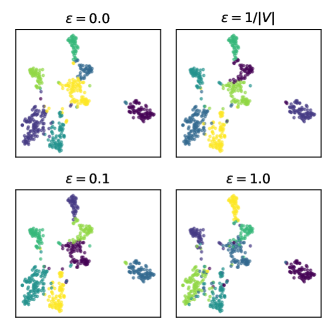
Figure 2 shows the t-SNE plot of KMeans clustering of 500 1-hop subgraphs from citeseer dataset with different $\varepsilon$. KMeans under GW distance is different from Euclidean distance, the centroid of each cluster is represented by a metric matrix. To simplify, we fix the dimension of the centroid by the average number of nodes within the cluster. Noting that $\varepsilon=0$ means no LDP introduced to the graph embedding and we assume the number of clusters is equal to the number of labels from nodes. Intuitively, data in the citation network has the label for each paper, and the induced subgraph is the citations referred for the central node. To see the impact of GW distance in clustering, comparing the first and second plots in Figure 2 shows that even without the LDP encoder, the KMeans clustering with GW distance performance better than the naive labeling from central node. Thanks to the property of GW distance, it provides a better similarity metrics, especially having a pre-learned graph embeddings. To see the impact of LDP in clustering, compared with the raw graph embedding, the encoded $\mathbf{\bm{H}}^{*}$ with small $\varepsilon$ won’t hurt too much in the clusters. However, a larger privacy strength ($\varepsilon=1$) introduces more deviates of unlabelled subgraphs. This is consistent with the observation in classification problem as well. Additional results with 2-hop subgraphs and other datasets are provided in Appendix C. In the next subsection, we will have a close look at privacy strength $\varepsilon$ in the GW distance calculation.

Figure 2: Clustering on subgraphs based on $\mathsf{GW}$. Pseudo label comes from the central node.

4.1 Privacy analysis for LDP on embedding

Figure 3: Cross validation on $\varepsilon$ with KNN model (left: $k=5$, right: $k=20$).

Figure 4: A demonstration of LDP on node embedding for GW metric.

Knowing that the $\varepsilon$ is a key factor in privacy protection and downstream tasks, we invest the impact of privacy budget $\varepsilon$ in LDP under classification. Following the Figure 3, in order to eliminate the influence of hyperparameter in GNN models, we report the accuracy using KNN based on $\mathsf{GW}_{\mathbf{\bm{H}}^{*}}$ by cross-validating on $\varepsilon$ on MUTAG dataset. As we can see on both settings of $k=5,20$, the model is relative stable with just a small perturbation, i.e., $\varepsilon<1$, and with the increased privacy protection strength, a larger $\varepsilon$ will hurt the overall performance. More interestingly, by introducing the $\varepsilon$-LDP, it not only helps to protect the privacy, but also potentially helps the performance in downstream tasks with a proper $\varepsilon$.

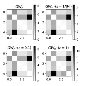
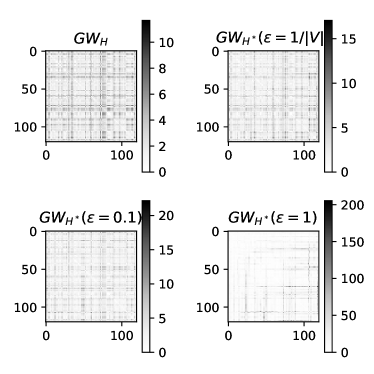
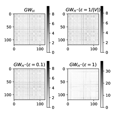
Furthermore, we look into details of changes in similarity metric $\mathsf{GW}$ distance with respect to the $\varepsilon$. For the task of clustering, we extract five subgraphs (check Appendix D for subgraph structures) from citeseer dataset, and shows the results of $\mathsf{GW}$ discrepancy when LDP is applied with different $\varepsilon$ in Figure 4. We consider two privacy budgets $\varepsilon=0.1,1$ to be compared. $\mathsf{GW}_{H}$ represents the distance without LDP, i.e., $\varepsilon=0$, with the baseline statistics of $\mathsf{GW}$ discrepancy to be $2.38\pm 2.22$. $\mathsf{GW}_{H^{*}}$ represents the distance under encoded LDP with three different privacy budget $\varepsilon={\textstyle\frac{1}{\left|\mathcal{V}\right|}},0.1,1$, and $2.42\pm 2.33$, $2.43\pm 2.35$, $3.25\pm 3.09$ are the distances statistics, respectively. It can be seen from Figure 4, with a proper privacy budget, we can see little difference on pairwise distance based on $\mathsf{GW}$. In other words, from the perspective of applications, with LDP on node embedding has little affection for the clustering / classification tasks. It is also true from the algorithmic view that $\mathsf{GW}$ distance is quantitatively stable (Mémoli, 2011) in the sense of the structure invariant. Moreover, in the distributed training, graphs are completely in non-i.i.d. distribution, suggesting that the $\varepsilon$ can vary from client to client. Therefore, we have our default $\varepsilon$ set to be $1/\left|\mathcal{V}\right|$, which also matches our design of algorithm 1, sampling based on number of nodes. We also provide an insightful explanation of taking GW distance when comparing with other graph similarity metrics in Appendix D

4.2 Rationale behind GW with $\varepsilon$-LDP encoder

We step further to reason why the LDP on $\mathbf{\bm{H}}$ won’t sacrifice the $\mathsf{GW}$ distance. Due to the non-convexity of GW discrepancy, which involves a quadratic problem, the absolute error in distance from different pairs cannot have a guaranteed boundary to tell the closeness between them. Despite the challenge of finding the exact the global minima, an effective way is to escape saddle points in the non-convex manifold, which prevents the optimal solution to be stuck at the local minima.

Figure 5: Averaged GW discrepancy (optimal function value) with the increase of $\varepsilon$. Left: graphs induced from 1-hop neighbors. Right: graphs induced from 2-hop neighbors.

Among many of the works targeting the escape saddle points, perturb gradient descent (PGD) Jin et al. (2017) is one of practical simple method to solve the problem. The meta-algorithm is described as

$$\mathbf{\bm{x}}_{t}\leftarrow\mathbf{\bm{x}}_{t}+\mathbf{\bm{\xi}}_{t},\quad\quad\mathbf{\bm{x}}_{t+1}\leftarrow\mathbf{\bm{x}}_{t}-\eta{\nabla}f(\mathbf{\bm{x}}_{t})$$ (4)

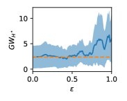
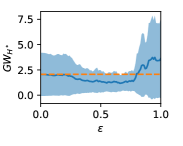
where $\mathbf{\bm{\xi}}_{t}\sim\mathcal{B}(\varepsilon)$ is a small perturbation on the input space within a small ball. Noting that, the $\mathbf{\bm{H}}^{*}=\mathbf{\bm{H}}+\mathcal{O}(\varepsilon)$ and $\mathbf{\bm{C}}_{u,v}=d(\mathbf{\bm{H}}^{*}_{u},\mathbf{\bm{H}}^{*}_{v})=d(\mathbf{\bm{H}}_{u},\mathbf{\bm{H}}_{v})+\mathcal{O}(\varepsilon)$, when $d$ is a Euclidean distance function. Interestingly, we can take the LDP as small perturbation on the node embedding, which is ultimately the noisy input to the GW optimization problem. Lacking of exact tracking the impact of noise in optimization, we empirically check the average output of GW with the increase of the $\varepsilon$. Figure 5 indicates the average GW discrepancy calculated by increasing the privacy budget $\varepsilon$ on the dataset Citeseer. We fix the initial point and other hyperparameters (threshold, max iter and etc.) in optimization, the only differences are $\varepsilon$. The solid blue curve indicates the average GW discrepancy (optimal function value) and the dashed orange line indicate the baseline without any perturbations. Although the increase of the privacy budget $\varepsilon$ eventually leads to a higher mean and variance of GW discrepancy which is expected, a slight perturbation from LDP (when $\varepsilon$ is small) helps to get a lower GW discrepancy (smaller optimal function value from blue curve), especially when the graph is more complicated (2-hop neighbors).

The empirical result matches with our understand of non-convex optimization with perturbed method. However, a rigorous analysis of relation between LDP and non-convex still remains unclear, especially in the connection between privacy budget and the constrained perturbation domain. We will leave this problem for our further work.

5 Conclusion

In this paper, we propose a novel framework to protect the distributed structural graphs by introducing the local differential privacy to graph embeddings and handle the permutation invariant issue by taking the Gromov-Wasserstein distance for further downstream tasks. With the guaranteed $\varepsilon$-LDP encoding on graph embedding, our experiment shows that the privacy budget not only helps in the distributed privacy protection learning, but also won’t hurt the performance of the downstream tasks. We also invest the reasons behind it, thanks to the non-convexity of $\mathsf{GW}$ distance, the additional noise in LDP is not a burden in the downstream tasks. Considering the flexibility of the framework, an interesting extension is to see the performance on large heterogeneous graphs, where the subgraphs represent small communities in social networks, fraud actions in transactions networks, and browsing logs in recommendation systems.

Appendix A Definition of LDP

Definition 1 (LDP (Dwork et al., 2014))

Let $\mathcal{A}:\mathcal{D}^{n}\Rightarrow\mathcal{Z}$ be a randomized algorithm mapping a dataset with $n$ records to some arbitrary range $\mathcal{Z}$. The algorithm $\mathcal{A}$ is $\varepsilon$-local differential privacy if it can be written as $\mathcal{A}(d^{(1)},\cdots,d^{(n)})=\Phi(\mathcal{A}_{1}(d^{(1)},\cdots,\mathcal{A}_{n}(d^{(n)})))$, where each $\mathcal{A}_{i}:\mathcal{D}\rightarrow\mathcal{Y}$ is an $\varepsilon-$local randomizer for each $i\in\left[n\right]$ and $\Phi:\mathcal{Y}^{n}\rightarrow\mathcal{Z}$ is some post-processing function of the privatized records $\mathcal{A}_{1}(d^{(1)},\cdots,\mathcal{A}_{n}(d^{(n)}))$. Note that the post-processing function does not have access to the raw data records.

Appendix B Proof of Theorem 1

Proof:  Let $\mathcal{M}(\mathbf{\bm{H}})$ to be the multi-bit encoder as described in Algorithm 1. Let $\mathbf{\bm{H}}^{*}$ be the perturbed node embedding corresponding to $\mathbf{\bm{H}}$. We need to show that for any two embeddings $\mathbf{\bm{H}}$ and $\mathbf{\bm{H}}^{\prime}$, we have $\ln{\frac{\mathsf{P}\left[\mathcal{M}(\mathbf{\bm{H}})=\mathbf{\bm{H}}^{*}\right]}{\mathsf{P}\left[\mathcal{M}(\mathbf{\bm{H}}^{\prime})=\mathbf{\bm{H}}^{*}\right]}}\leq\varepsilon$. According to Algorithm 1, for each row-wise vector representation, we have seen that $\mathbf{\bm{H}}_{i,:}^{*}\in\left\{-1,0,1\right\}$ and the case of $\mathbf{\bm{H}}_{i,:}^{*}=0$ occurs when $i\notin{\mathcal{S}}$. Therefore, we have

$$\ln\frac{\mathsf{P}\left[\mathcal{M}(\mathbf{\bm{H}}_{i,:})=0\right]}{\mathsf{P}\left[\mathcal{M}(\mathbf{\bm{H}}^{\prime}_{i,:})=0\right]}=\ln\frac{1-(mn)/h}{1-(mn)/h}=0\leq\varepsilon,$$ (5)

for all $\varepsilon>0$ and $i\in\left[n\right]$. In the case of $\mathbf{\bm{H}}_{i,:}^{*}\in\left\{-1,1\right\}$, we see that the probability of getting $-1$ or $1$ ranges from $\frac{(mn)}{h}\cdot\frac{1}{e^{\varepsilon/(mn)}+1}$ to $\frac{(mn)}{h}\cdot\frac{e^{\varepsilon/(mn)}}{e^{\varepsilon/(mn)}+1}$. Then we have

$$\frac{\mathsf{P}\left[\mathcal{M}(\mathbf{\bm{H}}_{i,:})\in\left\{-1,1\right\}\right]}{\mathsf{P}\left[\mathcal{M}(\mathbf{\bm{H}}^{\prime}_{i,:})\in\left\{-1,1\right\}\right]}\leq\frac{\max\mathsf{P}\left[\mathcal{M}(\mathbf{\bm{H}}_{i,:})\in\left\{-1,1\right\}\right]}{\min\mathsf{P}\left[\mathcal{M}(\mathbf{\bm{H}}^{\prime}_{i,:})\in\left\{-1,1\right\}\right]}$$

$$= \left(\frac{(mn)}{h}\cdot\frac{e^{\varepsilon/(mn)}}{e^{\varepsilon/(mn)}+1}\right)/\left(\frac{(mn)}{h}\cdot\frac{1}{e^{\varepsilon/(mn)}+1}\right)=e^{\varepsilon/(mn)}.$$

Then by the composition theorem, we have

$$\frac{\mathsf{P}\left[\mathcal{M}(\mathbf{\bm{H}})=\mathbf{\bm{H}}^{*}\right]}{\mathsf{P}\left[\mathcal{M}(\mathbf{\bm{H}}^{\prime})=\mathbf{\bm{H}}^{*}\right]} =\prod_{i=1}^{n}\prod_{j=1}^{h}\frac{\mathsf{P}\left[\mathcal{M}(\mathbf{\bm{H}}_{ij})=\mathbf{\bm{H}}_{ij}^{*}\right]}{\mathsf{P}\left[\mathcal{M}(\mathbf{\bm{H}}_{ij}^{\prime})=\mathbf{\bm{H}}_{ij}^{*}\right]}$$

$$\leq\prod_{i=1}^{n}\prod_{\mathbf{\bm{H}}^{*}_{ij}\in\left\{-1,1\right\}}e^{\varepsilon/(mn)}\leq e^{\varepsilon},$$

which concludes the proof of $\varepsilon$-d.p.  

Appendix C More experiments

We take the experiments in two scenarios: one with single graph, but split into multiple subgraphs; the other takes the standard graph classification benchmark. Table 2 and Table 3 are the statistics of those datasets. Table 4 is the statistics of induced subgraphs from citation networks.

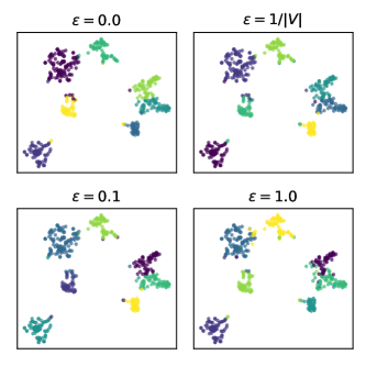
To compare the impact of graph sizes when applying the $\varepsilon$-LDP, Figure 6 show the result from 1-hop and 2-hop subgraphs. where the pseudo label comes from the central node of the subgraph. As we can see, the GW based kmeans works better than the vanilla labeling. With a slight increase of $\varepsilon$, there will be a good performance in clustering. However, with a significant large privacy strength, it will introduce more deviates from the centroid. We also provide the clustering result from another dataset Cora in Figure 7.

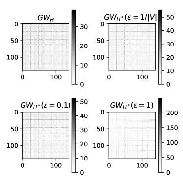
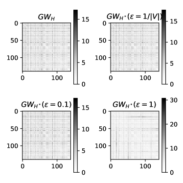
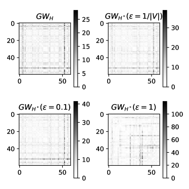
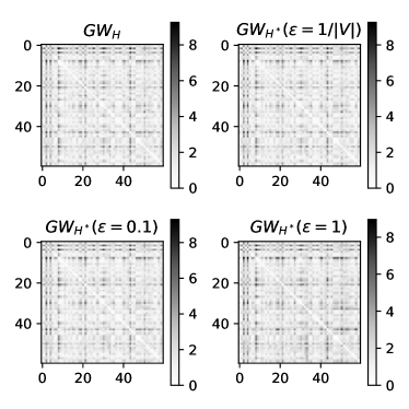
For the GW metric with LDP in subgraphs, we take all the training nodes as the central node, and present GW metric with LDP under different buget with both 1-hop and 2-hop induced subgraphs. Figure 8,9,10 are the GW metric with LDP from citeseer, cora and pubmed, respectively.

Figure 6: Clustering from 1-hop (top) and 2-hop (bottom) subgraphs of citeseer

(a)

(b)

Figure 7: Cora

Dataset	$\left|\mathcal{V}\right|$	$\left|\mathcal{E}\right|$	avg. degree	feature dim	num of labels
Citeseer	2120	3679	3.47	3703	6
Cora	2485	5069	4.08	1433	7
Pubmed	19717	44324	4.50	500	3

Table 2: Single Graph Datasets

Dataset	num of graphs	node feature	num of label	avg nodes	avg edges
PROTEINS	1113	32	2	39.06	145.63
MUTAG	188	7	2	17.93	39.58
IMDB-Binary	1000	0	2	19.77	193.06

Table 3: Multl-graph Dataset

Dataset	hop	avg. nodes	avg. edges	avg. degree
Citeseer	1	4.61	5.15	1.8
	2	25.13	44.26	2.58
Cora	1	5.77	7.32	2.16
	2	49.15	89.46	2.95
Pubmed	1	5.95	6.65	1.66
	2	53.83	103.95	2.82

Table 4: Statistics of split subgraphs

(a)

(b)

Figure 8: Citeseer

(a)

(b)

Figure 9: Cora

(a)

(b)

Figure 10: Pubmed

Appendix D Similarity Measures.

To demonstrate the advantage of using Gromov-Wasserstein distance, we compare it with other graph metrics,

Figure 11: A demonstration of pairwise distance with different metrics. Five graphs in the upper row are the subgraph retrieved by 1-hop neighbors. Pairwise distances are presented in the second row. Both $GED$ and $GW_{A}$ are calculated from the structure information only, while $FGW_{AX}$ has both structure and feature involved when we set $\alpha=0.5$. $GW_{H}$ is the new pairwise distance evaluated from the node embedding.

• Graph edit distance on topology. Graph edit distance (GED) is a measure of similarity between two graphs in the fashion of their topology by summing over these optimal operations of insertion, deletion, and substitution for both nodes and edges. However, the exact calculation of GED is NP-hard (Zeng et al., 2009). Here, we adopt the exponential algorithm from Abu-Aisheh et al. (2015) to calculate the GED for pairwise graphs.

• Gromov-Wasserstein distance on topology. We follow the setup in Eq.2, where optimal transportation is calculated based on graph topology. Regarding the structure distance $\mathbf{\bm{C}}$, they are computed by considering an all-pair shortest path (APSP) between the vertices.

• Fused Gromov-Wasserstein distance on topology and node features. Fused-GW ($\mathsf{FGW}$) (Titouan et al., 2019) is an extension to the vanilla $\mathsf{GW}$, in order to cooperate with node feature as well. More specifically, it defines a trade-off parameter $\alpha\in\left[0,1\right]$ between the feature and structure distance.

• Gromov-Wasserstein discrepancy on node embedding. Besides the distance calculate directly from the raw data, we also calculate the discrepancy based on the hidden representation as defined in Eq.6.

Figure 11 provides an insightful view of the pairwise distance under different metrics. We randomly take five subgraphs induced from the 1-hop neighbors from Citeseer dataset, and the label from the central node is marked. Note that the first and second graphs have the same pseudo-label, and the first and the fifth graphs are isomorphic to each other. $GED$, $GW_{A}$, and $FGW_{AX}$ fail to detect similar properties from the first and second graphs. And for the isomorphism, thanks to the GW discrepancy, $GW_{H}$ is able to recognize the difference between those two graphs. Noting that $GED$, $GW_{A}$ has the topological information only, while $FGW_{AX}$ and $GW_{H}$ encode both structure and feature, while $GW_{H}$ has the additional learning process.

Appendix E Federate learning

Server-side.

Under the federated learning setting, we take the aggregation algorithm $\mathsf{AGG}$ to build a global model in each round (line 11) as shown in Algorithm 2. Algorithms like FedAvg (McMahan et al., 2017), FedProx (Li et al., 2020a), and MFL Liu et al. (2020) can be applied accordingly. Moreover, it also allows the server to adopt secure aggregators (Bonawitz et al., 2016; So et al., 2020; Li et al., 2019) to improve the robustness of the global model.

Besides the work of building the global model, we also explicitly enforce the server to construct a pairwise similarity matrix $\mathbf{\bm{D}}\in\mathds{R}^{N\times N}$ (line 12 in Algorithm 2), which can be used for pipeline applications (Alvarez-Melis and Jaakkola, 2018; Peyré et al., 2016; Demetci et al., 2020). $\mathbf{\bm{C}}_{\mathbf{\bm{H}}^{(i)}}\in\mathds{R}^{n^{(i)}\times n^{(i)}}$ represents intra-distance of the node embedding from $i$-th client, namely $\mathbf{\bm{H}}^{(i)}\in\mathds{R}^{n^{(i)}\times h}$, where $n^{(i)}$ is the number of node in $i$-th graph and $h$ is the hidden dimension. Therefore, we can explicitly formulate the distance matrix between node $u$ and $v$ in $\mathbf{\bm{C}}$ as

$$\mathbf{\bm{C}}_{\mathbf{\bm{H}}}(u,v)=d(\mathbf{\bm{H}}_{u},\mathbf{\bm{H}}_{v}),\ \forall u,v\in\mathcal{V},$$ (6)

where $d(\cdot,\cdot)$ is the distance function applied. Due to its Euclidean space over the reals of $\mathbf{\bm{H}}$, we can simply take the Euclidean distance between each node embedding to build intra-distance. Of course, it can be easily extended to other distance metrics, such as cosine similarity and correlation. Noting that, after taking the distance introduced from hidden representation, the $\mathbf{\bm{C}}_{\mathbf{\bm{H}}}$ is a metric space induced from the original graph. Even though the unbalanced probability measure over nodes are also applicable (Titouan et al., 2019), we will take $\mathbf{\bm{p}}$ as a uniform distribution among the nodes, i.e., $\mathbf{\bm{p}}_{u}=\frac{1}{\left|\mathcal{V}\right|},\forall u\in\mathcal{V}$.

Additionally, the framework requires the optimization of Gromov-Wasserstein discrepancy on the server and can be retrieved only once after a stable global model. However, considering the unexpected drop-off of clients, we enforce the model to retrieve the encoded embedding periodically (parameter $s$).

Client-side.

After get initial model from the server, the local client take full-batch training to update local model. $f(\cdot)$ is a shared GNN model with server. As we describe earlier, we also explicitly take the local differential privacy on node embeddings. By taking so, the raw data is protected, and also by taking the GNN, it is an implicit way to protect graph information. What’s more, it secures the embedding with LDP privacy guaranteed, which again protect the raw data while sharing encoded embedding with the server. We provide our framework in Algorithm 2, 3.

Algorithm 2 Server’s work

Input: Initial model $\mathbf{\bm{w}}$
Parameter: periodic signal $s$, rounds $R$, number of clients $N$
Output: global model $\widetilde{\mathbf{\bm{w}}}$, pairwise distance $\mathbf{\bm{D}}$

1:  $\widetilde{\mathbf{\bm{w}}}_{0}=\mathbf{\bm{w}}$

2:  for $r$ in $1\cdots R$ do

3:     for $i$ in $1\cdots N$ do

4:        Send $\widetilde{\mathbf{\bm{w}}}_{r-1}$ to clients

5:        if $s$ then

6:           $\mathbf{\bm{w}}^{(i)},\mathbf{\bm{H}}^{(i)}\leftarrow$ update on local client $i$

7:        else

8:           $\mathbf{\bm{w}}^{(i)}\leftarrow$ update on local client $i$

9:        end if

10:     end for

11:     $\widetilde{\mathbf{\bm{w}}}_{r}\leftarrow\mathsf{AGG}(\mathbf{\bm{w}}^{(i)},\forall i\in N)$

12:     $\mathbf{\bm{D}}\leftarrow\mathsf{GW}(\mathbf{\bm{C}}_{\mathbf{\bm{H}}^{(i)}},\mathbf{\bm{C}}_{\mathbf{\bm{H}}^{(j)}},\mathbf{\bm{p}}^{(i)},\mathbf{\bm{p}}^{(j)}),\forall i,j\in N^{2}$

13:  end for

14:  return $\widetilde{\mathbf{\bm{w}}}_{r},\mathbf{\bm{D}}$

Algorithm 3 Client’s work

Input: Local graph $\mathcal{G}(\mathbf{\bm{A}},\mathbf{\bm{X}})$, global model $f(\widetilde{\mathbf{\bm{w}}})$
Parameter: local epoch $E$, periodic signal $s$, LDP privacy $\varepsilon$
Output: Updated model $\mathbf{\bm{w}}^{(l)}$, node embedding $\mathbf{\bm{H}}^{(l)}\in\mathds{R}^{n\times h}$

1:  $\mathbf{\bm{w}}_{0}=\widetilde{\mathbf{\bm{w}}}$

2:  for $e$ in $1\cdots E$ do

3:     Full-batch training to update $\mathbf{\bm{w}}_{e}\leftarrow f(\mathbf{\bm{A}},\mathbf{\bm{X}},\mathbf{\bm{w}}_{e-1})$

4:  end for

5:  $\mathbf{\bm{w}}^{(l)}=\mathbf{\bm{w}}_{e}$

6:  if $s$ then

7:     $\mathbf{\bm{H}}^{(l)}\leftarrow\mathsf{LDP}_{G}\left(f(\mathbf{\bm{A}},\mathbf{\bm{X}},\mathbf{\bm{w}}^{(l)}),\varepsilon\right)$

8:  end if

9:  return $\mathbf{\bm{w}}^{(l)},\mathbf{\bm{H}}^{(l)}$ if $s$.

Appendix F Differential privacy on graphs

Differential privacy on graphs imposes a restriction of algorithms to protect the information of structured data. More specifically, such kind of algorithm helps to protect the statistics of graph, such as subgraph counts, number of edges and degree distribution (Kasiviswanathan et al., 2011).

There are two kinds of differential privacy on graph, edge and node differential privacy. For the edge differential privacy, two graphs are neighbors if they differ exactly one edge, and the purpose is to protect the relation of entities in the graph. For the node differential privacy, two graphs are neighbors if they differ exact one node and its associated edges. We empirically study the difference when having an exact one edge/node difference. As mentioned earlier, LDP on topology is not a trivial roadmap in the GNN setting, especially the node DP has more influence on the difference due to the potential changes not only in nodes but also in its associated edges.

Figure 12: Difference in GW after exact one edge/node difference.

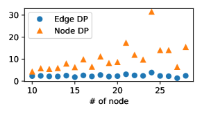
More specifically, given a graph $\mathcal{G}$, we are interested in how the GW changes when comparing two neighbor graphs, $d=\left|\mathsf{GW}(\mathcal{G}^{\prime},\mathcal{G})\right|$, where $\mathcal{G}^{\prime}$ and $\mathcal{G}$ differ only one edge or node. We take the MUTAG dataset TUDataset Morris et al. (2020) as an example. For each sample graph in the dataset, we show that the directly topology differential privacy has a diverse difference, especially for the graph neighbors in terms of nodes.

References

- Abu-Aisheh et al. [2015] Zeina Abu-Aisheh, Romain Raveaux, Jean-Yves Ramel, and Patrick Martineau. An exact graph edit distance algorithm for solving pattern recognition problems. In ICPRAM, 2015.
- Abusnaina et al. [2019] Ahmed Abusnaina, Aminollah Khormali, Hisham Alasmary, Jeman Park, Afsah Anwar, and Aziz Mohaisen. Adversarial learning attacks on graph-based iot malware detection systems. In ICDCS, pages 1296–1305. IEEE, 2019.
- Alvarez-Melis and Jaakkola [2018] David Alvarez-Melis and Tommi Jaakkola. Gromov-wasserstein alignment of word embedding spaces. In Proceedings of the 2018 Conference on Empirical Methods in Natural Language Processing, pages 1881–1890, 2018.
- Barbe et al. [2020] Amélie Barbe, Marc Sebban, Paulo Gonçalves, Pierre Borgnat, and Rémi Gribonval. Graph diffusion wasserstein distances. In ECML, 2020.
- Bonawitz et al. [2016] Keith Bonawitz, Vladimir Ivanov, Ben Kreuter, Antonio Marcedone, H Brendan McMahan, Sarvar Patel, Daniel Ramage, Aaron Segal, and Karn Seth. Practical secure aggregation for federated learning on user-held data. arXiv preprint arXiv:1611.04482, 2016.
- Borgwardt and Kriegel [2005] Karsten M Borgwardt and Hans-Peter Kriegel. Shortest-path kernels on graphs. In ICDM, pages 8–pp. IEEE, 2005.
- Bukaty [2019] Preston Bukaty. The California Consumer Privacy Act (CCPA): An Implementation Guide. IT Governance Publishing, 2019.
- Chan et al. [2000] Tony F Chan, Jason Cong, Tianming Kong, and Joseph R Shinnerl. Multilevel optimization for large-scale circuit placement. In ICCAD, pages 171–176. IEEE, 2000.
- Chang et al. [2010] Yin-Wen Chang, Cho-Jui Hsieh, Kai-Wei Chang, Michael Ringgaard, and Chih-Jen Lin. Training and testing low-degree polynomial data mappings via linear svm. JMLR, 11(4), 2010.
- Coley et al. [2019] Connor W Coley, Wengong Jin, Luke Rogers, Timothy F Jamison, Tommi S Jaakkola, William H Green, Regina Barzilay, and Klavs F Jensen. A graph-convolutional neural network model for the prediction of chemical reactivity. Chemical science, 10(2):370–377, 2019.
- Demetci et al. [2020] Pinar Demetci, Rebecca Santorella, Bjorn Sandstede, William Stafford Noble, and Ritambhara Singh. Gromov-wasserstein optimal transport to align single-cell multi-omics data. BioRxiv, 2020.
- Dwork et al. [2014] Cynthia Dwork, Aaron Roth, et al. The algorithmic foundations of differential privacy. FTTCS, 9(3-4):211–407, 2014.
- Fan et al. [2019] Wenqi Fan, Yao Ma, Qing Li, Yuan He, Eric Zhao, Jiliang Tang, and Dawei Yin. Graph neural networks for social recommendation. In The World Wide Web Conference, pages 417–426, 2019.
- Hamilton et al. [2017] William L Hamilton, Rex Ying, and Jure Leskovec. Inductive representation learning on large graphs. In NeurIPS, pages 1025–1035, 2017.
- He et al. [2020] Chaoyang He, Songze Li, Jinhyun So, Xiao Zeng, Mi Zhang, Hongyi Wang, Xiaoyang Wang, Praneeth Vepakomma, Abhishek Singh, Hang Qiu, et al. Fedml: A research library and benchmark for federated machine learning. arXiv, 2020.
- He et al. [2021] Chaoyang He, Keshav Balasubramanian, Emir Ceyani, Yu Rong, Peilin Zhao, Junzhou Huang, Murali Annavaram, and Salman Avestimehr. Fedgraphnn: A federated learning system and benchmark for graph neural networks. arXiv, 2021.
- Jin et al. [2017] Chi Jin, Rong Ge, Praneeth Netrapalli, Sham M Kakade, and Michael I Jordan. How to escape saddle points efficiently. In ICML, pages 1724–1732. PMLR, 2017.
- Kasiviswanathan et al. [2011] Shiva Prasad Kasiviswanathan, Homin K Lee, Kobbi Nissim, Sofya Raskhodnikova, and Adam Smith. What can we learn privately? SIAM Journal on Computing, 40(3):793–826, 2011.
- Kipf and Welling [2016] Thomas N Kipf and Max Welling. Semi-supervised classification with graph convolutional networks. arXiv, 2016.
- Koopmans and Beckmann [1957] Tjalling C Koopmans and Martin Beckmann. Assignment problems and the location of economic activities. Econometrica: journal of the Econometric Society, pages 53–76, 1957.
- Li et al. [2014] Mu Li, David G Andersen, Jun Woo Park, Alexander J Smola, Amr Ahmed, Vanja Josifovski, James Long, Eugene J Shekita, and Bor-Yiing Su. Scaling distributed machine learning with the parameter server. In OSDI, pages 583–598, 2014.
- Li et al. [2019] Liping Li, Wei Xu, Tianyi Chen, Georgios B Giannakis, and Qing Ling. Rsa: Byzantine-robust stochastic aggregation methods for distributed learning from heterogeneous datasets. In Proceedings of the AAAI Conference on Artificial Intelligence, volume 33, pages 1544–1551, 2019.
- Li et al. [2020a] Tian Li, Anit Kumar Sahu, Manzil Zaheer, Maziar Sanjabi, Ameet Talwalkar, and Virginia Smith. Federated optimization in heterogeneous networks. MLSys, 2:429–450, 2020.
- Li et al. [2020b] Xiangfeng Li, Shenghua Liu, Zifeng Li, Xiaotian Han, Chuan Shi, Bryan Hooi, He Huang, and Xueqi Cheng. Flowscope: Spotting money laundering based on graphs. In AISTATS, volume 34, pages 4731–4738, 2020.
- Liao et al. [2021] Peiyuan Liao, Han Zhao, Keyulu Xu, Tommi Jaakkola, Geoffrey J Gordon, Stefanie Jegelka, and Ruslan Salakhutdinov. Information obfuscation of graph neural networks. In International Conference on Machine Learning, pages 6600–6610. PMLR, 2021.
- Liu et al. [2020] Wei Liu, Li Chen, Yunfei Chen, and Wenyi Zhang. Accelerating federated learning via momentum gradient descent. IEEE Transactions on Parallel and Distributed Systems, 31(8):1754–1766, 2020.
- McMahan et al. [2017] Brendan McMahan, Eider Moore, Daniel Ramage, Seth Hampson, and Blaise Aguera y Arcas. Communication-efficient learning of deep networks from decentralized data. In AISTATS, pages 1273–1282. PMLR, 2017.
- Mémoli and Sapiro [2006] Facundo Mémoli and Guillermo Sapiro. Computing with point cloud data. In Statistics and analysis of shapes, pages 201–229. Springer, 2006.
- Mémoli [2011] Facundo Mémoli. Gromov–wasserstein distances and the metric approach to object matching. Foundations of computational mathematics, 11(4):417–487, 2011.
- Morris et al. [2020] Christopher Morris, Nils M Kriege, Franka Bause, Kristian Kersting, Petra Mutzel, and Marion Neumann. Tudataset: A collection of benchmark datasets for learning with graphs. arXiv, 2020.
- Niu et al. [2020] Chenhao Niu, Yang Song, Jiaming Song, Shengjia Zhao, Aditya Grover, and Stefano Ermon. Permutation invariant graph generation via score-based generative modeling. In AISTATS, pages 4474–4484. PMLR, 2020.
- Peyré et al. [2016] Gabriel Peyré, Marco Cuturi, and Justin Solomon. Gromov-wasserstein averaging of kernel and distance matrices. In ICML, pages 2664–2672. PMLR, 2016.
- Regulation [2018] General Data Protection Regulation. General data protection regulation (gdpr). Intersoft Consulting, 24(1), 2018.
- Sajadmanesh and Gatica-Perez [2020] Sina Sajadmanesh and Daniel Gatica-Perez. Locally private graph neural networks. arXiv preprint arXiv:2006.05535, 2020.
- Shervashidze et al. [2011] Nino Shervashidze, Pascal Schweitzer, Erik Jan Van Leeuwen, Kurt Mehlhorn, and Karsten M Borgwardt. Weisfeiler-lehman graph kernels. Journal of Machine Learning Research, 12(9), 2011.
- Smith et al. [2017] Virginia Smith, Chao-Kai Chiang, Maziar Sanjabi, and Ameet Talwalkar. Federated multi-task learning. In AISTATS, pages 4427–4437, 2017.
- So et al. [2020] Jinhyun So, Başak Güler, and A Salman Avestimehr. Byzantine-resilient secure federated learning. IEEE Journal on Selected Areas in Communications, 2020.
- Tang et al. [2020] Weizhao Tang, Weina Wang, Giulia Fanti, and Sewoong Oh. Privacy-utility tradeoffs in routing cryptocurrency over payment channel networks. POMACS, 4(2):1–39, 2020.
- Titouan et al. [2019] Vayer Titouan, Nicolas Courty, Romain Tavenard, and Rémi Flamary. Optimal transport for structured data with application on graphs. In ICML, pages 6275–6284. PMLR, 2019.
- Vishwanathan et al. [2010] S Vichy N Vishwanathan, Nicol N Schraudolph, Risi Kondor, and Karsten M Borgwardt. Graph kernels. JMLR, 11:1201–1242, 2010.
- Wang et al. [2020] Binghui Wang, Ang Li, Hai Li, and Yiran Chen. Graphfl: A federated learning framework for semi-supervised node classification on graphs. arXiv, 2020.
- Wang et al. [2021] Chunnan Wang, Bozhou Chen, Geng Li, and Hongzhi Wang. Fl-agcns: Federated learning framework for automatic graph convolutional network search. arXiv preprint arXiv:2104.04141, 2021.
- Wu et al. [2020] Shiwen Wu, Fei Sun, Wentao Zhang, and Bin Cui. Graph neural networks in recommender systems: a survey. arXiv preprint arXiv:2011.02260, 2020.
- Xu et al. [2018] Keyulu Xu, Weihua Hu, Jure Leskovec, and Stefanie Jegelka. How powerful are graph neural networks? In ICLR, 2018.
- Xu et al. [2019a] Hongteng Xu, Dixin Luo, and Lawrence Carin. Scalable gromov-wasserstein learning for graph partitioning and matching. In NeurIPS, pages 3052–3062, 2019.
- Xu et al. [2019b] Hongteng Xu, Dixin Luo, Hongyuan Zha, and Lawrence Carin Duke. Gromov-wasserstein learning for graph matching and node embedding. In ICML, pages 6932–6941, 2019.
- Yang et al. [2016] Zhilin Yang, William Cohen, and Ruslan Salakhudinov. Revisiting semi-supervised learning with graph embeddings. In ICML, pages 40–48. PMLR, 2016.
- Zeng et al. [2009] Zhiping Zeng, Anthony KH Tung, Jianyong Wang, Jianhua Feng, and Lizhu Zhou. Comparing stars: On approximating graph edit distance. Proceedings of the VLDB Endowment, 2(1):25–36, 2009.
- Zügner et al. [2018] Daniel Zügner, Amir Akbarnejad, and Stephan Günnemann. Adversarial attacks on neural networks for graph data. In Proceedings of the 24th ACM SIGKDD International Conference on Knowledge Discovery & Data Mining, pages 2847–2856, 2018.