Earth rotation and time-domain reconstruction of polarization states for continuous gravitational waves from a known pulsar

Abstract

We consider effects of the Earth rotation on antenna patterns of a ground-based gravitational wave (GW) detector in a general metric theory that allows at most six polarization states (two spin-0, two spin-1 and two spin-2) in a four-dimensional spacetime. By defining the cyclically averaged antenna matrix for continuous GWs from a known pulsar, we show that waveforms for each polarization state can be uniquely reconstructed in time domain from a given set of the strain outputs at a single detector. Constraining the propagation speed of extra polarization modes, if they coexist with the transverse-traceless modes, is also discussed. We examine also possible effects due to the length-of-day modulation as well as a secular change in the pulsar spin period.

I Introduction

A century after the birth of Einstein’s theory of general relativity (GR) Einstein1916 ; Einstein1918 , the first direct observation of gravitational waves (GWs) was done for the golden event GW150914.

GR is not perfectly consistent with quantum physics and string theoretical viewpoints. It is thus important to probe new physics beyond GR Will ; LVK ; KAGRA . In a four-dimensional spacetime, general metric theories allow at most six GW polarization states (two spin-0, two spin-1 and two spin-2) Eardley . Once the transverse-traceless (TT) polarizations are detected, it will be of great importance to probe the extra polarizations beyond GR. The two scalar modes called Breathing (B) and Longitude (L) are degenerate in interferometry, because the antenna pattern functions for B and L modes take the same form but with the opposite sign Nishizawa2009 . Therefore, a direct test of each polarization state needs five or more ground-based detectors. For a merger event associated with an electromagnetic counterpart, we can know the GW source sky position by the multi-messenger astronomy. For such multi-messenger events in particular sky regions, the minimum requirement becomes four ground-based detectors including KAGRA Hagihara2018 ; Hagihara2019 ; Hagihara2020 ; PTEP ; KAGRA-2022 .

The GW150914 data fits well with a binary black hole merger in GR LIGO2016 , though this test is inconclusive because the number of GW polarization states in GR is equal to the number of aLIGO detectors. The addition of Virgo to the aLIGO detectors for GW170814 enabled the first informative test of GW polarizations. According to their analysis, the GW data are described much better by the pure tensor modes than pure scalar or pure vector modes LIGO2017 . A range of tests of GR for GW170817, the first observation of GWs from a binary neutron star inspiral GW170817 , were done by aLIGO and Virgo LIGO2019 . The tests include a test similar to Ref. LIGO2017 by performing a Bayesian analysis of the signal properties with the three detector outputs, using the tensor, the vector or the scalar response functions, though the signal-to-noise ratio in Virgo was much lower than those in the two aLIGO detectors. The prospects for polarization tests were discussed (e.g. Hayama ; Isi2015 ; Isi2017 ; Takeda ).

GW signals are a linear combination of different polarization modes, where the coefficients of each mode is called the antenna pattern function that depends on the polarization state as well as the source direction ST ; GT ; CYC ; PW ; Book-Creighton ; Book-Maggiore . For a merger event so far, the antenna pattern is almost instantaneous. As a result, the required minimum number of detectors must equal to the number of independent polarization states when we wish a direct separation of all the possible polarizations states.

It is thus interesting to search continuous GWs from pulsars Jaranowski . There are three types of continuous GWs searches. Targeted searches look for signals from known pulsars, for which the spin periods can be accurately determined mainly from radio observations LIGO-ApJ-2017 ; LIGO-pulsar-2017 ; LIGO-PRL-2018 ; LIGO-pulsar-2019 ; LIGO-PRD-2019 ; LIGO-2111 ; LIGO-2112 ; LIGO-PRD-2022 . Directed searches look for signals from known sky locations LIGO-ApJ-2021b ; LIGO-PRD-2022b ; LIGO-2201b ; LIGO-2204b . All-sky searches look for GW signals from unknown sources Papa2019 ; Papa2021 ; LIGO-PRD-2021 ; LIGO-best-2022 ; Papa2202b . From LIGO and Virgo O3 data, for instance, the best upper limits on the GW strain amplitude for all-sky search have been recently obtained as $\sim 1\times 10^{-25}$ in the frequency range of 100 to 200 Hz LIGO-best-2022 . In addition, there are all-sky searches also for unknown neutron stars in binary systems PRD-2021c ; ApJ-2022c .

Besides a direct search of mixed non-GR polarization states, there exists the binary pulsar test which is a comprehensive study of the orbital decay. From the orbital decay observation of the binary pulsar B1913+16, the radiation flux by extra polarizations has been limited to less than $\sim 0.1\%$ Will ; Weisberg2016 . Very recently, Kramer et al. have reported that the double pulsar PSR J0737–3039A/B validates the prediction of GR more precisely at the level of $\sim 1\times 10^{-4}$ Kramer2021 . These binary/double pulsar observations imply that the gravitational radiation due to non-GR polarizations must be much weaker than that of GR ones, even if they coexist. It is thus important to discuss a GW data analysis method for searching such a small amplitude of non-GR polarizations, if they coexist with GR ones.

In pioneering work Isi2015 ; Isi2017 , Isi and his collaborators developed a method that allows to separate the non-GR as well as GR polarizations for continuous GWs by taking account of the Earth rotation. In their work, each polarization is sinusoidal with fitting parameters.

Does the Earth rotation allow to reconstruct a time-domain waveform of GW polarization states for a known pulsar? It is an open issue whether non-GR waveforms in time domain are sinusoidal, because we do not currently know the true theory of gravity. In expectation of a sensitivity significantly improved by the future third-generation detectors such as the Cosmic Explorer (CE) and the Einstein Telescope (ET) ET ; CE ; CE2 , the main purpose of the present paper is to demonstrate that the Earth rotation allows to reconstruct waveforms in time domain for each polarization state of the pulsar GWs, if non-GR polarizations exist, where any GW template is not assumed a priori except for being periodic.

This paper is organized as follows. Section II briefly summarizes expressions for the antenna pattern functions and the strain outputs. Section III discusses the cyclically averaging of the antenna patterns in order to demonstrate the time-domain reconstruction of each polarization state. Section VI mentions future prospects along the direction of this study and possible other effects. Section V is devoted to Conclusion.

II Antenna patterns and GW signals

In a four-dimensional spacetime, a general metric theory allows six polarizations at most Eardley ; $h_{B}(t)$ for the spin-0 B mode, $h_{L}(t)$ for the spin-0 L mode, $h_{V}(t)$ and $h_{W}(t)$ for two spin-1 modes, $h_{+}(t)$ for the plus mode and $h_{\times}(t)$ for the cross mode. For a laser interferometer, the antenna pattern function to each polarization is denoted as $F^{I}(t)$, where $I=B,L,V,W,+,\times$ PW . It depends on the GW source direction $\theta$ and $\phi$ as well as the polarization angle $\psi$. The latitude and longitude of a GW source are functions of time $\theta(t)$ and $\phi(t)$, whereas they are almost instantaneous for a merger or burst event. The change of the detector arm directions with time is also taken into account when calculating the antenna pattern functions through $\psi(t)$ Isi2015 ; Isi2017 ; Takeda ; Takeda2019 . For the brevity, we use only $t$ in the notation of the antenna pattern.

The strain output at the detector is written as Nishizawa2009 ; Isi2015 ; Isi2017 ; Takeda ; Takeda2019 ; PW ; Book-Creighton ; Book-Maggiore

$$S(t)= F^{S}(t)h_{S}(t)+F^{V}(t)h_{V}(t)+F^{W}(t)h_{W}(t)$$

$$+F^{+}(t)h_{+}(t)+F^{\times}(t)h_{\times}(t)+n(t)$$

$$= \sum_{I=S,V,W,+,\times}F^{I}(t)h_{I}(t)+n(t),$$ (1)

where we define $F^{S}(t)\equiv F^{B}(t)=-F^{L}(t)$, we denote $h_{S}(t)\equiv h_{B}(t)-h_{L}(t)$, and $n(t)$ means noises. In the rest of this paper, $I\in S,V,W,+,\times$ is denoted simply as $I$.

For LIGO-Virgo merger events, the duration is roughly $\sim 1-1000$ milliseconds ($\ll T_{E}$), where $T_{E}$ is the Earth rotation period $\sim 24$ hours. The time variation of $F^{I}(t)$ is negligible enough for us to safely use the instantaneous antenna pattern for the data analysis. The dependence on time is discussed e.g. Isi2015 ; Isi2017 ; Takeda2019 .

On the other hand, the antenna pattern changes significant with time in a day.

III Time-domain Reconstruction for periodic GWs

III.1 $N$-cycle Averaging

We consider periodic GWs with period $T_{P}$ as

$$h_{I}(t)=h_{I}(t+nT_{P}),$$ (2)

where $n$ is an integer. It is sufficient to consider $h_{I}(t)$ only for $t\in[0,T_{P})$ because of being periodic.

Figure 1: Schematic figure for each cycle of periodic GWs.

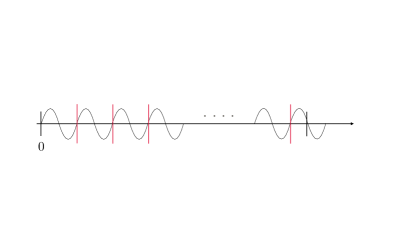
For the sake of simplicity, we focus on one day as the observational duration, where the number of the GW cycles in one day is $N_{E}\equiv[T_{E}/T_{P}]$ for the Gauss symbol $[\>]$, namely the integer part as shown by Figure 1. Note that $h(t)$ is cyclic with period $T_{P}$, while $F_{I}(t)$ has another period $T_{E}$. See Figure 2 for a daily variation of $F_{I}(t)$ for each polarization.

Figure 2: Daily variation in the antenna patterns for each GW polarization. For its simplicity, the location of the LIGO-Hanford detector and its arm direction are assumed for the sky location of the Crab pulsar.

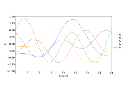
For $N$ cycles, the strain outputs can be expressed in terms of the periodic function $h_{I}(t)$ and stochastic $n(t)$. We divide the total $N$ cycles into each one cycle of $t\in[(a-1)T_{p},aT_{p})$, where $a=1,2,\cdots,N$ is an integer.

The strain output in the $a$-th cycle is denoted as $S_{a}(t)\equiv S(t+(a-1)T_{P})$ for $t\in[0,T_{p})$, which is written explicitly as

$$S_{1}(t)\equiv S(t)$$

$$= \sum_{I}F^{I}(t)h_{I}(t)+n(t),$$

$$S_{2}(t)\equiv S(t+T_{P})$$

$$= \sum_{I}F^{I}(t+T_{P})h_{I}(t+T_{P})+n(t+T_{P}),$$

$$\cdots$$

$$S_{N}(t)\equiv S(t+(N-1)T_{P})$$

$$= \sum_{I}F^{I}(t+(N-1)T_{P})h_{I}(t+(N-1)T_{P})$$

$$~{}~{}~{}~{}~{}+n(t+(N-1)T_{P}).$$ (3)

Note that $S_{a}(t)\neq S_{b}(t)$ for $a\neq b$, because $F^{I}(t)$ changes periodically with the Earth rotation but its period is not $T_{p}$ but $T_{E}$.

In order to use the least square method, therefore, let us define $A(t)$ by

$$A(t)\equiv \left(S_{1}(t)-\sum_{I}F^{I}_{1}(t)h_{I}(t)\right)^{2}$$

$$+\cdots+\left(S_{N}(t)-\sum_{I}F^{I}_{N}(t)h_{I}(t)\right)^{2}$$

$$= \sum_{a=1}^{N}\Bigl{(}S_{a}(t)-F^{I}_{a}(t)h_{I}(t)\Bigr{)}^{2},$$ (4)

where Eqs. (2) and (3) are used and $F^{I}_{a}(t)\equiv F^{I}(t+(a-1)T_{P})$. In the rest of the paper, the $N$-cycle sum $\sum\limits_{a=1}^{N}$ is abbreviated as $\sum\limits_{a}$.

In the least square method, the expected $h_{I}(t)$ at time $t$, denoted as $h_{IN}(t)$, is determined by five equations as $\partial A(t)/\partial h_{I}(t)=0$ for each $I$, where the subscript $N$ indicates the dependence on the number of cycles. Note that $h_{IN}(t)\neq h_{I}(t)$, because $h_{IN}(t)$ depends on the number of the cycles. According to the laws of large numbers in probability theory, $h_{IN}(t)$ approaches the true $h_{I}(t)$ as $N\to\infty$.

The coupled equations for $h_{IN}(t)$ are rearranged in a vectorial form as

$$M_{N}(t)\vec{H}_{N}(t)=\vec{L}_{N}(t),$$ (5)

where we define

$$\overrightarrow{H}_{N}(t) \equiv\begin{pmatrix}h_{+N}(t)\\ h_{\times N}(t)\\ h_{VN}(t)\\ h_{WN}(t)\\ h_{SN}(t)\end{pmatrix},$$ (6)

$$\overrightarrow{L}_{N}(t) \equiv\begin{pmatrix}\sum\limits_{a}F^{+}_{a}(t)S_{a}(t)\\ \sum\limits_{a}F^{\times}_{a}(t)S_{a}(t)\\ \sum\limits_{a}F^{\rm{V}}_{a}(t)S_{a}(t)\\ \sum\limits_{a}F^{\rm{W}}_{a}(t)S_{a}(t)\\ \sum\limits_{a}F^{\rm{S}}_{a}(t)S_{a}(t)\end{pmatrix},$$ (7)

$$M_{N}(t) \equiv\begin{pmatrix}\sum\limits_{a}[F^{+}_{a}(t)]^{2}&\sum\limits_{a}F^{+}_{a}(t)F^{\times}_{a}(t)&\sum\limits_{a}F^{+}_{a}(t)F^{V}_{a}(t)&\sum\limits_{a}F^{+}_{a}(t)F^{W}_{a}(t)&\sum\limits_{a}F^{+}_{a}(t)F^{S}_{a}(t)\\ \sum\limits_{a}F^{\times}_{a}(t)F^{+}_{a}(t)&\sum\limits_{a}[F^{\times}_{a}(t)]^{2}&\sum\limits_{a}F^{\times}_{a}(t)F^{V}_{a}(t)&\sum\limits_{a}F^{\times}_{a}(t)F^{W}_{a}(t)&\sum\limits_{a}F^{\times}_{a}(t)F^{S}_{a}(t)\\ \sum\limits_{a}F^{V}_{a}(t)F^{+}_{a}(t)&\sum\limits_{a}F^{V}_{a}(t)F^{\times}_{a}(t)&\sum\limits_{a}[F^{V}_{a}(t)]^{2}&\sum\limits_{a}F^{V}_{a}(t)F^{W}_{a}(t)&\sum\limits_{a}F^{V}_{a}(t)F^{S}_{a}(t)\\ \sum\limits_{a}F^{W}_{a}(t)F^{+}_{a}(t)&\sum\limits_{a}F^{W}_{a}(t)F^{\times}_{a}(t)&\sum\limits_{a}F^{W}_{a}(t)F^{V}_{a}(t)&\sum\limits_{a}[F^{W}_{a}(t)]^{2}&\sum\limits_{a}F^{W}_{a}(t)F^{S}_{a}(t)\\ \sum\limits_{a}F^{S}_{a}(t)F^{+}_{a}(t)&\sum\limits_{a}F^{S}_{a}(t)F^{\times}_{a}(t)&\sum\limits_{a}F^{S}_{a}(t)F^{V}_{a}(t)&\sum\limits_{a}F^{S}_{a}(t)F^{W}_{a}(t)&\sum\limits_{a}[F^{S}_{a}(t)]^{2}\end{pmatrix}.$$ (8)

The solution for $h_{IN}(t)$ is thus

$$\overrightarrow{H}_{N}(t)=M_{N}^{-1}(t)\overrightarrow{L}_{N}(t),$$ (9)

where $M_{N}^{-1}(t)$ is the inverse matrix of $M_{N}(t)$. $\overrightarrow{L}_{N}(t)$ in the right-hand side of Eq. (9) includes noise through $S_{a}(t)$. Thereby the reconstructed waveform of $\overrightarrow{H}_{N}(t)$ ($\neq\overrightarrow{H}(t)$) is influenced by noise.

We refer to $M_{N}(t)/N$ as the cyclically averaged antenna matrix (CAAM), because the procedure of $\frac{1}{N}\sum_{a}$ is the averaging for the $N$ cycles. One may ask if $M(t)/N$ corresponds to the covariance matrix. This is not the case, because the averaging of $F^{I}(t)$ as $\frac{1}{N}\sum_{a}F^{I}_{a}(t)$ does not always vanish.

The formal solution as Eq. (9) with Eqs. (6)-(8) shows clearly the existence and uniqueness of the solution for the inverse problem. In practical calculations, however, we do not need obtain $M^{-1}(t)$, for which numerically performing the inverse of a matrix is rather time-consuming. It is sufficient and even convenient to solve Eq. (5) by using a more sophisticated algorithm, e.g. LU (lower-upper) decomposition NumericalRecipe , which makes numerical calculations faster than the inverse matrix method.

Figure 3: Time-domain reconstruction: From $S(t)$ to $h_{I}N(t)$ by Eq. (9). The uint of the vertical axis is arbitrary. Top left: $N=1309090$, Top right: $N=2618181$, Bottom left: $N=3927272$, Bottom right: $N=5236363$, each of which corresponds to $6,12,18,24$ hours, respectively. The LIGO-Hanford detector configuration (its position and arm direction) and the Crab pulsar ($T_{p}=16.5$ msec.) are assumed, where GW waveforms follow sine functions, indicated by solid black (in color) lines. For exaggerations, the GW amplitude for the extra polarizations (S, V, W) is chosen as 0.1, and the noise $n(t)$ obeys a Gaussian distribution with the standard deviation of 20, such that the plots can be recognized by eyes. For $N=1309090$ cycles ($6$ hours), the TT modes are well reconstructed, whereas the S, V, W modes and noises are hardly distinguishable from each other by eyes. As $N$ increases, the noise is effectively reduced as $n_{eff}(t)\propto 1/\sqrt{N}$. The S, V and W modes are thus reconstructed in time domain better for $N=$5236363 (24 hours). As a simple example, an offset is considered only for $h_{S}(t)$, which may reflect the arrival time difference due to the polarization-dependent speed of gravity. The arrival time delay is chosen as $T_{p}/60$. The offset is reconstructed in the present method using Eq. (9).

Figure 4: Mock data of strain outputs for one of the $N$ cycles (16.5 msec.) in the numerical calculations for Figure 3. The standard deviation of the noise is chosen as 20, where the amplitude of TT modes is the unity. One cannot recognize the TT signal only from this plot.

Up to this point, we have assumed $\det M_{N}\neq 0$, where $\det$ denotes the determinant of a matrix. If $\det M_{N}=0$, it describes a curve in the sky, for which the CAAM is degenerate. Does $\det M_{N}=0$ occur? No, $\det M_{N}$ does not vanish. It is positive anywhere in the sky, according to numerical computations. Currently, a mathematical proof of $\det M_{N}>0$ is not obtained, because the expression of $\det M_{N}$ is very complicated.

III.2 Numerical examples

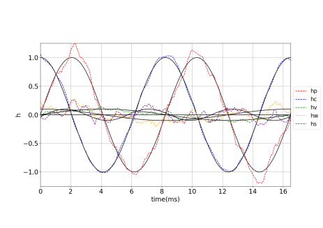
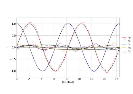
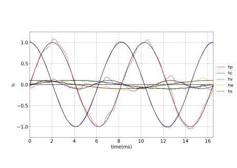
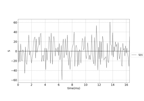
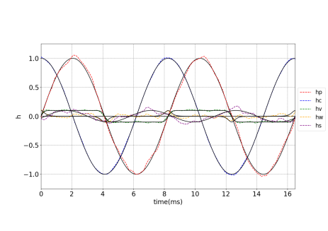
Figure 3 shows numerical time-domain reconstructions of waveforms for each polarization state, where one day observation and a pulsar GW period of 16.5 milliseconds (e.g. for the Crab pulsar) are assumed, corresponding to $N\sim 5\times 10^{6}$, because of the limited computational resources. In this figure, the amplitudes of $h_{+}(t)$ and $h_{\times}(t)$ are equal to each other, denoted simply as $h_{TT}$. $h_{S}=h_{V}=h_{W}=h_{TT}/10$ and $\bar{n}=20\times h_{TT}$ are chosen for exaggerations, such that plots can be recognized by eyes. Here, the amplitudes of $S$, $V$ and $W$ modes are denoted as $h_{S},h_{V},h_{W}$, respectively, and the standard deviation of the noise is denoted as $\bar{n}$. See Figure 4 for strain outputs during one of the $N$ cycles corresponding to Figure 3.

For $N$ cycles, the noise contribution $n(t)$ can be reduced effectively to $n_{eff}(t)\equiv\frac{1}{N}\sum_{a}n_{a}(t)\sim\bar{n}/\sqrt{N}$, when the noise obeys a Gaussian distribution, we denote $n_{a}(t)\equiv n(t+(a-1)T_{P})$ and $N$ is large. Namely, $n_{eff}(t)$ gets smaller $\propto N^{-1/2}$, as $N$ increases. In Figure 3, roughly estimating, the typical size of $n_{eff}(t)$ is $\sim n(t)/1100,n(t)/1600,n(t)/2000,n(t)/2300$, respectively, for $N\sim 1.3\times 10^{6},2.6\times 10^{6},3.9\times 10^{6},5.2\times 10^{6}$. These estimated noise contributions are consistent with Figure 3.

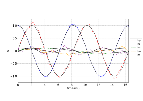
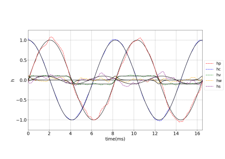
Figure 5 shows another numerical reconstruction, where non-sinusoidal waveforms are mixed. The Jacobi elliptic $sn$ and $cn$ functions are assumed for $h_{V}(t)$ and $h_{W}(t)$, respectively. By using Eq. (9), each polarization state is reconstructed from strain outputs including not only sinusoidal but also non-sinusoidal small components. .

Figure 5: Time-domain reconstruction including non-sinusoidal waveforms: The detector location with its x-arm direction and the GW source position are the same as those in Figure 3. $T_{P}$ is 16.5 msec. Top panel: $N$ is chosen as $5184000$, corresponding to nearly 24 hours. Bottom panel: $N=10368000$ (48 hours). The unit of the vertical axis is arbitrary, normalized by the amplitude of the TT modes (blue or red plots in color). The amplitude of the S, V and W modes (purple, green or yellow plots in color) and the Gaussian noise are the same as those in Figure 3. The delay of the S mode is 0.275 msec. The Jacobi elliptic functions $sn(t;k)$ and $cn(t;k)$ are assumed for $h_{V}(t)$ and $h_{W}(t)$, respectively, where the modulus $m=k^{2}$ is 0.9999999998. A sharp waveform in the Jacobi $cn$ function for W mode is reconstructed better for 48 hours than for 24 hours.

IV Future prospects and possible other effects

In this section, we briefly discuss possible other effects on the current method and result.

IV.1 Stationary Gaussian noise

First, the stationary Gaussian noise is assumed in Section III. The real noise is dependent on time. Regarding this issue, we can assume that the noise is still Gaussian but time-dependent where the standard deviation of the noise is denoted as $\sigma(t)$. For $N$ cycles, we denote $\sigma_{a}(t)\equiv\sigma(t+(a-1)T_{P})$. For regressions in such a case, Eq. (4) is modified as

$$A(t)\equiv \sum_{a=1}^{N}\frac{1}{[\sigma_{a}(t)]^{2}}\Bigl{(}S_{a}(t)-F^{I}_{a}(t)h_{I}(t)\Bigr{)}^{2}.$$ (10)

The expected waveform $\overrightarrow{H}_{N}(t)$ for the $N$ cycles is obtained in the same form as Eq. (9) but the replacement as $\sum_{a}\to\sum_{a}(1/[\sigma_{a}(t)]^{2})$ must be done in the definitions of $L_{N}(t)$ and $M_{N}(t)$ by Eqs. (7) and (8), respectively.

IV.2 Noise reduction by increased cycles

Secondly, the expected continuous GW signal is much smaller than a current detector noise. Namely, $\bar{n}\gg h_{TT}$. A large $N$ is thus required. For three months ($\sim 100$ days) and twelve years for example, the effective $n_{eff}(t)$ becomes $n(t)/23000,n(t)/150000$, respectively, where $T_{p}$ is still assumed to be 16.5 msec. From a twelve-year observation, $n_{eff}(t)$ will get much smaller $\sim 10^{-5}\times\bar{n}$.

The third-generation detectors such as the CE and ET are aiming at the detector amplitude spectral density of $\sim 2-8\times 10^{-25}\mbox{Hz}^{-1/2}$ for a range of 10-500 Hz according to their white papers CE ; ET ; CE2 . For a twelve-year observation of a pulsar with $T_{p}\sim 10$ milliseconds (corresponding to $\sim 10^{2}$ Hz), $N$ is $\sim 4\times 10^{10}$. CE and ET are thus expected to put stronger constraint on the extra polarization amplitudes than the current LIGO observations. However, the present paper is unable to estimate expected signal-to-noise ratios with the proposed formulation, because explicit waveform templates are not assumed in this paper.

IV.3 Earth rotation modulation

A third comment is related with the second one. For a very long-time observation such as three months or twelve years, a simple periodic model is not sufficient Stairs . In addition to the Earth rotation, we have to take account of the orbital motion of the Earth as well as the geophysical disturbance. These effects do not affect $h_{I}(t)$ but modify a function of time for $F^{I}(t)$. Hence, the existence and uniqueness from Eq. (9) still hold, where $M(t)$ is calculated from the accordingly modified $F^{I}(t)$. The frequency modulation due to the Doppler effect by the Earth orbital motion is stronger by nearly two orders of magnitude than that of the Earth rotation.

The Earth’s rotational speed changes mainly owing to the tidal interaction Williams ; Stephenson . The length of day (LOD) is changing at the rate of $\dot{T}_{E}\sim 2$ milliseconds per century Williams ; Stephenson , whereas giant earthquakes make the LOD longer, e.g. by 6.8 microarcseconds owing to the 2004 Indian Ocean earthquake Nature . The rate of change in the LOD, expressed as $\dot{T}_{E}/T_{E}$, is $\sim 2\>\mbox{msec.}/\mbox{day}/\mbox{century}$.

The changing LOC plays no role in $h_{I}(t)$, while it may affect calculations of $F_{a}^{I}(t)$. Therefore, we discuss how much the effect by the LOC modulation is. The change in the Earth’s spin period makes an apparent shift of both the direction of the targeted pulsar and the detector reference angle at each GW cycle.

The angle around the Earth spin axis is denoted as $\Theta(t)$. The angular velocity of the Earth is written as

$$\frac{d\Theta(t)}{dt}=\frac{2\pi}{T_{E}(t)}.$$ (11)

By taking account of the change in the LOD, this is expanded around the initial time $t=0$ as Williams ; Stephenson

$$\frac{d\Theta(t)}{dt}= \left[\frac{2\pi}{T_{E}(t)}\right]_{0}-2\pi\left[\frac{\dot{T}_{E}(t)}{(T_{E}(t))^{2}}\right]_{0}t$$

$$+O\left(\left[\frac{(\dot{T}_{E}(t))^{2}}{(T_{E}(t))^{3}}\right]_{0}t^{2}\right),$$ (12)

where the dot denotes the time derivative and the subscript $0$ denotes the value at the initial time.

By using Eq. (12), the total angle of the Earth rotation during the observation time $T_{obs}$ becomes

$$\Theta(T_{obs}) =\int_{0}^{T_{obs}}dt\frac{d\Theta(t)}{dt}$$

$$=2\pi\left[\frac{T_{obs}}{T_{E}(t)}\right]_{0}-\pi(T_{obs})^{2}\left[\frac{\dot{T}_{E}(t)}{(T_{E}(t))^{2}}\right]_{0}$$

$$+O\left((T_{obs})^{3}\left[\frac{(\dot{T}_{E}(t))^{2}}{(T_{E}(t))^{3}}\right]_{0}\right).$$ (13)

The first term in the right-hand side of the second line is the total rotation angle in the case of the constant rotation. The second term means the dominant correction due to the change in the LOD, denoted as $\Delta\Theta$. It is evaluated as

$$|\Delta\Theta(T_{obs})|\sim\> 4\times 10^{-5}\times\left(\frac{T_{obs}}{12\mbox{year}}\right)^{2}$$

$$\times\left(\frac{\dot{T}_{E}/T_{E}^{2}}{2\>\mbox{msec.}/\mbox{day}^{2}/\mbox{century}}\right),$$ (14)

which is in the unit of radians. Hence, $|\Delta\Theta(T_{obs})|$ is $\sim$ a few arcseconds.

Applying Eq. (14) to the antenna pattern function, the corresponding correction to $F^{I}_{a}(t)$ is thus $|\Delta F_{a}^{I}(T_{obs})|\sim|\partial F_{a}^{I}/\partial\theta|\times|\Delta\theta(T_{obs})|\sim O(1)\times|\Delta\Theta(T_{obs})|\sim O(10^{-5})$, where we use $\Delta\theta(T_{obs})\sim\Delta\phi(T_{obs})\sim\Delta\psi(T_{obs})\sim\Delta\Theta(T_{obs})$. Therefore, the effect due to the LOD modulation is smaller by three digits than that of the pulsar spin modulation that is estimated below as $O(10^{-2})$ for the Crab pulsar.

IV.4 Modulation of a pulsar spin period

In order to modify Eq. (9), on the other hand, we may need to take account of the modulation in the pulsar spin period Jaranowski ; Stairs , which affects both the amplitude and period of the GWs Isi2015 ; Isi2017 ; Woan .

There are several known pulsars for which the spin down rate is measured by radio observations. For the Crab pulsar for instance, its age is comparable to $\sim T_{p}/|\dot{T}_{p}|\sim 10^{3}$ years. The change $\Delta T_{p}$ in the spin period for an observational duration $T_{obs}$ is $\Delta T_{p}\sim\dot{T}_{p}T_{obs}$, which means

$$\frac{|\Delta T_{p}|}{T_{p}} \sim\left(\frac{|\dot{T}_{p}|}{T_{p}}\right)T_{obs}$$

$$\sim 10^{-2}\left(\frac{10^{3}\mbox{year}}{T_{p}/|\dot{T}_{p}|}\right)\left(\frac{T_{obs}}{12\mbox{year}}\right),$$ (15)

where we consider the Crab pulsar. The change in the pulsar spin period may not be negligible in a long-time observation. It is a few percents for twelve-year observations of the Crab pulsar.

For such a pulsar, we can estimate the spin period $T_{p}(t)$ from the form of $\dot{T}_{p}(t)=-\alpha[T_{p}(t)]^{-(n-2)}$ with a coefficient $\alpha$ and $n$ called the braking index, where $n=1\sim 3$ for most of observed isolated pulsars except for a newly born millisecond pulsar for which the GW radiation reaction term as $n=5$ is thought to be dominant for the slow down of the pulsar spin. In reality, known pulsar’s spin periods are available from radio measurements. As a practical procedure, thereby, Eq. (3) may be modified as

$$S_{1}(t) \equiv S(t),$$

$$S_{2}(t) \equiv S(t+T_{2}),$$

$$\cdots$$

$$S_{N}(t) \equiv S(t+T_{N}),$$ (16)

where we denote $T_{1}\equiv T_{p}(0)$, $T_{2}\equiv T_{p}(T_{1})$, $T_{3}\equiv T_{p}(T_{1}+T_{2}),\cdots,T_{N}\equiv T_{p}(T_{1}+\cdots T_{N-1})$ to take account of the spin period evolution as $T_{p}(t)$.

Here, let us make an order-of-magnitude estimate of the amplitude evolution Woan . We consider the GR polarization, because there are no established theories on the time evolution of non-GR polarization. In the quadrupole approximation in GR, $h_{TT}\propto T_{p}^{-2}$. Hence, we find $|\dot{h}_{TT}|\propto T_{p}^{-3}|\dot{T}_{p}|$. For the total observational time $T_{obs}$, the change in the amplitude of the GR mode is

$$\frac{|\Delta h_{TT}|}{h_{TT}} \sim\frac{|\dot{h}_{TT}|}{h_{TT}}T_{obs}$$

$$\sim\frac{|\dot{T}_{p}|}{T_{p}}T_{obs}$$

$$\sim 10^{-2}\left(\frac{10^{3}\mbox{year}}{T_{p}/|\dot{T}_{p}|}\right)\left(\frac{T_{obs}}{12\mbox{year}}\right),$$ (17)

where we use the age of the Crab pulsar $\sim T_{p}/|\dot{T}_{p}|\sim 10^{3}$ years. If non-GR amplitudes also obey a power law $h_{S}\propto T_{p}^{-\beta}$, $h_{V}\propto T_{p}^{-\gamma}$, $h_{W}\propto T_{p}^{-\gamma}$ with positive indices $\beta$ and $\gamma$, the modulation of the non-GR amplitudes follows the order-of-magnitude estimate same as Eq. (17). Namely, the total change in the amplitude for twelve-year observations is a few percents, if the slow down rate is $\sim 10^{-3}/\mbox{year}$. This suggests that the error in the reconstructed amplitude is a few percents e.g. for $\sim 12$ year observation of the Crab pulsar, when the amplitude modulation is ignored. In other words, the constant amplitude approximation in the reconstruction method is valid with $\sim$ a few percent accuracy.

On the other hand, in order to incorporate the amplitude modulation in the waveform reconstruction, specific models of non-GR modes are needed, while the amplitude evolution of TT modes can be computed by using the quadrupole formula for instance.

About pulsar glitches, radio measurements are crucial. If a pulsar glitch does not change the spin period, the current method can be applied as it is, while the data set only during the glitch may be removed in calculations for the waveform reconstruction. However, some giant pulsar glitches may make a significant change in the spin period. In this case, we have to spit the strain data stream into two sets; one data set before the glitch and the other set after the glitch. In the waveform reconstruction for the former data set, the pulsar spin period before the glitch should be used and it is given from radio measurements. For the latter data set, the spin period from radio measurement after the glitch should be used.

IV.5 Possible propagation speed test

Next, we mention the speed of extra GW modes LIGO2019 . The possible arrival time difference between the TT and extra modes does not change the current discussion, because only the GW period matters but the time translation does not affect the $N$-cycle averaging.

See Figure 3, in which the arrival time of the S-mode is different from the other modes including the GR ones. The time-domain reconstruction method allows to constrain/measure the propagation speed of the extra polarizations, if they exist, as discussed below.

Let $c_{K}$ and $c_{TT}$ denote the propagation speed of the extra polarization ($K=S,V,W$) and TT modes, respectively. We introduce a parameter $\delta_{K}$ to characterize the difference between $c_{K}$ and $c_{TT}$ by $c_{K}=c_{TT}(1+\delta_{K})$. For a pulsar at distance $d_{P}$, the arrival time difference $\Delta T_{K}$ becomes

$$\Delta T_{K}=\frac{d_{P}\delta_{K}}{c_{TT}}+O\left((\delta_{K})^{2}\right),$$ (18)

where $c_{TT}$ can be measured from a comparison of the GW speed and the light velocity for merger events such as GW170817 in multi-messenger astronomy.

By using the linearized version in $\delta_{K}$ of Eq. (18), the upper bound on $\delta_{K}$ could be placed as

$$|\delta_{K}|= \frac{c_{TT}|\Delta T_{K}|}{d_{P}}$$

$$< 1\times 10^{-15}\left(\frac{|\Delta T_{K}|}{\delta t}\right)\left(\frac{\delta t}{0.1\mbox{msec.}}\right)\left(\frac{1\mbox{kpc}}{d_{P}}\right)\left(\frac{c_{TT}}{c}\right),$$ (19)

if the arrival time difference is not detected. Here, $c_{TT}$ is almost equal to the speed of light $c$ GW170817 , a pulsar is at $d_{P}\sim 1$ kpc, the time resolution of the detector $\delta t$ limits the accuracy of measuring the arrival time difference ($|\Delta T_{K}|<\delta t$ unless the arrival time difference is detected), and $\delta t$ is assumed $\sim 0.1$ msec. This time resolution is corresponding to sampling rates $\sim 10$ kHz, which is satisfied by the current LIGO sample rate as $16$ kHz.

IV.6 Computational procedure

Before closing this section, we briefly address an issue on computational procedures and costs. We focus on the computations of Eq. (5), where we assume that the pulsar spin modulation and the Earth rotation modulation are computed somewhere else and hence the computational costs of them are not discussed here. Before we solve Eq. (5), we have to calculate $\vec{L}_{N}(t)$ and $M_{N}(t)$ that are defined by Eqs. (7) and (8), respectively. A point is that the calculations of them do not include any comparison between two different times, say 100 days or 10 years. Here, the total number of $S(t)$ and $F_{a}^{I}(t)$ equals to the total number of the data points $\sim 12\>\mbox{years}\times 16\>\mbox{kHz}\sim O(10^{12})$. for which a huge data storage is apparently required.

The present computational method is as follows. Once the strain output for the $(n+1)$-th cycle is obtained, it is added to $\overrightarrow{L}_{n}(t)$ that is the summation from the $0$-th cycle to the $n$-th one. According to the ephemeris, the values of the antenna pattern $F_{a}^{I}(t)$ are calculated for the $(n+1)$-th cycle.

As mentioned above, the present method does not make a comparison of any quantities at two different times. Therefore, we do not need a huge storage for keeping the big data of $S(t)$. Once the GW observation is done for each cycle (e.g. the $(n+1)$-th cycle), the new output data $S_{n+1}(t)$ is added to $\overrightarrow{L}_{n}(t)$ by using Eq. (7), such that we can obtain $\overrightarrow{L}_{n+1}(t)$. We continue this procedure until the $N$-th cycle, such that $\overrightarrow{L}_{N}(t)$ can be obtained.

On the other hand, the strain data is not needed when computing $M_{N}(t)$ that is the sum from $a=1$ to $a=N$. This procedure is nothing but adding the $n$-th cycle to the earlier cycles. Once $F_{a}^{I}(t)$ is evaluated at $(n+1)$-th cycle, therefore, only the new $F_{n+1}^{I}(t)$ is used for computing $F_{n+1}^{I}(t)F_{n+1}^{J}(t)$ that is added to $M_{n}(t)$ until the $N$-th cycle. Then, we obtain $M_{N}(t)$.

This additive operation is repeated until the $N$-th cycle, in which it is not necessary to keep the whole strain data and the antenna pattern values in the storage.

In this way, we obtain $\overrightarrow{L}_{N}(t)$ and $M_{N}(t)$ to arrive at Eq. (5). Eq. (5) is five linear equations for each time $t\in[0,T_{p})$, where the time step is determined by the detector sampling rate. The number of the independent linear equations is thus estimated as $T_{p}$ multiplied by the sampling rate, e.g. $\sim 16.5\>\mbox{msec.}\times 16\>\mbox{kHz}\sim 3\times 10^{2}$ for the Crab pulsar and the LIGO sampling rate. Therefore, we solve $O(10^{2})$ linear equations as Eq. (5), for which computational costs are unlikely to be extremely high as follows.

IV.7 Computing costs

Let us make a rough order-of-magnitude estimate of computing costs. In order to numerically obtain Eq. (5), we need compute numerically Eqs. (7) and (8) for $\overrightarrow{L}_{N}(t)$ and $M_{N}(t)$, respectively. The number of the GW strain data points $S_{a}(t)$ is $N$. It is $O(10^{12})$, where a data sampling rate is still assumed to be $\sim 10$ kHz for twelve-year observations. The number of computational steps in Eq. (7) is $5\times N$. This is smaller than that in Eq. (8), which defines a $5\times 5$ matrix, as $25\times N$. Hence, Eq. (8) is dominant in computational costs.

The number of computational steps for $F_{a}^{I}(t)$ for each polarization at each data point is roughly $O(100)$, because $F_{a}^{I}(t)$ is a polynomial of sine (or cosine) functions and computational steps for a sine (or cosine) function are assumed to be $O(10)-O(50)$. Hence, the total steps for computing Eq. (8) is calculated as $O(5\times 100\times 25\times N)=O(12500\times N)$, where five polarization states are still considered. This is $O(10^{16})$ for $N=O(10^{12})$ in twelve years.

The performance of a current high-speed personal computer (PC) is roughly 100 GFLOPS (giga floating point operations per second). Therefore, the computational time for obtaining Eq. (8) and hence Eq. (5) is roughly equal to $O(10^{16})$ steps divided by 100 GFLOPS. This leads to $O(10^{5})$ seconds, namely one core-day. If extra time in data transfer and so on is taken account of, the total computational time is roughly a few core-days.

V Conclusion

We considered a possible daily variation of antenna patterns for a ground-based GW detector due to Earth rotation. By defining the CAAM for continuous GWs from a known pulsar, we showed that distinct polarization states can be reconstructed in time domain from a given set of the strain outputs at a single detector.

Constraining the propagation speed of extra polarization modes, if they coexist with the TT modes, was also discussed. We have to await significant progress in computational technology before the present method can be applied also for all-sky surveys of unknown pulsars, if the pulsar GW period and sky location are included as fitting parameters.

We discussed also possible effects due to the LOD modulation as well as a secular change in the pulsar period. Numerical simulations are needed, when we wish to take account of these effects accurately. It is left for future.