Gower Street, London WC1E 6BT, United Kingdomppinstitutetext: Theoretical Particle Physics and Cosmology Group, Physics Department,
King’s College London, University of London, Strand, London WC2R 2LS, United Kingdomqqinstitutetext: LIGO Laboratory, California Institute of Technology, Pasadena, California 91125, USArrinstitutetext: Department of Physics, California Institute of Technology, Pasadena, California 91125, USAssinstitutetext: Amherst Center for Fundamental Interactions, Department of Physics,
University of Massachusetts, Amherst, MA 01003, U.S.A.ttinstitutetext: Physics Department, Swansea University, SA28PP, UKuuinstitutetext: Institute for Theoretical Particle Physics and Cosmology (TTK), RWTH Aachen University, D-52056 Aachen, Germanyvvinstitutetext: Service de Physique Théorique, Université Libre de Bruxelles, Boulevard du Triomphe, CP225, 1050 Brussels, Belgium.
Probing Anisotropies of the Stochastic Gravitational Wave Background with LISA
Abstract
We investigate the sensitivity of the Laser Interferometer Space Antenna (LISA) to the anisotropies of the Stochastic Gravitational Wave Background (SGWB). We first discuss the main astrophysical and cosmological sources of SGWB which are characterized by anisotropies in the GW energy density, and we build a Signal-to-Noise estimator to quantify the sensitivity of LISA to different multipoles. We then perform a Fisher matrix analysis of the prospects of detectability of anisotropic features with LISA for individual multipoles, focusing on a SGWB with a power-law frequency profile. We compute the noise angular spectrum taking into account the specific scan strategy of the LISA detector. We analyze the case of the kinematic dipole and quadrupole generated by Doppler boosting an isotropic SGWB. We find that is required to observe a dipolar signal with LISA. The detector response to the quadrupole has a factor relative to that of the dipole. The characterization of the anisotropies, both from a theoretical perspective and from a map-making point of view, allows us to extract information that can be used to understand the origin of the SGWB, and to discriminate among distinct superimposed SGWB sources.
1 Introduction
One of the main targets of the LISA gravitational wave (GW) detector is the detection of a stochastic gravitational wave background (SGWB), which can shed light on the physics of the early universe and on astrophysical population properties not accessible with resolved sources. There are many possible astrophysical and cosmological sources which contribute to the stochastic background (see e.g., Regimbau:2011rp ; Maggiore:2018sht ; Caprini:2018mtu for recent reviews), and up to now we have only upper bounds on its amplitude in TheLIGOScientific:2016dpb , and on parameters characterising its directional properties TheLIGOScientific:2016xzw ; KAGRA:2021mth , by the LIGO/Virgo collaboration. On the other hand we have a recent claim of a possible detection of a SGWB signal in the nano-Hertz regime by the NANOGrav collaboration Arzoumanian:2020vkk . Typically it is expected that each source is characterized by a specific spectral shape Caprini:2019pxz ; Flauger:2020qyi , however, given the plethora of sources (both resolved and unresolved) which are present in the LISA band (i.e., milli-Hertz regime), it is important to study other features which can allow for a better characterization and detection of this signal.
Interesting properties can be extracted by measuring the anisotropies in the SGWB. The first attempts for extracting information on the anisotropies of the SGWB have been first done in Allen:1996gp for the case of ground-based interferometers, in Cornish:2001hg for space-based interferometers, and in Mingarelli:2013dsa ; Taylor:2013esa for pulsar timing arrays.
The aim of this work, developed within the LISA Cosmology Working Group, is to analyze the capabilities of LISA LISA:2017pwj to detect anisotropies of the SGWB in the milli-Hertz band, making use of current instrument specifications, as well as of the latest theoretical characterizations of sources of SGWB anisotropies. The work is developed in two main parts: The first part is more theoretical in nature, and reviews our present understanding of cosmological and astrophysical sources for the SGWB and the properties of its anisotropies; The second part contains new results on the characterisation of angular response functions for LISA, accompanied by forecasts of the detectability of an anisotropic SGWB with LISA.
The theory part of our work starts with a review of a Boltzmann equation approach for analyzing anisotropies of the SGWB Contaldi:2016koz ; Bartolo:2019oiq ; Bartolo:2019yeu ; Cusin:2018avf ; Pitrou:2019rjz , similarly to what is commonly done for the Cosmic Microwave Background (CMB). This method is convenient for distinguishing effects on anisotropies sourced at the moment of GW production, from anisotropies developed as GWs propagate through our inhomogeneous universe. We then discuss early universe sources of the SGWB, and we describe SGWB anisotropies produced from inflationary mechanisms and from the formation of primordial black holes (PBH). Similarly to CMB photons, gravitons are also affected by the Sachs-Wolfe and Integrated Sachs-Wolfe effects, both related to the propagation of GW through a perturbed universe. Besides these contributions, we discuss the intrinsic SGWB anisotropy generated at the moment of production, whose frequency-dependence represents a peculiar signature of GW. We then discuss a case where GW anisotropies are induced by primordial non-Gaussianity, showing that in certain scenarios such a contribution can be relatively large. Then we study the anisotropies expected in some post-inflationary mechanisms, like preheating in a scale invariant model Bethke:2013aba ; Bethke:2013vca – even if the GW background in this model is typically peaked at larger frequencies Figueroa:2017vfa , beyond the LISA frequency band. We finally review another two main GW sources that are characterized by anisotropies: phase transitions and topological defects. For phase transitions, if only cosmological adiabatic perturbations are considered, the fluctuations in any causally produced GW background will follow those in the CMB, and hence they are expected to be small Geller:2018mwu ; Kumar:2021ffi .
For GW sourced by topological defects, anisotropies induced by a network of Nambu-Goto cosmic string loops have been computed in Jenkins:2018lvb ; Kuroyanagi:2016ugi ; Olmez:2011cg . It has been shown that while the angular power spectrum – the quantity characterising the multipole decomposition of the SGWB spectrum – depends on the model of the loop network, the anisotropies are driven by local Poisson fluctuations in the number of loops, and the resulting angular power spectrum is spectrally white (i.e., with respect to ), regardless of the particular loop distribution Jenkins:2018lvb .
We then present the case of anisotropies generated from astrophysical sources of GWs. LISA will be sensitive to several astrophysical sources such as Super Massive Binary Black Holes (SMBBHs) with masses , stellar origin Binary Black Holes (SOBBHs), Extreme Mass Ratio Inspirals (EMRIs) and Galactic white dwarf Binaries (GBs). Beyond these resolvable sources, measurements by LISA will also be affected by a huge number of unresolvable events which will sum up incoherently, forming a SGWB Farmer:2003pa ; Regimbau:2009rk ; Regimbau:2011rp . At least two SGWB components are guaranteed to be present in the LISA band: a contribution due mostly due to GB inspirals in the low-frequency band of (up to Hz), and a contribution from extra-galactic BBH mergers expected at slightly higher frequencies ( Hz). The analytic derivation of the energy density anisotropies for an SGWB has been well studied in the literature Cusin:2017fwz ; Contaldi:2016koz ; Cusin:2017mjm ; Cusin:2018avf ; Pitrou:2019rjz ; Bertacca:2019fnt . Predictions for the energy density angular power spectrum have been presented in Cusin:2018rsq ; Jenkins:2018uac ; Jenkins:2018kxc ; Cusin:2019jpv ; Cusin:2019jhg ; Bertacca:2019fnt in the Hz band and in Cusin:2019jhg in the mHz band (see Bellomo:2021mer for a recent numerical code to estimate the angular spectrum of the anisotropies of the astrophysical GWB). Anisotropies show a range of variability depending on the underlying astrophysical model for star formation, mass distribution and collapse, and on the considered cosmological perturbation effects. Due to its stochastic nature, we characterise the anisotropies in terms of their angular power spectrum taking into account all the cosmological and astrophysical dependencies.
We then move to the second part of this paper containing original results on prospects of detection of anisotropies of the SGWB with LISA, given the current instrument specifications. The characterisation of the angular resolution of space-based detectors as LISA has been pioneered in Peterseim:1997ic ; Cutler:1997ta ; Moore:1999zw , and previous studies on LISA capabilities in detecting and characterising SGWB anisotropies include Ungarelli:2001xu ; Seto:2004np ; Kudoh:2004he ; Taruya:2005yf ; Taruya:2006kqa . We start our analysis computing the angular response functions of LISA to the different multipoles for a statistically isotropic SGWB. We work in the A, E, T Time-Delay-Interferometry basis (see Tinto:2001ii ; Tinto:2002de ; Hogan:2001jn ; Tinto:2004wu ; Christensen:1992wi ; Adams:2010vc , as well as the comprehensive review Romano:2016dpx ) and we compute the angular response as a function of frequency for the auto-correlation channels (AA, EE, and TT) and cross-correlated ones (i.e. AE, AT). We also give their analytic expression in the low frequency limit. We develop an estimator for the angular power spectrum , giving a simple analytic tool to estimate the total sensitivity of LISA to an anisotropic signal. With these tools we estimate the minimal amplitude of GW energy density needed for detecting higher multipoles. As a concrete example, we analyse the case of the kinematic dipole and quadrupole generated by boosting with a factor an isotropic SGWB. We find that for one year of observation, is required to observe a dipolar signal with LISA. We also find that the detector response to the quadrupole has a factor relative to that of the dipole.
We then perform a Fisher matrix analysis aimed at forecasting the amplitude required on the lowest multipoles of the SGWB angular power spectrum for being detectable with LISA, given the current information on LISA strain and angular resolution sensitivity. We consider a power-law SGWB spectrum peaking at some multiple characterised by a fiducial amplitude and spectral tilt.
The peak in sensitivity for occurs at higher frequencies than that for . Therefore, if we choose the pivot scale of the power-law signal to coincide with the peak sensitivity frequency of the multipoles, so that their detectability is only weakly sensitive to the spectral index, we then find a greater sensitivity for in the case of a positive spectral tilt.
Finally we apply the maximum likelihood map-making method for stochastic backgrounds proposed in Contaldi:2020rht to the LISA detector, in order to provide estimates for the noise angular power spectrum . We simulate and map the noise directly in the sky domain, and we take into account the specific scan strategy of LISA, which describes how the sky signal is sampled as a function of time.
The structure of this paper is as follows: in Section 2 and 3 we review the main cosmological and astrophysical GW sources and their predicted angular power spectra; in Section 4 we present the LISA angular response function to different multipoles and the Signal-to-Noise (SNR) estimator for anisotropic signals. In Section 5 we perform a Fisher matrix analysis for the amplitude and spectral tilt of a SGWB signal characterized by a power-law behaviour. Finally in Section 6 we compute the noise angular power spectrum of LISA for different multipoles using a map-making approach. A conclusion and some technical appendices conclude the work.
2 Cosmological Sources of Anisotropies
2.1 Theoretical framework
The SGWB energy is controlled by the energy density spectrum defined as
| (1) |
with being the energy density in GW contained in the comoving momentum interval to , and corresponding to the critical energy density of the present-day universe. As we are going to discuss, we expect that the quantity is characterized by an averaged isotropic component plus a direction-dependent component. Both the isotropic and the anisotropic contributions are two key observables that can be targeted by the GW LISA detector. Several cosmological sources can produce a monopole GW energy density within the reach of the LISA sensitivity: inflationary models beyond vanilla single-field scenarios, where the inflaton is coupled with extra (gauge) fields Barnaby:2010vf ; Cook:2011hg ; Sorbo:2011rz ; Barnaby:2011qe ; Dimastrogiovanni:2016fuu ; Peloso:2016gqs ; Domcke:2016bkh to models with features in the scalar power spectrum Flauger:2009ab ; Braglia:2020eai ; Fumagalli:2020nvq , or models where space-time symmetries are broken during inflation Endlich:2013jia ; Koh:2013msa ; Cannone:2014uqa ; Cannone:2015rra ; Bartolo:2015qvr ; Ricciardone:2016lym ; Bartolo:2015qvr ; Cannone:2014uqa ; Akhshik:2014gja ; Akhshik:2014bla , or scenarios where non-attractor phases characterize the Universe evolution, Leach:2001zf ; Namjoo:2012aa ; Mylova:2018yap , or second-order scalar induced GWs which are also responsible for PBH formation Acquaviva:2002ud ; Mollerach:2003nq ; Carbone:2004iv ; Ananda:2006af ; Baumann:2007zm ; Saito:2009jt ; Garcia-Bellido:2016dkw ; Cai:2018dig ; Bartolo:2018rku ; Bartolo:2018evs ; Unal:2018yaa ; Wang:2019kaf ; Cai:2019elf ; DeLuca:2019ufz ; Inomata:2019yww ; Yuan:2019fwv ; Ozsoy:2019lyy ; Pi:2020otn ; Yuan:2020iwf ; Tasinato:2020vdk . Also post-inflationary mechanisms can generate GW signals within the reach of the LISA detector: expected signals come from first order phase transitions beyond the Standard Model of particle physics, and from the subsequent generation of topological defects, including the irreducible SGWB from any network of cosmic defects. Forecasts about the detection of the isotropic monopole contribution have been performed in previous publications of the LISA Cosmology Working group: for inflationary scenarios in Bartolo:2016ami , for phase transitions in Caprini:2015zlo ; Caprini:2019egz , and for cosmic strings in Auclair:2019wcv .
All such backgrounds are also expected to display anisotropies (direction dependence) in the GW energy density , which can be generated either at the time of their production Bethke:2013aba ; Bethke:2013vca ; Ricciardone:2017kre ; Geller:2018mwu ; Bartolo:2019zvb ; Adshead:2020bji ; Malhotra:2020ket or during their propagation in our perturbed universe Contaldi:2016koz ; Bartolo:2019oiq ; Bartolo:2019yeu ; Domcke:2020xmn . For this reason anisotropies in the SGWB energy density can be considered as a new tool to characterize and distinguish various generation mechanisms of primordial GW. At the same time, they can be considered as a probe of the evolution of cosmological perturbations.
As shown in Alba:2015cms ; Contaldi:2016koz ; Bartolo:2019oiq ; Bartolo:2019yeu , SGWB anisotropies show strong analogies with those of the Cosmic Microwave Background (CMB), at least in the geometrical optics limit Dodelson:2003ft ; Bartolo:2006cu ; Bartolo:2006fj ; DallArmi:2020dar . For this reason they can be treated using the Boltzmann equation approach, i.e., computing and evolving the equation for the gravitons distribution function in a perturbed FLRW background, analogously to what is done for CMB photons. At zeroth order in the perturbations, the isotropy and homogeneity of the background imply that the graviton distribution depends only on time and on their frequency. The gravitons propagate freely, and their physical momentum redshifts during the propagation, as CMB photons. There is however a marked difference between the graviton and the photon distribution, namely the initial population of gravitons is not expected to be thermal, as we have in mind specific production mechanisms, such as inflation Barnaby:2010vf ; Cook:2011hg , phase transitions Geller:2018mwu , or enhanced density perturbations leading to primordial black holes (PBH) Bartolo:2018evs ; Bartolo:2018rku ; Bartolo:2019zvb , occurring at energy densities much smaller to what be required for the thermalization of the produced gravitons. This induces a sort of ‘memory’ of the initial state in the distribution.
The production mechanism could occur inhomogeneously in the observed universe, in a way that correlates to the large scale perturbations. This would result in an anisotropic signal arriving on Earth. Besides this initial condition, an additional anisotropic contribution is induced by the GW propagation in our perturbed universe. Working at the linearized level in a regime of a large hierarchy between the GW (comoving) momentum and the (comoving) momentum of the large scale perturbations, the graviton propagation is affected by a Sachs-Wolfe (SW) effect, which is dominating on large scales, and by an Integrated Sachs-Wolfe (ISW), similarly to CMB photons. An important difference with respect to the CMB photons is associated with the ‘decoupling’ time of the two species: while the CMB temperature anisotropies are generated only at the last scattering surface, or afterward, the universe is instead transparent to GWs at all energies below the Planck scale. For this reason, the SGWB provides a snapshot of the universe right after inflation, and its anisotropies retain precious information about the primordial cosmological evolution.
The Boltzmann equation for the graviton distribution function , with the graviton position and its momentum, is given by
| (2) |
where is the Liouville operator, while and account, respectively, for the collision of GWs along their path, and for their emissivity from cosmological and astrophysical sources Contaldi:2016koz . In the case of a cosmological SGWB, the emissivity term can be treated as an initial condition on the GW distribution, while, as we will see in section 3, in the case of an astrophysical background it is related to the astrophysical process that generate the GW signal at various redshifts, such as the black hole merging. On the other hand, we disregard the GW collision term since it affects the distribution at higher orders in an expansion series in the gravitational strength , where is the Planck mass. We assume that our universe is well described by a perturbed FLRW metric
| (3) |
where is the scale factor as a function of the conformal time , and
scalar fluctuations, and the transverse-traceless
tensor fluctuations. We can then solve the Boltzmann equation (2), at background and linear levels. The background Boltzmann equation simply reads , and it is solved by any distribution that is function only of the comoving momentum , namely .
This implies that the physical momentum of the individual gravitons redshifts proportionally to .
At linearized level, the evolution equation for becomes Contaldi:2016koz ; Bartolo:2019oiq ; Bartolo:2019yeu
| (4) |
where is the direction of motion of the gravitons. The distribution function is related to the GW energy density by
| (5) |
where we use the spectral energy density introduced in Eq. (1), which depends also on the position where the energy density is evaluated. The suffix indicates a quantity evaluated today. We can account for a possibly anisotropic dependence by defining the quantity through
| (6) |
and then the bar quantity is defined as spatial average (over the evaluation point ) of the above quantity . With these ingredients we can introduce the density contrast
| (7) |
where the homogeneous and isotropic fractional energy density is obtained from the zeroth order distributions function .
We decompose, as for the CMB, the density contrast in spherical harmonics,
| (8) |
and, under the assumption of statistical isotropy, we define the multipole coefficients through
| (9) |
As shown in Contaldi:2016koz ; Bartolo:2019oiq ; Bartolo:2019yeu , it is useful to re-define the graviton distribution function as to simplify the first order Boltzmann equation, that now in Fourier space reads222In the CMB case .
| (10) |
where the terms on the right hand side (rhs) define the so-called source function , prime denotes a derivative with respect to conformal time, and is the cosine of the angle between and . The GW density contrast is related to the and to the background energy density fractional contribution Bartolo:2019oiq ; Bartolo:2019yeu ,
| (11) |
where we recall that is the graviton comoving momentum. Many of the cosmological GW scenarios mentioned above have a GW spectrum well described by a simple power law in frequency (i.e., ). In these cases the previous relation reduces to , where is the tensor spectral index.
The solution of the Eq. (10) can be decomposed as
| (12) |
where , , and stand for Initial, Scalar and Tensor sourced terms respectively. The scalar and tensor terms correspond to the induced anisotropies arising from the propagation of GWs in a background with large-scale perturbations, and they are therefore ubiquitous for all the cosmological (and astrophysical) sources. On the contrary, the initial term is related to the initial anisotropy contribution, and it is therefore dependent on the specific mechanism for the GW production (as we review in the next sections, it can for instance arise from large scalar-tensor-tensor or tensor-tensor-tensor primordial non-Gaussianity, or in the case of preheating).
Inserting the three terms of (12) into (11), and expanding in spherical harmonics, one obtains the Initial, Scalar, and Tensor contributions to the correlators
| (13) |
which evaluate to Bartolo:2019oiq ; Bartolo:2019yeu
| (14) |
where , , and are, respectively, the power spectrum of the initial condition term, of the scalar primordial density perturbations, and of the tensor priomordial modes with helicity Bartolo:2019oiq ; Bartolo:2019yeu . Moreover, are spherical Bessel functions, while the expressions for the scalar and tensor transfer functions are
| (15) |
where and encode the evolution of the scalar perturbations in Eq. (3) in terms of the primordial variable , namely , and . Analogously, the mode function encodes the time dependence of the tensor perturbations Bartolo:2019oiq ; Bartolo:2019yeu . As we discuss below, the spherical harmonic coefficients also have a non-vanishing three point correlation function, that can be related to the primordial bispectrum of the initial condition term and of the primordial scalar and tensor modes Bartolo:2019oiq ; Bartolo:2019yeu .
2.2 Production mechanisms
2.2.1 Inflation
Inflation, a period of accelerated expansion in the very early universe, stands as one of the main pillars of our understanding of the universe origin and evolution. Primordial quantum fluctuations, magnified by the expansion, provide the seeds for structure formation. The minimal (and observationally viable) implementation of the inflationary mechanism, comprises of a single scalar field slowly rolling down its potential, at an energy scale , where and , denote, respectively, the Planck mass and the energy scale during inflation. It is generally assumed that general relativity is the theory of gravity at this energy scale. Upon considering perturbations around a homogeneous and isotropic solution, it becomes clear that tensor fluctuations in the gravity sector, i.e. gravitational waves, are a universal prediction of inflation.
The existence of a cosmological stochastic gravitational wave background (SGWB) can be tested across a wide range of scales, from its effects on the CMB B-mode polarisation, all the way to direct detection via laser interferometers. In what follows, we shall focus on the latter possibility and clarify how anisotropies in the GW energy density, imprinted at the epoch of the SGWB generation, may directly probe inflationary dynamics.
These anisotropies, encoded in the first contribution in Eq. (12), carry the imprints from the initial conditions because the Universe is essentially transparent to GWs. This is to be compared to CMB photons for which anisotropies at the initial epoch “” are erased by the multiple collisions photons suffer prior to the recombination epoch. We stress that, interestingly, anisotropies due to initial condition are strongly model dependent and thus provide the opportunity to test and distinguish among different inflationary models. To give one example, in the case of single-field adiabatic initial conditions (and for scale-invariant primordial gravitational waves) one would get, in the language of Eq. (12):
| (16) |
where is the gravitational potential perturbation (in Poisson gauge), see Bartolo:2019oiq ; Bartolo:2019yeu ; Alba:2015cms ; Ricciardone:2021kel .
Anisotropies provide a precious handle on the particle content of the very early Universe. We would like now to single out the two necessary conditions underlying the effectiveness of anisotropies specifically as a probe of inflationary interactions: (i) naturally, a primordial GW spectrum amplitude at small scales that is well-above the sensitivity curve of laser interferometers such as LISA; (iia) a sufficiently sizeable long-short mode coupling (i.e. squeezed primordial non-Gaussianity) Dai:2013kra ; Bartolo:2019oiq ; Bartolo:2019yeu ; Bartolo:2019zvb ; Dimastrogiovanni:2021mfs , or (iib) an anisotropic background tout court Bartolo:2019oiq ; Bartolo:2019yeu .
Each of the property in (i) and (ii) are unlikely to characterize single-field slow-roll (SFSR) models of inflation. Indeed, the typical frequency profile of SFSR realisations is that of a slightly red-tilted GW spectrum, with a signal below the LISA sensitivity threshold333Noteworthy exceptions include models where an attractor phase is preceded by non-attractor evolution, see e.g. Ozsoy:2019slf .. Non-Gaussianities associated to the same SFSR paradigm are also small. Remarkably, there is a growing literature on multi-field inflationary realisations that comply with both requirements. Interesting examples of anisotropies induced by primordial non-Gaussianities include those occurring in models with light spin-2 field(s) during inflation Iacconi:2019vgc ; Iacconi:2020yxn and set-ups with a non-standard symmetry breaking patterns (see e.g. Endlich:2012pz ; Endlich:2013jia ; Celoria:2021cxq ). For examples of anisotropies engendered by an anisotropic background we refer the reader to Bartolo:2019oiq ; Bartolo:2019yeu , where the case of GWs sourced by gauge fields in axion inflation is discussed. This set-up leads to anisotropies with a significant frequency dependence, in contradistinction to what happens for CMB photons.
A general treatment of anisotropies from initial (i.e. inflationary) conditions is made possible by the Boltzmann equation and the theoretical framework expounded in section 2.1. In the remainder of this subsection, we shall describe and highlight the importance of anisotropies as a probe of primordial non-Gaussianities in the sense of (iia) defined above. We will put aside (iib) as well as assume, and later quantify, a sufficiently large primordial bispectrum so as to render the anisotropy via long-short mode coupling the leading contribution. It is convenient, before elaborating on the explicit form of non-Gaussianities-induced anisotropies, to make contact with the form they take in the context of the Boltzmann treatment. The effect of a squeezed scalar-tensor-tensor (STT) primordial bispectrum on GW anisotropies is captured by the “initial conditions” term in Eq. (12) via:
| (17) |
where underscores the specific bispectrum configuration (squeezed) under scrutiny and is a placeholder for primordial non-Gaussianity of the STT type. An analogous relation exists for anisotropies induced by TTT-type correlators, i.e. GW non-Gaussianities.
The anisotropies of the GW energy density induced by, respectively, squeezed STT and TTT non-Gaussianity, have the following form Jeong:2012df ; Dimastrogiovanni:2019bfl ; Adshead:2020bji :
| (18) |
and
| (19) |
where is the elapsed from horizon re-entry to the present for the mode , and the non-linearity parameters have been defined as
| (20) |
| (21) |
and the bispectra are understood as defined in standard fashion from the squeezed limit of the three-point function in Fourier space.
The bispectrum component that appears in Eqs. (18)-(19) is the leading physical contribution to the three-point functions. It is often the case that those bispectrum diagrams that include interactions mediated by additional (w.r.t. the single-field slow-roll case) fields give the largest contribution in terms of non-Gaussianities, squeezed or otherwise.
In order to identify the regime where non-Gaussianities provide the leading contribution to anisotropies, it suffices to report here that, schematically:
| (22) |
where is the amplitude of the primordial scalar power spectrum and is the tensor-to-scalar ratio. The regimes of interest are then, respectively, those where the conditions and hold true. It is instructive to recall, for illustrative purposes, the analytical approximation to the angular power spectrum of STT-induced anisotropies:
| (23) |
which has been obtained under the simplifying assumptions of a direction-independent, scale-invariant, as well as a scale-invariant . Note that, in the large limit, due diligence requires that one implements the constraints on the same quantities available at CMB scales.
The dependence of certain contributions to anisotropies on primordial scalar modes (as e.g. Eqs. (16) and (17) indicate), provide the intriguing opportunity of cross-correlation with CMB temperature anisotropies. Naturally the latter are also dependent on scalar perturbations, as e.g. the following expression, obtained in the Sachs-Wolfe limit, indicates Dodelson:2003ft :
| (24) |
We refer the interested reader to the literature in Adshead:2020bji ; Malhotra:2020ket ; Ricciardone:2021kel ; Braglia:2021fxn ; Dimastrogiovanni:2021mfs for a thorough treatment of the topic. We find it worthwhile to briefly mention the following notion. In the case of primordial non-Gaussianity, the effectiveness of cross-correlations as a tool to constrain the non-linearity parameter hinges on two independent aspects: the amplitude and the angular dependence of the bispectrum. For example, a quadrupolar angular dependence cross-correlated with temperature anisotropies may well be suppressed with respect to the case of a monopolar .
2.2.2 Preheating and phase transitions
In standard preheating scenarios, a daughter or ’preheat’ field is coupled to an inflaton via some interaction term involving the two fields. If the inflaton potential exhibits a monomial shape at the stages following inflation, the inflaton oscillates around the minimum of its potential after inflation, inducing a non-adiabatic time evolution in the interactive mass of the preheat field. This leads to an efficient resonant production of the daughter species Traschen:1990sw ; Kofman:1994rk ; Shtanov:1994ce ; Kofman:1997yn ; Greene:1997fu , the efficiency of which depends on the inflaton-daughter coupling, as well as on the details of the inflaton potential (see e.g. Amin:2014eta ; Figueroa:2016wxr for more recent analysis). This particle production mechanism is known as parametric resonance, and it corresponds to a non-perturbative, non-linear, and out-of-equilibrium effect. We speak about broad resonance when the choice of interaction and inflationary model leads to an excitation of the field modes within broad band(s) of momenta. In this case, a significant production of gravitational waves (GWs) takes place Khlebnikov:1997di ; Easther:2006gt ; GarciaBellido:2007af ; Dufaux:2007pt ; Figueroa:2017vfa .
In large field inflationary models, the daughter field is typically ’heavy’ during inflation, as the inflaton field takes super-Planckian amplitudes. It is possible however, to find some coupling values for which the daughter field is light during most of the inflationary era, but becomes heavy only towards the last -foldings of inflation (when the inflaton rolls down its potential towards smaller values). In this case, after inflation ends, displays amplified perturbations on super-horizon scales, just as the inflaton. At the onset of preheating, sub-horizon vacuum fluctuations serve as an initial condition for parametric resonance, but these are super-imposed over almost homogeneous values of the daughter field444Such initial values are actually constant over regions that extend beyond the Hubble radius, as they are generated by super-Hubble fluctuations. The super-Hubble scale at which varies spatially depends on the modelling, and it is determined essentially by the number of -folds during which remains light.. This is precisely the crucial ingredient for the development of anisotropies in the GW background. The value of changes at super-horizon scales according to a variance , where is the number of -folds for which is a light degree of freedom, and is the inflationary Hubble scale. Initial quantum fluctuations of the daughter field at sub-horizon scales are exponentially stimulated via parametric resonance. When non linearities become relevant in the system, i.e. when back-reacts on the inflaton , the dynamics of the sub-horizon modes are influenced by the value of within each given patch. The spatial distribution of the field , and hence of the source of the GWs, will be then different at causally disconnected regions. As a result, a different amount of GWs is produced at each super-horizon region, in correspondence with the different values of .
The anisotropies in the GW energy density spectrum from preheating have been studied in detail in the scale invariant model Bethke:2013aba ; Bethke:2013vca , chosen because of its computational convenience. GW anisotropies should be however a relatively common phenomenon arising in other preheating scenarios, as long as the appropriate conditions are met. In the mentioned scenario, the lightness of before the last -folds of inflation is guaranteed if the coupling constant is taken to be . The dynamics of preheating proceeds as usual, but the initial conditions at the onset of parametric resonance are such that at each super-horizon volume there are different values , drawn from a Gaussian distribution with variance . In practice one just needs to run simulations with free values of , simply restricted to .
Employing the ‘separate Universe’ approach, Refs. Bethke:2013aba ; Bethke:2013vca compared the peaks of the GW energy density spectrum from simulations with different initial values of , run for the choice . While the GW backgrounds were always peaked at the same frequency, as expected, the peak amplitudes of the GW spectra differed significantly. For example, in the left panel of Fig. 1 we show two GW spectra obtained for slightly different values of , and it is clearly appreciated that one amplitude is larger than the other by a factor . In other words, the actual value of influences the evolution of the sub-horizon gradients of , and hence the production of GWs. To be concrete, was observed to vary up to a factor between slightly different values of (the non-linear dynamics is actually chaotic Bond:2009xx , so small variations of can lead to a large variation of sub-horizon dynamics of the modes ). The level of anisotropy produced in the energy density of the resulting GW background is characterized by the angular power spectrum of the relative GW spectral energy-density fluctuation [c.f. Eq. (9)], which can be written as a function of the values. A general formula applicable to all scenarios characterized by a light spectator field during inflation is Bethke:2013aba ; Bethke:2013vca 555From Eqs. (31), (33) and (34) of Bethke:2013vca one can verify that the quantities entering in this relation coincide with those defined here in Eq. (9).
| (25) |
where , with the mean value over the currently observable universe. This implies that the angular power spectrum of the GW energy density anisotropy is scale invariant, i.e. characterised by a plateau at small multi-poles, , analogous to the large angular scale Sachs-Wolfe plateau for the temperature anisotropies in the CMB. In the analysed preheating scenario, the relative amplitude of the GW energy density spectrum, for a reference value of (here GeV is the Planck mass), was found to have spatial fluctuations as . For other values of the anisotropy amplitude is also similar, always at the level, see right panel of Fig. 1. For comparison, recall that the relative amplitude of the CMB temperature fluctuations is of the order of . The GW anisotropies obtained in this model are therefore very large.
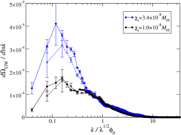
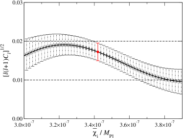
The details of the GW anisotropy, if ever observed, could provide a powerful way to differentiate between different inflationary and preheating sectors. The GW background from scale invariant preheating just discussed, is however peaked at very large frequencies Figueroa:2017vfa , way above the observational frequency window accessible to LISA (or to any other ground- or space-based planned detector for this matter). So the example mentioned only serves as a proof of principle, at least for what can be detected in the foreseeable future.
The mechanism just described corresponds to the imprint of intrinsic anisotropies in the energy density of the GW background from preheating. However, in general, other effects causing anisotropy can be also present. As a matter of fact, any causally sourced GW background will exhibit, in general, anisotropies in the spatial distribution of its energy density at large scales. This is simply due to Doppler, Sachs-Wolfe, and Integrated Sachs-Wolfe effects Contaldi:2016koz , similarly as the anisotropies arising in the photons of the CMB. This type of anisotropies concern actually not only preheating, but also GW backgrounds from cosmological phase transitions, and in general from any causally driven mechanism creating GWs after inflation (as well as inflationary GWs themselves). For cosmological adiabatic perturbations, the fluctuations in any causally produced GW background will simply follow those in the CMB, and hence they are expected to be very small Geller:2018mwu ; Kumar:2021ffi , of the order of . If primordial fluctuations carry however an isocurvature component, this need no longer be true. Ref. Kumar:2021ffi has recently shown that in non-minimal inflationary and reheating settings leading to large non-Gaussian perturbations, a non-Gaussian GW background is also expected, even when the rest of the cosmological fluids inherit predominantly Gaussian fluctuations. Primordial isocurvature perturbations can survive in the GW background say from a cosmological phase transition, exhibiting significant non-Gaussianity, while obeying observational bounds from the CMB or Large-Scale Structure surveys. Probing such inherited non-Gaussianity in causally generated GW backgrounds seems to be however a marginal possibility at LISA Kumar:2021ffi , and rather more futuristic proposals such as the detectors DECIGO or BBO are needed.
2.2.3 Topological defects
Gravitational wave sources with an inhomogeneous spatial distribution would lead to anisotropies in the SGWB, in addition to the anisotropies induced by the nature of spacetime along the line of propagation of the GWs. An inhomogeneous distribution of cosmic strings, formed generically Jeannerot:2003qv in the early Universe as a result of a phase transition, followed by a spontaneous symmetry breaking characterized by a vacuum manifold with non-contractible closed curves, will lead to anisotropies in the SGWB.
Several studies Jenkins:2018lvb ; Kuroyanagi:2016ugi ; Olmez:2011cg in the literature have calculated the anisotropies induced by a network of Nambu-Goto cosmic string loops, addressing the question of whether the model for the loop distribution will affect the angular power spectrum. It has been shown that while the amplitude of the resulting power spectrum depends on the model of the loop network, the anisotropies are driven by local Poisson fluctuations in the number of loops, and the resulting angular power spectrum is spectrally white (i.e., with respect to ), regardless of the particular loop distribution Jenkins:2018lvb .
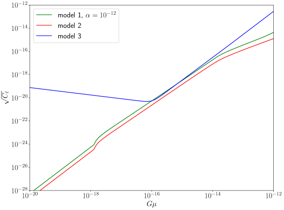
We show in Fig. 2 the amplitude of the SGWB angular power spectrum as a function of the string tension for three cosmic string loop distributions, dubbed “Model 1, 2, 3”. The first, Model 1, is the original one-scale model where all loops have the same size set by a free parameter , chosen here to be . While this model is rather obsolete, we illustrate it here since it has been shown that it leads to significant anisotropies in the PTA frequency band Kuroyanagi:2016ugi . Models 2 BlancoPillado:2011dq ; Blanco-Pillado:2013qja and 3 Ringeval:2005kr ; Lorenz:2010sm are based on different computer simulations and they differ on the way they model the production and cascade of loops from the super-horizon cosmic string network.
We find that, regardless of the adopted cosmic string loop model and the considered string tension, the predicted angular power spectrum is too small to be detected with LISA. Note that in both models 2 and 3, the monopole should be detectable by LISA for Auclair:2019wcv (though the presence of astrophysical foregrounds reduces the sensitivity somewhat to Boileau:2021gbr ).
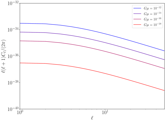
Aside from the extra-galactic population of cosmic string loops discussed above, several authors have studied the possibility of a population of loops being captured in the halo of the Milky Way Chernoff:2009tp ; Khakhaleva-Li:2020wbr ; Jain:2020dct . These loops would then give rise to an anisotropic SGWB signal which would trace the density profile of the galactic halo. Using the results from Ref. Jain:2020dct we calculate here the corresponding spectrum, which is shown in Fig. 3. Again, this signal is too weak to be detected by LISA.
2.2.4 Primordial Black Holes
In this section we review the amount of angular anisotropies inherited by the induced SGWB from primordial scalar perturbations in the scenario associated to the production of Primordial Black Holes (PBHs), see Ref. Bartolo:2019zvb for details. The standard formation scenario of PBHs requires an enhancement of curvature perturbations at small scales (denoted in this section) producing the collapse of large overdense region in the early (radiation-dominated) universe. This also predicts a copious amount of GWs induced at second order by the same scalar perturbations leading to a potential GW signature of the PBH production Acquaviva:2002ud ; Mollerach:2003nq ; Ananda:2006af ; Baumann:2007zm ; Saito:2009jt ; Garcia-Bellido:2016dkw ; Cai:2018dig ; Bartolo:2018rku ; Bartolo:2018evs ; Unal:2018yaa ; Wang:2019kaf ; Cai:2019elf ; DeLuca:2019ufz ; Inomata:2019yww ; Yuan:2019fwv ; Pi:2020otn ; Yuan:2020iwf . Since the GW emission in this mechanism mostly occurs when the corresponding perturbation scales cross the horizon, one can relate the GWs frequency to the PBHs mass as (see for example Saito:2009jt )
| (26) |
where is an efficiency factor relating the horizon scale and the PBH mass at formation epoch. Therefore, the SGWB peak frequencies fall within the LISA sensitivity band for PBH masses between around and Saito:2008jc ; Garcia-Bellido:2017aan ; Bartolo:2018rku ; Cai:2018dig ; Unal:2018yaa .
Following subsection 2.1, we adopt the following definition of the line element
| (27) |
in terms of the scalar and tensor perturbation in the Newtonian gauge, assuming no anisotropic stress. From the Einstein equation one can write down the equation of motion for the GWs as
| (28) |
where the source term on the r.h.s is evaluated assuming a radiation dominated era. The prime denotes derivative with respect to conformal time , and is the conformal Hubble parameter.
Using the equations of motion at first order in perturbation theory one can express the scalar perturbation as a function of the gauge invariant comoving curvature perturbation Lyth:1998xn . Employing the standard decomposition of the tensor perturbation in terms of the polarization tensors and helicity modes , one finds Espinosa:2018eve
| (29) |
where we have introduced the dimensionless variables and , the contracted polarization tensors , and the two oscillating functions Espinosa:2018eve ; Kohri:2018awv
| (30) | ||||
| (31) |
in terms of , with .
The energy density associated to the gravitational modes is given by Misner:1974qy ; Maggiore:1999vm ; Flanagan:2005yc
| (32) |
where the angular brackets denotes a time average on a timescale , much smaller than the cosmological timescale () but much larger than the GW phase oscillations (). Adopting the standard assumption of a Gaussian scalar curvature perturbation , one finds the fractional GW energy density
| (33) |
in terms of the critical energy density of a spatially flat universe and the curvature perturbation power spectrum .
The predicted amount of angular anisotropies can be determined by the two-point correlation function of the density field in different angular directions. For a Gaussian curvature perturbation one expects those to be undetectable, given the capability of the LISA experiment to measure anisotropies between spatial points separated by non-negligible fractions of the present horizon Bartolo:2019zvb . Indeed, according to the Equivalence Principle, the anisotropies will be highly suppressed by a factor , since the characteristic scales of the scalar perturbations are much smaller than those spatial distances, , and the emission takes place near horizon crossing.
This conclusion does not hold in the presence of primordial non-Gaussianity correlating short () and long scales (). Indeed, large scale modulation of the power spectrum may lead to anisotropies at large-scales imprinted at formation Bartolo:2019zvb . Assuming a local, scale-invariant, shape of non-Gaussianity and keeping into account propagation effects (see Sec. 2.3 for details), one can compute the two-point correlation function of the GW energy density contrast in spherical harmonics as in Eq. (9), obtaining
| (34) |
in terms of the power spectrum at large scales and the momentum dependent non-Gaussian parameter
| (35) |
Non-Gaussianity in the curvature perturbation is constrained to fall in the range at Akrami:2019izv by the Planck collaboration. It is important to stress that its presence would also generate a significant variation of the PBH abundance on large scales given the impact of long modes inducing a modulation of the power on small scales. As isocurvature modes in the DM density fluid are strongly constrained by CMB observations Akrami:2018odb , one can put an upper bound on the fraction of the Dark Matter (DM) in our universe composed by PBHs formed in the presence of non-Gaussianities Tada:2015noa ; Young:2015kda .
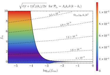
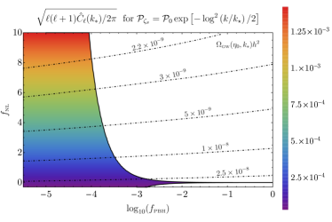
For a monochromatic and lognormal power spectra of curvature perturbations at small scales, peaked at the LISA maximum sensitivity frequency, the GW anisotropy are plotted in fig. 4, where the coloured region identifies the range of parameters allowed by the Planck constraints and the dot-dashed lines identify the present epoch GWs abundance evaluated at the peak frequency. The non-linear parameter has been assumed to be to avoid the inconsistency of the perturbative approach in the PBH abundance computation happening at larger negative values, see the related discussion in Young:2013oia ; Yoo:2019pma . The main finding is that a large fraction of DM composed by PBHs would imply a highly isotropic and Gaussian SGWB, up to propagation effects. On the other hand, the detection of a sizeable amount of anisotropy in the signal related to the PBH scenario would imply that PBHs can account only for a small fraction of the DM in the universe Bartolo:2019zvb .
2.3 Propagation effects
Independently from the initial anisotropies in the SGWB of cosmological origin, we do expect a minimal level of anisotropies in all of the scenarios described above due to the propagation of GWs through (large-scale) cosmic inhomogeneities, while travelling from the generation surface till the observation point. Such anisotropies represent an unavoidable, irreducible contribution which indeed carries precious cosmological information, being sensitive to the evolution of cosmological perturbations and to the initial conditions from which cosmic structures formed. Employing the general formalism of Boltzmann equations explained above, the underlying cosmological perturbations leave specific imprints in the statistics of the SGWB anisotropies in terms of, e.g., angular power spectra.
From Eqs. (15), we can infer some properties about the SGWB anisotropies due to their propagation through cosmological perturbations: similarly to CMB, gravitons are affected by the Sachs-Wolfe contribution, which represents the energy lost by a graviton which escapes from a potential well, and by the Integrated Sachs-Wolfe (ISW) effect, due to tensor and scalar perturbations, the latter producing an anisotropy which is roughly proportional to the total variation of the potentials . An important point to stress here is the “initial” time , which has an impact both on the SW and on the ISW contributions. The numerical evaluation of the angular power spectrum for the cosmological SGWB has been performed in DallArmi:2020dar (see also Braglia:2021fxn ), modifying the publicly available code CLASS, usually employed for the computation of CMB anisotropies Lesgourgues:2011re and adapting it to the SGWB.
In Fig. 5 we report the angular power spectrum of the cosmological SGWB due to propagation effects sourced by scalar perturbations and we compared it to the CMB one coming from temperature anisotropies. We can see that the SGWB spectrum shows a larger amplitude compared to the CMB. This can be explained considering the graviton “decoupling” time, which occurs earlier compared to CMB photons and so gravitons feel for longer time the propagation effects. In such a figure, we also report the contribution from the SW and the ISW separately, to show their behaviour at different angular scales.
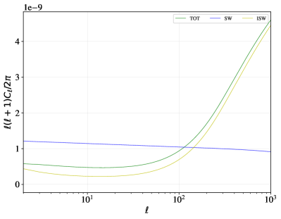
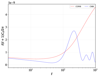
From the left plot we can see that at large angular scales (i.e., low ), the SW contribution is dominating while moving to smaller scales (i.e., ), the ISW contribution starts to be larger. On the other hand, from the right plot we can quantify the expected difference among the CMB and SGWB anisotropies.
Interestingly enough, by measuring or constraining angular anisotropies of the SGWB, it is also possible to probe the level of primordial non-Gaussianity possibly present both in the scalar and tensor cosmological perturbations through which the SGWB propagates. Indeed such primordial non-Gaussianity will left be imprinted into the GWs passing through the background large-scale underlying inhomogeneities, similarly to what happens for CMB photons. This entails to go beyond the power spectra statistics and to compute higher-order correlation functions, such as the angular bispectra of the GW energy density fluctuations Bartolo:2019oiq ; Bartolo:2019yeu
| (38) |
where is the so-called reduced bispectrum (see e.g. Komatsu:2001rj ; Gangui:1993tt ). For example, as shown in Bartolo:2019oiq ; Bartolo:2019yeu , in the case of primordial local non-Gaussianity in the curvature perturbations
| (39) |
being the linear Gaussian part of the perturbation, one finds
| (40) |
It is important to stress that similar results follow in the case of primordial non-Gaussianity in the large-scale tensor perturbations. Therefore the 3-point correlation function of GW energy density anisotropies provides for the first time a way to probe at interferometers primordial non-Gaussianity of large-scale tensor modes through the imprints that the latter leave in the spatial distribution of GW energy density as described by the second equation in (15). Indeed, for a sufficiently high SGWB, it might happen that primordial (scalar/tensor) non-Gaussianity can be measurable through the detection of the SGWB anisotropies at interferometers, even in cases where such primordial non-Gaussianity are not measurable at CMB scales.
As it is clear from the previous discussion, the seeds that give rise to anisotropies during the propagation, are the same for photons and gravitons. This naturally induces a cross-correlation among these two messengers. Recently, the cross-correlation between CMB and SGWB anisotropies induced during the propagation has been studied in Ricciardone:2021kel ; Braglia:2021fxn , and focusing on the initial anisotropy in Adshead:2020bji ; Malhotra:2020ket . All these studies have shown that such a cross correlation signal will be within the reach of the LISA detector, and it will be extremely useful to extract information on cosmological parameters, pre-recombination physics and the non-linear parameter to measure primordial non-Gaussianity.
3 Astrophysical Sources of Anisotropies
The astrophysical stochastic gravitational-wave background (AGWB) is generated by the incoherent superposition of signals emitted by a large number of resolved and unresolved astrophysical sources. In different frequency bands, several astrophysical sources can contribute to the AGWB, as merging stellar-mass black hole (SOBHB) or binary neutron stars (BNS) TheLIGOScientific:2016wyq ; Regimbau:2016ike ; Mandic:2016lcn ; Bavera:2021wmw ; Dvorkin:2016okx ; Nakazato:2016nkj ; Dvorkin:2016wac ; Evangelista:2014oba , super-massive black hole binaries (SMBHB) Kelley:2017lek , rotating neutron stars Surace:2015ppq ; Talukder:2014eba ; Lasky:2013jfa , stellar core collapse Crocker:2017agi ; Crocker:2015taa and population III binaries Kowalska:2012ba (see, e.g., Regimbau:2011rp for a review). As the cosmological GW background, also the AGWB is characterized by an isotropic energy density contribution and through the spatial angular power spectrum encoding its anisotropy.
Based on the recent observations of merging black holes and neutron star binaries by the LIGO and Virgo detectors TheVirgo:2014hva ; TheLIGOScientific:2014jea ; Abbott:2016blz ; Abbott:2016nmj ; TheLIGOScientific:2016pea ; TheLIGOScientific:2017qsa , it is estimated that the stochastic background from unresolved stellar-mass compact binaries may be detected within a few years of operation of such a network Abbott:2021xxi . Its anisotropic component is constrained by LIGO/Virgo observations up to (2019arXiv190308844T, ) which results in upper limits on the amplitude of the dimensionless energy density per units of logarithmic frequency in the range sr-1 for a population of merging binary compact objects, where denotes the angular dependence. Methods to measure and map the AGWB in the LIGO and LISA frequency ranges are discussed in Allen:1996gp ; Cornish:2001hg ; Mitra:2007mc ; Thrane:2009fp ; Romano:2015uma ; Romano:2016dpx ; Renzini:2018vkx ; TheLIGOScientific:2016xzw ; Contaldi:2020rht ; Alonso:2020mva .
Traditionally, the energy density of the AGWB has been modeled and parameterized under the assumption that both our universe and the distribution of sources are homogeneous and isotropic (see e.g. Refs. Dvorkin:2016okx ; Regimbau:2011rp ). This is a rather crude approximation: GW sources are located in galaxies embedded in the cosmic web; moreover, once a GW signal is emitted, it is deflected by the presence of massive structures, such as galaxies and compact objects. It follows that the energy flux from all astrophysical sources has a stochastic, directional dependence.
The first prediction of the AGWB angular power spectrum was presented in Cusin:2018rsq ; Jenkins:2018uac following the framework introduced in Refs. Cusin:2017mjm ; Cusin:2017fwz . This framework is flexible and splits the cosmological large-scale structure and sub-galactic scales so that it can be applied to any source contributions and any frequency band. The astrophysical dependence of the angular power spectrum on the detail of the underlying astrophysical model has been studied in Jenkins:2018kxc ; Jenkins:2018lvb ; Cusin:2019jpv ; Cusin:2019jhg ; Jenkins:2019uzp ; Jenkins:2019nks ; Wang:2021djr ; Capurri:2021zli and different formal aspects of the derivation of anisotropies and their interpretation are discussed in Contaldi:2016koz ; Cusin:2018avf ; Bertacca:2019fnt ; Pitrou:2019rjz ; Alonso:2020mva . The relative importance of cosmological and astrophysical effects depends on the frequency band chosen, hence offering the possibility to distinguish different astrophysical processes. Due to their stochastic nature, anisotropies can be statistically characterized in terms of their angular power spectrum and they also correlate with other cosmological observables such as weak lensing, galaxy number counts and CMB anisotropies.
The study of the cross correlations with electromagnetic observables provides complementary information and might improve the signal to noise of the anisotropic searches Cusin:2019jpv ; Alonso:2020mva ; Yang:2020usq ; Mukherjee:2020jxa . Moreover, cross-correlating the background that collects contribution from sources at all redshifts along the line of sight, with EM observables (such as galaxy number counts) at a given redshift, allows one to get a tomographic reconstruction of the redshift distribution of sources Cusin:2018rsq ; Alonso:2020mva ; Cusin:2019jpv ; Yang:2020usq .
3.1 GW energy density for astrophysical sources
The total present-day GW energy density per logarithmic frequency (where , see the previous section) and solid angle along the line-of-sight (note that ) of the AGWB is defined as Allen:1997ad ; Maggiore:1999vm .
| (41) |
and it represents the fractional contribution of GWs to the critical energy density of the Universe today ; is the total energy density of GWs in the frequency interval of today . See also the definition in Eq. (6). Such a quantity contains both a background (monopole) contribution in the observed frame, which is homogeneous and isotropic, i.e. , and a direction-dependent contribution .
As usual, we consider the local wave zone approximation at the source position: in other words, the observer “at the emitted position” is defined in a region with a comoving distance to the source “sufficiently large” such that the gravitational field is “weak enough” but still “local”, i.e., its wavelength is small w.r.t. the comoving distance from the observer (see also Bertacca:2017vod ; Bertacca:2019fnt ). Considering an observer that measures a GW signal in a fixed direction , one expects that the total gravitational energy density in such a direction is given by the sum of all the (unresolved) astrophysical contributions along the line of sight contained in a given volume and can be expressed as
| (42) |
from which we can build the total gravitational energy density where
| (43) |
and is related to the summation over all unresolved astrophysical sources that produce the SGWB. Here is the unit surface element at observer Cusin:2017mjm . The vector represents all the parameters which are: the halo mass , the mass of stars that give origin to the sources ; indicates the masses of the compact objects and includes the astrophysical parameters related to the model (like spin, orbital parameters, star formation rate). In Eq. (43), is the (physical) number of halos at a given mass , within the physical volume , weighted with the parameters of the sources at . The letter “” stands for “evaluated at the emission (source)” while “” for “evaluated at the observer”. Using the energy conservation we have
| (44) |
where we have redefined Here is the proper time of the observer and is the angular diameter distance. Now, defining the total GW density as
| (45) |
we can easily obtain the expression for the energy density
| (46) |
Here, are the comoving coordinates in the real frame (the “physical frame”), where is the comoving distance from the source to the detector. The previous expression depends on the position, but we can also define a position independent, isotropic version of it by integrating over a spatial volume: we denote the corresponding quantity with a bar, as in section 2.1.
We use the observer frame where we perform observations (also called “cosmic GW laboratory” in Bertacca:2017vod ). This is the correct frame where we want to reconstruct 3D maps/catalogs of galaxies by using both EM and GW signals. Let us point out that if we use unperturbed coordinates, instead of the observer coordinates, we are not able to interpret correctly the correlation between for istance the AGWB and EM sources from observed galaxies. This could induce a wrong estimate of our results Bertacca:2017vod ; Bertacca:2019fnt . In particular, we consider coordinates that are flattened in our past gravitational wave cone so that the GW geodesic from the source can be defined with the following conformal space-time coordinates
| (47) |
Here, is the conformal time today, is the comoving distance to the observed redshift and is the observed direction of the GW, i.e.
| (48) |
Using as an affine parameter in the observer’s frame, the total derivative along the past GW-cone is
| (49) |
Setting up a mapping between the observed frame and the “physical frame” in the following way , where is a suitable linear perturbation that shifts the comoving four-coordinates from the real-space frame to the observed frame. Then using the decomposition of Eq. (43), we obtain
| (50) |
with the total comoving number density at a given redshift or . Notice that, by construction, the quantity is isotropic. At linear order, we obtain the following AGWB energy density fluctuation
| (51) | |||||
where
| (52) |
and is the linear perturbation of the frequency of the GW due to the anisotropies.
Finally, let us mention that when the integration along the line of sight is performed, one should also consider the normalized selection window function , whose form depends, besides redshift, on the sensitivity/characteristics of the GW detector (see Bertacca:2019fnt and Bellomo:2021mer for more details about the window function). So we finally have
| (53) |
and
| (54) | |||||
Connection with the Halo and Stellar Mass Function and with the
Star Formation Rate
In general, the isotropic component of equation (50) is given by Phinney:2001di
| (55) |
where is the energy spectrum per unit solid angle, is the probability distribution of the source parameters and is the observed comoving merger rate density of -th unresolved type of source. In particular, the event rate (per unit of redshift) can be derived from the cosmic star formation rate. For instance, assuming for simplicity that the gravitational emission occurs shortly after the birth of the progenitor, it turns out that
| (56) |
where the term corrects the cosmic star formation rate (SFR) by the time dilation due to the cosmic expansion and is the (density) cosmic SFR in , and . Here is a generic function which depends on the initial mass function and, in general, on other parameters of the sources, as the halo mass . So then we have
| (57) |
Now, let us consider events with short emission (i.e. burst sources), as merging binary sources (BH-BH, NS-NS and/or NS-BH). Then we have
where is the merging rate of events for each halo and at a given stellar mass , and the comoving density of the halos can be rewritten as
| (58) |
i.e. the comoving density at a given . In order to give a very simple example, let us assume that and are equal for all sources. In this case they do not depend only on and we can remove the index and can be related to the fraction of mass that is bound at the epoch in halos of mass smaller than , i.e.
| (59) |
where is the comoving background density (e.g., Press & Schechter (1974) Press:1973iz , Sheth & Tormen (1999) Sheth:1999mn or Tinker (2008) Tinker:2008ff mass fraction). Following Springel:2002ux ; Hernquist:2002rg , it is possible to express the mass function in terms of the multiplicity function of halos
| (60) |
Physically, this quantity gives the fraction of mass that is bound in halos per unit logarithmic interval in mass. Finally let introduce the (mean) SFR that it is connected with in the following way
| (61) |
Note that defined in Springel:2002ux ; Hernquist:2002rg can be related to the in the following way .
3.2 Projection/propagation effects
As a first step, we compute the GW density fluctuation in the energy density in a spatially flat FLRW background in the Poisson Gauge
| (62) |
In this gauge, (where ) and the GWs overdensity is written as
| (63) |
where we have used Synchronous Comoving gauge (SC) to define the bias. In the Poisson gauge we obtain (see Bertacca:2019fnt ; Bellomo:2021mer for more details on the derivation)
where is the comoving distance at redshift , is the conformal time today, is the Hubble expansion rate in conformal time. With “” we indicate derivatives with respect to the conformal time. We have also defined the evolution bias for each source
| (65) |
Each of the four lines of Eq. (3.2) is characterized by a specific function: the gauge-invariant matter density fluctuation , the gauge invariant velocity , and the Bardeen potential . Notice that only the inclusion of all these terms allows to have a gauge-invariant observable. For a comparison and mapping between the various theoretical derivations of anisotropies presented in the literature and for a separate derivation based on a Boltzmann approach, see Ref. Pitrou:2019rjz .
3.3 Angular power spectrum for astrophysical sources
Similarly to CMB anisotropies a powerful observable to characterize the AGWB is the angular power spectrum that can be computed exploiting the spherical symmetry and working with spherical harmonics. In this section we expand the AGWB spectral energy density as
| (66) |
where the coefficients are given by
| (67) |
The AGWB angular power spectrum then reads
| (68) |
where we have defined
| (69) | |||||
where is the matter power spectrum today and are the source functions which include all the effects described in Eq. (3.2). The index refers to the specific unresolved astrophysical source while the greek index stands for the various contributions to the GW energy density anisotropies.
To have some physical insight into the information encoded in the anisotropies of the AGWB, we can use the Limber approximation. The general expression of the angular power spectrum reduces to Cusin:2017fwz
| (70) |
where is the multipole in the spherical harmonic expansion, is the galaxy power spectrum, is the (comoving) distance, related to the momentum via the Limber constraint . Each astrophysical model predicts a functional dependence of the astrophysical kernel , defined as
| (71) |
It follows that the angular power spectrum depends on the astrophysical model chosen to describe sub-galactic physics. In particular, low are sensitive to the low-redshift value of the kernel .
The angular power spectrum of the anisotropies in the AGWB from merging stellar-mass binary BHs in the mHz band where LISA operates, has been computed in Cusin:2019jhg using the astrophysical framework of PhysRevD.94.103011 . It has been shown that AGWB anisotropies are very sensitive to sub-galactic astrophysical modeling. In particular, different descriptions of stellar evolution and black hole binary formation lead to fractional differences in the angular power spectrum of anisotropies up to , independently on the global normalization (monopole) Cusin:2019jpv ; Cusin:2019jhg .
Monopole and anisotropies contain complementary astrophysical information and studying the latter will allow one to break degeneracies between different astrophysical ingredients and potentially to constrain them separately.
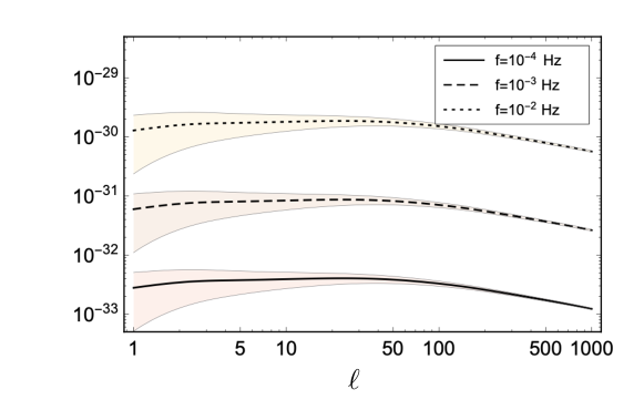
3.3.1 Systematic effects on the angular power spectrum
In estimating the anisotropies of the astrophysical gravitational-wave background, the finite number of the sources that contribute to the background at any given time and the very short time each of them spends in the frequency of the interferometer, induce a white noise (-independent) term, , in the angular power spectrum :
| (72) |
where is some direction-independent (due to statistical isotropy) function describing the variance, is the Hubble radius and stands for the angular power of the intrinsic, astrophysical anisotropy. The shot noise dominates over the true astrophysical power spectrum; the latter may be recovered with long enough observing runs and sufficient removal of a large number of foreground sources Jenkins:2019uzp .
To calculate the true, astrophysical angular power spectrum of a statistically-isotropic gravitational-wave background, a novel method, based on combining statistically-independent data segments, was proposed in Jenkins:2019nks . The proposed estimator, constructed from the cross-correlations between statistically-independent time intervals, reads
| (73) |
where (with the total observing time) denotes the number of segments and
| (74) |
The estimator (73) is unbiased since
| (75) |
where the subscripts stand for performing first the cosmological and the the shot noise average. In the limit of many data segments, , the estimator (73) has the lowest-variance
| (76) |
and, in this sense, it is the most efficient one. It is worth noting that the term in the above equation is the same as the one appearing in the mean of the standard estimator , hence (73) is still affected by the shot noise. However, now the shot noise only adds to the variance of the estimator and it does not affect the angular power spectrum, as in the standard case.
Since the shot noise power may exceed the real astrophysical angular power spectrum by a factor as high as approximately , according Jenkins:2019uzp , the proposed method for estimating the true, astrophysical angular power spectrum of a statistically-isotropic astrophysical gravitational-wave background, is indeed a valuable tool.
Another interesting method to alleviate this shot noise problem and extract information on the underlying GW population, is to make use of the cross-correlation of the AGWB background map with other cosmological observables such as galaxy distribution, see e.g. Alonso:2020mva . Indeed, the shot noise level of the cross-spectrum is primarily driven by the density of the much denser galaxy survey (although the GW shot noise will still be a significant contribution to the signal to noise of the cross-correlation).
4 LISA Angular Sensitivity
In this section we discuss the sensitivity of LISA to the anisotropies of the SGWB.
4.1 LISA angular response functions
We follow the notation of ref. Flauger:2020qyi , that we generalize to an anisotropic SGWB. We start from
| (77) |
where in the chiral basis ( denoting, respectively, the right and the left polarization), the polarization operators obey and they are normalized according to , and where reality of the mode function is ensured by . An unpolarized and anisotropic SGWB is characterized by the intensity , defined through
| (78) |
where , and are the standard spherical harmonics, with this normalization .
We want to relate the coefficients to those of the fractional energy density in the decomposition (12). Starting from Eq. (77) and from the intensity function defined in (78), we arrive to the following expression for the SGWB energy density over the critical energy density
where is the Newton constant, while the present Hubble rate. Recalling the normalization of the polarization operators, we then find
| (80) |
Proceeding as in Section 2.1, we then arrive to
| (81) |
Let us now discuss how to measure these coefficients. We consider two locations , at the unperturbed distance (by “unperturbed”, we mean the quantity in absence of the SGWB), and a photon that, starting from at the unperturbed time , arrives at at the unperturbed time . The SGWB modifies the time of flight to , with
| (82) |
where is the unit vector going from to . This time delay has an associated Doppler frequency shift Flauger:2020qyi
| (83) |
We denote by
| (84) |
the frequency shift for the closed path. Differences between closed path shifts originate the Time Delay Interferometry (TDI) 1.0 and 1.5 typically considered for LISA Flauger:2020qyi . Specifically, the TDI 1.0 combination is given by the difference between the and the path:
| (85) |
while the TDI 1.5 combination is given by the difference between the and the path:
| (86) | |||||
To simplify the notation, we denote 666Namely the index coincides with , and the index coincides with . by the i-th satellite of the LISA triangle, and define
| (87) |
We are interested in correlators between different measurements. The only statistical variable that participates non trivially in the correlator is the GW mode function, see Eq. (78). Starting from the expression in Eq. (147) for the TDI measurement, we obtain
| (88) | |||||
where the frequency is related to the LISA arm length by
| (89) |
where
| (90) |
We introduced the anisotropic LISA response function
| (91) |
with the functions are given in Eq. (148). In the isotropic case, the response function in Eq. (91) agrees with Eq. (A.21) of Flauger:2020qyi .
As we show in Appendix A, under a rigid rotation of the instrument the response function transforms as a spherical harmonic. Specifically, if is a rotation under which the position of the three satellites changes according to , we have
| (92) |
where are the elements of the Wigner -matrix. For a rotation of an angle about the axis we then have
| (93) |
Using this fact, and the property
| (94) |
(that we also prove in Appendix A), we then learn that, if we place the three satellites in the plane, the various components of the response function satisfy
| (101) |
4.2 -dependent response functions in the A, E, T channels
As shown by Eq. (92), the anisotropic LISA response functions transform as spherical harmonics under rotations. One can therefore consider the dependent response function
| (105) |
that is invariant under rotations, and therefore constant in time (it does not depend on the orientation of the LISA triangle). As we show in the next subsection, it provides an estimate for the response of LISA to a statistically isotropic SGWB, see Subsection 4.4. From the properties in Eq. (101) we learn that
| (106) |
It is customary to consider linear combinations of the measurements considered so far
| (107) |
which we write more compactly as
| (108) |
These combinations (that we have normalized as in ref. Flauger:2020qyi , so that the rotation matrix associated with these transformations is orthogonal) diagonalize the noise variance, in the hypothesis that LISA is an equilateral triangle, with identical instruments at the vertices. In terms of the channels the response function formally reads
| (109) |
We evaluate these linear combinations, accounting for the identities in Eq. (101), namely
| (110) |
The resulting expressions acquire different forms for even and odd multipoles. Specifically, for odd we find
| (111) | |||||
and for even
| (112) |
We also note that the property in Eq. (94) implies that the response fuction is symmetric in the channels, .
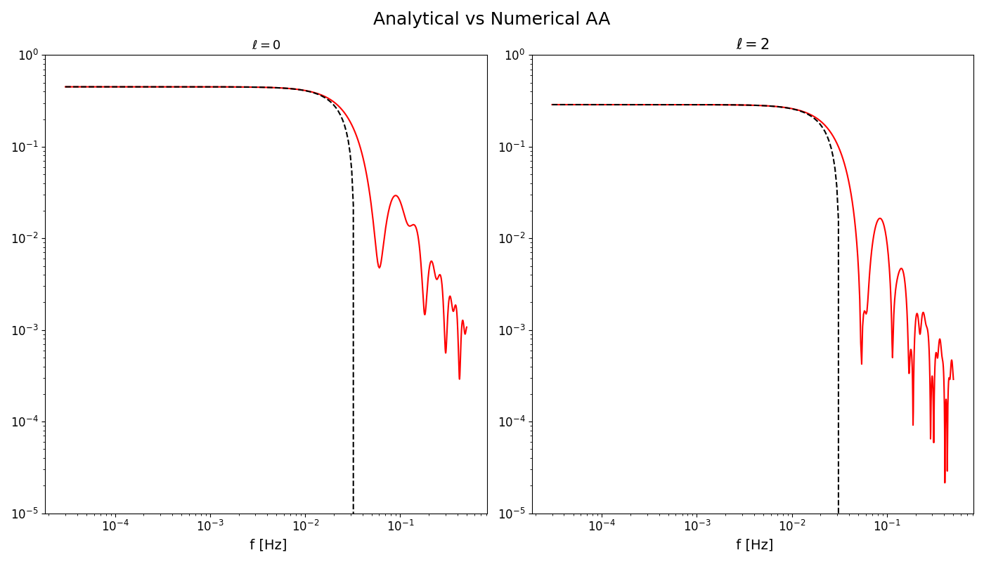
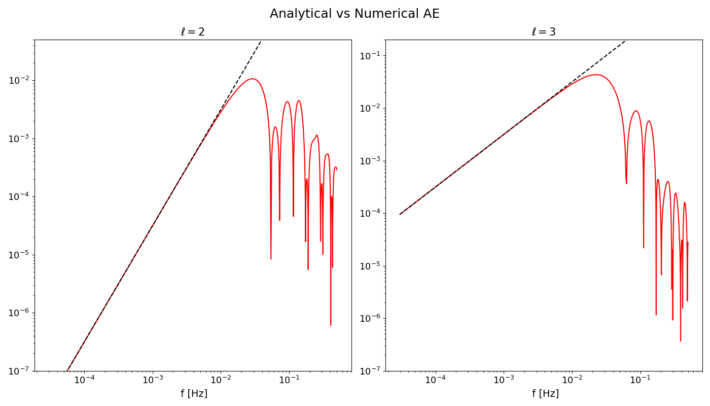
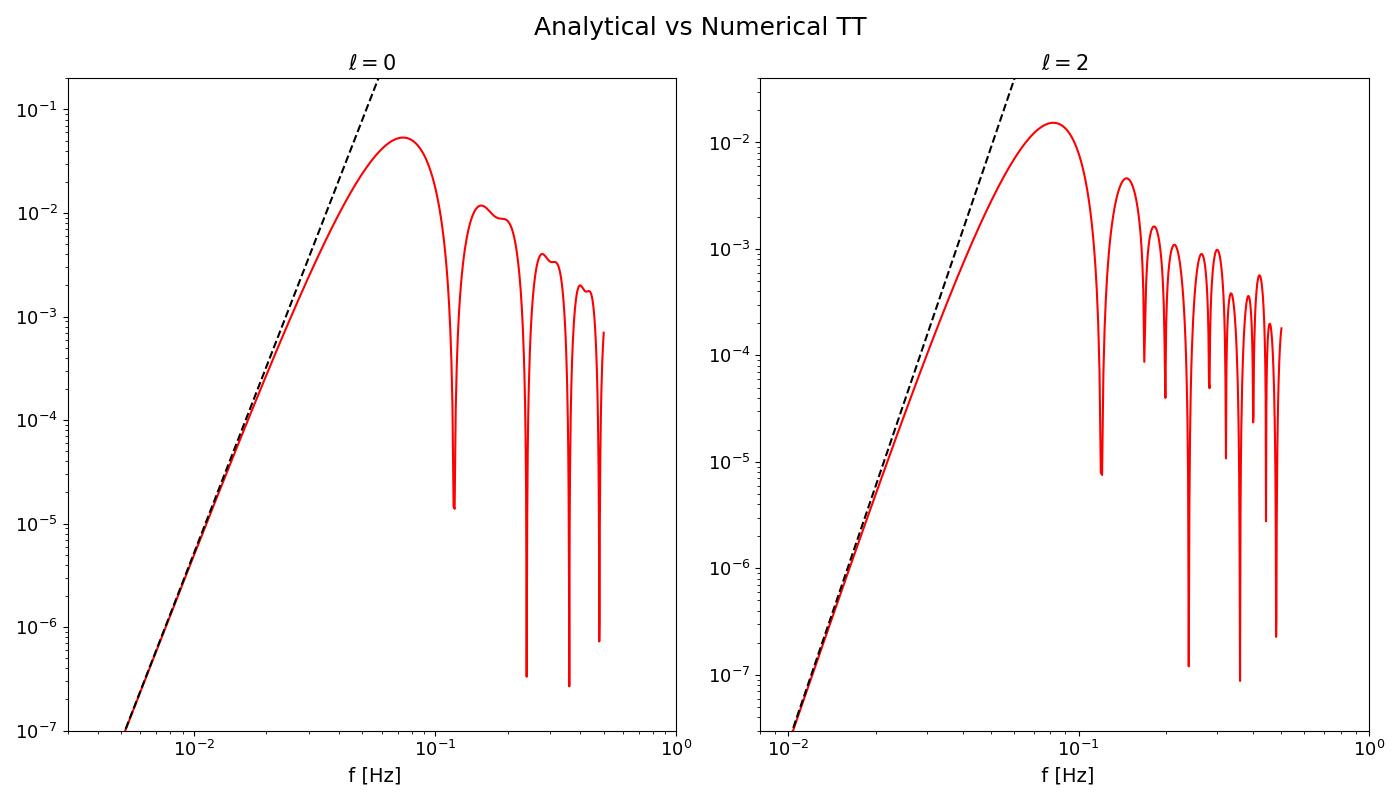
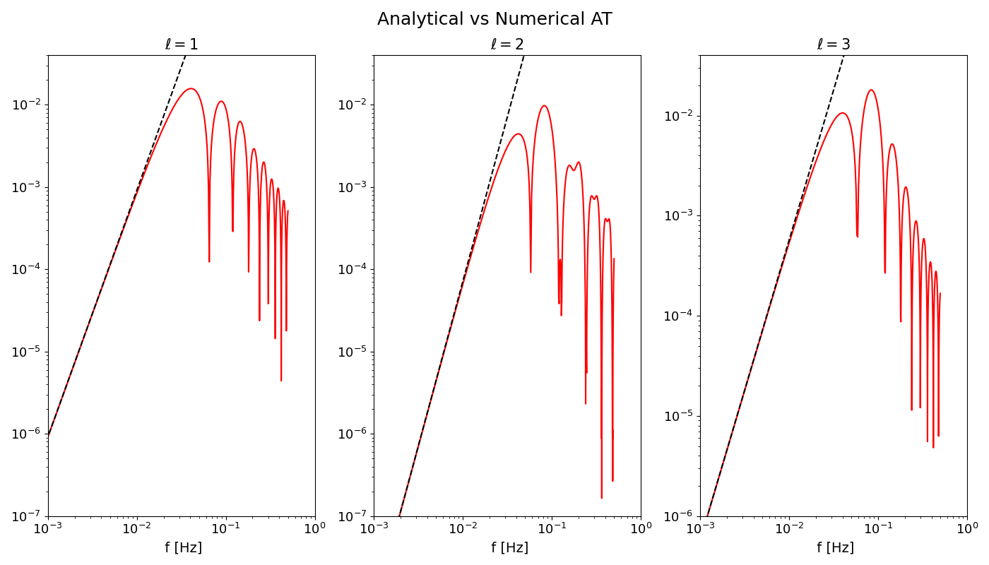
These expressions can be evaluated numerically, for arbitary frequency, or evaluated analytically in the small frequency regime. For the first few multipoles, we obtain the values in the Table 1. In Figures 7 and 8 we show instead a comparison between the full shape of the response functions and the small frequency expressions for these first multipoles.
| 0 | 0 | 0 | ||
| 1 | 0 | 0 | 0 | |
| 2 | ||||
| 3 | 0 | 0 | ||
| 4 | ||||
| 5 | 0 | 0 | ||
| 6 |
4.3 Signal-to-Noise Ratio for anisotropic signals
We consider the Fourier transform of the signal in Eq. (108), performed with an integration time
| (113) |
This signal, if present, adds up with the instrumental noise in the measurement
| (114) |
We assume that the noise is Gaussian and we recall that it is diagonal in the A,E,T basis, namely
| (115) |
where the explicit expressions for are given in Appendix B. Then we define the estimator as
| (116) |
where the functions are weights to be chosen in order to maximize the Signal-to-Noise Ratio (SNR) for this measurement Smith:2019wny . The measurement time is denoted by . For simplicity, we are integrating over equal times, disregarding correlations between measurements done at different times. In the estimator, we subtracted the expectation value of the instrumental noise associated with the measurement , so to obtain an unbiased characterization of the SGWB. From the estimator, we get the SNR
| (117) |
that, as we will see, can be made real by an appropriate choice of the weights .
As we show in Appendix B, the expectation value of the estimator is
| (118) |
where we recall that the intensity multipoles coefficients have been defined in Eq. (78), while, .
In Appendix B we also show that, under the hypothesis that the noise dominates over the signal,
| (119) |
4.4 Sensitivity to multipoles
Eq. (LABEL:SNR-ell-m) provides the SNR for the detection of a SGWB which is the sum of all possible multipoles contributions. Although we have not explicitly written it, the response functions also depend on time, as they are functions of the positions of the satellites. A full analysis of the separate contributions of the various multipoles would then require a component separation, which is in practice the inversion of the time-dependent streams measured by the satellite to the multipole amplitudes . We leave this discussion to section 6. Here we estimate the relative sensitivity of LISA to different multipoles by assuming that only one multipole dominates the SGWB and that multipoles with the same but different are obtained from the same Gaussian statistics. This amounts to assuming a statistically isotropic SGWB, with correlators given by Eq. (9).
Taking this into account, the expected SNR (LABEL:SNR-ell-m) can be written as a sum over the various multipoles,
| (121) |
where, for each multipole,
| (122) |
where we recall that the response function is the quantity defined in Eq. (110) and rescaled as in Eq. (88). In the following, we can work directly in terms of by rescaling the noise functions accordingly, see Eqs. (170) and (171). Moreover, ad discussed above, the response function to a statistically isotropic signal is time-independent, so that the integral over time in Eq. (122) simply results in the usual property that the SNR grows with the square root of the observation time. Finally, we factor out the uncertainty in the Hubble rate by dividing it by its rescaled value and by considering the combination, as it is standard. This leads to
| (123) |
From this expression we define the “channel-channel” sensitivity
| (124) |
as well as the optimally weighted sum over the three channels
| (125) |
The total sensitivity to the multiple is shown in Figure 9 for multipoles up to . From this quantity, we can immediately obtain
| (126) |
We note that the curves shown in Figure 9 are rescaled by , in such a way that the curve shown for coincides with the SciRD (Science Requirement Document) sensitivity curve for a homogeneous signal Babak:2021mhe obtained from summing over the channels.
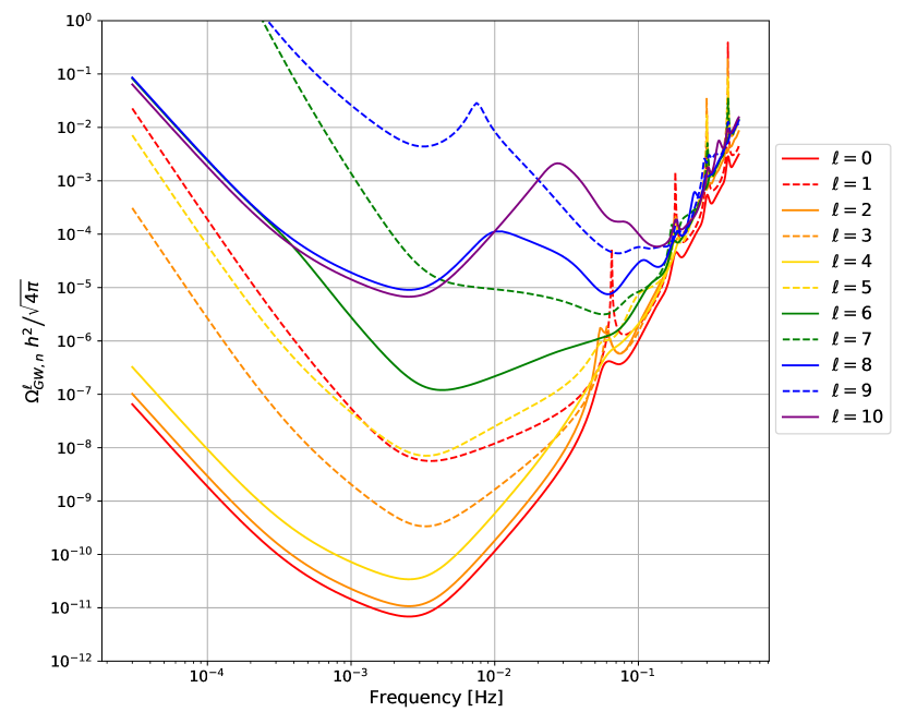
4.5 Sensitivity to kinematic anisotropies
Doppler anisotropies induced by the motion of the detector with respect to the SGWB rest frame count among the guaranteed features of the SGWB. In fact, already the early work Allen:1996gp , which sets the basis for the analysis of SGWB anisotropies with ground-based GW interferometers, estimated the prospects for ground-based detectors to measure the kinematic dipole of the SGWB. In this subsection we briefly consider the same question in the context of LISA.
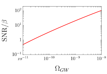
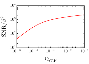
The size and properties of kinematic anisotropies depend on the frequency profile of the rest-frame SGWB energy density . This fact can be important for enhancing the amplitude of kinematic anistropies in certain early-universe scenarios where the SGWB has rich features, as the ones discussed in Section 2.
We consider two cosmological frames: the first, denoted with , is comoving with the SGWB rest frame; the second, denoted with , moves with constant velocity with respect to the rest frame . We assume that the SGWB density parameter in the rest frame, , is perfectly isotropic and depends only on frequency . A boost transformation relates the SGWB density parameter in the rest frame to the one in the moving one . We indicate with (where in units with ) the velocity of the frame with respect to the rest frame .
In the technical appendix C we derive the resulting expression of an anisotropic SGWB energy density as a function of the rest-frame density . Assuming that the parameter is small, we can Taylor expand up to second order in and write
| (127) |
The functions of frequency , , , control respectively the contributions of kinematic effects to the monopole, dipole, and quadrupole of GW energy density in the detector frame. They read
| (128) | |||||
| (129) | |||||
| (130) |
In analogy with CMB literature, we introduce the SGWB spectral tilts
| (131) | |||||
| (132) |
The expressions (128), (129), (130) quantitatively demonstrate that enhanced spectral tilts can amplify kinematic anisotropies in certain scenarios.
We plot in Figure 10 the SNR for LISA to detect the kinematic dipole and quadrupole induced by a scale-invariant profile of constant in the SGWB rest frame. Notice the different vertical scale in the two plots, due to the fact that LISA sensitivity to the quadrupole is a factor better than that to the dipole, as discussed in the previous sections.
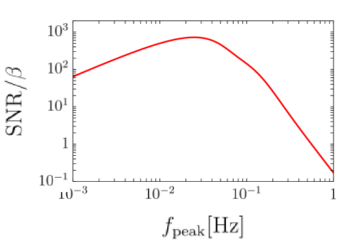
We also show in Figure 11 the sensitivity to the dipole induced by a boost with velocity on the SGWB spectrum generated by a strongly first order phase transition. We model the spectral density as a broken power law, using Eq. (8) of Ref. Caprini:2019egz , and illustrated in Fig. 3 therein. We allow the location of the break to vary, but fix the amplitude so that the total energy density integrated over all frequencies contributes of the critical energy density during the radiation era. The SNR scales linearly with the amplitude, so boosting to raises the SNR by 10. In this case, the rich frequency profile of the SGWB energy density in the rest frame leads to a pronounced frequency-dependence of the amplitude of the SNR in the LISA band.
5 Fisher Forecast
The next step of our analysis is to estimate, for the LISA strain and angular resolution sensitivity, statistical forecasts on the detectability of the lowest multipoles of the SGWB angular power spectrum, using a Fisher matrix method.
We consider a total observation time of years (corresponding to the total 4 years nominal mission assuming 75% efficiency), and a frequency resolution Hz, which corresponds to segmenting the TDI data stream into chunks of 11.5 days (i.e. the inverse of the frequency resolution), and using as the final spectrum the average over the spectra of the chunks.
We work under the assumption of statistical isotropy, where different multipoles are uncorrelated and all orders are drawn from the same distribution for each multipole (only under this assumption it is justified to average over different parts of the sky, or in practice different time segments). We consider each multipole separately, in order to obtain a measure of the information contained in each of them. In practice, when trying to recover the angular power spectrum from a sky map, different multipoles become correlated, which would degrade the results obtained here.
Following the result obtained in Eq. (126), we define the SGWB power spectrum at multipole as
| (133) |
where is the angular power spectrum of the GW density contrast as defined in Eq. (9).
For the sake of generality, we consider a power-law SGWB spectrum peaking at a fiducial multiple only, parameterized by the logarithmic amplitude at a pivot frequency Hz, that is chosen close to the frequency where LISA has the best sensitivity, and by a spectral index ,
| (134) |
For each multipole and channel combination , we assume a Gaussian likelihood over the averaged data given by
| (135) |
where is the number of data segments in the analysis; the sum runs over frequencies (or frequency bins) , denotes the averaged signal over the data segments in the channel combination , and is the theoretical ansatz for the data,
| (136) |
where is the frequency response of the detector and is the noise as defined in the previous section expressed in Omega units. The variance can be expressed in terms of the theoretical ansatz as . In practice, instead of summing over channels in the likelihood, we consider a single data vector and compare it with the effective noise combination defined by Eq. (125) and shown in figure 9, and drop the channel indices in what follows.
Assuming a fixed noise model, the Fisher information matrix for the likelihood defined in Eq. (135) is simply
| (137) |
where are a combination of the signal model parameters and , and the corresponding partial derivatives are
| (138) |
The estimated LISA sensitivity to a single-monopole power-law SGWB defined in Eq. (134) has been represented on Figure 12 for the monopole (), dipole () and quadrupole (), for a series of fiducial values of the SGWB amplitude and spectral index . In all cases, the standard deviation for each parameter is considered marginalised over the other one (i.e. taken from the diagonal elements of the covariance matrix , defined as the inverse of the Fisher information matrix).
As one can see in Figure 12, for , sufficiently high log-amplitudes are recovered independently of the sign of the spectral index (but enhanced by stronger indices), due to the pivot frequency being chosen to approximately coincide with the peak in sensitivity at both multipoles. In contrast, for positive spectral indices enhance the recovery of the amplitude. This is on the one hand because the corresponding sensitivity peaks at slightly larger frequency with respect to ; and on the other hand because of the milder slope of the sensitivity with respect to towards high frequencies, so that the power law is closer to the high-frequency noise spectrum for lower in than in (see figure 9).
For all multipoles, the spectral index is obviously recovered more effectively for higher log-amplitudes. In the optimal case of a signal amplitude of order , a null spectral index could be reconstructed with an uncertainty of order for the multipoles respectively. In the more pessimistic case of , for the spectral index could be reconstructed with an uncertainty of order or greater for largely positive or negative values of it, but this uncertainty approaches order one for SGWB spectra with a spectral index between and . In such a low-amplitude scenario, LISA will thus be more sensitive to models with a strongly varying SGWB spectrum. Notice how, for the same reasons described in the previous paragraph, the dipole is more sensitive towards positive spectral indices, whereas for the accuracy is almost symmetric with respect to the sign.
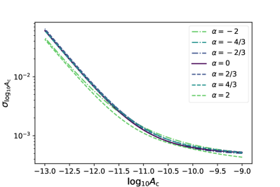
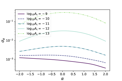
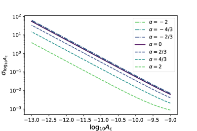
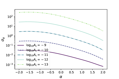
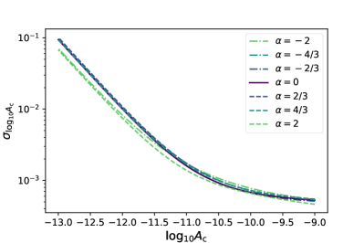
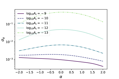
6 Map-making Method
In this section we briefly describe the maximum likelihood map-making method for stochastic backgrounds proposed in Contaldi:2020rht and provide estimates for the noise power spectrum obtained by simulating and mapping the noise directly in the sky domain. Recently, another method to map the gravitational-wave sky with LISA has been developed and it is based on a Bayesian algorithm to map the power of the SGWB using a spherical harmonic approach Banagiri:2021ovv .
The maximum likelihood map-making with GW detectors relies on the specific scan strategy of the interferometer array, which describes how the sky signal is sampled as a function of time. The reconstruction of the GW sky and the angular resolution at which it may be achieved then depend on the amount of modes sampled throughout the whole duration of the observation.
To simplify the mapping procedure we assume that the anisotropic SGWB signal intensity has a simple power-law spectral shape which may be factored out, such that
| (139) |
where , and is a specific reference frequency.
As for the scan strategy, we assume the spacecrafts follow three heliocentric, quasi-circular orbits remaining at a constant arm-length distance from each other, and that the noise in the detector is well understood. Specifically, as in Section 4, the noise is modelled by two contributions: acceleration noise and interferometer noise. For more details, see Equations (30) and (31) in Contaldi:2020rht and the description of the noise parameters in the official mock data release Sangria .
The data vector is defined (similarly to Equation (114)) as , where the first term specifies the pure signal component, made up of the contraction between the linear detector response R (see Equation 148 in the appendix) and the SGWB strain , and n is the noise component. We keep the formalism general here for the sake of conciseness; note that for multiple LISA TDI channels d is a vector in TDI space. To estimate the intensity directly, the data are considered in frequency space: with belonging to the appropriate frequency interval observed by LISA. We assume the noise is zero–mean and Gaussian with covariance and the signal component is also Gaussian such that the total, signal plus noise, covariance of the data is . Here A is the operator that describes the response of the detector to the strain intensity. This can be integrated in time and projected onto pixel or spherical harmonic space. In the case of multiple TDI channels it represents the full correlated response matrix. Also note that in the case of multiple correlated TDI channels, e.g. , , and as considered in Contaldi:2020rht , the noise covariance is the full correlated covariance matrix with the auto-correlated noise model for the diagonal and cross-correlated model for the off-diagonal terms. is the observed realisation of GWB intensity on the sky. The likelihood of the data is then
| (140) |
as described in Bond:1998zw for the case of CMB mapping, it is possible to find the iterative solution which maximises ,
| (141) | ||||
| (142) |
where is the Fisher information matrix and . In practical applications, given the constraints on scan strategies and response functions for gravitational wave observations, the Fisher matrix will need to be regularised in order the correct iterative solution to be found using Eq. (141). Here, the intensity of the sky-map is indexed generically by such that are the set of “parameters”, on which the signal component of C depends, that have to be estimated. For any particular application, the indices could stand for either map domain pixels “” or spherical harmonic domain multipoles “”. The choice here is to work in the map domain, as it is not overly expensive in this case, and leads to a clearer understanding and regularisation of the Fisher matrix, as explained in Renzini2018 ; Contaldi:2020rht ; in the latter, tests of the method and a regularisation technique are presented. In principle, the could be estimated for a frequency band as narrow as the resolution permits, however this would result in a poorly regularised problem. To improve this the estimation must be done using wider frequency bands. Here we simply adopt the broad-band limit by assuming a spectral shape as in Eq. (139). In practice this means the traces in Eqs. (141, 142) include a sum over the full frequency response, such that the final estimate is given with respect to a single reference frequency .
Note that the term represents the directional quadratic response of the detector, and is equal to up to appropriate normalisation factors. will, in general be time dependent, presenting a sky modulation with period of one year. Hence, to apply this mapping algorithm effectively, the data must be segmented into short observation time-frames, throughout which the sky response is assumed to be constant and for which the noise can be estimated accurately. The duration of each segment also sets the lower bound on the observable frequency window, hence there is a trade-off between frequency and (potential) sky resolution: in principle a shorter time window will allow access to higher pixel resolution, but it will also fix the frequency resolution to . Assuming statistical independence between time-frames, the two traces in Eqs. (141, 142) are then obtained by averaging777For actual data this average would be weighted by noise estimates but here we assume the noise is constant and uncorrelated between time-frames. over all the frames available.
For the purpose of this paper, we use the method described above directly in pixel space to calculate the noise power spectrum , assuming the LISA noise curves as in Contaldi:2020rht , over an observation time of one year. This is simply done by running the iterative map-maker over a noise-dominated data set, such that the Fisher matrix – setting now – reduces to
| (143) |
The statistically isotropised, angular power spectrum of the noise can then be estimated by expanding and inverting the Fisher matrix Renzini2019b :
| (144) |
where the linear operator and similar for its adjoint. This is similar in spirit to what is presented in Alonso2020 , however note that here the estimate is obtained by simulating and integrating the full scan strategy, without assuming the noise is isotropic to begin with. The estimates are shown in Figure 13, in units of at reference frequency Hz for a quicker comparison with signal models. This matches the convention chosen in Alonso2020 , and the mode of the two estimated noise power spectra matches well. Note that in Figure 13 an observation time of four years is assumed.
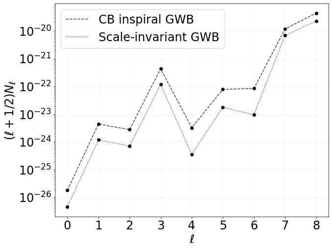
The discrepancy at odd s between the noise power spectrum obtained by the inverse Fisher matrix and the analytic computation presented in Alonso2020 is in part due to the substantially different sampling of the modes. While these are marginalised over at a fixed time in Equation (110) to obtain the instantaneous –mode response, in the map–making procedure these are kept into account, and through the scan strategy contribute to breaking the degeneracies in the odd –modes of (instantaneous) . The higher- section of the curve is highly dominated by the conditioned inversion; in fact, the noise covariance matrix found in this case is highly singular, and 90% of its eigenvalues has been discarded to produce the curve in Figure 13. The conditioning has a stronger impact on the higher- end of the angular spectrum, as the response of the detector is weaker at higher angular scales. It is therefore difficult to compare numerical estimates of the effective noise at different angular scales to the result of analytical estimates. This is an active field of research, and it is clear that a robust regularisation scheme will be required when attempting to reconstruct the higher modes of the angular power spectrum with this configuration of the LISA instrument. Inevitably, the presence of complicating factors such as non-stationarity, noise uncertainties, and scanning systematics in real data will exacerbate this issue and mapping techniques will require significant developments in order to reconstruct anisotropies as optimally as possible.
7 Conclusions
The anisotropies of the SGWB represent a powerful tool to characterize and distinguish the different sources of GWs. We have seen in this paper how different GW sources are characterized by different angular spectra. Such anisotropies have mainly two contributions: one directly related to the production mechanism of each particular GW source, and one being an effect of the propagation of GWs on our perturbed Universe, which is common for all the GWs sources. We have made an overview of the main cosmological and astrophysical sources characterized by anisotropies, that are expected to be present in the LISA frequency band. We have presented the angular spectrum for different cosmological backgrounds (i.e., inflation, phase transition, PBH and cosmic strings) and an astrophysical one (Solar Mass Black Hole Binaries). We have then built a SNR estimator to quantify the sensitivity of LISA to different multipoles. To do this, we have computed the responses of LISA in harmonic space as functions of frequency for the AET TDI channels. We have also derived the analytic form of the responses in the low frequency limit. It is important to stress that, when anisotropic signals are considered, both the auto-correlation responses (i.e., AA, EE) and cross-correlation ones (i.e., AE, AT) are different from zero. We have shown how LISA will have a better sensitivity to detecting a quadrupole (i.e., ) than it will for the dipole (i.e., ). We have quantified the SGWB energy density required to observe the kinematic dipole and quadrupole induced by the motion of the LISA detector with respect to the SGWB rest frame. We found that an is required to observe a dipolar signal, while the sensitivity to the quadrupole is a factor larger than that to the dipole. We have also performed a forecast of the detectability of the lowest multipoles of the SGWB angular power spectrum through a Fisher matrix analysis. We have shown that for sufficiently high amplitudes are recovered independently of the sign of the spectral index (but enhanced by stronger indices). On the other hand for , positive spectral indices enhance the recovery of the amplitude; conversely the spectral index is recovered more effectively for higher log-amplitudes, for all multipoles. Finally, taking into account the LISA motion and the sky scan strategy, we have applied a maximum likelihood map-making technique to extract the noise angular power spectrum as a function of the multipole .
The LISA sensitivity and angular resolution will allow to detect the anisotropies of the SGWB, opening the possibility to use them in the process of characterization of the SGWB, and also to study their correlation to other cosmological tracers such as the Cosmic Microwave Background Adshead:2020bji ; Ricciardone:2021kel ; Braglia:2021fxn ; Dimastrogiovanni:2021mfs and galaxies as tracers of the Large-Scale Structure Canas-Herrera:2019npr ; Mukherjee:2019oma ; Mukherjee:2019wcg ; Mukherjee:2020hyn ; Mukherjee:2020mha . This represents an exciting possibility to use LISA to explore our universe in a completely new perspective.
Acknowledgements.
It is a pleasure to thank Valerie Domcke, Juan Garcia-Bellido and Sabino Matarrese for useful discussions. We acknowledge the LISA Publication and Presentation committee, in particular Sharan Banagiri for carefully reading and useful comments on the draft. N.B. and D.B. acknowledge partial financial support by ASI Grant No. 2016-24-H.0. R.C. is supported in part by U.S. Department of Energy Award No. DE-SC0010386. CRC acknowledges support under a UKRI Consolidated Grant ST/T000791/1. V.DL. and A.R. are supported by the Swiss National Science Foundation (SNSF), project The Non-Gaussian Universe and Cosmological Symmetries, project number: 200020-178787. M.F. would like to acknowledge support from the “Atracción de Talento” CAM grant 2019-T1/TIC15784. DGF (ORCID 0000-0002-4005-8915) is supported by a Ramón y Cajal contract with Ref. RYC-2017-23493, by the project PROMETEO/2021/083 from Generalitat Valenciana, and by the project PID2020-113644GB-I00 from Ministerio de Ciencia e Innovación. G.F. acknowledges financial support provided under the European Union’s H2020 ERC, Starting Grant agreement no. DarkGRA–757480 and under the MIUR PRIN programme, and support from the Amaldi Research Center funded by the MIUR program “Dipartimento di Eccellenza” (CUP: B81I18001170001). M.Pe. is supported by Istituto Nazionale di Fisica Nucleare (INFN) through the Theoretical Astroparticle Physics (TAsP) and the Inflation, Dark Matter and the Large-Scale Structure of the Universe (InDark) project. The work of M.Pi. was supported by STFC grants ST/P000762/1 and ST/T000791/1. M.Pi. acknowledges support by the European Union’s Horizon 2020 Research Council grant 724659 MassiveCosmo ERC- 2016-COG. A.R. acknowledges funding from Italian Ministry of Education, University and Research (MIUR) through the “Dipartimenti di eccellenza” project Science of the Universe. M.S. is supported in part by the Science and Technology Facility Council (STFC), United Kingdom, under the research grant ST/P000258/1. The work of LS is partially supported by the US-NSF grants PHY-1520292 and PHY-1820675. G.T. is partially supported by the STFC grant ST/T000813/1. S.C. acknowledges support from the Belgian Francqui Foundation through a Francqui Start-up Grant.Appendixes
Appendix A Properties of the anisotropic response function
We insert the expression (77) into (82) and perform the line of sight integration, obtaining
| (145) | |||||
where we have defined and
| (146) |
Lengthy but straightforward algebra then leads to the TDI combinations (defined in Eqs. (85) and (86)):
| (147) | |||||
In this expression, is the frequency defined in Eq. (89), and we have introduced the function
| (148) |
with
| (149) |
as well as the the function which is different for the two TDI combinations:
| (152) |
The correlation between the TDI measurements in Eq. (147) is expressed by Eq. (88). As stated in the main text, the anisotropic LISA response function in Eq. (91) satisfies the properties in Eqs. (101), (102), (103), and (104), that we now prove.
To prove the first property, we consider a rigid rotation of the instrument, for which the position of the three satellites changes according to .
We perform an analogous rotation on the integration variable in Eq. (91), and, accounting for the fact that scalar products of two vectors are invariant under a rotation we arrive to
The behavior of the polarization operators under a rotation can be found in Eq. (A.17) of ref. Bartolo:2018qqn . Using that result, we can see by direct computation that, for any two unit vectors ,
| (154) |
As a consequence, the rotation matrix is eliminated from the last two lines of Eq. (LABEL:Rrot-patial), and one is left with the rotation of the spherical harmonic, from which Eq. (92) is obtained.
Inserting the expression in Eq. (146) for in Eq. (149), we see that . An identical property is shared by the GW polarization operators, and therefore by the functions . As a consequence,
| (155) |
We start from Eq. (91) for . We send in the integrand, and we use the property that we have just proven. We arrive to an expression that is identical to the r.h.s. of Eq. (91), with the only difference that the argument of the spherical harmonic is . From the transformation of the spherical harmonics under parity we then obtain the property in Eq. (94).
Let us now prove the property in Eq. (103). We place the LISA satellites in the plane, with the center of LISA at the origin, and we simultaneously send the positions of the satellites , and change sign to the integration variable in Eq. (91). These two operations do not change the scalar products entering in the integrand of Eq. (91). Therefore, they do not modify the first facor nor the second line of the integrand of Eq. (91), but only affect the spherical harmonics. Next, we rotate the LISA triangle and the integration variable by around the axis. These two operations only affect the spherical harmonic in the integrand of (91). Under both sets of operations, the spherical harmonic changes to
| (156) |
On the other hand, performing both sets of operations leaves the position of the LISA satellites unaffected, and therefore cannot change the response function. It follows that the response function must vanish whenever is odd, as stated in Eq. (103).
Finally, let us prove the property in Eq. (102). We start from Eq. (91) for . We change integration variable , we use the property , as well as Eq. (155). We end up with the conjugate of the r.h.s. of Eq. (91) times the factor . From the last property that we have proven, we know that the response function is non vanishing only if is even, namely only if this additional factor is one. This proves the property in Eq. (102).
Appendix B Optimal Signal-to-Noise Ratio
In this appendix we derive Eqs. (118), (119), and (LABEL:SNR-ell-m) given in the main text. Moreover, we give the explicit expressions for the noise functions (115).
We start from the evaluation of the expectation value of the estimator (116). Thanks to the subtraction of the noise expectation value, only the signal contributes to . We insert the expression (147) into the Fourier transform (113) of the signal. Lengthy but straightforward algebra then leads to the two-point function
where Eq. (78) has been used for the two-point function of the SGWB. In this expression we have denoted by the (rescaled) sinc function
| (158) |
that emerges from the integration over in eq. (113). The notation is justified by the fact that approaches the Dirac delta function in the limit of infinite , or, in practical terms, for . In this limit the above expression for the two-point function simplifies to
| (159) |
while, in the case of equal frequencies, one of the time integration involved in the Fourier transform becomes trivial, leading to
| (160) |
We insert this into Eq. (116), split the integral in positive and negative frequencies, rename in the negative frequency range, and use the fact that both and are even functions of the frequency. This leads to Eq. (118) for the expectation value of the estimator.
In the computation of the variance of the estimator disregard the contribution of the signal, under the assumption that it is dominated by the noise. Analogously to Tq. (113), the Fourier transform of the noise reads
| (161) | |||||
The noise correlators then (115) lead to
We use this in the evaluation of , that we evaluate under the assumption that the noise is Gaussian, obtaining
| (163) | |||
| (164) |
where and , and (respectively, ) is the time integration variable in the first (respectively, second) entering in the variance.
We assume that the weight changes slowly over timescales comparable with the measured inverse frequencies, so that we can assume that it depends only on the combination . We can then integrate over . In doing so, the only quantity depending on in Eq. (164) is the last phase of the second line, and the two integrals of this quantity expressed by the parenthesis in the first line give, respectively, and . The measurement times are much grater than the inverse of the frequencies, so that both these quantities can be approximated by . The two integrals then provide the same result and we can simply add up to the intervals of the integral over . Performing the integration, we then obtain
As we did for the expectation value, we can then substitute the functions with the Dirac delta-function, since the time is much greater than the inverse frequencies. We then perform the integrals overt and , the sums over and , and we relabel and in the resulting expression
| (166) |
Using the fact the the noise is an even function of , this expression can be finally written as Eq. (119) of the main text.
Starting for the expressions (118) and (119), for, respectively, the expectation value and the variance of the estimator (C-def), it is convenient to define
| (167) |
in terms of which,
| (168) |
where, making use of Eqs. (118) and (81),
| (169) |
We then see that the SNR is maximized by , where is an arbitrary constant that we can set to one. This leads to Eq. (LABEL:SNR-ell-m) of the main text.
We conclude this appendix by providing the LISA noise functions used in our computations, referring the interested reader to ref. Flauger:2020qyi for a detailed discussion of these quantities. For the and channels one has
| (170) |
where the coefficients and provide, respectively the aplitude of the Interferometry Metrology System and the acceleration noise. We assume the central values for these coefficients from ESA mission specifications requirements, namely and . For the channel one has instead
| (171) |
Appendix C Boost-induced anisotropies of the SGWB
We derive the expressions for the anisotropies of the SGWB induced by a boost transformation. We use the same methods as in ref. Landau:1987gn ; Peebles:1968zz ; mckinley ; Kosowsky:2010jm . We consider two frames: the first, denoted with , is comoving with the SGWB rest frame; the second, denoted with , moves with constant velocity with respect to the rest frame .
A boost transformation relates the SGWB density parameter in the rest frame to the one in the moving one . We denote with the frequency of the GW in the SGWB rest frame. and with the unit vector denoting its direction. The frequency in the frame in motion is associated with by a Lorentz transformation reading
| (172) |
with
| (173) |
where is the relative velocity of the two frames, and in units with .
In order to compute how the GW energy density changes under a Doppler boost, we work in terms of the GW distribution function, denoted with . We assume for simplicity it only depends on the frequency in the SGWB rest frame (i.e. the SGWB is perfectly isotropic in the frame ). We express the number of gravitons for unit of phase space in the rest-frame as:
| (174) |
where corresponds to the infinitesimal volume containing gravitons with propagation vector in the element of measure . It is not difficult to prove that the combination is invariant under boosts. In fact, we have the relations , , (see ref. mckinley ; Kosowsky:2010jm ). On the other hand, the number of gravitons (174) is independent of the frame, and . Hence Landau:1987gn
| (175) |
The GW distribution function can be used to define the energy density of GW in the rest frame as energy per unit volume and unit solid angle:
| (176) |
This definition allows us to express the GW density parameter in the rest frame as
| (177) |
Using Eq. (175), we have the equality
| (178) |
Hence, we find that the GW density parameter in the moving frame is related with the corresponding quantity in the frame at rest through the general formula
| (179) |
with given in Eq. (173). Notice that in the moving frame the expression of is anisotropic, due to the dependence of on . The parameter is usually small: for example, for cosmological backgrounds, CMB suggests that . Under the assumption of small , we Taylor expand Eq. (179).
We introduce the tilts of the SGWB spectrum as
| (180) | |||||
| (181) |
Expanding Eq. (179) in powers of , and limiting the expansion to order we find that the GW density parameter in the moving frame receives a kinematic modulation of the monopole, and the generation of a kinematic dipole and a kinematic quadrupole due to boost effects:
The frequency-dependent coefficients (we understand the explicit frequency-dependence of the spectral tilts)
| (183) | |||||
| (184) | |||||
| (185) |
indicate respectively the monopole, dipole, quadrupole boost contributions.
References
- (1) T. Regimbau, The astrophysical gravitational wave stochastic background, Res. Astron. Astrophys. 11 (2011) 369 [1101.2762].
- (2) M. Maggiore, Gravitational Waves. Vol. 2: Astrophysics and Cosmology. Oxford University Press, 3, 2018.
- (3) C. Caprini and D. G. Figueroa, Cosmological Backgrounds of Gravitational Waves, Class. Quant. Grav. 35 (2018) 163001 [1801.04268].
- (4) Virgo, LIGO Scientific collaboration, Upper Limits on the Stochastic Gravitational-Wave Background from Advanced LIGO First Observing Run, Phys. Rev. Lett. 118 (2017) 121101 [1612.02029].
- (5) Virgo, LIGO Scientific collaboration, Directional Limits on Persistent Gravitational Waves from Advanced LIGO?s First Observing Run, Phys. Rev. Lett. 118 (2017) 121102 [1612.02030].
- (6) KAGRA, Virgo, LIGO Scientific collaboration, Search for anisotropic gravitational-wave backgrounds using data from Advanced LIGO and Advanced Virgo’s first three observing runs, Phys. Rev. D 104 (2021) 022005 [2103.08520].
- (7) NANOGrav collaboration, The NANOGrav 12.5 yr Data Set: Search for an Isotropic Stochastic Gravitational-wave Background, Astrophys. J. Lett. 905 (2020) L34 [2009.04496].
- (8) C. Caprini, D. G. Figueroa, R. Flauger, G. Nardini, M. Peloso, M. Pieroni et al., Reconstructing the spectral shape of a stochastic gravitational wave background with LISA, JCAP 11 (2019) 017 [1906.09244].
- (9) R. Flauger, N. Karnesis, G. Nardini, M. Pieroni, A. Ricciardone and J. Torrado, Improved reconstruction of a stochastic gravitational wave background with LISA, JCAP 01 (2021) 059 [2009.11845].
- (10) B. Allen and A. C. Ottewill, Detection of anisotropies in the gravitational wave stochastic background, Phys. Rev. D56 (1997) 545 [gr-qc/9607068].
- (11) N. J. Cornish, Mapping the gravitational wave background, Class. Quant. Grav. 18 (2001) 4277 [astro-ph/0105374].
- (12) C. M. F. Mingarelli, T. Sidery, I. Mandel and A. Vecchio, Characterizing gravitational wave stochastic background anisotropy with pulsar timing arrays, Phys. Rev. D 88 (2013) 062005 [1306.5394].
- (13) S. R. Taylor and J. R. Gair, Searching For Anisotropic Gravitational-wave Backgrounds Using Pulsar Timing Arrays, Phys. Rev. D88 (2013) 084001 [1306.5395].
- (14) LISA collaboration, Laser Interferometer Space Antenna, 1702.00786.
- (15) C. R. Contaldi, Anisotropies of Gravitational Wave Backgrounds: A Line Of Sight Approach, Phys. Lett. B771 (2017) 9 [1609.08168].
- (16) N. Bartolo, D. Bertacca, S. Matarrese, M. Peloso, A. Ricciardone, A. Riotto et al., Anisotropies and non-Gaussianity of the Cosmological Gravitational Wave Background, Phys. Rev. D 100 (2019) 121501 [1908.00527].
- (17) N. Bartolo, D. Bertacca, S. Matarrese, M. Peloso, A. Ricciardone, A. Riotto et al., Characterizing the Cosmological Gravitational Wave Background Anisotropies and non-Gaussianity, 1912.09433.
- (18) G. Cusin, R. Durrer and P. G. Ferreira, Polarization of a stochastic gravitational wave background through diffusion by massive structures, Phys. Rev. D 99 (2019) 023534 [1807.10620].
- (19) C. Pitrou, G. Cusin and J.-P. Uzan, Unified view of anisotropies in the astrophysical gravitational-wave background, Phys. Rev. D 101 (2020) 081301 [1910.04645].
- (20) L. Bethke, D. G. Figueroa and A. Rajantie, Anisotropies in the Gravitational Wave Background from Preheating, Phys. Rev. Lett. 111 (2013) 011301 [1304.2657].
- (21) L. Bethke, D. G. Figueroa and A. Rajantie, On the Anisotropy of the Gravitational Wave Background from Massless Preheating, JCAP 1406 (2014) 047 [1309.1148].
- (22) D. G. Figueroa and F. Torrenti, Gravitational wave production from preheating: parameter dependence, JCAP 1710 (2017) 057 [1707.04533].
- (23) M. Geller, A. Hook, R. Sundrum and Y. Tsai, Primordial Anisotropies in the Gravitational Wave Background from Cosmological Phase Transitions, Phys. Rev. Lett. 121 (2018) 201303 [1803.10780].
- (24) S. Kumar, R. Sundrum and Y. Tsai, Non-Gaussian Stochastic Gravitational Waves from Phase Transitions, 2102.05665.
- (25) A. C. Jenkins and M. Sakellariadou, Anisotropies in the stochastic gravitational-wave background: Formalism and the cosmic string case, Phys. Rev. D98 (2018) 063509 [1802.06046].
- (26) S. Kuroyanagi, K. Takahashi, N. Yonemaru and H. Kumamoto, Anisotropies in the gravitational wave background as a probe of the cosmic string network, Phys. Rev. D 95 (2017) 043531 [1604.00332].
- (27) S. Olmez, V. Mandic and X. Siemens, Anisotropies in the Gravitational-Wave Stochastic Background, JCAP 07 (2012) 009 [1106.5555].
- (28) A. J. Farmer and E. S. Phinney, The gravitational wave background from cosmological compact binaries, Mon. Not. Roy. Astron. Soc. 346 (2003) 1197 [astro-ph/0304393].
- (29) T. Regimbau and S. A. Hughes, Gravitational-wave confusion background from cosmological compact binaries: Implications for future terrestrial detectors, Phys. Rev. D 79 (2009) 062002 [0901.2958].
- (30) G. Cusin, C. Pitrou and J.-P. Uzan, Anisotropy of the astrophysical gravitational wave background: Analytic expression of the angular power spectrum and correlation with cosmological observations, Phys. Rev. D96 (2017) 103019 [1704.06184].
- (31) G. Cusin, C. Pitrou and J.-P. Uzan, The signal of the gravitational wave background and the angular correlation of its energy density, Phys. Rev. D97 (2018) 123527 [1711.11345].
- (32) D. Bertacca, A. Ricciardone, N. Bellomo, A. C. Jenkins, S. Matarrese, A. Raccanelli et al., Projection effects on the observed angular spectrum of the astrophysical stochastic gravitational wave background, Phys. Rev. D 101 (2020) 103513 [1909.11627].
- (33) G. Cusin, I. Dvorkin, C. Pitrou and J.-P. Uzan, First predictions of the angular power spectrum of the astrophysical gravitational wave background, Phys. Rev. Lett. 120 (2018) 231101 [1803.03236].
- (34) A. C. Jenkins, M. Sakellariadou, T. Regimbau and E. Slezak, Anisotropies in the astrophysical gravitational-wave background: Predictions for the detection of compact binaries by LIGO and Virgo, Phys. Rev. D98 (2018) 063501 [1806.01718].
- (35) A. C. Jenkins, R. O’Shaughnessy, M. Sakellariadou and D. Wysocki, Anisotropies in the astrophysical gravitational-wave background: The impact of black hole distributions, Phys. Rev. Lett. 122 (2019) 111101 [1810.13435].
- (36) G. Cusin, I. Dvorkin, C. Pitrou and J.-P. Uzan, Properties of the stochastic astrophysical gravitational wave background: astrophysical sources dependencies, 1904.07797.
- (37) G. Cusin, I. Dvorkin, C. Pitrou and J.-P. Uzan, Stochastic gravitational wave background anisotropies in the mHz band: astrophysical dependencies, 1904.07757.
- (38) N. Bellomo, D. Bertacca, A. C. Jenkins, S. Matarrese, A. Raccanelli, T. Regimbau et al., CLASS_GWB: robust modeling of the astrophysical gravitational wave background anisotropies, 2110.15059.
- (39) M. Peterseim, O. Jennrich, K. Danzmann and B. F. Schutz, Angular resolution of LISA, Class. Quant. Grav. 14 (1997) 1507.
- (40) C. Cutler, Angular resolution of the LISA gravitational wave detector, Phys. Rev. D 57 (1998) 7089 [gr-qc/9703068].
- (41) T. A. Moore and R. W. Hellings, The Angular resolution of space based gravitational wave detectors, AIP Conf. Proc. 523 (2000) 255 [gr-qc/9910116].
- (42) C. Ungarelli and A. Vecchio, Studying the anisotropy of the gravitational wave stochastic background with LISA, Phys. Rev. D 64 (2001) 121501 [astro-ph/0106538].
- (43) N. Seto and A. Cooray, LISA measurement of gravitational wave background anisotropy: Hexadecapole moment via a correlation analysis, Phys. Rev. D 70 (2004) 123005 [astro-ph/0403259].
- (44) H. Kudoh and A. Taruya, Probing anisotropies of gravitational-wave backgrounds with a space-based interferometer: Geometric properties of antenna patterns and their angular power, Phys. Rev. D 71 (2005) 024025 [gr-qc/0411017].
- (45) A. Taruya and H. Kudoh, Probing anisotropies of gravitational-wave backgrounds with a space-based interferometer. II. Perturbative reconstruction of a low-frequency skymap, Phys. Rev. D 72 (2005) 104015 [gr-qc/0507114].
- (46) A. Taruya, Probing anisotropies of gravitational-wave backgrounds with a space-based interferometer III: Reconstruction of a high-frequency skymap, Phys. Rev. D 74 (2006) 104022 [gr-qc/0607080].
- (47) M. Tinto, J. W. Armstrong and F. B. Estabrook, Discriminating a gravitational wave background from instrumental noise in the LISA detector, Phys. Rev. D 63 (2001) 021101.
- (48) M. Tinto, F. B. Estabrook and J. W. Armstrong, Time delay interferometry for LISA, Phys. Rev. D 65 (2002) 082003.
- (49) C. J. Hogan and P. L. Bender, Estimating stochastic gravitational wave backgrounds with Sagnac calibration, Phys. Rev. D 64 (2001) 062002 [astro-ph/0104266].
- (50) M. Tinto and S. V. Dhurandhar, TIME DELAY, Living Rev. Rel. 8 (2005) 4 [gr-qc/0409034].
- (51) N. Christensen, Measuring the stochastic gravitational radiation background with laser interferometric antennas, Phys. Rev. D 46 (1992) 5250.
- (52) M. R. Adams and N. J. Cornish, Discriminating between a Stochastic Gravitational Wave Background and Instrument Noise, Phys. Rev. D 82 (2010) 022002 [1002.1291].
- (53) J. D. Romano and N. J. Cornish, Detection methods for stochastic gravitational-wave backgrounds: a unified treatment, Living Rev. Rel. 20 (2017) 2 [1608.06889].
- (54) C. R. Contaldi, M. Pieroni, A. I. Renzini, G. Cusin, N. Karnesis, M. Peloso et al., Maximum likelihood map-making with the Laser Interferometer Space Antenna, Phys. Rev. D 102 (2020) 043502 [2006.03313].
- (55) N. Barnaby and M. Peloso, Large Nongaussianity in Axion Inflation, Phys. Rev. Lett. 106 (2011) 181301 [1011.1500].
- (56) J. L. Cook and L. Sorbo, Particle production during inflation and gravitational waves detectable by ground-based interferometers, Phys. Rev. D 85 (2012) 023534 [1109.0022].
- (57) L. Sorbo, Parity violation in the Cosmic Microwave Background from a pseudoscalar inflaton, JCAP 06 (2011) 003 [1101.1525].
- (58) N. Barnaby, E. Pajer and M. Peloso, Gauge Field Production in Axion Inflation: Consequences for Monodromy, non-Gaussianity in the CMB, and Gravitational Waves at Interferometers, Phys. Rev. D 85 (2012) 023525 [1110.3327].
- (59) E. Dimastrogiovanni, M. Fasiello and T. Fujita, Primordial Gravitational Waves from Axion-Gauge Fields Dynamics, JCAP 01 (2017) 019 [1608.04216].
- (60) M. Peloso, L. Sorbo and C. Unal, Rolling axions during inflation: perturbativity and signatures, JCAP 09 (2016) 001 [1606.00459].
- (61) V. Domcke, M. Pieroni and P. Binétruy, Primordial gravitational waves for universality classes of pseudoscalar inflation, JCAP 06 (2016) 031 [1603.01287].
- (62) R. Flauger, L. McAllister, E. Pajer, A. Westphal and G. Xu, Oscillations in the CMB from Axion Monodromy Inflation, JCAP 06 (2010) 009 [0907.2916].
- (63) M. Braglia, D. K. Hazra, F. Finelli, G. F. Smoot, L. Sriramkumar and A. A. Starobinsky, Generating PBHs and small-scale GWs in two-field models of inflation, JCAP 08 (2020) 001 [2005.02895].
- (64) J. Fumagalli, S. Renaux-Petel and L. T. Witkowski, Oscillations in the stochastic gravitational wave background from sharp features and particle production during inflation, 2012.02761.
- (65) S. Endlich, B. Horn, A. Nicolis and J. Wang, Squeezed limit of the solid inflation three-point function, Phys. Rev. D 90 (2014) 063506 [1307.8114].
- (66) S. Koh, S. Kouwn, O.-K. Kwon and P. Oh, Cosmological Perturbations of a Quartet of Scalar Fields with a Spatially Constant Gradient, Phys. Rev. D 88 (2013) 043523 [1304.7924].
- (67) D. Cannone, G. Tasinato and D. Wands, Generalised tensor fluctuations and inflation, JCAP 01 (2015) 029 [1409.6568].
- (68) D. Cannone, J.-O. Gong and G. Tasinato, Breaking discrete symmetries in the effective field theory of inflation, JCAP 08 (2015) 003 [1505.05773].
- (69) N. Bartolo, D. Cannone, A. Ricciardone and G. Tasinato, Distinctive signatures of space-time diffeomorphism breaking in EFT of inflation, JCAP 03 (2016) 044 [1511.07414].
- (70) A. Ricciardone and G. Tasinato, Primordial gravitational waves in supersolid inflation, Phys. Rev. D 96 (2017) 023508 [1611.04516].
- (71) M. Akhshik, R. Emami, H. Firouzjahi and Y. Wang, Statistical Anisotropies in Gravitational Waves in Solid Inflation, JCAP 09 (2014) 012 [1405.4179].
- (72) M. Akhshik, Clustering Fossils in Solid Inflation, JCAP 05 (2015) 043 [1409.3004].
- (73) S. M. Leach, M. Sasaki, D. Wands and A. R. Liddle, Enhancement of superhorizon scale inflationary curvature perturbations, Phys. Rev. D 64 (2001) 023512 [astro-ph/0101406].
- (74) M. H. Namjoo, H. Firouzjahi and M. Sasaki, Violation of non-Gaussianity consistency relation in a single field inflationary model, EPL 101 (2013) 39001 [1210.3692].
- (75) M. Mylova, O. Özsoy, S. Parameswaran, G. Tasinato and I. Zavala, A new mechanism to enhance primordial tensor fluctuations in single field inflation, JCAP 12 (2018) 024 [1808.10475].
- (76) V. Acquaviva, N. Bartolo, S. Matarrese and A. Riotto, Second order cosmological perturbations from inflation, Nucl. Phys. B 667 (2003) 119 [astro-ph/0209156].
- (77) S. Mollerach, D. Harari and S. Matarrese, CMB polarization from secondary vector and tensor modes, Phys. Rev. D 69 (2004) 063002 [astro-ph/0310711].
- (78) C. Carbone and S. Matarrese, A Unified treatment of cosmological perturbations from super-horizon to small scales, Phys. Rev. D 71 (2005) 043508 [astro-ph/0407611].
- (79) K. N. Ananda, C. Clarkson and D. Wands, The Cosmological gravitational wave background from primordial density perturbations, Phys. Rev. D 75 (2007) 123518 [gr-qc/0612013].
- (80) D. Baumann, P. J. Steinhardt, K. Takahashi and K. Ichiki, Gravitational Wave Spectrum Induced by Primordial Scalar Perturbations, Phys. Rev. D 76 (2007) 084019 [hep-th/0703290].
- (81) R. Saito and J. Yokoyama, Gravitational-Wave Constraints on the Abundance of Primordial Black Holes, Prog. Theor. Phys. 123 (2010) 867 [0912.5317].
- (82) J. Garcia-Bellido, M. Peloso and C. Unal, Gravitational waves at interferometer scales and primordial black holes in axion inflation, JCAP 12 (2016) 031 [1610.03763].
- (83) R.-g. Cai, S. Pi and M. Sasaki, Gravitational Waves Induced by non-Gaussian Scalar Perturbations, Phys. Rev. Lett. 122 (2019) 201101 [1810.11000].
- (84) N. Bartolo, V. De Luca, G. Franciolini, M. Peloso, D. Racco and A. Riotto, Testing primordial black holes as dark matter with LISA, Phys. Rev. D 99 (2019) 103521 [1810.12224].
- (85) N. Bartolo, V. De Luca, G. Franciolini, A. Lewis, M. Peloso and A. Riotto, Primordial Black Hole Dark Matter: LISA Serendipity, Phys. Rev. Lett. 122 (2019) 211301 [1810.12218].
- (86) C. Unal, Imprints of Primordial Non-Gaussianity on Gravitational Wave Spectrum, Phys. Rev. D 99 (2019) 041301 [1811.09151].
- (87) S. Wang, T. Terada and K. Kohri, Prospective constraints on the primordial black hole abundance from the stochastic gravitational-wave backgrounds produced by coalescing events and curvature perturbations, Phys. Rev. D 99 (2019) 103531 [1903.05924].
- (88) R.-G. Cai, S. Pi, S.-J. Wang and X.-Y. Yang, Pulsar Timing Array Constraints on the Induced Gravitational Waves, JCAP 10 (2019) 059 [1907.06372].
- (89) V. De Luca, G. Franciolini, A. Kehagias and A. Riotto, On the Gauge Invariance of Cosmological Gravitational Waves, JCAP 03 (2020) 014 [1911.09689].
- (90) K. Inomata and T. Terada, Gauge Independence of Induced Gravitational Waves, Phys. Rev. D 101 (2020) 023523 [1912.00785].
- (91) C. Yuan, Z.-C. Chen and Q.-G. Huang, Scalar induced gravitational waves in different gauges, Phys. Rev. D 101 (2020) 063018 [1912.00885].
- (92) O. Özsoy and G. Tasinato, On the slope of the curvature power spectrum in non-attractor inflation, JCAP 04 (2020) 048 [1912.01061].
- (93) S. Pi and M. Sasaki, Gravitational Waves Induced by Scalar Perturbations with a Lognormal Peak, JCAP 09 (2020) 037 [2005.12306].
- (94) C. Yuan and Q.-G. Huang, Gravitational waves induced by the local-type non-Gaussian curvature perturbations, 2007.10686.
- (95) G. Tasinato, An analytic approach to non-slow-roll inflation, Phys. Rev. D 103 (2021) 023535 [2012.02518].
- (96) N. Bartolo et al., Science with the space-based interferometer LISA. IV: Probing inflation with gravitational waves, JCAP 1612 (2016) 026 [1610.06481].
- (97) C. Caprini et al., Science with the space-based interferometer eLISA. II: Gravitational waves from cosmological phase transitions, JCAP 04 (2016) 001 [1512.06239].
- (98) C. Caprini et al., Detecting gravitational waves from cosmological phase transitions with LISA: an update, JCAP 03 (2020) 024 [1910.13125].
- (99) P. Auclair et al., Probing the gravitational wave background from cosmic strings with LISA, JCAP 04 (2020) 034 [1909.00819].
- (100) A. Ricciardone and G. Tasinato, Anisotropic tensor power spectrum at interferometer scales induced by tensor squeezed non-Gaussianity, JCAP 02 (2018) 011 [1711.02635].
- (101) N. Bartolo, D. Bertacca, V. De Luca, G. Franciolini, S. Matarrese, M. Peloso et al., Gravitational wave anisotropies from primordial black holes, JCAP 02 (2020) 028 [1909.12619].
- (102) P. Adshead, N. Afshordi, E. Dimastrogiovanni, M. Fasiello, E. A. Lim and G. Tasinato, Multimessenger cosmology: Correlating cosmic microwave background and stochastic gravitational wave background measurements, Phys. Rev. D 103 (2021) 023532 [2004.06619].
- (103) A. Malhotra, E. Dimastrogiovanni, M. Fasiello and M. Shiraishi, Cross-correlations as a Diagnostic Tool for Primordial Gravitational Waves, JCAP 03 (2021) 088 [2012.03498].
- (104) V. Domcke, R. Jinno and H. Rubira, Deformation of the gravitational wave spectrum by density perturbations, JCAP 06 (2020) 046 [2002.11083].
- (105) V. Alba and J. Maldacena, Primordial gravity wave background anisotropies, JHEP 03 (2016) 115 [1512.01531].
- (106) S. Dodelson, Modern Cosmology. Academic Press, Amsterdam, 2003.
- (107) N. Bartolo, S. Matarrese and A. Riotto, CMB Anisotropies at Second Order I, JCAP 06 (2006) 024 [astro-ph/0604416].
- (108) N. Bartolo, S. Matarrese and A. Riotto, CMB Anisotropies at Second-Order. 2. Analytical Approach, JCAP 01 (2007) 019 [astro-ph/0610110].
- (109) L. Valbusa Dall’Armi, A. Ricciardone, N. Bartolo, D. Bertacca and S. Matarrese, Imprint of relativistic particles on the anisotropies of the stochastic gravitational-wave background, Phys. Rev. D 103 (2021) 023522 [2007.01215].
- (110) A. Ricciardone, L. V. Dall’Armi, N. Bartolo, D. Bertacca, M. Liguori and S. Matarrese, Cross-correlating Astrophysical and Cosmological Gravitational Wave Backgrounds with the Cosmic Microwave Background, 2106.02591.
- (111) L. Dai, D. Jeong and M. Kamionkowski, Anisotropic imprint of long-wavelength tensor perturbations on cosmic structure, Phys. Rev. D 88 (2013) 043507 [1306.3985].
- (112) E. Dimastrogiovanni, M. Fasiello, A. Malhotra, P. D. Meerburg and G. Orlando, Testing the Early Universe with Anisotropies of the Gravitational Wave Background, 2109.03077.
- (113) O. Ozsoy, M. Mylova, S. Parameswaran, C. Powell, G. Tasinato and I. Zavala, Squeezed tensor non-Gaussianity in non-attractor inflation, JCAP 09 (2019) 036 [1902.04976].
- (114) L. Iacconi, M. Fasiello, H. Assadullahi, E. Dimastrogiovanni and D. Wands, Interferometer Constraints on the Inflationary Field Content, JCAP 03 (2020) 031 [1910.12921].
- (115) L. Iacconi, M. Fasiello, H. Assadullahi and D. Wands, Small-scale Tests of Inflation, JCAP 12 (2020) 005 [2008.00452].
- (116) S. Endlich, A. Nicolis and J. Wang, Solid Inflation, JCAP 10 (2013) 011 [1210.0569].
- (117) M. Celoria, D. Comelli, L. Pilo and R. Rollo, Primordial non-Gaussianity in supersolid inflation, JHEP 06 (2021) 147 [2103.10402].
- (118) D. Jeong and M. Kamionkowski, Clustering Fossils from the Early Universe, Phys. Rev. Lett. 108 (2012) 251301 [1203.0302].
- (119) E. Dimastrogiovanni, M. Fasiello and G. Tasinato, Searching for Fossil Fields in the Gravity Sector, Phys. Rev. Lett. 124 (2020) 061302 [1906.07204].
- (120) M. Braglia and S. Kuroyanagi, Probing pre-Recombination Physics by the Cross-Correlation of Stochastic Gravitational Waves and CMB Anisotropies, 2106.03786.
- (121) J. H. Traschen and R. H. Brandenberger, Particle Production During Out-of-equilibrium Phase Transitions, Phys. Rev. D42 (1990) 2491.
- (122) L. Kofman, A. D. Linde and A. A. Starobinsky, Reheating after inflation, Phys. Rev. Lett. 73 (1994) 3195 [hep-th/9405187].
- (123) Y. Shtanov, J. H. Traschen and R. H. Brandenberger, Universe reheating after inflation, Phys. Rev. D51 (1995) 5438 [hep-ph/9407247].
- (124) L. Kofman, A. D. Linde and A. A. Starobinsky, Towards the theory of reheating after inflation, Phys. Rev. D56 (1997) 3258 [hep-ph/9704452].
- (125) P. B. Greene, L. Kofman, A. D. Linde and A. A. Starobinsky, Structure of resonance in preheating after inflation, Phys. Rev. D56 (1997) 6175 [hep-ph/9705347].
- (126) M. A. Amin, M. P. Hertzberg, D. I. Kaiser and J. Karouby, Nonperturbative Dynamics Of Reheating After Inflation: A Review, Int. J. Mod. Phys. D 24 (2014) 1530003 [1410.3808].
- (127) D. G. Figueroa and F. Torrenti, Parametric resonance in the early Universe—a fitting analysis, JCAP 1702 (2017) 001 [1609.05197].
- (128) S. Y. Khlebnikov and I. I. Tkachev, Relic gravitational waves produced after preheating, Phys. Rev. D56 (1997) 653 [hep-ph/9701423].
- (129) R. Easther and E. A. Lim, Stochastic gravitational wave production after inflation, JCAP 0604 (2006) 010 [astro-ph/0601617].
- (130) J. Garcia-Bellido, D. G. Figueroa and A. Sastre, A Gravitational Wave Background from Reheating after Hybrid Inflation, Phys. Rev. D77 (2008) 043517 [0707.0839].
- (131) J. F. Dufaux, A. Bergman, G. N. Felder, L. Kofman and J.-P. Uzan, Theory and Numerics of Gravitational Waves from Preheating after Inflation, Phys. Rev. D76 (2007) 123517 [0707.0875].
- (132) J. R. Bond, A. V. Frolov, Z. Huang and L. Kofman, Non-Gaussian Spikes from Chaotic Billiards in Inflation Preheating, Phys. Rev. Lett. 103 (2009) 071301 [0903.3407].
- (133) R. Jeannerot, J. Rocher and M. Sakellariadou, How generic is cosmic string formation in SUSY GUTs, Phys. Rev. D 68 (2003) 103514 [hep-ph/0308134].
- (134) J. J. Blanco-Pillado, K. D. Olum and B. Shlaer, Large parallel cosmic string simulations: New results on loop production, Phys. Rev. D 83 (2011) 083514 [1101.5173].
- (135) J. J. Blanco-Pillado, K. D. Olum and B. Shlaer, The number of cosmic string loops, Phys. Rev. D 89 (2014) 023512 [1309.6637].
- (136) C. Ringeval, M. Sakellariadou and F. Bouchet, Cosmological evolution of cosmic string loops, JCAP 02 (2007) 023 [astro-ph/0511646].
- (137) L. Lorenz, C. Ringeval and M. Sakellariadou, Cosmic string loop distribution on all length scales and at any redshift, JCAP 10 (2010) 003 [1006.0931].
- (138) G. Boileau, A. C. Jenkins, M. Sakellariadou, R. Meyer and N. Christensen, Ability of LISA to detect a gravitational-wave background of cosmological origin: the cosmic string case, 2109.06552.
- (139) D. F. Chernoff, Clustering of Superstring Loops, 0908.4077.
- (140) Z. Khakhaleva-Li and C. J. Hogan, Will LISA Detect Harmonic Gravitational Waves from Galactic Cosmic String Loops?, 2006.00438.
- (141) M. Jain and A. Vilenkin, Clustering of cosmic string loops, JCAP 09 (2020) 043 [2006.15358].
- (142) R. Saito and J. Yokoyama, Gravitational wave background as a probe of the primordial black hole abundance, Phys. Rev. Lett. 102 (2009) 161101 [0812.4339].
- (143) J. Garcia-Bellido, M. Peloso and C. Unal, Gravitational Wave signatures of inflationary models from Primordial Black Hole Dark Matter, JCAP 09 (2017) 013 [1707.02441].
- (144) D. H. Lyth and A. Riotto, Particle physics models of inflation and the cosmological density perturbation, Phys. Rept. 314 (1999) 1 [hep-ph/9807278].
- (145) J. R. Espinosa, D. Racco and A. Riotto, A Cosmological Signature of the SM Higgs Instability: Gravitational Waves, JCAP 09 (2018) 012 [1804.07732].
- (146) K. Kohri and T. Terada, Semianalytic calculation of gravitational wave spectrum nonlinearly induced from primordial curvature perturbations, Phys. Rev. D 97 (2018) 123532 [1804.08577].
- (147) C. W. Misner, K. Thorne and J. Wheeler, Gravitation. W. H. Freeman, San Francisco, 1973.
- (148) M. Maggiore, Gravitational wave experiments and early universe cosmology, Phys. Rept. 331 (2000) 283 [gr-qc/9909001].
- (149) E. E. Flanagan and S. A. Hughes, The Basics of gravitational wave theory, New J. Phys. 7 (2005) 204 [gr-qc/0501041].
- (150) Planck collaboration, Planck 2018 results. IX. Constraints on primordial non-Gaussianity, 1905.05697.
- (151) Planck collaboration, Planck 2018 results. X. Constraints on inflation, 1807.06211.
- (152) Y. Tada and S. Yokoyama, Primordial black holes as biased tracers, Phys. Rev. D 91 (2015) 123534 [1502.01124].
- (153) S. Young and C. T. Byrnes, Signatures of non-gaussianity in the isocurvature modes of primordial black hole dark matter, JCAP 04 (2015) 034 [1503.01505].
- (154) S. Young and C. T. Byrnes, Primordial black holes in non-Gaussian regimes, JCAP 08 (2013) 052 [1307.4995].
- (155) C.-M. Yoo, J.-O. Gong and S. Yokoyama, Abundance of primordial black holes with local non-Gaussianity in peak theory, JCAP 09 (2019) 033 [1906.06790].
- (156) J. Lesgourgues, The Cosmic Linear Anisotropy Solving System (CLASS) I: Overview, 1104.2932.
- (157) E. Komatsu and D. N. Spergel, Acoustic signatures in the primary microwave background bispectrum, Phys. Rev. D 63 (2001) 063002 [astro-ph/0005036].
- (158) A. Gangui, F. Lucchin, S. Matarrese and S. Mollerach, The Three point correlation function of the cosmic microwave background in inflationary models, Astrophys. J. 430 (1994) 447 [astro-ph/9312033].
- (159) Virgo, LIGO Scientific collaboration, GW150914: Implications for the stochastic gravitational wave background from binary black holes, Phys. Rev. Lett. 116 (2016) 131102 [1602.03847].
- (160) T. Regimbau, M. Evans, N. Christensen, E. Katsavounidis, B. Sathyaprakash and S. Vitale, Digging deeper: Observing primordial gravitational waves below the binary black hole produced stochastic background, Phys. Rev. Lett. 118 (2017) 151105 [1611.08943].
- (161) V. Mandic, S. Bird and I. Cholis, Stochastic Gravitational-Wave Background due to Primordial Binary Black Hole Mergers, Phys. Rev. Lett. 117 (2016) 201102 [1608.06699].
- (162) S. S. Bavera, G. Franciolini, G. Cusin, A. Riotto, M. Zevin and T. Fragos, Stochastic gravitational-wave background as a tool to investigate multi-channel astrophysical and primordial black-hole mergers, 2109.05836.
- (163) I. Dvorkin, J.-P. Uzan, E. Vangioni and J. Silk, Synthetic model of the gravitational wave background from evolving binary compact objects, Phys. Rev. D 94 (2016) 103011 [1607.06818].
- (164) K. Nakazato, Y. Niino and N. Sago, Gravitational-Wave Background from Binary Mergers and Metallicity Evolution of Galaxies, Astrophys. J. 832 (2016) 146 [1605.02146].
- (165) I. Dvorkin, E. Vangioni, J. Silk, J.-P. Uzan and K. A. Olive, Metallicity-constrained merger rates of binary black holes and the stochastic gravitational wave background, Mon. Not. Roy. Astron. Soc. 461 (2016) 3877 [1604.04288].
- (166) E. F. D. Evangelista and J. C. N. Araujo, The Gravitational Wave Background from Coalescing Compact Binaries: A New Method, Braz. J. Phys. 44 (2014) 824 [1504.06605].
- (167) L. Z. Kelley, L. Blecha, L. Hernquist, A. Sesana and S. R. Taylor, The Gravitational Wave Background from Massive Black Hole Binaries in Illustris: spectral features and time to detection with pulsar timing arrays, Mon. Not. Roy. Astron. Soc. 471 (2017) 4508 [1702.02180].
- (168) M. Surace, K. D. Kokkotas and P. Pnigouras, The stochastic background of gravitational waves due to the -mode instability in neutron stars, Astron. Astrophys. 586 (2016) A86 [1512.02502].
- (169) D. Talukder, E. Thrane, S. Bose and T. Regimbau, Measuring neutron-star ellipticity with measurements of the stochastic gravitational-wave background, Phys. Rev. D 89 (2014) 123008 [1404.4025].
- (170) P. D. Lasky, M. F. Bennett and A. Melatos, Stochastic gravitational wave background from hydrodynamic turbulence in differentially rotating neutron stars, Phys. Rev. D 87 (2013) 063004 [1302.6033].
- (171) K. Crocker, T. Prestegard, V. Mandic, T. Regimbau, K. Olive and E. Vangioni, Systematic study of the stochastic gravitational-wave background due to stellar core collapse, Phys. Rev. D 95 (2017) 063015 [1701.02638].
- (172) K. Crocker, V. Mandic, T. Regimbau, K. Belczynski, W. Gladysz, K. Olive et al., Model of the stochastic gravitational-wave background due to core collapse to black holes, Phys. Rev. D 92 (2015) 063005 [1506.02631].
- (173) I. Kowalska, T. Bulik and K. Belczynski, Gravitational wave background from population III binaries, Astron. Astrophys. 541 (2012) A120 [1202.3346].
- (174) VIRGO collaboration, Advanced Virgo: a second-generation interferometric gravitational wave detector, Class. Quant. Grav. 32 (2015) 024001 [1408.3978].
- (175) LIGO Scientific collaboration, Advanced LIGO, Class. Quant. Grav. 32 (2015) 074001 [1411.4547].
- (176) LIGO Scientific, Virgo collaboration, Observation of Gravitational Waves from a Binary Black Hole Merger, Phys. Rev. Lett. 116 (2016) 061102 [1602.03837].
- (177) LIGO Scientific, Virgo collaboration, GW151226: Observation of Gravitational Waves from a 22-Solar-Mass Binary Black Hole Coalescence, Phys. Rev. Lett. 116 (2016) 241103 [1606.04855].
- (178) LIGO Scientific, Virgo collaboration, Binary Black Hole Mergers in the first Advanced LIGO Observing Run, Phys. Rev. X 6 (2016) 041015 [1606.04856].
- (179) LIGO Scientific, Virgo collaboration, GW170817: Observation of Gravitational Waves from a Binary Neutron Star Inspiral, Phys. Rev. Lett. 119 (2017) 161101 [1710.05832].
- (180) LIGO Scientific, Virgo, KAGRA collaboration, Upper Limits on the Isotropic Gravitational-Wave Background from Advanced LIGO’s and Advanced Virgo’s Third Observing Run, 2101.12130.
- (181) The LIGO Scientific Collaboration and the Virgo Collaboration, Directional limits on persistent gravitational waves using data from Advanced LIGO’s first two observing runs, arXiv e-prints (2019) arXiv:1903.08844 [1903.08844].
- (182) S. Mitra, S. Dhurandhar, T. Souradeep, A. Lazzarini, V. Mandic, S. Bose et al., Gravitational wave radiometry: Mapping a stochastic gravitational wave background, Phys. Rev. D77 (2008) 042002 [0708.2728].
- (183) E. Thrane, S. Ballmer, J. D. Romano, S. Mitra, D. Talukder, S. Bose et al., Probing the anisotropies of a stochastic gravitational-wave background using a network of ground-based laser interferometers, Phys. Rev. D80 (2009) 122002 [0910.0858].
- (184) J. D. Romano, S. R. Taylor, N. J. Cornish, J. Gair, C. M. F. Mingarelli and R. van Haasteren, Phase-coherent mapping of gravitational-wave backgrounds using ground-based laser interferometers, Phys. Rev. D92 (2015) 042003 [1505.07179].
- (185) A. I. Renzini and C. R. Contaldi, Mapping Incoherent Gravitational Wave Backgrounds, Mon. Not. Roy. Astron. Soc. 481 (2018) 4650 [1806.11360].
- (186) D. Alonso, G. Cusin, P. G. Ferreira and C. Pitrou, Detecting the anisotropic astrophysical gravitational wave background in the presence of shot noise through cross-correlations, Phys. Rev. D 102 (2020) 023002 [2002.02888].
- (187) A. C. Jenkins and M. Sakellariadou, Shot noise in the astrophysical gravitational-wave background, 1902.07719.
- (188) A. C. Jenkins, J. D. Romano and M. Sakellariadou, Estimating the angular power spectrum of the gravitational-wave background in the presence of shot noise, 1907.06642.
- (189) S. Wang and K. Kohri, Probing Primordial Black Holes with Angular Power Spectrum for Anisotropies in Stochastic Gravitational-Wave Background, 2107.01935.
- (190) G. Capurri, A. Lapi, C. Baccigalupi, L. Boco, G. Scelfo and T. Ronconi, Intensity and anisotropies of the stochastic Gravitational Wave background from merging compact binaries in galaxies, 2103.12037.
- (191) K. Z. Yang, V. Mandic, C. Scarlata and S. Banagiri, Searching for Cross-Correlation Between Stochastic Gravitational Wave Background and Galaxy Number Counts, 2007.10456.
- (192) S. Mukherjee and J. Silk, Fundamental physics using the temporal gravitational wave background, Phys. Rev. D 104 (2021) 063518 [2008.01082].
- (193) B. Allen and J. D. Romano, Detecting a stochastic background of gravitational radiation: Signal processing strategies and sensitivities, Phys. Rev. D59 (1999) 102001 [gr-qc/9710117].
- (194) D. Bertacca, A. Raccanelli, N. Bartolo and S. Matarrese, Cosmological perturbation effects on gravitational-wave luminosity distance estimates, Phys. Dark Univ. 20 (2018) 32 [1702.01750].
- (195) E. S. Phinney, A Practical theorem on gravitational wave backgrounds, astro-ph/0108028.
- (196) W. H. Press and P. Schechter, Formation of galaxies and clusters of galaxies by selfsimilar gravitational condensation, Astrophys. J. 187 (1974) 425.
- (197) R. K. Sheth and G. Tormen, Large scale bias and the peak background split, Mon. Not. Roy. Astron. Soc. 308 (1999) 119 [astro-ph/9901122].
- (198) J. L. Tinker, A. V. Kravtsov, A. Klypin, K. Abazajian, M. S. Warren, G. Yepes et al., Toward a halo mass function for precision cosmology: The Limits of universality, Astrophys. J. 688 (2008) 709 [0803.2706].
- (199) V. Springel and L. Hernquist, The history of star formation in a lcdm universe, Mon. Not. Roy. Astron. Soc. 339 (2003) 312 [astro-ph/0206395].
- (200) L. Hernquist and V. Springel, An analytical model for the history of cosmic star formation, Mon. Not. Roy. Astron. Soc. 341 (2003) 1253 [astro-ph/0209183].
- (201) I. Dvorkin, J.-P. Uzan, E. Vangioni and J. Silk, Synthetic model of the gravitational wave background from evolving binary compact objects, Phys. Rev. D 94 (2016) 103011.
- (202) T. L. Smith and R. Caldwell, LISA for Cosmologists: Calculating the Signal-to-Noise Ratio for Stochastic and Deterministic Sources, Phys. Rev. D 100 (2019) 104055 [1908.00546].
- (203) S. Babak, A. Petiteau and M. Hewitson, LISA Sensitivity and SNR Calculations, 2108.01167.
- (204) S. Banagiri, A. Criswell, T. Kuan, V. Mandic, J. D. Romano and S. R. Taylor, Mapping the Gravitational-wave Sky with LISA: A Bayesian Spherical Harmonic Approach, 2103.00826.
- (205) “LISA data challenge manual.” https://lisa-ldc.lal.in2p3.fr/static/data/pdf/LDC-manual-Sangria.pdf.
- (206) J. R. Bond, A. H. Jaffe and L. Knox, Estimating the power spectrum of the cosmic microwave background, Phys. Rev. D 57 (1998) 2117 [astro-ph/9708203].
- (207) A. I. Renzini and C. R. Contaldi, Mapping Incoherent Gravitational Wave Backgrounds, Monthly Notices of the Royal Astronomical Society 481 (2018) 4650 [1806.11360].
- (208) A. Renzini and C. Contaldi, Improved limits on a stochastic gravitational-wave background and its anisotropies from Advanced LIGO O1 and O2 runs, Physical Review D100 (2019) 063527.
- (209) D. Alonso, C. R. Contaldi, G. Cusin, P. G. Ferreira and A. I. Renzini, The of gravitational wave background experiments, 2005.03001.
- (210) G. Cañas Herrera, O. Contigiani and V. Vardanyan, Cross-correlation of the astrophysical gravitational-wave background with galaxy clustering, Phys. Rev. D 102 (2020) 043513 [1910.08353].
- (211) S. Mukherjee and J. Silk, Time-dependence of the astrophysical stochastic gravitational wave background, Mon. Not. Roy. Astron. Soc. 491 (2020) 4690 [1912.07657].
- (212) S. Mukherjee, B. D. Wandelt and J. Silk, Probing the theory of gravity with gravitational lensing of gravitational waves and galaxy surveys, Mon. Not. Roy. Astron. Soc. 494 (2020) 1956 [1908.08951].
- (213) S. Mukherjee, B. D. Wandelt, S. M. Nissanke and A. Silvestri, Accurate precision Cosmology with redshift unknown gravitational wave sources, Phys. Rev. D 103 (2021) 043520 [2007.02943].
- (214) S. Mukherjee, B. D. Wandelt and J. Silk, Testing the general theory of relativity using gravitational wave propagation from dark standard sirens, Mon. Not. Roy. Astron. Soc. 502 (2021) 1136 [2012.15316].
- (215) N. Bartolo, V. Domcke, D. G. Figueroa, J. García-Bellido, M. Peloso, M. Pieroni et al., Probing non-Gaussian Stochastic Gravitational Wave Backgrounds with LISA, JCAP 11 (2018) 034 [1806.02819].
- (216) L. D. Landau and E. M. Lifshitz, Course of Theoretical Physics, Vol. II: Classical field theory. 1987.
- (217) P. J. E. Peebles and D. T. Wilkinson, Comment on the Anisotropy of the Primeval Fireball, Phys. Rev. 174 (1968) 2168.
- (218) J. McKinley, Relativistic transformations of light power, Am. J. Phys. 47 (1979) 602.
- (219) A. Kosowsky and T. Kahniashvili, The Signature of Proper Motion in the Microwave Sky, Phys. Rev. Lett. 106 (2011) 191301 [1007.4539].
![[Uncaptioned image]](/html/2201.08782/assets/preprintLOGO_anisotropy.png)