The validity of bootstrap testing in the threshold framework

Simone Giannerini Department of Statistical Sciences, University of Bologna, Italy Greta Goracci Department of Statistical Sciences, University of Bologna, Italy Faculty of Economics and Management, Free University of Bozen-Bolzano, Italy Anders Rahbek Department of Economics, University of Copenhagen, Denmark
Abstract

We consider bootstrap-based testing for threshold effects in non-linear threshold autoregressive (TAR) models. It is well-known that classic tests based on asymptotic theory tend to be oversized in the case of small, or even moderate sample sizes, or when the estimated parameters indicate non-stationarity, as often witnessed in the analysis of financial or climate data. To address the issue we propose a supremum Lagrange Multiplier test statistic (sLMb), where the null hypothesis specifies a linear autoregressive (AR) model against the alternative of a TAR model. We consider a recursive bootstrap applied to the sLMb statistic and establish its validity. This result is new, and requires the proof of non-standard results for bootstrap analysis in time series models; this includes a uniform bootstrap law of large numbers and a bootstrap functional central limit theorem. These new results can also be used as a general theoretical framework that can be adapted to other situations, such as regime-switching processes with exogenous threshold variables, or testing for structural breaks. The Monte Carlo evidence shows that the bootstrap test has correct empirical size even for small samples, and also no loss of empirical power when compared to the asymptotic test. Moreover, its performance is not affected if the order of the autoregression is estimated based on information criteria. Finally, we analyse a panel of short time series to assess the effect of warming on population dynamics.

1 Introduction

The problem of testing for a linear time series model versus its threshold extension has attracted considerable attention for a number of reasons. First and foremost, threshold autoregressive models (TAR) are among the simplest nonlinear specifications and retain a good interpretability. Second, they can encompass many complex features such as jumps, limit-cycles, time irreversibility and chaos, see e.g. Tong (1990, 2011). Petruccelli (1992) proved that TAR models approximate a wide range of nonlinear autoregressive processes. Moreover, they have been proven to describe successfully many real-world phenomena in economics and finance, see e.g. Chan et al. (2017); Hansen (2011); Tong (2017). For population biology and climate studies see e.g. Stenseth et al. (1998); Yao et al. (2000).

Seminal works on asymptotic quasi-likelihood ratio tests for threshold autoregression include Chan (1990), Chan and Tong (1990), Chan (1991). Other contributions include those of Petruccelli and Davies (1986), Su and Chan (2017) and that of Tsay (1998) for the multivariate case. Tests based upon Lagrange Multipliers were proposed in Luukkonen et al. (1988) for the smooth transition case and Wong and Li (1997, 2000) for TAR models with conditional heteroscedasticity, see also Tong (2011) for a review.

The main theoretical problem associated with testing for threshold autoregression is the nuisance parameter (the threshold) being present only under the alternative hypothesis, as adduced in Davies (1977, 1987) and Andrews (1993). In the present context, one solution is to derive the test statistic as a random function of the nuisance parameter. Then, the overall test statistic is the supremum (or some other convenient function) of the statistic over the grid of values of the nuisance parameter. The derivation of the null distribution of the overall test statistic requires proving the stochastic equicontinuity (tightness) of the sequence of random functions, see e.g. van der Vaart (1998), and this is often the most challenging task.

One key issue with asymptotic tests is the sample size requirement to deliver a good performance. Typically, the rate of convergence towards the asymptotic null distribution depends upon the true parameters values of the data generating process and might produce a size bias that can be severe, for instance when the processes are close to non-stationarity and/or non-invertibility, see e.g. Goracci et al. (2021). Furthermore, the null distribution, which has no closed analytical form, depends both upon the threshold range and the number of tested parameters, so that one has to make use of simulated critical values for each combination of the threshold grid and number of parameters, see Andrews (2003). One way to overcome the aforementioned problems is to resort to resampling methods. Hansen (1996) proposes tests based on a stochastic permutation device where the score function is randomly perturbed through an auxiliary random variable. The same approach has been deployed in Li and Li (2011) to test a linear model against its threshold ARMA extension by means of a quasi likelihood ratio statistic. More recently, Hill (2021) adopts a similar approach to introduce robust conditional moment tests of omitted nonlinearity. To the best of our knowledge, to date, there are no available results on the validity of the classical bootstrap (both parametric and nonparametric) for testing a linear AR model against a TAR model.

In this paper we fill this gap and provide a proof of the validity of the test based on a residual bootstrap. In particular, we consider a supremum Lagrange Multiplier test statistic (sLMb) where the null hypothesis specifies a linear AR(p)𝑝(p) model against the alternative of a TAR(p)𝑝(p) model. One of the main advantages of Lagrange multiplier tests over likelihood ratio tests is that the former only need estimating the model under the null hypothesis and avoid direct estimation of the TAR model.

We prove that, under the null hypothesis, the bootstrap distribution of the test statistic coincides with the asymptotic distribution derived in Chan (1990) for the likelihood ratio test, namely, a functional of a centered Gaussian process. Note that, as also shown for instance in Hansen (1996), the Wald, the supLM and the likelihood-ratio test statistics share the same asymptotic distribution. The inherent difficulties associated with working in the bootstrap framework, i.e. simultaneously coping with the two kinds of randomness (the first one is the sampling variability and the second one is the bootstrap variability) are amplified by the discontinuity of the threshold function and the absence of the nuisance parameter under the null hypothesis. To this end, we provide a uniform bootstrap law of large numbers and a functional bootstrap central limit theorem that can be used as a general theoretical framework that can be adapted to other situations, such as regime-switching processes with exogenous threshold variables or testing for structural breaks.

The simulation study shows that the bootstrap test (sLMb) has a correct empirical size for a series’ length as small as 50, even when the data generating process is close to non-stationarity, a situation that produces a severe oversize in the asymptotic version of the test. Moreover, the behaviour of the bootstrap test is not influenced by treating the order of the tested process as unknown and estimating it by means of the AIC. Again, this is not the case with the asymptotic test, which results oversized. The good performance of the bootstrap test in small samples makes it applicable to many applied situations where either data collection/production is expensive, as in the experimental context, or longer series are simply not available, as in e.g. Yao et al. (2000).

We apply our test to a panel of 12 short time series of populations of larvae of the pyralid moth Plodia interpunctella under different experimental conditions. The data come from Laughton and Knell (2019a) where the aim was to assess the effect of warming, which is one of the consequences of climate change, in connection to age structure, density, and generation cycles. We find a significant threshold effect and an appropriate specification that accounts for the 6-week characteristic asymmetric cycle.

The rest of the paper is organised as follows. Section 2 introduces the problem and describes the theory behind the standard asymptotic sLM test. In Section 3 we present the bootstrap version of the test, together with the main results on its validity. Section 4 shows the finite sample behaviour of the tests where our bootstrap test (sLMb) is compared to the asymptotic test (sLMa), also when the order of the tested process is unknown and has to be estimated. Section 5 is devoted to the real application. All the proofs are detailed in Section 6.

1.1 Notation

We write P()superscript𝑃P^{*}(\cdot), E[]superscript𝐸delimited-[]E^{*}[\cdot] to indicate probability and expectation conditional on the data, respectively; nwpsubscript𝑛superscript𝑤𝑝\xrightarrow[n\to\infty]{w^{*}}_{p} denotes the weak convergence in probability and YnnppYsubscript𝑛superscript𝑝𝑝subscriptsuperscript𝑌𝑛𝑌Y^{*}_{n}\xrightarrow[n\to\infty]{p^{*}}_{p}Y or, equivalently, YnY=op(1)subscriptsuperscript𝑌𝑛𝑌subscript𝑜superscript𝑝1Y^{*}_{n}-Y=o_{p^{*}}(1), means that, for any δ>0𝛿0\delta>0, P(YnY>δ)n𝑝0𝑛𝑝superscript𝑃normsubscriptsuperscript𝑌𝑛𝑌𝛿0P^{*}(\|Y^{*}_{n}-Y\|>\delta)\xrightarrow[n\to\infty]{p}0; lastly, Yn=Op(1)superscriptsubscript𝑌𝑛subscript𝑂superscript𝑝1Y_{n}^{*}=O_{p^{*}}(1) means that, for any δ>0𝛿0\delta>0, there exists M>0𝑀0M>0 such that P(P(Yn>M)<δ)𝑃superscript𝑃normsuperscriptsubscript𝑌𝑛𝑀𝛿P(P^{*}(\|Y_{n}^{*}\|>M)<\delta) is arbitrarily close to one for sufficiently large n𝑛n. Here, \|\cdot\| is the 2superscript2\mathcal{L}^{2} matrix norm (the Frobenius’ norm, i.e. A=i=1nj=1m|aij|2norm𝐴superscriptsubscript𝑖1𝑛superscriptsubscript𝑗1𝑚superscriptsubscript𝑎𝑖𝑗2\|A\|=\sqrt{\sum_{i=1}^{n}\sum_{j=1}^{m}|a_{ij}|^{2}}, where A𝐴A is a n×m𝑛𝑚n\times m matrix); A=(E[A]r)1/rnorm𝐴superscript𝐸superscriptdelimited-[]𝐴𝑟1𝑟\|A\|=(E[A]^{r})^{1/r} is the rsuperscript𝑟\mathcal{L}^{r} norm of a random matrix. Moreover, let 𝒟(a,b)subscript𝒟𝑎𝑏\mathcal{D}_{\mathds{R}}(a,b), a<b𝑎𝑏a<b be the space of functions from (a,b)𝑎𝑏(a,b) to \mathds{R} that are right continuous with left-hand limits.

2 Preliminaries

Let the time series {Xt}subscript𝑋𝑡\{X_{t}\} follow the threshold autoregressive TAR(p)𝑝(p) model defined by the difference equation:

Xtsubscript𝑋𝑡\displaystyle X_{t} =ϕ0+i=1pϕiXti+(Ψ0+i=1pΨiXti)I(Xtdr)+εt.absentsubscriptitalic-ϕ0superscriptsubscript𝑖1𝑝subscriptitalic-ϕ𝑖subscript𝑋𝑡𝑖subscriptΨ0superscriptsubscript𝑖1𝑝subscriptΨ𝑖subscript𝑋𝑡𝑖𝐼subscript𝑋𝑡𝑑𝑟subscript𝜀𝑡\displaystyle=\phi_{0}+\sum_{i=1}^{p}\phi_{i}X_{t-i}+\left(\Psi_{0}+\sum_{i=1}^{p}\Psi_{i}X_{t-i}\right)I(X_{t-d}\leq r)+\varepsilon_{t}. (1)

The positive integers p𝑝p and d𝑑d are the autoregressive order and the delay parameter, respectively; we assume p𝑝p and d𝑑d to be known. Moreover I()𝐼I(\cdot) indicates the indicator function and r𝑟r\in\mathds{R} is the threshold parameter. The innovations {εt}subscript𝜀𝑡\{\varepsilon_{t}\} are independent and identically distributed (iid) with E[εt]=0𝐸delimited-[]subscript𝜀𝑡0E[\varepsilon_{t}]=0 and E[εt2]=σ2<𝐸delimited-[]superscriptsubscript𝜀𝑡2superscript𝜎2E[\varepsilon_{t}^{2}]=\sigma^{2}<\infty. For each t𝑡t, εtsubscript𝜀𝑡\varepsilon_{t} is independent of Xt1subscript𝑋𝑡1X_{t-1}, Xt2subscript𝑋𝑡2X_{t-2}, …. Clearly, Eq. (1) specifies a regime-switching process where each regime follows a linear autoregressive process. The parameters are given by

ϕbold-italic-ϕ\displaystyle\boldsymbol{\phi} =(ϕ0,ϕ1,,ϕp)Θϕ;absentsuperscriptsubscriptitalic-ϕ0subscriptitalic-ϕ1subscriptitalic-ϕ𝑝subscriptΘitalic-ϕ\displaystyle=(\phi_{0},\phi_{1},\ldots,\phi_{p})^{\intercal}\in\Theta_{\phi};
𝚿𝚿\displaystyle\boldsymbol{\Psi} =(Ψ0,Ψ1,,Ψp)ΘΨ;absentsuperscriptsubscriptΨ0subscriptΨ1subscriptΨ𝑝subscriptΘΨ\displaystyle=(\Psi_{0},\Psi_{1},\ldots,\Psi_{p})^{\intercal}\in\Theta_{\Psi};
𝜼𝜼\displaystyle\boldsymbol{\eta} =(ϕ,𝚿,σ2)Θ=Θϕ×ΘΨ×(0,+),absentsuperscriptsuperscriptbold-italic-ϕsuperscript𝚿superscript𝜎2ΘsubscriptΘitalic-ϕsubscriptΘΨ0\displaystyle=(\boldsymbol{\phi}^{\intercal},\boldsymbol{\Psi}^{\intercal},\sigma^{2})^{\intercal}\in\Theta=\Theta_{\phi}\times\Theta_{\Psi}\times(0,+\infty),

with ΘϕsubscriptΘitalic-ϕ\Theta_{\phi} and ΘΨsubscriptΘΨ\Theta_{\Psi} being subsets of p+1superscript𝑝1\mathds{R}^{p+1}. We use 𝜼=(ϕ,𝚿,σ2)𝜼superscriptsuperscriptbold-italic-ϕsuperscript𝚿superscript𝜎2\boldsymbol{\eta}=(\boldsymbol{\phi}^{\intercal},\boldsymbol{\Psi}^{\intercal},\sigma^{2})^{\intercal} to refer to unknown parameters, whereas the true parameters are indicated by

𝜼0=(ϕ0,𝚿0,σ02)=(ϕ0,0,ϕ0,1,,ϕ0,p,Ψ0,0,Ψ0,1,,Ψ0,p,σ02).subscript𝜼0superscriptsuperscriptsubscriptbold-italic-ϕ0superscriptsubscript𝚿0subscriptsuperscript𝜎20superscriptsubscriptitalic-ϕ00subscriptitalic-ϕ01subscriptitalic-ϕ0𝑝subscriptΨ00subscriptΨ01subscriptΨ0𝑝subscriptsuperscript𝜎20\boldsymbol{\eta}_{0}=(\boldsymbol{\phi}_{0}^{\intercal},\boldsymbol{\Psi}_{0}^{\intercal},\sigma^{2}_{0})^{\intercal}=(\phi_{0,0},\phi_{0,1},\ldots,\phi_{0,p},\Psi_{0,0},\Psi_{0,1},\ldots,\Psi_{0,p},\sigma^{2}_{0})^{\intercal}.

We test whether the TAR model fits the data significantly better than its linear counterpart. As 𝚿𝚿\boldsymbol{\Psi} contains the differences of the autoregressive parameters in the two regimes, the system of hypotheses reduces to

{H0:𝚿=𝟎H1:𝚿𝟎,casessubscript𝐻0:absent𝚿0subscript𝐻1:absent𝚿0\begin{cases}H_{0}&:\boldsymbol{\Psi}=\boldsymbol{0}\\ H_{1}&:\boldsymbol{\Psi}\neq\boldsymbol{0},\end{cases}

where 𝟎0\boldsymbol{0} is the vector of zeros. Suppose we observe {Xt,t=1,,n}formulae-sequencesubscript𝑋𝑡𝑡1𝑛\{X_{t},t=1,\dots,n\}. We develop the Lagrange Multiplier (hereafter LM) test based on the quasi Gaussian log-likelihood conditional on the initial values X0,X1,,Xp+1subscript𝑋0subscript𝑋1subscript𝑋𝑝1X_{0},X_{-1},\ldots,X_{-p+1}:

n(𝜼,r)=12σ2t=1nεt2(𝜼,r),subscript𝑛𝜼𝑟12superscript𝜎2superscriptsubscript𝑡1𝑛superscriptsubscript𝜀𝑡2𝜼𝑟\ell_{n}(\boldsymbol{\eta},r)=-\frac{1}{2\sigma^{2}}\sum_{t=1}^{n}\varepsilon_{t}^{2}(\boldsymbol{\eta},r), (2)

where

εt(𝜼,r)=Xtsubscript𝜀𝑡𝜼𝑟subscript𝑋𝑡\displaystyle\varepsilon_{t}(\boldsymbol{\eta},r)=X_{t} {ϕ0+i=1pϕiXti}{Ψ0+i=1pΨiXti}I(Xtdr).subscriptitalic-ϕ0superscriptsubscript𝑖1𝑝subscriptitalic-ϕ𝑖subscript𝑋𝑡𝑖subscriptΨ0superscriptsubscript𝑖1𝑝subscriptΨ𝑖subscript𝑋𝑡𝑖𝐼subscript𝑋𝑡𝑑𝑟\displaystyle-\left\{\phi_{0}+\sum_{i=1}^{p}\phi_{i}X_{t-i}\right\}-\left\{\Psi_{0}+\sum_{i=1}^{p}\Psi_{i}X_{t-i}\right\}I\left(X_{t-d}\leq r\right). (3)

Under the null hypothesis, model (1) reduces to an AR(p)𝑝(p) model:

Xt=ϕ0+i=1pϕiXti+εt,subscript𝑋𝑡subscriptitalic-ϕ0superscriptsubscript𝑖1𝑝subscriptitalic-ϕ𝑖subscript𝑋𝑡𝑖subscript𝜀𝑡X_{t}=\phi_{0}+\sum_{i=1}^{p}\phi_{i}X_{t-i}+\varepsilon_{t}, (4)

and let ϕ~=(ϕ~0,ϕ~1,,ϕ~p)~bold-italic-ϕsuperscriptsubscript~italic-ϕ0subscript~italic-ϕ1subscript~italic-ϕ𝑝\tilde{\boldsymbol{\phi}}=(\tilde{\phi}_{0},\tilde{\phi}_{1},\ldots,\tilde{\phi}_{p})^{\intercal} be the Maximum Likelihood Estimator (hereafter MLE) of the autoregressive parameters in Eq. (4) based upon the Gaussian likelihood, i.e.:

ϕ~=argminϕΘϕ12σ2t=1nεt2((ϕ,𝟎,σ2),r).~bold-italic-ϕbold-italic-ϕsubscriptΘitalic-ϕargmin12superscript𝜎2superscriptsubscript𝑡1𝑛superscriptsubscript𝜀𝑡2bold-italic-ϕ0superscript𝜎2𝑟\tilde{\boldsymbol{\phi}}=\underset{\boldsymbol{\phi}\in\Theta_{\phi}}{\operatorname{argmin}}\;-\frac{1}{2\sigma^{2}}\sum_{t=1}^{n}\varepsilon_{t}^{2}((\boldsymbol{\phi},\boldsymbol{0},\sigma^{2}),r).

The associated residuals (restricted residuals) are

ε~tsubscript~𝜀𝑡\displaystyle\tilde{\varepsilon}_{t} =Xtϕ~0i=1pϕ~iXti=(ϕ0,0ϕ~0)+i=1p(ϕ0,iϕ~i)Xti+εt.absentsubscript𝑋𝑡subscript~italic-ϕ0superscriptsubscript𝑖1𝑝subscript~italic-ϕ𝑖subscript𝑋𝑡𝑖subscriptitalic-ϕ00subscript~italic-ϕ0superscriptsubscript𝑖1𝑝subscriptitalic-ϕ0𝑖subscript~italic-ϕ𝑖subscript𝑋𝑡𝑖subscript𝜀𝑡\displaystyle=X_{t}-\tilde{\phi}_{0}-\sum_{i=1}^{p}\tilde{\phi}_{i}X_{t-i}=(\phi_{0,0}-\tilde{\phi}_{0})+\sum_{i=1}^{p}(\phi_{0,i}-\tilde{\phi}_{i})X_{t-i}+\varepsilon_{t}. (5)

Moreover, σ2superscript𝜎2\sigma^{2} is estimated by

σ~2=1np1t=1nε~t2.superscript~𝜎21𝑛𝑝1superscriptsubscript𝑡1𝑛subscriptsuperscript~𝜀2𝑡\tilde{\sigma}^{2}=\frac{1}{n-p-1}\sum_{t=1}^{n}\tilde{\varepsilon}^{2}_{t}. (6)

Lastly, define 𝜼~=(ϕ~,𝟎,σ~2)~𝜼superscript~bold-italic-ϕsuperscript0superscript~𝜎2\tilde{\boldsymbol{\eta}}=(\tilde{\boldsymbol{\phi}}^{\intercal},\boldsymbol{0}^{\intercal},\tilde{\sigma}^{2}), i.e. 𝜼~~𝜼\tilde{\boldsymbol{\eta}} is the resticted MLE under the null hypothesis.

In order to test the null hypothesis define:

~n𝜼(r)=(~nϕ,~n𝚿(r))=n(𝜼,r)𝜼|𝜼=𝜼~subscript~𝑛𝜼𝑟subscript~𝑛bold-italic-ϕsubscript~𝑛𝚿𝑟evaluated-atsubscript𝑛𝜼𝑟𝜼𝜼~𝜼\left.\frac{\partial\tilde{\ell}_{n}}{\partial\boldsymbol{\eta}}(r)=\left(\frac{\partial\tilde{\ell}_{n}}{\partial\boldsymbol{\phi}},\frac{\partial\tilde{\ell}_{n}}{\partial\boldsymbol{\Psi}}(r)\right)=\frac{\partial\ell_{n}(\boldsymbol{\eta},r)}{\partial\boldsymbol{\eta}}\right|_{\boldsymbol{\eta}=\tilde{\boldsymbol{\eta}}}

i.e. the score function, evaluated at the restricted estimators. The supremum Lagrange multipliers test statistic (hereafter supLM) is

Tnsubscript𝑇𝑛\displaystyle T_{n} =supr[rL,rU]Tn(r),absentsubscriptsupremum𝑟subscript𝑟𝐿subscript𝑟𝑈subscript𝑇𝑛𝑟\displaystyle=\sup_{r\in[r_{L},r_{U}]}T_{n}(r), (7)
where
Tn(r)subscript𝑇𝑛𝑟\displaystyle T_{n}(r) =(~n𝚿(r))(In,22(r)In,21(r)In,111In,12(r))1~n𝚿(r)absentsuperscriptsubscript~𝑛𝚿𝑟superscriptsubscript𝐼𝑛22𝑟subscript𝐼𝑛21𝑟superscriptsubscript𝐼𝑛111subscript𝐼𝑛12𝑟1subscript~𝑛𝚿𝑟\displaystyle=\left(\frac{\partial\tilde{\ell}_{n}}{\partial\boldsymbol{\Psi}}(r)\right)^{\intercal}\left({I}_{n,22}(r)-{I}_{n,21}(r){I}_{n,11}^{-1}{I}_{n,12}(r)\right)^{-1}\frac{\partial\tilde{\ell}_{n}}{\partial\boldsymbol{\Psi}}(r) (8)

with [rL,rU]subscript𝑟𝐿subscript𝑟𝑈[r_{L},r_{U}] being a data driven interval, e.g. rLsubscript𝑟𝐿r_{L} and rUsubscript𝑟𝑈r_{U} can be some percentiles of the observed data. Define the information matrix as follows:

In(r)=(In,11In,12(r)In,21(r)In,22(r)):=(2n(𝜼,r)ϕϕ2n(𝜼,r)ϕ𝚿2n(𝜼,r)𝚿ϕ2n(𝜼,r)𝚿𝚿),subscript𝐼𝑛𝑟matrixsubscript𝐼𝑛11subscript𝐼𝑛12𝑟subscript𝐼𝑛21𝑟subscript𝐼𝑛22𝑟assignmatrixsuperscript2subscript𝑛𝜼𝑟bold-italic-ϕsuperscriptbold-italic-ϕsuperscript2subscript𝑛𝜼𝑟bold-italic-ϕsuperscript𝚿superscript2subscript𝑛𝜼𝑟𝚿superscriptbold-italic-ϕsuperscript2subscript𝑛𝜼𝑟𝚿superscript𝚿I_{n}(r)=\begin{pmatrix}I_{n,11}&I_{n,12}(r)\\ I_{n,21}(r)&I_{n,22}(r)\end{pmatrix}:=\begin{pmatrix}-\frac{\partial^{2}\ell_{n}(\boldsymbol{\eta},r)}{\partial\boldsymbol{\phi}\partial\boldsymbol{\phi}^{\intercal}}&-\frac{\partial^{2}\ell_{n}(\boldsymbol{\eta},r)}{\partial\boldsymbol{\phi}\partial\boldsymbol{\Psi}^{\intercal}}\\ -\frac{\partial^{2}\ell_{n}(\boldsymbol{\eta},r)}{\partial\boldsymbol{\Psi}\partial\boldsymbol{\phi}^{\intercal}}&-\frac{\partial^{2}\ell_{n}(\boldsymbol{\eta},r)}{\partial\boldsymbol{\Psi}\partial\boldsymbol{\Psi}^{\intercal}}\end{pmatrix}, (9)

and

I(r)=(I,11I,12(r)I,21(r)I,22(r))subscript𝐼𝑟matrixsubscript𝐼11subscript𝐼12𝑟subscript𝐼21𝑟subscript𝐼22𝑟I_{\infty}(r)=\begin{pmatrix}I_{\infty,11}&I_{\infty,12}(r)\\ I_{\infty,21}(r)&I_{\infty,22}(r)\end{pmatrix} (10)

where I,22(r)=I,12(r)=I,21(r)subscript𝐼22𝑟subscript𝐼12𝑟subscriptsuperscript𝐼21𝑟I_{\infty,22}(r)=I_{\infty,12}(r)=I^{\intercal}_{\infty,21}(r) are (p+1)×(p+1)𝑝1𝑝1(p+1)\times(p+1) symmetric matrices whose (i+1,j+1)𝑖1𝑗1(i+1,j+1)th element is

E[I(Xtdr)],𝐸delimited-[]𝐼subscript𝑋𝑡𝑑𝑟\displaystyle E[I(X_{t-d}\leq r)], if i=0,j=0formulae-sequenceif 𝑖0𝑗0\displaystyle\mbox{if }i=0,j=0
E[XtjI(Xtdr)],𝐸delimited-[]subscript𝑋𝑡𝑗𝐼subscript𝑋𝑡𝑑𝑟\displaystyle E[X_{t-j}I(X_{t-d}\leq r)], if i=0,j0formulae-sequenceif 𝑖0𝑗0\displaystyle\mbox{if }i=0,j\neq 0
E[XtiXtjI(Xtdr)],𝐸delimited-[]subscript𝑋𝑡𝑖subscript𝑋𝑡𝑗𝐼subscript𝑋𝑡𝑑𝑟\displaystyle E[X_{t-i}X_{t-j}I(X_{t-d}\leq r)], if i0,j0formulae-sequenceif 𝑖0𝑗0\displaystyle\mbox{if }i\neq 0,j\neq 0

and I,11=I,22()subscript𝐼11subscript𝐼22I_{\infty,11}=I_{\infty,22}(\infty). Here and in the following, P()𝑃P(\cdot) and E[]𝐸delimited-[]E[\cdot] are, respectively, the probability and expectation taken under the true probability distribution for which the null hypothesis holds. As in Chan (1990), the null distribution of the supLM test statistic is a functional of the centered Gaussian process {ξ(r),r}𝜉𝑟𝑟\left\{\xi(r),\;r\in\mathds{R}\right\} with covariance kernel

Σ(r1,r2)=σ02{I,22(r1r2)I,21(r1)I,111I,12(r2)},Σsubscript𝑟1subscript𝑟2superscriptsubscript𝜎02subscript𝐼22subscript𝑟1subscript𝑟2subscript𝐼21subscript𝑟1superscriptsubscript𝐼111subscript𝐼12subscript𝑟2\Sigma(r_{1},r_{2})=\sigma_{0}^{-2}\left\{I_{\infty,22}(r_{1}\wedge r_{2})-I_{\infty,21}(r_{1})I_{\infty,11}^{-1}I_{\infty,12}(r_{2})\right\},

where a1a2=min{a1,a2}subscript𝑎1subscript𝑎2subscript𝑎1subscript𝑎2a_{1}\wedge a_{2}=\min\{a_{1},a_{2}\}, for any a1,a2subscript𝑎1subscript𝑎2a_{1},a_{2}\in\mathds{\mathds{R}}. Under standard regularity conditions as in Chan (1990), it holds that

Tnn𝑤supr[rL,rU]ξ(r)Σ(r,r)1ξ(r):=T,𝑛𝑤subscript𝑇𝑛subscriptsupremum𝑟subscript𝑟𝐿subscript𝑟𝑈𝜉superscript𝑟Σsuperscript𝑟𝑟1𝜉𝑟assignsubscript𝑇T_{n}\xrightarrow[n\to\infty]{w}\sup_{r\in[r_{L},r_{U}]}\xi(r)^{\intercal}\Sigma(r,r)^{-1}\xi(r):=T_{\infty}, (11)

where n𝑤𝑛𝑤\xrightarrow[n\to\infty]{w} means the convergence in distribution as the sample size n𝑛n increases.

3 The bootstrap

We focus on the following residual-based bootstrap approach. Let {εt}superscriptsubscript𝜀𝑡\{\varepsilon_{t}^{*}\} be sampled with replacement from the re-centred residuals ε~tc:=ε~tn1t=1nε~tassignsuperscriptsubscript~𝜀𝑡𝑐subscript~𝜀𝑡superscript𝑛1superscriptsubscript𝑡1𝑛subscript~𝜀𝑡\tilde{\varepsilon}_{t}^{c}:=\tilde{\varepsilon}_{t}-n^{-1}\sum_{t=1}^{n}\tilde{\varepsilon}_{t}, where ε~tsubscript~𝜀𝑡\tilde{\varepsilon}_{t} are defined in Eq. (5). Consider the recursively defined bootstrap process generated by the bootstrap parameters ϕ=(ϕ0,ϕ1,,ϕp)superscriptbold-italic-ϕsuperscriptsuperscriptsubscriptitalic-ϕ0superscriptsubscriptitalic-ϕ1superscriptsubscriptitalic-ϕ𝑝\boldsymbol{\phi}^{*}=(\phi_{0}^{*},\phi_{1}^{*},\dots,\phi_{p}^{*})^{\intercal}:

Xt=ϕ0+i=1pϕiXti+εt,superscriptsubscript𝑋𝑡subscriptsuperscriptitalic-ϕ0superscriptsubscript𝑖1𝑝subscriptsuperscriptitalic-ϕ𝑖subscriptsuperscript𝑋𝑡𝑖superscriptsubscript𝜀𝑡{X}_{t}^{*}=\phi^{*}_{0}+\sum_{i=1}^{p}\phi^{*}_{i}X^{*}_{t-i}+\varepsilon_{t}^{*}, (12)

where the initial values X0,X1,,Xp+1,subscriptsuperscript𝑋0subscriptsuperscript𝑋1subscriptsuperscript𝑋𝑝1X^{*}_{0},X^{*}_{1},\dots,X^{*}_{-p+1}, are equal to the sample counterpart. We consider the case where the bootstrap parameters are the restricted MLE, i.e. ϕ=ϕ~superscriptbold-italic-ϕ~bold-italic-ϕ\boldsymbol{\phi}^{*}=\tilde{\boldsymbol{\phi}}; therefore the process defined in Eq. (12) equals:

Xt=ϕ~0+i=1pϕ~iXti+εt,superscriptsubscript𝑋𝑡subscript~italic-ϕ0superscriptsubscript𝑖1𝑝subscript~italic-ϕ𝑖subscriptsuperscript𝑋𝑡𝑖superscriptsubscript𝜀𝑡{X}_{t}^{*}=\tilde{\phi}_{0}+\sum_{i=1}^{p}\tilde{\phi}_{i}X^{*}_{t-i}+\varepsilon_{t}^{*}, (13)

which is an example of the so-called restricted bootstrap, see Cavaliere and Rahbek (2021). Given the bootstrap sample in Eq. (13), {Xt,t=1,,n}formulae-sequencesuperscriptsubscript𝑋𝑡𝑡1𝑛\{X_{t}^{*},t=1,\dots,n\}, the bootstrap log-likelihood function results:

n(𝜼,r)=12σ2t=1nεt2(𝜼,r),superscriptsubscript𝑛𝜼𝑟12superscript𝜎2superscriptsubscript𝑡1𝑛superscriptsubscript𝜀𝑡absent2𝜼𝑟\ell_{n}^{*}(\boldsymbol{\eta},r)=-\frac{1}{2\sigma^{2}}\sum_{t=1}^{n}\varepsilon_{t}^{*2}(\boldsymbol{\eta},r), (14)

where εt(𝜼,r)superscriptsubscript𝜀𝑡𝜼𝑟\varepsilon_{t}^{*}(\boldsymbol{\eta},r) is defined as in Eq. (3) with X𝑋X being replaced by Xsuperscript𝑋X^{*}:

εt(𝜼,r)=Xtsubscriptsuperscript𝜀𝑡𝜼𝑟subscriptsuperscript𝑋𝑡\displaystyle\varepsilon^{*}_{t}(\boldsymbol{\eta},r)=X^{*}_{t} {ϕ0+i=1pϕiXti}{Ψ0+i=1pΨiXti}I(Xtdr).subscriptitalic-ϕ0superscriptsubscript𝑖1𝑝subscriptitalic-ϕ𝑖subscriptsuperscript𝑋𝑡𝑖subscriptΨ0superscriptsubscript𝑖1𝑝subscriptΨ𝑖subscriptsuperscript𝑋𝑡𝑖𝐼subscriptsuperscript𝑋𝑡𝑑𝑟\displaystyle-\left\{\phi_{0}+\sum_{i=1}^{p}\phi_{i}X^{*}_{t-i}\right\}-\left\{\Psi_{0}+\sum_{i=1}^{p}\Psi_{i}X^{*}_{t-i}\right\}I\left(X^{*}_{t-d}\leq r\right). (15)

Moreover, let Dt(r)superscriptsubscript𝐷𝑡𝑟D_{t}^{*}(r) denote the first-order derivative of εt+1(𝜼,r)subscriptsuperscript𝜀𝑡1𝜼𝑟\varepsilon^{*}_{t+1}(\boldsymbol{\eta},r) with respect to 𝜼𝜼\boldsymbol{\eta}. It follows that:

Dt(r)superscriptsubscript𝐷𝑡𝑟\displaystyle D_{t}^{*}(r) =(1,Xt,,Xtp+1,I(Xtd+1r),\displaystyle=\left(-1,-X_{t}^{*},\dots,-X_{t-p+1}^{*},-I(X^{*}_{t-d+1}\leq r),\right.
XtI(Xtd+1r),,Xtp+1I(Xtd+1r)).\displaystyle\quad\left.-X_{t}^{*}I(X^{*}_{t-d+1}\leq r),\dots,-X_{t-p+1}^{*}I(X^{*}_{t-d+1}\leq r)\right)^{\intercal}. (16)

Similar to Eq. (9), the bootstrap observed information matrix is defined by:

In(r)superscriptsubscript𝐼𝑛𝑟\displaystyle I_{n}^{*}(r) =(In,11In,12(r)In,21(r)In,22(r))absentmatrixsubscriptsuperscript𝐼𝑛11subscriptsuperscript𝐼𝑛12𝑟subscriptsuperscript𝐼𝑛21𝑟subscriptsuperscript𝐼𝑛22𝑟\displaystyle=\begin{pmatrix}I^{*}_{n,11}&I^{*}_{n,12}(r)\\ I^{*}_{n,21}(r)&I^{*}_{n,22}(r)\end{pmatrix}
=(2n(𝜼,r)ϕϕ2n(𝜼,r)ϕ𝚿2n(𝜼,r)𝚿ϕ2n(𝜼,r)𝚿𝚿)=1σ2t=1nDt1(r)Dt1(r).absentmatrixsuperscript2superscriptsubscript𝑛𝜼𝑟bold-italic-ϕsuperscriptbold-italic-ϕsuperscript2superscriptsubscript𝑛𝜼𝑟bold-italic-ϕsuperscript𝚿superscript2superscriptsubscript𝑛𝜼𝑟𝚿superscriptbold-italic-ϕsuperscript2superscriptsubscript𝑛𝜼𝑟𝚿superscript𝚿1superscript𝜎absent2superscriptsubscript𝑡1𝑛subscriptsuperscript𝐷𝑡1𝑟subscriptsuperscript𝐷absent𝑡1𝑟\displaystyle=\begin{pmatrix}-\frac{\partial^{2}\ell_{n}^{*}(\boldsymbol{\eta},r)}{\partial\boldsymbol{\phi}\partial\boldsymbol{\phi}^{\intercal}}&-\frac{\partial^{2}\ell_{n}^{*}(\boldsymbol{\eta},r)}{\partial\boldsymbol{\phi}\partial\boldsymbol{\Psi}^{\intercal}}\\ -\frac{\partial^{2}\ell_{n}^{*}(\boldsymbol{\eta},r)}{\partial\boldsymbol{\Psi}\partial\boldsymbol{\phi}^{\intercal}}&-\frac{\partial^{2}\ell_{n}^{*}(\boldsymbol{\eta},r)}{\partial\boldsymbol{\Psi}\partial\boldsymbol{\Psi}^{\intercal}}\end{pmatrix}=\frac{1}{\sigma^{*2}}\sum_{t=1}^{n}D^{*}_{t-1}(r)D^{*\intercal}_{t-1}(r). (17)

Let ϕ~=(ϕ~0,ϕ~1,,ϕ~p)superscript~bold-italic-ϕsuperscriptsubscript~italic-ϕ0superscriptsubscript~italic-ϕ1superscriptsubscript~italic-ϕ𝑝\tilde{\boldsymbol{\phi}}^{*}=(\tilde{\phi}_{0}^{*},\tilde{\phi}_{1}^{*},\dots,\tilde{\phi}_{p}^{*}) be the MLE computed upon {Xt,t=1,,n}formulae-sequencesuperscriptsubscript𝑋𝑡𝑡1𝑛\{X_{t}^{*},t=1,\dots,n\} defined in Eq. (12) and σ~2=(np1)1t=1np1ε~t2superscript~𝜎absent2superscript𝑛𝑝11superscriptsubscript𝑡1𝑛𝑝1superscriptsubscript~𝜀𝑡absent2\tilde{\sigma}^{*2}=(n-p-1)^{-1}\sum_{t=1}^{n-p-1}\tilde{\varepsilon}_{t}^{*2}, with ε~t2superscriptsubscript~𝜀𝑡absent2\tilde{\varepsilon}_{t}^{*2} being the corresponding bootstrap restricted residuals. In analogy with standard asymptotic theory, we define 𝜼~=(ϕ~,𝟎,σ~2)superscript~𝜼superscript~bold-italic-ϕabsentsuperscript0superscript~𝜎absent2\tilde{\boldsymbol{\eta}}^{*}=(\tilde{\boldsymbol{\phi}}^{*\intercal},\boldsymbol{0}^{\intercal},\tilde{\sigma}^{*2}) to be the bootstrap estimator maximising the bootstrap loglikelihood function in Eq. (14). Let

n𝜼(r)=n(𝜼,r)𝜼|𝜼=𝜼~,~n𝜼(r)=n(𝜼,r)𝜼|𝜼=𝜼~formulae-sequencesuperscriptsubscript𝑛𝜼𝑟evaluated-atsuperscriptsubscript𝑛𝜼𝑟𝜼𝜼~𝜼superscriptsubscript~𝑛𝜼𝑟evaluated-atsuperscriptsubscript𝑛𝜼𝑟𝜼𝜼superscript~𝜼\left.\frac{\partial\ell_{n}^{*}}{\partial\boldsymbol{\eta}}(r)=\frac{\partial\ell_{n}^{*}(\boldsymbol{\eta},r)}{\partial\boldsymbol{\eta}}\right|_{\boldsymbol{\eta}=\tilde{\boldsymbol{\eta}}},\quad\left.\frac{\partial\tilde{\ell}_{n}^{*}}{\partial\boldsymbol{\eta}}(r)=\frac{\partial\ell_{n}^{*}(\boldsymbol{\eta},r)}{\partial\boldsymbol{\eta}}\right|_{\boldsymbol{\eta}=\tilde{\boldsymbol{\eta}}^{*}} (18)

be the bootstrap score function evaluated in 𝜼~~𝜼\tilde{\boldsymbol{\eta}} and 𝜼~superscript~𝜼\tilde{\boldsymbol{\eta}}^{*}, respectively. The partial derivative of (𝜼,r)superscript𝜼𝑟\ell^{*}(\boldsymbol{\eta},r) with respect to ϕbold-italic-ϕ\boldsymbol{\phi} does not depend upon r𝑟r and, as before, we partition n𝜼(r)superscriptsubscript𝑛𝜼𝑟\frac{\partial\ell_{n}^{*}}{\partial\boldsymbol{\eta}}(r) and ~n𝜼(r)superscriptsubscript~𝑛𝜼𝑟\frac{\partial\tilde{\ell}_{n}^{*}}{\partial\boldsymbol{\eta}}(r) according to ϕbold-italic-ϕ\boldsymbol{\phi} and 𝚿𝚿\boldsymbol{\Psi}:

n𝜼(r)=(nϕ,n𝚿(r)),~n𝜼(r)=(~nϕ,~n𝚿(r)).formulae-sequencesuperscriptsubscript𝑛𝜼𝑟superscriptsubscript𝑛bold-italic-ϕsuperscriptsubscript𝑛𝚿𝑟superscriptsubscript~𝑛𝜼𝑟superscriptsubscript~𝑛bold-italic-ϕsuperscriptsubscript~𝑛𝚿𝑟\frac{\partial\ell_{n}^{*}}{\partial\boldsymbol{\eta}}(r)=\left(\frac{\partial\ell_{n}^{*}}{\partial\boldsymbol{\phi}},\frac{\partial\ell_{n}^{*}}{\partial\boldsymbol{\Psi}}(r)\right),\qquad\frac{\partial\tilde{\ell}_{n}^{*}}{\partial\boldsymbol{\eta}}(r)=\left(\frac{\partial\tilde{\ell}_{n}^{*}}{\partial\boldsymbol{\phi}},\frac{\partial\tilde{\ell}_{n}^{*}}{\partial\boldsymbol{\Psi}}(r)\right). (19)

Let

{n𝜼(r)}={n𝜼(r),rLrrU}superscriptsubscript𝑛𝜼𝑟superscriptsubscript𝑛𝜼𝑟subscript𝑟𝐿𝑟subscript𝑟𝑈\left\{\frac{\partial\ell_{n}^{*}}{\partial\boldsymbol{\eta}}(r)\right\}=\left\{\frac{\partial\ell_{n}^{*}}{\partial\boldsymbol{\eta}}(r),r_{L}\leq r\leq r_{U}\right\} (20)

be the bootstrap score process as a function of r𝑟r, evaluated in 𝜼=𝜼~𝜼~𝜼\boldsymbol{\eta}=\tilde{\boldsymbol{\eta}}. We compute the bootstrap supLM statistic Tnsuperscriptsubscript𝑇𝑛T_{n}^{*} as:

Tnsubscriptsuperscript𝑇𝑛\displaystyle T^{*}_{n} =supr[rL,rU]Tn(r);absentsubscriptsupremum𝑟subscript𝑟𝐿subscript𝑟𝑈subscriptsuperscript𝑇𝑛𝑟\displaystyle=\sup_{r\in[r_{L},r_{U}]}T^{*}_{n}(r); (21)
Tn(r)subscriptsuperscript𝑇𝑛𝑟\displaystyle T^{*}_{n}(r) =(~n𝚿(r))(In,22(r)In,21(r)(In,11)1In,12(r))1~n𝚿(r).absentsuperscriptsuperscriptsubscript~𝑛𝚿𝑟superscriptsubscriptsuperscript𝐼𝑛22𝑟subscriptsuperscript𝐼𝑛21𝑟superscriptsubscriptsuperscript𝐼𝑛111subscriptsuperscript𝐼𝑛12𝑟1superscriptsubscript~𝑛𝚿𝑟\displaystyle=\left(\frac{\partial\tilde{\ell}_{n}^{*}}{\partial\boldsymbol{\Psi}}(r)\right)^{\intercal}\left({I}^{*}_{n,22}(r)-{I}^{*}_{n,21}(r)({I}^{*}_{n,11})^{-1}{I}^{*}_{n,12}(r)\right)^{-1}\frac{\partial\tilde{\ell}_{n}^{*}}{\partial\boldsymbol{\Psi}}(r). (22)

Finally, the bootstrap p𝑝p-value is given by

B1b=1BI(TnbTn),superscript𝐵1superscriptsubscript𝑏1𝐵𝐼subscriptsuperscript𝑇absent𝑏𝑛subscript𝑇𝑛B^{-1}\sum_{b=1}^{B}I(T^{*b}_{n}\geq T_{n}),

where Tnb,b=1,Bformulae-sequencesuperscriptsubscript𝑇𝑛absent𝑏𝑏1𝐵T_{n}^{*b},\;b=1,\dots B is the bootstrap test statistics and Tnsubscript𝑇𝑛T_{n} is the value of the supLM statistic computed on the original sample, defined in Eq. (7).

3.1 Bootstrap asymptotic theory

In order to derive the bootstrap asymptotic theory we rely on the following assumption, which is customary in this setting.

Assumption 1.

{εt}subscript𝜀𝑡\{\varepsilon_{t}\} is a sequence of independent and identically distributed (hereafter iid) random variables with E[εt]=0𝐸delimited-[]subscript𝜀𝑡0E[\varepsilon_{t}]=0, E[εt2]=σ2<𝐸delimited-[]superscriptsubscript𝜀𝑡2superscript𝜎2E[\varepsilon_{t}^{2}]=\sigma^{2}<\infty and E[εt4]=κ<𝐸delimited-[]superscriptsubscript𝜀𝑡4𝜅E[\varepsilon_{t}^{4}]=\kappa<\infty; {Xt}subscript𝑋𝑡\{X_{t}\} is stationary and ergodic under the null hypothesis.

Under Assumption 1, in Theorem 9 we prove that Tnsubscriptsuperscript𝑇𝑛T^{*}_{n} converges weakly in probability to Tsubscript𝑇T_{\infty}, namely, the proposed bootstrap is valid. To this aim, in Proposition 3 we derive a new uniform bootstrap law of large numbers (hereafter UBLLN) that allows us to (i)𝑖(i) verify that n1In(r)superscript𝑛1subscriptsuperscript𝐼𝑛𝑟n^{-1}I^{*}_{n}(r) converges in probability (in probability) to I(r)subscript𝐼𝑟I_{\infty}(r) uniformly on r𝑟r (Proposition 5) and (ii)𝑖𝑖(ii) derive an approximation of ~n/𝚿(r)superscriptsubscript~𝑛𝚿𝑟\partial\tilde{\ell}_{n}^{*}/\partial\boldsymbol{\Psi}(r) in terms of n/𝜼(r)superscriptsubscript𝑛𝜼𝑟\partial{\ell}_{n}^{*}/\partial\boldsymbol{\eta}(r) (Proposition 6). We next state the UBLLN in Proposition 3 that establishes a new result which is of independent interest since it is the first proof of the validity of the bootstrap when testing for a regime switching mechanism where a nuisance parameter is absent under the null hypothesis. The main difficulty here resides in the indicator function I(yr)𝐼𝑦𝑟I(y\leq r) being not differentiable. Hence, standard methods based upon Taylor’s expansion cannot be applied. Notice that in Hansen (1996), the problem is circumvented by adopting a stochastic permutation of the score vector for which no UBLLN is required. Our proof of the bootstrap validity also extends the approach of Chan et al. (2020). We approximate the step function with a parameterised sequence of continuous and differentiable functions.

Remark 2.

The results provide a general theoretical framework that can be adapted to other kinds of nonlinear processes such as regime-switching processes with exogenous threshold variables or testing for structural breaks.

Proposition 3.

(UBLLN) Let {Xt}subscriptXt\{X_{t}\} and {Xt}superscriptsubscriptXt\{X_{t}^{*}\} be defined in Eq. (4) and Eq. (13), respectively. Under Assumption 1, it holds that:

  1. 1.

    If E[|Xt|u]<𝐸delimited-[]superscriptsubscript𝑋𝑡𝑢E[|X_{t}|^{u}]<\infty, for u0𝑢0u\geq 0, then:

    supr[rL,rU]|1nt=1nXtuI(Xtr)E[XtuI(Xtr)]|npp0.subscript𝑛superscript𝑝𝑝subscriptsupremum𝑟subscript𝑟𝐿subscript𝑟𝑈1𝑛superscriptsubscript𝑡1𝑛subscriptsuperscript𝑋absent𝑢𝑡𝐼subscriptsuperscript𝑋𝑡𝑟𝐸delimited-[]subscriptsuperscript𝑋𝑢𝑡𝐼subscript𝑋𝑡𝑟0\sup_{r\in[r_{L},r_{U}]}\left|\frac{1}{n}\sum_{t=1}^{n}X^{*u}_{t}I(X^{*}_{t}\leq r)-E[X^{u}_{t}I(X_{t}\leq r)]\right|\xrightarrow[n\to\infty]{p^{*}}_{p}0. (23)
  2. 2.

    If E[|Xt|u]<𝐸delimited-[]superscriptsubscript𝑋𝑡𝑢E[|X_{t}|^{u}]<\infty, for u=1,2𝑢12u=1,2, then, for every i,j,d𝑖𝑗𝑑i,j,d:

    supr[rL,rU]|1nt=1nXtiXtjI(Xtdr)E[XtiXtjI(Xtdr)]|npp0.subscript𝑛superscript𝑝𝑝subscriptsupremum𝑟subscript𝑟𝐿subscript𝑟𝑈1𝑛superscriptsubscript𝑡1𝑛subscriptsuperscript𝑋𝑡𝑖subscriptsuperscript𝑋𝑡𝑗𝐼subscriptsuperscript𝑋𝑡𝑑𝑟𝐸delimited-[]subscript𝑋𝑡𝑖subscript𝑋𝑡𝑗𝐼subscript𝑋𝑡𝑑𝑟0\sup_{r\in[r_{L},r_{U}]}\left|\frac{1}{n}\sum_{t=1}^{n}X^{*}_{t-i}X^{*}_{t-j}I(X^{*}_{t-d}\leq r)-E[X_{t-i}X_{t-j}I(X_{t-d}\leq r)]\right|\xrightarrow[n\to\infty]{p^{*}}_{p}0. (24)
Remark 4.

Under the null hypothesis and Assumption 1, E[εt]=0𝐸delimited-[]subscript𝜀𝑡0E[\varepsilon_{t}]=0 and E[εt]=σ2<𝐸delimited-[]subscript𝜀𝑡superscript𝜎2E[\varepsilon_{t}]=\sigma^{2}<\infty imply that E[|Xt|u]<𝐸delimited-[]superscriptsubscript𝑋𝑡𝑢E[|X_{t}|^{u}]<\infty, for u=1,2𝑢12u=1,2.

Proposition 5.

Let {Xt}subscript𝑋𝑡\{X_{t}\} and {Xt}superscriptsubscript𝑋𝑡\{X_{t}^{*}\} be defined in (4) and Eq. (13), respectively. Under the null hypothesis and Assumption 1, it holds

supr[rL,rU]|1n1σ2t=1nDt1(r)Dt1(r)I(r)|npp0,subscript𝑛superscript𝑝𝑝subscriptsupremum𝑟subscript𝑟𝐿subscript𝑟𝑈1𝑛1superscript𝜎absent2superscriptsubscript𝑡1𝑛subscriptsuperscript𝐷𝑡1𝑟subscriptsuperscript𝐷absent𝑡1𝑟subscript𝐼𝑟0\sup_{r\in[r_{L},r_{U}]}\left|\frac{1}{n}\frac{1}{\sigma^{*2}}\sum_{t=1}^{n}D^{*}_{t-1}(r)D^{*\intercal}_{t-1}(r)-I_{\infty}(r)\right|\xrightarrow[n\to\infty]{p^{*}}_{p}0,

with Dt(r)subscriptsuperscript𝐷𝑡𝑟D^{*}_{t}(r) and I(r)subscript𝐼𝑟I_{\infty}(r) being defined in Eq. (3) and Eq. (10), respectively.

Proposition 6.

Let {Xt}subscript𝑋𝑡\{X_{t}\} and {Xt}superscriptsubscript𝑋𝑡\{X_{t}^{*}\} be defined in Eq. (4) and Eq. (13), respectively. Under the null hypothesis, it holds that the bootstrap score defined in Eq. (19) satisfies:

~n𝚿(r)=n𝚿(r)In,21(r)In,111nϕ.superscriptsubscript~𝑛𝚿𝑟superscriptsubscript𝑛𝚿𝑟subscript𝐼𝑛21𝑟superscriptsubscript𝐼𝑛111superscriptsubscript𝑛bold-italic-ϕ\frac{\partial\tilde{\ell}_{n}^{*}}{\partial\boldsymbol{\Psi}}(r)=\frac{\partial\ell_{n}^{*}}{\partial\boldsymbol{\Psi}}(r)-I_{n,21}(r)I_{n,11}^{-1}\frac{\partial\ell_{n}^{*}}{\partial\boldsymbol{\phi}}.
Remark 7.

By analogy with standard, non-bootstrap, asymptotics (Chan, 1990; Ling and Tong, 2005; Goracci et al., 2021), thanks to Proposition 6 the asymptotic null distribution of Tnsubscriptsuperscript𝑇𝑛T^{*}_{n} is predominantly determined by the asymptotic behaviour of {n𝜼(r)}superscriptsubscript𝑛𝜼𝑟\left\{\frac{\partial\ell_{n}^{*}}{\partial\boldsymbol{\eta}}(r)\right\} rather than {~n𝜼(r)}superscriptsubscript~𝑛𝜼𝑟\left\{\frac{\partial\tilde{\ell}_{n}^{*}}{\partial\boldsymbol{\eta}}(r)\right\} defined in Eq. (18) and this simplifies substantially the derivations.

Next, in Proposition 8 we prove a bootstrap central limit theorem (hereafter BCLT) for {n𝜼(r)}superscriptsubscript𝑛𝜼𝑟\left\{\frac{\partial\ell_{n}^{*}}{\partial\boldsymbol{\eta}}(r)\right\}, the bootstrap score process defined in Eq. (20).

Proposition 8.

(BCLT) Under the null hypothesis and Assumption 1, for any fixed rrr, it holds that

1nn𝜼(r)nwp𝒵(r),subscript𝑛superscript𝑤𝑝1𝑛superscriptsubscript𝑛𝜼𝑟𝒵𝑟\frac{1}{\sqrt{n}}\frac{\partial\ell_{n}^{*}}{\partial\boldsymbol{\eta}}(r)\xrightarrow[n\to\infty]{w^{*}}_{p}\mathcal{Z}(r),

where n𝛈(r)superscriptsubscript𝑛𝛈𝑟\frac{\partial\ell_{n}^{*}}{\partial\boldsymbol{\eta}}(r) is defined in Eq. (18), 𝒵(r)𝒵𝑟\mathcal{Z}(r) is a Gaussian distributed 2(p+1)2𝑝12(p+1)-dimensional random vector with zero-mean and variance-covariance matrix equal to σ02I(r)superscriptsubscript𝜎02subscript𝐼𝑟\sigma_{0}^{-2}I_{\infty}(r), defined in Eq. (10).

The next theorem contains the main result, namely, the bootstrap functional central limit theorem (BFCLT), where we prove that the conditional asymptotic null distribution of the bootstrap test statistic Tnsuperscriptsubscript𝑇𝑛T_{n}^{*} is the same of the unconditional asymptotic null distribution of the non-bootstrap test statistic Tnsubscript𝑇𝑛T_{n}. This guarantees the validity of the proposed bootstrap method.

Theorem 9.

(BFCLT) Let TnsubscriptsuperscriptTnT^{*}_{n} be the supLM statistic defined in Eq. (21). Under the null hypothesis and Assumption 1, it holds that TnnwpT,subscriptnsuperscriptwpsubscriptsuperscriptTnsubscriptTT^{*}_{n}\xrightarrow[n\to\infty]{w^{*}}_{p}T_{\infty}, with TsubscriptTT_{\infty} being defined in Eq. (11).

4 Finite sample performance

In this section we investigate the finite sample performance of the bootstrap sLM test and compare it with the asymptotic counterpart for series whose length is n=50,100,200𝑛50100200n=50,100,200. These are small to moderate sample sizes that are quite common in many fields, especially when the cost of producing the data is not negligible. Hereafter εtsubscript𝜀𝑡\varepsilon_{t}, t=1,,n𝑡1𝑛t=1,\dots,n is generated from a standard Gaussian white noise, the nominal size is α=5%𝛼percent5\alpha=5\% and the number of Monte Carlo replications is 1000. For the asymptotic tests we have used the tabulated values of Andrews (2003), whereas the bootstrap p𝑝p-values are based on B=1000𝐵1000B=1000 resamples. The threshold is searched from percentile 25th to 75th of the sample distribution. In Section 4.1 and Section 4.2 we study the size and the power of the tests. Then, in Section 4.3 we assess the behaviour of the tests when the order of the AR process tested is treated as unknown and is selected through the AIC. All the results are presented as percentages as to enhance the readability of the tables.

4.1 Empirical size of the tests

To study the size of the tests, we generate time series from 21 different simulation settings of the following AR(1)1(1) model:

Xt=ϕ0+ϕ1Xt1+εtsubscript𝑋𝑡subscriptitalic-ϕ0subscriptitalic-ϕ1subscript𝑋𝑡1subscript𝜀𝑡X_{t}=\phi_{0}+\phi_{1}X_{t-1}+\varepsilon_{t} (25)

where ϕ0=1,0,+1subscriptitalic-ϕ0101\phi_{0}=-1,0,+1 and ϕ1=0,±0.3,±0.6,±0.9subscriptitalic-ϕ10plus-or-minus0.3plus-or-minus0.6plus-or-minus0.9\phi_{1}=0,\pm 0.3,\pm 0.6,\pm 0.9. Table 1 shows the rejection percentages for the three sample sizes in use. As expected, the intercept ϕ0subscriptitalic-ϕ0\phi_{0} has no impact upon the size of the tests and the variability observed reflects the joint sampling and simulation fluctuation. Our bootstrap test sLMb has a good size even for a sample size as small as 50 and is not influenced by the value of the autoregressive parameter close to non-stationarity. On the contrary, the asymptotic test results severely oversized as ϕ1subscriptitalic-ϕ1\phi_{1} approaches unity and the bias persists for n=200𝑛200n=200.

n=50𝑛50n=50 n=100𝑛100n=100 n=200𝑛200n=200
ϕ0subscriptitalic-ϕ0\phi_{0} ϕ1subscriptitalic-ϕ1\phi_{1} sLMa sLMb sLMa sLMb sLMa sLMb
-1 -0.9 14.7 4.2 9.6 4.8 7.4 6.1
-1 -0.6 4.6 4.9 4.6 5.5 4.6 6.0
-1 -0.3 4.6 5.7 2.8 3.8 4.0 5.3
-1 0.0 4.4 4.3 4.3 5.1 5.0 5.3
-1 0.3 7.3 5.4 4.4 4.3 4.6 5.0
-1 0.6 16.6 6.9 8.5 5.3 6.5 5.6
-1 0.9 42.2 7.5 30.9 6.2 21.8 7.3
0 -0.9 17.0 5.5 9.0 3.8 6.9 4.4
0 -0.6 4.4 5.2 3.7 4.8 3.1 4.3
0 -0.3 3.6 4.6 3.7 4.7 4.7 5.9
0 0.0 4.4 5.1 4.3 5.1 4.2 5.2
0 0.3 6.6 4.6 3.4 2.7 4.8 5.3
0 0.6 13.9 5.6 8.5 4.6 6.0 5.1
0 0.9 42.6 6.3 28.8 4.9 18.5 4.7
1 -0.9 16.4 3.5 9.7 4.0 8.6 5.7
1 -0.6 3.8 3.8 3.9 4.6 4.9 5.7
1 -0.3 2.6 3.6 3.6 4.6 5.0 6.2
1 0.0 3.5 3.8 4.2 5.6 4.2 5.1
1 0.3 6.5 4.4 5.9 5.3 4.4 4.9
1 0.6 14.7 4.9 8.6 5.0 5.7 4.2
1 0.9 40.9 6.6 33.1 5.0 19.9 5.6
Table 1: Empirical size at nominal level α=5%𝛼percent5\alpha=5\% for the AR(1) process of Eq. (25) for the asymptotic test statistic sLMa of Eq. (7) and the bootstrap test statistic sLMb of Eq. (21).

4.2 Empirical power of the tests

In this section we study the power of the supLM tests and highlight the differences between them. We simulate from the following TAR(1) model:

Xt=ϕ1,0+ϕ1,1Xt1+(Ψ+ΨXt1)I(Xt10)+εt.subscript𝑋𝑡subscriptitalic-ϕ10subscriptitalic-ϕ11subscript𝑋𝑡1ΨΨsubscript𝑋𝑡1𝐼subscript𝑋𝑡10subscript𝜀𝑡X_{t}=\phi_{1,0}+\phi_{1,1}X_{t-1}+\left(\Psi+\Psi X_{t-1}\right)I(X_{t-1}\leq 0)+\varepsilon_{t}. (26)

where ϕ1,0subscriptitalic-ϕ10\phi_{1,0} and ϕ1,1subscriptitalic-ϕ11\phi_{1,1} are as follows:

ϕ1,0ϕ1,1M10.10.8M20.80.2missing-subexpressionsubscriptitalic-ϕ10subscriptitalic-ϕ11missing-subexpressionmissing-subexpressionmissing-subexpressionM10.10.8M20.80.2\begin{array}[]{crr}&\phi_{1,0}&\phi_{1,1}\\ \cline{2-3}\cr\text{M1}&-0.1&-0.8\\ \text{M2}&0.8&-0.2\\ \cline{2-3}\cr\end{array}

and Ψ=(0.0,0.3,0.6,0.9)Ψ0.00.30.60.9\Psi=(0.0,0.3,0.6,0.9) as to obtain 8 different parameter settings. Note that the parameter ΨΨ\Psi represents the departure from the null hypothesis and in all the simulations below we take sequences of increasing distance from H0subscript𝐻0H_{0} in all of its components. The case Ψ=0Ψ0\Psi=0 corresponds to H0subscript𝐻0H_{0}. Table 2 presents the size corrected power at nominal level 5%percent55\% where the first and the fifth rows correspond to the null hypothesis and reflect the size of the tests, while the subsequent three rows represent increasing departures from H0subscript𝐻0H_{0} and reflect the power of the tests. Small deviations from the 5% nominal level are due to discretization effects when size-correcting the bootstrap p𝑝p-values. The table shows clearly that the bootstrap sLM test has superior power. As the sample size increases the power of the two tests is similar but the bootstrap version has always a small margin of advantage. The uncorrected power is reported in Table 1 of the Supplement and shows that our bootstrap test has correct size for the first row and n=50𝑛50n=50 where the TAR(1) model reduces to a AR(1) model with parameter -0.8 and the asymptotic test shows some oversize.

n=50𝑛50n=50 n=100𝑛100n=100 n=200𝑛200n=200
ΨΨ\Psi sLMa sLMb sLMa sLMb sLMa sLMb
M1 0.0 5.0 5.0 5.0 4.9 5.0 5.0
0.3 6.1 9.5 11.2 15.0 41.0 43.1
0.6 15.7 28.2 51.3 58.2 93.8 93.8
0.9 37.4 55.5 88.2 91.0 100.0 100.0
M2 0.0 5.0 5.0 5.0 5.0 5.0 5.0
0.3 6.3 6.0 7.5 7.8 8.6 8.6
0.6 9.5 9.2 14.9 14.5 36.3 36.5
0.9 14.0 14.1 33.4 33.5 67.7 67.7
Table 2: Size corrected power at nominal level α=5%𝛼percent5\alpha=5\% for the TAR(1) process of Eq. (26) for the asymptotic test statistic sLMa of Eq. (7) and the bootstrap test statistic sLMb of Eq. (21).

4.3 The impact of order selection

In practical situations, the order of the autoregressive model to be tested is unknown and has to be estimated. This can impinge on the performance of the tests so that we assess the impact of treating the order p𝑝p of the AR model as unknown and selecting it by means of the AIC. We study the impact on the size of the tests by simulating from the following AR(2) model.

Xt=ϕ0+ϕ1Xt1+ϕ2Xt2+εtsubscript𝑋𝑡subscriptitalic-ϕ0subscriptitalic-ϕ1subscript𝑋𝑡1subscriptitalic-ϕ2subscript𝑋𝑡2subscript𝜀𝑡X_{t}=\phi_{0}+\phi_{1}X_{t-1}+\phi_{2}X_{t-2}+\varepsilon_{t} (27)

where ϕ0=0subscriptitalic-ϕ00\phi_{0}=0, whereas ϕ1subscriptitalic-ϕ1\phi_{1} and ϕ2subscriptitalic-ϕ2\phi_{2} are presented on the first two columns of Table 3 that shows the rejection percentages when using the true order of the autoregression in the tests. The results confirm that the bootstrap test has correct size also for n=50𝑛50n=50 irrespective of the parameters, while the asymptotic test is biased when the parameters are close to the non-stationary region. Table 4 is as Table 3 but in such a case the order of the autoregression is treated as unknown and selected through the AIC. This produces a noticeable oversize in the asymptotic test but has no effects upon the bootstrap version of the sLM test, no matter the sample size.

n=50𝑛50n=50 n=100𝑛100n=100 n=200𝑛200n=200
ϕ1subscriptitalic-ϕ1\phi_{1} ϕ2subscriptitalic-ϕ2\phi_{2} sLMa sLMb sLMa sLMb sLMa sLMb
-0.65 0.25 25.2 5.0 15.3 4.0 10.1 4.7
-0.95 -0.25 8.1 4.9 6.1 6.0 5.2 5.0
-0.35 -0.45 3.6 3.7 3.6 4.4 4.6 5.2
1.15 -0.55 9.2 4.4 6.0 4.6 5.9 4.7
0.45 0.25 21.8 4.7 14.6 5.4 10.5 5.4
0.45 -0.55 5.8 4.9 4.6 6.1 5.6 6.4
-0.90 -0.25 6.6 5.2 4.6 5.2 5.5 6.2
Table 3: Empirical size at nominal level α=5%𝛼percent5\alpha=5\% for the AR(2) process of Eq. (27) for the asymptotic test statistic sLMa of Eq. (7) and the bootstrap test statistic sLMb of Eq. (21). Here the true order of the autoregression is used.
n=50𝑛50n=50 n=100𝑛100n=100 n=200𝑛200n=200
ϕ1subscriptitalic-ϕ1\phi_{1} ϕ2subscriptitalic-ϕ2\phi_{2} sLMa sLMb sLMa sLMb sLMa sLMb
-0.65 0.25 22.5 4.2 18.3 4.3 15.2 5.0
-0.95 -0.25 11.8 4.3 13.0 5.7 11.3 4.4
-0.35 -0.45 10.5 4.0 10.8 4.0 10.4 4.8
1.15 -0.55 16.7 5.0 13.2 4.6 13.8 5.6
0.45 0.25 20.0 5.3 18.8 5.0 17.8 5.7
0.45 -0.55 14.0 5.0 10.5 6.2 12.8 6.1
-0.90 -0.25 12.1 4.3 11.2 5.3 11.7 4.7
Table 4: As Table 3 but here the order of the autoregression has been treated as unknown and selected through the AIC.

We study the impact of model selection upon the power of the tests by simulating from the following TAR(2) process:

Xt=ϕ1,0+ϕ1,1Xt1+ϕ1,2Xt2+(Ψ+ΨXt1+ΨXt2)I(Xt10)+εt.subscript𝑋𝑡subscriptitalic-ϕ10subscriptitalic-ϕ11subscript𝑋𝑡1subscriptitalic-ϕ12subscript𝑋𝑡2ΨΨsubscript𝑋𝑡1Ψsubscript𝑋𝑡2𝐼subscript𝑋𝑡10subscript𝜀𝑡X_{t}=\phi_{1,0}+\phi_{1,1}X_{t-1}+\phi_{1,2}X_{t-2}+\left(\Psi+\Psi X_{t-1}+\Psi X_{t-2}\right)I(X_{t-1}\leq 0)+\varepsilon_{t}. (28)

where ϕ1,0=0subscriptitalic-ϕ100\phi_{1,0}=0, ϕ1,1=0.35subscriptitalic-ϕ110.35\phi_{1,1}=-0.35, ϕ1,1=0.45subscriptitalic-ϕ110.45\phi_{1,1}=-0.45 and, as before, Ψ=(0.0,0.2,0.6,0.8)Ψ0.00.20.60.8\Psi=(0.0,0.2,0.6,0.8) represents the level of departure from H0subscript𝐻0H_{0}. The rejection percentages are shown in Table 5. Here, for n=50𝑛50n=50 the asymptotic test is more powerful than the bootstrap version, whereas the power of the two tests is very similar for n=100,200𝑛100200n=100,200. Also the size is similar and close to the nominal 5% level so that the size corrected power reported in the lower panel of the table is very similar to the uncorrected power. Table 6 reports the empirical power (upper panel) and its size corrected version (lower panel) when the order of the tested model is selected by means of the AIC. As before, this produces an oversize in the asymptotic test and the size-corrected power confirms the superiority of our bootstrap test for small to moderate sample sizes.

n=50𝑛50n=50 n=100𝑛100n=100 n=200𝑛200n=200
ΨΨ\Psi sLMa sLMb sLMa sLMb sLMa sLMb
0.0 4.2 4.8 3.8 4.8 3.9 4.5
0.2 5.3 5.2 10.8 11.7 20.4 21.7
0.6 32.5 25.7 71.8 71.5 98.3 98.5
0.8 58.6 40.6 95.5 94.7 100.0 100.0
size corrected
ΨΨ\Psi sLMa sLMb sLMa sLMb sLMa sLMb
0.0 5.0 4.9 5.0 5.0 5.0 5.0
0.2 6.6 5.3 12.8 11.9 24.6 25.1
0.6 35.3 26.1 75.9 72.8 98.9 98.7
0.8 60.2 41.2 96.9 95.2 100.0 100.0
Table 5: Power at nominal level α=5%𝛼percent5\alpha=5\% for the TAR(2) process of Eq. (28) for the asymptotic test statistic sLMa of Eq. (7) and the bootstrap test statistic sLMb of Eq. (21). The lower panel reports the size corrected version of the upper panel.
n=50𝑛50n=50 n=100𝑛100n=100 n=200𝑛200n=200
ΨΨ\Psi sLMa sLMb sLMa sLMb sLMa sLMb
0.0 12.5 4.0 11.5 4.2 10.0 4.0
0.2 13.1 5.1 19.2 10.9 28.7 20.5
0.6 25.0 18.8 55.5 50.8 90.0 90.6
0.8 30.6 23.5 59.8 64.8 91.3 94.8
size corrected
ΨΨ\Psi sLMa sLMb sLMa sLMb sLMa sLMb
0.0 5.0 5.0 5.0 4.7 5.0 5.0
0.2 5.1 6.5 9.2 11.6 16.2 23.8
0.6 6.9 22.5 38.0 52.4 83.9 92.3
0.8 10.7 26.3 46.4 66.7 82.9 95.9
Table 6: As Table 5 but here the order of the autoregression has been treated as unknown and selected through the AIC.

5 An application: the effect of warming on populations of larvae

In this section we analyse a panel of 12 short experimental time series of populations of Plodia interpunctella, a pyralid moth which infests at the global level many different stored food. While it is well known that global warming is one of the consequences of climate change, its effects on insects’ populations can have important economic consequences and are still not completely clear. One of the main features of many economically important insects and other animals (e.g. salmons) is the appearance of generation cycles. Typically, these are non-seasonal asymmetric cycles linked to delayed density dependence mediated by competition or diet quality. Generation cycles can also be caused by age-specific interactions between the insect and its enemies or cannibalism phenomena between larvae and eggs and pupas. In many different species of insects, the mechanism of generation cycling is similar to that of P. interpunctella so that the latter can be taken as a reference model.

The data come from Laughton and Knell (2019a), where the authors established 18 populations of larvae, reflecting different experimental conditions on temperature (27, 30, 33°C) and food quality (poor, standard/good). Each of the 6 experimental combinations has been replicated 3 times as to obtain 18 series of population counts followed for 82 weeks. The first 10 weeks have been treated as transient and discarded so that the series tested have 71 observations. Since only the populations at 27 and 30°C persisted for the entire time span, we focus on the 12 series corresponding to these two temperature level. The time plots are shown in Figure 5 of the Supplementary Material.

Table 7 shows the results of the application of the sLM tests to the panel of 12 series. The first two columns of the table indicate the experimental conditions, the third column indicates the replication, whereas the fourth column contains the value of the sLM statistic. Finally, the last column reports the bootstrap p𝑝p-value of the tests. The threshold is searched between percentiles 25th-75th of the data and the delay parameter is d=2𝑑2d=2 weeks. Despite the small sample size, the bootstrap test is able to reject in 7 out of the 12 series at 90% level. By using the asymptotic critical values of Andrews (2003), the test rejects in 6 out of 12 series and this confirms the slightly superior power of the bootstrap test in small samples found in the simulation studies.

temp. diet repl. statistic p.value
27 poor 1 6.23 0.254
27 poor 2 18.97 0.001
27 poor 3 4.27 0.521
27 good 1 3.49 0.619
27 good 2 14.78 0.010
27 good 3 6.64 0.236
30 poor 1 7.83 0.132
30 poor 2 8.70 0.094
30 poor 3 9.17 0.076
30 good 1 11.63 0.033
30 good 2 10.78 0.042
30 good 3 9.79 0.066
Table 7: Results of the application of the sLM tests to the time series of 12 populations of larvae of the pyralid moth P. interpunctella under different experimental conditions: temperature (first column), quality of the diet (second column). For each combination, there are 3 laboratory replications (third column). The fourth column reports the value of the sLM test statistic, whereas the last column contains the bootstrap p𝑝p-values of our test.

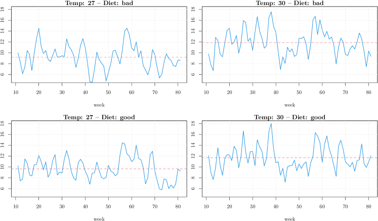
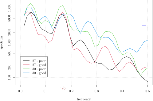
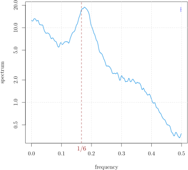
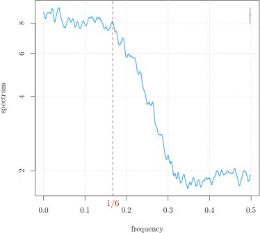
Next, we fit a threshold model to the 4 time series obtained by averaging over the 3 experimental replications. The time plots of series and the results of the tests are presented in Figure 1 and Table 8, respectively. Clearly, warming has a noticeable effect on the mean of the series (dashed red lines). Figure 2 reports the power spectral density of the series. The frequency corresponding to the characteristic asymmetric 6-week generation cycle is evidenced with a red dashed line.

temp. diet statistic p.value
27 poor 10.67 0.055
27 good 15.68 0.006
30 poor 22.13 0.000
30 good 8.02 0.120
Table 8: Results of the application of the sLM tests to the time series of 4 populations of larvae of the pyralid moth P. interpunctella under different experimental conditions: temperature (first column), quality of the diet (second column). The fourth column reports the value of the sLM test statistic, whereas the last column contains the bootstrap p𝑝p-values of our test.
Refer to caption
Figure 1: Time series of 4 populations of P. interpunctella from week 11 to 82 for different experimental conditions. The series have been square-root transformed.
Refer to caption
Figure 2: Power spectrum of the time series of 4 populations of P. interpunctella corresponding to different experimental conditions. The frequency corresponding to the characteristic 6-week cycle is evidenced with a vertical dashed line.

The series are likely to be affected by measurement error so that a threshold ARMA specification is more appropriate than the TAR model (see Chan et al. (2021) for the theoretical justification). Typically, the MA parameters greatly enhance the flexibility of the model, while retaining parsimony Goracci (2020a, b). Hence, we fit the following TARMA model

Xt={ϕ1,0+ϕ1,1Xt1+ϕ1,5Xt5+θ1,1εt1+εt, if Xt2r,ϕ2,0+ϕ2,1Xt1+ϕ2,5Xt5+θ2,3εt3+εt, otherwise.subscript𝑋𝑡casessubscriptitalic-ϕ10subscriptitalic-ϕ11subscript𝑋𝑡1subscriptitalic-ϕ15subscript𝑋𝑡5subscript𝜃11subscript𝜀𝑡1subscript𝜀𝑡 if subscript𝑋𝑡2𝑟subscriptitalic-ϕ20subscriptitalic-ϕ21subscript𝑋𝑡1subscriptitalic-ϕ25subscript𝑋𝑡5subscript𝜃23subscript𝜀𝑡3subscript𝜀𝑡 otherwiseX_{t}=\begin{cases}\phi_{1,0}+\phi_{1,1}X_{t-1}+\phi_{1,5}X_{t-5}+\theta_{1,1}\varepsilon_{t-1}+\varepsilon_{t},&\text{ if }X_{t-2}\leq r,\\ \phi_{2,0}+\phi_{2,1}X_{t-1}+\phi_{2,5}X_{t-5}+\theta_{2,3}\varepsilon_{t-3}+\varepsilon_{t},&\text{ otherwise}.\end{cases} (29)

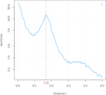
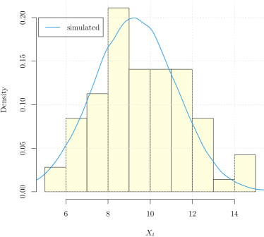
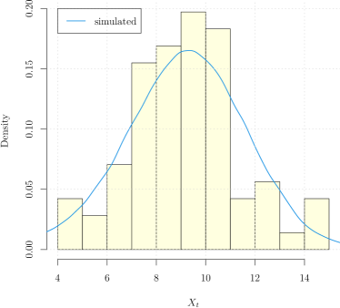
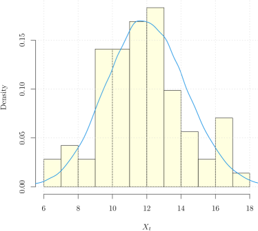
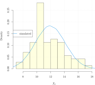
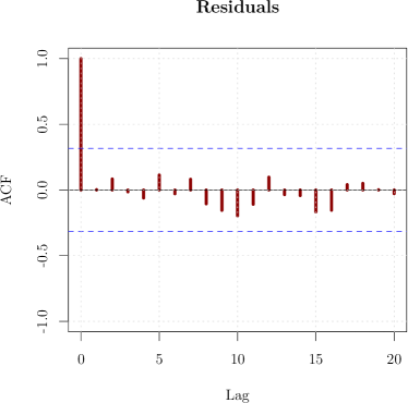
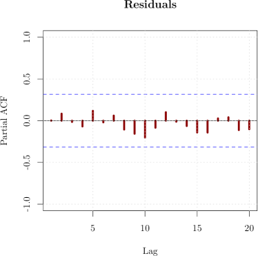
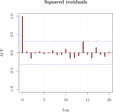
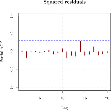
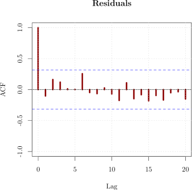
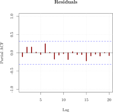
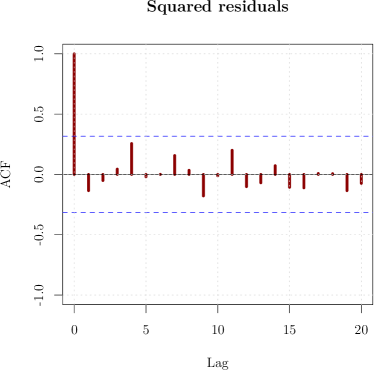
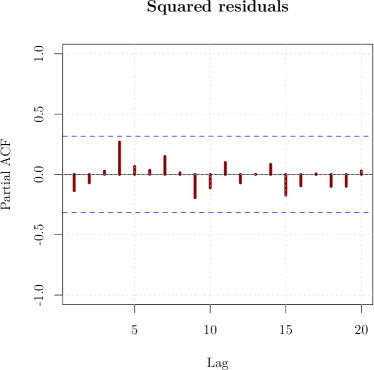
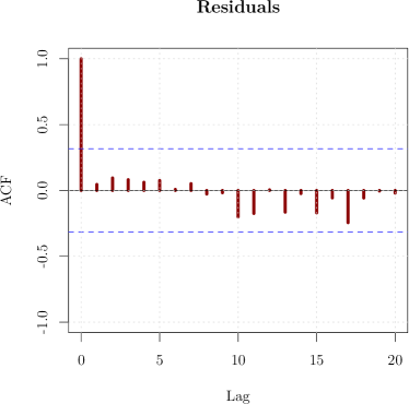
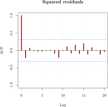
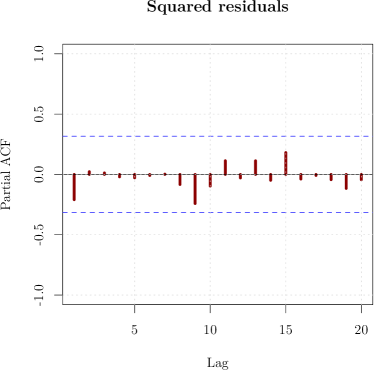
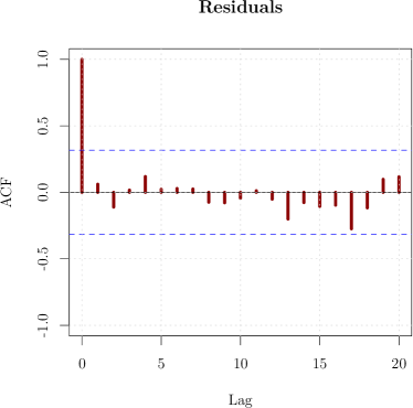
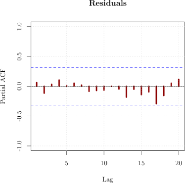
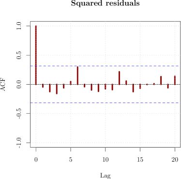
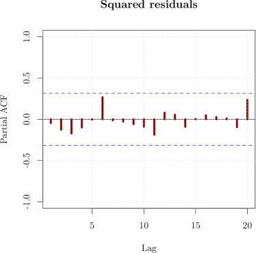
The results are shown in Table 9, where the standard error are reported in parenthesis below the estimates. The last column reports the estimated threshold r^^𝑟\hat{r}. Due to the length of the series, the standard errors are quite large, still, there are both common features and differences across regimes and for different temperatures. Most importantly, the three-lag specification is consistent with the findings of Briggs et al. (2000) and manages to reproduce the characteristic 6-week generation cycle, especially for the series corresponding to a temperature of 27°. This is shown in Figure 3 (left) that shows the power spectral density computed on a series of 100,000 observations simulated from the second fit. The right panel of the figure shows also the histogram of the data with the density of the fitted model, estimated upon the simulated series (blue line). The plots for the other series can be found in the Supplement, Figures 68. The fourth series (30° - good diet) seems to present different periodicities and the model fit is less satisfactory. This could be an indication of the effect of warming producing a qualitative change in the population dynamics. The diagnostic analysis performed both on the residuals and on the squared residuals of the fitted models does not show any unaccounted dependence, see Figures 912 of the Supplementary Material. Finally, the Shapiro-Wilk test applied to the residuals (see Table 2 of the Supplementary Material) does not show departures from normality, except for the last series whose p𝑝p-value 0.046 somehow confirms that the combined action of warming and diet conditions can alter significantly the population dynamics of larvae.

temp diet ϕ^1,0subscript^italic-ϕ10\hat{\phi}_{1,0} ϕ^1,1subscript^italic-ϕ11\hat{\phi}_{1,1} ϕ^1,5subscript^italic-ϕ15\hat{\phi}_{1,5} θ^1,1subscript^𝜃11\hat{\theta}_{1,1} ϕ^2,0subscript^italic-ϕ20\hat{\phi}_{2,0} ϕ^2,1subscript^italic-ϕ21\hat{\phi}_{2,1} ϕ^2,5subscript^italic-ϕ25\hat{\phi}_{2,5} θ^2,3subscript^𝜃23\hat{\theta}_{2,3} r^^𝑟\hat{r}
27 poor 1.15 0.60 0.32 0.61 0.17 0.79 0.15 -0.36 9.18
\rowfont (2.38) (0.21) (0.15) (0.21) (1.37) (0.13) (0.09) (0.18)
27 good 0.73 0.69 0.31 0.24 0.24 0.72 0.19 -0.06 8.89
\rowfont (2.47) (0.30) (0.14) (0.41) (1.53) (0.12) (0.11) (0.17)
30 poor 3.39 0.58 0.22 0.32 1.29 0.66 0.11 0.40 11.93
\rowfont (2.64) (0.19) (0.12) (0.23) (2.29) (0.12) (0.12) (0.20)
30 good 7.00 0.10 0.32 0.40 7.62 0.44 -0.09 -0.18 10.72
\rowfont (5.43) (0.42) (0.19) (0.35) (2.09) (0.13) (0.13) (0.15)
Table 9: Estimated parameters for the threshold ARMA model of Eq. (29) fitted to the time series of populations of larvae under four different experimental conditions. The standard errors are reported in parenthesis below the estimates.
Refer to caption
Refer to caption
Figure 3: (Left) Power spectral density of the simulated time series of 100k observations from the model fit of the second time series (temp: 27°, diet: good). The frequency corresponding to the characteristic 6-week cycle is evidenced with a vertical dashed line.(Right) Histogram of the data (yellow) with the superimposed density of the fitted model, estimated upon the simulated series (blue line).

6 Proofs

Proof of Proposition 3

PART 1. The proof is divided in two parts: first, we show Eq. (23) for a given r𝑟r and then we prove that the result holds also uniformly for r[rL,rU]𝑟subscript𝑟𝐿subscript𝑟𝑈r\in[r_{L},r_{U}].

Pointwise convergence. We assume r𝑟r to be fixed and, for each η>0𝜂0\eta>0, we show that

P(|1nt=1nXtuI(Xtr)E[XtuI(Xtr)]|>2η)n𝑝0.𝑛𝑝superscript𝑃1𝑛superscriptsubscript𝑡1𝑛subscriptsuperscript𝑋absent𝑢𝑡𝐼subscriptsuperscript𝑋𝑡𝑟𝐸delimited-[]subscriptsuperscript𝑋𝑢𝑡𝐼subscript𝑋𝑡𝑟2𝜂0P^{*}\left(\left|\frac{1}{n}\sum_{t=1}^{n}X^{*u}_{t}I(X^{*}_{t}\leq r)-E[X^{u}_{t}I(X_{t}\leq r)]\right|>2\eta\right)\xrightarrow[n\to\infty]{p}0. (30)

Since the indicator function I(yr)𝐼𝑦𝑟I(y\leq r) is not differentiable, standard methods based upon Taylor’s expansion cannot be applied. We exploit the fact that the function is discontinuous only at r𝑟r. By extending the approach used in Chan et al. (2020), we approximate the step function with a sequence of continuous and differentiable functions Gα(y)subscript𝐺𝛼𝑦G_{\alpha}(y), parameterized by α0𝛼0\alpha\geq 0:

Gα(y)={12+1πarctan(ryα)if yr12if y=rsubscript𝐺𝛼𝑦cases121𝜋𝑟𝑦𝛼if 𝑦𝑟12if 𝑦𝑟G_{\alpha}(y)=\begin{cases}\frac{1}{2}+\frac{1}{\pi}\arctan(\frac{r-y}{\alpha})&\mbox{if }y\neq r\\ \frac{1}{2}&\mbox{if }y=r\end{cases} (31)

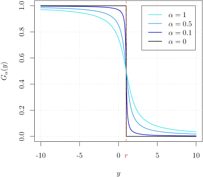
In Figure 4 we show the plot of Gα(y)subscript𝐺𝛼𝑦G_{\alpha}(y) for three values of α𝛼\alpha, together with the limit value α=0𝛼0\alpha=0 for which Gα(y)=I(yr)subscript𝐺𝛼𝑦𝐼𝑦𝑟G_{\alpha}(y)=I(y\leq r) almost surely.

Refer to caption
Figure 4: Gα(y)subscript𝐺𝛼𝑦G_{\alpha}(y) for α=1,0.5,0.1𝛼10.50.1\alpha=1,0.5,0.1, together with the limit value α=0𝛼0\alpha=0 for which Gα(y)=I(yr)subscript𝐺𝛼𝑦𝐼𝑦𝑟G_{\alpha}(y)=I(y\leq r) almost surely.

For each δ>0𝛿0\delta>0, define the interval

[Lα,δ,Uα,δ]:=r±qα,δ,assignsubscript𝐿𝛼𝛿subscript𝑈𝛼𝛿plus-or-minus𝑟subscript𝑞𝛼𝛿[L_{\alpha,\delta},U_{\alpha,\delta}]:=r\pm q_{\alpha,\delta}, (32)

where qα,δ=αtan(π(δ1/2))subscript𝑞𝛼𝛿𝛼𝜋𝛿12q_{\alpha,\delta}=\alpha\tan(\pi(\delta-1/2)). This implies:

|I(yr)Gα(y)|<δ𝐼𝑦𝑟subscript𝐺𝛼𝑦𝛿\displaystyle\left|I(y\leq r)-G_{\alpha}(y)\right|<\delta if y[Lα,δ,Uα,δ];if 𝑦subscript𝐿𝛼𝛿subscript𝑈𝛼𝛿\displaystyle\text{ if }y\notin[L_{\alpha,\delta},U_{\alpha,\delta}]; (33)
|I(yr)Gα(y)|<1𝐼𝑦𝑟subscript𝐺𝛼𝑦1\displaystyle\left|I(y\leq r)-G_{\alpha}(y)\right|<1 if y[Lα,δ,Uα,δ].if 𝑦subscript𝐿𝛼𝛿subscript𝑈𝛼𝛿\displaystyle\text{ if }y\in[L_{\alpha,\delta},U_{\alpha,\delta}]. (34)

Conditions Eq. (32)–(34) assure that, when α𝛼\alpha and δ𝛿\delta approach zero, the interval [Lα,δ,Uα,δ]subscript𝐿𝛼𝛿subscript𝑈𝛼𝛿[L_{\alpha,\delta},U_{\alpha,\delta}] collapses on r𝑟r and the distance between Gα()subscript𝐺𝛼G_{\alpha}(\cdot) and I(r)I(\cdot\leq r), which is bounded by δ𝛿\delta, vanishes. Now, it holds that:

P(|1nt=1nXtuI(Xtr)E[XtuI(Xtr)]|>2η)superscript𝑃1𝑛superscriptsubscript𝑡1𝑛subscriptsuperscript𝑋absent𝑢𝑡𝐼subscriptsuperscript𝑋𝑡𝑟𝐸delimited-[]subscriptsuperscript𝑋𝑢𝑡𝐼subscript𝑋𝑡𝑟2𝜂\displaystyle P^{*}\left(\left|\frac{1}{n}\sum_{t=1}^{n}X^{*u}_{t}I(X^{*}_{t}\leq r)-E[X^{u}_{t}I(X_{t}\leq r)]\right|>2\eta\right)
P(|1nt=1nXtuI(Xtr)1nt=1nXtuGα(Xt)\displaystyle\leq P^{*}\left(\left|\frac{1}{n}\sum_{t=1}^{n}X^{*u}_{t}I(X^{*}_{t}\leq r)-\frac{1}{n}\sum_{t=1}^{n}X^{*u}_{t}G_{\alpha}(X^{*}_{t})\right.\right.
E[XtuI(Xtr)]+E[XtuGα(Xt)]|>η)\displaystyle\phantom{\left(\frac{1}{n}\right)}\left.\left.\phantom{\frac{1}{2}}-E[X^{u}_{t}I(X_{t}\leq r)]+E[X^{u}_{t}G_{\alpha}(X_{t})]\right|>\eta\right) (35)
+P(|1nt=1nXtuGα(Xt)E[XtuGα(Xt)]|>η).superscript𝑃1𝑛superscriptsubscript𝑡1𝑛subscriptsuperscript𝑋absent𝑢𝑡subscript𝐺𝛼subscriptsuperscript𝑋𝑡𝐸delimited-[]subscriptsuperscript𝑋𝑢𝑡subscript𝐺𝛼subscript𝑋𝑡𝜂\displaystyle+P^{*}\left(\left|\frac{1}{n}\sum_{t=1}^{n}X^{*u}_{t}G_{\alpha}(X^{*}_{t})-E[X^{u}_{t}G_{\alpha}(X_{t})]\right|>\eta\right). (36)

Markov’s inequality implies that, in order to prove that Eq. (35) is op(1)subscript𝑜superscript𝑝1o_{p^{*}}(1), it suffices to show that the following two expectations vanish in probability:

E[|E[XtuI(Xtr)]E[XtuGα(Xt)]|],superscript𝐸delimited-[]𝐸delimited-[]subscriptsuperscript𝑋𝑢𝑡𝐼subscript𝑋𝑡𝑟𝐸delimited-[]subscriptsuperscript𝑋𝑢𝑡subscript𝐺𝛼subscript𝑋𝑡\displaystyle E^{*}\left[\left|E[X^{u}_{t}I(X_{t}\leq r)]-E[X^{u}_{t}G_{\alpha}(X_{t})]\right|\right], (37)
E[|1nt=1nXtuI(Xtr)1nt=1nXtuGα(Xt)|].superscript𝐸delimited-[]1𝑛superscriptsubscript𝑡1𝑛subscriptsuperscript𝑋absent𝑢𝑡𝐼subscriptsuperscript𝑋𝑡𝑟1𝑛superscriptsubscript𝑡1𝑛subscriptsuperscript𝑋absent𝑢𝑡subscript𝐺𝛼subscriptsuperscript𝑋𝑡\displaystyle E^{*}\left[\left|\frac{1}{n}\sum_{t=1}^{n}X^{*u}_{t}I(X^{*}_{t}\leq r)-\frac{1}{n}\sum_{t=1}^{n}X^{*u}_{t}G_{\alpha}(X^{*}_{t})\right|\right]. (38)

As for Eq. (37): let fX()subscript𝑓𝑋f_{X}(\cdot) be the stationary probability density function of the AR(p)𝑝(p) process {Xt}subscript𝑋𝑡\{X_{t}\}. Since it is continuous (see e.g. Anděl and Hrach, 2000, theorem 1.3) and E[|Xt|u]<𝐸delimited-[]superscriptsubscript𝑋𝑡𝑢E[|X_{t}|^{u}]<\infty, by using the same argument developed in Ling and Tong (2005), it is possible to show that there exists a positive finite constant, say M𝑀M, such that supx|x|ufX(x)<Msubscriptsupremum𝑥superscript𝑥𝑢subscript𝑓𝑋𝑥𝑀\sup_{x\in\mathds{R}}|x|^{u}f_{X}(x)<M. It holds that:

E[|E[XtuI(Xtr)]E[XtuGα(Xt)]|]=|E[XtuI(Xtr)]E[XtuGα(Xt)]|superscript𝐸delimited-[]𝐸delimited-[]subscriptsuperscript𝑋𝑢𝑡𝐼subscript𝑋𝑡𝑟𝐸delimited-[]subscriptsuperscript𝑋𝑢𝑡subscript𝐺𝛼subscript𝑋𝑡𝐸delimited-[]subscriptsuperscript𝑋𝑢𝑡𝐼subscript𝑋𝑡𝑟𝐸delimited-[]subscriptsuperscript𝑋𝑢𝑡subscript𝐺𝛼subscript𝑋𝑡\displaystyle E^{*}\left[\left|E[X^{u}_{t}I(X_{t}\leq r)]-E[X^{u}_{t}G_{\alpha}(X_{t})]\right|\right]=\left|E[X^{u}_{t}I(X_{t}\leq r)]-E[X^{u}_{t}G_{\alpha}(X_{t})]\right|
E[|Xtu||I(Xtr)Gα(Xt)|]absent𝐸delimited-[]subscriptsuperscript𝑋𝑢𝑡𝐼subscript𝑋𝑡𝑟subscript𝐺𝛼subscript𝑋𝑡\displaystyle\leq E[|X^{u}_{t}|\cdot|I(X_{t}\leq r)-G_{\alpha}(X_{t})|]
=E[|Xtu||I(Xtr)Gα(Xt)|I(Xt[Lα,δ,Uα,δ])]absent𝐸delimited-[]subscriptsuperscript𝑋𝑢𝑡𝐼subscript𝑋𝑡𝑟subscript𝐺𝛼subscript𝑋𝑡𝐼subscript𝑋𝑡subscript𝐿𝛼𝛿subscript𝑈𝛼𝛿\displaystyle=E[|X^{u}_{t}|\cdot|I(X_{t}\leq r)-G_{\alpha}(X_{t})|I(X_{t}\notin[L_{\alpha,\delta},U_{\alpha,\delta}])]
+E[|Xtu||I(Xtr)Gα(Xt)|I(Xt[Lα,δ,Uα,δ])]𝐸delimited-[]subscriptsuperscript𝑋𝑢𝑡𝐼subscript𝑋𝑡𝑟subscript𝐺𝛼subscript𝑋𝑡𝐼subscript𝑋𝑡subscript𝐿𝛼𝛿subscript𝑈𝛼𝛿\displaystyle+E[|X^{u}_{t}|\cdot|I(X_{t}\leq r)-G_{\alpha}(X_{t})|I(X_{t}\in[L_{\alpha,\delta},U_{\alpha,\delta}])]
δE[|Xt|u]+M(Uα,δLα,δ),absent𝛿𝐸delimited-[]superscriptsubscript𝑋𝑡𝑢𝑀subscript𝑈𝛼𝛿subscript𝐿𝛼𝛿\displaystyle\leq\delta E[|X_{t}|^{u}]+M(U_{\alpha,\delta}-L_{\alpha,\delta}),

where the last inequality follows from Eq. (32), Eq. (33) and Eq. (34). Hence, Eq. (37) can be made arbitrarily small in probability by choosing α𝛼\alpha and δ𝛿\delta sufficiently small. A similar argument handles Eq. (38):

E[|1nt=1nXtuI(Xtr)1nt=1nXtuGα(Xt)|]superscript𝐸delimited-[]1𝑛superscriptsubscript𝑡1𝑛subscriptsuperscript𝑋absent𝑢𝑡𝐼subscriptsuperscript𝑋𝑡𝑟1𝑛superscriptsubscript𝑡1𝑛subscriptsuperscript𝑋absent𝑢𝑡subscript𝐺𝛼subscriptsuperscript𝑋𝑡\displaystyle E^{*}\left[\left|\frac{1}{n}\sum_{t=1}^{n}X^{*u}_{t}I(X^{*}_{t}\leq r)-\frac{1}{n}\sum_{t=1}^{n}X^{*u}_{t}G_{\alpha}(X^{*}_{t})\right|\right]
E[1nt=1n|Xtu||I(Xtr)Gα(Xt)|]absentsuperscript𝐸delimited-[]1𝑛superscriptsubscript𝑡1𝑛subscriptsuperscript𝑋absent𝑢𝑡𝐼subscriptsuperscript𝑋𝑡𝑟subscript𝐺𝛼subscriptsuperscript𝑋𝑡\displaystyle\leq E^{*}\left[\frac{1}{n}\sum_{t=1}^{n}|X^{*u}_{t}|\cdot|I(X^{*}_{t}\leq r)-G_{\alpha}(X^{*}_{t})|\right]
=E[1nt=1n|Xtu||I(Xtr)Gα(Xt)|I(Xt[Lα,δ,Uα,δ])]absentsuperscript𝐸delimited-[]1𝑛superscriptsubscript𝑡1𝑛subscriptsuperscript𝑋absent𝑢𝑡𝐼subscriptsuperscript𝑋𝑡𝑟subscript𝐺𝛼subscriptsuperscript𝑋𝑡𝐼subscriptsuperscript𝑋𝑡subscript𝐿𝛼𝛿subscript𝑈𝛼𝛿\displaystyle=E^{*}\left[\frac{1}{n}\sum_{t=1}^{n}|X^{*u}_{t}|\cdot|I(X^{*}_{t}\leq r)-G_{\alpha}(X^{*}_{t})|I(X^{*}_{t}\notin[L_{\alpha,\delta},U_{\alpha,\delta}])\right]
+E[1nt=1n|Xtu||I(Xtr)Gα(Xt)|I(Xt[Lα,δ,Uα,δ])]superscript𝐸delimited-[]1𝑛superscriptsubscript𝑡1𝑛subscriptsuperscript𝑋absent𝑢𝑡𝐼subscriptsuperscript𝑋𝑡𝑟subscript𝐺𝛼subscriptsuperscript𝑋𝑡𝐼subscriptsuperscript𝑋𝑡subscript𝐿𝛼𝛿subscript𝑈𝛼𝛿\displaystyle+E^{*}\left[\frac{1}{n}\sum_{t=1}^{n}|X^{*u}_{t}|\cdot|I(X^{*}_{t}\leq r)-G_{\alpha}(X^{*}_{t})|I(X^{*}_{t}\in[L_{\alpha,\delta},U_{\alpha,\delta}])\right]
δ1nt=1nE[|Xtu|]+1nt=1nP(Xt[Lα,δ,Uα,δ]),absent𝛿1𝑛superscriptsubscript𝑡1𝑛superscript𝐸delimited-[]subscriptsuperscript𝑋absent𝑢𝑡1𝑛superscriptsubscript𝑡1𝑛superscript𝑃subscriptsuperscript𝑋𝑡subscript𝐿𝛼𝛿subscript𝑈𝛼𝛿\displaystyle\leq\delta\frac{1}{n}\sum_{t=1}^{n}E^{*}[|X^{*u}_{t}|]+\mathcal{M}\frac{1}{n}\sum_{t=1}^{n}P^{*}(X^{*}_{t}\in[L_{\alpha,\delta},U_{\alpha,\delta}]),

where =max{|Lα,δ|u,|Uα,δ|u,1}superscriptsubscript𝐿𝛼𝛿𝑢superscriptsubscript𝑈𝛼𝛿𝑢1\mathcal{M}=\max\{|L_{\alpha,\delta}|^{u},|U_{\alpha,\delta}|^{u},1\}. Lemma 10 implies that n1t=1nP(Xt[Lα,δ,Uα,δ])n1superscript𝑛1superscriptsubscript𝑡1𝑛superscript𝑃subscriptsuperscript𝑋𝑡subscript𝐿𝛼𝛿subscript𝑈𝛼𝛿superscript𝑛1n^{-1}\sum_{t=1}^{n}P^{*}(X^{*}_{t}\in[L_{\alpha,\delta},U_{\alpha,\delta}])\leq n^{-1} with probability 1, hence Eq. (38) is op(1)subscript𝑜superscript𝑝1o_{p^{*}}(1). Lastly, in order to show that also Eq. (36) is op(1)subscript𝑜superscript𝑝1o_{p^{*}}(1), we use the following two expansions:

Gα(Xt)=Gα(Xt)+gα(Yt)(XtXt);subscript𝐺𝛼superscriptsubscript𝑋𝑡subscript𝐺𝛼subscript𝑋𝑡subscript𝑔𝛼superscriptsubscript𝑌𝑡superscriptsubscript𝑋𝑡subscript𝑋𝑡\displaystyle G_{\alpha}(X_{t}^{*})=G_{\alpha}(X_{t})+g_{\alpha}(Y_{t}^{*})(X_{t}^{*}-X_{t}); (39)
Gα(Xt)=Gα(qα,δ+2r)+gα(Yt)(Xtqα,δ2r)subscript𝐺𝛼subscript𝑋𝑡subscript𝐺𝛼subscript𝑞𝛼𝛿2𝑟subscript𝑔𝛼subscript𝑌𝑡subscript𝑋𝑡subscript𝑞𝛼𝛿2𝑟\displaystyle G_{\alpha}(X_{t})=G_{\alpha}(q_{\alpha,\delta}+2r)+g_{\alpha}(Y_{t})(X_{t}-q_{\alpha,\delta}-2r) (40)

where qα,δsubscript𝑞𝛼𝛿q_{\alpha,\delta} is defined in Eq. (32), Yt=λ1,tXt+(1λ1,t)Xtsuperscriptsubscript𝑌𝑡subscript𝜆1𝑡subscriptsuperscript𝑋𝑡1subscript𝜆1𝑡subscript𝑋𝑡Y_{t}^{*}=\lambda_{1,t}X^{*}_{t}+(1-\lambda_{1,t})X_{t} and Yt=λ2,tXt+(1λ2,t)(qδ+2r)subscript𝑌𝑡subscript𝜆2𝑡subscript𝑋𝑡1subscript𝜆2𝑡subscript𝑞𝛿2𝑟Y_{t}=\lambda_{2,t}X_{t}+(1-\lambda_{2,t})(q_{\delta}+2r) for some λj,tsubscript𝜆𝑗𝑡\lambda_{j,t} with 0λj,t10subscript𝜆𝑗𝑡10\leq\lambda_{j,t}\leq 1 and j=1,2𝑗12j=1,2; moreover,

gα(y)=Gα(y)y={απ(α2+(ry)2)if yr0if y=r.subscript𝑔𝛼𝑦subscript𝐺𝛼𝑦𝑦cases𝛼𝜋superscript𝛼2superscript𝑟𝑦2if 𝑦𝑟0if 𝑦𝑟g_{\alpha}(y)=\frac{\partial G_{\alpha}(y)}{\partial y}=\begin{cases}-\frac{\alpha}{\pi(\alpha^{2}+(r-y)^{2})}&\mbox{if }y\neq r\\ 0&\mbox{if }y=r.\end{cases}

Note that gα(y)α00 for each y𝛼0absentsubscript𝑔𝛼𝑦0 for each 𝑦g_{\alpha}(y)\xrightarrow[\alpha\rightarrow 0]{}0\text{ for each }y. Since the ergodicity of {Xt}subscript𝑋𝑡\{X_{t}\} implies that

1nt=1nXtuGα(Xt)n𝑝E[XtuGα(Xt)],𝑛𝑝1𝑛superscriptsubscript𝑡1𝑛subscriptsuperscript𝑋𝑢𝑡subscript𝐺𝛼subscript𝑋𝑡𝐸delimited-[]subscriptsuperscript𝑋𝑢𝑡subscript𝐺𝛼subscript𝑋𝑡\frac{1}{n}\sum_{t=1}^{n}X^{u}_{t}G_{\alpha}(X_{t})\xrightarrow[n\to\infty]{p}E[X^{u}_{t}G_{\alpha}(X_{t})],

it suffices to prove that

P(|1nt=1nXtuGα(Xt)1nt=1nXtuGα(Xt)|>η/2)n𝑝0,𝑛𝑝superscript𝑃1𝑛superscriptsubscript𝑡1𝑛subscriptsuperscript𝑋absent𝑢𝑡subscript𝐺𝛼subscriptsuperscript𝑋𝑡1𝑛superscriptsubscript𝑡1𝑛subscriptsuperscript𝑋𝑢𝑡subscript𝐺𝛼subscript𝑋𝑡𝜂20\displaystyle P^{*}\left(\left|\frac{1}{n}\sum_{t=1}^{n}X^{*u}_{t}G_{\alpha}(X^{*}_{t})-\frac{1}{n}\sum_{t=1}^{n}X^{u}_{t}G_{\alpha}(X_{t})\right|>\eta/2\right)\xrightarrow[n\to\infty]{p}0, (41)

which can be achieved by using Markov’s inequality. Indeed, by using Eq. (39), Eq. (40) and since Gα(qδ+2r)=δsubscript𝐺𝛼subscript𝑞𝛿2𝑟𝛿G_{\alpha}(q_{\delta}+2r)=\delta we have

E[|1nt=1nXtuGα(Xt)1nt=1nXtuGα(Xt)|]superscript𝐸delimited-[]1𝑛superscriptsubscript𝑡1𝑛subscriptsuperscript𝑋absent𝑢𝑡subscript𝐺𝛼subscriptsuperscript𝑋𝑡1𝑛superscriptsubscript𝑡1𝑛subscriptsuperscript𝑋𝑢𝑡subscript𝐺𝛼subscript𝑋𝑡\displaystyle E^{*}\left[\left|\frac{1}{n}\sum_{t=1}^{n}X^{*u}_{t}G_{\alpha}(X^{*}_{t})-\frac{1}{n}\sum_{t=1}^{n}X^{u}_{t}G_{\alpha}(X_{t})\right|\right]
E[|1nt=1n(XtuXtu){δ+gα(Yt)(Xtqδ2r)}|]absentsuperscript𝐸delimited-[]1𝑛superscriptsubscript𝑡1𝑛subscriptsuperscript𝑋absent𝑢𝑡subscriptsuperscript𝑋𝑢𝑡𝛿subscript𝑔𝛼subscript𝑌𝑡subscript𝑋𝑡subscript𝑞𝛿2𝑟\displaystyle\leq E^{*}\left[\left|\frac{1}{n}\sum_{t=1}^{n}(X^{*u}_{t}-X^{u}_{t})\left\{\delta+g_{\alpha}(Y_{t})(X_{t}-q_{\delta}-2r)\right\}\right|\right]
+E[|1nt=1nXtugα(Yt)(XtXt)|]superscript𝐸delimited-[]1𝑛superscriptsubscript𝑡1𝑛subscriptsuperscript𝑋absent𝑢𝑡subscript𝑔𝛼superscriptsubscript𝑌𝑡subscriptsuperscript𝑋𝑡subscript𝑋𝑡\displaystyle+E^{*}\left[\left|\frac{1}{n}\sum_{t=1}^{n}X^{*u}_{t}g_{\alpha}(Y_{t}^{*})(X^{*}_{t}-X_{t})\right|\right]

which can be made arbitrarily small in probability by taking α𝛼\alpha and δ𝛿\delta sufficiently small and this completes the proof.

Uniform convergence. By deploying arguments similar to Cavaliere et al. (2017), we show that for each η>0𝜂0\eta>0

P(supr[rL,rU]|Δn(r)|>2η)n𝑝0,𝑛𝑝superscript𝑃subscriptsupremum𝑟subscript𝑟𝐿subscript𝑟𝑈superscriptsubscriptΔ𝑛𝑟2𝜂0P^{*}\left(\sup_{r\in[r_{L},r_{U}]}\left|\Delta_{n}^{*}(r)\right|>2\eta\right)\xrightarrow[n\to\infty]{p}0, (42)

where Δn(r)=n1t=1nXtuI(Xtr)E[XtuI(Xtr)]superscriptsubscriptΔ𝑛𝑟superscript𝑛1superscriptsubscript𝑡1𝑛subscriptsuperscript𝑋absent𝑢𝑡𝐼subscriptsuperscript𝑋𝑡𝑟𝐸delimited-[]subscriptsuperscript𝑋𝑢𝑡𝐼subscript𝑋𝑡𝑟\Delta_{n}^{*}(r)=n^{-1}\sum_{t=1}^{n}X^{*u}_{t}I(X^{*}_{t}\leq r)-E[X^{u}_{t}I(X_{t}\leq r)]. Since [rL,rU]subscript𝑟𝐿subscript𝑟𝑈[r_{L},r_{U}] is a compact subset of \mathds{R}, for any c>0𝑐0c>0, there exists a finite coverage {[ri1,ri];i=1,,m}formulae-sequencesubscript𝑟𝑖1subscript𝑟𝑖𝑖1𝑚\{[r_{i-1},r_{i}];i=1,\dots,m\}, with m𝑚m being a constant, such that rL=r0<r1<<rm1<rm=rUsubscript𝑟𝐿subscript𝑟0subscript𝑟1subscript𝑟𝑚1subscript𝑟𝑚subscript𝑟𝑈r_{L}=r_{0}<r_{1}<\ldots<r_{m-1}<r_{m}=r_{U} ad riri1csubscript𝑟𝑖subscript𝑟𝑖1𝑐r_{i}-r_{i-1}\leq c, for each i=1,,m𝑖1𝑚i=1,\ldots,m. Therefore, it holds that

supr[rL,rU]|Δn(r)|maxi=0,,m|Δn(ri)|+maxi=1,,msupr[ri1,ri]|Δn(r)Δn(ri1)|subscriptsupremum𝑟subscript𝑟𝐿subscript𝑟𝑈superscriptsubscriptΔ𝑛𝑟subscript𝑖0𝑚superscriptsubscriptΔ𝑛subscript𝑟𝑖subscript𝑖1𝑚subscriptsupremum𝑟subscript𝑟𝑖1subscript𝑟𝑖superscriptsubscriptΔ𝑛𝑟superscriptsubscriptΔ𝑛subscript𝑟𝑖1\sup_{r\in[r_{L},r_{U}]}\left|\Delta_{n}^{*}(r)\right|\leq\max_{i=0,\ldots,m}\left|\Delta_{n}^{*}(r_{i})\right|+\max_{i=1,\ldots,m}\sup_{r\in[r_{i-1},r_{i}]}\left|\Delta_{n}^{*}(r)-\Delta_{n}^{*}(r_{i-1})\right|

which implies:

P(supr[rL,rU]|Δn(r)|>2η)superscript𝑃subscriptsupremum𝑟subscript𝑟𝐿subscript𝑟𝑈superscriptsubscriptΔ𝑛𝑟2𝜂\displaystyle P^{*}\left(\sup_{r\in[r_{L},r_{U}]}\left|\Delta_{n}^{*}(r)\right|>2\eta\right)
P(maxi=0,,m|Δn(ri)|>η)+P(maxi=1,,msupr[ri1,ri]|Δn(r)Δn(ri1)|>η)absentsuperscript𝑃subscript𝑖0𝑚superscriptsubscriptΔ𝑛subscript𝑟𝑖𝜂superscript𝑃subscript𝑖1𝑚subscriptsupremum𝑟subscript𝑟𝑖1subscript𝑟𝑖superscriptsubscriptΔ𝑛𝑟superscriptsubscriptΔ𝑛subscript𝑟𝑖1𝜂\displaystyle\leq P^{*}\left(\max_{i=0,\ldots,m}\left|\Delta_{n}^{*}(r_{i})\right|>\eta\right)+P^{*}\left(\max_{i=1,\ldots,m}\sup_{r\in[r_{i-1},r_{i}]}\left|\Delta_{n}^{*}(r)-\Delta_{n}^{*}(r_{i-1})\right|>\eta\right) (43)

By combining Bonferroni’s inequality, the pointwise convergence and the finiteness of m𝑚m, we have that

P(maxi=1,,m|Δn(ri)|>η)i=1mP(|Δn(ri)|>η)n𝑝0.superscript𝑃subscript𝑖1𝑚superscriptsubscriptΔ𝑛subscript𝑟𝑖𝜂superscriptsubscript𝑖1𝑚superscript𝑃superscriptsubscriptΔ𝑛subscript𝑟𝑖𝜂𝑛𝑝0P^{*}\left(\max_{i=1,\ldots,m}\left|\Delta_{n}^{*}(r_{i})\right|>\eta\right)\leq\sum_{i=1}^{m}P^{*}\left(\left|\Delta_{n}^{*}(r_{i})\right|>\eta\right)\xrightarrow[n\to\infty]{p}0.

It remains to show that the second term of the RHS of Eq. (43) converges to zero in probability (in probability), which is the case because:

E[supr[ri1,ri]|Δn(r)Δn(ri1)|]superscript𝐸delimited-[]subscriptsupremum𝑟subscript𝑟𝑖1subscript𝑟𝑖superscriptsubscriptΔ𝑛𝑟superscriptsubscriptΔ𝑛subscript𝑟𝑖1\displaystyle E^{*}\left[\sup_{r\in[r_{i-1},r_{i}]}\left|\Delta_{n}^{*}(r)-\Delta_{n}^{*}(r_{i-1})\right|\right]
E[supr[ri1,ri]1nt=1n|Xtu|I(ri1<Xtr)\displaystyle\leq E^{*}\left[\sup_{r\in[r_{i-1},r_{i}]}\frac{1}{n}\sum_{t=1}^{n}|X_{t}^{*u}|I(r_{i-1}<X_{t}^{*}\leq r)\right.
+supr[ri1,ri]E[|Xt|uI(ri1<Xtr)]]\displaystyle\phantom{E^{*}\left[\right.}\phantom{\frac{1}{2}}+\left.\sup_{r\in[r_{i-1},r_{i}]}E[|X_{t}|^{u}I(r_{i-1}<X_{t}\leq r)]\right]
E[1nt=1n|Xtu|I(ri1c<Xtri1+c)+E[|Xt|uI(ri1<Xtri)]]absentsuperscript𝐸delimited-[]1𝑛superscriptsubscript𝑡1𝑛superscriptsubscript𝑋𝑡absent𝑢𝐼subscript𝑟𝑖1𝑐superscriptsubscript𝑋𝑡subscript𝑟𝑖1𝑐𝐸delimited-[]superscriptsubscript𝑋𝑡𝑢𝐼subscript𝑟𝑖1subscript𝑋𝑡subscript𝑟𝑖\displaystyle\leq E^{*}\left[\frac{1}{n}\sum_{t=1}^{n}|X_{t}^{*u}|I(r_{i-1}-c<X_{t}^{*}\leq r_{i-1}+c)+E[|X_{t}|^{u}I(r_{i-1}<X_{t}\leq r_{i})]\right]
1nt=1nP(ri1c<Xtri1+c)+2P(ri1<Xtr),absentsubscript1𝑛superscriptsubscript𝑡1𝑛superscript𝑃subscript𝑟𝑖1𝑐superscriptsubscript𝑋𝑡subscript𝑟𝑖1𝑐subscript2𝑃subscript𝑟𝑖1subscript𝑋𝑡𝑟\displaystyle\leq\frac{\mathcal{M}_{1}}{n}\sum_{t=1}^{n}P^{*}(r_{i-1}-c<X_{t}^{*}\leq r_{i-1}+c)+\mathcal{M}_{2}P(r_{i-1}<X_{t}\leq r),

with 1=max{|ri1c|u,|ri1+c|u,1}subscript1superscriptsubscript𝑟𝑖1𝑐𝑢superscriptsubscript𝑟𝑖1𝑐𝑢1\mathcal{M}_{1}=\max\{|r_{i-1}-c|^{u},|r_{i-1}+c|^{u},1\} and 2=max{|ri1|u,|ri|u,1}subscript2superscriptsubscript𝑟𝑖1𝑢superscriptsubscript𝑟𝑖𝑢1\mathcal{M}_{2}=\max\{|r_{i-1}|^{u},|r_{i}|^{u},1\}. By combining Lemma 10 and Markov’s inequality, the proof is completed since c𝑐c can be chosen arbitrarily small.

PART 2. The proof follows via the same arguments used in 1. and, hence, it is omitted.

Proof of Proposition 5

By routine algebra it holds that In,22(r)=In,12(r)=In,21(r)subscriptsuperscript𝐼𝑛22𝑟subscriptsuperscript𝐼𝑛12𝑟subscriptsuperscript𝐼absent𝑛21𝑟I^{*}_{n,22}(r)=I^{*}_{n,12}(r)=I^{*\;\intercal}_{n,21}(r) are (p+1)×(p+1)𝑝1𝑝1(p+1)\times(p+1) symmetric matrices whose (i+1,j+1)𝑖1𝑗1(i+1,j+1)th element is

t=1nI(Xtdr),superscriptsubscript𝑡1𝑛𝐼subscriptsuperscript𝑋𝑡𝑑𝑟\displaystyle\sum_{t=1}^{n}I(X^{*}_{t-d}\leq r), if i=0,j=0formulae-sequenceif 𝑖0𝑗0\displaystyle\mbox{if }i=0,j=0
t=1nXtjI(Xtdr),superscriptsubscript𝑡1𝑛subscriptsuperscript𝑋𝑡𝑗𝐼subscriptsuperscript𝑋𝑡𝑑𝑟\displaystyle\sum_{t=1}^{n}X^{*}_{t-j}I(X^{*}_{t-d}\leq r), if i=0,j0formulae-sequenceif 𝑖0𝑗0\displaystyle\mbox{if }i=0,j\neq 0
t=1nXtiXtjI(Xtdr),superscriptsubscript𝑡1𝑛subscriptsuperscript𝑋𝑡𝑖subscriptsuperscript𝑋𝑡𝑗𝐼subscriptsuperscript𝑋𝑡𝑑𝑟\displaystyle\sum_{t=1}^{n}X^{*}_{t-i}X^{*}_{t-j}I(X^{*}_{t-d}\leq r), if i0,j0formulae-sequenceif 𝑖0𝑗0\displaystyle\mbox{if }i\neq 0,j\neq 0

and In,11=In,22()subscriptsuperscript𝐼𝑛11subscriptsuperscript𝐼𝑛22I^{*}_{n,11}=I^{*}_{n,22}(\infty). The results readily follows by combining Proposition 3 with u=0,1,2𝑢012u=0,1,2 for point 1 and standard results of bootstrap asymptotic analysis.

Proof of Proposition 6

The proof is based upon verifying the following two equalities:

n(ϕ~ϕ~)𝑛~bold-italic-ϕsuperscript~bold-italic-ϕ\displaystyle\sqrt{n}(\tilde{\boldsymbol{\phi}}-\tilde{\boldsymbol{\phi}}^{*}) =(In,11n)11nnϕabsentsuperscriptsubscriptsuperscript𝐼𝑛11𝑛11𝑛superscriptsubscript𝑛bold-italic-ϕ\displaystyle=-\left(\frac{I^{*}_{n,11}}{n}\right)^{-1}\frac{1}{\sqrt{n}}\frac{\partial\ell_{n}^{*}}{\partial\boldsymbol{\phi}} (44)
1n~n𝚿(r)1𝑛superscriptsubscript~𝑛𝚿𝑟\displaystyle\frac{1}{\sqrt{n}}\frac{\partial\tilde{\ell}_{n}^{*}}{\partial\boldsymbol{\Psi}}(r) =1nn𝚿(r)+In,21(r)nn(ϕ~ϕ~),absent1𝑛superscriptsubscript𝑛𝚿𝑟subscriptsuperscript𝐼𝑛21𝑟𝑛𝑛~bold-italic-ϕsuperscript~bold-italic-ϕ\displaystyle=\frac{1}{\sqrt{n}}\frac{\partial\ell_{n}^{*}}{\partial\boldsymbol{\Psi}}(r)+\frac{I^{*}_{n,21}(r)}{n}\sqrt{n}(\tilde{\boldsymbol{\phi}}-\tilde{\boldsymbol{\phi}}^{*}), (45)

where nϕsuperscriptsubscript𝑛bold-italic-ϕ\frac{\partial\ell_{n}^{*}}{\partial\boldsymbol{\phi}}, n𝚿(r)superscriptsubscript𝑛𝚿𝑟\frac{\partial\ell_{n}^{*}}{\partial\boldsymbol{\Psi}}(r) and ~n𝚿(r)superscriptsubscript~𝑛𝚿𝑟\frac{\partial\tilde{\ell}_{n}^{*}}{\partial\boldsymbol{\Psi}}(r) are defined in Eq. (19) whereas In,11subscriptsuperscript𝐼𝑛11I^{*}_{n,11} and In,21(r)subscriptsuperscript𝐼𝑛21𝑟I^{*}_{n,21}(r) in Eq. (17). As previously state we use ϕbold-italic-ϕ\boldsymbol{\phi} as to refer to a generic parameter and let nϕ(ϕ)superscriptsubscript𝑛bold-italic-ϕbold-italic-ϕ\frac{\partial\ell_{n}^{*}}{\partial\boldsymbol{\phi}}(\boldsymbol{\phi}) be the partial derivative of the bootstrap log-likelihood computed under the null hypothesis, i.e.:

nϕ(ϕ)=n(𝜼,r)𝜼|𝚿=𝟎,σ2=σ~2.superscriptsubscript𝑛bold-italic-ϕbold-italic-ϕevaluated-atsuperscriptsubscript𝑛𝜼𝑟𝜼formulae-sequence𝚿0superscript𝜎2superscript~𝜎2\left.\frac{\partial\ell_{n}^{*}}{\partial\boldsymbol{\phi}}(\boldsymbol{\phi})=\frac{\partial\ell_{n}^{*}(\boldsymbol{\eta},r)}{\partial\boldsymbol{\eta}}\right|_{\boldsymbol{\Psi}=\boldsymbol{0},\sigma^{2}=\tilde{\sigma}^{2}}.

Next, we derive two first order Taylor expansions of the function nϕ(ϕ)superscriptsubscript𝑛bold-italic-ϕbold-italic-ϕ\frac{\partial\ell_{n}^{*}}{\partial\boldsymbol{\phi}}(\boldsymbol{\phi}): one at the true bootstrap value ϕ~~bold-italic-ϕ\tilde{\boldsymbol{\phi}} ad the other at the bootstrap MLE ϕ~superscript~bold-italic-ϕ\tilde{\boldsymbol{\phi}}^{*}. Note that, since the νsuperscript𝜈\nu^{\prime} partial derivatives of n(𝜼,r)superscriptsubscript𝑛𝜼𝑟\ell_{n}^{*}(\boldsymbol{\eta},r) are zero for ν>2𝜈2\nu>2, the Taylor expansion of nϕ(ϕ)superscriptsubscript𝑛bold-italic-ϕbold-italic-ϕ\frac{\partial\ell_{n}^{*}}{\partial\boldsymbol{\phi}}(\boldsymbol{\phi}) coincides with its first-order Taylor polynomial; moreover, the Jacobian matrix of ϕ(ϕ)superscriptbold-italic-ϕbold-italic-ϕ\frac{\partial\ell^{*}}{\partial\boldsymbol{\phi}}(\boldsymbol{\phi}) is In,11subscriptsuperscript𝐼𝑛11-I^{*}_{n,11}, defined in Eq. (17), which does not depend on ϕbold-italic-ϕ\boldsymbol{\phi}. Hence it results that:

nϕ(ϕ)superscriptsubscript𝑛bold-italic-ϕbold-italic-ϕ\displaystyle\frac{\partial\ell_{n}^{*}}{\partial\boldsymbol{\phi}}(\boldsymbol{\phi}) =nϕIn,11(ϕϕ~),absentsuperscriptsubscript𝑛bold-italic-ϕsubscript𝐼𝑛11bold-italic-ϕ~bold-italic-ϕ\displaystyle=\frac{\partial{\ell_{n}}^{*}}{\partial\boldsymbol{\phi}}-I_{n,11}(\boldsymbol{\phi}-\tilde{\boldsymbol{\phi}}), (46)
nϕ(ϕ)superscriptsubscript𝑛bold-italic-ϕbold-italic-ϕ\displaystyle\frac{\partial\ell_{n}^{*}}{\partial\boldsymbol{\phi}}(\boldsymbol{\phi}) =~nϕIn,11(ϕϕ~)absentsuperscriptsubscript~𝑛bold-italic-ϕsubscript𝐼𝑛11bold-italic-ϕsuperscript~bold-italic-ϕ\displaystyle=\frac{\partial\tilde{\ell}_{n}^{*}}{\partial\boldsymbol{\phi}}-I_{n,11}(\boldsymbol{\phi}-\tilde{\boldsymbol{\phi}}^{*}) (47)

with ~nϕsuperscriptsubscript~𝑛bold-italic-ϕ\frac{\partial\tilde{\ell}_{n}^{*}}{\partial\boldsymbol{\phi}} and nϕsuperscriptsubscript𝑛bold-italic-ϕ\frac{\partial{\ell}_{n}^{*}}{\partial\boldsymbol{\phi}} being defined in Eq. (18). By subtracting Eq. (47) from Eq. (46) and dividing by n𝑛\sqrt{n}, we get

1n~nϕ=1nnϕ+In,11nn(ϕ~ϕ~).1𝑛superscriptsubscript~𝑛bold-italic-ϕ1𝑛superscriptsubscript𝑛bold-italic-ϕsuperscriptsubscript𝐼𝑛11𝑛𝑛~bold-italic-ϕsuperscript~bold-italic-ϕ\frac{1}{\sqrt{n}}\frac{\partial\tilde{\ell}_{n}^{*}}{\partial\boldsymbol{\phi}}=\frac{1}{\sqrt{n}}\frac{\partial{\ell}_{n}^{*}}{\partial\boldsymbol{\phi}}+\frac{I_{n,11}^{*}}{n}\sqrt{n}(\tilde{\boldsymbol{\phi}}-\tilde{\boldsymbol{\phi}}^{*}). (48)

Since ϕ~superscript~bold-italic-ϕ\tilde{\boldsymbol{\phi}}^{*} is the bootstrap MLE obtained under the null hypothesis, ~nϕ=0superscriptsubscript~𝑛bold-italic-ϕ0\frac{\partial\tilde{\ell}_{n}^{*}}{\partial\boldsymbol{\phi}}=0 thence Eq. (48) implies

In,11nn(ϕ~ϕ~)=1nnϕ.superscriptsubscript𝐼𝑛11𝑛𝑛superscript~bold-italic-ϕ~bold-italic-ϕ1𝑛superscriptsubscript𝑛bold-italic-ϕ\displaystyle\frac{I_{n,11}^{*}}{n}\sqrt{n}(\tilde{\boldsymbol{\phi}}^{*}-\tilde{\boldsymbol{\phi}})=-\frac{1}{\sqrt{n}}\frac{\partial\ell_{n}^{*}}{\partial\boldsymbol{\phi}}.

and hence Eq. (44) follows. We prove Eq. (45) componentwise. We detail below the argument only for the first component since it can be easily adapted to the other ones. Therefore, we show that:

1n~nΨ0(r)1𝑛superscriptsubscript~𝑛subscriptΨ0𝑟\displaystyle\frac{1}{\sqrt{n}}\frac{\partial\tilde{\ell}_{n}^{*}}{\partial{\Psi_{0}}}(r) =1nnΨ0(r)+n(ϕ~0ϕ~0)1nt=1nI(Xtdr)absent1𝑛superscriptsubscript𝑛subscriptΨ0𝑟𝑛subscript~italic-ϕ0superscriptsubscript~italic-ϕ01𝑛superscriptsubscript𝑡1𝑛𝐼subscriptsuperscript𝑋𝑡𝑑𝑟\displaystyle=\frac{1}{\sqrt{n}}\frac{\partial\ell_{n}^{*}}{\partial{\Psi_{0}}}(r)+\sqrt{n}({\tilde{\phi}_{0}}-{\tilde{\phi}_{0}^{*}})\frac{1}{n}\sum_{t=1}^{n}I(X^{*}_{t-d}\leq r)
+i=1pn(ϕ~iϕ~i)1nt=1nXtiI(Xtdr).superscriptsubscript𝑖1𝑝𝑛subscript~italic-ϕ𝑖superscriptsubscript~italic-ϕ𝑖1𝑛superscriptsubscript𝑡1𝑛subscriptsuperscript𝑋𝑡𝑖𝐼subscriptsuperscript𝑋𝑡𝑑𝑟\displaystyle+\sum_{i=1}^{p}\sqrt{n}({\tilde{\phi}_{i}}-{\tilde{\phi}_{i}^{*}})\frac{1}{n}\sum_{t=1}^{n}X^{*}_{t-i}I(X^{*}_{t-d}\leq r). (49)

Let ε~tsuperscriptsubscript~𝜀𝑡\tilde{\varepsilon}_{t}^{*} be the residuals obtained from the ML fit upon the bootstrap sample {Xt,t=1,n}formulae-sequencesubscriptsuperscript𝑋𝑡𝑡1𝑛\{X^{*}_{t},t=1\dots,n\}, i.e.:

ε~tsubscriptsuperscript~𝜀𝑡\displaystyle\tilde{\varepsilon}^{*}_{t} =Xtϕ~0i=1pϕ~iXti=(ϕ~0ϕ~0)+i=1p(ϕ~iϕ~i)Xti+εt.absentsubscriptsuperscript𝑋𝑡subscriptsuperscript~italic-ϕ0superscriptsubscript𝑖1𝑝subscriptsuperscript~italic-ϕ𝑖subscriptsuperscript𝑋𝑡𝑖subscript~italic-ϕ0subscriptsuperscript~italic-ϕ0superscriptsubscript𝑖1𝑝subscript~italic-ϕ𝑖subscriptsuperscript~italic-ϕ𝑖subscript𝑋𝑡𝑖subscriptsuperscript𝜀𝑡\displaystyle=X^{*}_{t}-\tilde{\phi}^{*}_{0}-\sum_{i=1}^{p}\tilde{\phi}^{*}_{i}X^{*}_{t-i}=(\tilde{\phi}_{0}-\tilde{\phi}^{*}_{0})+\sum_{i=1}^{p}(\tilde{\phi}_{i}-\tilde{\phi}^{*}_{i})X_{t-i}+\varepsilon^{*}_{t}.

Clearly:

εtε~t=(ϕ~0ϕ~0)+i=1p(ϕ~iϕ~i)Xti.superscriptsubscript𝜀𝑡superscriptsubscript~𝜀𝑡superscriptsubscript~italic-ϕ0subscript~italic-ϕ0superscriptsubscript𝑖1𝑝superscriptsubscript~italic-ϕ𝑖subscript~italic-ϕ𝑖superscriptsubscript𝑋𝑡𝑖\varepsilon_{t}^{*}-\tilde{\varepsilon}_{t}^{*}=({\tilde{\phi}_{0}^{*}}-{\tilde{\phi}_{0}})+\sum_{i=1}^{p}({\tilde{\phi}_{i}^{*}}-{\tilde{\phi}_{i}})X_{t-i}^{*}. (50)

Note that εt(𝜼,r)subscriptsuperscript𝜀𝑡𝜼𝑟\varepsilon^{*}_{t}(\boldsymbol{\eta},r), defined in Eq. (15), does not depend on σ2superscript𝜎2\sigma^{2} and ε~tsubscriptsuperscript~𝜀𝑡\tilde{\varepsilon}^{*}_{t} and εtsubscriptsuperscript𝜀𝑡{\varepsilon}^{*}_{t} correspond to the function εt(𝜼,r)subscriptsuperscript𝜀𝑡𝜼𝑟\varepsilon^{*}_{t}(\boldsymbol{\eta},r) evaluated at ϕ=ϕ~bold-italic-ϕsuperscript~bold-italic-ϕ\boldsymbol{\phi}=\tilde{\boldsymbol{\phi}}^{*}, 𝚿=𝟎𝚿0\boldsymbol{\Psi}=\boldsymbol{0} and ϕ=ϕ~bold-italic-ϕ~bold-italic-ϕ\boldsymbol{\phi}=\tilde{\boldsymbol{\phi}}, 𝚿=𝟎𝚿0\boldsymbol{\Psi}=\boldsymbol{0}, respectively. Consider the partial derivatives of the function εt(𝜼,r)subscriptsuperscript𝜀𝑡𝜼𝑟\varepsilon^{*}_{t}(\boldsymbol{\eta},r) and denote:

DΨ0t(r)=εt(𝜼,r)Ψ0|ϕ=ϕ~,𝚿=𝟎,D~Ψ0t(r)=εt(𝜼,r)Ψ0|ϕ=ϕ~,𝚿=𝟎.formulae-sequencesuperscriptsubscript𝐷subscriptΨ0𝑡𝑟evaluated-atsubscriptsuperscript𝜀𝑡𝜼𝑟subscriptΨ0formulae-sequencebold-italic-ϕ~bold-italic-ϕ𝚿0superscriptsubscript~𝐷subscriptΨ0𝑡𝑟evaluated-atsubscriptsuperscript𝜀𝑡𝜼𝑟subscriptΨ0formulae-sequencebold-italic-ϕsuperscript~bold-italic-ϕ𝚿0\left.D_{\Psi_{0}t}^{*}(r)=\frac{\partial\varepsilon^{*}_{t}(\boldsymbol{\eta},r)}{\partial\Psi_{0}}\right|_{\boldsymbol{\phi}=\tilde{\boldsymbol{\phi}},\boldsymbol{\Psi}=\boldsymbol{0}},\quad\left.\tilde{D}_{\Psi_{0}t}^{*}(r)=\frac{\partial\varepsilon^{*}_{t}(\boldsymbol{\eta},r)}{\partial\Psi_{0}}\right|_{\boldsymbol{\phi}=\tilde{\boldsymbol{\phi}}^{*},\boldsymbol{\Psi}=\boldsymbol{0}}.

Note that:

DΨ0t(r)=D~Ψ0t(r)=I(Xtdr)superscriptsubscript𝐷subscriptΨ0𝑡𝑟superscriptsubscript~𝐷subscriptΨ0𝑡𝑟𝐼subscriptsuperscript𝑋𝑡𝑑𝑟D_{\Psi_{0}t}^{*}(r)=\tilde{D}_{\Psi_{0}t}^{*}(r)=-I(X^{*}_{t-d}\leq r)

therefore, we get:

1n~nΨ0(r)1𝑛superscriptsubscript~𝑛subscriptΨ0𝑟\displaystyle\frac{1}{\sqrt{n}}\frac{\partial\tilde{\ell}_{n}^{*}}{\partial{\Psi_{0}}}(r) =1nt=1nε~tD~Ψ0t(r)=1nt=1nε~tDΨ0t(r)absent1𝑛superscriptsubscript𝑡1𝑛superscriptsubscript~𝜀𝑡superscriptsubscript~𝐷subscriptΨ0𝑡𝑟1𝑛superscriptsubscript𝑡1𝑛superscriptsubscript~𝜀𝑡superscriptsubscript𝐷subscriptΨ0𝑡𝑟\displaystyle=-\frac{1}{\sqrt{n}}\sum_{t=1}^{n}\tilde{\varepsilon}_{t}^{*}\tilde{D}_{\Psi_{0}t}^{*}(r)=-\frac{1}{\sqrt{n}}\sum_{t=1}^{n}\tilde{\varepsilon}_{t}^{*}{D}_{\Psi_{0}t}^{*}(r)
=1nt=1nε~tDΨ0t(r)1nt=1nεtDΨ0t(r)+1nt=1nεtDΨ0t(r)absent1𝑛superscriptsubscript𝑡1𝑛superscriptsubscript~𝜀𝑡superscriptsubscript𝐷subscriptΨ0𝑡𝑟1𝑛superscriptsubscript𝑡1𝑛superscriptsubscript𝜀𝑡superscriptsubscript𝐷subscriptΨ0𝑡𝑟1𝑛superscriptsubscript𝑡1𝑛superscriptsubscript𝜀𝑡superscriptsubscript𝐷subscriptΨ0𝑡𝑟\displaystyle=-\frac{1}{\sqrt{n}}\sum_{t=1}^{n}\tilde{\varepsilon}_{t}^{*}{D}_{\Psi_{0}t}^{*}(r)-\frac{1}{\sqrt{n}}\sum_{t=1}^{n}{\varepsilon}_{t}^{*}{D}_{\Psi_{0}t}^{*}(r)+\frac{1}{\sqrt{n}}\sum_{t=1}^{n}{\varepsilon}_{t}^{*}{D}_{\Psi_{0}t}^{*}(r)
=1nnΨ0(r)+1nt=1n(εtε~t)DΨ0t(r).absent1𝑛superscriptsubscript𝑛subscriptΨ0𝑟1𝑛superscriptsubscript𝑡1𝑛superscriptsubscript𝜀𝑡superscriptsubscript~𝜀𝑡superscriptsubscript𝐷subscriptΨ0𝑡𝑟\displaystyle=\frac{1}{\sqrt{n}}\frac{\partial\ell_{n}^{*}}{\partial{\Psi_{0}}}(r)+\frac{1}{\sqrt{n}}\sum_{t=1}^{n}({\varepsilon}_{t}^{*}-\tilde{\varepsilon}_{t}^{*}){D}_{\Psi_{0}t}^{*}(r).

The expression of (εtε~t)superscriptsubscript𝜀𝑡superscriptsubscript~𝜀𝑡({\varepsilon}_{t}^{*}-\tilde{\varepsilon}_{t}^{*}) in Eq. (50) implies that

1n~nΨ0(r)1𝑛superscriptsubscript~𝑛subscriptΨ0𝑟\displaystyle\frac{1}{\sqrt{n}}\frac{\partial\tilde{\ell}_{n}^{*}}{\partial{\Psi_{0}}}(r) =1nnΨ0(r)+1nt=1n{(ϕ~0ϕ~0)+i=1p(ϕ~iϕ~i)Xti}DΨ0t(r)absent1𝑛superscriptsubscript𝑛subscriptΨ0𝑟1𝑛superscriptsubscript𝑡1𝑛superscriptsubscript~italic-ϕ0subscript~italic-ϕ0superscriptsubscript𝑖1𝑝superscriptsubscript~italic-ϕ𝑖subscript~italic-ϕ𝑖superscriptsubscript𝑋𝑡𝑖superscriptsubscript𝐷subscriptΨ0𝑡𝑟\displaystyle=\frac{1}{\sqrt{n}}\frac{\partial\ell_{n}^{*}}{\partial{\Psi_{0}}}(r)+\frac{1}{\sqrt{n}}\sum_{t=1}^{n}\left\{({\tilde{\phi}_{0}^{*}}-{\tilde{\phi}_{0}})+\sum_{i=1}^{p}({\tilde{\phi}_{i}^{*}}-{\tilde{\phi}_{i}})X_{t-i}^{*}\right\}{D}_{\Psi_{0}t}^{*}(r)
=1nnΨ0(r)absent1𝑛superscriptsubscript𝑛subscriptΨ0𝑟\displaystyle=\frac{1}{\sqrt{n}}\frac{\partial\ell_{n}^{*}}{\partial{\Psi_{0}}}(r)
+1nt=1n{(ϕ~0ϕ~0)+i=1p(ϕ~iϕ~i)Xti}{I(Xtdr)}1𝑛superscriptsubscript𝑡1𝑛superscriptsubscript~italic-ϕ0subscript~italic-ϕ0superscriptsubscript𝑖1𝑝superscriptsubscript~italic-ϕ𝑖subscript~italic-ϕ𝑖superscriptsubscript𝑋𝑡𝑖𝐼subscriptsuperscript𝑋𝑡𝑑𝑟\displaystyle+\frac{1}{\sqrt{n}}\sum_{t=1}^{n}\left\{({\tilde{\phi}_{0}^{*}}-{\tilde{\phi}_{0}})+\sum_{i=1}^{p}({\tilde{\phi}_{i}^{*}}-{\tilde{\phi}_{i}})X_{t-i}^{*}\right\}\left\{-I(X^{*}_{t-d}\leq r)\right\}
=1nnΨ0(r)+n(ϕ~0ϕ~0)1nt=1nI(Xtdr)absent1𝑛superscriptsubscript𝑛subscriptΨ0𝑟𝑛subscript~italic-ϕ0superscriptsubscript~italic-ϕ01𝑛superscriptsubscript𝑡1𝑛𝐼subscriptsuperscript𝑋𝑡𝑑𝑟\displaystyle=\frac{1}{\sqrt{n}}\frac{\partial\ell_{n}^{*}}{\partial{\Psi_{0}}}(r)+\sqrt{n}({\tilde{\phi}_{0}}-{\tilde{\phi}_{0}^{*}})\frac{1}{n}\sum_{t=1}^{n}I(X^{*}_{t-d}\leq r)
+i=1pn(ϕ~iϕ~i)1nt=1nXtiI(Xtdr)superscriptsubscript𝑖1𝑝𝑛subscript~italic-ϕ𝑖superscriptsubscript~italic-ϕ𝑖1𝑛superscriptsubscript𝑡1𝑛subscriptsuperscript𝑋𝑡𝑖𝐼subscriptsuperscript𝑋𝑡𝑑𝑟\displaystyle+\sum_{i=1}^{p}\sqrt{n}({\tilde{\phi}_{i}}-{\tilde{\phi}_{i}^{*}})\frac{1}{n}\sum_{t=1}^{n}X^{*}_{t-i}I(X^{*}_{t-d}\leq r)

and this completes the proof.

Proof of Proposition 8

Since n𝜼(r)=t=1nεtDt1(r)superscriptsubscript𝑛𝜼𝑟superscriptsubscript𝑡1𝑛subscriptsuperscript𝜀𝑡subscriptsuperscript𝐷𝑡1𝑟\frac{\partial\ell_{n}^{*}}{\partial\boldsymbol{\eta}}(r)=-\sum_{t=1}^{n}\varepsilon^{*}_{t}D^{*}_{t-1}(r), with Dt(r)subscriptsuperscript𝐷𝑡𝑟D^{*}_{t}(r) being defined in Eq. (3), forms a sequence of martingale difference arrays with respect to the filtration t1:=σ{Xt1,Xt2,}assignsuperscriptsubscript𝑡1𝜎subscriptsuperscript𝑋𝑡1subscriptsuperscript𝑋𝑡2\mathcal{F}_{t-1}^{*}:=\sigma\{X^{*}_{t-1},X^{*}_{t-2},\dots\}, the result holds upon proving, uniformly on r𝑟r, the following two conditions:

1nt=1nE[εt2(Dt1(r))(Dt1(r))|t1]nppσ2I(r);subscript𝑛superscript𝑝𝑝1𝑛superscriptsubscript𝑡1𝑛superscript𝐸delimited-[]conditionalsubscriptsuperscript𝜀absent2𝑡subscriptsuperscript𝐷𝑡1𝑟superscriptsubscriptsuperscript𝐷𝑡1𝑟subscriptsuperscript𝑡1superscript𝜎2subscript𝐼𝑟\displaystyle\frac{1}{n}\sum_{t=1}^{n}E^{*}\left[\varepsilon^{*2}_{t}(D^{*}_{t-1}(r))(D^{*}_{t-1}(r))^{\intercal}|\mathcal{F}^{*}_{t-1}\right]\xrightarrow[n\to\infty]{p^{*}}_{p}\sigma^{2}I_{\infty}(r); (51)
1nt=1nE[εt2Λt12(r)I(|εtΛt1(r)|>ηn)|t1]npp0,subscript𝑛superscript𝑝𝑝1𝑛superscriptsubscript𝑡1𝑛superscript𝐸delimited-[]conditionalsubscriptsuperscript𝜀absent2𝑡subscriptsuperscriptΛabsent2𝑡1𝑟𝐼subscriptsuperscript𝜀𝑡subscriptsuperscriptΛ𝑡1𝑟𝜂𝑛subscriptsuperscript𝑡10\displaystyle\frac{1}{n}\sum_{t=1}^{n}E^{*}\left[\varepsilon^{*2}_{t}\Lambda^{*2}_{t-1}(r)I\left(\left|\varepsilon^{*}_{t}\Lambda^{*}_{t-1}(r)\right|>\eta\sqrt{n}\right)|\mathcal{F}^{*}_{t-1}\right]\xrightarrow[n\to\infty]{p^{*}}_{p}0, (52)

with Λt(r):=(λ1,,λ2(p+1))Dt(r)assignsubscriptsuperscriptΛ𝑡𝑟subscript𝜆1subscript𝜆2𝑝1superscriptsubscript𝐷𝑡𝑟\Lambda^{*}_{t}(r):=(\lambda_{1},\dots,\lambda_{2(p+1)})\cdot D_{t}^{*}(r), with λisubscript𝜆𝑖\lambda_{i}, i=1,,2(p+1)𝑖12𝑝1i=1,\dots,2(p+1), being real numbers. In order to prove Eq. (51) note that the independence between εtsuperscriptsubscript𝜀𝑡\varepsilon_{t}^{*} and Xtjsuperscriptsubscript𝑋𝑡𝑗X_{t-j}^{*}, j1𝑗1j\geq 1 implies that

1nt=1nE[εt2(Dt1(r))(Dt1(r))|t1]=E[εt2]1nt=1nDt1(r)(Dt1(r)),1𝑛superscriptsubscript𝑡1𝑛superscript𝐸delimited-[]conditionalsubscriptsuperscript𝜀absent2𝑡subscriptsuperscript𝐷𝑡1𝑟superscriptsubscriptsuperscript𝐷𝑡1𝑟subscriptsuperscript𝑡1superscript𝐸delimited-[]superscriptsubscript𝜀𝑡absent21𝑛superscriptsubscript𝑡1𝑛superscriptsubscript𝐷𝑡1𝑟superscriptsuperscriptsubscript𝐷𝑡1𝑟\displaystyle\frac{1}{n}\sum_{t=1}^{n}E^{*}\left[\varepsilon^{*2}_{t}(D^{*}_{t-1}(r))(D^{*}_{t-1}(r))^{\intercal}|\mathcal{F}^{*}_{t-1}\right]=E^{*}\left[\varepsilon_{t}^{*2}\right]\frac{1}{n}\sum_{t=1}^{n}D_{t-1}^{*}(r)(D_{t-1}^{*}(r))^{\intercal},

which converges in probability (in probability) to σ2I(r)superscript𝜎2subscript𝐼𝑟\sigma^{2}I_{\infty}(r) uniformly on r𝑟r by Lemma 11 and Proposition 5. As for Eq. (52) first observe that, by using Jensen’s inequality and Proposition 3, n1t=1nΛt12(r)superscript𝑛1superscriptsubscript𝑡1𝑛subscriptsuperscriptΛabsent2𝑡1𝑟n^{-1}\sum_{t=1}^{n}\Lambda^{*2}_{t-1}(r) is bounded by

2(p+1)nt=1n[(λ12+λp+22)+i=2p+1(λi2+λi+p+12)Xti+12]=Op(1),2𝑝1𝑛superscriptsubscript𝑡1𝑛delimited-[]superscriptsubscript𝜆12superscriptsubscript𝜆𝑝22superscriptsubscript𝑖2𝑝1superscriptsubscript𝜆𝑖2superscriptsubscript𝜆𝑖𝑝12subscriptsuperscript𝑋absent2𝑡𝑖1subscript𝑂superscript𝑝1\frac{2(p+1)}{n}\sum_{t=1}^{n}\left[\left(\lambda_{1}^{2}+\lambda_{p+2}^{2}\right)+\sum_{i=2}^{p+1}\left(\lambda_{i}^{2}+\lambda_{i+p+1}^{2}\right)X^{*2}_{t-i+1}\right]=O_{p^{*}}(1), (53)

whereas n1t=1nΛt14(r)superscript𝑛1superscriptsubscript𝑡1𝑛subscriptsuperscriptΛabsent4𝑡1𝑟n^{-1}\sum_{t=1}^{n}\Lambda^{*4}_{t-1}(r) is bounded by

8(p+1)3nt=1n[(λ14+λp+24)+i=2p+1(λi4+λi+p+14)Xti+14]=Op(1).8superscript𝑝13𝑛superscriptsubscript𝑡1𝑛delimited-[]superscriptsubscript𝜆14superscriptsubscript𝜆𝑝24superscriptsubscript𝑖2𝑝1superscriptsubscript𝜆𝑖4superscriptsubscript𝜆𝑖𝑝14subscriptsuperscript𝑋absent4𝑡𝑖1subscript𝑂superscript𝑝1\frac{8(p+1)^{3}}{n}\sum_{t=1}^{n}\left[\left(\lambda_{1}^{4}+\lambda_{p+2}^{4}\right)+\sum_{i=2}^{p+1}\left(\lambda_{i}^{4}+\lambda_{i+p+1}^{4}\right)X^{*4}_{t-i+1}\right]=O_{p^{*}}(1). (54)

Now, since |xy|x2+y2𝑥𝑦superscript𝑥2superscript𝑦2|xy|\leq x^{2}+y^{2}, it follows that

1nt=1nE[εt2Λt12(r)I(|εtΛt1(r)|>ηn)|t1]1𝑛superscriptsubscript𝑡1𝑛superscript𝐸delimited-[]conditionalsubscriptsuperscript𝜀absent2𝑡subscriptsuperscriptΛabsent2𝑡1𝑟𝐼subscriptsuperscript𝜀𝑡subscriptsuperscriptΛ𝑡1𝑟𝜂𝑛subscriptsuperscript𝑡1\displaystyle\frac{1}{n}\sum_{t=1}^{n}E^{*}\left[\varepsilon^{*2}_{t}\Lambda^{*2}_{t-1}(r)I\left(\left|\varepsilon^{*}_{t}\Lambda^{*}_{t-1}(r)\right|>\eta\sqrt{n}\right)|\mathcal{F}^{*}_{t-1}\right]
1nt=1nE[εt2Λt12(r)I(Λt12(r)>21ηn)|t1]absent1𝑛superscriptsubscript𝑡1𝑛superscript𝐸delimited-[]conditionalsubscriptsuperscript𝜀absent2𝑡subscriptsuperscriptΛabsent2𝑡1𝑟𝐼subscriptsuperscriptΛ2𝑡1𝑟superscript21𝜂𝑛subscriptsuperscript𝑡1\displaystyle\leq\frac{1}{n}\sum_{t=1}^{n}E^{*}\left[\varepsilon^{*2}_{t}\Lambda^{*2}_{t-1}(r)I\left(\Lambda^{2*}_{t-1}(r)>2^{-1}\eta\sqrt{n}\right)|\mathcal{F}^{*}_{t-1}\right]
+1nt=1nE[εt2Λt12(r)I(εt2>21ηn)|t1]1𝑛superscriptsubscript𝑡1𝑛superscript𝐸delimited-[]conditionalsubscriptsuperscript𝜀absent2𝑡subscriptsuperscriptΛabsent2𝑡1𝑟𝐼subscriptsuperscript𝜀absent2𝑡superscript21𝜂𝑛subscriptsuperscript𝑡1\displaystyle+\frac{1}{n}\sum_{t=1}^{n}E^{*}\left[\varepsilon^{*2}_{t}\Lambda^{*2}_{t-1}(r)I\left(\varepsilon^{*2}_{t}>2^{-1}\eta\sqrt{n}\right)|\mathcal{F}^{*}_{t-1}\right]
2ηn{1nt=1nΛt14(r)E[εt2]+1nt=1nΛt12(r)E[εt4]}absent2𝜂𝑛1𝑛superscriptsubscript𝑡1𝑛subscriptsuperscriptΛabsent4𝑡1𝑟superscript𝐸delimited-[]subscriptsuperscript𝜀absent2𝑡1𝑛superscriptsubscript𝑡1𝑛subscriptsuperscriptΛabsent2𝑡1𝑟superscript𝐸delimited-[]subscriptsuperscript𝜀absent4𝑡\displaystyle\leq\frac{2}{\eta\sqrt{n}}\left\{\frac{1}{n}\sum_{t=1}^{n}\Lambda^{*4}_{t-1}(r)E^{*}[\varepsilon^{*2}_{t}]+\frac{1}{n}\sum_{t=1}^{n}\Lambda^{*2}_{t-1}(r)E^{*}[\varepsilon^{*4}_{t}]\right\}

which is op(1)subscript𝑜superscript𝑝1o_{p^{*}}(1) by combing Eq. (53), Eq. (54) and Lemma 11.

Proof of Theorem 9

In view of Proposition 8 and Theorem 18.14, p. 261 of van der Vaart (1998), it suffices to prove the stochastic equicontinuity of n𝜼(r)=t=1nεtDt1(r)superscriptsubscript𝑛𝜼𝑟superscriptsubscript𝑡1𝑛subscriptsuperscript𝜀𝑡subscriptsuperscript𝐷𝑡1𝑟\frac{\partial\ell_{n}^{*}}{\partial\boldsymbol{\eta}}(r)=-\sum_{t=1}^{n}\varepsilon^{*}_{t}D^{*}_{t-1}(r), where Dt1(r)subscriptsuperscript𝐷𝑡1𝑟D^{*}_{t-1}(r) is defined in Eq. (3). The envelope of εtDt1(r)subscriptsuperscript𝜀𝑡subscriptsuperscript𝐷𝑡1𝑟\varepsilon^{*}_{t}D^{*}_{t-1}(r) is 2superscript2\mathcal{L}^{2} integrable in probability:

1nt=1nE[supr[rL,rU]εtxt1(r)2]=1nt=1nE[supr[rL,rU](εtxt1(r))(εtxt1(r))]1𝑛superscriptsubscript𝑡1𝑛superscript𝐸delimited-[]subscriptsupremum𝑟subscript𝑟𝐿subscript𝑟𝑈superscriptnormsubscriptsuperscript𝜀𝑡subscriptsuperscript𝑥𝑡1𝑟21𝑛superscriptsubscript𝑡1𝑛superscript𝐸delimited-[]subscriptsupremum𝑟subscript𝑟𝐿subscript𝑟𝑈superscriptsubscriptsuperscript𝜀𝑡subscriptsuperscript𝑥𝑡1𝑟subscriptsuperscript𝜀𝑡subscriptsuperscript𝑥𝑡1𝑟\displaystyle\frac{1}{n}\sum_{t=1}^{n}E^{*}\left[\sup_{r\in[r_{L},r_{U}]}\|\varepsilon^{*}_{t}x^{*}_{t-1}(r)\|^{2}\right]=\frac{1}{n}\sum_{t=1}^{n}E^{*}\left[\sup_{r\in[r_{L},r_{U}]}(\varepsilon^{*}_{t}x^{*}_{t-1}(r))^{\intercal}(\varepsilon^{*}_{t}x^{*}_{t-1}(r))\right]
=1nt=1nE[supr[rL,rU]εt2{1+i=1pXti2+I(Xtdr)+i=1pXti2I(Xtdr)}]absent1𝑛superscriptsubscript𝑡1𝑛superscript𝐸delimited-[]subscriptsupremum𝑟subscript𝑟𝐿subscript𝑟𝑈superscriptsubscript𝜀𝑡absent21superscriptsubscript𝑖1𝑝subscriptsuperscript𝑋absent2𝑡𝑖𝐼subscriptsuperscript𝑋𝑡𝑑𝑟superscriptsubscript𝑖1𝑝subscriptsuperscript𝑋absent2𝑡𝑖𝐼subscriptsuperscript𝑋𝑡𝑑𝑟\displaystyle=\frac{1}{n}\sum_{t=1}^{n}E^{*}\left[\sup_{r\in[r_{L},r_{U}]}\varepsilon_{t}^{*2}\left\{1+\sum_{i=1}^{p}X^{*2}_{t-i}+I(X^{*}_{t-d}\leq r)+\sum_{i=1}^{p}X^{*2}_{t-i}I(X^{*}_{t-d}\leq r)\right\}\right]
2nt=1nE[εt2{1+i=1pXti2}]=2nt=1nE[E[εt2{1+i=1pXti2}|t1]]absent2𝑛superscriptsubscript𝑡1𝑛superscript𝐸delimited-[]superscriptsubscript𝜀𝑡absent21superscriptsubscript𝑖1𝑝subscriptsuperscript𝑋absent2𝑡𝑖2𝑛superscriptsubscript𝑡1𝑛superscript𝐸delimited-[]superscript𝐸delimited-[]conditionalsuperscriptsubscript𝜀𝑡absent21superscriptsubscript𝑖1𝑝subscriptsuperscript𝑋absent2𝑡𝑖subscriptsuperscript𝑡1\displaystyle\leq\frac{2}{n}\sum_{t=1}^{n}E^{*}\left[\varepsilon_{t}^{*2}\left\{1+\sum_{i=1}^{p}X^{*2}_{t-i}\right\}\right]=\frac{2}{n}\sum_{t=1}^{n}E^{*}\left[E^{*}\left[\varepsilon_{t}^{*2}\left\{1+\sum_{i=1}^{p}X^{*2}_{t-i}\right\}|\mathcal{F}^{*}_{t-1}\right]\right]
=2nt=1nE[1+i=1pXti2]E[εt2|t1]=E[εt2]E[2nt=1n{1+i=1pXti2}]absent2𝑛superscriptsubscript𝑡1𝑛superscript𝐸delimited-[]1superscriptsubscript𝑖1𝑝subscriptsuperscript𝑋absent2𝑡𝑖superscript𝐸delimited-[]conditionalsuperscriptsubscript𝜀𝑡absent2subscriptsuperscript𝑡1superscript𝐸delimited-[]superscriptsubscript𝜀𝑡absent2superscript𝐸delimited-[]2𝑛superscriptsubscript𝑡1𝑛1superscriptsubscript𝑖1𝑝subscriptsuperscript𝑋absent2𝑡𝑖\displaystyle=\frac{2}{n}\sum_{t=1}^{n}E^{*}\left[1+\sum_{i=1}^{p}X^{*2}_{t-i}\right]E^{*}\left[\varepsilon_{t}^{*2}|\mathcal{F}^{*}_{t-1}\right]=E^{*}\left[\varepsilon_{t}^{*2}\right]E^{*}\left[\frac{2}{n}\sum_{t=1}^{n}\left\{1+\sum_{i=1}^{p}X^{*2}_{t-i}\right\}\right]
=Op(1).absentsubscript𝑂superscript𝑝1\displaystyle=O_{p^{*}}(1).

Define the norms:

ρn(r1,r2)subscriptsuperscript𝜌𝑛subscript𝑟1subscript𝑟2\displaystyle\rho^{*}_{n}(r_{1},r_{2}) =1n(𝜼(r2)𝜼(r1))2absentsubscriptnorm1𝑛superscript𝜼subscript𝑟2superscript𝜼subscript𝑟12\displaystyle=\left\|\frac{1}{\sqrt{n}}\left(\frac{\partial\ell^{*}}{\partial\boldsymbol{\eta}}(r_{2})-\frac{\partial\ell^{*}}{\partial\boldsymbol{\eta}}(r_{1})\right)\right\|_{2}
and ρ(r1,r2)and 𝜌subscript𝑟1subscript𝑟2\displaystyle\text{and }\rho(r_{1},r_{2}) =εtDt1(r2)εtDt1(r1)2,absentsubscriptnormsubscript𝜀𝑡subscript𝐷𝑡1subscript𝑟2subscript𝜀𝑡subscript𝐷𝑡1subscript𝑟12\displaystyle=\left\|\varepsilon_{t}D_{t-1}(r_{2})-\varepsilon_{t}D_{t-1}(r_{1})\right\|_{2},

where, in analogy with Eq. (3), Dt(r)subscript𝐷𝑡𝑟D_{t}(r) is the first-order derivative of the function εt(𝜼,r)subscript𝜀𝑡𝜼𝑟\varepsilon_{t}(\boldsymbol{\eta},r) defined in Eq. (3), i.e.:

Dt(r)subscript𝐷𝑡𝑟\displaystyle D_{t}(r) =(1,Xt,,Xtp+1,\displaystyle=\left(-1,-X_{t},\dots,-X_{t-p+1},\right.
I(Xtd+1r),XtI(Xtd+1r),,Xtp+1I(Xtd+1r)).\displaystyle\left.-I(X_{t-d+1}\leq r),-X_{t}I(X_{t-d+1}\leq r),\dots,-X_{t-p+1}I(X_{t-d+1}\leq r)\right)^{\intercal}.

It holds that

ρn2(r1,r2)=E1n(𝜼(r2)𝜼(r1))subscriptsuperscript𝜌absent2𝑛subscript𝑟1subscript𝑟2superscript𝐸norm1𝑛superscript𝜼subscript𝑟2superscript𝜼subscript𝑟1\displaystyle\rho^{*2}_{n}(r_{1},r_{2})=E^{*}\left\|\frac{1}{\sqrt{n}}\left(\frac{\partial\ell^{*}}{\partial\boldsymbol{\eta}}(r_{2})-\frac{\partial\ell^{*}}{\partial\boldsymbol{\eta}}(r_{1})\right)\right\|
=E[1nt=1nεt2(I(r1<Xtdr2)+i=1pXti2I(r1<Xtdr2))].absentsuperscript𝐸delimited-[]1𝑛superscriptsubscript𝑡1𝑛superscriptsubscript𝜀𝑡absent2𝐼subscript𝑟1subscriptsuperscript𝑋𝑡𝑑subscript𝑟2superscriptsubscript𝑖1𝑝subscriptsuperscript𝑋absent2𝑡𝑖𝐼subscript𝑟1subscriptsuperscript𝑋𝑡𝑑subscript𝑟2\displaystyle=E^{*}\left[\frac{1}{n}\sum_{t=1}^{n}\varepsilon_{t}^{*2}\left(I(r_{1}<X^{*}_{t-d}\leq r_{2})+\sum_{i=1}^{p}X^{*2}_{t-i}I(r_{1}<X^{*}_{t-d}\leq r_{2})\right)\right].

By using the law of iterated expectations and Proposition 3, ρn(r1,r2)subscriptsuperscript𝜌𝑛subscript𝑟1subscript𝑟2\rho^{*}_{n}(r_{1},r_{2}) converges uniformly to

{σ2P(r1<Xtr2)+σ2i=1pE[Xti2I(r1<Xtdr2)]}=ρ2(r1,r2).superscript𝜎2𝑃subscript𝑟1subscript𝑋𝑡subscript𝑟2superscript𝜎2superscriptsubscript𝑖1𝑝𝐸delimited-[]superscriptsubscript𝑋𝑡𝑖2𝐼subscript𝑟1subscript𝑋𝑡𝑑subscript𝑟2superscript𝜌2subscript𝑟1subscript𝑟2\displaystyle\left\{\sigma^{2}P(r_{1}<X_{t}\leq r_{2})+\sigma^{2}\sum_{i=1}^{p}E[X_{t-i}^{2}I(r_{1}<X_{t-d}\leq r_{2})]\right\}=\rho^{2}(r_{1},r_{2}).

Thence the same argument of Theorem 2 of Hansen (1996) holds, and this completes the proof.

References

  • Andrews [1993] D.W.K. Andrews. Tests for parameter instability and structural change with unknown change point. Econometrica, 61(4):821–856, 1993. ISSN 00129682, 14680262. URL http://www.jstor.org/stable/2951764.
  • Andrews [2003] D.W.K. Andrews. Tests for parameter instability and structural change with unknown change point: A corrigendum. Econometrica, 71(1):395–397, 2003. doi: 10.1111/1468-0262.00405.
  • Anděl and Hrach [2000] J. Anděl and K. Hrach. On calculation of stationary density of autoregressive processes. Kybernetika, 3:311–319, 01 2000.
  • Briggs et al. [2000] C.J. Briggs, S.M. Sait, M. Begon, D.J. Thompson, and H.C.J. Godfray. What causes generation cycles in populations of stored-product moths? Journal of Animal Ecology, 69(2):352–366, 2000. doi: https://doi.org/10.1046/j.1365-2656.2000.00398.x. URL https://besjournals.onlinelibrary.wiley.com/doi/abs/10.1046/j.1365-2656.2000.00398.x.
  • Cavaliere and Rahbek [2021] G. Cavaliere and A. Rahbek. A primer on bootstrap testing of hypotheses in time series models: with an application to double autoregressive models. Econometric Theory, 37(1):1––48, 2021. doi: 10.1017/S0266466620000067.
  • Cavaliere et al. [2017] G. Cavaliere, H. B. Nielsen, and A. Rahbek. On the Consistency of Bootstrap Testing for a Parameter on the Boundary of the Parameter Space. Journal of Time Series Analysis, 38(4):513–534, 2017. doi: https://doi.org/10.1111/jtsa.12214. URL https://onlinelibrary.wiley.com/doi/abs/10.1111/jtsa.12214.
  • Chan [1990] K.-S. Chan. Testing for threshold autoregression. Ann. Statist., 18(4):1886–1894, 12 1990. doi: 10.1214/aos/1176347886. URL https://doi.org/10.1214/aos/1176347886.
  • Chan [1991] K. S. Chan. Percentage points of likelihood ratio tests for threshold autoregression. J. R. Stat. Soc. Ser. B. Stat. Methodol., 53(3):691–696, 1991. ISSN 00359246. URL http://www.jstor.org/stable/2345598.
  • Chan and Tong [1990] K.-S. Chan and H. Tong. On likelihood ratio tests for threshold autoregression. J. R. Stat. Soc. Ser. B. Stat. Methodol., 52(3):469–476, 1990. ISSN 00359246. URL http://www.jstor.org/stable/2345670.
  • Chan et al. [2017] K.-S. Chan, B.E. Hansen, and A. Timmermann. Guest editors’ introduction: Regime switching and threshold models. Journal of Business & Economic Statistics, 35(2):159–161, 2017. doi: 10.1080/07350015.2017.1236521. URL http://dx.doi.org/10.1080/07350015.2017.1236521.
  • Chan et al. [2020] K.-S. Chan, S. Giannerini, G. Goracci, and H. Tong. Unit-root test within a threshold ARMA framework. Technical report, University of Iowa and University of Bologna, 2020. URL https://arxiv.org/abs/2002.09968v2.
  • Chan et al. [2021] K.-S. Chan, S. Giannerini, G. Goracci, and H. Tong. Testing for threshold regulation in presence of measurement error with an application to the PPP hypothesis, 2021. URL https://arxiv.org/abs/2002.09968.
  • Davies [1977] R.B. Davies. Hypothesis testing when a nuisance parameter is present only under the alternative. Biometrika, 64(2):247–254, 1977. ISSN 00063444. URL http://www.jstor.org/stable/2335690.
  • Davies [1987] R.B. Davies. Hypothesis testing when a nuisance parameter is present only under the alternatives. Biometrika, 74(1):33–43, 1987. ISSN 00063444. URL http://www.jstor.org/stable/2336019.
  • Goracci [2020a] G. Goracci. Revisiting the canadian lynx time series analysis through TARMA models. Statistica, 80(4):357–394, 2020a. doi: 10.6092/issn.1973-2201/11478. URL https://rivista-statistica.unibo.it/article/view/11478.
  • Goracci [2020b] G. Goracci. An empirical study on the parsimony and descriptive power of tarma models. Statistical Methods & Applications, 02 2020b. doi: 10.1007/s10260-020-00516-8. URL https://doi.org/10.1007/s10260-020-00516-8.
  • Goracci et al. [2021] G. Goracci, S. Giannerini, K.-S. Chan, and H. Tong. Testing for threshold effects in the TARMA framework. Statistica Sinica, in press, 2021. URL https://doi.org/10.5705/ss.202021.0120.
  • Hansen [1996] B.E. Hansen. Inference when a nuisance parameter is not identified under the null hypothesis. Econometrica, 64(2):413–430, 1996. ISSN 00129682, 14680262. URL http://www.jstor.org/stable/2171789.
  • Hansen [2011] B.E. Hansen. Threshold autoregression in economics. Statistics and its Interface, 4(2):123–127, 2011.
  • Hill [2021] J.B. Hill. Weak-identification robust wild bootstrap applied to a consistent model specification test. Econometric Theory, 37(3):409–463, 2021. doi: 10.1017/S0266466620000201.
  • Laughton and Knell [2019a] A.M. Laughton and R.J. Knell. Warming at the population level: Effects on age structure, density, and generation cycles. Ecology and Evolution, 9(8):4403–4420, 2019a. URL https://doi.org/10.1002/ece3.4972.
  • Laughton and Knell [2019b] A.M. Laughton and R.J. Knell. Data from: Warming at the population level: Effects on age structure, density, and generation cycles. Dryad, Dataset, 2019b. URL https://doi.org/10.5061/dryad.4fg24s2.
  • Li and Li [2011] G. Li and W.K. Li. Testing a linear time series model against its threshold extension. Biometrika, 98(1):243–250, 02 2011. ISSN 0006-3444. doi: 10.1093/biomet/asq074.
  • Ling and Tong [2005] S. Ling and H. Tong. Testing for a linear MA model against threshold MA models. Ann. Statist., 33(6):2529–2552, 12 2005. URL https://doi.org/10.1214/009053605000000598.
  • Luukkonen et al. [1988] R. Luukkonen, P. Saikkonen, and T. Teräsvirta. Testing linearity against smooth transition autoregressive models. Biometrika, 75(3):491–499, 1988. ISSN 00063444. URL http://www.jstor.org/stable/2336599.
  • Petruccelli and Davies [1986] J. Petruccelli and N. Davies. A portmanteau test for self-exciting threshold autoregressive-type nonlinearity in time series. Biometrika, 73(3):687–694, 12 1986. ISSN 0006-3444. doi: 10.1093/biomet/73.3.687.
  • Petruccelli [1992] J.D. Petruccelli. On the approximation of time series by threshold autoregressive models. Sankhyā: The Indian Journal of Statistics, Series B (1960-2002), 54(1):106–113, 1992. URL http://www.jstor.org/stable/25052727.
  • Stenseth et al. [1998] N. C. Stenseth, W. Falck, K.-S. Chan, O. Bjornstad, M. O’Donoghue, H. Tong, R. Boonstra, S. Boutin, C. Krebs, and N. Yoccoz. From patterns to processes: Phase and density dependencies in the canadian lynx cycle. Proceedings of the National Academy of Sciences, 95:15430–15435, 12 1998. doi: 10.1073/pnas.95.26.15430.
  • Su and Chan [2017] F. Su and K.-S. Chan. Testing for threshold diffusion. J. Bus. Econom. Statist., 35:218–227, 04 2017. doi: 10.1080/07350015.2015.1073594.
  • Tong [1990] H. Tong. Non-linear Time Series: A Dynamical System Approach. Clarendon Press, 1990.
  • Tong [2011] H. Tong. Threshold models in time series analysis–30 years on. Statistics and its Interface, 4(2):107–118, 2011.
  • Tong [2017] H. Tong. Threshold models in time series analysis—some reflections. Journal of Econometrics, 189(2):485 – 491, 2017. doi: https://doi.org/10.1016/j.jeconom.2015.03.039. URL http://www.sciencedirect.com/science/article/pii/S0304407615001177.
  • Tsay [1998] R.S. Tsay. Testing and modeling multivariate threshold models. J. Amer. Statist. Assoc., 93(443):1188–1202, 1998. ISSN 01621459. URL http://www.jstor.org/stable/2669861.
  • van der Vaart [1998] A.W. van der Vaart. Asymptotic statistics. Cambridge series in statistical and probabilistic Mathematics, Cambridge University Press, 1998.
  • Wong and Li [1997] C. S. Wong and W.K. Li. Testing for threshold autoregression with conditional heteroscedasticity. Biometrika, 84(2):407–418, 1997. ISSN 00063444. URL http://www.jstor.org/stable/2337466.
  • Wong and Li [2000] C. S. Wong and W.K. Li. Testing for double threshold autoregressive conditional heteroscedastic model. Statist. Sinica, 10(1):173–189, 2000. ISSN 10170405, 19968507. URL http://www.jstor.org/stable/24306711.
  • Yao et al. [2000] Q. Yao, H. Tong, B. Finkenstadt, and N.C. Stenseth. Common Structure in Panels of Short Ecological Time-Series. Proceedings: Biological Sciences, 267(1460):2459–2467, 2000. ISSN 09628452. URL http://www.jstor.org/stable/2665657.

Supplement for:
The validity of bootstrap testing in the threshold framework


Simone Giannerini, Greta Goracci, Anders Rahbek


Abstract
This Supplement has 3 sections. In Section A we present auxiliary technical lemmas used in the proofs. Section B contains supplementary results from the simulation study. Section C presents supplementary results on the analysis of larvae population dynamics under the effect of warming.


A Auxiliary Lemmas

Lemma 10.

Let {Xt,t=1,,n}formulae-sequencesuperscriptsubscript𝑋𝑡𝑡1𝑛\{X_{t}^{*},t=1,\dots,n\} be defined in Eq. (13) and assume b1(c)subscript𝑏1𝑐b_{1}(c) and b2(c)subscript𝑏2𝑐b_{2}(c) to be two continuous functions in c𝑐c such that

limc0b1(c)=limc0b2(c)=C,subscript𝑐0subscript𝑏1𝑐subscript𝑐0subscript𝑏2𝑐C\lim_{c\to 0}b_{1}(c)=\lim_{c\to 0}b_{2}(c)=\mathrm{C},

with CC\mathrm{C} being a real number. Then, for each γ>0𝛾0\gamma>0 we can choose c𝑐c sufficiently small such that

P(b1(c)Xtb2(c))1n+γsuperscript𝑃subscript𝑏1𝑐subscriptsuperscript𝑋𝑡subscript𝑏2𝑐1𝑛𝛾P^{*}(b_{1}(c)\leq X^{*}_{t}\leq b_{2}(c))\leq\frac{1}{n}+\gamma (55)

with probability one.

Proof.

From the definition of limit, for each γ>0𝛾0\gamma>0 we can choose c𝑐c sufficiently small such that

P(b1(c)Xtb2(c))P(Xt=C)+γ;superscript𝑃subscript𝑏1𝑐subscriptsuperscript𝑋𝑡subscript𝑏2𝑐superscript𝑃superscriptsubscript𝑋𝑡C𝛾P^{*}(b_{1}(c)\leq X^{*}_{t}\leq b_{2}(c))\leq P^{*}(X_{t}^{*}=\mathrm{C})+\gamma;

hence it remains to show that P(Xt=C)1/nsuperscript𝑃superscriptsubscript𝑋𝑡C1𝑛P^{*}(X_{t}^{*}=\mathrm{C})\leq 1/n in probability. Define 𝒜tsubscriptsuperscript𝒜𝑡\mathcal{A}^{*}_{t} to be the set of values that Xtsuperscriptsubscript𝑋𝑡X_{t}^{*} can assume conditionally to the data. By using the fact that: (i)𝑖(i) for any real number κ𝜅\kappa\in\mathds{R}, P(εt=κ)1/nsuperscript𝑃superscriptsubscript𝜀𝑡𝜅1𝑛P^{*}(\varepsilon_{t}^{*}=\kappa)\leq 1/n with probability one and (ii)𝑖𝑖(ii) a𝒜sP(Xs=a)=1subscript𝑎subscriptsuperscript𝒜𝑠superscript𝑃subscriptsuperscript𝑋𝑠𝑎1\sum_{a\in\mathcal{A}^{*}_{s}}P^{*}(X^{*}_{s}=a)=1, for any integer s𝑠s, it holds that

P(Xt=C)superscript𝑃subscriptsuperscript𝑋𝑡C\displaystyle P^{*}(X^{*}_{t}=\mathrm{C})
=a𝒜t1P(Xt=C|Xt1=a)P(Xt1=a)absentsubscript𝑎subscriptsuperscript𝒜𝑡1superscript𝑃subscriptsuperscript𝑋𝑡conditionalCsubscriptsuperscript𝑋𝑡1𝑎superscript𝑃subscriptsuperscript𝑋𝑡1𝑎\displaystyle=\sum_{a\in\mathcal{A}^{*}_{t-1}}P^{*}(X^{*}_{t}=\mathrm{C}|X^{*}_{t-1}=a)P^{*}(X^{*}_{t-1}=a)
=a𝒜t1P(εt=Cϕ~0ϕ~1a)P(Xt1=a)absentsubscript𝑎subscriptsuperscript𝒜𝑡1superscript𝑃subscriptsuperscript𝜀𝑡Csubscript~italic-ϕ0subscript~italic-ϕ1𝑎superscript𝑃subscriptsuperscript𝑋𝑡1𝑎\displaystyle=\sum_{a\in\mathcal{A}^{*}_{t-1}}P^{*}(\varepsilon^{*}_{t}=\mathrm{C}-\tilde{\phi}_{0}-\tilde{\phi}_{1}a)P^{*}(X^{*}_{t-1}=a)
1na𝒜t1P(Xt1=a)=1nabsent1𝑛subscript𝑎subscriptsuperscript𝒜𝑡1superscript𝑃subscriptsuperscript𝑋𝑡1𝑎1𝑛\displaystyle\leq\frac{1}{n}\sum_{a\in\mathcal{A}^{*}_{t-1}}P^{*}(X^{*}_{t-1}=a)=\frac{1}{n}

and the proof is completed. ∎

Lemma 11.

(LLN) Let {εt}superscriptsubscript𝜀𝑡\{\varepsilon_{t}^{*}\} be defined in Section 3. Under Assumption 1 , it holds that:

E[εt2]n𝑝σ2andE[εt4]n𝑝κ.formulae-sequence𝑛𝑝superscript𝐸delimited-[]superscriptsubscript𝜀𝑡absent2superscript𝜎2and𝑛𝑝superscript𝐸delimited-[]superscriptsubscript𝜀𝑡absent4𝜅E^{*}[\varepsilon_{t}^{*2}]\xrightarrow[n\to\infty]{p}\sigma^{2}\quad\text{and}\quad E^{*}[\varepsilon_{t}^{*4}]\xrightarrow[n\to\infty]{p}\kappa.
Proof.

Since

ε~t=(ϕ0,0ϕ~0)+i=1p(ϕi,0ϕ~i)Xti+εtsubscript~𝜀𝑡subscriptitalic-ϕ00subscript~italic-ϕ0superscriptsubscript𝑖1𝑝subscriptitalic-ϕ𝑖0subscript~italic-ϕ𝑖subscript𝑋𝑡𝑖subscript𝜀𝑡\tilde{\varepsilon}_{t}=(\phi_{0,0}-\tilde{\phi}_{0})+\sum_{i=1}^{p}(\phi_{i,0}-\tilde{\phi}_{i})X_{t-i}+\varepsilon_{t}

and (ϕ~ϕ0)=Op(n1/2)~bold-italic-ϕsubscriptbold-italic-ϕ0subscript𝑂𝑝superscript𝑛12(\tilde{\boldsymbol{\phi}}-\boldsymbol{\phi}_{0})=O_{p}(n^{-1/2}), it follows that

ε~¯:=1nt=1nε~t=1nt=1n[(ϕ0,0ϕ~0)+i=1p(ϕi,0ϕ~i)Xti+εt]assign¯~𝜀1𝑛superscriptsubscript𝑡1𝑛subscript~𝜀𝑡1𝑛superscriptsubscript𝑡1𝑛delimited-[]subscriptitalic-ϕ00subscript~italic-ϕ0superscriptsubscript𝑖1𝑝subscriptitalic-ϕ𝑖0subscript~italic-ϕ𝑖subscript𝑋𝑡𝑖subscript𝜀𝑡\displaystyle\bar{\tilde{\varepsilon}}:=\frac{1}{n}\sum_{t=1}^{n}\tilde{\varepsilon}_{t}=\frac{1}{n}\sum_{t=1}^{n}\left[(\phi_{0,0}-\tilde{\phi}_{0})+\sum_{i=1}^{p}(\phi_{i,0}-\tilde{\phi}_{i})X_{t-i}+\varepsilon_{t}\right]

converges in probability to zero. Similarly, by routine algebra, it is possible to show that E[εt2]=1nt=1n(ε~tε~¯)2superscript𝐸delimited-[]superscriptsubscript𝜀𝑡absent21𝑛superscriptsubscript𝑡1𝑛superscriptsubscript~𝜀𝑡¯~𝜀2E^{*}[\varepsilon_{t}^{*2}]=\frac{1}{n}\sum_{t=1}^{n}\left(\tilde{\varepsilon}_{t}-\bar{\tilde{\varepsilon}}\right)^{2} and E[εt4]=1nt=1n(ε~tε~¯)4superscript𝐸delimited-[]superscriptsubscript𝜀𝑡absent41𝑛superscriptsubscript𝑡1𝑛superscriptsubscript~𝜀𝑡¯~𝜀4E^{*}[\varepsilon_{t}^{*4}]=\frac{1}{n}\sum_{t=1}^{n}\left(\tilde{\varepsilon}_{t}-\bar{\tilde{\varepsilon}}\right)^{4} converge in probability to σ2superscript𝜎2\sigma^{2} and κ𝜅\kappa respectively. ∎

B Supplementary Monte Carlo results

B.1 Empirical (uncorrected) power of the tests

Table 1 reports the (uncorrected) power of the tests at nominal level α=5%𝛼percent5\alpha=5\% for the TAR(1) process of Eq. (26).

n=50𝑛50n=50 n=100𝑛100n=100 n=200𝑛200n=200
ΨΨ\Psi ARa ARi ARa ARi ARa ARi
0.0 9.1 4.9 6.8 6.2 5.2 5.2
0.3 12.0 9.0 17.4 18.3 42.1 44.3
0.6 26.3 27.3 59.8 62.4 94.1 94.4
0.9 52.5 54.8 91.3 92.2 100.0 100.0
0.0 3.5 4.4 3.8 5.4 3.9 5.2
0.3 4.3 5.0 5.9 8.2 7.3 8.6
0.6 6.5 8.0 12.4 14.9 33.8 36.8
0.9 10.1 12.1 32.1 34.1 65.8 68.1
Table 1: Empirical power at nominal level α=5%𝛼percent5\alpha=5\% for the TAR(1) process of Eq. (26).

C Supplementary results from the real application: the effect of warming on populations of larvae

The data come from the study published in Laughton and Knell [2019a] and are publicly available at Laughton and Knell [2019b].
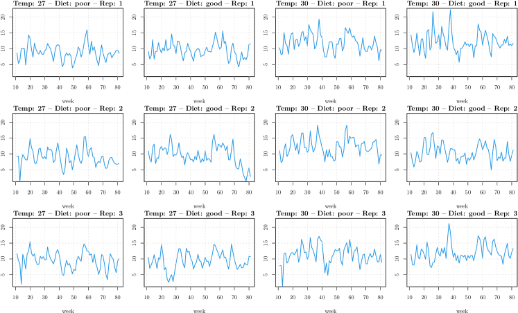
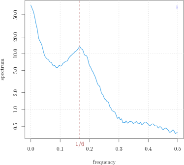
Refer to caption
Figure 5: Time series of 12 populations of P. interpunctella from week 11 to 82 for different experimental conditions. The series have been square-root transformed.
Refer to caption
Refer to caption
Figure 6: (Left) Power spectral density of the simulated time series of 100k observations from the model fit of the first time series (temp: 27°, diet: poor). The frequency corresponding to the characteristic 6-week cycle is evidenced with a vertical dashed line.(Right) Histogram of the data (yellow) with the superimposed density of the fitted model, estimated upon the simulated series (blue line).
Refer to caption
Refer to caption
Figure 7: (Left) Power spectral density of the simulated time series of 100k observations from the model fit of the third time series (temp: 30°, diet: poor). The frequency corresponding to the characteristic 6-week cycle is evidenced with a vertical dashed line.(Right) Histogram of the data (yellow) with the superimposed density of the fitted model, estimated upon the simulated series (blue line).
Refer to caption
Refer to caption
Figure 8: (Left) Power spectral density of the simulated time series of 100k observations from the model fit of the third time series (temp: 30°, diet: poor). The frequency corresponding to the characteristic 6-week cycle is evidenced with a vertical dashed line.(Right) Histogram of the data (yellow) with the superimposed density of the fitted model, estimated upon the simulated series (blue line).
Refer to caption
Refer to caption
Refer to caption
Refer to caption
Figure 9: Temperature: 27° - Diet: poor. Correlograms of the residuals of the TARMA model of Eq. (29). Autocorrelation function (left) and partial autocorrelation function (right). The blue dashed lines indicate the rejection bands at 99% level.
Refer to caption
Refer to caption
Refer to caption
Refer to caption
Figure 10: Temperature: 27° - Diet: good. Correlograms of the residuals of the TARMA model of Eq. (29). Autocorrelation function (left) and partial autocorrelation function (right). The blue dashed lines indicate the rejection bands at 99% level.
Refer to caption
Refer to caption
Refer to caption
Refer to caption
Figure 11: Temperature: 30° - Diet: poor. Correlograms of the residuals of the TARMA model of Eq. (29). Autocorrelation function (left) and partial autocorrelation function (right). The blue dashed lines indicate the rejection bands at 99% level.
Refer to caption
Refer to caption
Refer to caption
Refer to caption
Figure 12: Temperature: 30° - Diet: good. Correlograms of the residuals of the TARMA model of Eq. (29). Autocorrelation function (left) and partial autocorrelation function (right). The blue dashed lines indicate the rejection bands at 99% level.
temp. diet W p-value
27 poor 0.989 0.849
27 good 0.984 0.578
30 poor 0.987 0.730
30 good 0.963 0.046
Table 2: Shapiro Wilk normality test statistic and p𝑝p-values for the residuals of the fitted threshold ARMA models.