High-pressure hydrogen by machine learning and quantum Monte Carlo
Abstract
We have developed a technique combining the accuracy of quantum Monte Carlo in describing the electron correlation with the efficiency of a Machine Learning Potential (MLP). We use kernel regression in combination with SOAP (Smooth Overlap of Atomic Position) features, implemented here in a very efficient way. The key ingredients are: i) a sparsification technique, based on farthest point sampling, ensuring generality and transferability of our MLPs and ii) the so called -learning, allowing a small training data set, a fundamental property for highly accurate but computationally demanding calculations, such as the ones based on quantum Monte Carlo. As the first application we present a benchmark study of the liquid-liquid transition of high-pressure hydrogen and show the quality of our MLP, by emphasizing the importance of high accuracy for this very debated subject, where experiments are difficult in the lab, and theory is still far from being conclusive.
Introduction. The determination of the phase diagram of hydrogen at high pressure has been a particularly long-standing problem in the physics community since the pioneering work of Wigner and Huntington [1]. Recently it has received renewed interest, e.g., for the still controversial properties of the newly discovered H-based superconductors such as H3S [2] and LaH10 [3] , for establishing the polymorphs of the solid phase of hydrogen [4, 5] and, last but not least, for characterizing the nature of the liquid-liquid transition (LLT) between molecular and atomic phases.
In this work we are mainly addressing the last aspect,
that is of paramount importance for determining the composition of giant planets, and, by consequence, of our universe.
Unfortunately, many contradictory experimental [6, 7, 8, 9, 10, 11] and computational [12, 13, 14, 15, 16, 17, 18, 19] results have been reported so far, about whether the LLT is a first-order or a smooth transition, and the location of the LLT on the - phase diagram.
Indeed, for studying phase transition phenomena, molecular dynamics simulations with long times and several atoms are required, in order to exclude equilibration and finite-size effect artifacts, respectively.
In this respect, the construction of Machine Learning Potentials (MLPs), aimed to
reproduce accurate electronic energies and force fields, is one of the most promising approaches to overcome the large computational cost of present ab-initio techniques for electronic simulation [20]. In fact, very recently, Cheng et al. [19] constructed MLPs for hydrogen, using the Behler–Parrinello artificial Neural Network framework (NNPs) [21, 22] based on Density Functional Theory (DFT) references.
Here we show that this approach can be extended to a state-of-the-art
wave function method, quantum Monte Carlo (QMC) [23], that is well known to describe very accurately the electronic correlation but has a computational cost
at least three orders of magnitude larger than DFT.
Indeed in hydrogen, it is important to have a very reliable technique,
because experiments are difficult at extreme conditions and DFT, on the other hand, depends too much on the functional used [24, 25].
In this letter we aim to produce a MLP
that is efficient enough to allow long and large size simulations, but on the other hand, retains the same accuracy of QMC, and, importantly, the training can be achieved by a relatively small number of simulations.
We will show that this is possible, by employing the -learning method combined with the Gaussian Kernel Regression (GKR) framework [26].
Model and methods.
We outline the theoretical and technical details of the Machine Learning (ML) models that can be trained using our algorithmic approach.
SOAP kernel method.
One of the key features of modern MLPs is their applicability to systems with an arbitrary number of atoms , allowing simulations with sizes much larger than the ones used during the training. One possibility is to write the total energy of the system as a sum of contributions depending on the local environment around each atom placed at the position [21], where . The function depends only on the neighbors of atom inside a sphere with radius , namely such that ().
Several approaches are possible to parametrize . In this work we used a kernel regression model
| (1) |
where is the normalized kernel between two local environments (the target one) and (the ones used for the training, that may or may not contain ), and are coefficients to be determined. Here is the total number of local environments used for the construction of the MLP.
The local environment around each atom is characterized using the Smooth Overlap of Atomic Positions (SOAP), [27]: in such an approach, a density function is associated to each local environment . Hence:
where is a cutoff function and is a hyper-parameter of the model. In this work a piece-wise defined polynomial, vanishing smoothly at , was used as 111 if and for . We also assume that , in order to exclude the trivial contribution.. The similarity kernel between two local environments and is defined as the average over all rotations of the overlap between the densities raised to some exponent :
| (2) |
With this definition the resulting kernel is explicitly invariant under permutation of the particles and rotations in 3D space. In order to compute the integral in Eq. (2), the usual approach is to expand in radial and angular components and evaluate the power spectrum [27]. Here instead, in analogy with the nowadays standard implementation of non local pseudopotentials within QMC [29] (where a similar angular integration appears), we have used an approximate version of Eq. (2) which takes the average of the overlap only over a finite subgroup (e.g. all the symmetries of the cube) of , that is spanned by real orthogonal matrices :
| (3) |
The resulting kernel is explicitly invariant under the set of transformations considered, that approaches the full continuous symmetry
for large .
Just like for QMC pseudopotential calculations, we have experienced that a relatively small is sufficient to reach the desired accuracy.
Moreover Eq. (3) can be computed in a very efficient way since each term in the sum has a simple expression in terms of Gaussian functions.
Finally, in order to obtain in Eq. (1), we normalize and raise it to some power , so that .
Local sparsification. A key aspect in the implementation and training of a ML model is the prevention of overfitting, i.e. the statistical phenomenon for which a model can fit almost exactly the training data but fails to predict unknown data reliably.
Overfitting problems can arise when the number of variational parameters of a given model is too large. Moreover, since the number of variational parameters in a GKR model depends linearly on the size of the training set, particular care should be taken when selecting the corresponding reference samples. This becomes even more important in the present setting: indeed, adding one configuration with atoms to the training dataset implicitly defines new local environments corresponding to further variational degrees of freedom of the model in Eq. (1). Additionally, the computational effort needed in the training of a GKR model is polynomial (at most cubic) in the size of the training set – while instead stochastic optimization algorithms employed in neural networks allow the complexity to be independent of the size of the number of samples.
Therefore, within GKR, the careful choice of the local environments used in the training phase is of paramount importance. This is usually obtained by means of the so called sparsification. We implement a variant of it, that we name local sparsification, since we discard from each configuration some or even a large fraction of the corresponding local environments. This prevents overfitting and allows an increased predictive power of the model on unseen data.
The local sparsification preprocessing can be performed with multiple algorithms, and we employ the farthest point sampling scheme, which is a greedy algorithm first adopted as an approximate solution of the so-called Center Selection Problem (see [30, §11.2]).
A detailed explanation of our algorithm is contained in the Supplementary Material.
-machine learning. In this work we also follow the -Machine Learning (-ML) approach, first introduced in Ref. 31 as a composite strategy reproducing a target ab-initio method, by adding ML corrections to a much cheaper baseline reference potential. Here, we take as baseline ab-initio reference a DFT calculation with PBE functional and as target method Variational Monte Carlo (VMC).
There is a significant gain in exploiting the -ML approach: by training on the difference between two ab-initio methods, the machine learning task becomes easier. This is crucial for the case at hand: if we were to train a GKR model to predict VMC observables, the amount of training configurations to achieve the desired accuracy would require a computational effort which is at present not feasible. In particular, we are able to obtain a VMC potential with an accuracy comparable with the error bar of the VMC predictions, by training the model on a relatively small dataset. Moreover, the computational cost of the ML inference (also thanks to the local sparsification preprocessing) is negligible compared to the baseline DFT calculation. Hence, we are able to compute observables with VMC accuracy at the cost of a DFT simulation.
Results.
We discuss now the first successful application of our method to the study of the LLT in hydrogen at high pressures. Our dataset is composed of configurations of hydrogen atoms in cubic simulation cells of different edge sizes, from to bohr.
For each of these configurations we computed the ground state energy, the force components acting on each atom and the pressure of the system using two different ab-initio methods: DFT with the PBE and BLYP functionals, with the Quantum Espresso software package, [32]; VMC, with the TurboRVB software package, [33]. Concerning the VMC simulations, the predicted energies, force components and pressure have average error bars of Ha, Ha/Bohr and GPa, respectively. Note that performing a molecular dynamics (MD) simulation using VMC with such an accuracy at each step would be computationally prohibitive.
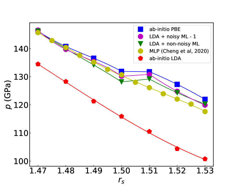
Performances of the -ML correction. Although computing the root mean square error (RMSE) on target quantities is a standard approach to access the predictive power of a ML model, it seems necessary in our case to have more tailored qualitative and quantitative performance metrics. Since QMC provides training data with intrinsic noise, the first step in our study is to determine how this affects the ML approach. To this purpose, since it is not possible to have an unbiased –i.e. noiseless– VMC reference, we have performed the following test: we trained our GKR on two datasets, such that one was simply the difference between a DFT baseline reference (calculated with the LDA functional) and a DFT-PBE target, while the other was a noisy version of the first, where we introduced Gaussian white noises on the observables in order to emulate QMC inputs. As shown in Fig. 1(a) the effect of a noise a.u. on forces and total energies 222This error bar can be achieved for instance by a single QMC simulation on about one thousand processors for about a couple of hours within the TurboRVB package [33]. Clearly this error bar cannot be sustained for an MD run with several thousands steps, as the ones employed here. is almost negligible, yielding a pressure plateau almost indistinguishable from the reference PBE one and the MLP trained with the noiseless data set. The performances of the proposed MLP are also much better than the ones of the previous attempt [19], unable to reproduce the pressure plateau in this case. This is remarkable because in this region the LDA baseline is very far from the reference and also featureless. Note also that our finding is compatible with Fig. S6 of Ref. 19, since in that graph the grid employed for the Ab-initio Molecular Dynamics (AIMD) PBE simulations is very coarse and away from the plateau.
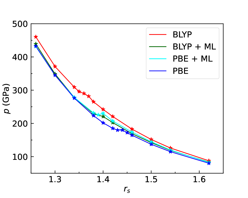
Given this remarkable stability property of our GKR against noise, we further show the independence of the method (see Fig. 1(b)) when trained 1) with true QMC noisy data
and 2) starting from two references, namely PBE and BLYP.
As shown in Fig. 1(b),
we have obtained an excellent agreement between the two MLP EOS, even though the two DFT-based isotherms differ significantly from each other. In particular the transition pressure changes by almost GPa with the two chosen DFT functionals. Nevertheless the two models corrected with the MLP are much closer, with a difference in the predicted not larger than GPa (or anyway within the error bars) in the range of densities explored.
For the rest of this work, we used the PBE-DFT method as our baseline potential, since it appears to provide results closer to the VMC ones.
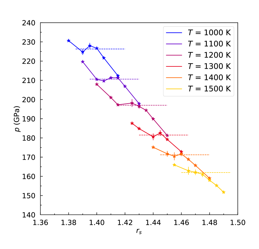
LLT for high-pressure hydrogen. We have considered two systems of 128 and 256 hydrogen atoms respectively and performed a series of classical NVT simulations for several values of the density and temperature. At each step of MD we first compute DFT-PBE forces for the given configuration and then sum the correction given by our MLP. We have used a time step of 10 a.u. (i.e. 0.242 fs) and controlled the temperature using either second order Langevin dynamics [35] or a Bussi-Parrinello thermostat [36]. A cubic supercell has been considered for all the simulations. For each point we have chosen a time simulation length between 2 ps and 10 ps, from which we have calculated the average of the thermodynamic quantities of interest. We remark that, even though our -ML approach is still expensive (it has the same cost of a standard DFT Born-Oppenheimer MD), it is about times faster than computing directly VMC forces at each step, with the chosen accuracy.
For all cases considered we have found a narrow but clear plateau, suggesting a first order nature of the LLT transition in this system (Fig. 2(a)). Both the transition pressures and corresponding densities are quantitatively much different from the DFT ones, suggesting the importance of the VMC correction for the accurate evaluation of those quantities.
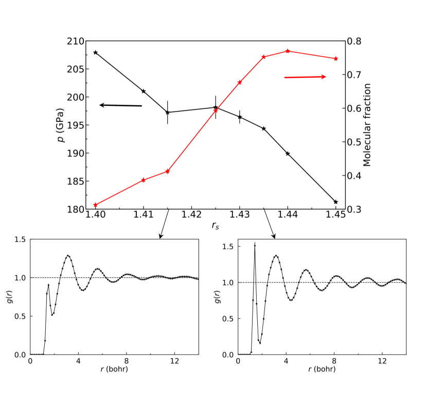
We have also computed the average of the molecular fraction along the trajectory, defined as the percentage of atoms with at least one neighbor inside a cutoff of a.u., i.e.
where is a cutoff function that is equal to for a.u. and goes smoothly to for a.u.
As evident in Fig. (2(b)), at the location of the pressure plateau the molecular fraction jumps from small values, corresponding to an atomic liquid, to values closer to , typical for a molecular system. This can be also noticed by computing the radial distribution function for two values of the density at opposite sides of the transition.
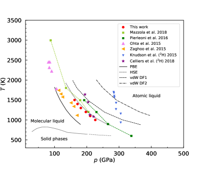
In Fig. (3) we report the computed transition line, alongside with previous numerical and experimental results. As expected, we have found good agreement with previous VMC based molecular dynamics simulations that used the same wave function [17] but the statistical error on energy, forces and pressure were an order of magnitude larger, thus explaining the small differences found. Our calculations give transition pressures that are 30 GPa below the ones predicted by the CEIMC method [37]. The reason of this discrepancy is not clear at present; in principle the calculations done in Ref. 37 could be more accurate due to the presence of backflow correlation and Diffusion Monte Carlo (DMC) projection, that could be further included for the training of our MLP. However, from our benchmark tests DMC gives only a small correction to the VMC forces, that is compatible with the error bars as shown in the Supplementary Material. Our results are also in excellent agreement with the Diamond Anvil Cell (DAC) experiments of Refs. 8 and 10, especially if we take into account that quantum corrections tend to further lower the transition pressure.
We conclude this discussion by pointing out that our method gives almost the same line as the hybrid HSE functional. This could be useful for future studies based on DFT for high pressure hydrogen.
Conclusion.
In this work we have introduced a successful approach, combining the ML and QMC techniques: in particular, through the -ML framework, we are able to obtain energies, forces and pressure predictions with QMC accuracy, at a computational cost comparable to DFT, allowing simulations that were previously impossible (see SI Fig. S7, where MD simulations with , at the QMC accuracy, are shown). Our technique is perfectly suited for being employed in a context where high accuracy is needed, but small training data sets are available.
We benchmarked our approach by studying the LLT in hydrogen at high pressures, whose phase diagram has been under a very lively debate, especially recently. In this context, our method is capable
of reproducing the pressure plateau computed directly with PBE at 1400K, in contrast to the previously proposed NN MLP. This outcome appears in agreement with Ref. 39 but the subtle question whether a genuine first order transition or a sharp crossover occurs, is outside the scope of this letter, and will be dealt with in future works with much larger and simulation times. Moreover
we believe that further substantial improvements will be possible by using
baseline potentials (e.g. the recent ultrafast MLP [40]) much more efficient than DFT ones.
Indeed,
we expect that our approach will enable the study of systems that have been so far impossible to simulate, due to the almost intractable computational cost required by advanced many-body techniques, such as QMC.
Acknowledgments. We thank Matthias Rupp for useful discussions and careful reading of the manuscript. The computations in this work have been mainly performed using the supercomputer Fugaku provided by RIKEN through the HPCI System Research Project (Project ID: hp210038) and Marconi100 provided by CINECA through the PRACE project No. 2019204934 and ISCRA project AI-H-QMC, HP10BGJH1X. K.N. is also grateful for computational resources from the facilities of Research Center for Advanced Computing Infrastructure at Japan Advanced Institute of Science and Technology (JAIST). A.T. and S.S. acknowledge financial support from the MIUR Progetti di Ricerca di Rilevante Interesse Nazionale (PRIN) Bando 2017 - grant 2017BZPKSZ. K.N. acknowledges a support from the JSPS Overseas Research Fellowships, that from Grant-in-Aid for Early-Career Scientists Grant Number JP21K17752, and that from Grant-in-Aid for Scientific Research(C) Grant Number JP21K03400. This work is supported by the European Centre of Excellence in Exascale Computing TREX - Targeting Real Chemical Accuracy at the Exascale. This project has received funding from the European Union’s Horizon 2020 - Research and Innovation program - under grant agreement no. 952165.
References
- Wigner and Huntington [1935] E. Wigner and H. Huntington, J. Chem. Phys. 3, 764 (1935).
- Drozdov et al. [2015] A. Drozdov, M. Eremets, I. Troyan, V. Ksenofontov, and S. I. Shylin, Nature 525, 73 (2015).
- Somayazulu et al. [2019] M. Somayazulu, M. Ahart, A. K. Mishra, Z. M. Geballe, M. Baldini, Y. Meng, V. V. Struzhkin, and R. J. Hemley, Phys. Rev. Lett. 122, 027001 (2019).
- Drummond et al. [2015] N. D. Drummond, B. Monserrat, J. H. Lloyd-Williams, P. L. Ríos, C. J. Pickard, and R. J. Needs, Nat. Commun. 6, 1 (2015).
- Drozdov et al. [2019] A. Drozdov, P. Kong, V. Minkov, S. Besedin, M. Kuzovnikov, S. Mozaffari, L. Balicas, F. Balakirev, D. Graf, V. Prakapenka, et al., Nature 569, 528 (2019).
- Celliers et al. [2018] P. M. Celliers, M. Millot, S. Brygoo, R. S. McWilliams, D. E. Fratanduono, J. R. Rygg, A. F. Goncharov, P. Loubeyre, J. H. Eggert, J. L. Peterson, et al., Science 361, 677 (2018).
- Knudson et al. [2015] M. D. Knudson, M. P. Desjarlais, A. Becker, R. W. Lemke, K. Cochrane, M. E. Savage, D. E. Bliss, T. Mattsson, and R. Redmer, Science 348, 1455 (2015).
- Ohta et al. [2015] K. Ohta, K. Ichimaru, M. Einaga, S. Kawaguchi, K. Shimizu, T. Matsuoka, N. Hirao, and Y. Ohishi, Sci. Rep. 5, 1 (2015).
- McWilliams et al. [2016] R. S. McWilliams, D. A. Dalton, M. F. Mahmood, and A. F. Goncharov, Phys. Rev. Lett. 116, 255501 (2016).
- Zaghoo et al. [2016] M. Zaghoo, A. Salamat, and I. F. Silvera, Phys. Rev. B 93, 155128 (2016).
- Zaghoo and Silvera [2017] M. Zaghoo and I. F. Silvera, Proc. Natl. Acad. Sci. U.S.A. 114, 11873 (2017).
- Scandolo [2003] S. Scandolo, Proc. Natl. Acad. Sci. U.S.A. 100, 3051 (2003).
- Morales et al. [2010] M. A. Morales, C. Pierleoni, E. Schwegler, and D. M. Ceperley, Proc. Natl. Acad. Sci. U.S.A. 107, 12799 (2010).
- Lorenzen et al. [2010] W. Lorenzen, B. Holst, and R. Redmer, Phys. Rev. B 82, 195107 (2010).
- Delaney et al. [2006] K. T. Delaney, C. Pierleoni, and D. Ceperley, Phys. Rev. Lett. 97, 235702 (2006).
- Vorberger et al. [2007] J. Vorberger, I. Tamblyn, B. Militzer, and S. Bonev, Phys. Rev. B 75, 024206 (2007).
- Mazzola et al. [2018] G. Mazzola, R. Helled, and S. Sorella, Phys. Rev. Lett. 120, 025701 (2018).
- Geng et al. [2019] H. Y. Geng, Q. Wu, M. Marqués, and G. J. Ackland, Phys. Rev. B 100, 134109 (2019).
- Cheng et al. [2020] B. Cheng, G. Mazzola, C. J. Pickard, and M. Ceriotti, Nature 585, 217 (2020).
- Jia et al. [2020] W. Jia, H. Wang, M. Chen, D. Lu, L. Lin, R. Car, W. E, and L. Zhang, Pushing the limit of molecular dynamics with ab initio accuracy to 100 million atoms with machine learning, in Proceedings of the International Conference for High Performance Computing, Networking, Storage and Analysis (IEEE Press, 2020).
- Behler and Parrinello [2007] J. Behler and M. Parrinello, Phys. Rev. Lett. 98, 146401 (2007).
- Behler [2011] J. Behler, J. Chem. Phys. 134, 074106 (2011).
- Foulkes et al. [2001] W. Foulkes, L. Mitas, R. Needs, and G. Rajagopal, Rev. Mod. Phys. 73, 33 (2001).
- Azadi and Foulkes [2013] S. Azadi and W. M. C. Foulkes, Phys. Rev. B 88, 014115 (2013).
- Clay et al. [2014] R. C. Clay, J. Mcminis, J. M. McMahon, C. Pierleoni, D. M. Ceperley, and M. A. Morales, Phys. Rev. B 89, 184106 (2014).
- Bartók et al. [2010] A. P. Bartók, M. C. Payne, R. Kondor, and G. Csányi, Phys. Rev. Lett. 104, 136403 (2010).
- Bartók et al. [2013] A. P. Bartók, R. Kondor, and G. Csányi, Phys. Rev. B 87, 184115 (2013).
- Note [1] if and for . We also assume that , in order to exclude the trivial contribution.
- Mitáš et al. [1991] L. Mitáš, E. L. Shirley, and D. M. Ceperley, J. Chem. Phys. 95, 3467 (1991).
- Kleinberg and Tardos [2006] J. Kleinberg and E. Tardos, Algorithm design (Pearson Education India, 2006).
- Ramakrishnan et al. [2015] R. Ramakrishnan, P. O. Dral, M. Rupp, and O. A. von Lilienfeld, J. Chem. Theory Comput. 11, 2087 (2015).
- Giannozzi et al. [2009] P. Giannozzi, S. Baroni, N. Bonini, M. Calandra, R. Car, C. Cavazzoni, D. Ceresoli, G. L. Chiarotti, M. Cococcioni, I. Dabo, et al., J. Phys. Condens. Matter. 21, 395502 (2009).
- Nakano et al. [2020] K. Nakano, C. Attaccalite, M. Barborini, L. Capriotti, M. Casula, E. Coccia, M. Dagrada, C. Genovese, Y. Luo, G. Mazzola, A. Zen, and S. Sorella, J. Chem. Phys. 152, 204121 (2020).
- Note [2] This error bar can be achieved for instance by a single QMC simulation on about one thousand processors for about a couple of hours within the TurboRVB package [33]. Clearly this error bar cannot be sustained for an MD run with several thousands steps, as the ones employed here.
- Kampen [2007] N. V. Kampen, in Stochastic Processes in Physics and Chemistry (Third Edition), North-Holland Personal Library, edited by N. Van Kampen (Elsevier, Amsterdam, 2007) third edition ed., pp. 219–243.
- Bussi et al. [2007] G. Bussi, D. Donadio, and M. Parrinello, J. Chem. Phys. 126, 014101 (2007).
- Pierleoni et al. [2016] C. Pierleoni, M. A. Morales, G. Rillo, M. Holzmann, and D. M. Ceperley, Proc. Natl. Acad. Sci. U.S.A. 113, 4953 (2016).
- Rohatgi [2021] A. Rohatgi, Webplotdigitizer: Version 4.5, https://automeris.io/WebPlotDigitizer (2021).
- Karasiev et al. [2021] V. V. Karasiev, J. Hinz, S. X. Hu, and S. B. Trickey, Nature 600, E12 (2021).
- Xie et al. [2021] S. R. Xie, M. Rupp, and R. G. Hennig, Ultra-fast interpretable machine-learning potentials (2021), arXiv:2110.00624 [cond-mat.mtrl-sci] .