ICON: Implicit Clothed humans Obtained from Normals

Abstract

Current methods for learning realistic and animatable 3D clothed avatars need either posed 3D scans or 2D images with carefully controlled user poses. In contrast, our goal is to learn an avatar from only 2D images of people in unconstrained poses. Given a set of images, our method estimates a detailed 3D surface from each image and then combines these into an animatable avatar. Implicit functions are well suited to the first task, as they can capture details like hair and clothes. Current methods, however, are not robust to varied human poses and often produce 3D surfaces with broken or disembodied limbs, missing details, or non-human shapes. The problem is that these methods use global feature encoders that are sensitive to global pose. To address this, we propose ICON (“Implicit Clothed humans Obtained from Normals”), which, instead, uses local features. ICON has two main modules, both of which exploit the SMPL(-X) body model. First, ICON infers detailed clothed-human normals (front/back) conditioned on the SMPL(-X) normals. Second, a visibility-aware implicit surface regressor produces an iso-surface of a human occupancy field. Importantly, at inference time, a feedback loop alternates between refining the SMPL(-X) mesh using the inferred clothed normals and then refining the normals. Given multiple reconstructed frames of a subject in varied poses, we use a modified version of SCANimate to produce an animatable avatar from them. Evaluation on the AGORA and CAPE datasets shows that ICON outperforms the state of the art in reconstruction, even with heavily limited training data. Additionally, it is much more robust to out-of-distribution samples, e.g., in-the-wild poses/images and out-of-frame cropping. ICON takes a step towards robust 3D clothed human reconstruction from in-the-wild images. This enables avatar creation directly from video with personalized pose-dependent cloth deformation. Models and code are available for research at https://icon.is.tue.mpg.de.

1 Introduction

Realistic virtual humans will play a central role in mixed and augmented reality, forming a key foundation for the “metaverse” and supporting remote presence, collaboration, education, and entertainment. To enable this, new tools are needed to easily create 3D virtual humans that can be readily animated. Traditionally, this requires significant artist effort and expensive scanning equipment. Therefore, such approaches do not scale easily. A more practical approach would enable individuals to create an avatar from one or more images. There are now several methods that take a single image and regress a minimally clothed 3D human model [21, 48, 33, 6, 7, 18]. Existing parametric body models, however, lack important details like clothing and hair [29, 38, 48, 53, 64]. In contrast, we present a method that robustly extracts 3D scan-like data from images of people in arbitrary poses and uses this to construct an animatable avatar.

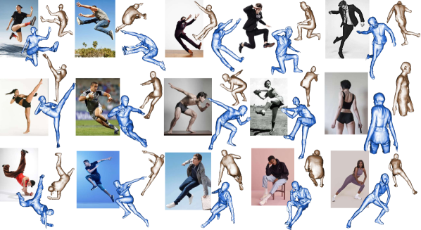
We base our approach on implicit functions (IFs), which go beyond parametric body models to represent fine shape details and varied topology. IFs allow recent methods to infer detailed shape from an image [54, 55, 70, 24, 22, 65]. Despite promising results, state-of-the-art  (SOTA) methods struggle with in-the-wild data and often produce humans with broken or disembodied limbs, missing details, high-frequency noise, or non-human shape; see Fig. 2 for examples.

The issues with previous methods are twofold: (1) Such methods are typically trained on small, hand-curated, 3D human datasets (e.g. Renderpeople [3]) with very limited pose, shape and clothing variation. (2) They typically feed their implicit-function module with features of a global 2D image or 3D voxel encoder, but these are sensitive to global pose. While more, and more varied, 3D training data would help, such data remains limited. Hence, we take a different approach and improve the model.

Specifically, our goal is to reconstruct a detailed clothed 3D human from a single RGB image with a method that is training-data efficient and robust to in-the-wild images and out-of-distribution poses. Our method, called ICON, stands for Implicit Clothed humans Obtained from Normals. ICON replaces the global encoder of existing methods with a more data-efficient local scheme; Fig. 3 shows a model overview. ICON takes as input an RGB image of a segmented clothed human and a SMPL body estimated from the image [32]. The SMPL body is used to guide two of ICON’s modules: one infers detailed clothed-human surface normals (front and back views), and the other infers a visibility-aware implicit surface (iso-surface of an occupancy field). Errors in the initial SMPL estimate, however, might misguide inference. Thus, at inference time, an iterative feedback loop refines SMPL (i.e., its 3D shape, pose, and translation) using the inferred detailed normals, and vice versa, leading to a refined implicit shape with better 3D details.

Figure 2: SOTA methods for inferring 3D humans from in-the-wild images, e.g., PIFu, PIFuHD, PaMIR, and ARCH++, struggle with challenging poses and out-of-frame cropping (E), resulting in various artifacts including non-human shapes (A,G), disembodied parts (B,H), missing body parts (C,D), missing details (E), and high-frequency noise (F). ICON deals with these challenges and produces high-quality results, highlighted with a green shadow Front view (blue) and rotated view (bronze).

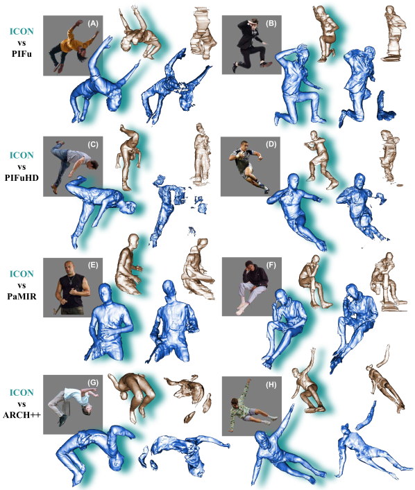
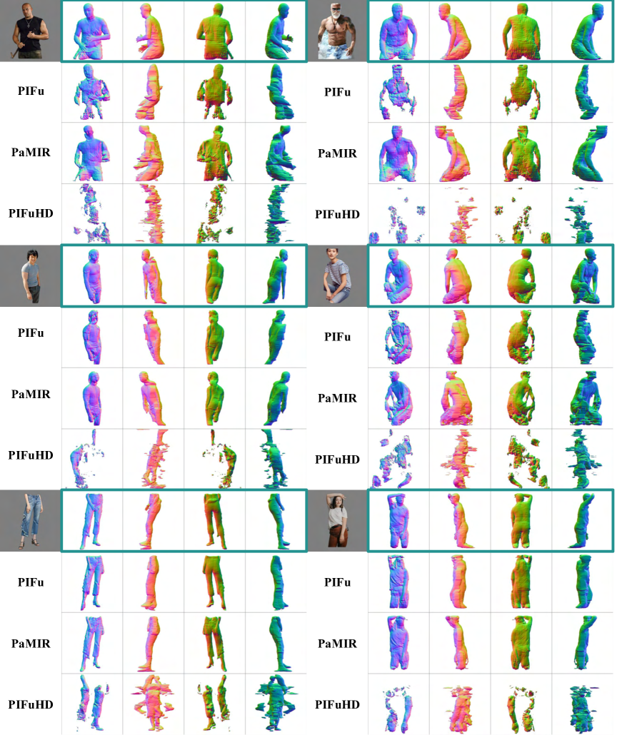
We evaluate ICON quantitatively and qualitatively on challenging datasets, namely AGORA [47] and CAPE [41], as well as on in-the-wild images. Results show that ICON has two advantages w.r.t. the state of the art: (1) Generalization. ICON’s locality helps it generalize to in-the-wild images and out-of-distribution poses and clothes better than previous methods. Representative cases are shown in Fig. 2; notice that, although ICON is trained on full-body images only, it can handle images with out-of-frame cropping, with no fine tuning or post processing. (2) Data efficacy. ICON’s locality helps it avoid spurious correlations between pose and surface shape. Thus, it needs less data for training. ICON significantly outperforms baselines in low-data regimes, as it reaches SOTA performance when trained with as little as $12\%$ of the data.

We provide an example application of ICON for creating an animatable avatar; see ICON: Implicit Clothed humans Obtained from Normals for an overview. We first apply ICON on the individual frames of a video sequence, to obtain 3D meshes of a clothed person in various poses. We then use these to train a poseable avatar using a modified version of SCANimate [56]. Unlike 3D scans, which SCANimate takes as input, our estimated shapes are not equally detailed and reliable from all views. Consequently, we modify SCANimate to exploit visibility information in learning the avatar. The output is a 3D clothed avatar that moves and deforms naturally; see ICON: Implicit Clothed humans Obtained from Normals-right and Fig. 7(b).

ICON takes a step towards robust reconstruction of 3D clothed humans from in-the-wild photos. Based on this, fully textured and animatable avatars with personalized pose-aware clothing deformation can be created directly from video frames. Models and code are available at https://icon.is.tue.mpg.de.

2 Related work

Mesh-based statistical models. Mesh-based statistical body models [29, 38, 48, 53, 64] are a popular explicit representation for 3D human reconstruction. This is not only because such models capture the statistics across a human population, but also because meshes are compatible with standard graphics pipelines. A lot of work [30, 33, 31, 66, 58, 57, 18] estimates 3D body meshes from an RGB image, but these have no clothing. Other work estimates clothed humans, instead, by modeling clothing geometry as 3D offsets on top of body geometry [6, 5, 4, 72, 34, 50, 7, 63]. The resulting clothed 3D humans can be easily animated, as they naturally inherit the skeleton and surface skinning weights from the underlying body model. An important limitation, though, is modeling clothing such as skirts and dresses; since these differ a lot from the body surface, simple body-to-cloth offsets are insufficient. To address this, some methods [12, 27] use a classifier to identify cloth types in the input image, and then perform cloth-aware inference for 3D reconstruction. However, such a remedy does not scale up to a large variety of clothing types. Another advantage of mesh-based statistical models, is that texture information can be easily accumulated through multi-view images or image sequences [6, 12], due to their consistent mesh topology. The biggest limitation, though, is that the state of the art does not generalize well w.r.t. clothing-type variation, and it estimates meshes that do not align well to input-image pixels.

Deep implicit functions. Unlike meshes, deep implicit functions [46, 44, 17] can represent detailed 3D shapes with arbitrary topology, and have no resolution limitations. Saito et al. [54] introduce deep implicit functions for clothed 3D human reconstruction from RGB images and, later [55], they significantly improve 3D geometric details. The estimated shapes align well to image pixels. However, their shape reconstruction lacks regularization, and often produces artifacts like broken or disembodied limbs, missing details, or geometric noise. He et al. [22] add a coarse-occupancy prediction branch, and Li et al. [37] and Dong et al. [20] use depth information captured by an RGB-D camera to further regularize shape estimation and provide robustness to pose variation. Li et al. [36, 35] speed up inference through an efficient volumetric sampling scheme. A limitation of all above methods is that the estimated 3D humans cannot be reposed, because implicit shapes (unlike statistical models) lack a consistent mesh topology, a skeleton, and skinning weights. To address this, Bozic et al. [14] infer an embedded deformation graph to manipulate implicit functions, while Yang et al. [65] also infer a skeleton and skinning fields.

Statistical models & implicit functions. Mesh-based statistical models are well regularized, while deep implicit functions are much more expressive. To get the best of both worlds, recent methods [10, 24, 11, 70] combine the two representations. Given a sparse point cloud of a clothed person, IPNet [10] infers an occupancy field with body/clothing layers, registers SMPL to the body layer with inferred body-part segmentation, and captures clothing as offsets from SMPL to the point cloud. Given an RGB image of a clothed person, ARCH [24] and ARCH++ [23] reconstruct 3D human shape in a canonical space by warping query points from the canonical to the posed space, and projecting them onto the 2D image space. However, to train these models, one needs to unpose scans into the canonical pose with an accurately fitted body model; inaccurate poses cause artifacts. Moreover, unposing clothed scans using the “undressed” model’s skinning weights alters shape details. For the same RGB input, Zheng et al. [70, 69] condition the implicit function on a posed and voxelized SMPL mesh for robustness to pose variation and reconstruct local details from the image pixels, similar to PIFu [54]. However, these methods are sensitive to global pose, due to their 3D convolutional encoder. Thus, for training data with limited pose variation, they struggle with out-of-distribution poses and in-the-wild images.

Positioning ICON w.r.t. related work. ICON combines the statistical body model SMPL with an implicit function, to reconstruct clothed 3D human shape from a single RGB image. SMPL not only guides ICON’s estimation, but is also optimized “in the loop” during inference to enhance its pose accuracy. Instead of relying on the global body features, ICON exploits local body features that are agnostic to global pose variations. As a result, even when trained on heavily limited data, ICON achieves state-of-the-art performance and is robust to out-of-distribution poses. This work links monocular 3D clothed human reconstruction to scan/depth based avatar modeling algorithms [56, 62, 16, 60, 19, 40, 42].

3 Method

Figure 3: ICON’s architecture contains two main modules for: (1) body-guided normal prediction, and (2) local-feature based implicit 3D reconstruction. The dotted line with an arrow is a 2D or 3D query function. The two $\mathcal{G}^{\text{N}}$ networks (purple/orange) have different parameters.

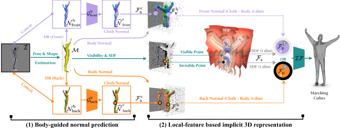
ICON is a deep-learning model that infers a 3D clothed human from a color image. Specifically, ICON takes as input an RGB image with a segmented clothed human (following the suggestion of PIFuHD’s repository [49]), along with an estimated human body shape “under clothing” (SMPL), and outputs a pixel-aligned 3D shape reconstruction of the clothed human. ICON has two main modules (see Fig. 3) for: (1) SMPL-guided clothed-body normal prediction and (2) local-feature based implicit surface reconstruction.

3.1 Body-guided normal prediction

Inferring full-$360^{\circ}$ 3D normals from a single RGB image of a clothed person is challenging; normals for the occluded parts need to be hallucinated based on the observed parts. This is an ill-posed task and is challenging for deep networks. Unlike model-free methods [26, 55, 59], ICON takes into account a SMPL [38] “body-under-clothing” mesh to reduce ambiguities and guide front and (especially) back clothed -body normal prediction. To estimate the SMPL mesh $\mathcal{M}(\beta,\theta)\in\mathbb{R}^{N\times 3}$ from image $\mathcal{I}$, we use PyMAF [68] due to its better mesh-to-image alignment compared to other methods. SMPL is parameterized by shape, $\beta\in\mathbb{R}^{10}$, and pose, $\theta\in\mathbb{R}^{3\times K}$, where $N=6,890$ vertices and $K=24$ joints. ICON is also compatible with SMPL-X [48].

Under a weak-perspective camera model, with scale $s\in\mathbb{R}$ and translation $t\in\mathbb{R}^{3}$, we use the PyTorch3D [51] differentiable renderer, denoted as $\mathcal{DR}$, to render $\mathcal{M}$ from two opposite views, obtaining “front” (i.e., observable side) and “back” (i.e., occluded side) SMPL-body normal maps $\mathcal{N}^{\text{b}}=\{\mathcal{N}^{\text{b}}_{\text{front}},\mathcal{N}^{\text{b}}_{\text{back}}\}$. Given $\mathcal{N}^{\text{b}}$ and the original color image $\mathcal{I}$, our normal networks $\mathcal{G}^{\text{N}}=\{\mathcal{G}^{\text{N}}_{\text{front}},\mathcal{G}^{\text{N}}_{\text{back}}\}$ predict clothed-body normal maps, denoted as $\widehat{\mathcal{N}}^{\text{c}}=\{\widehat{\mathcal{N}}^{\text{c}}_{\text{front}},\widehat{\mathcal{N}}^{\text{c}}_{\text{back}}\}$:

$$\mathcal{DR}(\mathcal{M}) \rightarrow\mathcal{N}^{\text{b}}\text{,}$$ (1)

$$\mathcal{G}^{\text{N}}(\mathcal{N}^{\text{b}},\mathcal{I}) \rightarrow{\widehat{\mathcal{N}}^{\text{c}}}\text{.}$$ (2)

We train the normal networks, $\mathcal{G}^{\text{N}}$, with the following loss:

$$\mathcal{L}_{\text{N}} =\mathcal{L}_{\text{pixel}}+\lambda_{\text{VGG}}\mathcal{L}_{\text{VGG}}\text{,}$$ (3)

where $\mathcal{L}_{\text{pixel}}=|\mathcal{N}^{\text{c}}_{\text{v}}-\widehat{\mathcal{N}}^{\text{c}}_{\text{v}}|$, $\text{v}=\{\text{front},\text{back}\}$, is a loss (L1) between ground-truth and predicted normals (the two $\mathcal{G}^{\text{N}}$ in Fig. 3 have different parameters), and $\mathcal{L}_{\text{VGG}}$ is a perceptual loss [28] weighted by $\lambda_{\text{VGG}}$. With only $\mathcal{L}_{\text{pixel}}$, the inferred normals are blurry, but adding $\mathcal{L}_{\text{VGG}}$ helps recover details.

Refining SMPL. Intuitively, a more accurate SMPL body fit provides a better prior that helps infer better clothed-body normals. However, in practice, human pose and shape (HPS) regressors do not give pixel-aligned SMPL fits. To account for this, during inference, the SMPL fits are optimized based on the difference between the rendered SMPL-body normal maps, $\mathcal{N}^{\text{b}}$, and the predicted clothed-body normal maps, $\widehat{\mathcal{N}}^{\text{c}}$, as shown in Fig. 4. Specifically we optimize over SMPL’s shape, $\beta$, pose, $\theta$, and translation, $t$, parameters to minimize:

$$\mathcal{L}_{\text{\mbox{SMPL}}}=\min_{\theta,\beta,t}(\lambda_{\text{N\_diff}}\mathcal{L}_{\text{N}\text{\_diff}}+\mathcal{L}_{\text{S}\text{\_diff}})\text{,}$$ (4)

$$\mathcal{L}_{\text{N}\text{\_diff}}=|\mathcal{N}^{\text{b}}-\widehat{\mathcal{N}}^{\text{c}}|\text{,}\quad\mathcal{L}_{\text{S}\text{\_diff}}=|\mathcal{S}^{\text{b}}-\widehat{\mathcal{S}}^{\text{c}}|\text{,}$$ (5)

where $\mathcal{L}_{\text{N}\text{\_diff}}$ is a normal-map loss (L1), weighted by $\lambda_{\text{N\_diff}}$; $\mathcal{L}_{\text{S}\text{\_diff}}$ is a loss (L1) between the silhouettes of the SMPL body normal-map $\mathcal{S}^{\text{b}}$ and the human mask $\widehat{\mathcal{S}}^{\text{c}}$ segmented [52] from $\mathcal{I}$. We ablate $\mathcal{L}_{\text{N}\text{\_diff}}$, $\mathcal{L}_{\text{S}\text{\_diff}}$ in Appx

Figure 4: SMPL refinement using a feedback loop.

Refining normals. The normal maps rendered from the refined SMPL mesh, $\mathcal{N}^{\text{b}}$, are fed to the $\mathcal{G}^{\text{N}}$ networks. The improved SMPL-mesh-to-image alignment guides $\mathcal{G}^{\text{N}}$ to infer more reliable and detailed normals $\widehat{\mathcal{N}}^{\text{c}}$.

Refinement loop. During inference, ICON alternates between: (1) refining the SMPL mesh using the inferred $\widehat{\mathcal{N}}^{\text{c}}$ normals and (2) re-inferring $\widehat{\mathcal{N}}^{\text{c}}$ using the refined SMPL. Experiments show that this feedback loop leads to more reliable clothed-body normal maps for both (front/back) sides.

3.2 Local-feature based implicit 3D reconstruction

Given the predicted clothed-body normal maps, $\widehat{\mathcal{N}}^{\text{c}}$, and the SMPL-body mesh, $\mathcal{M}$, we regress the implicit 3D surface of a clothed human based on local features $\mathcal{F}_{\text{P}}$:

$$\mathcal{F}_{\text{P}}=[\mathcal{F}_{\text{s}}(\text{P}),\mathcal{F}_{\text{n}}^{\text{b}}(\text{P}),\mathcal{F}_{\text{n}}^{\text{c}}(\text{P})],$$ (6)

where $\mathcal{F}_{\text{s}}$ is the signed distance from a query point P to the closest body point $\text{P}^{\text{b}}\in\mathcal{M}$, and $\mathcal{F}_{\text{n}}^{\text{b}}$ is the barycentric surface normal of $\text{P}^{\text{b}}$; both provide strong regularization against self occlusions. Finally, $\mathcal{F}_{\text{n}}^{\text{c}}$ is a normal vector extracted from $\widehat{\mathcal{N}}^{\text{c}}_{\text{front}}$ or $\widehat{\mathcal{N}}^{\text{c}}_{\text{back}}$ depending on the visibility of $\text{P}^{\text{b}}$:

$$\mathcal{F}_{\text{n}}^{\text{c}}(\text{P})=\begin{cases}\widehat{\mathcal{N}}^{\text{c}}_{\text{front}}(\pi(\text{P}))\text{\quad if $\text{P}^{\text{b}}$ is visible}\\ \widehat{\mathcal{N}}^{\text{c}}_{\text{back}}(\pi(\text{P}))\text{\quad else,}\end{cases}$$ (7)

where $\pi(\text{P})$ denotes the 2D projection of the 3D point P.

Please note that $\mathcal{F}_{\text{P}}$ is independent of global body pose. Experiments show that this is key for robustness to out-of-distribution poses and efficacy w.r.t. training data.

We feed $\mathcal{F}_{\text{P}}$ into an implicit function, $\mathcal{IF}$, parameterized by a Multi-Layer Perceptron (MLP) to estimate the occupancy at point P, denoted as $\widehat{o}(\text{P})$. A mean squared error loss is used to train $\mathcal{IF}$ with ground-truth occupancy, $o(\text{P})$. Then the fast surface localization algorithm [36, 39] is used to extract meshes from the 3D occupancy inferred by $\mathcal{IF}$.

4 Experiments

4.1 Baseline models

We compare ICON primarily with PIFu [54] and PaMIR [70]. These methods differ from ICON and from each other w.r.t. the training data, the loss functions, the network structure, the use of the SMPL body prior, etc. To isolate and evaluate each factor, we re-implement PIFu and PaMIR by “simulating” them based on ICON’s architecture. This provides a unified benchmarking framework, and enables us to easily train each baseline with the exact same data and training hyper-parameters for a fair comparison. Since there might be small differences w.r.t. the original models, we denote the “simulated” models with a “star” as:

• $\text{PIFu}^{*}$ : $\{f_{\text{2D}}(\mathcal{I},\mathcal{N})\}$ $\rightarrow\mathcal{O}$,

• $\text{PaMIR}^{*}$ : $\{f_{\text{2D}}(\mathcal{I},\mathcal{N}),f_{\text{3D}}(\mathcal{V})\}$ $\rightarrow\mathcal{O}$,

• ICON : $\{\mathcal{N},\gamma(\mathcal{M})\}$ $\rightarrow\mathcal{O}$,

where $f_{\text{2D}}$ denotes the 2D image encoder, $f_{\text{3D}}$ denotes the 3D voxel encoder, $\mathcal{V}$ denotes the voxelized SMPL, $\mathcal{O}$ denotes the entire predicted occupancy field, and $\gamma$ is the mesh-based local feature extractor described in Sec. 3.2. The results are summarized in Tab. 2-A, and discussed in Sec. 4.3-A. For reference, we also report the performance of the original PIFu [54], PIFuHD [55], and PaMIR [70]; our “simulated” models perform well, and even outperform the original ones.

4.2 Datasets

Several public or commercial 3D clothed-human datasets are used in the literature, but each method uses different subsets and combinations of these, as shown in Tab. 1.

Training data. To compare models fairly, we factor out differences in training data as explained in Sec. 4.1. Following previous work [54, 55], we retrain all baselines on the same $450$ Renderpeople scans (subset of AGORA). Methods that require the 3D body prior (i.e., PaMIR, ICON) use the SMPL-X meshes provided by AGORA. ICON’s $\mathcal{G}^{\text{N}}$ and $\mathcal{IF}$ modules are trained on the same data.

Testing data. We evaluate primarily on CAPE [41], which no method uses for training, to test their generelizability. Specifically, we divide the CAPE dataset into the “CAPE-FP” and “CAPE-NFP” sets that have “fashion” and “non-fashion” poses, respectively, to better analyze the generalization to complex body poses; for details on data splitting please see Appx To evaluate performance without a domain gap between train/test data, we also test all models on “AGORA-50” [54, 55], which contains $50$ samples from AGORA that are different from the $450$ used for training.

Generating synthetic data. We use the OpenGL scripts of MonoPort [36] to render photo-realistic images with dynamic lighting. We render each clothed-human 3D scan ($\mathcal{I}$ and $\mathcal{N}^{\text{c}}$) and their SMPL-X fits ($\mathcal{N}^{\text{b}}$) from multiple views by using a weak perspective camera and rotating the scan in front of it. In this way we generate $138,924$ samples, each containing a 3D clothed-human scan, its SMPL-X fit, an RGB image, camera parameters, 2D normal maps for the scan and the SMPL-X mesh (from two opposite views) and SMPL-X triangle visibility information w.r.t. the camera.

	Train & Validation Sets				Test Set
	Renderp.	Twindom	AGORA	THuman	BUFF	CAPE
	[3]	[61]	[47]	[71]	[67]	[41, 50]
Free & public	✗	✗	✗	✓	✓	✓
Diverse poses	✗	✗	✗	✓	✗	✓
Diverse identities	✓	✓	✓	✗	✗	✗
SMPL(-X) poses	✗	✗	✓	✓	✓	✓
High-res texture	✓	✓	✓	✗	✓	✓
Number of scans	450 [54, 55]	1000 [70]	450 [IC]	600 [$\text{IC}^{\dagger}$]	5 [54, 55]	150 [IC]
	375 [24]		3109 [$\text{IC}^{\dagger}$]	600 [70]	26 [24]
					300 [70, 36]

Table 1: Datasets for 3D clothed humans. Gray color indicates datasets used by ICON. The bottom “number of scans” row indicates the number of scans each method uses. The cell format is  number_of_scans [method]. ICON is denoted as [IC]. The symbol $\dagger$ corresponds to the “8x” setting in Fig. 6.

	Methods	SMPL-X	AGORA-50			CAPE-FP			CAPE-NFP			CAPE
		condition.	Chamfer $\downarrow$	P2S $\downarrow$	Normals $\downarrow$	Chamfer $\downarrow$	P2S $\downarrow$	Normals $\downarrow$	Chamfer $\downarrow$	P2S $\downarrow$	Normals $\downarrow$	Chamfer $\downarrow$	P2S $\downarrow$	Normals $\downarrow$
Ours	ICON	✓	1.204	1.584	0.060	1.233	1.170	0.072	1.096	1.013	0.063	1.142	1.065	0.066
A	PIFu [54]	✗	3.453	3.660	0.094	2.823	2.796	0.100	4.029	4.195	0.124	3.627	3.729	0.116
	PIFuHD [55]	✗	3.119	3.333	0.085	2.302	2.335	0.090	3.704	3.517	0.123	3.237	3.123	0.112
	PaMIR [70]	✓	2.035	1.873	0.079	1.936	1.263	0.078	2.216	1.611	0.093	2.122	1.495	0.088
	SMPL-X GT	N/A	1.518	1.985	0.072	1.335	1.259	0.085	1.070	1.058	0.068	1.158	1.125	0.074
	$\text{PIFu}^{*}$	✗	2.688	2.573	0.097	2.100	2.093	0.091	2.973	2.940	0.111	2.682	2.658	0.104
	$\text{PaMIR}^{*}$	✓	1.401	1.500	0.063	1.225	1.206	0.055	1.413	1.321	0.063	1.350	1.283	0.060
B	$\text{ICON}_{\text{N}^{\dagger}}$	✓	1.153	1.545	0.057	1.240	1.226	0.069	1.114	1.097	0.062	1.156	1.140	0.064
	ICON w/o $\mathcal{F}_{\text{n}}^{\text{b}}$	✓	1.259	1.667	0.062	1.344	1.336	0.072	1.180	1.172	0.064	1.235	1.227	0.067
C	$\text{ICON}_{\text{enc}(\mathcal{I},\widehat{\mathcal{N}}^{\text{c}})}$	✓	1.172	1.350	0.053	1.243	1.243	0.062	1.254	1.122	0.060	1.250	1.229	0.061
	$\text{ICON}_{\text{enc}(\widehat{\mathcal{N}}^{\text{c}})}$	✓	1.180	1.450	0.055	1.202	1.196	0.061	1.180	1.067	0.059	1.187	1.110	0.060
D	ICON	✓	1.583	1.987	0.079	1.364	1.403	0.080	1.444	1.453	0.083	1.417	1.436	0.082
	$\text{ICON}+\text{BR}$	✓	1.554	1.961	0.074	1.314	1.356	0.070	1.351	1.390	0.073	1.339	1.378	0.072
	$\text{PaMIR}^{*}$	✓	1.674	1.802	0.075	1.608	1.625	0.072	1.803	1.764	0.079	1.738	1.718	0.077
	SMPL-X perturbed	N/A	1.984	2.471	0.098	1.488	1.531	0.095	1.493	1.534	0.098	1.491	1.533	0.097

Table 2: Quantitative evaluation (cm) for: (A) performance w.r.t. SOTA; (B) body-guided normal prediction; (C) local-feature based implicit reconstruction; and (D) robustness to SMPL-X noise. Inference conditioned on: (✓) SMPL-X ground truth (GT); (✓) perturbed SMPL-X GT; (✗) no SMPL-X condition. SMPL-X ground truth is provided by each dataset. CAPE is not used for training, and tests generalizability.

4.3 Evaluation

We use 3 evaluation metrics, described in the following: “Chamfer” distance. We report the Chamfer distance between ground-truth scans and reconstructed meshes. For this, we sample points uniformly on scans/meshes, to factor out resolution differences, and compute average bi-directional point-to-surface distances. This metric captures large geometric differences, but misses smaller geometric details.

“P2S” distance. CAPE has raw scans as ground truth, which can contain large holes. To factor holes out, we additionally report the average point-to-surface (P2S) distance from scan points to the closest reconstructed surface points. This metric can be viewed as a 1-directional version of the above metric.

“Normals” difference. We render normal images for reconstructed and ground-truth surfaces from fixed viewpoints (Sec. 4.2, “generating synthetic data”), and calculate the L2 error between them. This captures errors for high-frequency geometric details, when Chamfer and P2S errors are small.

A. ICON -vs- SOTA. ICON outperforms all original state-of-the-art (SOTA) methods, and is competitive to our “simulated” versions of them, as shown in Tab. 2-A. We use AGORA’s SMPL-X [47] ground truth (GT) as a reference. We notice that our re-implemented $\text{PaMIR}^{*}$ outperform the SMPL-X GT for images with in-distribution body poses (“AGORA-50” and “CAPE-FP”), However, this is not the case for images with out-of-distribution poses (“CAPE-NFP”). This shows that, although conditioned on GT SMPL-X fits, $\text{PaMIR}^{*}$ is still sensitive to global body pose due to its global feature encoder, and fails to generalize to out-of-distribution poses. On the contrary, ICON generalizes well to out-of-distribution poses, because its local features are independent from global pose (see Sec. 3.2).

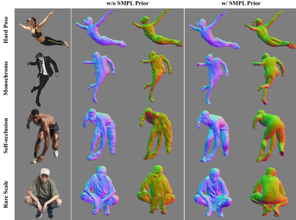
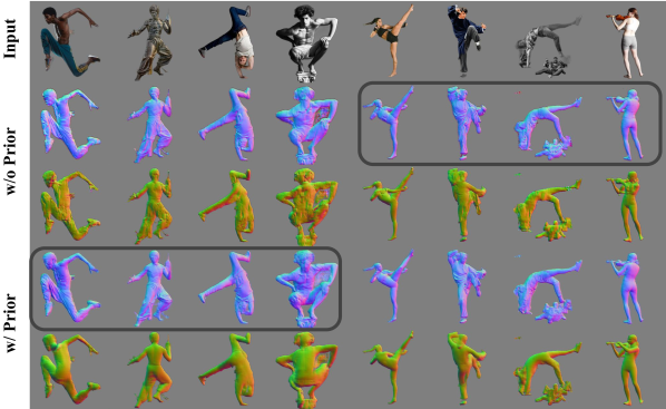
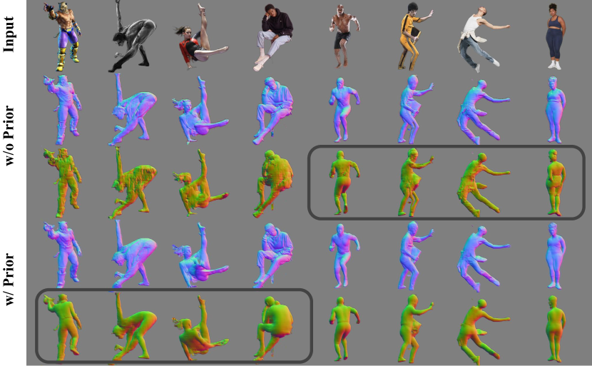
B. Body-guided normal prediction. We evaluate the conditioning on SMPL-X-body normal maps, $\mathcal{N}^{\text{b}}$, for guiding inference of clothed-body normal maps, $\widehat{\mathcal{N}}^{\text{c}}$ (Sec. 3.1). Table 2-B shows performance with (“ICON”) and without (“$\text{ICON}_{\text{N}^{\dagger}}$”) conditioning. With no conditioning, errors on “CAPE” increase slightly. Qualitatively, guidance by body normals heavily improves the inferred normals, especially for occluded body regions; see Fig. 5. We also ablate the effect of the body-normal feature (Sec. 3.2), $\mathcal{F}_{\text{n}}^{\text{b}}$, by removing it; this worsens results, see “ICON w/o $\mathcal{F}_{\text{n}}^{\text{b}}$” in Tab. 2-B.

Figure 5: Normal prediction ($\widehat{\mathcal{N}}^{\text{c}}$) w/ and w/o SMPL prior ($\mathcal{N}^{\text{b}}$).

C. Local-feature based implicit reconstruction. To evaluate the importance of our “local” features (Sec. 3.2), $\mathcal{F}_{\text{P}}$, we replace them with “global” features produced by 2D convolutional filters. These are applied on the image and the clothed-body normal maps (“$\text{ICON}_{\text{enc}(\mathcal{I},\widehat{\mathcal{N}}^{\text{c}})}$” in Tab. 2-C), or only on the normal maps (“$\text{ICON}_{\text{enc}(\widehat{\mathcal{N}}^{\text{c}})}$” in Tab. 2-C). We use a 2-stack hourglass model [25], whose receptive field expands to $46\%$ of the image size. This takes a large image area into account and produces features sensitive to global body pose. This worsens reconstruction performance for out-of-distribution poses, such as in “CAPE-NFP”. For an evaluation of PaMIR’s receptive field size, see Appx

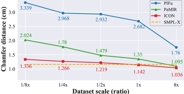
We compare ICON to state-of-the-art (SOTA) models for a varying amount of training data in Fig. 6. The “Dataset scale” axis reports the data size as the ratio w.r.t. the $450$ scans of the original PIFu methods [54, 55]; the left-most side corresponds to $56$ scans and the right-most side corresponds to $3,709$ scans, i.e., all the scans of AGORA [47] and THuman [71]. ICON consistently outperforms all methods. Importantly, ICON achieves SOTA performance even when trained on just a fraction of the data. We attribute this to the local nature of ICON’s point features; this helps ICON generalize well in the pose space and be data efficient.

Figure 6: Reconstruction error w.r.t. training-data size. “Dataset size” is defined as the ratio w.r.t. the $450$ scans used in [54, 55]. The “8x” setting is all $3,709$ scans of AGORA [47] and THuman [71].

D. Robustness to SMPL-X noise. SMPL-X estimated from an image might not be perfectly aligned with body pixels in the image. However, PaMIR and ICON are conditioned on this estimation. Thus, they need to be robust against various noise levels in SMPL-X shape and pose. To evaluate this, we feed $\text{PaMIR}^{*}$ and ICON with ground-truth and perturbed SMPL-X, denoted with (✓) and (✓) in Tab. 2-A,D. ICON conditioned on perturbed (✓) SMPL-X produces larger errors w.r.t. conditioning on ground truth (✓). However, adding the body refinement module (“ICON +BR”) of Sec. 3.1, refines SMPL-X and improves performance. As a result, “ICON +BR” conditioned on noisy SMPL-X (✓) performs comparably to $\text{PaMIR}^{*}$ conditioned on ground-truth SMPL-X (✓); it is slightly worse/better for in-/out-of-distribution poses.

5 Applications

5.1 Reconstruction from in-the-wild images

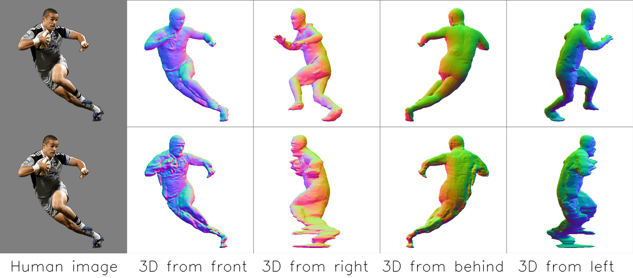
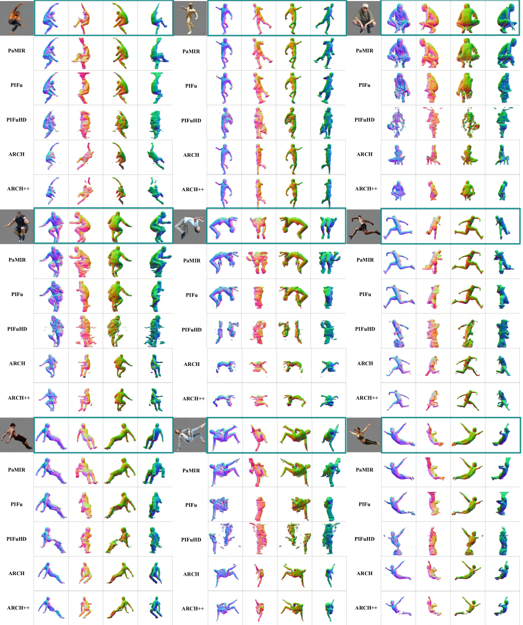
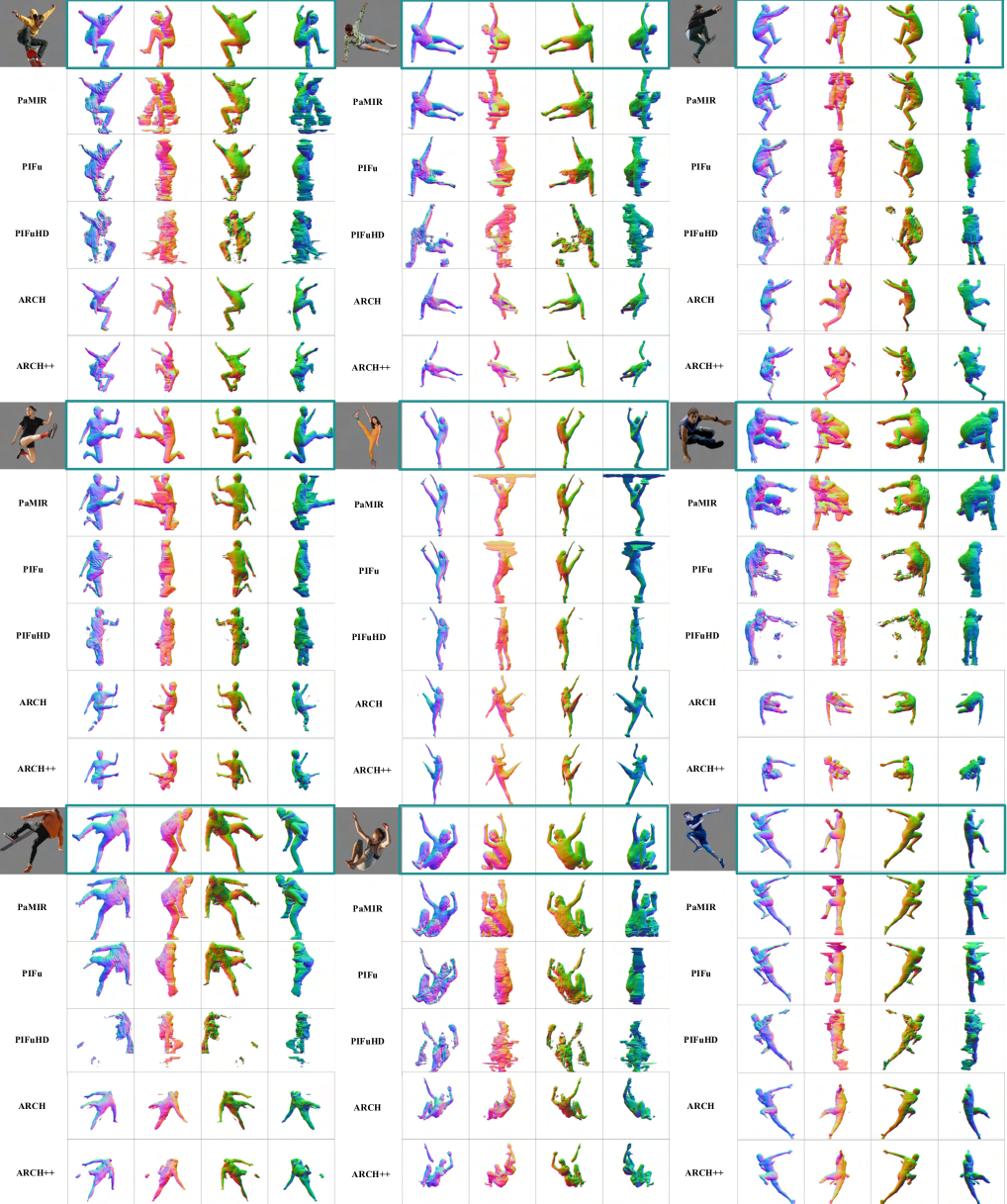
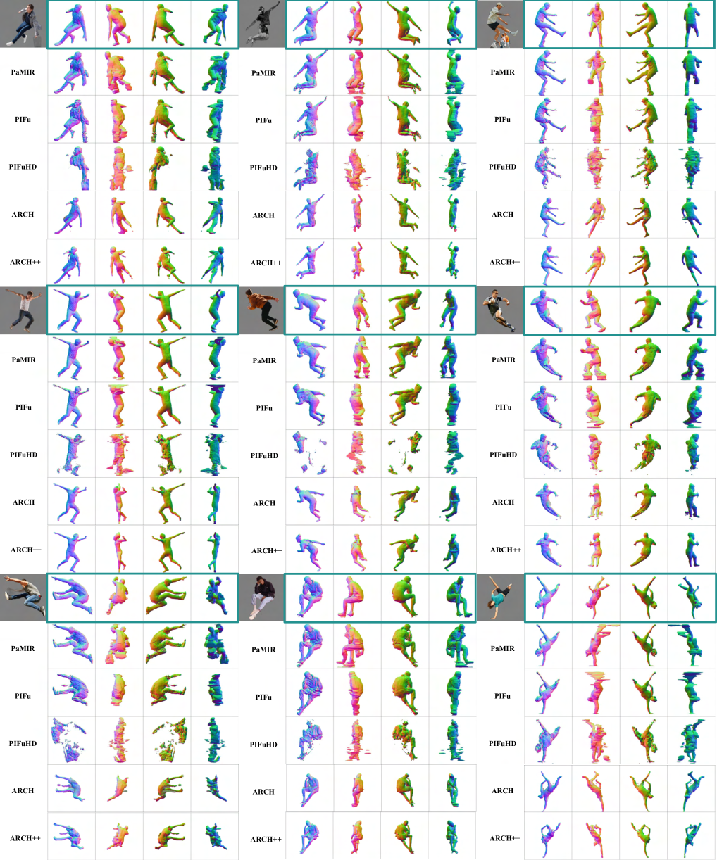
We collect $200$ in-the-wild images from Pinterest that show people performing parkour, sports, street dance, and kung fu. These images are unseen during training. We show qualitative results for ICON in Fig. 7(a) and comparisons to SOTA in Fig. 2; for more results see our video and Appx

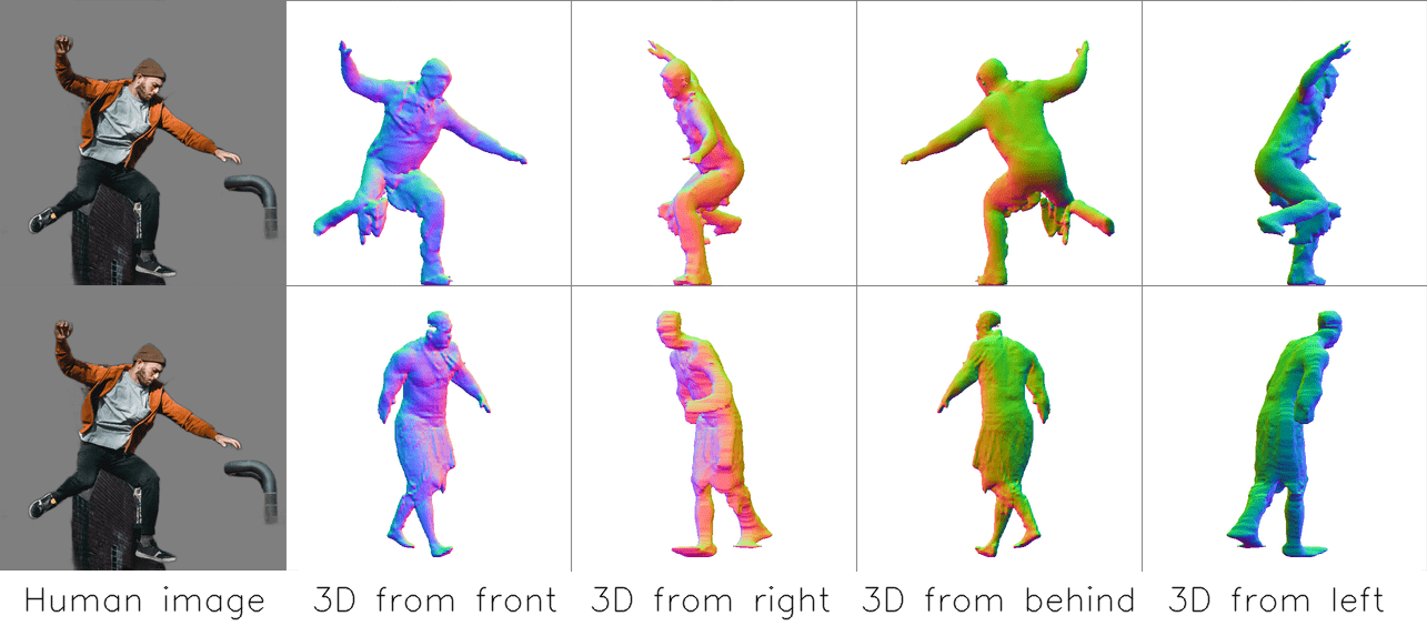
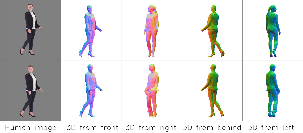
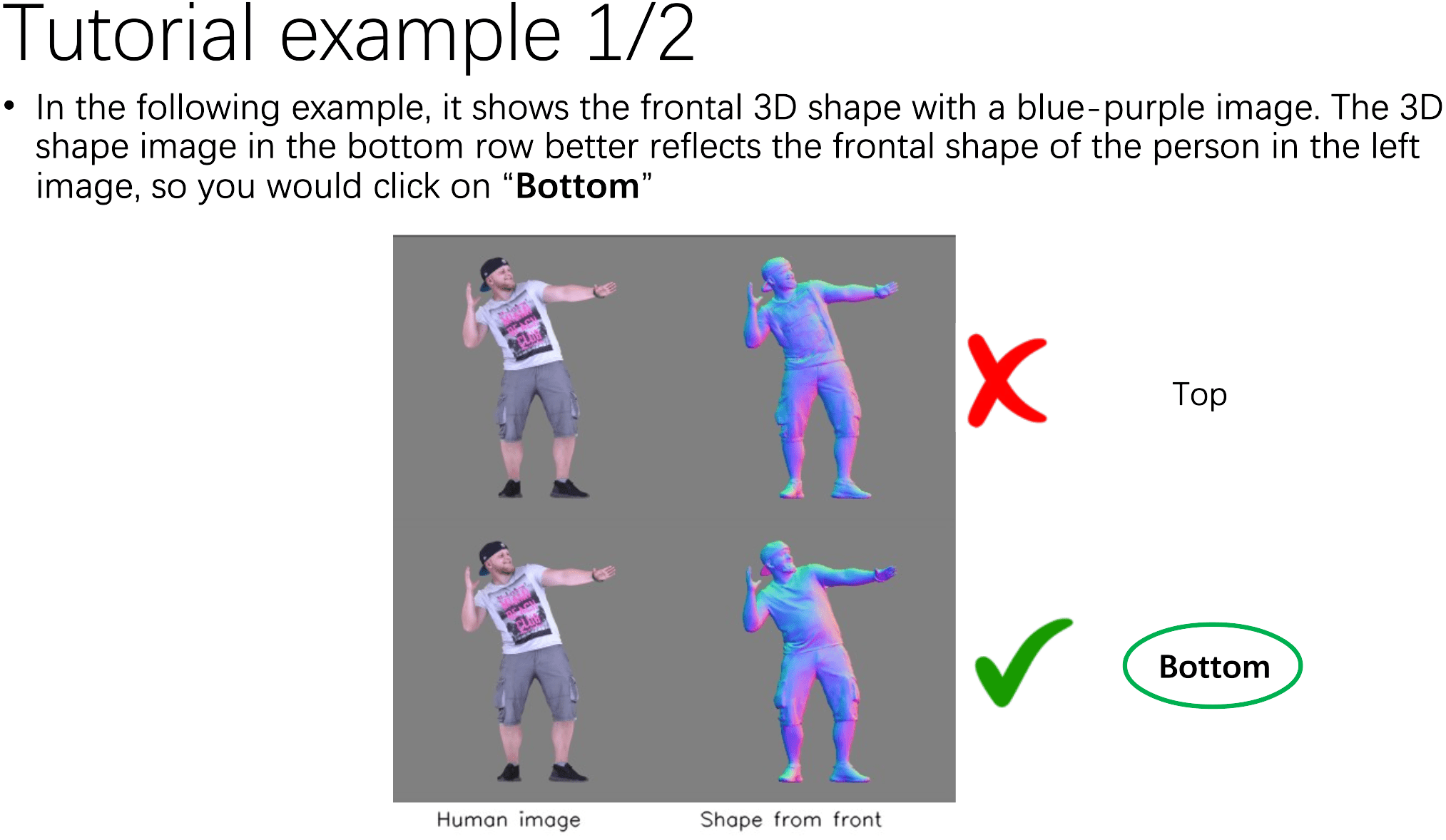
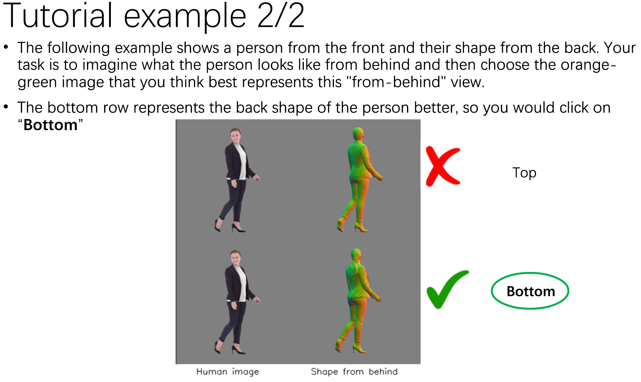
To evaluate the perceived realism of our results, we compare ICON to $\text{PIFu}^{*}$, $\text{PaMIR}^{*}$, and the original PIFuHD [55] in a perceptual study. ICON, $\text{PIFu}^{*}$ and $\text{PaMIR}^{*}$ are trained on all $3,709$ scans of AGORA [47] and THuman [71] (“8x” setting in Fig. 6). For PIFuHD we use its pre-trained model. In the study, participants were shown an image and either a rendered result of ICON or of another method. Participants were asked to choose the result that best represents the shape of the human in the image. We report the percentage of trails in which participants preferred the baseline methods over ICON in Tab. 3; p-values correspond to the null-hypothesis that two methods perform equally well. For details on the study, example stimuli, catch trials, etc. see Appx

5.2 Animatable avatar creation from video

Given a sequence of images with the same subject in various poses, we create an animatable avatar with the help of SCANimate [56]. First, we use ICON to reconstruct a 3D clothed-human mesh per frame. Then, we feed these meshes to SCANimate. ICON’s robustness to diverse poses enables us to learn a clothed avatar with pose-dependent clothing deformation. Unlike raw 3D scans, which are taken with multi-view systems, ICON operates on a single image and its reconstructions are more reliable for observed body regions than for occluded ones. Thus, we reformulate the loss of SCANimate to downweight occluded regions depending on camera viewpoint. Results are shown in ICON: Implicit Clothed humans Obtained from Normals and Fig. 7(b); for animations see the video on our webpage.

Figure 7: Failure cases of ICON for extreme clothing, pose, or camera view. We show the front (blue) and rotated (bronze) views.

	$\text{PIFu}^{*}$	PIFuHD [55]	$\text{PaMIR}^{*}$
Preference	30.9%	22.3%	26.6%
P-value	1.35e-33	1.08e-48	3.60e-54

Table 3: Perceptual study. Numbers denote the chance that participants prefer the reconstruction of a competing method over ICON for in-the-wild images. ICON is judged significantly more realistic.

(a) ICON reconstructions for in-the-wild images with extreme poses (Sec. 5.1).

(b) Avatar creation from images with SCANimate (Sec. 5.2). The input per-frame meshes are reconstructed with ICON.

Figure 8: ICON results for two applications (Sec. 5). We show two views for each mesh, i.e., a front (blue) and a rotated (bronze) view.

6 Conclusion

We have presented ICON, which robustly recovers a 3D clothed person from a single image with accuracy and realism that exceeds prior art. There are two keys: (1) Regularizing the solution with a 3D body model while optimizing that body model iteratively. (2) Using local features to eliminate spurious correlations with global pose. Thorough ablation studies validate these choices. The quality of results is sufficient to build a 3D avatar from monocular image sequences.

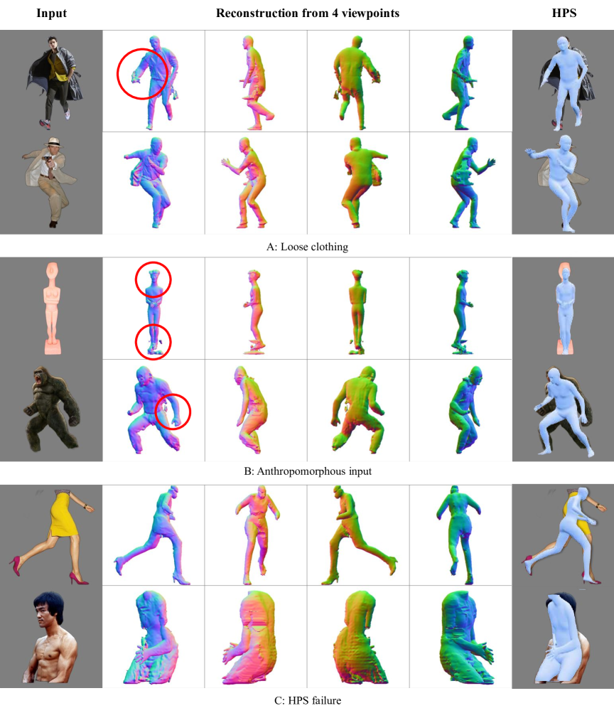
Limitations and future work. Due to the strong body prior exploited by ICON, loose clothing that is far from the body may be difficult to reconstruct; see Fig. 7. Although ICON is robust to small errors of body fits, significant failure of body fits leads to reconstruction failure. Because it is trained on orthographic views, ICON has trouble with strong perspective effects, producing asymmetric limbs or anatomically improbable shapes. A key future application is to use images alone to create a dataset of clothed avatars. Such a dataset could advance research in human shape generation [15], be valuable to fashion industry, and facilitate graphics applications.

Possible negative impact. While the quality of virtual humans created from images is not at the level of facial “deep fakes”, as this technology matures, it will open up the possibility for full-body deep fakes, with all the attendant risks. These risks must also be balanced by the positive use cases in entertainment, tele-presence, and future metaverse applications. Clearly regulation will be needed to establish legal boundaries for its use. In lieu of societal guidelines today, we have made our code available with an appropriate license.

Disclosure. https://files.is.tue.mpg.de/black/CoI_CVPR_2022.txt

Acknowledgments. We thank Yao Feng, Soubhik Sanyal, Hongwei Yi, Qianli Ma, Chun-Hao Paul Huang, Weiyang Liu, and Xu Chen for their feedback and discussions, Tsvetelina Alexiadis for her help with perceptual study, Taylor McConnell assistance, Benjamin Pellkofer for webpage, and Yuanlu Xu’s help in comparing with ARCH and ARCH++. This project has received funding from the European Union’s Horizon $2020$ research and innovation programme under the Marie Skłodowska-Curie grant agreement No.$860768$ (CLIPE project).

We provide more details for the method and experiments, as well as more quantitative and qualitative results, as an extension of Sec. 3, Sec. 4 and Sec. 5 of the main paper.

Appendix A Method & Experiment Details

A.1 Dataset (Sec. 4.2)

Dataset size. We evaluate the performance of ICON and SOTA methods for a varying training-dataset size (Figs. 6 and 9). For this, we first combine AGORA  [47] ($3,109$ scans) and THuman [71] ($600$ scans) to get $3,709$ scans in total. This new dataset is $8$x times larger than the $450$ Renderpeople (“$450$-Rp”) scans used in [54, 55]. Then, we sample this “$8$x dataset” to create smaller variations, for $1/8$x, $1/4$x, $1/2$x, $1$x, and $8$x the size of “$450$-Rp”.

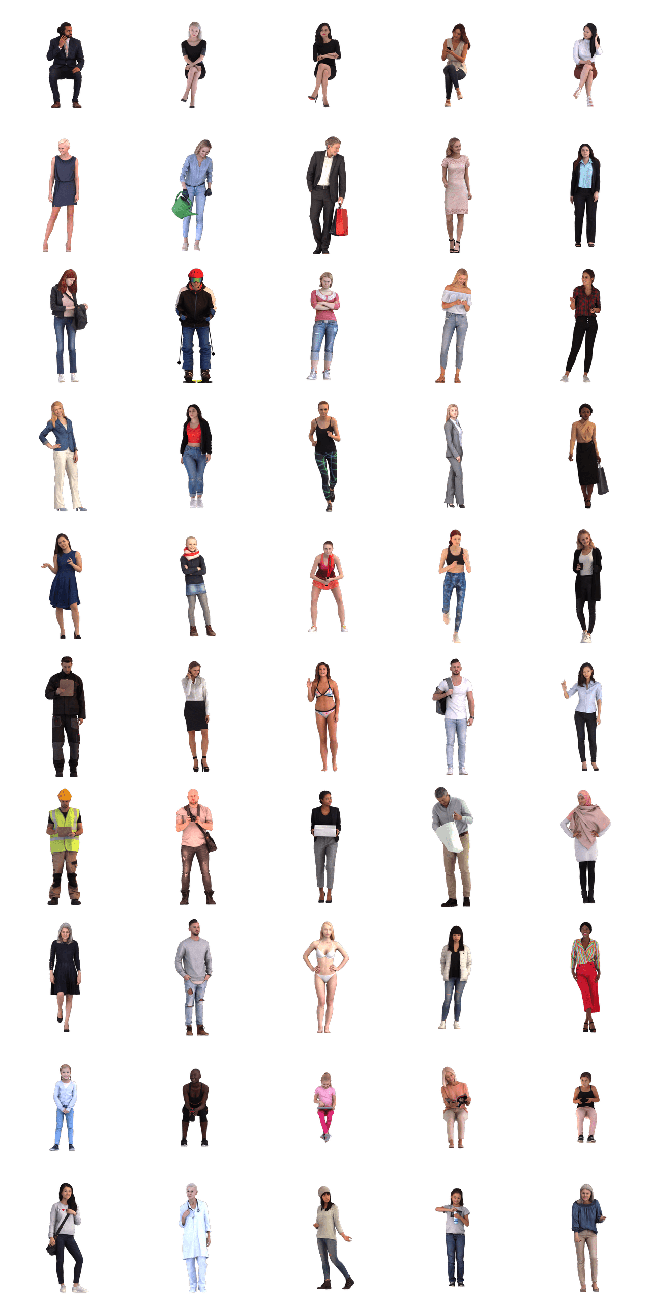
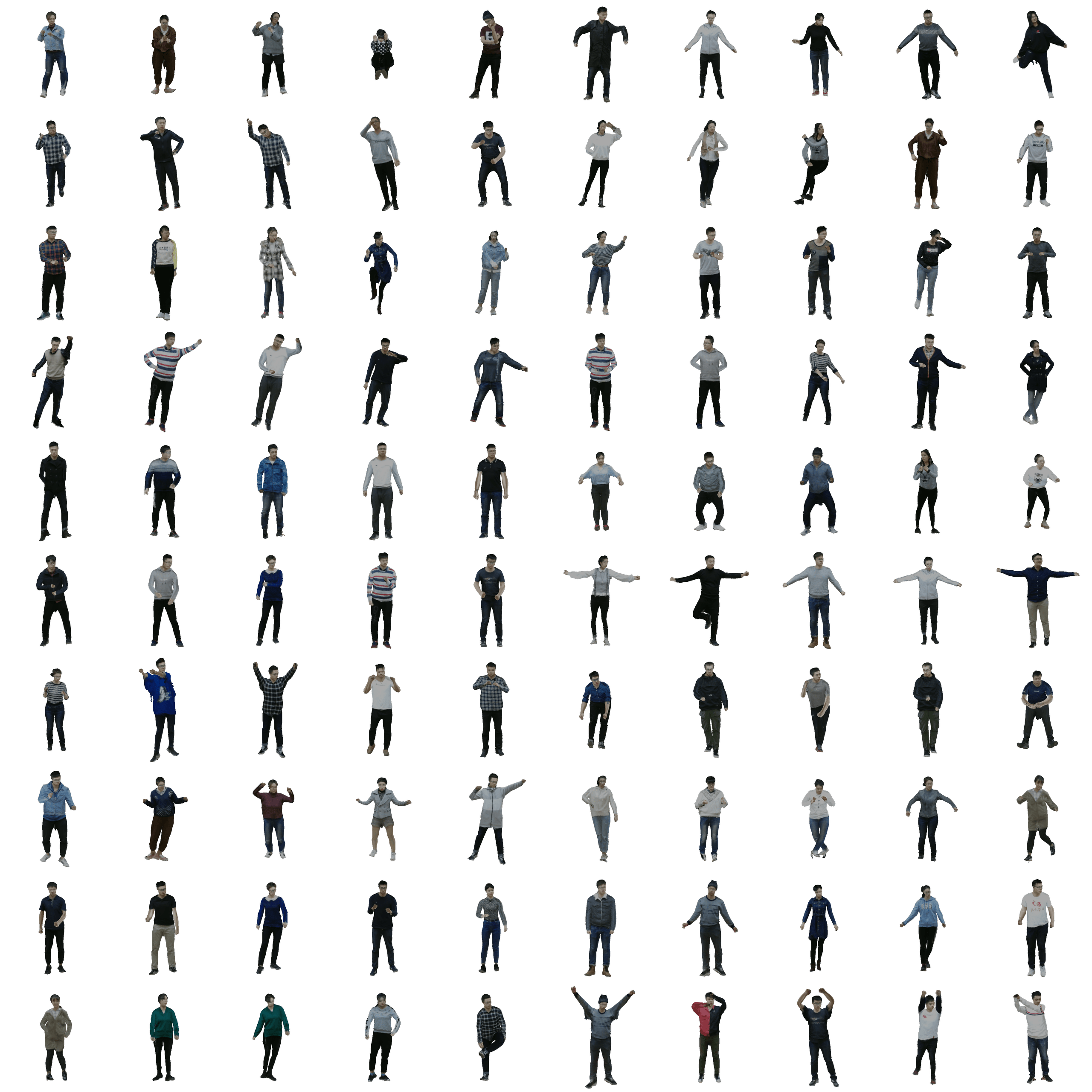
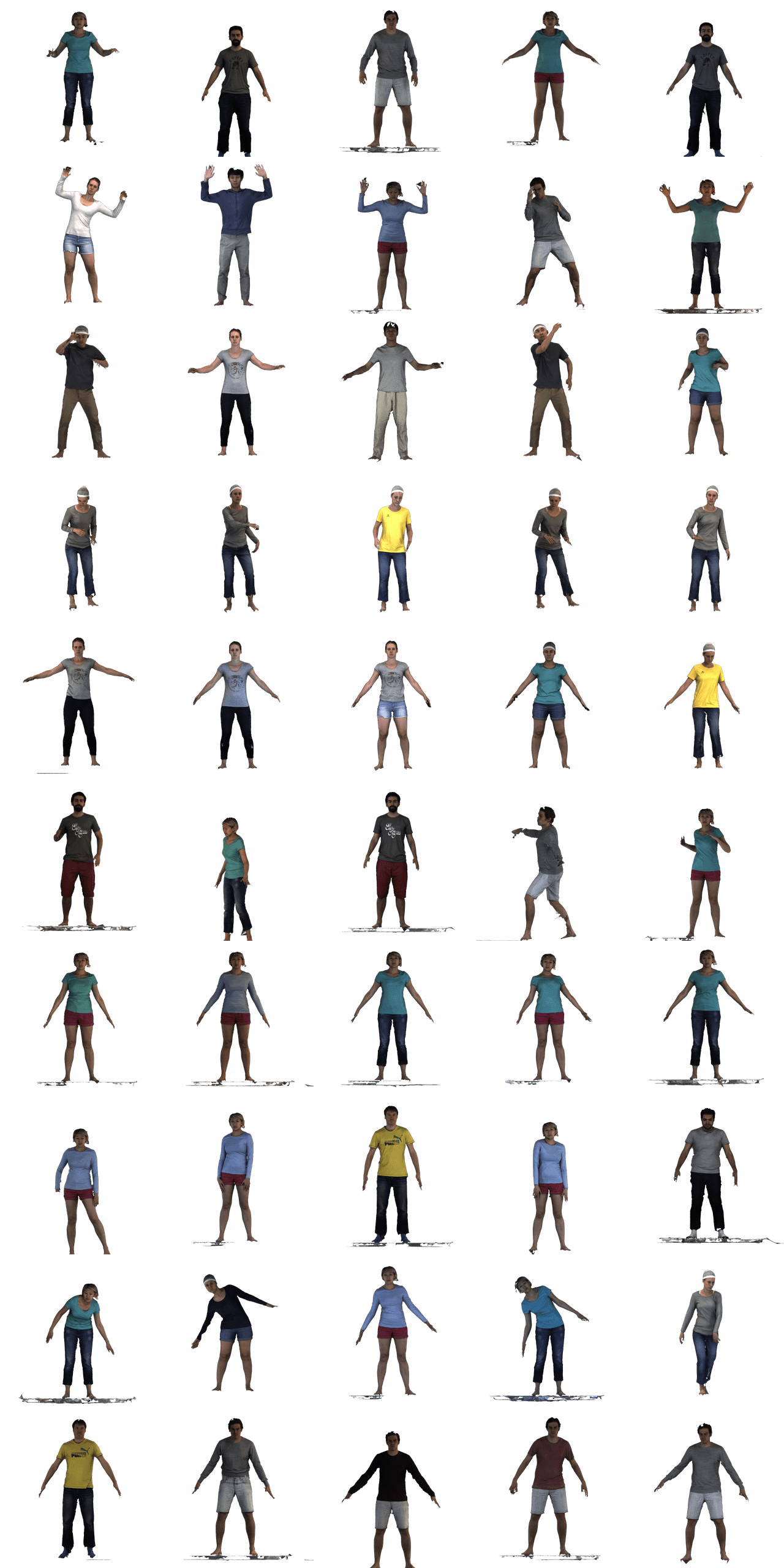
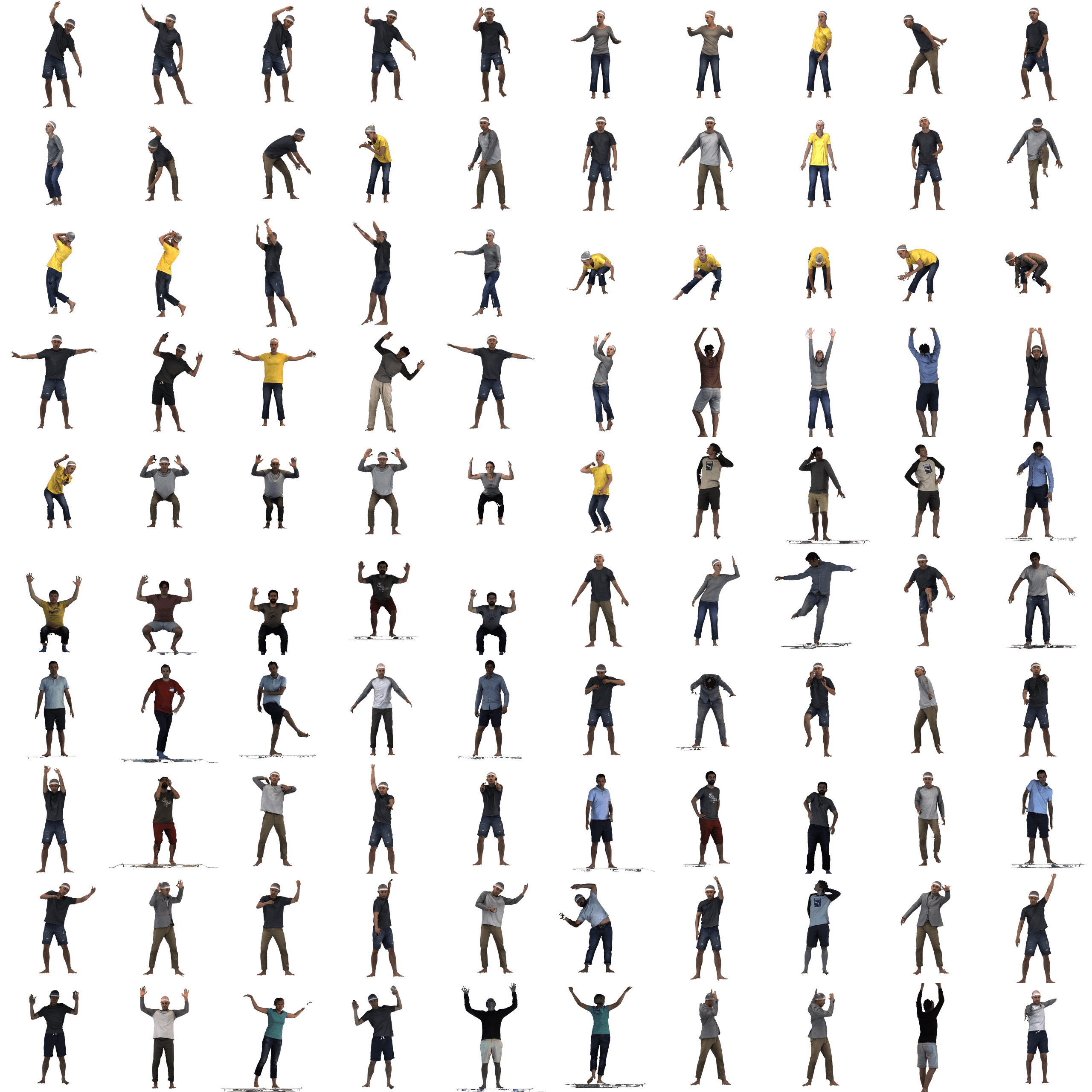
Dataset splits. For the “$8$x dataset”, we split the $3,109$ AGORA scans into a new training set ($3,034$ scans), validation set ($25$ scans) and test set ($50$ scans). Among these, $1,847$ come from Renderpeople [3] (see Fig. 9(a)), $622$ from AXYZ [8], $242$ from Humanalloy [2], $398$ from 3DPeople [1], and we sample only $600$ scans from THuman (see Fig. 9(b)), due to its high pose repeatability and limited identity variants (see Tab. 1), with the “select-cluster” scheme described below. These scans, as well as their SMPL-X fits, are rendered after every $10$ degrees rotation around the yaw axis, to totally generate $(3109\text{~{}\mbox{AGORA}}+600\text{~{}\mbox{THuman}}+150\text{~{}\mbox{CAPE}})\times 36=138,924$ samples.

Dataset distribution via “select-cluster” scheme. To create a training set with a rich pose distribution, we need to select scans from various datasets with poses different from AGORA. Following SMPLify [13], we first fit a Gaussian Mixture Model (GMM) with $8$ components to all AGORA poses, and select 2K THuman scans with low likelihood. Then, we apply M-Medoids ($\text{n\_cluster}=50$) on these selections for clustering, and randomly pick $12$ scans per cluster, collecting $50\times 12=600$ THuman scans in total; see Fig. 9(b). This is also used to split CAPE into “CAPE-FP” (Fig. 9(c)) and “CAPE-NFP” (Fig. 9(d)), corresponding to scans with poses similar (in-distribution poses) and dissimilar (out-of-distribution poses) to AGORA ones, respectively.

Perturbed SMPL. To perturb SMPL’s pose and shape parameters, random noise is added to $\theta\text{ and }\beta$ by:

$$\begin{gathered}\theta\mathrel{+}=s_{\theta}*\mu\text{,}\\ \beta\mathrel{+}=s_{\beta}*\mu\text{,}\\ \end{gathered}$$ (8)

where $\mu\in[-1,1]$, $s_{\theta}=0.15$ and $s_{\beta}=0.5$. These are set empirically to mimic the misalignment error typically caused by off-the-shell HPS during testing.

Discussion on simulated data. The wide and loose clothing in CLOTH3D++ [9, 43] demonstrates strong dynamics, which would complement commonly used datasets of commercial scans. Yet, the domain gap between CLOTH3D++ and real images is still large. Moreover, it is unclear how to train an implicit function from multi-layer non-watertight meshes. Consequently, we leave it for future research.

A.2 Refining SMPL (Sec. 3.1)

Figure 9: SMPL refinement error (y-axis) with different losses (see colors) and noise levels, $s_{\theta}$, of pose parameters (x-axis).

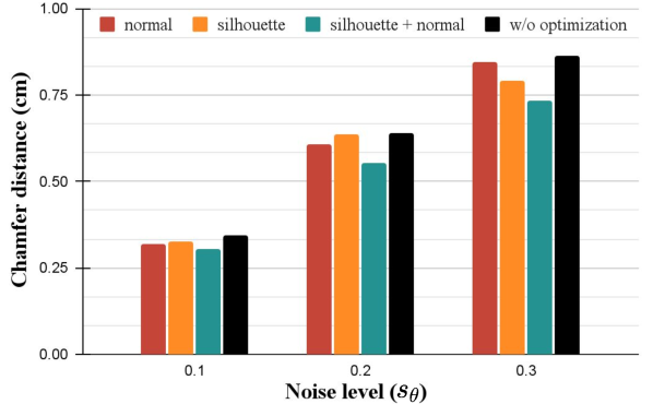
To statistically analyze the necessity of $\mathcal{L}_{\text{N\_diff}}$ and $\mathcal{L}_{\text{S\_diff}}$ in Eq. 4, we do a sanity check on AGORA’s validation set. Initialized with different pose noise, $s_{\theta}$ (Eq. 8), we optimize the $\{\theta,\beta,t\}$ parameters of the perturbed SMPL by minimizing the difference between rendered SMPL-body normal maps and ground-truth clothed-body normal maps for 2K iterations. As Fig. 9 shows, $\mathcal{L}_{\text{N\_diff}}+\mathcal{L}_{\text{S\_diff}}$ always leads to the smallest error under any noise level, measured by the Chamfer distance between the optimized perturbed SMPL mesh and the ground-truth SMPL mesh.

	Methods	SMPL-X	AGORA-50			CAPE-FP			CAPE-NFP			CAPE
		condition.	Chamfer $\downarrow$	P2S $\downarrow$	Normal $\downarrow$	Chamfer $\downarrow$	P2S $\downarrow$	Normal $\downarrow$	Chamfer $\downarrow$	P2S $\downarrow$	Normal $\downarrow$	Chamfer $\downarrow$	P2S $\downarrow$	Normal $\downarrow$
	ICON	✓	1.583	1.987	0.079	1.364	1.403	0.080	1.444	1.453	0.083	1.417	1.436	0.082
D	SMPL-X perturbed	✓	1.984	2.471	0.098	1.488	1.531	0.095	1.493	1.534	0.098	1.491	1.533	0.097
	$\text{ICON}_{\text{enc(I,N)}}$	✓	1.569	1.784	0.073	1.379	1.498	0.070	1.600	1.580	0.078	1.526	1.553	0.075
	$\text{ICON}_{\text{enc(N)}}$	✓	1.564	1.854	0.074	1.368	1.484	0.071	1.526	1.524	0.078	1.473	1.511	0.076
	$\text{ICON}_{\text{N}^{\dagger}}$	✓	1.575	2.016	0.077	1.376	1.496	0.076	1.458	1.569	0.080	1.431	1.545	0.079

Table 4: Quantitative errors (cm) for several ICON variants conditioned on perturbed SMPL-X fits ($s_{\theta}=0.15,s_{\beta}=0.5$).

A.3 Perceptual study (Tab. 3)

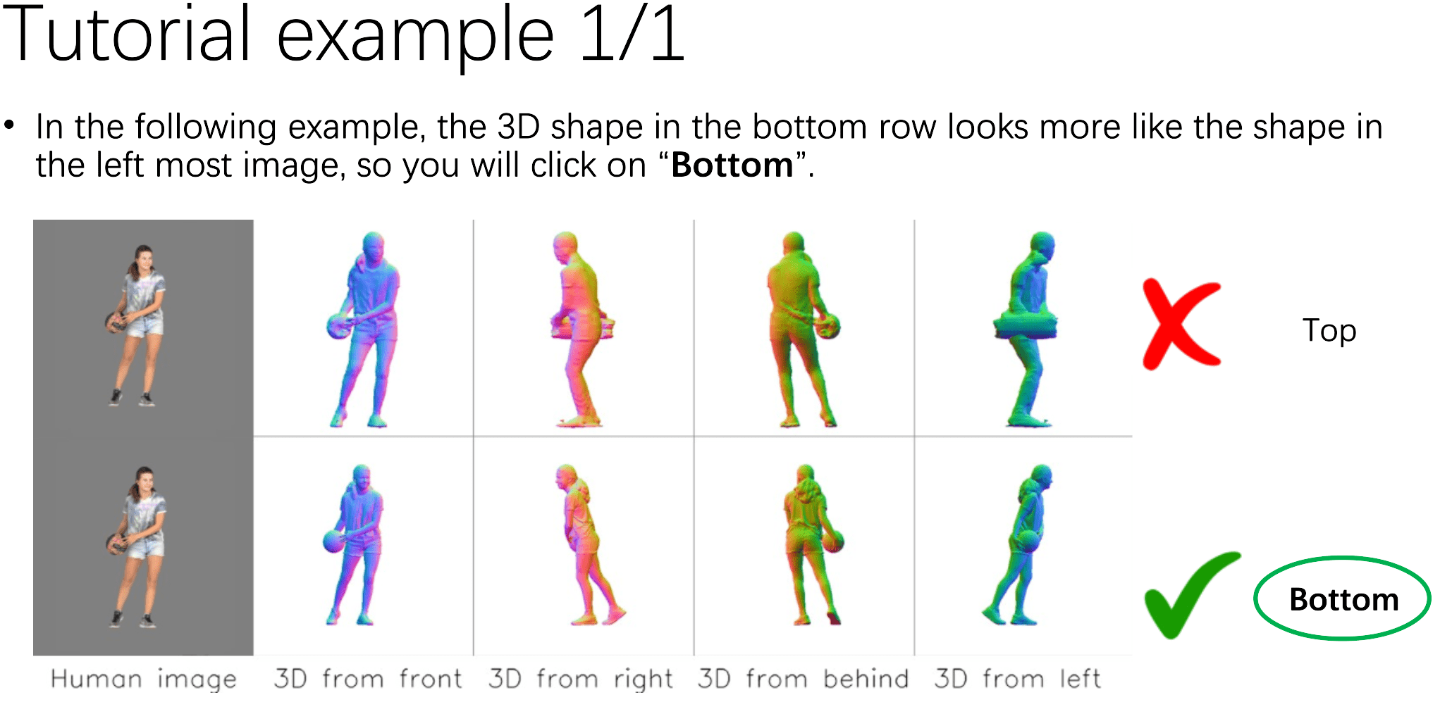
Reconstruction on in-the-wild images. We perform a perceptual study to evaluate the perceived realism of the reconstructed clothed 3D humans from in-the-wild images. ICON is compared against $3$ methods, PIFu [54], PIFuHD [55], and PaMIR [70]. We create a benchmark of $200$ unseen images downloaded from the internet, and apply all the methods on this test set. All the reconstruction results are evaluated on Amazon Mechanical Turk (AMT), where each participant is shown pairs of reconstructions from ICON and one of the baselines, see Fig. 11. Each reconstruction result is rendered in four views: front, right, back and left. Participants are asked to choose the reconstructed 3D shape that better represents the human in the given color image. Each participant is given $100$ samples to evaluate. To teach participants, and to filter out the ones that do not understand the task, we set up $1$ tutorial sample, followed by $10$ warm-up samples, and then the evaluation samples along with catch trial samples inserted every $10$ evaluation samples. Each catch trial sample shows a color image along with either (1) the reconstruction of a baseline method for this image and the ground-truth scan that was rendered to create this image, or (2) the reconstruction of a baseline method for this image and the reconstruction for a different image (false positive), see Fig. 10(c). Only participants that pass $70\%$ out of $10$ catch trials are considered. This leads to $28$ valid participants out of $36$ ones. Results are reported in Tab. 3.

Normal map prediction. To evaluate the effect of the body prior for normal map prediction on in-the-wild images, we conduct a perceptual study against prediction without the body prior. We use AMT, and show participants a color image along with a pair of predicted normal maps from two methods. Participants are asked to pick the normal map that better represents the human in the image. Front- and back-side normal maps are evaluated separately. See Fig. 12 for some samples. We set up $2$ tutorial samples, 10 warm-up samples, $100$ evaluation samples and $10$ catch trials for each subject. The catch trials lead to $20$ valid subjects out of $24$ participants. We report the statistical results in Tab. 5. A chi-squared test is performed with a null hypothesis that the body prior does not have any influence. We show some results in Fig. 13, where all participants unanimously prefer one method over the other. While results of both methods look generally similar on front-side normal maps, using the body prior usually leads to better back-side normal maps.

	w/ SMPL prior	w/o SMPL prior	P-value
Preference (front)	47.3%	52.7%	8.77e-2
Preference (back)	52.9%	47.1%	6.66e-2

Table 5: Perceptual study on normal prediction.

	w/ global	pixel	point	total
	encoder	dims	dims	dims
$\text{PIFu}^{*}$	✓	12	1	13
$\text{PaMIR}^{*}$	✓	6	7	13
$\text{ICON}_{\text{enc(I,N)}}$	✓	6	7	13
$\text{ICON}_{\text{enc(N)}}$	✓	6	7	13
ICON	✗	0	7	7

Table 6: Feature dimensions for various approaches. “pixel dims” and “point dims” denote the feature dimensions encoded from pixels (image/normal maps) and 3D body prior, respectively.

A.4 Implementation details (Sec. 4.1)

Network architecture. Our body-guided normal prediction network uses the same architecture as PIFuHD [55], originally proposed in [28], and consisting of residual blocks with $4$ down-sampling layers. The image encoder for $\text{PIFu}^{*}$, $\text{PaMIR}^{*}$, and $\text{ICON}_{\text{enc}}$ is a stacked hourglass [45] with $2$ stacks, modified according to [25]. Tab. 6 lists feature dimensions for various methods; “total dims” is the neuron number for the first MLP layer (input). The number of neurons in each MLP layer is: $13$ ($7$ for ICON), $512$, $256$, $128$, and $1$, with skip connections at the $3$rd, $4$th, and $5$th layers.

Training details. For training $\mathcal{G}^{\text{N}}$ we do not use THuman due to its low-quality texture (see Tab. 1). On the contrary, $\mathcal{IF}$ is trained on both AGORA and THuman. The front-side and back-side normal prediction networks are trained individually with batch size of $12$ under the objective function defined in Eq. 3, where we set $\lambda_{\text{VGG}}=5.0$. We use the ADAM optimizer with a learning rate of $1.0\times 10^{-4}$ until convergence at $80$ epochs.

Test-time details. During inference, to iteratively refine SMPL and the predicted clothed-body normal maps, we perform $50$ iterations (each iteration takes $\sim 460$ ms on a Quadro RTX $5000$ GPU) and set $\lambda_{\text{N}}=2.0$ in Eq. 4. We conduct an experiment to show the influence of the number of iterations (#iterations) on accuracy, see Tab. 8.

The resolution of the queried occupancy space is $256^{3}$. We use rembg to segment the humans in in-the-wild images, and use Kaolin to compute per-point the signed distance, $\mathcal{F}_{\text{s}}$, and barycentric surface normal, $\mathcal{F}_{\text{n}}^{\text{b}}$.

# iters (460ms/it)	0	10	50
Chamfer $\downarrow$	1.417	1.413	1.339
P2S $\downarrow$	1.436	1.515	1.378
Normal $\downarrow$	0.082	0.077	0.074

Table 7: ICON errors w.r.t. iterations

Receptive field	139	271	403
Chamfer $\downarrow$	1.418	1.478	1.366
P2S $\downarrow$	1.236	1.320	1.214
Normal $\downarrow$	0.083	0.084	0.078

Table 8: PaMIR’s receptive field

Discussion on receptive field size. As Tab. 8 shows, simply reducing the size of receptive field of PaMIR does not lead to better performance. This shows that our informative 3D features as in Eq. 6 and normal maps $\widehat{\mathcal{N}}^{\text{c}}$ also play important roles for robust reconstruction. A more sophisticated design of smaller receptive field may lead to better performance and we would leave it for future research.

Appendix B More Quantitative Results (Sec. 4.3)

Table 4 compares several ICON variants conditioned on perturbed SMPL-X meshes. For the plot of Fig. 6 of the main paper (reconstruction error w.r.t. training-data size), extended quantitative results are shown in Tab. 9.

Training set scale		1/8x	1/4x	1/2x	1x	8x
$\text{PIFu}^{*}$	Chamfer $\downarrow$	3.339	2.968	2.932	2.682	1.760
	P2S $\downarrow$	3.280	2.859	2.812	2.658	1.547
$\text{PaMIR}^{*}$	Chamfer $\downarrow$	2.024	1.780	1.479	1.350	1.095
	P2S $\downarrow$	1.791	1.778	1.662	1.283	1.131
ICON	Chamfer $\downarrow$	1.336	1.266	1.219	1.142	1.036
	P2S $\downarrow$	1.286	1.235	1.184	1.065	1.063

Table 9: Reconstruction error (cm) w.r.t. training-data size. “Training set scale” is defined as the ratio w.r.t. the $450$ scans used in [54, 55]. The “8x” setting is all $3,709$ scans of AGORA [47] and THuman [71]. Results outperform ground-truth SMPL-X, which has 1.158 cm and 1.125 cm for Chamfer and P2S in Tab. 2.

Appendix C More Qualitative Results (Sec. 5)

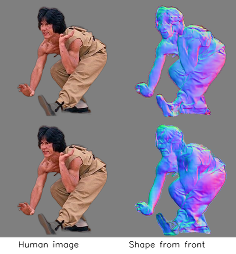
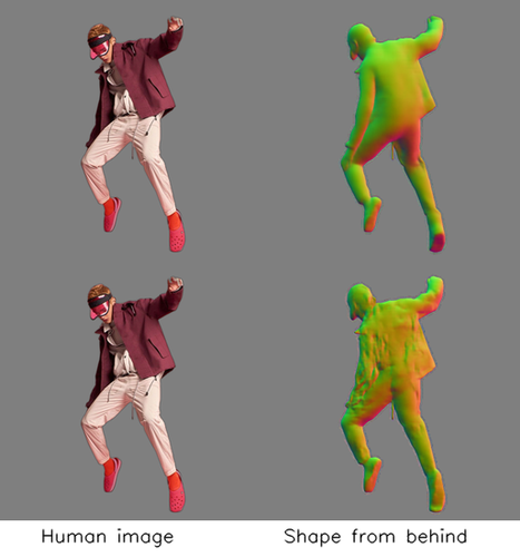
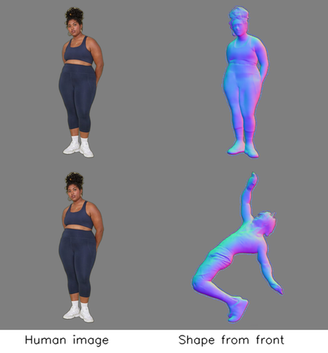
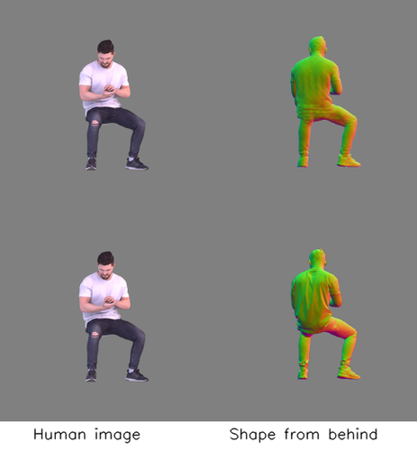
Figures 14, 15 and 16 show reconstructions for in-the-wild images, rendered from four different view points; normals are color coded. Figure 17 shows reconstructions for images with out-of-frame cropping. Figure 18 shows additional representative failures. The video on our website shows animation examples created with ICON and SCANimate.

(a) Renderpeople [3] (450 scans)

(b) THuman [71] (600 scans)

(c) “CAPE-FP” [41] (fashion poses, 50 scans)

(d) “CAPE-NFP” [41] (non fashion poses, 100 scans)

Figure 10: Representative poses for different datasets.

(a) A tutorial sample.

(b) An evaluation sample.

(c) Two samples of catch trials. Left: result from this image (top) vs from another image (bottom). Right: ground-truth (top) vs reconstruction mesh (bottom).

Figure 11: Some samples in the perceptual study to evaluate reconstructions on in-the-wild images.

(a) The two tutorial samples.

(b) Two evaluation samples.

(c) Two catch trial samples.

Figure 12: Some samples in the perceptual study to evaluate the effect of the body prior for normal prediction on in-the-wild images.

(a) Examples of perceptual preference on front normal maps. Unanimously preferred results are in black boxes. The back normal maps are for reference.

(b) Examples of perceptual preference on back normal maps. Unanimously preferred results are in black boxes. The front normal maps are for reference.

Figure 13: Qualitative results to evaluate the effect of body prior for normal prediction on in-the-wild images.

Figure 14: Qualitative comparison of reconstruction for ICON vs SOTA. Four view points are shown per result.

Figure 15: Qualitative comparison of reconstruction for ICON vs SOTA. Four view points are shown per result.

Figure 16: Qualitative comparison of reconstruction for ICON vs SOTA. Four view points are shown per result.

Figure 17: Qualitative comparison (ICON vs SOTA) on images with out-of-frame cropping.

Figure 18: More failure cases of ICON.

References

- [1] 3DPeople. 3dpeople.com, 2018.
- [2] HumanAlloy. humanalloy.com, 2018.
- [3] RenderPeople. renderpeople.com, 2018.
- [4] Thiemo Alldieck, Marcus A. Magnor, Bharat Lal Bhatnagar, Christian Theobalt, and Gerard Pons-Moll. Learning to reconstruct people in clothing from a single RGB camera. In Computer Vision and Pattern Recognition (CVPR), pages 1175–1186, 2019.
- [5] Thiemo Alldieck, Marcus A. Magnor, Weipeng Xu, Christian Theobalt, and Gerard Pons-Moll. Detailed human avatars from monocular video. In International Conference on 3D Vision (3DV), pages 98–109, 2018.
- [6] Thiemo Alldieck, Marcus A. Magnor, Weipeng Xu, Christian Theobalt, and Gerard Pons-Moll. Video based reconstruction of 3D people models. In Computer Vision and Pattern Recognition (CVPR), pages 8387–8397, 2018.
- [7] Thiemo Alldieck, Gerard Pons-Moll, Christian Theobalt, and Marcus A. Magnor. Tex2Shape: Detailed full human body geometry from a single image. In International Conference on Computer Vision (ICCV), pages 2293–2303, 2019.
- [8] AXYZ. secure.axyz-design.com, 2018.
- [9] Hugo Bertiche, Meysam Madadi, and Sergio Escalera. CLOTH3D: Clothed 3D humans. In European Conference on Computer Vision (ECCV), volume 12365, pages 344–359, 2020.
- [10] Bharat Lal Bhatnagar, Cristian Sminchisescu, Christian Theobalt, and Gerard Pons-Moll. Combining implicit function learning and parametric models for 3D human reconstruction. In European Conference on Computer Vision (ECCV), volume 12347, pages 311–329, 2020.
- [11] Bharat Lal Bhatnagar, Cristian Sminchisescu, Christian Theobalt, and Gerard Pons-Moll. LoopReg: Self-supervised learning of implicit surface correspondences, pose and shape for 3D human mesh registration. In Conference on Neural Information Processing Systems (NeurIPS), 2020.
- [12] Bharat Lal Bhatnagar, Garvita Tiwari, Christian Theobalt, and Gerard Pons-Moll. Multi-Garment Net: Learning to dress 3D people from images. In International Conference on Computer Vision (ICCV), pages 5419–5429, 2019.
- [13] Federica Bogo, Angjoo Kanazawa, Christoph Lassner, Peter V. Gehler, Javier Romero, and Michael J. Black. Keep it SMPL: Automatic estimation of 3D human pose and shape from a single image. In European Conference on Computer Vision (ECCV), volume 9909, pages 561–578, 2016.
- [14] Aljaz Bozic, Pablo R. Palafox, Michael Zollhöfer, Justus Thies, Angela Dai, and Matthias Nießner. Neural deformation graphs for globally-consistent non-rigid reconstruction. In Computer Vision and Pattern Recognition (CVPR), pages 1450–1459, 2021.
- [15] Xu Chen, Tianjian Jiang, Jie Song, Jinlong Yang, Michael J. Black, Andreas Geiger, and Otmar Hilliges. gDNA: Towards generative detailed neural avatars. In Computer Vision and Pattern Recognition (CVPR), 2022.
- [16] Xu Chen, Yufeng Zheng, Michael J. Black, Otmar Hilliges, and Andreas Geiger. SNARF: Differentiable forward skinning for animating non-rigid neural implicit shapes. In International Conference on Computer Vision (ICCV), pages 11594–11604, 2021.
- [17] Zhiqin Chen and Hao Zhang. Learning implicit fields for generative shape modeling. In Computer Vision and Pattern Recognition (CVPR), pages 5939–5948, 2019.
- [18] Vasileios Choutas, Lea Müller, Chun-Hao P. Huang, Siyu Tang, Dimitrios Tzionas, and Michael J. Black. Accurate 3D body shape regression via linguistic attributes and anthropometric measurements. In Computer Vision and Pattern Recognition (CVPR), 2022.
- [19] Boyang Deng, JP Lewis, Timothy Jeruzalski, Gerard Pons-Moll, Geoffrey Hinton, Mohammad Norouzi, and Andrea Tagliasacchi. Neural Articulated Shape Approximation. In European Conference on Computer Vision (ECCV), volume 12352, pages 612–628, 2020.
- [20] Zijian Dong, Chen Guo, Jie Song, Xu Chen, Andreas Geiger, and Otmar Hilliges. PINA: Learning a personalized implicit neural avatar from a single RGB-D video sequence. In Computer Vision and Pattern Recognition (CVPR), 2022.
- [21] Yao Feng, Vasileios Choutas, Timo Bolkart, Dimitrios Tzionas, and Michael J. Black. Collaborative regression of expressive bodies using moderation. In International Conference on 3D Vision (3DV), pages 792–804, 2021.
- [22] Tong He, John P. Collomosse, Hailin Jin, and Stefano Soatto. Geo-PIFu: Geometry and pixel aligned implicit functions for single-view human reconstruction. In Conference on Neural Information Processing Systems (NeurIPS), 2020.
- [23] Tong He, Yuanlu Xu, Shunsuke Saito, Stefano Soatto, and Tony Tung. ARCH++: Animation-ready clothed human reconstruction revisited. In International Conference on Computer Vision (ICCV), pages 11046–11056, 2021.
- [24] Zeng Huang, Yuanlu Xu, Christoph Lassner, Hao Li, and Tony Tung. ARCH: Animatable reconstruction of clothed humans. In Computer Vision and Pattern Recognition (CVPR), pages 3090–3099, 2020.
- [25] Aaron S. Jackson, Chris Manafas, and Stefan Roth Georgios Tzimiropoulos. 3D human body reconstruction from a single image via volumetric regression. In European Conference on Computer Vision Workshops (ECCVw), volume 11132, pages 64–77, 2018.
- [26] Yasamin Jafarian and Hyun Soo Park. Learning high fidelity depths of dressed humans by watching social media dance videos. In Computer Vision and Pattern Recognition (CVPR), pages 12753–12762, June 2021.
- [27] Boyi Jiang, Juyong Zhang, Yang Hong, Jinhao Luo, Ligang Liu, and Hujun Bao. BCNet: Learning body and cloth shape from a single image. In European Conference on Computer Vision (ECCV), pages 18–35, 2020.
- [28] Justin Johnson, Alexandre Alahi, and Li Fei-Fei. Perceptual losses for real-time style transfer and super-resolution. In European Conference on Computer Vision (ECCV), volume 9906, pages 694–711, 2016.
- [29] Hanbyul Joo, Tomas Simon, and Yaser Sheikh. Total capture: A 3D deformation model for tracking faces, hands, and bodies. In Computer Vision and Pattern Recognition (CVPR), pages 8320–8329, 2018.
- [30] Angjoo Kanazawa, Michael J. Black, David W. Jacobs, and Jitendra Malik. End-to-end recovery of human shape and pose. In Computer Vision and Pattern Recognition (CVPR), pages 7122–7131, 2018.
- [31] Muhammed Kocabas, Nikos Athanasiou, and Michael J. Black. VIBE: Video inference for human body pose and shape estimation. In Computer Vision and Pattern Recognition (CVPR), pages 5252–5262, 2020.
- [32] Muhammed Kocabas, Chun-Hao P. Huang, Otmar Hilliges, and Michael J. Black. PARE: Part attention regressor for 3D human body estimation. In International Conference on Computer Vision (ICCV), pages 11127–11137, 2021.
- [33] Nikos Kolotouros, Georgios Pavlakos, Michael J. Black, and Kostas Daniilidis. Learning to reconstruct 3D human pose and shape via model-fitting in the loop. In International Conference on Computer Vision (ICCV), pages 2252–2261, 2019.
- [34] Verica Lazova, Eldar Insafutdinov, and Gerard Pons-Moll. 360-Degree textures of people in clothing from a single image. In International Conference on 3D Vision (3DV), pages 643–653, 2019.
- [35] Ruilong Li, Kyle Olszewski, Yuliang Xiu, Shunsuke Saito, Zeng Huang, and Hao Li. Volumetric human teleportation. In ACM SIGGRAPH 2020 Real-Time Live, pages 1–1. 2020.
- [36] Ruilong Li, Yuliang Xiu, Shunsuke Saito, Zeng Huang, Kyle Olszewski, and Hao Li. Monocular real-time volumetric performance capture. In European Conference on Computer Vision (ECCV), volume 12368, pages 49–67, 2020.
- [37] Zhe Li, Tao Yu, Chuanyu Pan, Zerong Zheng, and Yebin Liu. Robust 3D self-portraits in Seconds. In Computer Vision and Pattern Recognition (CVPR), pages 1341–1350, 2020.
- [38] Matthew Loper, Naureen Mahmood, Javier Romero, Gerard Pons-Moll, and Michael J. Black. SMPL: A skinned multi-person linear model. Transactions on Graphics (TOG), 34(6):248:1–248:16, 2015.
- [39] William E. Lorensen and Harvey E. Cline. Marching cubes: A high resolution 3D surface construction algorithm. International Conference on Computer Graphics and Interactive Techniques (SIGGRAPH), 21(4):163–169, 1987.
- [40] Qianli Ma, Shunsuke Saito, Jinlong Yang, Siyu Tang, and Michael J. Black. SCALE: Modeling clothed humans with a surface codec of articulated local elements. In Computer Vision and Pattern Recognition (CVPR), pages 16082–16093, 2021.
- [41] Qianli Ma, Jinlong Yang, Anurag Ranjan, Sergi Pujades, Gerard Pons-Moll, Siyu Tang, and Michael J. Black. Learning to dress 3D people in generative clothing. In Computer Vision and Pattern Recognition (CVPR), pages 6468–6477, 2020.
- [42] Qianli Ma, Jinlong Yang, Siyu Tang, and Michael J. Black. The power of points for modeling humans in clothing. In International Conference on Computer Vision (ICCV), pages 10974–10984, 2021.
- [43] Meysam Madadi, Hugo Bertiche, Wafa Bouzouita, Isabelle Guyon, and Sergio Escalera. Learning cloth dynamics: 3D + texture garment reconstruction benchmark. In Proceedings of the NeurIPS 2020 Competition and Demonstration Track, PMLR, volume 133, pages 57–76, 2021.
- [44] Lars M. Mescheder, Michael Oechsle, Michael Niemeyer, Sebastian Nowozin, and Andreas Geiger. Occupancy networks: Learning 3D reconstruction in function space. In Computer Vision and Pattern Recognition (CVPR), pages 4460–4470, 2019.
- [45] Alejandro Newell, Kaiyu Yang, and Jia Deng. Stacked hourglass networks for human pose estimation. In European Conference on Computer Vision (ECCV), volume 9912, pages 483–499, 2016.
- [46] Jeong Joon Park, Peter Florence, Julian Straub, Richard A. Newcombe, and Steven Lovegrove. DeepSDF: Learning continuous signed distance functions for shape representation. In Computer Vision and Pattern Recognition (CVPR), pages 165–174, 2019.
- [47] Priyanka Patel, Chun-Hao P. Huang, Joachim Tesch, David T. Hoffmann, Shashank Tripathi, and Michael J. Black. AGORA: Avatars in geography optimized for regression analysis. In Computer Vision and Pattern Recognition (CVPR), pages 13468–13478, 2021.
- [48] Georgios Pavlakos, Vasileios Choutas, Nima Ghorbani, Timo Bolkart, Ahmed A. A. Osman, Dimitrios Tzionas, and Michael J. Black. Expressive body capture: 3D hands, face, and body from a single image. In Computer Vision and Pattern Recognition (CVPR), pages 10975–10985, 2019.
- [49] PIFuHD code on GitHub. https://github.com/facebookresearch/pifuhd, 2020.
- [50] Gerard Pons-Moll, Sergi Pujades, Sonny Hu, and Michael J. Black. ClothCap: seamless 4D clothing capture and retargeting. Transactions on Graphics (TOG), 36(4):73:1–73:15, 2017.
- [51] Nikhila Ravi, Jeremy Reizenstein, David Novotny, Taylor Gordon, Wan-Yen Lo, Justin Johnson, and Georgia Gkioxari. Accelerating 3D deep learning with PyTorch3D. arXiv:2007.08501, 2020.
- [52] Rembg: A tool to remove images background. https://github.com/danielgatis/rembg, 2022.
- [53] Javier Romero, Dimitrios Tzionas, and Michael J. Black. Embodied hands: Modeling and capturing hands and bodies together. Transactions on Graphics (TOG), 36(6):245:1–245:17, 2017.
- [54] Shunsuke Saito, Zeng Huang, Ryota Natsume, Shigeo Morishima, Hao Li, and Angjoo Kanazawa. PIFu: Pixel-aligned implicit function for high-resolution clothed human digitization. In International Conference on Computer Vision (ICCV), pages 2304–2314, 2019.
- [55] Shunsuke Saito, Tomas Simon, Jason M. Saragih, and Hanbyul Joo. PIFuHD: Multi-level pixel-aligned implicit function for high-resolution 3D human digitization. In Computer Vision and Pattern Recognition (CVPR), pages 81–90, 2020.
- [56] Shunsuke Saito, Jinlong Yang, Qianli Ma, and Michael J. Black. SCANimate: Weakly supervised learning of skinned clothed avatar networks. In Computer Vision and Pattern Recognition (CVPR), pages 2886–2897, 2021.
- [57] David Smith, Matthew Loper, Xiaochen Hu, Paris Mavroidis, and Javier Romero. FACSIMILE: Fast and accurate scans from an image in less than a second. In International Conference on Computer Vision (ICCV), pages 5330–5339, 2019.
- [58] Yu Sun, Wu Liu, Qian Bao, Yili Fu, Tao Mei, and Michael J. Black. Putting people in their place: Monocular regression of 3D people in depth. In Computer Vision and Pattern Recognition (CVPR), 2022.
- [59] Sicong Tang, Feitong Tan, Kelvin Cheng, Zhaoyang Li, Siyu Zhu, and Ping Tan. A neural network for detailed human depth estimation from a single image. In International Conference on Computer Vision (ICCV), pages 7750–7759, 2019.
- [60] Garvita Tiwari, Nikolaos Sarafianos, Tony Tung, and Gerard Pons-Moll. Neural-GIF: Neural generalized implicit functions for animating people in clothing. In International Conference on Computer Vision (ICCV), pages 11708–11718, 2021.
- [61] Twindom. twindom.com, 2018.
- [62] Shaofei Wang, Marko Mihajlovic, Qianli Ma, Andreas Geiger, and Siyu Tang. MetaAvatar: Learning animatable clothed human models from few depth images. In Conference on Neural Information Processing Systems (NeurIPS), 2021.
- [63] Donglai Xiang, Fabian Prada, Chenglei Wu, and Jessica K. Hodgins. MonoClothCap: Towards temporally coherent clothing capture from monocular RGB video. In International Conference on 3D Vision (3DV), pages 322–332, 2020.
- [64] Hongyi Xu, Eduard Gabriel Bazavan, Andrei Zanfir, William T. Freeman, Rahul Sukthankar, and Cristian Sminchisescu. GHUM & GHUML: Generative 3D human shape and articulated pose models. In Computer Vision and Pattern Recognition (CVPR), pages 6183–6192, 2020.
- [65] Ze Yang, Shenlong Wang, Sivabalan Manivasagam, Zeng Huang, Wei-Chiu Ma, Xinchen Yan, Ersin Yumer, and Raquel Urtasun. S3: Neural shape, skeleton, and skinning fields for 3D human modeling. In Computer Vision and Pattern Recognition (CVPR), pages 13284–13293, 2021.
- [66] Hongwei Yi, Chun-Hao P. Huang, Dimitrios Tzionas, Muhammed Kocabas, Mohamed Hassan, Siyu Tang, Justus Thies, and Michael J. Black. Human-aware object placement for visual environment reconstruction. In Computer Vision and Pattern Recognition (CVPR), 2022.
- [67] Chao Zhang, Sergi Pujades, Michael J. Black, and Gerard Pons-Moll. Detailed, accurate, human shape estimation from clothed 3D scan sequences. In Computer Vision and Pattern Recognition (CVPR), pages 5484–5493, 2017.
- [68] Hongwen Zhang, Yating Tian, Xinchi Zhou, Wanli Ouyang, Yebin Liu, Limin Wang, and Zhenan Sun. Pymaf: 3d human pose and shape regression with pyramidal mesh alignment feedback loop. In International Conference on Computer Vision (ICCV), pages 11446–11456, 2021.
- [69] Yang Zheng, Ruizhi Shao, Yuxiang Zhang, Tao Yu, Zerong Zheng, Qionghai Dai, and Yebin Liu. DeepMultiCap: Performance capture of multiple characters using sparse multiview cameras. In International Conference on Computer Vision (ICCV), pages 6239–6249, 2021.
- [70] Zerong Zheng, Tao Yu, Yebin Liu, and Qionghai Dai. PaMIR: Parametric model-conditioned implicit representation for image-based human reconstruction. Transactions on Pattern Analysis and Machine Intelligence (TPAMI), 2021.
- [71] Zerong Zheng, Tao Yu, Yixuan Wei, Qionghai Dai, and Yebin Liu. DeepHuman: 3D human reconstruction from a single image. In International Conference on Computer Vision (ICCV), pages 7738–7748, 2019.
- [72] Hao Zhu, Xinxin Zuo, Sen Wang, Xun Cao, and Ruigang Yang. Detailed human shape estimation from a single image by hierarchical mesh deformation. In Computer Vision and Pattern Recognition (CVPR), pages 4491–4500, 2019.