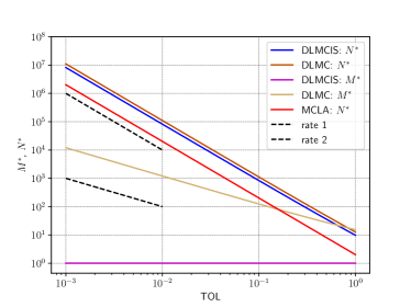
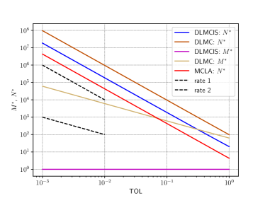
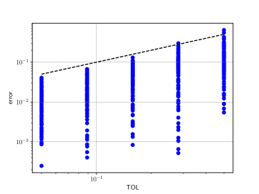
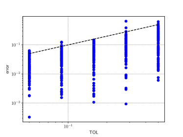
Small-noise approximation for Bayesian optimal experimental design with nuisance uncertainty

Arved Bartuska1, Luis Espath2 & Raúl Tempone1,3,4 1Department of Mathematics, RWTH Aachen University, Gebäude-1953 1.OG, Pontdriesch 14-16, 161, 52062 Aachen, Germany. 2School of Mathematical Sciences, University of Nottingham, Nottingham, NG7 2RD, United Kingdom. 3King Abdullah University of Science & Technology (KAUST), Computer, Electrical and Mathematical Sciences & Engineering Division (CEMSE), Thuwal 23955-6900, Saudi Arabia. 4Alexander von Humboldt Professor in Mathematics for Uncertainty Quantification, RWTH Aachen University, Germany. bartuska@uq.rwth-aachen.de
Abstract.

Calculating the expected information gain in optimal Bayesian experimental design typically relies on nested Monte Carlo sampling. When the model also contains nuisance parameters, which are parameters that contribute to the overall uncertainty of the system but are of no interest in the Bayesian design framework, this introduces a second inner loop. We propose and derive a small-noise approximation for this additional inner loop. The computational cost of our method can be further reduced by applying a Laplace approximation to the remaining inner loop. Thus, we present two methods, the small-noise double-loop Monte Carlo and small-noise Monte Carlo Laplace methods. Moreover, we demonstrate that the total complexity of these two approaches remains comparable to the case without nuisance uncertainty. To assess the efficiency of these methods, we present three examples, and the last example includes the partial differential equation for the electrical impedance tomography experiment for composite laminate materials.
AMS subject classifications: \cdot 65K05 \cdot 65C05 \cdot

1. Introduction

When conducting scientific experiments, information from data is used to learn about the parameters of an underlying model [16]. The relationship between data and parameters depends on the experiment design, which can be regarded as a hyperparameter. Data acquisition is often the most expensive part of an experiment; thus, this design parameter can be optimized beforehand to reduce the number of data points required to achieve a certain error tolerance in the parameters. The amount of information obtained from an experiment can be expressed as the expected Kullback–Leibler divergence [17, 8], also known as the expected information gain (EIG) [20].

Computing this quantity requires evaluating two nested integrals, which are typically not given in closed form. As the straightforward approximation of these integrals using the Monte Carlo method [1] is often prohibitively expensive, several more advanced estimators based on the Laplace approximation [18, 21, 22, 23] have been proposed [2, 3, 4, 5]. These estimators either approximate the inner integral using a second-order Taylor expansion around the mode of the posterior probability density function (pdf) directly or use this approximation for importance sampling to reduce the number of samples required for the inner Monte Carlo estimation. The first approach reduces the order of the average work required but introduces a bias that depends on the number of repetitive experiments, while the second approach has a controllable bias but only reduces constant terms in the asymptotic work requirement. For more details on the Laplace approximation, see [12, 13], where a bound on the approximation error in terms of the Hellinger distance is derived. The approximation error of Laplace-based importance sampling is detailed in [12]. These are asymptotic results for the small noise or large data limit. We only consider a fixed noise level and fixed amount of data. Recently, [29] derived pre-asymptotic error estimates for the Laplace approximation and investigate the effects of the nonlinearity of the forward problem on the non-Gaussianity of the likelihood. Furthermore, [30] provide non-asymptotic guarantees for the Laplace approximation in total variation distance and also consider the case where the maximum aposteriori estimate and Hessian of the log-likelihood are not available directly, but have to be approximated. The concentration of the posterior pdf for time series data and the resulting increased accuracy of the Laplace approximation is discussed in [27]. If the prior pdf has compact support, e.g., a uniform distribution, the posterior distribution exists on the same bounded domain. The Gaussian distribution resulting from the Laplace approximation, however, is unbounded and thus introduces an additional error. In [28], a truncated version of the Laplace approximation is introduced alongside a rejection sampling algorithm to efficiently estimate the expected information gain under this setting.

If the model also contains unknown parameters that are not of immediate interest, we refer to them as nuisance parameters, and the usual approach is to marginalize them [5, 11, 14, 15], leading to a second inner integral and increasing the computational burden. Such a scenario may arise if some of the model’s parameters are not well-calibrated. We will show this for a practical example where the electric conductivity of a material is only given by a concentrated log-normal distribution rather than an exact value. Assuming that the effect of the nuisance parameters is small, we propose using a small-noise approximation combined with the Laplace approximation. The small-noise approximation uses a first-order Taylor approximation of the residual term and a first-order approximation of the resulting likelihood. This method works if the nuisance covariance is sufficiently small compared to the covariance of the error to ensure positive definiteness of the resulting covariance matrix. A slightly different approach was used in [10], where the error covariance was considered an unknown parameter, also requiring marginalization. Another approach is followed in [26], where the authors propose to estimate hyperparameters beforehand and then consider them to be fixed to avoid high-dimensional quadrature for the marginalization.

Our approach differs from that in [5] in the estimators proposed to approximate the EIG functional. Both [5] and our work start out with the same nuisance parameter model, requiring double-loop Monte Carlo approximation with two inner loops. Our contribution lies in proposing a novel small-noise approximation, thus avoiding this additional inner loop at the cost of a bound on the maximum allowed nuisance uncertainty. This bound is consistent with our differing understanding of the interpretation of nuisance parameters. A comparison of the computational work is provided by Remark 1, where we show the optimal number of required samples for two inner loops. We use the small-noise approximation to handle the nuisance uncertainty in a novel manner, which allows us to construct two estimators: one based on the Laplace approximation for the inner integral and one using importance sampling based on the Laplace approximation. The first estimator consists of just one loop but introduces a fixed bias, whereas the second estimator consists of one outer and one inner loop and introduces a controllable bias. The work [5] constructs a multiple-importance sampling scheme that reuses previous model evaluations and consists of one outer and two inner loops. There is also a difference in how we justify the need to deal with nuisance parameters in this model. We aim to extend the data model by including nuisance parameters. In contrast, [5] aimed to reduce the parameter space dimension by regarding some existing parameters as nuisance parameters. Following the distinction between aleatoric and epistemic uncertainty in [6], this means that [5] viewed the nuisance parameters as an epistemic uncertainty and assumed that something could in principle be learned about them. Our approach is agnostic as to the type of uncertainty. The nuisance parameters could also be viewed as an aleatoric uncertainty inaccessible to Bayesian updates, as nothing can be learned about them independent of the chosen design, even for an unlimited amount of data. Similar to [5, 25], we consider the distinction between parameters of interest and nuisance parameters to be a modeling choice. As [11] points out, the marginalization of nuisance parameters can also be formulated in terms of a Quantity of Interest (QoI). The application of the Laplace approximation to optimal design problems w.r.t. a QoI was discussed in [9, 24].

In this paper, we introduce the Bayesian setting in Section 2 and develop the small-noise approximation in Section 3. We use the resulting updated likelihood function in Section 4 and formulate the double-loop Monte Carlo (DLMC) estimator along with the optimal number of outer and inner samples and the error-splitting term. We formulate the Monte Carlo Laplace (MCLA) estimator based on the small-noise approximation in Section 5 and the DLMC estimator with importance sampling (DLMCIS) in Section 6 and derive the optimal setting for both estimators. In Section 7, we present three numerical examples, one to showcase the degradation of the small-noise approximation for a large nuisance error, one linear Gaussian example as presented in [5] to determine the effect of nuisance parameters on the optimal design, and one based on the partial differential equation (PDE) for electrical impedance tomography (EIT) to establish the practical use of the proposed method.

2. Bayesian formulation

Our goal is to determine a design that lets us optimally estimate a vector-valued parameter of interest 𝜽𝜽\boldsymbol{\theta} from measured data 𝒚𝒚\boldsymbol{y} given a mathematical model 𝒈𝒈\boldsymbol{g} of an experiment depending on 𝜽𝜽\boldsymbol{\theta}, 𝒚𝒚\boldsymbol{y}, and a design 𝝃𝝃\boldsymbol{\xi}. In the EIT example [19] discussed in Section 7.3, we consider the fiber orientation of laminate materials as our parameter of interest and the locations of measurement electrodes as the design.

We model the data with additive noise ϵbold-italic-ϵ\boldsymbol{\epsilon}, that is,

(1) 𝒚i(𝝃)=𝒈(𝝃,𝜽t,ϕt)+ϵi.subscript𝒚𝑖𝝃𝒈𝝃subscript𝜽𝑡subscriptbold-italic-ϕ𝑡subscriptbold-italic-ϵ𝑖\boldsymbol{y}_{i}(\boldsymbol{\xi})=\boldsymbol{g}(\boldsymbol{\xi},\text{$\boldsymbol{\theta}_{t}$},\text{$\boldsymbol{\phi}_{t}$})+\text{$\boldsymbol{\epsilon}_{i}$}.

If the model also contains additional parameters ϕbold-italic-ϕ\boldsymbol{\phi} that are of no interest in the Bayesian inference formulation, we refer to them as nuisance parameters and marginalize them. This method can be computationally prohibitive; therefore, other methods are addressed to deal with nuisance parameters. In the EIT example, electric conductivities of the materials are considered nuisance parameters. The model contains the following quantities

  • 𝒚iqsubscript𝒚𝑖superscript𝑞\boldsymbol{y}_{i}\in\mathbb{R}^{q} is the vector of measurements, 1iNe1𝑖subscript𝑁𝑒1\leq i\leq N_{e};

  • 𝒀=(𝒚1,,𝒚Ne)q×Ne𝒀subscript𝒚1subscript𝒚subscript𝑁𝑒superscript𝑞subscript𝑁𝑒\boldsymbol{Y}=(\boldsymbol{y}_{1},\ldots,\boldsymbol{y}_{N_{e}})\in\mathbb{R}^{q\times N_{e}} are the measurements for each experiment;

  • 𝒈q𝒈superscript𝑞\boldsymbol{g}\in\mathbb{R}^{q} denotes the model predictions;

  • ϵiqsubscriptbold-italic-ϵ𝑖superscript𝑞\boldsymbol{\epsilon}_{i}\in\mathbb{R}^{q} is the error vector assumed to be Gaussian ϵ𝒩(𝟎,𝚺ϵ)similar-tobold-italic-ϵ𝒩0subscript𝚺bold-italic-ϵ\boldsymbol{\epsilon}\sim\mathcal{N}(\boldsymbol{0},\boldsymbol{\Sigma}_{\boldsymbol{\epsilon}});

  • 𝜽td𝜽subscript𝜽𝑡superscriptsubscript𝑑𝜽\boldsymbol{\theta}_{t}\in\mathbb{R}^{d_{\boldsymbol{\theta}}} represents the true parameter vector;

  • ϕtdϕsubscriptbold-italic-ϕ𝑡superscriptsubscript𝑑bold-italic-ϕ\boldsymbol{\phi}_{t}\in\mathbb{R}^{d_{\boldsymbol{\phi}}} denotes the true vector of the nuisance parameters;

  • 𝝃s𝝃superscript𝑠\boldsymbol{\xi}\in\mathbb{R}^{s} is the vector of design parameters;

  • q𝑞q indicates the number of measurements; and

  • Nesubscript𝑁𝑒N_{e} is the number of observations under consistent experimental setup.

In this context, the Bayes formula reads

π(𝜽|𝒀,𝝃)𝜋conditional𝜽𝒀𝝃\displaystyle\pi(\boldsymbol{\theta}|\boldsymbol{Y},\boldsymbol{\xi}) =π(𝜽)p(𝒀|𝜽,𝝃)p(𝒀|𝝃)absent𝜋𝜽𝑝conditional𝒀𝜽𝝃𝑝conditional𝒀𝝃\displaystyle=\dfrac{\pi(\boldsymbol{\theta})p(\boldsymbol{Y}|\boldsymbol{\theta},\boldsymbol{\xi})}{p(\boldsymbol{Y}|\boldsymbol{\xi})}
(2) =π(𝜽)𝚽p(𝒀|𝜽,ϕ,𝝃)π(ϕ)dϕ𝚯𝚽p(𝒀|𝜽,ϕ,𝝃)π(ϕ)π(𝜽)dϕd𝜽,absent𝜋𝜽subscript𝚽𝑝conditional𝒀𝜽bold-italic-ϕ𝝃𝜋bold-italic-ϕdifferential-dbold-italic-ϕsubscript𝚯subscript𝚽𝑝conditional𝒀𝜽bold-italic-ϕ𝝃𝜋bold-italic-ϕ𝜋𝜽differential-dbold-italic-ϕdifferential-d𝜽\displaystyle=\dfrac{\pi(\boldsymbol{\theta})\int_{\boldsymbol{\Phi}}p(\boldsymbol{Y}|\boldsymbol{\theta},\boldsymbol{\phi},\boldsymbol{\xi})\pi(\boldsymbol{\phi})\,\mathrm{d}{}\boldsymbol{\phi}}{\int_{\boldsymbol{\Theta}}\int_{\boldsymbol{\Phi}}p(\boldsymbol{Y}|\boldsymbol{\theta},\boldsymbol{\phi},\boldsymbol{\xi})\pi(\boldsymbol{\phi})\pi(\boldsymbol{\theta})\,\mathrm{d}{}\boldsymbol{\phi}\,\mathrm{d}{}\boldsymbol{\theta}},

where the likelihood p(𝒀|𝜽,𝝃)𝑝conditional𝒀𝜽𝝃p(\boldsymbol{Y}|\boldsymbol{\theta},\boldsymbol{\xi}) and evidence p(𝒀|𝝃)𝑝conditional𝒀𝝃p(\boldsymbol{Y}|\boldsymbol{\xi}) terms are obtained by marginalization. We distinguish between p()𝑝p(\cdot) for pdfs of the data and π()𝜋\pi(\cdot) for pdfs of model parameters, namely, the prior distribution π(𝜽)𝜋𝜽\pi(\boldsymbol{\theta}) and the posterior distribution π(𝜽|𝒀,𝝃)𝜋conditional𝜽𝒀𝝃\pi(\boldsymbol{\theta}|\boldsymbol{Y},\boldsymbol{\xi}). The former signifies our knowledge before conducting any experiments, while the latter signifies our knowledge once data is obtained. The term π(ϕ)𝜋bold-italic-ϕ\pi(\boldsymbol{\phi}) is a regular probability density and not a prior distribution that is updated.

Bayesian optimal experimental design aims to determine the experimental setup, as described by the design parameter 𝝃𝝃\boldsymbol{\xi}, for the Bayesian inference of 𝜽tsubscript𝜽𝑡\boldsymbol{\theta}_{t}. We consider batch design similar to [10], where different experimental setups can be expressed by the parameter 𝝃𝝃\boldsymbol{\xi}, which may be a boolean-, integer-, real-, or complex-valued scalar or vector variable. This parameter depends on the particular physical experiment. To carry out the design optimization, we need to establish a relation between an experimental setup and the amount of information that it provides. The information gain based on the Shannon entropy [7] for an experimental design 𝝃𝝃\boldsymbol{\xi} is commonly measured by the Kullback–Leibler divergence [17, 8]. The Kullback–Leibler divergence is given by

(3) DKL=𝚯[log(π(𝜽|𝒀))log(π(𝜽))]π(𝜽|𝒀)d𝜽,subscript𝐷KLsubscript𝚯delimited-[]𝜋conditional𝜽𝒀𝜋𝜽𝜋conditional𝜽𝒀differential-d𝜽D_{\mathrm{KL}}=\int_{\boldsymbol{\Theta}}[\log(\pi(\boldsymbol{\theta}|\boldsymbol{Y}))-\log(\pi(\boldsymbol{\theta}))]\pi(\boldsymbol{\theta}|\boldsymbol{Y})\,\mathrm{d}{}\boldsymbol{\theta},

where the design parameter 𝝃𝝃\boldsymbol{\xi} is omitted for conciseness. The setup must be determined before any experiments are conducted; thus, the marginalization over the data 𝒀𝒀\boldsymbol{Y} must be considered, which is referred to as the EIG [20]:

(4) I=𝒴𝚯[log(π(𝜽|𝒀))log(π(𝜽))]π(𝜽|𝒀)d𝜽p(𝒀)d𝒀.𝐼subscript𝒴subscript𝚯delimited-[]𝜋conditional𝜽𝒀𝜋𝜽𝜋conditional𝜽𝒀differential-d𝜽𝑝𝒀differential-d𝒀I=\int_{\mathcal{Y}}\int_{\boldsymbol{\Theta}}[\log(\pi(\boldsymbol{\theta}|\boldsymbol{Y}))-\log(\pi(\boldsymbol{\theta}))]\pi(\boldsymbol{\theta}|\boldsymbol{Y})\,\mathrm{d}{}\boldsymbol{\theta}p(\boldsymbol{Y})\,\mathrm{d}{}\boldsymbol{Y}.

We replace the posterior pdf using the Bayes formula (2) to arrive at:

(5) I=𝚯𝒴[log(p(𝒀|𝜽))log(p(𝒀))]p(𝒀|𝜽)d𝒀π(𝜽)d𝜽.𝐼subscript𝚯subscript𝒴delimited-[]𝑝conditional𝒀𝜽𝑝𝒀𝑝conditional𝒀𝜽differential-d𝒀𝜋𝜽differential-d𝜽I=\int_{\boldsymbol{\Theta}}\int_{\mathcal{Y}}[\log(p(\boldsymbol{Y}|\boldsymbol{\theta}))-\log(p(\boldsymbol{Y}))]p(\boldsymbol{Y}|\boldsymbol{\theta})\,\mathrm{d}{}\boldsymbol{Y}\pi(\boldsymbol{\theta})\,\mathrm{d}{}\boldsymbol{\theta}.

The goal is to learn about the parameter of interest 𝜽𝜽\boldsymbol{\theta} and not the nuisance parameter ϕbold-italic-ϕ\boldsymbol{\phi}.

The likelihood function is given as follows:

(6) p(𝒀|𝜽,ϕ)det(2π𝚺𝜺)Ne2exp(12i=1Ne𝒓i(𝜽,ϕ,ϵi)𝚺𝜺1𝒓i(𝜽,ϕ,ϵi)),𝑝conditional𝒀𝜽bold-italic-ϕsuperscript2𝜋subscript𝚺𝜺subscript𝑁𝑒212superscriptsubscript𝑖1subscript𝑁𝑒subscript𝒓𝑖𝜽bold-italic-ϕsubscriptbold-italic-ϵ𝑖superscriptsubscript𝚺𝜺1subscript𝒓𝑖𝜽bold-italic-ϕsubscriptbold-italic-ϵ𝑖p(\boldsymbol{Y}|\boldsymbol{\theta},\boldsymbol{\phi})\coloneqq\det(2\pi\boldsymbol{\Sigma}_{\boldsymbol{\varepsilon}})^{-\frac{N_{e}}{2}}\exp\left(-\frac{1}{2}\sum_{i=1}^{N_{e}}\boldsymbol{r}_{i}(\boldsymbol{\theta},\boldsymbol{\phi},\boldsymbol{\epsilon}_{i})\cdot\boldsymbol{\Sigma}_{\boldsymbol{\varepsilon}}^{-1}\boldsymbol{r}_{i}(\boldsymbol{\theta},\boldsymbol{\phi},\boldsymbol{\epsilon}_{i})\right),

where

(7) 𝒓i(𝜽,ϕ,ϵi)𝒚i𝒈(𝜽,ϕ)=𝒈(𝜽t,ϕt)+ϵi𝒈(𝜽,ϕ).subscript𝒓𝑖𝜽bold-italic-ϕsubscriptbold-italic-ϵ𝑖subscript𝒚𝑖𝒈𝜽bold-italic-ϕ𝒈subscript𝜽𝑡subscriptbold-italic-ϕ𝑡subscriptbold-italic-ϵ𝑖𝒈𝜽bold-italic-ϕ\boldsymbol{r}_{i}(\boldsymbol{\theta},\boldsymbol{\phi},\boldsymbol{\epsilon}_{i})\coloneqq\boldsymbol{y}_{i}-\boldsymbol{g}(\boldsymbol{\theta},\boldsymbol{\phi})=\boldsymbol{g}(\boldsymbol{\theta}_{t},\boldsymbol{\phi}_{t})+\boldsymbol{\epsilon}_{i}-\boldsymbol{g}(\boldsymbol{\theta},\boldsymbol{\phi}).

In view of (2), the EIG (5) reads

I𝐼\displaystyle I =𝚯𝚽𝒴[log(𝚽p(𝒀|𝜽,𝝋)π(𝝋)d𝝋)\displaystyle=\int_{\boldsymbol{\Theta}}\int_{\boldsymbol{\Phi}}\int_{\mathcal{Y}}\Bigg{[}\log\left(\int_{\boldsymbol{\Phi}}p(\boldsymbol{Y}|\boldsymbol{\theta},\boldsymbol{\varphi})\pi(\boldsymbol{\varphi})\,\mathrm{d}{}\boldsymbol{\varphi}\right)
(8) log(𝚯𝚽p(𝒀|ϑ,𝝋)π(𝝋)π(ϑ)d𝝋dϑ)]p(𝒀|𝜽,ϕ)d𝒀π(ϕ)dϕπ(𝜽)d𝜽,\displaystyle-\log\left(\int_{\boldsymbol{\Theta}}\int_{\boldsymbol{\Phi}}p(\boldsymbol{Y}|\boldsymbol{\vartheta},\boldsymbol{\varphi})\pi(\boldsymbol{\varphi})\pi(\boldsymbol{\vartheta})\,\mathrm{d}{}\boldsymbol{\varphi}\,\mathrm{d}{}\boldsymbol{\vartheta}\right)\Bigg{]}p(\boldsymbol{Y}|\boldsymbol{\theta},\boldsymbol{\phi})\,\mathrm{d}{}\boldsymbol{Y}\pi(\boldsymbol{\phi})\,\mathrm{d}{}\boldsymbol{\phi}\pi(\boldsymbol{\theta})\,\mathrm{d}{}\boldsymbol{\theta},

where 𝝋𝝋\boldsymbol{\varphi} and ϑbold-italic-ϑ\boldsymbol{\vartheta} are dummy variables (to distinguish them from ϕbold-italic-ϕ\boldsymbol{\phi} and 𝜽𝜽\boldsymbol{\theta} from the outer integral). The expression (2) is typically not given in closed-form and estimators need to be chosen carefully. In a sample-based version of (2), we arrive at the DLMC estimator with two inner loops

(9) 1Nn=1N[log(1M1m=1M1p(𝒀(n)|𝜽(n),𝝋(n,m)))log(1M2k=1M2p(𝒀(n)|ϑ(n,k),𝝋(n,k)))],1𝑁superscriptsubscript𝑛1𝑁delimited-[]1subscript𝑀1superscriptsubscript𝑚1subscript𝑀1𝑝conditionalsuperscript𝒀𝑛superscript𝜽𝑛superscript𝝋𝑛𝑚1subscript𝑀2superscriptsubscript𝑘1subscript𝑀2𝑝conditionalsuperscript𝒀𝑛superscriptbold-italic-ϑ𝑛𝑘superscript𝝋𝑛𝑘\frac{1}{N}\sum_{n=1}^{N}\left[\log\left(\frac{1}{M_{1}}\sum_{m=1}^{M_{1}}p(\boldsymbol{Y}^{(n)}|\boldsymbol{\theta}^{(n)},\boldsymbol{\varphi}^{(n,m)})\right)-\log\left(\frac{1}{M_{2}}\sum_{k=1}^{M_{2}}p(\boldsymbol{Y}^{(n)}|\boldsymbol{\vartheta}^{(n,k)},\boldsymbol{\varphi}^{(n,k)})\right)\right],

where samples are drawn as follows. We draw 𝜽(n)iidπ(𝜽)superscriptsimilar-toiidsuperscript𝜽𝑛𝜋𝜽\boldsymbol{\theta}^{(n)}\stackrel{{\scriptstyle\mathrm{iid}}}{{\sim}}\pi(\boldsymbol{\theta}), ϕ(n)iidπ(ϕ)superscriptsimilar-toiidsuperscriptbold-italic-ϕ𝑛𝜋bold-italic-ϕ\boldsymbol{\phi}^{(n)}\stackrel{{\scriptstyle\mathrm{iid}}}{{\sim}}\pi(\boldsymbol{\phi}), 𝒀(n)iidp(𝒀|𝜽(n),ϕ(n))superscriptsimilar-toiidsuperscript𝒀𝑛𝑝conditional𝒀superscript𝜽𝑛superscriptbold-italic-ϕ𝑛\boldsymbol{Y}^{(n)}\stackrel{{\scriptstyle\mathrm{iid}}}{{\sim}}p(\boldsymbol{Y}|\boldsymbol{\theta}^{(n)},\boldsymbol{\phi}^{(n)}), and 𝝋(n,m)iidπ(𝝋)superscriptsimilar-toiidsuperscript𝝋𝑛𝑚𝜋𝝋\boldsymbol{\varphi}^{(n,m)}\stackrel{{\scriptstyle\mathrm{iid}}}{{\sim}}\pi(\boldsymbol{\varphi}) for the first term and ϑ(n,k)iidπ(𝜽)superscriptsimilar-toiidsuperscriptbold-italic-ϑ𝑛𝑘𝜋𝜽\boldsymbol{\vartheta}^{(n,k)}\stackrel{{\scriptstyle\mathrm{iid}}}{{\sim}}\pi(\boldsymbol{\theta}) and 𝝋(n,k)iidπ(ϕ)superscriptsimilar-toiidsuperscript𝝋𝑛𝑘𝜋bold-italic-ϕ\boldsymbol{\varphi}^{(n,k)}\stackrel{{\scriptstyle\mathrm{iid}}}{{\sim}}\pi(\boldsymbol{\phi}) for the second term. To make clear the difference between the EIG formulation considered in this paper and others, e.g., [1, 2, 9], we make the following remark.

Remark 1 (Differences arising from nuisance parameters).

Marginalization is necessary for the denominator and numerator of the log-likelihood ratio, compared to the nuisance-free formulation [2]:

(10) I=Θ𝒴[log(p(𝒀|𝜽))log(Θp(𝒀|ϑ)π(ϑ)dϑ)]p(𝒀|𝜽)d𝒀π(𝜽)d𝜽𝐼subscriptΘsubscript𝒴delimited-[]𝑝conditional𝒀𝜽subscriptΘ𝑝conditional𝒀bold-italic-ϑ𝜋bold-italic-ϑdifferential-dbold-italic-ϑ𝑝conditional𝒀𝜽differential-d𝒀𝜋𝜽differential-d𝜽I=\int_{\Theta}\int_{\mathcal{Y}}\left[\log(p(\boldsymbol{Y}|\boldsymbol{\theta}))-\log\left(\int_{\Theta}p(\boldsymbol{Y}|\boldsymbol{\vartheta})\pi(\boldsymbol{\vartheta})\,\mathrm{d}{}\boldsymbol{\vartheta}\right)\right]p(\boldsymbol{Y}|\boldsymbol{\theta})\,\mathrm{d}{}\boldsymbol{Y}\pi(\boldsymbol{\theta})\,\mathrm{d}{}\boldsymbol{\theta}

with the corresponding estimator

(11) 1Nn=1N[log(p(𝒀(n)|𝜽(n)))log(1Mm=1Mp(𝒀(n)|ϑ(n,m)))].1𝑁superscriptsubscript𝑛1𝑁delimited-[]𝑝conditionalsuperscript𝒀𝑛superscript𝜽𝑛1𝑀superscriptsubscript𝑚1𝑀𝑝conditionalsuperscript𝒀𝑛superscriptbold-italic-ϑ𝑛𝑚\frac{1}{N}\sum_{n=1}^{N}\left[\log\left(p(\boldsymbol{Y}^{(n)}|\boldsymbol{\theta}^{(n)})\right)-\log\left(\frac{1}{M}\sum_{m=1}^{M}p(\boldsymbol{Y}^{(n)}|\boldsymbol{\vartheta}^{(n,m)})\right)\right].

Instead of one outer and one inner loop, we now have two inner loops. The cost associated with performing the first inner loop in (9) is proportional to the conditional variance of the likelihood M1𝕍[p(𝐘|𝛉,ϕ)|𝐘,𝛉]C1proportional-tosubscript𝑀1𝕍delimited-[]conditional𝑝conditional𝐘𝛉bold-ϕ𝐘𝛉subscript𝐶1M_{1}\propto\mathbb{V}[p(\boldsymbol{Y}|\boldsymbol{\theta},\boldsymbol{\phi})|\boldsymbol{Y},\boldsymbol{\theta}]\eqqcolon C_{1} and the cost associated with the second inner loop is proportional to M2𝕍[p(𝐘|𝛉,ϕ)|𝐘]C2proportional-tosubscript𝑀2𝕍delimited-[]conditional𝑝conditional𝐘𝛉bold-ϕ𝐘subscript𝐶2M_{2}\propto\mathbb{V}[p(\boldsymbol{Y}|\boldsymbol{\theta},\boldsymbol{\phi})|\boldsymbol{Y}]\eqqcolon C_{2}. From the optimal setting derivation in this case, it follows that (see Appendix A)

(12) M1+M2=C1+2C1C2+C2const..subscript𝑀1subscript𝑀2subscript𝐶12subscript𝐶1subscript𝐶2subscript𝐶2const.M_{1}+M_{2}=\frac{C_{1}+2\sqrt{C_{1}C_{2}}+C_{2}}{\text{const.}}.

For C2=0subscript𝐶20C_{2}=0, this gives the work of the double-loop estimator with only one inner loop, but for C1=C2subscript𝐶1subscript𝐶2C_{1}=C_{2}, this increases the work by a factor of four. This also means that for C2=(322)C10.17C1subscript𝐶2322subscript𝐶10.17subscript𝐶1C_{2}=(3-2\sqrt{2})C_{1}\approx 0.17C_{1}, we have an increase of a factor of two. Next, we derive the small-noise approximation that lets us carry out the marginalization of the nuisance parameters without introducing an additional inner loop.

3. Small-noise approximation

Any Gaussian random vector may be expressed as the rotation of a random vector with independent components. Thus, without loss of generality, let ϕ=𝚺ϕ1/2𝒛bold-italic-ϕsubscriptsuperscript𝚺12bold-italic-ϕ𝒛\boldsymbol{\phi}=\boldsymbol{\Sigma}^{1/2}_{\boldsymbol{\phi}}\boldsymbol{z}, where the components of 𝒛𝒩(𝟎,𝟏)similar-to𝒛𝒩01\boldsymbol{z}\sim\mathcal{N}(\boldsymbol{0},\boldsymbol{1}) are independent and 𝟏1\boldsymbol{1} is the identity matrix with the appropriate dimension. We further assume that 𝚺ϕ1/2𝟏precedes-or-equalssubscriptsuperscript𝚺12bold-italic-ϕ1\boldsymbol{\Sigma}^{1/2}_{\boldsymbol{\phi}}\preceq\boldsymbol{1}. Next, the Taylor expansion on (7) reads

(13) 𝒓i(𝜽,ϕ,ϵi)=𝒓i(𝜽,𝟎,ϵi)ϕ𝒈(𝜽,𝟎)𝚺ϕ1/2𝒛+𝒪(𝚺ϕ1/2𝒛2),subscript𝒓𝑖𝜽bold-italic-ϕsubscriptbold-italic-ϵ𝑖subscript𝒓𝑖𝜽0subscriptbold-italic-ϵ𝑖subscriptbold-italic-ϕ𝒈𝜽0subscriptsuperscript𝚺12bold-italic-ϕ𝒛subscript𝒪superscriptnormsubscriptsuperscript𝚺12bold-italic-ϕ𝒛2\boldsymbol{r}_{i}(\boldsymbol{\theta},\boldsymbol{\phi},\boldsymbol{\epsilon}_{i})=\boldsymbol{r}_{i}(\boldsymbol{\theta},\boldsymbol{0},\boldsymbol{\epsilon}_{i})-\nabla_{\boldsymbol{\phi}}\boldsymbol{g}(\boldsymbol{\theta},\boldsymbol{0})\boldsymbol{\Sigma}^{1/2}_{\boldsymbol{\phi}}\boldsymbol{z}+\mathcal{O}_{\mathbb{P}}\left(\|\boldsymbol{\Sigma}^{1/2}_{\boldsymbol{\phi}}\boldsymbol{z}\|^{2}\right),

where 𝒓i(𝜽,𝟎,ϵi)subscript𝒓𝑖𝜽0subscriptbold-italic-ϵ𝑖\boldsymbol{r}_{i}(\boldsymbol{\theta},\boldsymbol{0},\boldsymbol{\epsilon}_{i}) is the residual evaluated without nuisance parameters, 𝒓i(𝜽,ϕ=𝟎,ϵi)\boldsymbol{r}_{i}(\boldsymbol{\theta},\boldsymbol{\phi}=\boldsymbol{0},\boldsymbol{\epsilon}_{i}), for the ithsuperscript𝑖thi^{\text{th}} experiment, where 1iNe1𝑖subscript𝑁𝑒1\leq i\leq N_{e}. We also abuse notation and write 𝒪(𝚺ϕ1/2𝒛2)subscript𝒪superscriptnormsubscriptsuperscript𝚺12bold-italic-ϕ𝒛2\mathcal{O}_{\mathbb{P}}\left(\|\boldsymbol{\Sigma}^{1/2}_{\boldsymbol{\phi}}\boldsymbol{z}\|^{2}\right) in a component-wise sense.111The notation XM=𝒪(aM)subscript𝑋𝑀subscript𝒪subscript𝑎𝑀X_{M}=\mathcal{O}_{\mathbb{P}}(a_{M}) for a sequence of random variables XMsubscript𝑋𝑀X_{M} and constants aMsubscript𝑎𝑀a_{M} is as follows. For any ϵ>0italic-ϵ0\epsilon>0, there exists a finite K(ϵ)>0𝐾italic-ϵ0K(\epsilon)>0 and finite M0>0subscript𝑀00M_{0}>0 such that (|XM|>K(ϵ)|aM|)<ϵsubscript𝑋𝑀𝐾italic-ϵsubscript𝑎𝑀italic-ϵ\mathbb{P}(|X_{M}|>K(\epsilon)|a_{M}|)<\epsilon holds for all MM0𝑀subscript𝑀0M\geq M_{0}. We obtain the following expression for the likelihood (6):

p(𝒀|𝜽)𝑝conditional𝒀𝜽\displaystyle p(\boldsymbol{Y}|\boldsymbol{\theta}) =det(2π𝚺ϵ)Ne2𝚽i=1Neexp(12𝒓i(𝜽,ϕ,ϵi)𝚺ϵ1𝒓i(𝜽,ϕ,ϵi))π(ϕ)dϕabsentsuperscript2𝜋subscript𝚺bold-italic-ϵsubscript𝑁𝑒2subscript𝚽superscriptsubscriptproduct𝑖1subscript𝑁𝑒12subscript𝒓𝑖𝜽bold-italic-ϕsubscriptbold-italic-ϵ𝑖superscriptsubscript𝚺bold-italic-ϵ1subscript𝒓𝑖𝜽bold-italic-ϕsubscriptbold-italic-ϵ𝑖𝜋bold-italic-ϕdbold-italic-ϕ\displaystyle=\det(2\pi\boldsymbol{\Sigma}_{\boldsymbol{\epsilon}})^{-\frac{N_{e}}{2}}\int_{\boldsymbol{\Phi}}\prod_{i=1}^{N_{e}}\exp\left(-\frac{1}{2}\boldsymbol{r}_{i}(\boldsymbol{\theta},\boldsymbol{\phi},\boldsymbol{\epsilon}_{i})\cdot\boldsymbol{\Sigma}_{\boldsymbol{\epsilon}}^{-1}\boldsymbol{r}_{i}(\boldsymbol{\theta},\boldsymbol{\phi},\boldsymbol{\epsilon}_{i})\right)\pi(\boldsymbol{\phi})\,\mathrm{d}{}\boldsymbol{\phi}
(14) =det(2π𝚺ϵ)Ne2i=1Ne𝔼[exp(12𝒓i(𝜽,ϕ,ϵi)𝚺ϵ1𝒓i(𝜽,ϕ,ϵi))|𝜽,ϵi].absentsuperscript2𝜋subscript𝚺bold-italic-ϵsubscript𝑁𝑒2superscriptsubscriptproduct𝑖1subscript𝑁𝑒𝔼delimited-[]conditional12subscript𝒓𝑖𝜽bold-italic-ϕsubscriptbold-italic-ϵ𝑖superscriptsubscript𝚺italic-ϵ1subscript𝒓𝑖𝜽bold-italic-ϕsubscriptbold-italic-ϵ𝑖𝜽subscriptbold-italic-ϵ𝑖\displaystyle=\det(2\pi\boldsymbol{\Sigma}_{\boldsymbol{\epsilon}})^{-\frac{N_{e}}{2}}\prod_{i=1}^{N_{e}}\mathbb{E}\left[\exp\left(-\frac{1}{2}\boldsymbol{r}_{i}(\boldsymbol{\theta},\boldsymbol{\phi},\boldsymbol{\epsilon}_{i})\cdot\boldsymbol{\Sigma}_{\epsilon}^{-1}\boldsymbol{r}_{i}(\boldsymbol{\theta},\boldsymbol{\phi},\boldsymbol{\epsilon}_{i})\right)\Big{|}\boldsymbol{\theta},\boldsymbol{\epsilon}_{i}\right].

The expectation in (3) can be simplified using (13) as follows:

(15) 𝔼[exp(12𝒓i(𝜽,ϕ,ϵi)𝚺ϵ1𝒓i(𝜽,ϕ,ϵi))|𝜽,ϵi]=exp(12𝒓i(𝜽,𝟎,ϵi)𝚺ϵ1𝒓i(𝜽,𝟎,ϵi))𝔼[exp(𝒓i(𝜽,𝟎,ϵi)𝚺ϵ1(ϕ𝒈(𝜽,𝟎)𝚺ϕ1/2𝒛)+𝒪(𝚺ϕ1/2𝒛2))|𝜽,ϵi].𝔼delimited-[]conditional12subscript𝒓𝑖𝜽bold-italic-ϕsubscriptbold-italic-ϵ𝑖superscriptsubscript𝚺bold-italic-ϵ1subscript𝒓𝑖𝜽bold-italic-ϕsubscriptbold-italic-ϵ𝑖𝜽subscriptbold-italic-ϵ𝑖12subscript𝒓𝑖𝜽0subscriptbold-italic-ϵ𝑖superscriptsubscript𝚺bold-italic-ϵ1subscript𝒓𝑖𝜽0subscriptbold-italic-ϵ𝑖𝔼delimited-[]conditionalsubscript𝒓𝑖𝜽0subscriptbold-italic-ϵ𝑖superscriptsubscript𝚺bold-italic-ϵ1subscriptbold-italic-ϕ𝒈𝜽0subscriptsuperscript𝚺12bold-italic-ϕ𝒛subscript𝒪superscriptdelimited-∥∥subscriptsuperscript𝚺12bold-italic-ϕ𝒛2𝜽subscriptbold-italic-ϵ𝑖\mathbb{E}\left[\exp\left(-\frac{1}{2}\boldsymbol{r}_{i}(\boldsymbol{\theta},\boldsymbol{\phi},\boldsymbol{\epsilon}_{i})\cdot\boldsymbol{\Sigma}_{\boldsymbol{\epsilon}}^{-1}\boldsymbol{r}_{i}(\boldsymbol{\theta},\boldsymbol{\phi},\boldsymbol{\epsilon}_{i})\right)\Big{|}\boldsymbol{\theta},\boldsymbol{\epsilon}_{i}\right]\\ =\exp\left(-\frac{1}{2}\boldsymbol{r}_{i}(\boldsymbol{\theta},\boldsymbol{0},\boldsymbol{\epsilon}_{i})\cdot\boldsymbol{\Sigma}_{\boldsymbol{\epsilon}}^{-1}\boldsymbol{r}_{i}(\boldsymbol{\theta},\boldsymbol{0},\boldsymbol{\epsilon}_{i})\right)\mathbb{E}\left[\exp\left(\boldsymbol{r}_{i}(\boldsymbol{\theta},\boldsymbol{0},\boldsymbol{\epsilon}_{i})\cdot\boldsymbol{\Sigma}_{\boldsymbol{\epsilon}}^{-1}(\nabla_{\boldsymbol{\phi}}\boldsymbol{g}(\boldsymbol{\theta},\boldsymbol{0})\boldsymbol{\Sigma}^{1/2}_{\boldsymbol{\phi}}\boldsymbol{z})+\mathcal{O}_{\mathbb{P}}\left(\|\boldsymbol{\Sigma}^{1/2}_{\boldsymbol{\phi}}\boldsymbol{z}\|^{2}\right)\right)\Big{|}\boldsymbol{\theta},\boldsymbol{\epsilon}_{i}\right].

Notice that the higher-order term is different from the one in (13). Letting 𝒘𝒓i(𝜽,𝟎,ϵi)𝚺ϵ1ϕ𝒈(𝜽,𝟎)𝚺ϕ1/2𝒘subscript𝒓𝑖𝜽0subscriptbold-italic-ϵ𝑖superscriptsubscript𝚺bold-italic-ϵ1subscriptbold-italic-ϕ𝒈𝜽0subscriptsuperscript𝚺12bold-italic-ϕ\boldsymbol{w}\coloneqq\boldsymbol{r}_{i}(\boldsymbol{\theta},\boldsymbol{0},\boldsymbol{\epsilon}_{i})\cdot\boldsymbol{\Sigma}_{\boldsymbol{\epsilon}}^{-1}\nabla_{\boldsymbol{\phi}}\boldsymbol{g}(\boldsymbol{\theta},\boldsymbol{0})\boldsymbol{\Sigma}^{1/2}_{\boldsymbol{\phi}}, we have that

𝔼[exp(12𝒓i(𝜽,ϕ,ϵi)𝚺ϵ1𝒓i(𝜽,ϕ,ϵi))|𝜽,ϵi]𝔼delimited-[]conditional12subscript𝒓𝑖𝜽bold-italic-ϕsubscriptbold-italic-ϵ𝑖superscriptsubscript𝚺bold-italic-ϵ1subscript𝒓𝑖𝜽bold-italic-ϕsubscriptbold-italic-ϵ𝑖𝜽subscriptbold-italic-ϵ𝑖\displaystyle\mathbb{E}\left[\exp\left(-\frac{1}{2}\boldsymbol{r}_{i}(\boldsymbol{\theta},\boldsymbol{\phi},\boldsymbol{\epsilon}_{i})\cdot\boldsymbol{\Sigma}_{\boldsymbol{\epsilon}}^{-1}\boldsymbol{r}_{i}(\boldsymbol{\theta},\boldsymbol{\phi},\boldsymbol{\epsilon}_{i})\right)\Big{|}\boldsymbol{\theta},\boldsymbol{\epsilon}_{i}\right]
=exp(12𝒓i(𝜽,𝟎,ϵi)𝚺ϵ1𝒓i(𝜽,𝟎,ϵi))𝔼[exp(𝒘𝒛+𝒪(𝚺ϕ1/2𝒛2))|𝜽,ϵi],absent12subscript𝒓𝑖𝜽0subscriptbold-italic-ϵ𝑖superscriptsubscript𝚺bold-italic-ϵ1subscript𝒓𝑖𝜽0subscriptbold-italic-ϵ𝑖𝔼delimited-[]conditional𝒘𝒛subscript𝒪superscriptnormsubscriptsuperscript𝚺12bold-italic-ϕ𝒛2𝜽subscriptbold-italic-ϵ𝑖\displaystyle=\exp\left(-\frac{1}{2}\boldsymbol{r}_{i}(\boldsymbol{\theta},\boldsymbol{0},\boldsymbol{\epsilon}_{i})\cdot\boldsymbol{\Sigma}_{\boldsymbol{\epsilon}}^{-1}\boldsymbol{r}_{i}(\boldsymbol{\theta},\boldsymbol{0},\boldsymbol{\epsilon}_{i})\right)\mathbb{E}\left[\exp\left(\boldsymbol{w}\cdot\boldsymbol{z}+\mathcal{O}_{\mathbb{P}}\left(\|\boldsymbol{\Sigma}^{1/2}_{\boldsymbol{\phi}}\boldsymbol{z}\|^{2}\right)\right)\Big{|}\boldsymbol{\theta},\boldsymbol{\epsilon}_{i}\right],
(16) =exp(12𝒓i(𝜽,𝟎,ϵi)𝚺ϵ1𝒓i(𝜽,𝟎,ϵi))(exp(12𝒘𝒘)+𝔼[𝒪(𝚺ϕ1/2𝒛2)|𝜽,ϵi]),absent12subscript𝒓𝑖𝜽0subscriptbold-italic-ϵ𝑖superscriptsubscript𝚺bold-italic-ϵ1subscript𝒓𝑖𝜽0subscriptbold-italic-ϵ𝑖12𝒘𝒘𝔼delimited-[]conditionalsubscript𝒪superscriptnormsubscriptsuperscript𝚺12bold-italic-ϕ𝒛2𝜽subscriptbold-italic-ϵ𝑖\displaystyle=\exp\left(-\frac{1}{2}\boldsymbol{r}_{i}(\boldsymbol{\theta},\boldsymbol{0},\boldsymbol{\epsilon}_{i})\cdot\boldsymbol{\Sigma}_{\boldsymbol{\epsilon}}^{-1}\boldsymbol{r}_{i}(\boldsymbol{\theta},\boldsymbol{0},\boldsymbol{\epsilon}_{i})\right)\left(\exp\left(\textstyle{\frac{{1}}{{2}}}\boldsymbol{w}\cdot\boldsymbol{w}\right)+\mathbb{E}\left[\mathcal{O}_{\mathbb{P}}\left(\|\boldsymbol{\Sigma}^{1/2}_{\boldsymbol{\phi}}\boldsymbol{z}\|^{2}\right)\Big{|}\boldsymbol{\theta},\boldsymbol{\epsilon}_{i}\right]\right),

where we use that 𝔼[etZ]=et22𝔼delimited-[]superscript𝑒𝑡𝑍superscript𝑒superscript𝑡22\mathbb{E}[e^{tZ}]=e^{\frac{t^{2}}{2}} for Z𝒩(0,1)similar-to𝑍𝒩01Z\sim\mathcal{N}(0,1). Using tensor notation, we write the first term in (3) as

(17) 𝒓i(𝜽,𝟎,ϵi)𝚺ϵ1𝒓i(𝜽,𝟎,ϵi)=𝒓i(𝜽,𝟎,ϵi)𝚺ϵ1𝒓i(𝜽,𝟎,ϵi):𝟏,:subscript𝒓𝑖𝜽0subscriptbold-italic-ϵ𝑖superscriptsubscript𝚺bold-italic-ϵ1subscript𝒓𝑖𝜽0subscriptbold-italic-ϵ𝑖tensor-productsubscript𝒓𝑖𝜽0subscriptbold-italic-ϵ𝑖superscriptsubscript𝚺bold-italic-ϵ1subscript𝒓𝑖𝜽0subscriptbold-italic-ϵ𝑖1\displaystyle\boldsymbol{r}_{i}(\boldsymbol{\theta},\boldsymbol{0},\boldsymbol{\epsilon}_{i})\cdot\boldsymbol{\Sigma}_{\boldsymbol{\epsilon}}^{-1}\boldsymbol{r}_{i}(\boldsymbol{\theta},\boldsymbol{0},\boldsymbol{\epsilon}_{i})=\boldsymbol{r}_{i}(\boldsymbol{\theta},\boldsymbol{0},\boldsymbol{\epsilon}_{i})\otimes\boldsymbol{\Sigma}_{\boldsymbol{\epsilon}}^{-1}\boldsymbol{r}_{i}(\boldsymbol{\theta},\boldsymbol{0},\boldsymbol{\epsilon}_{i})\colon\boldsymbol{1},

and the second term as

(18) 𝒓i(𝜽,𝟎,ϵi)𝚺ϵ1𝑴𝑴𝚺ϵ1𝒓i(𝜽,𝟎,ϵi)=𝒓i(𝜽,𝟎,ϵi)𝚺ϵ1𝒓i(𝜽,𝟎,ϵi):𝚺ϵ1𝑴𝑴,:subscript𝒓𝑖𝜽0subscriptbold-italic-ϵ𝑖superscriptsubscript𝚺bold-italic-ϵ1𝑴superscript𝑴topsuperscriptsubscript𝚺bold-italic-ϵ1subscript𝒓𝑖𝜽0subscriptbold-italic-ϵ𝑖tensor-productsubscript𝒓𝑖𝜽0subscriptbold-italic-ϵ𝑖superscriptsubscript𝚺bold-italic-ϵ1subscript𝒓𝑖𝜽0subscriptbold-italic-ϵ𝑖superscriptsubscript𝚺bold-italic-ϵ1𝑴superscript𝑴top\boldsymbol{r}_{i}(\boldsymbol{\theta},\boldsymbol{0},\boldsymbol{\epsilon}_{i})\cdot\boldsymbol{\Sigma}_{\boldsymbol{\epsilon}}^{-1}\boldsymbol{M}\boldsymbol{M}^{\scriptscriptstyle\mskip-1.0mu\top\mskip-2.0mu}\boldsymbol{\Sigma}_{\boldsymbol{\epsilon}}^{-1}\boldsymbol{r}_{i}(\boldsymbol{\theta},\boldsymbol{0},\boldsymbol{\epsilon}_{i})=\boldsymbol{r}_{i}(\boldsymbol{\theta},\boldsymbol{0},\boldsymbol{\epsilon}_{i})\otimes\boldsymbol{\Sigma}_{\boldsymbol{\epsilon}}^{-1}\boldsymbol{r}_{i}(\boldsymbol{\theta},\boldsymbol{0},\boldsymbol{\epsilon}_{i})\colon\boldsymbol{\Sigma}_{\boldsymbol{\epsilon}}^{-1}\boldsymbol{M}\boldsymbol{M}^{\scriptscriptstyle\mskip-1.0mu\top\mskip-2.0mu},

where 𝑴ϕ𝒈(𝜽,𝟎)𝚺ϕ1/2𝑴subscriptbold-italic-ϕ𝒈𝜽0subscriptsuperscript𝚺12bold-italic-ϕ\boldsymbol{M}\coloneqq\nabla_{\boldsymbol{\phi}}\boldsymbol{g}(\boldsymbol{\theta},\boldsymbol{0})\boldsymbol{\Sigma}^{1/2}_{\boldsymbol{\phi}}. Thus, the full likelihood is written as follows:

(19) p(𝒀|𝜽)exp(12i=1Ne𝒓i(𝜽,𝟎,ϵi)𝚺ϵ1𝒓i(𝜽,𝟎,ϵi):(𝟏𝚺ϵ1𝑴𝑴)+𝒪(𝚺ϕ1/2𝒛2)),proportional-to𝑝conditional𝒀𝜽:12superscriptsubscript𝑖1subscript𝑁𝑒tensor-productsubscript𝒓𝑖𝜽0subscriptbold-italic-ϵ𝑖superscriptsubscript𝚺bold-italic-ϵ1subscript𝒓𝑖𝜽0subscriptbold-italic-ϵ𝑖1superscriptsubscript𝚺bold-italic-ϵ1𝑴superscript𝑴topsubscript𝒪superscriptnormsubscriptsuperscript𝚺12bold-italic-ϕ𝒛2p(\boldsymbol{Y}|\boldsymbol{\theta})\propto\exp\Bigg{(}-\frac{1}{2}\sum_{i=1}^{N_{e}}\boldsymbol{r}_{i}(\boldsymbol{\theta},\boldsymbol{0},\boldsymbol{\epsilon}_{i})\otimes\boldsymbol{\Sigma}_{\boldsymbol{\epsilon}}^{-1}\boldsymbol{r}_{i}(\boldsymbol{\theta},\boldsymbol{0},\boldsymbol{\epsilon}_{i})\colon\left(\boldsymbol{1}-\boldsymbol{\Sigma}_{\boldsymbol{\epsilon}}^{-1}\boldsymbol{M}\boldsymbol{M}^{\scriptscriptstyle\mskip-1.0mu\top\mskip-2.0mu}\right)+\mathcal{O}_{\mathbb{P}}\left(\|\boldsymbol{\Sigma}^{1/2}_{\boldsymbol{\phi}}\boldsymbol{z}\|^{2}\right)\Bigg{)},

or in a more familiar form

(20) p(𝒀|𝜽)=det(2π[𝚺ϵ1𝚺ϵ1𝑴𝑴𝚺ϵ1]1)Ne2exp(12i=1Ne𝒓i(𝜽,𝟎,ϵi)[𝚺ϵ1𝚺ϵ1𝑴𝑴𝚺ϵ1]𝒓i(𝜽,𝟎,ϵi)+𝒪(𝚺ϕ1/2𝒛2)),𝑝conditional𝒀𝜽superscript2𝜋superscriptdelimited-[]superscriptsubscript𝚺bold-italic-ϵ1superscriptsubscript𝚺bold-italic-ϵ1𝑴superscript𝑴topsuperscriptsubscript𝚺bold-italic-ϵ11subscript𝑁𝑒212superscriptsubscript𝑖1subscript𝑁𝑒subscript𝒓𝑖𝜽0subscriptbold-italic-ϵ𝑖delimited-[]superscriptsubscript𝚺bold-italic-ϵ1superscriptsubscript𝚺bold-italic-ϵ1𝑴superscript𝑴topsuperscriptsubscript𝚺bold-italic-ϵ1subscript𝒓𝑖𝜽0subscriptbold-italic-ϵ𝑖subscript𝒪superscriptdelimited-∥∥subscriptsuperscript𝚺12bold-italic-ϕ𝒛2p(\boldsymbol{Y}|\boldsymbol{\theta})=\det\left(2\pi\Big{[}\boldsymbol{\Sigma}_{\boldsymbol{\epsilon}}^{-1}-\boldsymbol{\Sigma}_{\boldsymbol{\epsilon}}^{-1}\boldsymbol{M}\boldsymbol{M}^{\scriptscriptstyle\mskip-1.0mu\top\mskip-2.0mu}\boldsymbol{\Sigma}_{\boldsymbol{\epsilon}}^{-1}\Big{]}^{-1}\right)^{-\frac{N_{e}}{2}}\\ \exp\Bigg{(}-\frac{1}{2}\sum_{i=1}^{N_{e}}\boldsymbol{r}_{i}(\boldsymbol{\theta},\boldsymbol{0},\boldsymbol{\epsilon}_{i})\cdot\Big{[}\boldsymbol{\Sigma}_{\boldsymbol{\epsilon}}^{-1}-\boldsymbol{\Sigma}_{\boldsymbol{\epsilon}}^{-1}\boldsymbol{M}\boldsymbol{M}^{\scriptscriptstyle\mskip-1.0mu\top\mskip-2.0mu}\boldsymbol{\Sigma}_{\boldsymbol{\epsilon}}^{-1}\Big{]}\boldsymbol{r}_{i}(\boldsymbol{\theta},\boldsymbol{0},\boldsymbol{\epsilon}_{i})+\mathcal{O}_{\mathbb{P}}\left(\|\boldsymbol{\Sigma}^{1/2}_{\boldsymbol{\phi}}\boldsymbol{z}\|^{2}\right)\Bigg{)},

where we obtain the correction term

(21) 𝑪𝟏𝚺ϵ1/2𝑴𝑴𝚺ϵ1/2,𝑪1superscriptsubscript𝚺bold-italic-ϵ12𝑴superscript𝑴topsuperscriptsubscript𝚺bold-italic-ϵ12\boldsymbol{C}\coloneqq\boldsymbol{1}-\boldsymbol{\Sigma}_{\boldsymbol{\epsilon}}^{-1/2}\boldsymbol{M}\boldsymbol{M}^{\scriptscriptstyle\mskip-1.0mu\top\mskip-2.0mu}\boldsymbol{\Sigma}_{\boldsymbol{\epsilon}}^{-1/2},

depending on ϕ𝒈subscriptbold-italic-ϕ𝒈\nabla_{\boldsymbol{\phi}}\boldsymbol{g} and (small) 𝚺ϕsubscript𝚺bold-italic-ϕ\boldsymbol{\Sigma}_{\boldsymbol{\phi}}. As 𝚺ϕsubscript𝚺bold-italic-ϕ\boldsymbol{\Sigma}_{\boldsymbol{\phi}} increases, this term becomes smaller, which has the same effect as 𝚺ϵsubscript𝚺italic-ϵ\boldsymbol{\Sigma}_{\epsilon} increasing. We will now provide more details on the applicability of the small-noise approximation in the following remarks.

Remark 2 (Conditions for correction term 𝑪𝑪\boldsymbol{C}).

[𝚺ϵ1/2𝐂𝚺ϵ1/2superscriptsubscript𝚺bold-ϵ12𝐂superscriptsubscript𝚺bold-ϵ12\boldsymbol{\Sigma}_{\boldsymbol{\epsilon}}^{-1/2}\boldsymbol{C}\boldsymbol{\Sigma}_{\boldsymbol{\epsilon}}^{-1/2} as a metric tensor.] To ensure that (20) can be understood as a distance function, 𝚺ϵ1/2𝐂𝚺ϵ1/2superscriptsubscript𝚺bold-ϵ12𝐂superscriptsubscript𝚺bold-ϵ12\boldsymbol{\Sigma}_{\boldsymbol{\epsilon}}^{-1/2}\boldsymbol{C}\boldsymbol{\Sigma}_{\boldsymbol{\epsilon}}^{-1/2} must be a metric tensor. That is, it must be positive definite, which is only the case if 𝚺ϕ1/2𝚺ϵ1/2\boldsymbol{\Sigma}_{\boldsymbol{\phi}}^{1/2}\prec\mathrel{\mkern-7.0mu}\prec\boldsymbol{\Sigma}_{\boldsymbol{\epsilon}}^{1/2}.222The symbol in 𝐀𝐁\boldsymbol{A}\prec\mathrel{\mkern-7.0mu}\prec\boldsymbol{B} means that the matrix 𝐀𝐀\boldsymbol{A} has much smaller eigenvalues than 𝐁𝐁\boldsymbol{B}.

Remark 3 (Special case for 𝚺=σ2𝟏𝚺superscript𝜎21\boldsymbol{\Sigma}=\sigma^{2}\boldsymbol{1}).

For the special case in which 𝚺ϵ=σϵ2𝟏subscript𝚺bold-ϵsuperscriptsubscript𝜎bold-ϵ21\boldsymbol{\Sigma}_{\boldsymbol{\epsilon}}=\sigma_{\boldsymbol{\epsilon}}^{2}\boldsymbol{1} and 𝚺ϕ=σϕ2𝟏subscript𝚺bold-ϕsuperscriptsubscript𝜎bold-ϕ21\boldsymbol{\Sigma}_{\boldsymbol{\phi}}=\sigma_{\boldsymbol{\phi}}^{2}\boldsymbol{1}, we make the previous result more specific. We rewrite the matrix 𝐂𝐂\boldsymbol{C} as

(22) 𝑪𝑪\displaystyle\boldsymbol{C} =𝟏𝚺ϵ1/2𝑴𝑴𝚺ϵ1/2=𝟏σϕ2σϵ2ϕ𝒈(𝜽,𝟎)ϕ𝒈(𝜽,𝟎),absent1superscriptsubscript𝚺bold-italic-ϵ12𝑴superscript𝑴topsuperscriptsubscript𝚺bold-italic-ϵ121superscriptsubscript𝜎bold-italic-ϕ2superscriptsubscript𝜎bold-italic-ϵ2subscriptbold-italic-ϕ𝒈𝜽0subscriptbold-italic-ϕ𝒈superscript𝜽0top\displaystyle=\boldsymbol{1}-\boldsymbol{\Sigma}_{\boldsymbol{\epsilon}}^{-1/2}\boldsymbol{M}\boldsymbol{M}^{\scriptscriptstyle\mskip-1.0mu\top\mskip-2.0mu}\boldsymbol{\Sigma}_{\boldsymbol{\epsilon}}^{-1/2}=\boldsymbol{1}-\frac{\sigma_{\boldsymbol{\phi}}^{2}}{\sigma_{\boldsymbol{\epsilon}}^{2}}\nabla_{\boldsymbol{\phi}}\boldsymbol{g}(\boldsymbol{\theta},\boldsymbol{0})\nabla_{\boldsymbol{\phi}}\boldsymbol{g}(\boldsymbol{\theta},\boldsymbol{0})^{\scriptscriptstyle\mskip-1.0mu\top\mskip-2.0mu},

which is positive definite if all its eigenvalues μisubscript𝜇𝑖\mu_{i}, 1iq1𝑖𝑞1\leq i\leq q, are positive. These eigenvalues can be written as

(23) μi=1σϕ2σϵ2λi,1iq,formulae-sequencesubscript𝜇𝑖1superscriptsubscript𝜎bold-italic-ϕ2superscriptsubscript𝜎bold-italic-ϵ2subscript𝜆𝑖1𝑖𝑞\mu_{i}=1-\frac{\sigma_{\boldsymbol{\phi}}^{2}}{\sigma_{\boldsymbol{\epsilon}}^{2}}\lambda_{i},\quad 1\leq i\leq q,

where λisubscript𝜆𝑖\lambda_{i} are the eigenvalues of ϕ𝐠(𝛉,𝟎)ϕ𝐠(𝛉,𝟎)subscriptbold-ϕ𝐠𝛉0subscriptbold-ϕ𝐠superscript𝛉0top\nabla_{\boldsymbol{\phi}}\boldsymbol{g}(\boldsymbol{\theta},\boldsymbol{0})\nabla_{\boldsymbol{\phi}}\boldsymbol{g}(\boldsymbol{\theta},\boldsymbol{0})^{\scriptscriptstyle\mskip-1.0mu\top\mskip-2.0mu}. It can easily be seen that this matrix has rank 1 and that the only nonzero eigenvalue is given by ϕ𝐠(𝛉,𝟎)22superscriptsubscriptdelimited-∥∥subscriptbold-ϕ𝐠𝛉022\lVert\nabla_{\boldsymbol{\phi}}\boldsymbol{g}(\boldsymbol{\theta},\boldsymbol{0})\rVert_{2}^{2}. This quantity is a random variable dependent on 𝛉𝛉\boldsymbol{\theta}, so

(24) σϕ2ϕ𝒈(𝜽,𝟎)22<σϵ2superscriptsubscript𝜎bold-italic-ϕ2superscriptsubscriptdelimited-∥∥subscriptbold-italic-ϕ𝒈𝜽022superscriptsubscript𝜎bold-italic-ϵ2\sigma_{\boldsymbol{\phi}}^{2}\lVert\nabla_{\boldsymbol{\phi}}\boldsymbol{g}(\boldsymbol{\theta},\boldsymbol{0})\rVert_{2}^{2}<\sigma_{\boldsymbol{\epsilon}}^{2}

must hold almost surely to guarantee positive definiteness of the updated covariance matrix 𝚺ϵ1/2𝐂𝚺ϵ1/2superscriptsubscript𝚺bold-ϵ12𝐂superscriptsubscript𝚺bold-ϵ12\boldsymbol{\Sigma}_{\boldsymbol{\epsilon}}^{-1/2}\boldsymbol{C}\boldsymbol{\Sigma}_{\boldsymbol{\epsilon}}^{-1/2}. So either the gradient of 𝐠𝐠\boldsymbol{g} or the covariance σϕ2superscriptsubscript𝜎bold-ϕ2\sigma_{\boldsymbol{\phi}}^{2} have to be small. Thus, either the nuisance parameters have little impact on the model or there is only a small uncertainty coming from the nuisance parameters.

Remark 4 (Small-noise approximation for linear models).

For linear functions on ϕbold-ϕ\boldsymbol{\phi}, the approximation (13) is exact, as ϕϕ𝐠=𝟎subscriptbold-ϕsubscriptbold-ϕ𝐠0\nabla_{\boldsymbol{\phi}}\nabla_{\boldsymbol{\phi}}\boldsymbol{g}=\boldsymbol{0}, but the second approximation (15) is not exact, and one must still ensure that the updated covariance matrix 𝚺ϵ1/2𝐂𝚺ϵ1/2superscriptsubscript𝚺bold-ϵ12𝐂superscriptsubscript𝚺bold-ϵ12\boldsymbol{\Sigma}_{\boldsymbol{\epsilon}}^{-1/2}\boldsymbol{C}\boldsymbol{\Sigma}_{\boldsymbol{\epsilon}}^{-1/2} remains positive definite.

We can now employ the small-noise approximation in several numerical estimators for the EIG (2).

4. Double-loop Monte Carlo

4.1. Double-loop Monte Carlo estimator

We obtained an approximation of the likelihood (6) given via (20) as

(25) p~(𝒀|𝜽)=det(2π𝚺ϵ1/2𝑪1𝚺ϵ1/2)Ne2exp(12i=1Ne𝒓i(𝜽,𝟎,ϵi)𝚺ϵ1/2𝑪𝚺ϵ1/2𝒓i(𝜽,𝟎,ϵi)),~𝑝conditional𝒀𝜽superscript2𝜋superscriptsubscript𝚺bold-italic-ϵ12superscript𝑪1superscriptsubscript𝚺bold-italic-ϵ12subscript𝑁𝑒212superscriptsubscript𝑖1subscript𝑁𝑒subscript𝒓𝑖𝜽0subscriptbold-italic-ϵ𝑖superscriptsubscript𝚺bold-italic-ϵ12𝑪superscriptsubscript𝚺bold-italic-ϵ12subscript𝒓𝑖𝜽0subscriptbold-italic-ϵ𝑖\tilde{p}(\boldsymbol{Y}|\boldsymbol{\theta})=\det\left(2\pi\boldsymbol{\Sigma}_{\boldsymbol{\epsilon}}^{1/2}\boldsymbol{C}^{-1}\boldsymbol{\Sigma}_{\boldsymbol{\epsilon}}^{1/2}\right)^{-\frac{N_{e}}{2}}\exp\left(-\frac{1}{2}\sum_{i=1}^{N_{e}}\boldsymbol{r}_{i}(\boldsymbol{\theta},\boldsymbol{0},\boldsymbol{\epsilon}_{i})\cdot\boldsymbol{\Sigma}_{\boldsymbol{\epsilon}}^{-1/2}\boldsymbol{C}\boldsymbol{\Sigma}_{\boldsymbol{\epsilon}}^{-1/2}\boldsymbol{r}_{i}(\boldsymbol{\theta},\boldsymbol{0},\boldsymbol{\epsilon}_{i})\right),

where 𝑪𝑪\boldsymbol{C} is the correction term in (21). This formulation involves both 𝒓isubscript𝒓𝑖\boldsymbol{r}_{i} and ϕ𝒈subscriptbold-italic-ϕ𝒈\nabla_{\boldsymbol{\phi}}\boldsymbol{g} at ϕ=𝟎bold-italic-ϕ0\boldsymbol{\phi}=\boldsymbol{0}, that is, no sampling of the nuisance parameters is needed.

We follow [2] and estimate the EIG using the DLMC estimator

(26) I^DL=1Nn=1N[log(p~(𝒀(n)|𝜽(n)))log(1Mm=1Mp~(𝒀(n)|ϑ(n,m)))],subscript^𝐼DL1𝑁superscriptsubscript𝑛1𝑁delimited-[]~𝑝conditionalsuperscript𝒀𝑛superscript𝜽𝑛1𝑀superscriptsubscript𝑚1𝑀~𝑝conditionalsuperscript𝒀𝑛superscriptbold-italic-ϑ𝑛𝑚\hat{I}_{\mathrm{DL}}=\frac{1}{N}\sum_{n=1}^{N}\left[\log\left(\tilde{p}(\boldsymbol{Y}^{(n)}|\boldsymbol{\theta}^{(n)})\right)-\log\left(\frac{1}{M}\sum_{m=1}^{M}\tilde{p}(\boldsymbol{Y}^{(n)}|\boldsymbol{\vartheta}^{(n,m)})\right)\right],

where 𝜽(n)iidπ(𝜽)superscriptsimilar-toiidsuperscript𝜽𝑛𝜋𝜽\boldsymbol{\theta}^{(n)}\stackrel{{\scriptstyle\mathrm{iid}}}{{\sim}}\pi(\boldsymbol{\theta}) and 𝒀(n)iidp~(𝒀|𝜽(n))superscriptsimilar-toiidsuperscript𝒀𝑛~𝑝conditional𝒀superscript𝜽𝑛\boldsymbol{Y}^{(n)}\stackrel{{\scriptstyle\mathrm{iid}}}{{\sim}}\tilde{p}(\boldsymbol{Y}|\boldsymbol{\theta}^{(n)}) for the first term and ϑ(n,m)iidπ(𝜽)superscriptsimilar-toiidsuperscriptbold-italic-ϑ𝑛𝑚𝜋𝜽\boldsymbol{\vartheta}^{(n,m)}\stackrel{{\scriptstyle\mathrm{iid}}}{{\sim}}\pi(\boldsymbol{\theta}) for the second term. We introduce this estimator only as a reference as the following estimators based on the Laplace approximation are much more computationally efficient and accurate. When the forward model 𝒈𝒈\boldsymbol{g} includes a PDE, we use a discretized version 𝒈hsubscript𝒈\boldsymbol{g}_{h} instead with mesh discretization parameter hh. As h00h\to 0 asymptotically, the convergence order of 𝒈hsubscript𝒈\boldsymbol{g}_{h} is given by

(27) 𝔼[𝒈(𝜽)𝒈h(𝜽)2]=𝒪(hη),𝔼delimited-[]subscriptdelimited-∥∥𝒈𝜽subscript𝒈𝜽2𝒪superscript𝜂\mathbb{E}[\lVert\boldsymbol{g}(\boldsymbol{\theta})-\boldsymbol{g}_{h}(\boldsymbol{\theta})\rVert_{2}]=\mathcal{O}(h^{\eta}),

where η>0𝜂0\eta>0 is the hh-convergence rate in the weak sense. The work of evaluating 𝒈hsubscript𝒈\boldsymbol{g}_{h} is assumed to be 𝒪(hγ)𝒪superscript𝛾\mathcal{O}(h^{-\gamma}), for some γ>0𝛾0\gamma>0. We also assume that 𝒈𝒈\boldsymbol{g} is twice differentiable with respect to 𝜽𝜽\boldsymbol{\theta} and differentiable with respect to ϕbold-italic-ϕ\boldsymbol{\phi}.

4.2. Optimal setting for the Double-loop Monte Carlo estimator

The average computational work of the DLMC estimator is

(28) WDLNMhγ.proportional-tosubscript𝑊DL𝑁𝑀superscript𝛾W_{\mathrm{DL}}\propto NMh^{-\gamma}.

To derive the optimal setting for this estimator, we follow [2] and split the error into bias and variance, estimating each individually.

(29) |I^DLI||𝔼[I^DL]I|bias error+|I^DL𝔼[I^DL]|variance error,subscript^𝐼DL𝐼subscript𝔼delimited-[]subscript^𝐼DL𝐼bias errorsubscriptsubscript^𝐼DL𝔼delimited-[]subscript^𝐼DLvariance error|\hat{I}_{\mathrm{DL}}-I|\leq\underbrace{|\mathbb{E}[\hat{I}_{\mathrm{DL}}]-I|}_{\text{bias error}}+\underbrace{|\hat{I}_{\mathrm{DL}}-\mathbb{E}[\hat{I}_{\mathrm{DL}}]|}_{\text{variance error}},
(30) |𝔼[I^DL]I|CDL,3hη+CDL,4M+o(hη)+𝒪(1M2),𝔼delimited-[]subscript^𝐼DL𝐼subscript𝐶DL3superscript𝜂subscript𝐶DL4𝑀𝑜superscript𝜂𝒪1superscript𝑀2|\mathbb{E}[\hat{I}_{\mathrm{DL}}]-I|\leq C_{\mathrm{DL},3}h^{\eta}+\frac{C_{\mathrm{DL},4}}{M}+o(h^{\eta})+\mathcal{O}\left(\frac{1}{M^{2}}\right),
(31) 𝕍[I^DL]CDL,1N+CDL,2NM+𝒪(1NM2),𝕍delimited-[]subscript^𝐼DLsubscript𝐶DL1𝑁subscript𝐶DL2𝑁𝑀𝒪1𝑁superscript𝑀2\mathbb{V}[\hat{I}_{\mathrm{DL}}]\leq\frac{C_{\mathrm{DL},1}}{N}+\frac{C_{\mathrm{DL},2}}{NM}+\mathcal{O}\left(\frac{1}{NM^{2}}\right),

where

(32) CDL,1=𝕍[log(p~(𝒀|𝜽)p~(𝒀))],subscript𝐶DL1𝕍delimited-[]~𝑝conditional𝒀𝜽~𝑝𝒀C_{\mathrm{DL},1}=\mathbb{V}\left[\log\left(\frac{\tilde{p}(\boldsymbol{Y|\boldsymbol{\theta}})}{\tilde{p}(\boldsymbol{Y})}\right)\right],
(33) CDL,2=𝔼[𝕍[p~(𝒀|𝜽)p~(𝒀)|𝒀]],subscript𝐶DL2𝔼delimited-[]𝕍delimited-[]conditional~𝑝conditional𝒀𝜽~𝑝𝒀𝒀C_{\mathrm{DL},2}=\mathbb{E}\left[\mathbb{V}\left[\frac{\tilde{p}(\boldsymbol{Y|\boldsymbol{\theta}})}{\tilde{p}(\boldsymbol{Y})}|\boldsymbol{Y}\right]\right],

where CDL,3subscript𝐶DL3C_{\mathrm{DL},3} is the constant of the hh-convergence of I^DLsubscript^𝐼DL\hat{I}_{\mathrm{DL}} and

(34) CDL,4=12𝔼[𝕍[p~(𝒀|𝜽)p~(𝒀)|𝒀]].subscript𝐶DL412𝔼delimited-[]𝕍delimited-[]conditional~𝑝conditional𝒀𝜽~𝑝𝒀𝒀C_{\mathrm{DL},4}=\frac{1}{2}\mathbb{E}\left[\mathbb{V}\left[\frac{\tilde{p}(\boldsymbol{Y|\boldsymbol{\theta}})}{\tilde{p}(\boldsymbol{Y})}|\boldsymbol{Y}\right]\right].

We obtain the optimal setting by solving

(35) (N,M,h,κ)=argmin(N,M,h,κ)WDLsubject to{CDL,1N+CDL,2NM(κTOL/Cα)2CDL,3hη+CDL,4M(1κ)TOL,superscript𝑁superscript𝑀superscriptsuperscript𝜅subscriptargmin𝑁𝑀𝜅subscript𝑊DLsubject tocasessubscript𝐶DL1𝑁subscript𝐶DL2𝑁𝑀superscript𝜅𝑇𝑂𝐿subscript𝐶𝛼2otherwisesubscript𝐶DL3superscript𝜂subscript𝐶DL4𝑀1𝜅𝑇𝑂𝐿otherwise(N^{\ast},M^{\ast},h^{\ast},\kappa^{\ast})=\operatorname*{arg\,min}_{(N,M,h,\kappa)}W_{\mathrm{DL}}\quad\text{subject to}\quad\begin{cases}\frac{C_{\mathrm{DL},1}}{N}+\frac{C_{\mathrm{DL},2}}{NM}\leq(\kappa TOL/C_{\alpha})^{2}\\ C_{\mathrm{DL},3}h^{\eta}+\frac{C_{\mathrm{DL},4}}{M}\leq(1-\kappa)TOL\end{cases},

for Cα=𝚽(1α2)subscript𝐶𝛼𝚽1𝛼2C_{\alpha}=\boldsymbol{\Phi}(1-\frac{\alpha}{2}), the inverse cumulative distribution function of the standard normal at confidence level 1α1𝛼1-\alpha and TOL>0𝑇𝑂𝐿0TOL>0 is the allotted tolerance, which results in

(36) N=Cα22κCDL,11κ(1+γ2η)TOL2,superscript𝑁superscriptsubscript𝐶𝛼22superscript𝜅subscript𝐶DL11superscript𝜅1𝛾2𝜂𝑇𝑂superscript𝐿2N^{\ast}=\frac{C_{\alpha}^{2}}{2\kappa^{\ast}}\frac{C_{\mathrm{DL},1}}{1-\kappa^{\ast}(1+\frac{\gamma}{2\eta})}TOL^{-2},
(37) M=CDL,22(1κ(1+γ2η))TOL1,superscript𝑀subscript𝐶DL221superscript𝜅1𝛾2𝜂𝑇𝑂superscript𝐿1M^{\ast}=\frac{C_{\mathrm{DL},2}}{2\left(1-\kappa^{\ast}(1+\frac{\gamma}{2\eta})\right)}TOL^{-1},
(38) h=(γηκ2CDL,3)1/ηTOL1/ηsuperscriptsuperscript𝛾𝜂superscript𝜅2subscript𝐶DL31𝜂𝑇𝑂superscript𝐿1𝜂h^{\ast}=\left(\frac{\gamma}{\eta}\frac{\kappa^{\ast}}{2C_{\mathrm{DL},3}}\right)^{1/\eta}TOL^{1/\eta}

and the splitting parameter κ(0,1)superscript𝜅01\kappa^{\ast}\in(0,1) is given as the solution of the quadratic equation:

(39) [1CDL,1(1+γ2η)2TOL]κ2[14+(12+2CDL,1TOL)(1+γ2η)]κ+[12+1CDL,1TOL]=0.delimited-[]1subscript𝐶DL1superscript1𝛾2𝜂2𝑇𝑂𝐿superscript𝜅absent2delimited-[]14122subscript𝐶DL1𝑇𝑂𝐿1𝛾2𝜂superscript𝜅delimited-[]121subscript𝐶DL1𝑇𝑂𝐿0\left[\frac{1}{C_{\mathrm{DL},1}}\left(1+\frac{\gamma}{2\eta}\right)^{2}TOL\right]\kappa^{\ast 2}-\left[\frac{1}{4}+\left(\frac{1}{2}+\frac{2}{C_{\mathrm{DL},1}}TOL\right)\left(1+\frac{\gamma}{2\eta}\right)\right]\kappa^{\ast}+\left[\frac{1}{2}+\frac{1}{C_{\mathrm{DL},1}}TOL\right]=0.

The average work in the optimal setting is given as

(40) WDLTOL(3+γη).proportional-tosuperscriptsubscript𝑊DL𝑇𝑂superscript𝐿3𝛾𝜂W_{\mathrm{DL}}^{\ast}\propto TOL^{-(3+\frac{\gamma}{\eta})}.

5. Monte Carlo Laplace approximation

The DLMC estimator is expensive and often suffers from numerical underflow [2]. Some inexpensive and accurate estimators have been proposed for the EIG to reduce the computational cost: importance sampling [2] or multilevel techniques combined with importance sampling [3]. Furthermore, the inner integral may be estimated with the direct use of the Laplace approximation, tracking the correction term 𝑪(𝜽)𝑪𝜽\boldsymbol{C}(\boldsymbol{\theta}) introduced by the small-noise approximation throughout.

5.1. Monte Carlo Laplace estimator

We approximate the posterior pdf of 𝜽𝜽\boldsymbol{\theta} using (25) as

π(𝜽|𝒀)𝜋conditional𝜽𝒀absent\displaystyle\pi(\boldsymbol{\theta}|\boldsymbol{Y})\approx p~(𝒀|𝜽)π(𝜽)p(𝒀)~𝑝conditional𝒀𝜽𝜋𝜽𝑝𝒀\displaystyle\frac{\tilde{p}(\boldsymbol{Y}|\boldsymbol{\theta})\pi(\boldsymbol{\theta})}{p(\boldsymbol{Y})}
(41) proportional-to\displaystyle\propto det(2π𝚺ϵ1/2𝑪(𝜽)1𝚺ϵ1/2)Ne2exp(12i=1Ne𝒓i(𝜽,𝟎,ϵi)𝚺ϵ1/2𝑪(𝜽)𝚺ϵ1/2𝒓i(𝜽,𝟎,ϵi))π(𝜽).superscript2𝜋superscriptsubscript𝚺bold-italic-ϵ12𝑪superscript𝜽1superscriptsubscript𝚺bold-italic-ϵ12subscript𝑁𝑒212superscriptsubscript𝑖1subscript𝑁𝑒subscript𝒓𝑖𝜽0subscriptbold-italic-ϵ𝑖superscriptsubscript𝚺bold-italic-ϵ12𝑪𝜽superscriptsubscript𝚺bold-italic-ϵ12subscript𝒓𝑖𝜽0subscriptbold-italic-ϵ𝑖𝜋𝜽\displaystyle\det\left(2\pi\boldsymbol{\Sigma}_{\boldsymbol{\epsilon}}^{1/2}\boldsymbol{C}(\boldsymbol{\theta})^{-1}\boldsymbol{\Sigma}_{\boldsymbol{\epsilon}}^{1/2}\right)^{-\frac{N_{e}}{2}}\exp\left(-\frac{1}{2}\sum_{i=1}^{N_{e}}\boldsymbol{r}_{i}(\boldsymbol{\theta},\boldsymbol{0},\boldsymbol{\epsilon}_{i})\cdot\boldsymbol{\Sigma}_{\boldsymbol{\epsilon}}^{-1/2}\boldsymbol{C}(\boldsymbol{\theta})\boldsymbol{\Sigma}_{\boldsymbol{\epsilon}}^{-1/2}\boldsymbol{r}_{i}(\boldsymbol{\theta},\boldsymbol{0},\boldsymbol{\epsilon}_{i})\right)\pi(\boldsymbol{\theta}).

We obtain a Gaussian approximation of this posterior from the Laplace approximation and consider the negative logarithm of (5.1)

(42) F(𝜽)12i=1Ne𝒓i(𝜽,𝟎,ϵi)𝚺ϵ1/2𝑪(𝜽)𝚺ϵ1/2𝒓i(𝜽,𝟎,ϵi)h(𝜽)+D(𝜽),𝐹𝜽12superscriptsubscript𝑖1subscript𝑁𝑒subscript𝒓𝑖𝜽0subscriptbold-italic-ϵ𝑖superscriptsubscript𝚺bold-italic-ϵ12𝑪𝜽superscriptsubscript𝚺bold-italic-ϵ12subscript𝒓𝑖𝜽0subscriptbold-italic-ϵ𝑖𝜽𝐷𝜽F(\boldsymbol{\theta})\coloneqq\frac{1}{2}\sum_{i=1}^{N_{e}}\boldsymbol{r}_{i}(\boldsymbol{\theta},\boldsymbol{0},\boldsymbol{\epsilon}_{i})\cdot\boldsymbol{\Sigma}_{\boldsymbol{\epsilon}}^{-1/2}\boldsymbol{C}(\boldsymbol{\theta})\boldsymbol{\Sigma}_{\boldsymbol{\epsilon}}^{-1/2}\boldsymbol{r}_{i}(\boldsymbol{\theta},\boldsymbol{0},\boldsymbol{\epsilon}_{i})-h(\boldsymbol{\theta})+D(\boldsymbol{\theta}),

where h(𝜽)=log(π(𝜽))𝜽𝜋𝜽h(\boldsymbol{\theta})=\log(\pi(\boldsymbol{\theta})) and

(43) D(𝜽)=log(det(2π𝚺ϵ1/2𝑪(𝜽)1𝚺ϵ1/2)Ne2).𝐷𝜽superscript2𝜋superscriptsubscript𝚺bold-italic-ϵ12𝑪superscript𝜽1superscriptsubscript𝚺bold-italic-ϵ12subscript𝑁𝑒2D(\boldsymbol{\theta})=\log\left(\det\left(2\pi\boldsymbol{\Sigma}_{\boldsymbol{\epsilon}}^{1/2}\boldsymbol{C}(\boldsymbol{\theta})^{-1}\boldsymbol{\Sigma}_{\boldsymbol{\epsilon}}^{1/2}\right)^{\frac{N_{e}}{2}}\right).

Next, we take the second-order Taylor approximation of F𝐹F around the maximum a posteriori (MAP) estimate 𝜽^^𝜽\hat{\boldsymbol{\theta}}

(44) F~(𝜽)=F(𝜽^)+𝜽F(𝜽^)(𝜽𝜽^)+12(𝜽𝜽^)𝜽𝜽F(𝜽^)(𝜽𝜽^),~𝐹𝜽𝐹^𝜽subscript𝜽𝐹^𝜽𝜽^𝜽12𝜽^𝜽subscript𝜽subscript𝜽𝐹^𝜽𝜽^𝜽\tilde{F}(\boldsymbol{\theta})=F(\hat{\boldsymbol{\theta}})+\nabla_{\boldsymbol{\theta}}F(\hat{\boldsymbol{\theta}})(\boldsymbol{\theta}-\hat{\boldsymbol{\theta}})+\frac{1}{2}(\boldsymbol{\theta}-\hat{\boldsymbol{\theta}})\cdot\nabla_{\boldsymbol{\theta}}\nabla_{\boldsymbol{\theta}}F(\hat{\boldsymbol{\theta}})(\boldsymbol{\theta}-\hat{\boldsymbol{\theta}}),

where

(45) 𝜽F(𝜽^)=𝜽𝒈(𝜽^,𝟎)𝚺ϵ1/2𝑪(𝜽^)𝚺ϵ1/2i=1Ne𝒓i(𝜽^,𝟎,ϵi)+12i=1Ne𝒓i(𝜽^,𝟎,ϵi)𝚺ϵ1/2𝜽𝑪(𝜽^)𝚺ϵ1/2𝒓i(𝜽^,𝟎,ϵi)𝜽h(𝜽^)+𝜽D(𝜽^)subscript𝜽𝐹^𝜽subscript𝜽𝒈^𝜽0superscriptsubscript𝚺bold-italic-ϵ12𝑪^𝜽superscriptsubscript𝚺bold-italic-ϵ12superscriptsubscript𝑖1subscript𝑁𝑒subscript𝒓𝑖^𝜽0subscriptbold-italic-ϵ𝑖12superscriptsubscript𝑖1subscript𝑁𝑒subscript𝒓𝑖^𝜽0subscriptbold-italic-ϵ𝑖superscriptsubscript𝚺bold-italic-ϵ12subscript𝜽𝑪^𝜽superscriptsubscript𝚺bold-italic-ϵ12subscript𝒓𝑖^𝜽0subscriptbold-italic-ϵ𝑖subscript𝜽^𝜽subscript𝜽𝐷^𝜽\nabla_{\boldsymbol{\theta}}F(\hat{\boldsymbol{\theta}})=-\nabla_{\boldsymbol{\theta}}\boldsymbol{g}(\hat{\boldsymbol{\theta}},\boldsymbol{0})\cdot\boldsymbol{\Sigma}_{\boldsymbol{\epsilon}}^{-1/2}\boldsymbol{C}(\hat{\boldsymbol{\theta}})\boldsymbol{\Sigma}_{\boldsymbol{\epsilon}}^{-1/2}\sum_{i=1}^{N_{e}}\boldsymbol{r}_{i}(\hat{\boldsymbol{\theta}},\boldsymbol{0},\boldsymbol{\epsilon}_{i})\\ +\frac{1}{2}\sum_{i=1}^{N_{e}}\boldsymbol{r}_{i}(\hat{\boldsymbol{\theta}},\boldsymbol{0},\boldsymbol{\epsilon}_{i})\cdot\boldsymbol{\Sigma}_{\boldsymbol{\epsilon}}^{-1/2}\nabla_{\boldsymbol{\theta}}\boldsymbol{C}(\hat{\boldsymbol{\theta}})\boldsymbol{\Sigma}_{\boldsymbol{\epsilon}}^{-1/2}\boldsymbol{r}_{i}(\hat{\boldsymbol{\theta}},\boldsymbol{0},\boldsymbol{\epsilon}_{i})-\nabla_{\boldsymbol{\theta}}h(\hat{\boldsymbol{\theta}})+\nabla_{\boldsymbol{\theta}}D(\hat{\boldsymbol{\theta}})

which is zero because it is evaluated at the MAP, and

𝜽𝜽F(𝜽^)=subscript𝜽subscript𝜽𝐹^𝜽absent\displaystyle\nabla_{\boldsymbol{\theta}}\nabla_{\boldsymbol{\theta}}F(\hat{\boldsymbol{\theta}})={} 𝜽𝜽𝒈(𝜽^,𝟎)𝚺ϵ1/2𝑪(𝜽^)𝚺ϵ1/2i=1Ne𝒓i(𝜽^,𝟎,ϵi)subscript𝜽subscript𝜽𝒈^𝜽0superscriptsubscript𝚺bold-italic-ϵ12𝑪^𝜽superscriptsubscript𝚺bold-italic-ϵ12superscriptsubscript𝑖1subscript𝑁𝑒subscript𝒓𝑖^𝜽0subscriptbold-italic-ϵ𝑖\displaystyle-\nabla_{\boldsymbol{\theta}}\nabla_{\boldsymbol{\theta}}\boldsymbol{g}(\hat{\boldsymbol{\theta}},\boldsymbol{0})\cdot\boldsymbol{\Sigma}_{\boldsymbol{\epsilon}}^{-1/2}\boldsymbol{C}(\hat{\boldsymbol{\theta}})\boldsymbol{\Sigma}_{\boldsymbol{\epsilon}}^{-1/2}\sum_{i=1}^{N_{e}}\boldsymbol{r}_{i}(\hat{\boldsymbol{\theta}},\boldsymbol{0},\boldsymbol{\epsilon}_{i})
2𝜽𝒈(𝜽^,𝟎)𝚺ϵ1/2𝜽𝑪(𝜽^)𝚺ϵ1/2i=1Ne𝒓i(𝜽^,𝟎,ϵi)2subscript𝜽𝒈^𝜽0superscriptsubscript𝚺bold-italic-ϵ12subscript𝜽𝑪^𝜽superscriptsubscript𝚺bold-italic-ϵ12superscriptsubscript𝑖1subscript𝑁𝑒subscript𝒓𝑖^𝜽0subscriptbold-italic-ϵ𝑖\displaystyle-2\nabla_{\boldsymbol{\theta}}\boldsymbol{g}(\hat{\boldsymbol{\theta}},\boldsymbol{0})\cdot\boldsymbol{\Sigma}_{\boldsymbol{\epsilon}}^{-1/2}\nabla_{\boldsymbol{\theta}}\boldsymbol{C}(\hat{\boldsymbol{\theta}})\boldsymbol{\Sigma}_{\boldsymbol{\epsilon}}^{-1/2}\sum_{i=1}^{N_{e}}\boldsymbol{r}_{i}(\hat{\boldsymbol{\theta}},\boldsymbol{0},\boldsymbol{\epsilon}_{i})
+Ne𝜽𝒈(𝜽^,𝟎)𝚺ϵ1/2𝑪(𝜽^)𝚺ϵ1/2𝜽𝒈(𝜽^,𝟎)subscript𝑁𝑒subscript𝜽𝒈^𝜽0superscriptsubscript𝚺bold-italic-ϵ12𝑪^𝜽superscriptsubscript𝚺bold-italic-ϵ12subscript𝜽𝒈^𝜽0\displaystyle+N_{e}\nabla_{\boldsymbol{\theta}}\boldsymbol{g}(\hat{\boldsymbol{\theta}},\boldsymbol{0})\cdot\boldsymbol{\Sigma}_{\boldsymbol{\epsilon}}^{-1/2}\boldsymbol{C}(\hat{\boldsymbol{\theta}})\boldsymbol{\Sigma}_{\boldsymbol{\epsilon}}^{-1/2}\nabla_{\boldsymbol{\theta}}\boldsymbol{g}(\hat{\boldsymbol{\theta}},\boldsymbol{0})
(46) +12i=1Ne𝒓i(𝜽^,𝟎,ϵi)𝚺ϵ1/2𝜽𝜽𝑪(𝜽^)𝚺ϵ1/2𝒓i(𝜽^,𝟎,ϵi)𝜽𝜽h(𝜽^)+𝜽𝜽D(𝜽^).12superscriptsubscript𝑖1subscript𝑁𝑒subscript𝒓𝑖^𝜽0subscriptbold-italic-ϵ𝑖superscriptsubscript𝚺bold-italic-ϵ12subscript𝜽subscript𝜽𝑪^𝜽superscriptsubscript𝚺bold-italic-ϵ12subscript𝒓𝑖^𝜽0subscriptbold-italic-ϵ𝑖subscript𝜽subscript𝜽^𝜽subscript𝜽subscript𝜽𝐷^𝜽\displaystyle+\frac{1}{2}\sum_{i=1}^{N_{e}}\boldsymbol{r}_{i}(\hat{\boldsymbol{\theta}},\boldsymbol{0},\boldsymbol{\epsilon}_{i})\cdot\boldsymbol{\Sigma}_{\boldsymbol{\epsilon}}^{-1/2}\nabla_{\boldsymbol{\theta}}\nabla_{\boldsymbol{\theta}}\boldsymbol{C}(\hat{\boldsymbol{\theta}})\boldsymbol{\Sigma}_{\boldsymbol{\epsilon}}^{-1/2}\boldsymbol{r}_{i}(\hat{\boldsymbol{\theta}},\boldsymbol{0},\boldsymbol{\epsilon}_{i})-\nabla_{\boldsymbol{\theta}}\nabla_{\boldsymbol{\theta}}h(\hat{\boldsymbol{\theta}})+\nabla_{\boldsymbol{\theta}}\nabla_{\boldsymbol{\theta}}D(\hat{\boldsymbol{\theta}}).

The MAP estimate 𝜽^^𝜽\hat{\boldsymbol{\theta}} of (5.1) is given by

𝜽^^𝜽\displaystyle\hat{\boldsymbol{\theta}} =argmax𝜽π(𝜽|𝒀)argmin𝜽F(𝜽)absentsubscriptargmax𝜽𝜋conditional𝜽𝒀subscriptargmin𝜽𝐹𝜽\displaystyle=\operatorname*{arg\,max}_{\boldsymbol{\theta}}\pi(\boldsymbol{\theta}|\boldsymbol{Y})\approx\operatorname*{arg\,min}_{\boldsymbol{\theta}}F(\boldsymbol{\theta})
(47) =argmin𝜽[12i=1Ne𝒓i(𝜽,𝟎,ϵi)𝚺𝜺1/2𝑪(𝜽)𝚺𝜺1/2𝒓i(𝜽,𝟎,ϵi)h(𝜽)Ne2logdet(𝑪(𝜽))].absentsubscriptargmin𝜽12superscriptsubscript𝑖1subscript𝑁𝑒subscript𝒓𝑖𝜽0subscriptbold-italic-ϵ𝑖superscriptsubscript𝚺𝜺12𝑪𝜽superscriptsubscript𝚺𝜺12subscript𝒓𝑖𝜽0subscriptbold-italic-ϵ𝑖𝜽subscript𝑁𝑒2𝑪𝜽\displaystyle=\operatorname*{arg\,min}_{\boldsymbol{\theta}}\left[\frac{1}{2}\sum_{i=1}^{N_{e}}\boldsymbol{r}_{i}(\boldsymbol{\theta},\boldsymbol{0},\boldsymbol{\epsilon}_{i})\cdot\boldsymbol{\Sigma}_{\boldsymbol{\varepsilon}}^{-1/2}\boldsymbol{C}(\boldsymbol{\theta})\boldsymbol{\Sigma}_{\boldsymbol{\varepsilon}}^{-1/2}\boldsymbol{r}_{i}(\boldsymbol{\theta},\boldsymbol{0},\boldsymbol{\epsilon}_{i})-h(\boldsymbol{\theta})-\frac{N_{e}}{2}\log\det(\boldsymbol{C}(\boldsymbol{\theta}))\right].
Remark 5 (𝜽^𝜽t=𝒪(1Ne)^𝜽subscript𝜽𝑡subscript𝒪1subscript𝑁𝑒\hat{\boldsymbol{\theta}}-\boldsymbol{\theta}_{t}=\mathcal{O}_{\mathbb{P}}\left(\frac{1}{\sqrt{N_{e}}}\right)).

From the first-order approximation of 𝛉^^𝛉\hat{\boldsymbol{\theta}} (Appendix B),

(48) 𝜽^=𝜽t+𝒪(1Ne).^𝜽subscript𝜽𝑡subscript𝒪1subscript𝑁𝑒\hat{\boldsymbol{\theta}}=\boldsymbol{\theta}_{t}+\mathcal{O}_{\mathbb{P}}\left(\frac{1}{\sqrt{N_{e}}}\right).

Thus, 𝛉^^𝛉\hat{\boldsymbol{\theta}} can be approximated by 𝛉tsubscript𝛉𝑡\boldsymbol{\theta}_{t} for small 𝚺ϕdelimited-∥∥subscript𝚺bold-ϕ\lVert\boldsymbol{\Sigma}_{\boldsymbol{\phi}}\rVert and large Nesubscript𝑁𝑒N_{e}.

Given Remark 5, we obtain i=1Ne𝒓i(𝜽^,𝟎,ϵi)𝒩(Ne(𝒈(𝜽t,𝟎)𝒈(𝜽^,𝟎)),Ne𝚺ϵ)=𝒪(Ne)similar-tosuperscriptsubscript𝑖1subscript𝑁𝑒subscript𝒓𝑖^𝜽0subscriptbold-italic-ϵ𝑖𝒩subscript𝑁𝑒𝒈subscript𝜽𝑡0𝒈^𝜽0subscript𝑁𝑒subscript𝚺bold-italic-ϵsubscript𝒪subscript𝑁𝑒\sum_{i=1}^{N_{e}}\boldsymbol{r}_{i}(\hat{\boldsymbol{\theta}},\boldsymbol{0},\boldsymbol{\epsilon}_{i})\sim\mathcal{N}(N_{e}(\boldsymbol{g}(\boldsymbol{\theta}_{t},\boldsymbol{0})-\boldsymbol{g}(\hat{\boldsymbol{\theta}},\boldsymbol{0})),N_{e}\boldsymbol{\Sigma}_{\boldsymbol{\epsilon}})=\mathcal{O}_{\mathbb{P}}(\sqrt{N_{e}}), so we drop the first, second, and fourth terms in (5.1).

We obtain the Laplace approximation of the posterior as

(49) π~(𝜽|𝒀)=1(2π)d𝜽2|𝚺|12exp((𝜽𝜽^)𝚺1(𝜽𝜽^)2),~𝜋conditional𝜽𝒀1superscript2𝜋subscript𝑑𝜽2superscript𝚺12𝜽bold-^𝜽superscript𝚺1𝜽bold-^𝜽2\tilde{\pi}(\boldsymbol{\theta}|\boldsymbol{Y})=\frac{1}{(2\pi)^{\frac{d_{\boldsymbol{\theta}}}{2}}|\boldsymbol{\Sigma}|^{\frac{1}{2}}}\exp\left(-\frac{(\boldsymbol{\theta}-\boldsymbol{\hat{\theta}})\cdot\boldsymbol{\Sigma}^{-1}(\boldsymbol{\theta}-\boldsymbol{\hat{\theta}})}{2}\right),

where

(50) 𝚺1=Ne𝜽𝒈(𝜽^,𝟎)𝚺ϵ1/2𝑪(𝜽^)𝚺ϵ1/2𝜽𝒈(𝜽^,𝟎)𝜽𝜽h(𝜽^)+𝜽𝜽D(𝜽^)+𝒪(Ne),superscript𝚺1subscript𝑁𝑒subscript𝜽𝒈^𝜽0superscriptsubscript𝚺bold-italic-ϵ12𝑪^𝜽superscriptsubscript𝚺bold-italic-ϵ12subscript𝜽𝒈^𝜽0subscript𝜽subscript𝜽^𝜽subscript𝜽subscript𝜽𝐷^𝜽𝒪subscript𝑁𝑒\boldsymbol{\Sigma}^{-1}=N_{e}\nabla_{\boldsymbol{\theta}}\boldsymbol{g}(\hat{\boldsymbol{\theta}},\boldsymbol{0})\cdot\boldsymbol{\Sigma}_{\boldsymbol{\epsilon}}^{-1/2}\boldsymbol{C}(\hat{\boldsymbol{\theta}})\boldsymbol{\Sigma}_{\boldsymbol{\epsilon}}^{-1/2}\nabla_{\boldsymbol{\theta}}\boldsymbol{g}(\hat{\boldsymbol{\theta}},\boldsymbol{0})-\nabla_{\boldsymbol{\theta}}\nabla_{\boldsymbol{\theta}}h(\hat{\boldsymbol{\theta}})+\nabla_{\boldsymbol{\theta}}\nabla_{\boldsymbol{\theta}}D(\hat{\boldsymbol{\theta}})+\mathcal{O}(\sqrt{N_{e}}),

by taking the negative exponential of (44). We follow [9] to derive a sample-based estimator for the EIG, where all information about the nuisance parameter is encoded in the covariance matrix 𝚺𝚺\boldsymbol{\Sigma}. Using the Laplace approximation (49) to rewrite the log-ratio appearing in the EIG (2), we obtain

log(π(𝜽|𝒀)π(𝜽))𝜋conditional𝜽𝒀𝜋𝜽\displaystyle\log\left(\frac{\pi(\boldsymbol{\theta}|\boldsymbol{Y})}{\pi(\boldsymbol{\theta})}\right) =log(π(𝜽|𝒀)π~(𝜽|𝒀)):=ϵLA+log(π~(𝜽|𝒀)π(𝜽))absentsubscript𝜋conditional𝜽𝒀~𝜋conditional𝜽𝒀assignabsentsubscriptitalic-ϵLA~𝜋conditional𝜽𝒀𝜋𝜽\displaystyle=\underbrace{\log\left(\frac{\pi(\boldsymbol{\theta}|\boldsymbol{Y})}{\tilde{\pi}(\boldsymbol{\theta}|\boldsymbol{Y})}\right)}_{:=\epsilon_{\mathrm{LA}}}+\log\left(\frac{\tilde{\pi}(\boldsymbol{\theta}|\boldsymbol{Y})}{\pi(\boldsymbol{\theta})}\right)
(51) =ϵLA12log((2π)d𝜽|𝚺|)((𝜽𝜽^)𝚺1(𝜽𝜽^)2)log(π(𝜽)).absentsubscriptitalic-ϵLA12superscript2𝜋subscript𝑑𝜽𝚺𝜽bold-^𝜽superscript𝚺1𝜽bold-^𝜽2𝜋𝜽\displaystyle=\epsilon_{\mathrm{LA}}-\frac{1}{2}\log((2\pi)^{d_{\boldsymbol{\theta}}}|\boldsymbol{\Sigma}|)-\left(\frac{(\boldsymbol{\theta}-\boldsymbol{\hat{\theta}})\cdot\boldsymbol{\Sigma}^{-1}(\boldsymbol{\theta}-\boldsymbol{\hat{\theta}})}{2}\right)-\log(\pi(\boldsymbol{\theta})).

From the Kullback–Leibler divergence (3), we obtain

DKLsubscript𝐷KL\displaystyle D_{\mathrm{KL}} =𝚯log(π(𝜽|𝒀)π(𝜽))π~(𝜽|𝒀)d𝜽+𝚯log(π(𝜽|𝒀)π(𝜽))(π(𝜽|𝒀)π~(𝜽|𝒀))d𝜽ϵintabsentsubscript𝚯𝜋conditional𝜽𝒀𝜋𝜽~𝜋conditional𝜽𝒀differential-d𝜽subscriptsubscript𝚯𝜋conditional𝜽𝒀𝜋𝜽𝜋conditional𝜽𝒀~𝜋conditional𝜽𝒀differential-d𝜽absentsubscriptitalic-ϵ𝑖𝑛𝑡\displaystyle=\int_{\boldsymbol{\Theta}}\log\left(\frac{\pi(\boldsymbol{\theta}|\boldsymbol{Y})}{\pi(\boldsymbol{\theta})}\right)\tilde{\pi}(\boldsymbol{\theta}|\boldsymbol{Y})\,\mathrm{d}{}\boldsymbol{\theta}+\underbrace{\int_{\boldsymbol{\Theta}}\log\left(\frac{\pi(\boldsymbol{\theta}|\boldsymbol{Y})}{\pi(\boldsymbol{\theta})}\right)(\pi(\boldsymbol{\theta}|\boldsymbol{Y})-\tilde{\pi}(\boldsymbol{\theta}|\boldsymbol{Y}))\,\mathrm{d}{}\boldsymbol{\theta}}_{\coloneqq\epsilon_{int}}
=𝚯ϵLAπ~(𝜽|𝒀)d𝜽+𝚯[12log((2π)d𝜽|𝚺|)((𝜽𝜽^)𝚺1(𝜽𝜽^)2)log(π(𝜽))]π~(𝜽|𝒀)d𝜽+ϵintabsentsubscript𝚯subscriptitalic-ϵLA~𝜋conditional𝜽𝒀differential-d𝜽subscript𝚯delimited-[]12superscript2𝜋subscript𝑑𝜽𝚺𝜽bold-^𝜽superscript𝚺1𝜽bold-^𝜽2𝜋𝜽~𝜋conditional𝜽𝒀differential-d𝜽subscriptitalic-ϵ𝑖𝑛𝑡\displaystyle=\int_{\boldsymbol{\Theta}}\epsilon_{\mathrm{LA}}\tilde{\pi}(\boldsymbol{\theta}|\boldsymbol{Y})\,\mathrm{d}{}\boldsymbol{\theta}+\int_{\boldsymbol{\Theta}}\left[-\frac{1}{2}\log((2\pi)^{d_{\boldsymbol{\theta}}}|\boldsymbol{\Sigma}|)-\left(\frac{(\boldsymbol{\theta}-\boldsymbol{\hat{\theta}})\cdot\boldsymbol{\Sigma}^{-1}(\boldsymbol{\theta}-\boldsymbol{\hat{\theta}})}{2}\right)-\log(\pi(\boldsymbol{\theta}))\right]\tilde{\pi}(\boldsymbol{\theta}|\boldsymbol{Y})\,\mathrm{d}{}\boldsymbol{\theta}+\epsilon_{int}
(52) =12log((2π)d𝜽|𝚺|)d𝜽2log(π(𝜽^))tr(𝚺𝜽𝜽log(π(𝜽^)))2+𝒪(1Ne2),absent12superscript2𝜋subscript𝑑𝜽𝚺subscript𝑑𝜽2𝜋^𝜽tr𝚺subscript𝜽subscript𝜽𝜋^𝜽2subscript𝒪1superscriptsubscript𝑁𝑒2\displaystyle=-\frac{1}{2}\log((2\pi)^{d_{\boldsymbol{\theta}}}|\boldsymbol{\Sigma}|)-\frac{d_{\boldsymbol{\theta}}}{2}-\log(\pi(\hat{\boldsymbol{\theta}}))-\frac{\text{tr}(\boldsymbol{\Sigma}\nabla_{\boldsymbol{\theta}}\nabla_{\boldsymbol{\theta}}\log(\pi(\hat{\boldsymbol{\theta}})))}{2}+\mathcal{O}_{\mathbb{P}}\left(\frac{1}{N_{e}^{2}}\right),

where we used

(53) 𝚯log(π(𝜽))π~(𝜽|𝒀)d𝜽=log(π(𝜽^))+tr(𝚺𝜽𝜽log(π(𝜽^)))2+𝒪(1Ne2),subscript𝚯𝜋𝜽~𝜋conditional𝜽𝒀differential-d𝜽𝜋^𝜽tr𝚺subscript𝜽subscript𝜽𝜋^𝜽2subscript𝒪1superscriptsubscript𝑁𝑒2\int_{\boldsymbol{\Theta}}\log(\pi(\boldsymbol{\theta}))\tilde{\pi}(\boldsymbol{\theta}|\boldsymbol{Y})\,\mathrm{d}{}\boldsymbol{\theta}=\log(\pi(\hat{\boldsymbol{\theta}}))+\frac{\text{tr}(\boldsymbol{\Sigma}\nabla_{\boldsymbol{\theta}}\nabla_{\boldsymbol{\theta}}\log(\pi(\hat{\boldsymbol{\theta}})))}{2}+\mathcal{O}_{\mathbb{P}}\left(\frac{1}{N_{e}^{2}}\right),
(54) 𝚯ϵLAπ~(𝜽|𝒀)d𝜽=𝒪(1Ne2),subscript𝚯subscriptitalic-ϵLA~𝜋conditional𝜽𝒀differential-d𝜽subscript𝒪1superscriptsubscript𝑁𝑒2\int_{\boldsymbol{\Theta}}\epsilon_{\mathrm{LA}}\tilde{\pi}(\boldsymbol{\theta}|\boldsymbol{Y})\,\mathrm{d}{}\boldsymbol{\theta}=\mathcal{O}_{\mathbb{P}}\left(\frac{1}{N_{e}^{2}}\right),

and

(55) ϵint=𝒪(1Ne2).subscriptitalic-ϵ𝑖𝑛𝑡subscript𝒪1superscriptsubscript𝑁𝑒2\epsilon_{int}=\mathcal{O}_{\mathbb{P}}\left(\frac{1}{N_{e}^{2}}\right).

For the detailed derivation, see Appendices A–C of [9]. The difference between the estimator constructed in [9] and ours lies in the covariance matrix 𝚺𝚺\boldsymbol{\Sigma}. Our covariance matrix also contains information on the nuisance uncertainty. However, in both cases, the covariance matrices converge to the true one at the same rate in probability 𝒪(1Ne2)subscript𝒪1superscriptsubscript𝑁𝑒2\mathcal{O}_{\mathbb{P}}\left(\frac{1}{N_{e}^{2}}\right).

Taking the expected value over all 𝒀𝒀\boldsymbol{Y} and using the law of total probability results in the EIG

(56) I=𝚯𝒴[12log((2π)d𝜽|𝚺|)d𝜽2log(π(𝜽^))tr(𝚺𝜽𝜽log(π(𝜽^)))2]p(𝒀|𝜽t)d𝒀π(𝜽t)d𝜽t+𝒪(1Ne2).𝐼subscript𝚯subscript𝒴delimited-[]12superscript2𝜋subscript𝑑𝜽𝚺subscript𝑑𝜽2𝜋^𝜽tr𝚺subscript𝜽subscript𝜽𝜋^𝜽2𝑝conditional𝒀subscript𝜽𝑡differential-d𝒀𝜋subscript𝜽𝑡differential-dsubscript𝜽𝑡subscript𝒪1superscriptsubscript𝑁𝑒2I=\int_{\boldsymbol{\Theta}}\int_{\mathcal{Y}}\left[-\frac{1}{2}\log((2\pi)^{d_{\boldsymbol{\theta}}}|\boldsymbol{\Sigma}|)-\frac{d_{\boldsymbol{\theta}}}{2}-\log(\pi(\hat{\boldsymbol{\theta}}))-\frac{\text{tr}(\boldsymbol{\Sigma}\nabla_{\boldsymbol{\theta}}\nabla_{\boldsymbol{\theta}}\log(\pi(\hat{\boldsymbol{\theta}})))}{2}\right]p(\boldsymbol{Y}|\boldsymbol{\theta}_{t})\,\mathrm{d}{}\boldsymbol{Y}\pi(\boldsymbol{\theta}_{t})\,\mathrm{d}{}\boldsymbol{\theta}_{t}+\mathcal{O}_{\mathbb{P}}\left(\frac{1}{N_{e}^{2}}\right).

Using (48), we obtain the sample-based estimator

(57) I^LA=1Nn=1N(12log((2π)d𝜽|𝚺(𝜽(n))|)d𝜽2log(π(𝜽(n)))),subscript^𝐼LA1𝑁superscriptsubscript𝑛1𝑁12superscript2𝜋subscript𝑑𝜽𝚺superscript𝜽𝑛subscript𝑑𝜽2𝜋superscript𝜽𝑛\hat{I}_{\mathrm{LA}}=\frac{1}{N}\sum_{n=1}^{N}\left(-\frac{1}{2}\log((2\pi)^{d_{\boldsymbol{\theta}}}|\boldsymbol{\Sigma}(\boldsymbol{\theta}^{(n)})|)-\frac{d_{\boldsymbol{\theta}}}{2}-\log(\pi(\boldsymbol{\theta}^{(n)}))\right),

where 𝜽(n)iidπ(𝜽)superscriptsimilar-toiidsuperscript𝜽𝑛𝜋𝜽\boldsymbol{\theta}^{(n)}\stackrel{{\scriptstyle\mathrm{iid}}}{{\sim}}\pi(\boldsymbol{\theta}) are sampled from the prior. This estimator has a bias error of 𝒪(1Ne)subscript𝒪1subscript𝑁𝑒\mathcal{O}_{\mathbb{P}}\left(\frac{1}{N_{e}}\right).

5.2. Optimal setting for the Monte Carlo Laplace estimator

The average computational work of the estimator is

(58) WLANJhγ,proportional-tosubscript𝑊LA𝑁𝐽superscript𝛾W_{\mathrm{LA}}\propto NJh^{-\gamma},

where J𝐽J is the number of forward model evaluations required for the Jacobian matrix in (5.1) and (50).

To obtain the optimal setting, we follow [2], splitting the error into the bias and variance:

(59) |𝔼[I^LA]I|CLA,3hη+CLA,2Ne+o(hη),𝔼delimited-[]subscript^𝐼LA𝐼subscript𝐶LA3superscript𝜂subscript𝐶LA2subscript𝑁𝑒𝑜superscript𝜂|\mathbb{E}[\hat{I}_{\mathrm{LA}}]-I|\leq C_{\mathrm{LA},3}h^{\eta}+\frac{C_{\mathrm{LA},2}}{N_{e}}+o(h^{\eta}),
(60) 𝕍[I^LA]CLA,1N,𝕍delimited-[]subscript^𝐼LAsubscript𝐶LA1𝑁\mathbb{V}[\hat{I}_{\mathrm{LA}}]\leq\frac{C_{\mathrm{LA},1}}{N},

where

(61) CLA,1=𝕍[DKL].subscript𝐶LA1𝕍delimited-[]subscript𝐷KLC_{\mathrm{LA},1}=\mathbb{V}[D_{\mathrm{KL}}].

Then, we solve

(62) (N,h,κ)=argmin(N,h,κ)WLAsubject to{CLA,1N(κTOL/Cα)2CLA,3hη+CLA,2Ne(1κ)TOL,superscript𝑁superscriptsuperscript𝜅subscriptargmin𝑁𝜅subscript𝑊LAsubject tocasessubscript𝐶LA1𝑁superscript𝜅𝑇𝑂𝐿subscript𝐶𝛼2otherwisesubscript𝐶LA3superscript𝜂subscript𝐶LA2subscript𝑁𝑒1𝜅𝑇𝑂𝐿otherwise(N^{\ast},h^{\ast},\kappa^{\ast})=\operatorname*{arg\,min}_{(N,h,\kappa)}W_{\mathrm{LA}}\quad\text{subject to}\quad\begin{cases}\frac{C_{\mathrm{LA},1}}{N}\leq(\kappa TOL/C_{\alpha})^{2}\\ C_{\mathrm{LA},3}h^{\eta}+\frac{C_{\mathrm{LA},2}}{N_{e}}\leq(1-\kappa)TOL\end{cases},

which is only solvable if the bias introduced by the Laplace approximation does not exceed the tolerance TOL𝑇𝑂𝐿TOL, that is,

(63) CLA,2Ne(1κ)TOL.subscript𝐶LA2subscript𝑁𝑒1𝜅𝑇𝑂𝐿\frac{C_{\mathrm{LA},2}}{N_{e}}\leq(1-\kappa)TOL.

If this condition is met, the solution is given by

(64) N=CLA,1(Cακ)2TOL2,superscript𝑁subscript𝐶LA1superscriptsubscript𝐶𝛼superscript𝜅2𝑇𝑂superscript𝐿2N^{\ast}=C_{\rm{LA},1}\left(\frac{C_{\alpha}}{\kappa^{\ast}}\right)^{2}TOL^{-2},
(65) h=(γηκ2CLA,3)1/ηTOL1/η,superscriptsuperscript𝛾𝜂superscript𝜅2subscript𝐶LA31𝜂𝑇𝑂superscript𝐿1𝜂h^{\ast}=\left(\frac{\gamma}{\eta}\frac{\kappa^{\ast}}{2C_{\mathrm{LA},3}}\right)^{1/\eta}TOL^{1/\eta},
(66) κ=1CLA,2NeTOL1+γ2η.superscript𝜅1subscript𝐶LA2subscript𝑁𝑒𝑇𝑂𝐿1𝛾2𝜂\kappa^{\ast}=\frac{1-\frac{C_{\mathrm{LA},2}}{N_{e}TOL}}{1+\frac{\gamma}{2\eta}}.

The average work in the optimal setting is given as

(67) WLATOL(2+γη);proportional-tosuperscriptsubscript𝑊LA𝑇𝑂superscript𝐿2𝛾𝜂W_{\mathrm{LA}}^{\ast}\propto TOL^{-(2+\frac{\gamma}{\eta})};

thus, a reduction in the average work is achieved compared to the DLMC estimator, but a lower bound for the allowed tolerance is introduced.

6. Laplace-based importance sampling approximation

Another method of estimating the EIG (2) is to use importance sampling, which amounts to a change of measure for Monte Carlo sampling in the inner loop. As the new measure, we use (49) conditioned on the likelihood 𝒀𝒀\boldsymbol{Y} obtained from the outer loop. From the small-noise approximation (25), we obtain

(68) I=Θ𝒴[log(p~(𝒀|𝜽))log(Θp~(𝒀|ϑ)π(ϑ)π~(ϑ|𝒀)π~(ϑ|𝒀)dϑ)]p~(𝒀|𝜽)d𝒀π(𝜽)d𝜽𝐼subscriptΘsubscript𝒴delimited-[]~𝑝conditional𝒀𝜽subscriptΘ~𝑝conditional𝒀bold-italic-ϑ𝜋bold-italic-ϑ~𝜋conditionalbold-italic-ϑ𝒀~𝜋conditionalbold-italic-ϑ𝒀differential-dbold-italic-ϑ~𝑝conditional𝒀𝜽differential-d𝒀𝜋𝜽differential-d𝜽I=\int_{\Theta}\int_{\mathcal{Y}}\left[\log(\tilde{p}(\boldsymbol{Y}|\boldsymbol{\theta}))-\log\left(\int_{\Theta}\frac{\tilde{p}(\boldsymbol{Y}|\boldsymbol{\vartheta})\pi(\boldsymbol{\vartheta})}{\tilde{\pi}(\boldsymbol{\vartheta}|\boldsymbol{Y})}\tilde{\pi}(\boldsymbol{\vartheta}|\boldsymbol{Y})\,\mathrm{d}{}\boldsymbol{\vartheta}\right)\right]\tilde{p}(\boldsymbol{Y}|\boldsymbol{\theta})\,\mathrm{d}{}\boldsymbol{Y}\pi(\boldsymbol{\theta})\,\mathrm{d}{}\boldsymbol{\theta}

with the sample-based estimator

(69) I^DLIS=1Nn=1N[log(p~(𝒀(n)|𝜽(n)))log(1Mm=1Mp~(𝒀(n)|ϑ(n,m))π(ϑ(n,m))π~(ϑ(n,m)|𝒀(n)))],subscript^𝐼DLIS1𝑁superscriptsubscript𝑛1𝑁delimited-[]~𝑝conditionalsuperscript𝒀𝑛superscript𝜽𝑛1𝑀superscriptsubscript𝑚1𝑀~𝑝conditionalsuperscript𝒀𝑛superscriptbold-italic-ϑ𝑛𝑚𝜋superscriptbold-italic-ϑ𝑛𝑚~𝜋conditionalsuperscriptbold-italic-ϑ𝑛𝑚superscript𝒀𝑛\hat{I}_{\mathrm{DLIS}}=\frac{1}{N}\sum_{n=1}^{N}\left[\log\left(\tilde{p}(\boldsymbol{Y}^{(n)}|\boldsymbol{\theta}^{(n)})\right)-\log\left(\frac{1}{M}\sum_{m=1}^{M}\frac{\tilde{p}(\boldsymbol{Y}^{(n)}|\boldsymbol{\vartheta}^{(n,m)})\pi(\boldsymbol{\vartheta}^{(n,m)})}{\tilde{\pi}(\boldsymbol{\vartheta}^{(n,m)}|\boldsymbol{Y}^{(n)})}\right)\right],

where 𝜽(n)iidπ(𝜽)superscriptsimilar-toiidsuperscript𝜽𝑛𝜋𝜽\boldsymbol{\theta}^{(n)}\stackrel{{\scriptstyle\mathrm{iid}}}{{\sim}}\pi(\boldsymbol{\theta}) and 𝒀(n)iidp~(𝒀|𝜽(n))superscriptsimilar-toiidsuperscript𝒀𝑛~𝑝conditional𝒀superscript𝜽𝑛\boldsymbol{Y}^{(n)}\stackrel{{\scriptstyle\mathrm{iid}}}{{\sim}}\tilde{p}(\boldsymbol{Y}|\boldsymbol{\theta}^{(n)}) for the first term and ϑ(n,m)iidπ~(𝜽|𝒀(n))superscriptsimilar-toiidsuperscriptbold-italic-ϑ𝑛𝑚~𝜋conditional𝜽superscript𝒀𝑛\boldsymbol{\vartheta}^{(n,m)}\stackrel{{\scriptstyle\mathrm{iid}}}{{\sim}}\tilde{\pi}(\boldsymbol{\theta}|\boldsymbol{Y}^{(n)}) for the second term.

Remark 6 (Optimal setting of the DLMCIS estimator).

The derivation for the optimal work of the DLMCIS estimator is the same, if we neglect the cost of computing the new measure, as for the case without importance sampling. The only difference is that the constants depending on the variance are significantly smaller, decreasing the samples needed, especially for the optimal number of inner samples Msuperscript𝑀M^{\ast}. The bias in this method is controllable by the number of inner samples, in contrast to the MCLA estimator.

7. Numerical results

7.1. Example 1: Small-noise approximation degeneration

To depict the range of applicability of small-noise approximation, we studied the following model with respect to the norm of the covariance of the nuisance parameters:

(70) 𝒈(𝜽,ϕ)=𝑨𝜽(1+ϕ𝒆),𝒈𝜽bold-italic-ϕ𝑨𝜽1bold-italic-ϕ𝒆\boldsymbol{g}(\boldsymbol{\theta},\boldsymbol{\phi})=\boldsymbol{A}\boldsymbol{\theta}(1+\boldsymbol{\phi}\cdot\boldsymbol{e}),

where

(71) 𝑨=(102520502),𝒆=(11),formulae-sequence𝑨matrix102520502𝒆matrix11\boldsymbol{A}=\begin{pmatrix}10&2\\ 5&20\\ 50&-2\end{pmatrix},\quad\boldsymbol{e}=\begin{pmatrix}1\\ 1\end{pmatrix},

and ϵ𝒩(𝟎,σϵ2𝟏)similar-tobold-italic-ϵ𝒩0superscriptsubscript𝜎italic-ϵ21\boldsymbol{\epsilon}\sim\mathcal{N}(\boldsymbol{0},\sigma_{\epsilon}^{2}\boldsymbol{1}), 𝜽𝒩(𝒆,σθ2𝟏)similar-to𝜽𝒩𝒆superscriptsubscript𝜎𝜃21\boldsymbol{\theta}\sim\mathcal{N}(\boldsymbol{e},\sigma_{\theta}^{2}\boldsymbol{1}), ϕ𝒩(𝟎,σϕ2𝟏)similar-tobold-italic-ϕ𝒩0superscriptsubscript𝜎italic-ϕ21\boldsymbol{\phi}\sim\mathcal{N}(\boldsymbol{0},\sigma_{\phi}^{2}\boldsymbol{1}), σϵ2=σθ2=104superscriptsubscript𝜎italic-ϵ2superscriptsubscript𝜎𝜃2superscript104\sigma_{\epsilon}^{2}=\sigma_{\theta}^{2}=10^{-4} and 𝟏1\boldsymbol{1} is the identity matrix in 2superscript2\mathbb{R}^{2}. When varying σϕ2superscriptsubscript𝜎italic-ϕ2\sigma_{\phi}^{2}, the MCLA estimator cannot handle values larger than 1.44×1081.44superscript1081.44\times 10^{-8}. When the variance of the nuisance uncertainty σϕ2superscriptsubscript𝜎italic-ϕ2\sigma_{\phi}^{2} becomes larger than this threshold value, the correction term 𝑪𝑪\boldsymbol{C} in (25) causes the covariance matrix in (20) to lose positive definiteness (see Remark 2), yielding negative infinity in the logarithm expression in (57). This loss results in the EIG approximation deteriorating and eventually breaking down completely. The same also happens for the DLMC and DLMCIS estimators. Figure 1 illustrates 10 runs of the MCLA estimator with error tolerance specified as TOL=0.2𝑇𝑂𝐿0.2TOL=0.2. Also, note that we do not account for the bias resulting from (15) for our numerical examples, since its computation is very demanding.
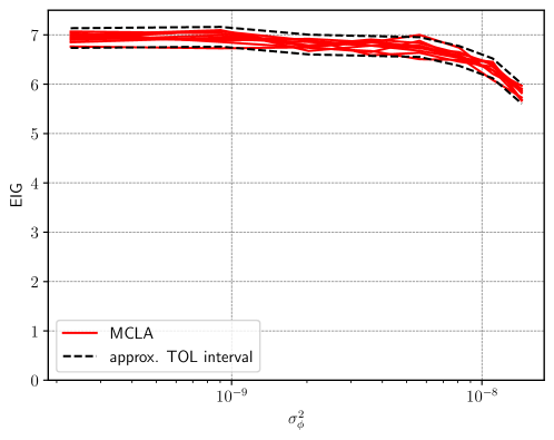
Refer to caption
Figure 1. Example 1: EIG vs. σϕ2superscriptsubscript𝜎italic-ϕ2\sigma_{\phi}^{2} for 10 runs of the MCLA estimator with approximate tolerance interval. The covariance matrix in (20) loses positive definiteness when σϕ2superscriptsubscript𝜎italic-ϕ2\sigma_{\phi}^{2} exceeds a certain threshold of approximately 1.44×1081.44superscript1081.44\times 10^{-8}.

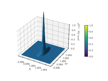
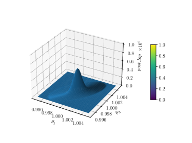
The posterior covariance matrix computed from the MCLA estimator depends on the magnitude of the nuisance uncertainty σϕ2superscriptsubscript𝜎italic-ϕ2\sigma_{\phi}^{2} as indicated in Figure 2. We present the Gaussian posterior pdf once for small σϕ2=1.44×10¹⁶superscriptsubscript𝜎italic-ϕ21.44superscript1016\sigma_{\phi}^{2}=1.44\times 10^{-16} and once for larger σϕ2=1.44×10⁸superscriptsubscript𝜎italic-ϕ21.44superscript108\sigma_{\phi}^{2}=1.44\times 10^{-8} where the small-noise approximation starts breaking down. Naturally, we obtain a more concentrated posterior for the smaller nuisance uncertainty, meaning that the experiment is more informative in the absence of nuisance uncertainty.
Refer to caption
(A) Small σϕ2superscriptsubscript𝜎italic-ϕ2\sigma_{\phi}^{2}
Refer to caption
(B) Large σϕ2superscriptsubscript𝜎italic-ϕ2\sigma_{\phi}^{2}
Figure 2. Example 1: Laplace approximation of the posterior pdf is more concentrated for small nuisance uncertainty σϕ2=1.44×10¹⁶superscriptsubscript𝜎italic-ϕ21.44superscript1016\sigma_{\phi}^{2}=1.44\times 10^{-16} (left) than for a larger nuisance uncertainty σϕ2=1.44×10⁸superscriptsubscript𝜎italic-ϕ21.44superscript108\sigma_{\phi}^{2}=1.44\times 10^{-8} (right).

7.2. Example 2: Linear Gaussian example

The following problem is constructed based on an example by [5], and we use it to assess the efficiency of different estimators because it can be solved analytically. The linear Gaussian example has the form

(72) 𝒈(θ,ϕ)=𝑨𝒛,𝒈𝜃italic-ϕ𝑨𝒛\boldsymbol{g}(\theta,\phi)=\boldsymbol{A}\boldsymbol{z},

where

(73) 𝑨=(ξ00(1ξ)),𝒛=(θϕ),formulae-sequence𝑨matrix𝜉001𝜉𝒛matrix𝜃italic-ϕ\boldsymbol{A}=\begin{pmatrix}\xi&0\\ 0&(1-\xi)\end{pmatrix},\quad\boldsymbol{z}=\begin{pmatrix}\theta\\ \phi\end{pmatrix},

and ϵ𝒩(𝟎,σϵ2𝟏)similar-tobold-italic-ϵ𝒩0superscriptsubscript𝜎italic-ϵ21\boldsymbol{\epsilon}\sim\mathcal{N}(\boldsymbol{0},\sigma_{\epsilon}^{2}\boldsymbol{1}), θ𝒩(0,σθ2)similar-to𝜃𝒩0superscriptsubscript𝜎𝜃2\theta\sim\mathcal{N}(0,\sigma_{\theta}^{2}), ϕ𝒩(0,σϕ2)similar-toitalic-ϕ𝒩0superscriptsubscript𝜎italic-ϕ2\phi\sim\mathcal{N}(0,\sigma_{\phi}^{2}), σϵ2=σϕ2=102superscriptsubscript𝜎italic-ϵ2superscriptsubscript𝜎italic-ϕ2superscript102\sigma_{\epsilon}^{2}=\sigma_{\phi}^{2}=10^{-2}, σθ2=1superscriptsubscript𝜎𝜃21\sigma_{\theta}^{2}=1 and 𝟏1\boldsymbol{1} is the identity matrix in 2superscript2\mathbb{R}^{2}. Alternatively, 𝜽𝜽\boldsymbol{\theta} can be chosen from 2superscript2\mathbb{R}^{2} to observe how the optimal design shifts if there are no nuisance parameters. In this case, 𝒛=𝜽𝒩(𝟎,𝟏)𝒛𝜽similar-to𝒩01\boldsymbol{z}=\boldsymbol{\theta}\sim\mathcal{N}(\boldsymbol{0},\boldsymbol{1}). Figure 3 indicates that both the DLMCIS and MCLA estimator accurately approximate the analytical solution for the case with nuisance parameters and without as long as σϕ2superscriptsubscript𝜎italic-ϕ2\sigma_{\phi}^{2} is kept small enough. As mentioned, if σϕ2superscriptsubscript𝜎italic-ϕ2\sigma_{\phi}^{2} is large, the correction term in the small-noise approximation causes the covariance matrix to lose positive definiteness. In this example, the model 𝒈𝒈\boldsymbol{g} is not bijective for ξ=0𝜉0\xi=0 and ξ=1𝜉1\xi=1. With these design choices, no inference can be made about 𝜽𝜽\boldsymbol{\theta}. The DLMCIS estimator is less robust than the MCLA estimator close to these points.

Refer to captionNo nuisance uncertainty in the EIGWith nuisance uncertainty in the EIG
Figure 3. Example 2: EIG vs. design parameter ξ𝜉\xi. Analytical solution (dashed black), DLMCIS estimator (solid blue), and MCLA estimator (solid red) for the case with or without nuisance uncertainty.

7.2.1. Optimal number of samples and error convergence

Figure 4 depicts the optimal number of outer samples Nsuperscript𝑁N^{\ast} and inner samples Msuperscript𝑀M^{\ast} when computing the EIG for a fixed ξ=1/2𝜉12\xi=1/2. For the DLMC and DLMCIS estimator, the constants CDL,1subscript𝐶DL1C_{\mathrm{DL},1} and CDL,2subscript𝐶DL2C_{\mathrm{DL},2} were estimated using DLMC and DLMCIS, respectively, with N=1000𝑁1000N=1000 and M=200𝑀200M=200. For the MCLA estimator, the constant CLA,1subscript𝐶LA1C_{\mathrm{LA},1} was estimated using MCLA with N=1000𝑁1000N=1000.

The optimal number of inner samples Msuperscript𝑀M^{\ast} for DLMCIS increases at a rate of 𝒪(TOL1)𝒪superscriptTOL1\mathcal{O}(\text{TOL}^{-1}) for small tolerances and is equal to 111 for TOL greater than approximately 101superscript10110^{-1}. The optimal number of outer samples Nsuperscript𝑁N^{\ast} for all three estimators increases at a rate of 𝒪(TOL2)𝒪superscriptTOL2\mathcal{O}(\text{TOL}^{-2}). This holds true for the case with and without nuisance uncertainty. Thus, the total complexity remains unchanged when including nuisance uncertainty into the model.

The absolute error between the true solution and those estimated using MCLA and DLMCIS is presented in Figure 5 for the case with nuisance uncertainty. The previously computed optimal number of samples was used. The consistency test indicates that the absolute error is lower than TOL with 95%percent9595\% probability.

Refer to caption
(A) With nuisance uncertainty
Refer to caption
(B) No nuisance uncertainty
Figure 4. Example 2: Optimal number of outer (Nsuperscript𝑁N^{\ast}) and inner (Msuperscript𝑀M^{\ast}) samples vs. tolerance TOL𝑇𝑂𝐿TOL. Msuperscript𝑀M^{\ast} for the DLMCIS estimator starts increasing for small tolerances.
Refer to caption
(A) DLMCIS
Refer to caption
(B) MCLA
Figure 5. Example 2: Error vs. tolerance consistency plot. Both estimators stay within the allowed tolerance TOL𝑇𝑂𝐿TOL with a predefined confidence parameter Cα=1.96subscript𝐶𝛼1.96C_{\alpha}=1.96 (α=0.05𝛼0.05\alpha=0.05).

7.3. Example 3: Electrical impedance tomography: Recovering fiber orientation in composite laminate materials under nuisance uncertainty

We apply the proposed estimators to EIT, where low-frequency electric currents are injected through electrodes attached to the surface of a closed body to recover the fiber orientation in each orthotropic ply of a composite laminate material based on potential measurements. We adopt the complete electrode model from [19]. The potential field is modeled by a second-order PDE with an electrode boundary model. We assume the exact interior conductivity to be unknown and it is therefore modeled using nuisance parameters. The goal is to determine the design of the experiment, namely, the shift and distance between electrodes, that allows for optimal recovery of the fiber angles under challenging conditions.

7.3.1. EIT formulation

The rectangular body 𝒟𝒟\mathcal{D} with boundary 𝒟𝒟\partial\mathcal{D} consists of two plies 𝒟=i=12𝒟i𝒟superscriptsubscript𝑖12subscript𝒟𝑖\mathcal{D}=\bigcup_{i=1}^{2}\mathcal{D}_{i}. The surfaces of the exterior boundary are equipped with Nelsubscript𝑁elN_{\text{el}} electrodes Elsubscript𝐸𝑙E_{l}, 1lNel1𝑙subscript𝑁el1\leq l\leq N_{\text{el}} with surface impedance zlsubscript𝑧𝑙z_{l}. We have the following PDE formulation

(74) 𝒋(𝒙,ω)=0in𝒟and𝒋𝒙𝜔0in𝒟and\nabla\cdot\boldsymbol{j}(\boldsymbol{x},\omega)=0\quad\text{in}\,\mathcal{D}\,\text{and}
(75) 𝒋(𝒙,ω)=𝝈¯u(𝒙,ω),𝒋𝒙𝜔bold-¯𝝈𝑢𝒙𝜔\boldsymbol{j}(\boldsymbol{x},\omega)=\boldsymbol{\bar{\sigma}}\cdot\nabla u(\boldsymbol{x},\omega),

where u𝑢u is the quasi-static potential field, 𝒋𝒋\boldsymbol{j} indicates the current flux, and 𝝈¯bold-¯𝝈\boldsymbol{\bar{\sigma}} denotes the conductivity field given by

(76) 𝝈¯(𝒙,ω)=𝑸(θi(ω))𝝈(ϕi(ω))𝑸(θi(ω)),for𝒙𝒟i,i=1,2,formulae-sequencebold-¯𝝈𝒙𝜔𝑸superscriptsubscript𝜃𝑖𝜔top𝝈subscriptitalic-ϕ𝑖𝜔𝑸subscript𝜃𝑖𝜔formulae-sequencefor𝒙subscript𝒟𝑖𝑖12\boldsymbol{\bar{\sigma}}(\boldsymbol{x},\omega)=\boldsymbol{Q}(\theta_{i}(\omega))^{\scriptscriptstyle\mskip-1.0mu\top\mskip-2.0mu}\cdot\boldsymbol{\sigma}(\phi_{i}(\omega))\cdot\boldsymbol{Q}(\theta_{i}(\omega)),\quad\text{for}\,\boldsymbol{x}\in\mathcal{D}_{i},\,i=1,2,

where

(77) 𝑸(θi)=(cos(θi)0sin(θi)010sin(θi)0cos(θi))and𝝈(ϕi)=(σ1(ϕi)000σ2(ϕi)000σ3(ϕi)),i=1,2.formulae-sequence𝑸subscript𝜃𝑖matrixsubscript𝜃𝑖0subscript𝜃𝑖010subscript𝜃𝑖0subscript𝜃𝑖andformulae-sequence𝝈subscriptitalic-ϕ𝑖matrixsubscript𝜎1subscriptitalic-ϕ𝑖000subscript𝜎2subscriptitalic-ϕ𝑖000subscript𝜎3subscriptitalic-ϕ𝑖𝑖12\boldsymbol{Q}(\theta_{i})=\begin{pmatrix}\cos(\theta_{i})&0&-\sin(\theta_{i})\\ 0&1&0\\ \sin(\theta_{i})&0&\cos(\theta_{i})\end{pmatrix}\quad\text{and}\quad\boldsymbol{\sigma}(\phi_{i})=\begin{pmatrix}\sigma_{1}(\phi_{i})&0&0\\ 0&\sigma_{2}(\phi_{i})&0\\ 0&0&\sigma_{3}(\phi_{i})\end{pmatrix},\,i=1,2.

The boundary conditions are given by

(78) {𝒋𝒏=0on𝒟(El),El𝒋𝒏dx=IlonEl, 1lNel,1ElEludx+zlEl𝒋𝒏dx=UlonEl, 1lNel,cases𝒋𝒏0on𝒟subscript𝐸𝑙subscriptsubscript𝐸𝑙𝒋𝒏differential-d𝑥subscript𝐼𝑙onsubscript𝐸𝑙1𝑙subscript𝑁el1subscript𝐸𝑙subscriptsubscript𝐸𝑙𝑢differential-d𝑥subscript𝑧𝑙subscriptsubscript𝐸𝑙𝒋𝒏differential-d𝑥subscript𝑈𝑙onsubscript𝐸𝑙1𝑙subscript𝑁el\begin{cases}\boldsymbol{j}\cdot\boldsymbol{n}=0&\text{on}\,\partial\mathcal{D}\setminus(\cup E_{l}),\\ \int_{E_{l}}\boldsymbol{j}\cdot\boldsymbol{n}\,\mathrm{d}{}x=I_{l}&\text{on}\,E_{l},\,1\leq l\leq N_{\text{el}},\\ \frac{1}{E_{l}}\int_{E_{l}}u\,\mathrm{d}{}x+z_{l}\int_{E_{l}}\boldsymbol{j}\cdot\boldsymbol{n}\,\mathrm{d}{}x=U_{l}&\text{on}\,E_{l},\,1\leq l\leq N_{\text{el}},\\ \end{cases}

where 𝒏𝒏\boldsymbol{n} is the unit outward normal. The first one is the no-flux condition, the second one means that the total injected current through each electrode is known and the third one means that the shared interface between electrode and material has an infinitesimally thin layer with surface impedance zlsubscript𝑧𝑙z_{l}. We have the following two constraints (Kirchhoff law of charge conservation and ground potential condition) to guarantee well-posedness:

(79) l=1NelIl=0andl=1NelUl=0.formulae-sequencesuperscriptsubscript𝑙1subscript𝑁elsubscript𝐼𝑙0andsuperscriptsubscript𝑙1subscript𝑁elsubscript𝑈𝑙0\sum_{l=1}^{N_{\text{el}}}I_{l}=0\quad\text{and}\quad\sum_{l=1}^{N_{\text{el}}}U_{l}=0.

The conductivity 𝝈𝝈\boldsymbol{\sigma} must be strictly positive to guarantee coercivity of the bilinear operator. The vector 𝑰=(I1,,INel)𝑰subscript𝐼1subscript𝐼subscript𝑁el\boldsymbol{I}=(I_{1},\ldots,I_{N_{\text{el}}}) provides deterministic injected currents, and the vector 𝑼=(U1,,UNel)𝑼subscript𝑈1subscript𝑈subscript𝑁el\boldsymbol{U}=(U_{1},\ldots,U_{N_{\text{el}}}) provides random measurements of the potential at the electrodes. We solve the system (74), (75) subject to the conditions (78) and (79) for the unknowns (u,𝑼)𝑢𝑼(u,\boldsymbol{U}), which are the potential field on 𝒟𝒟\mathcal{D} and the potential field at the electrodes, respectively.

7.3.2. Experimental design formulation

Ten electrodes are placed on the surface of the rectangular domain 𝒟=[0,20]×[0,2]𝒟02002\mathcal{D}=[0,20]\times[0,2], five on the top, and five on the bottom. The fiber orientations θ1subscript𝜃1\theta_{1} in ply 𝒟1subscript𝒟1\mathcal{D}_{1} and θ2subscript𝜃2\theta_{2} in ply 𝒟2subscript𝒟2\mathcal{D}_{2} are the parameters of interest with the following assumed prior distributions:

(80) θ1π(θ1)=𝒰(π40.05,π4+0.05),θ2π(θ2)=𝒰(π40.05,π4+0.05).formulae-sequencesimilar-tosubscript𝜃1𝜋subscript𝜃1𝒰𝜋40.05𝜋40.05similar-tosubscript𝜃2𝜋subscript𝜃2𝒰𝜋40.05𝜋40.05\theta_{1}\sim\pi(\theta_{1})=\mathcal{U}\left(-\frac{\pi}{4}-0.05,-\frac{\pi}{4}+0.05\right),\quad\theta_{2}\sim\pi(\theta_{2})=\mathcal{U}\left(\frac{\pi}{4}-0.05,\frac{\pi}{4}+0.05\right).

The orthotropic conductivity 𝝈𝝈\boldsymbol{\sigma} is given by

(81) σj(ϕi)=exp(μj+ϕi),j=1,2,3,i=1,2,formulae-sequencesubscript𝜎𝑗subscriptitalic-ϕ𝑖subscript𝜇𝑗subscriptitalic-ϕ𝑖formulae-sequence𝑗123𝑖12\sigma_{j}(\phi_{i})=\exp(\mu_{j}+\phi_{i}),\quad j=1,2,3,\quad i=1,2,

where ϕi=σϕzisubscriptitalic-ϕ𝑖subscript𝜎italic-ϕsubscript𝑧𝑖\phi_{i}=\sigma_{\phi}z_{i} is considered a nuisance parameter for 𝒛𝒩(𝟎,𝟏)similar-to𝒛𝒩01\boldsymbol{z}\sim\mathcal{N}(\boldsymbol{0},\boldsymbol{1}), corresponding to the two plies. We choose μ1=log(0.1)subscript𝜇10.1\mu_{1}=\log(0.1) and μ2=μ3=log(0.02)subscript𝜇2subscript𝜇30.02\mu_{2}=\mu_{3}=\log(0.02) in (81). Surface impedance is considered fixed at zl=z=0.1subscript𝑧𝑙𝑧0.1z_{l}=z=0.1 for each 1lNel1𝑙subscript𝑁el1\leq l\leq N_{\rm{el}} to account for imperfections when attaching the electrodes so that a slight difference can exist between the potential fields at the electrodes. The data model is given by (1) as follows:

(82) 𝒚i=𝒈h(𝜽,ϕ)+ϵi,for 1iNe,formulae-sequencesubscript𝒚𝑖subscript𝒈𝜽bold-italic-ϕsubscriptbold-italic-ϵ𝑖for1𝑖subscript𝑁𝑒\boldsymbol{y}_{i}=\boldsymbol{g}_{h}(\boldsymbol{\theta},\boldsymbol{\phi})+\boldsymbol{\epsilon}_{i},\quad\text{for}\,1\leq i\leq N_{e},

where each 𝒚iqsubscript𝒚𝑖superscript𝑞\boldsymbol{y}_{i}\in\mathbb{R}^{q}, q=Nel1𝑞subscript𝑁el1q=N_{\text{el}}-1 because one electrode is determined by (79). The error distribution is Gaussian, where ϵi𝒩(0,104𝟏q×q).similar-tosubscriptbold-italic-ϵ𝑖𝒩0superscript104subscript1𝑞𝑞\boldsymbol{\epsilon}_{i}\sim\mathcal{N}(0,10^{-4}\boldsymbol{1}_{q\times q}). We consider ten repetitions of the same experiment, so Ne=10subscript𝑁𝑒10N_{e}=10. Moreover, 𝒈h𝑼h=(U1,,UNel1)subscript𝒈subscript𝑼subscript𝑈1subscript𝑈subscript𝑁el1\boldsymbol{g}_{h}\equiv\boldsymbol{U}_{h}=(U_{1},\ldots,U_{N_{\text{el}}-1}) is given by a finite element approximation of 𝑼𝑼\boldsymbol{U} in the Galerkin sense. For details on the finite element formulation, see Appendix C (see Figure 6).

Refer to caption
(A) Domain 𝒟𝒟\mathcal{D} consists of two plies
Refer to caption
(B) Magnitude of the current and current streamlines
Figure 6. Example 3: Panel LABEL:sub@subfig-1:domain.ply Domain 𝒟𝒟\mathcal{D}. Panel LABEL:sub@subfig-2:grad.ply Current streamlines on top of the magnitude of the current. Inlet: red electrodes. Outlet: blue electrodes.

7.3.3. Numerical results

As mentioned, the small-noise approximation breaks down as the updated covariance matrix (20) stops being positive definite for σϕ2superscriptsubscript𝜎italic-ϕ2\sigma_{\phi}^{2} larger than 9.03×1079.03superscript1079.03\times 10^{-7} in the EIT example. Figure 7 illustrates ten runs of the MCLA estimator with the error tolerance specified at TOL=0.2𝑇𝑂𝐿0.2TOL=0.2. Evaluating the forward model 𝑼h(𝜽,ϕ)subscript𝑼𝜽bold-italic-ϕ\boldsymbol{U}_{h}(\boldsymbol{\theta},\boldsymbol{\phi}) for several values of 𝜽𝜽\boldsymbol{\theta} and ϕbold-italic-ϕ\boldsymbol{\phi} shows that results are approximately in the interval [1,9]19[1,9] in absolute value. From (82), we can see that ϵbold-italic-ϵ\boldsymbol{\epsilon} has standard deviation 102superscript10210^{-2}. The relative error in the data coming from the experimental noise is therefore between 0.1%1%percent0.1percent10.1\%-1\%. As for the norm of the gradient, we have ϕ𝒈(𝜽,𝟎)2=𝒪(10)subscriptdelimited-∥∥subscriptbold-italic-ϕ𝒈𝜽02𝒪10\lVert\nabla_{\boldsymbol{\phi}}\boldsymbol{g}(\boldsymbol{\theta},\boldsymbol{0})\rVert_{2}=\mathcal{O}(10), so Remark 3 suggests that the small-noise approximation is applicable for 𝝈ϕ103subscript𝝈bold-italic-ϕsuperscript103\boldsymbol{\sigma}_{\boldsymbol{\phi}}\lessapprox 10^{-3}, in accordance with the results presented in Figure 7. Comparing the posterior covariance matrix for small and large nuisance uncertainty yields similar results as the ones presented in 2, so we omitted them for brevity.
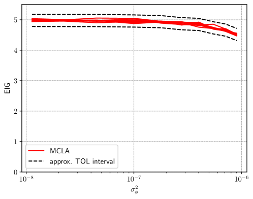
Refer to caption
Figure 7. Example 3: EIG vs. σϕ2superscriptsubscript𝜎italic-ϕ2\sigma_{\phi}^{2} for ten runs of the MCLA estimator with approximate tolerance interval. Covariance matrix in (20) loses positive definiteness when σϕ2superscriptsubscript𝜎italic-ϕ2\sigma_{\phi}^{2} exceeds a certain threshold of approximately 9.03×1079.03superscript1079.03\times 10^{-7}.

Figure 8 reveals the optimal number of outer (Nsuperscript𝑁N^{\ast}) and inner (Msuperscript𝑀M^{\ast}) samples for the DLMC, DLMCIS, and MCLA estimators for a fixed 𝝃=(2,2)𝝃22\boldsymbol{\xi}=(2,2), see Figure 11, and σϕ2=1010superscriptsubscript𝜎italic-ϕ2superscript1010\sigma_{\phi}^{2}=10^{-10}. The constants CDL,1subscript𝐶DL1C_{\mathrm{DL},1}, CDL,2subscript𝐶DL2C_{\mathrm{DL},2} and CDL,4subscript𝐶DL4C_{\mathrm{DL},4} for the DLMC estimator were estimated using DLMC with N=50𝑁50N=50 and M=30𝑀30M=30. For the DLMCIS estimator, these constants were estimated using DLMCIS with N=50𝑁50N=50 and M=10𝑀10M=10 instead. Fewer inner samples are required in the latter case because of importance sampling. Finally, the constants CLA,1subscript𝐶LA1C_{\mathrm{LA},1} and CLA,2subscript𝐶LA2C_{\mathrm{LA},2} for the MCLA estimator were estimated using MCLA with N=50𝑁50N=50. Because of importance sampling, the DLMCIS estimator only requires one inner sample in the optimal setting, except for small tolerances. The MCLA estimator cannot handle small tolerances as the inherent bias becomes greater than the total allowed tolerance, as in Figure 9, where we demonstrate the splitting parameter between the bias and variance error. The error vs. tolerance consistency plot in Figure 10 indicates that the MCLA estimator is consistent and could even handle a coarser mesh. This likely results from an overestimation of the constants η𝜂\eta and CLA,3subscript𝐶LA3C_{\mathrm{LA},3} in (65).

Refer to caption
Figure 8. Example 3: Optimal number of outer (Nsuperscript𝑁N^{\ast}) and inner (Msuperscript𝑀M^{\ast}) samples as a function of the tolerance TOL𝑇𝑂𝐿TOL. The MCLA approximation cannot achieve accuracy when the inherent bias becomes greater than the desired tolerance, and Msuperscript𝑀M^{\ast} for the DLMCIS estimator increases for small tolerances.
Refer to caption
Figure 9. Example 3: The optimal splitting parameter κsuperscript𝜅\kappa^{\ast} is constant for the DLMC and DLMCIS estimators for a small tolerance TOL𝑇𝑂𝐿TOL. The MCLA estimator is infeasible for tolerances smaller than the inherent bias controlled by the number of repetitive experiments Nesubscript𝑁𝑒N_{e}, see (63).
Refer to caption
Figure 10. Example 3: Error vs. tolerance consistency plot. The MCLA estimator stays within the allowed tolerance TOL𝑇𝑂𝐿TOL with a predefined confidence parameter Cα=1.96subscript𝐶𝛼1.96C_{\alpha}=1.96 (α=0.05𝛼0.05\alpha=0.05).

In Figure 11, we present the dependence of the EIG on the design parameters ξ1subscript𝜉1\xi_{1} and ξ2subscript𝜉2\xi_{2}, signifying the shift between the top and bottom electrodes and the distance between the electrodes, respectively, via the MCLA estimator. The setup is optimal for both large ξ1subscript𝜉1\xi_{1} and large ξ2subscript𝜉2\xi_{2}; however, the shift between electrodes seems to have a much greater influence on the EIG than the distance between electrodes.
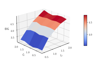
Refer to caption
Figure 11. Example 3: Expected information gain as a function of the design parameters ξ1subscript𝜉1\xi_{1} (the shift between top and bottom electrodes) and ξ2subscript𝜉2\xi_{2} (the distance between electrodes) for the MCLA estimator.

8. Conclusion

We propose two estimators that incorporate nuisance uncertainty in the data model: the MCLA estimator based on a Laplace approximation of the inner integral and the DLMCIS estimator based on importance sampling. Both of these estimators use the small-noise approximation to deal with nuisance uncertainty in a computationally tractable manner. We found that these estimators can accurately approximate the EIG functional for analytical and physical examples as long as the nuisance uncertainty is small enough. This limitation is justified by only considering those parameters that are not primarily responsible for the overall uncertainty of the model as nuisance parameters. Furthermore, we also demonstrated that including the small-noise approximation in the estimators does not affect their analytical error convergence derived in previous work [2].

9. Acknowledgments

This publication is based upon work supported by the King Abdullah University of Science and Technology (KAUST) Office of Sponsored Research (OSR) under Award No. OSR-2019-CRG8-4033, the Alexander von Humboldt Foundation, the Deutsche Forschungsgemeinschaft (DFG, German Research Foundation) – 333849990/GRK2379 (IRTG Modern Inverse Problems), and was partially supported by the Flexible Interdisciplinary Research Collaboration Fund at the University of Nottingham Project ID 7466664.

Appendix A Derivation of the work for two inner loops

The average computational work of the DLMC estimator with two inner loops (9) is given by the solution of the optimization problem

(83) (N,M1,M2)=argmin(N,M1,M2)N(M1+M2)subject toC1M1+C2M2TOL,formulae-sequencesuperscript𝑁superscriptsubscript𝑀1superscriptsubscript𝑀2subscriptargmin𝑁subscript𝑀1subscript𝑀2𝑁subscript𝑀1subscript𝑀2subject tosubscript𝐶1subscript𝑀1subscript𝐶2subscript𝑀2𝑇𝑂𝐿(N^{\ast},M_{1}^{\ast},M_{2}^{\ast})=\operatorname*{arg\,min}_{(N,M_{1},M_{2})}N(M_{1}+M_{2})\quad\text{subject to}\quad\frac{C_{1}}{M_{1}}+\frac{C_{2}}{M_{2}}\leq TOL,

where C1=𝕍[p(𝒀|𝜽,ϕ)|𝒀,𝜽]subscript𝐶1𝕍delimited-[]conditional𝑝conditional𝒀𝜽bold-italic-ϕ𝒀𝜽C_{1}=\mathbb{V}[p(\boldsymbol{Y}|\boldsymbol{\theta},\boldsymbol{\phi})|\boldsymbol{Y},\boldsymbol{\theta}], C2=𝕍[p(𝒀|𝜽,ϕ)|𝒀]subscript𝐶2𝕍delimited-[]conditional𝑝conditional𝒀𝜽bold-italic-ϕ𝒀C_{2}=\mathbb{V}[p(\boldsymbol{Y}|\boldsymbol{\theta},\boldsymbol{\phi})|\boldsymbol{Y}] and TOL𝑇𝑂𝐿TOL is the required tolerance. The derivation of the constants C1subscript𝐶1C_{1} and C2subscript𝐶2C_{2} follows from a simimlar argument as in [2]. Using the method of Lagrange multipliers, we obtain the equation

(84) (N,M1,M2)=N(M1+M2)λ(C1M1+C2M2TOL)𝑁subscript𝑀1subscript𝑀2𝑁subscript𝑀1subscript𝑀2𝜆subscript𝐶1subscript𝑀1subscript𝐶2subscript𝑀2𝑇𝑂𝐿\mathcal{L}(N,M_{1},M_{2})=N(M_{1}+M_{2})-\lambda\left(\frac{C_{1}}{M_{1}}+\frac{C_{2}}{M_{2}}-TOL\right)

with partial derivatives

(85) M1=N+λC1M12subscript𝑀1𝑁𝜆subscript𝐶1superscriptsubscript𝑀12\frac{\partial\mathcal{L}}{\partial M_{1}}=N+\frac{\lambda C_{1}}{M_{1}^{2}}

and

(86) M2=N+λC2M22.subscript𝑀2𝑁𝜆subscript𝐶2superscriptsubscript𝑀22\frac{\partial\mathcal{L}}{\partial M_{2}}=N+\frac{\lambda C_{2}}{M_{2}^{2}}.

Setting these to zero immediately gives

(87) M2=C2C1M1.subscript𝑀2subscript𝐶2subscript𝐶1subscript𝑀1M_{2}=\sqrt{\frac{C_{2}}{C_{1}}}M_{1}.

From the partial derivative

(88) λ=C1M1+C2M2TOL,𝜆subscript𝐶1subscript𝑀1subscript𝐶2subscript𝑀2𝑇𝑂𝐿\frac{\partial\mathcal{L}}{\partial\lambda}=\frac{C_{1}}{M_{1}}+\frac{C_{2}}{M_{2}}-TOL,

set to zero, we obtain that

(89) TOL=C1+C1C2M1.𝑇𝑂𝐿subscript𝐶1subscript𝐶1subscript𝐶2subscript𝑀1TOL=\frac{C_{1}+\sqrt{C_{1}C_{2}}}{M_{1}}.

Thus, we have that

(90) M1+M2=C1+2C1C2+C2TOL.subscript𝑀1subscript𝑀2subscript𝐶12subscript𝐶1subscript𝐶2subscript𝐶2𝑇𝑂𝐿M_{1}+M_{2}=\frac{C_{1}+2\sqrt{C_{1}C_{2}}+C_{2}}{TOL}.

Appendix B Derivation of the order of the maximum a posteriori approximation

Let

S(𝜽)𝑆𝜽\displaystyle S(\boldsymbol{\theta}) =12Ne(𝒈(𝜽t,𝟎)𝒈(𝜽,𝟎))𝚺ϵ1/2𝑪(𝜽)𝚺ϵ1/2(𝒈(𝜽t,𝟎)𝒈(𝜽,𝟎))absent12subscript𝑁𝑒superscript𝒈subscript𝜽𝑡0𝒈𝜽0topsuperscriptsubscript𝚺bold-italic-ϵ12𝑪𝜽superscriptsubscript𝚺bold-italic-ϵ12𝒈subscript𝜽𝑡0𝒈𝜽0\displaystyle=\frac{1}{2}N_{e}(\boldsymbol{g}(\boldsymbol{\theta}_{t},\boldsymbol{0})-\boldsymbol{g}(\boldsymbol{\theta},\boldsymbol{0}))^{\scriptscriptstyle\mskip-1.0mu\top\mskip-2.0mu}\boldsymbol{\Sigma}_{\boldsymbol{\epsilon}}^{-1/2}\boldsymbol{C}(\boldsymbol{\theta})\boldsymbol{\Sigma}_{\boldsymbol{\epsilon}}^{-1/2}(\boldsymbol{g}(\boldsymbol{\theta}_{t},\boldsymbol{0})-\boldsymbol{g}(\boldsymbol{\theta},\boldsymbol{0}))
(91) +i=1Neϵi𝚺ϵ1/2𝑪(𝜽)𝚺ϵ1/2(𝒈(𝜽t,𝟎)𝒈(𝜽,𝟎))h(𝜽)+D(𝜽)superscriptsubscript𝑖1subscript𝑁𝑒subscriptbold-italic-ϵ𝑖superscriptsubscript𝚺bold-italic-ϵ12𝑪𝜽superscriptsubscript𝚺bold-italic-ϵ12𝒈subscript𝜽𝑡0𝒈𝜽0𝜽𝐷𝜽\displaystyle+\sum_{i=1}^{N_{e}}\boldsymbol{\epsilon}_{i}\boldsymbol{\Sigma}_{\boldsymbol{\epsilon}}^{-1/2}\boldsymbol{C}(\boldsymbol{\theta})\boldsymbol{\Sigma}_{\boldsymbol{\epsilon}}^{-1/2}(\boldsymbol{g}(\boldsymbol{\theta}_{t},\boldsymbol{0})-\boldsymbol{g}(\boldsymbol{\theta},\boldsymbol{0}))-h(\boldsymbol{\theta})+D(\boldsymbol{\theta})

with gradient

𝜽S(𝜽)subscript𝜽𝑆𝜽\displaystyle\nabla_{\boldsymbol{\theta}}S(\boldsymbol{\theta}) =Ne𝜽𝒈(𝜽,𝟎)𝚺ϵ1/2𝑪(𝜽)𝚺ϵ1/2(𝒈(𝜽t,𝟎)𝒈(𝜽,𝟎))absentsubscript𝑁𝑒subscript𝜽𝒈𝜽0superscriptsubscript𝚺bold-italic-ϵ12𝑪𝜽superscriptsubscript𝚺bold-italic-ϵ12𝒈subscript𝜽𝑡0𝒈𝜽0\displaystyle=-N_{e}\nabla_{\boldsymbol{\theta}}\boldsymbol{g}(\boldsymbol{\theta},\boldsymbol{0})\boldsymbol{\Sigma}_{\boldsymbol{\epsilon}}^{-1/2}\boldsymbol{C}(\boldsymbol{\theta})\boldsymbol{\Sigma}_{\boldsymbol{\epsilon}}^{-1/2}(\boldsymbol{g}(\boldsymbol{\theta}_{t},\boldsymbol{0})-\boldsymbol{g}(\boldsymbol{\theta},\boldsymbol{0}))
+Ne(𝒈(𝜽t,𝟎)𝒈(𝜽,𝟎))𝚺ϵ1/2𝜽𝑪(𝜽)𝚺ϵ1/2(𝒈(𝜽t,𝟎)𝒈(𝜽,𝟎))subscript𝑁𝑒superscript𝒈subscript𝜽𝑡0𝒈𝜽0topsuperscriptsubscript𝚺bold-italic-ϵ12subscript𝜽𝑪𝜽superscriptsubscript𝚺bold-italic-ϵ12𝒈subscript𝜽𝑡0𝒈𝜽0\displaystyle+N_{e}(\boldsymbol{g}(\boldsymbol{\theta}_{t},\boldsymbol{0})-\boldsymbol{g}(\boldsymbol{\theta},\boldsymbol{0}))^{\scriptscriptstyle\mskip-1.0mu\top\mskip-2.0mu}\boldsymbol{\Sigma}_{\boldsymbol{\epsilon}}^{-1/2}\nabla_{\boldsymbol{\theta}}\boldsymbol{C}(\boldsymbol{\theta})\boldsymbol{\Sigma}_{\boldsymbol{\epsilon}}^{-1/2}(\boldsymbol{g}(\boldsymbol{\theta}_{t},\boldsymbol{0})-\boldsymbol{g}(\boldsymbol{\theta},\boldsymbol{0}))
i=1Neϵi𝚺ϵ1/2𝑪(𝜽)𝚺ϵ1/2𝜽𝒈(𝜽,𝟎)superscriptsubscript𝑖1subscript𝑁𝑒subscriptbold-italic-ϵ𝑖superscriptsubscript𝚺bold-italic-ϵ12𝑪𝜽superscriptsubscript𝚺bold-italic-ϵ12subscript𝜽𝒈𝜽0\displaystyle-\sum_{i=1}^{N_{e}}\boldsymbol{\epsilon}_{i}\boldsymbol{\Sigma}_{\boldsymbol{\epsilon}}^{-1/2}\boldsymbol{C}(\boldsymbol{\theta})\boldsymbol{\Sigma}_{\boldsymbol{\epsilon}}^{-1/2}\nabla_{\boldsymbol{\theta}}\boldsymbol{g}(\boldsymbol{\theta},\boldsymbol{0})
(92) +i=1Neϵi𝚺ϵ1/2𝜽𝑪(𝜽)𝚺ϵ1/2(𝒈(𝜽t,𝟎)𝒈(𝜽,𝟎))𝜽h(𝜽)+𝜽D(𝜽),superscriptsubscript𝑖1subscript𝑁𝑒subscriptbold-italic-ϵ𝑖superscriptsubscript𝚺bold-italic-ϵ12subscript𝜽𝑪𝜽superscriptsubscript𝚺bold-italic-ϵ12𝒈subscript𝜽𝑡0𝒈𝜽0subscript𝜽𝜽subscript𝜽𝐷𝜽\displaystyle+\sum_{i=1}^{N_{e}}\boldsymbol{\epsilon}_{i}\boldsymbol{\Sigma}_{\boldsymbol{\epsilon}}^{-1/2}\nabla_{\boldsymbol{\theta}}\boldsymbol{C}(\boldsymbol{\theta})\boldsymbol{\Sigma}_{\boldsymbol{\epsilon}}^{-1/2}(\boldsymbol{g}(\boldsymbol{\theta}_{t},\boldsymbol{0})-\boldsymbol{g}(\boldsymbol{\theta},\boldsymbol{0}))-\nabla_{\boldsymbol{\theta}}h(\boldsymbol{\theta})+\nabla_{\boldsymbol{\theta}}D(\boldsymbol{\theta}),

where 𝜽𝑪=2𝚺ϵ1/2𝜽ϕ𝒈(𝜽,𝟎)𝚺ϕ1/2𝑴𝚺ϵ1/2subscript𝜽𝑪2superscriptsubscript𝚺bold-italic-ϵ12subscript𝜽subscriptbold-italic-ϕ𝒈𝜽0superscriptsubscript𝚺bold-italic-ϕ12superscript𝑴topsuperscriptsubscript𝚺bold-italic-ϵ12\nabla_{\boldsymbol{\theta}}\boldsymbol{C}=-2\boldsymbol{\Sigma}_{\boldsymbol{\epsilon}}^{-1/2}\nabla_{\boldsymbol{\theta}}\nabla_{\boldsymbol{\phi}}\boldsymbol{g}(\boldsymbol{\theta},\boldsymbol{0})\boldsymbol{\Sigma}_{\boldsymbol{\phi}}^{1/2}\boldsymbol{M}^{\scriptscriptstyle\mskip-1.0mu\top\mskip-2.0mu}\boldsymbol{\Sigma}_{\boldsymbol{\epsilon}}^{-1/2}.

Applying Newton’s method and 𝜽S(𝜽^)=𝟎subscript𝜽𝑆^𝜽0\nabla_{\boldsymbol{\theta}}S(\hat{\boldsymbol{\theta}})=\boldsymbol{0} implies that

𝜽S(𝜽t)+𝜽𝜽S(𝜽t)(𝜽^𝜽t)𝟎subscript𝜽𝑆subscript𝜽𝑡subscript𝜽subscript𝜽𝑆subscript𝜽𝑡^𝜽subscript𝜽𝑡0\nabla_{\boldsymbol{\theta}}S(\boldsymbol{\theta}_{t})+\nabla_{\boldsymbol{\theta}}\nabla_{\boldsymbol{\theta}}S(\boldsymbol{\theta}_{t})(\hat{\boldsymbol{\theta}}-\boldsymbol{\theta}_{t})\approx\boldsymbol{0}, so

(93) 𝜽^𝜽t𝜽𝜽S(𝜽t)1𝜽S(𝜽t),bold-^𝜽subscript𝜽𝑡subscript𝜽subscript𝜽𝑆superscriptsubscript𝜽𝑡1subscript𝜽𝑆subscript𝜽𝑡\boldsymbol{\hat{\theta}}\approx\boldsymbol{\theta}_{t}-\nabla_{\boldsymbol{\theta}}\nabla_{\boldsymbol{\theta}}S(\boldsymbol{\theta}_{t})^{-1}\nabla_{\boldsymbol{\theta}}S(\boldsymbol{\theta}_{t}),

providing

(94) 𝜽^𝜽t(Ne𝜽𝒈(𝜽t,𝟎)𝚺ϵ1/2𝑪(𝜽t)𝚺ϵ1/2𝜽𝒈(𝜽t,𝟎)i=1Neϵi𝚺ϵ1/2𝑪(𝜽t)𝚺ϵ1/2𝜽𝜽𝒈(𝜽t,𝟎)2i=1Neϵi𝚺ϵ1/2𝜽𝑪(𝜽t)𝚺ϵ1/2𝜽𝒈(𝜽t,𝟎)𝜽𝜽h(𝜽t)+𝜽𝜽D(𝜽t))1×(i=1Neϵi𝚺ϵ1/2𝑪(𝜽t)𝚺ϵ1/2𝜽𝒈(𝜽t,𝟎)𝜽h(𝜽t)+𝜽D(𝜽t)).bold-^𝜽subscript𝜽𝑡superscriptsubscript𝑁𝑒subscript𝜽𝒈subscript𝜽𝑡0superscriptsubscript𝚺bold-italic-ϵ12𝑪subscript𝜽𝑡superscriptsubscript𝚺bold-italic-ϵ12subscript𝜽𝒈subscript𝜽𝑡0superscriptsubscript𝑖1subscript𝑁𝑒subscriptbold-italic-ϵ𝑖superscriptsubscript𝚺bold-italic-ϵ12𝑪subscript𝜽𝑡superscriptsubscript𝚺bold-italic-ϵ12subscript𝜽subscript𝜽𝒈subscript𝜽𝑡02superscriptsubscript𝑖1subscript𝑁𝑒subscriptbold-italic-ϵ𝑖superscriptsubscript𝚺bold-italic-ϵ12subscript𝜽𝑪subscript𝜽𝑡superscriptsubscript𝚺bold-italic-ϵ12subscript𝜽𝒈subscript𝜽𝑡0subscript𝜽subscript𝜽subscript𝜽𝑡subscript𝜽subscript𝜽𝐷subscript𝜽𝑡1superscriptsubscript𝑖1subscript𝑁𝑒subscriptbold-italic-ϵ𝑖superscriptsubscript𝚺bold-italic-ϵ12𝑪subscript𝜽𝑡superscriptsubscript𝚺bold-italic-ϵ12subscript𝜽𝒈subscript𝜽𝑡0subscript𝜽subscript𝜽𝑡subscript𝜽𝐷subscript𝜽𝑡\boldsymbol{\hat{\theta}}\approx\boldsymbol{\theta}_{t}-\Bigg{(}N_{e}\nabla_{\boldsymbol{\theta}}\boldsymbol{g}(\boldsymbol{\theta}_{t},\boldsymbol{0})\boldsymbol{\Sigma}_{\boldsymbol{\epsilon}}^{-1/2}\boldsymbol{C}(\boldsymbol{\theta}_{t})\boldsymbol{\Sigma}_{\boldsymbol{\epsilon}}^{-1/2}\nabla_{\boldsymbol{\theta}}\boldsymbol{g}(\boldsymbol{\theta}_{t},\boldsymbol{0})-\sum_{i=1}^{N_{e}}\boldsymbol{\epsilon}_{i}\boldsymbol{\Sigma}_{\boldsymbol{\epsilon}}^{-1/2}\boldsymbol{C}(\boldsymbol{\theta}_{t})\boldsymbol{\Sigma}_{\boldsymbol{\epsilon}}^{-1/2}\nabla_{\boldsymbol{\theta}}\nabla_{\boldsymbol{\theta}}\boldsymbol{g}(\boldsymbol{\theta}_{t},\boldsymbol{0})\\ -2\sum_{i=1}^{N_{e}}\boldsymbol{\epsilon}_{i}\boldsymbol{\Sigma}_{\boldsymbol{\epsilon}}^{-1/2}\nabla_{\boldsymbol{\theta}}\boldsymbol{C}(\boldsymbol{\theta}_{t})\boldsymbol{\Sigma}_{\boldsymbol{\epsilon}}^{-1/2}\nabla_{\boldsymbol{\theta}}\boldsymbol{g}(\boldsymbol{\theta}_{t},\boldsymbol{0})-\nabla_{\boldsymbol{\theta}}\nabla_{\boldsymbol{\theta}}h(\boldsymbol{\theta}_{t})+\nabla_{\boldsymbol{\theta}}\nabla_{\boldsymbol{\theta}}D(\boldsymbol{\theta}_{t})\Bigg{)}^{-1}\\ \times\left(-\sum_{i=1}^{N_{e}}\boldsymbol{\epsilon}_{i}\boldsymbol{\Sigma}_{\boldsymbol{\epsilon}}^{-1/2}\boldsymbol{C}(\boldsymbol{\theta}_{t})\boldsymbol{\Sigma}_{\boldsymbol{\epsilon}}^{-1/2}\nabla_{\boldsymbol{\theta}}\boldsymbol{g}(\boldsymbol{\theta}_{t},\boldsymbol{0})-\nabla_{\boldsymbol{\theta}}h(\boldsymbol{\theta}_{t})+\nabla_{\boldsymbol{\theta}}D(\boldsymbol{\theta}_{t})\right).

The leading order term in the denominator is of order 𝒪(Ne𝚺ϕ)subscript𝒪subscript𝑁𝑒delimited-∥∥subscript𝚺bold-italic-ϕ\mathcal{O}_{\mathbb{P}}\left(N_{e}\lVert\boldsymbol{\Sigma}_{\boldsymbol{\phi}}\rVert\right), and the leading order term in the numerator is of order 𝒪(Ne𝚺ϕ)subscript𝒪subscript𝑁𝑒delimited-∥∥subscript𝚺bold-italic-ϕ\mathcal{O}_{\mathbb{P}}\left(\sqrt{N_{e}}\lVert\boldsymbol{\Sigma}_{\boldsymbol{\phi}}\rVert\right), so we have 𝜽^=𝜽t+𝒪(1Ne)bold-^𝜽subscript𝜽𝑡subscript𝒪1subscript𝑁𝑒\boldsymbol{\hat{\theta}}=\boldsymbol{\theta}_{t}+\mathcal{O}_{\mathbb{P}}\left(\frac{1}{\sqrt{N_{e}}}\right) as Nesubscript𝑁𝑒N_{e}\rightarrow\infty.

Appendix C Derivation of the finite element formulation

Let (Ω,,)Ω(\Omega,\mathcal{F},\mathbb{P}) be a complete probability space with a set of outcomes ΩΩ\Omega, σ𝜎\sigma-field \mathcal{F}, and probability measure \mathbb{P}. We define H1(𝒟×Nel)superscript𝐻1𝒟superscriptsubscript𝑁el\mathcal{H}\coloneqq H^{1}(\mathcal{D}\times\mathbb{R}^{N_{\rm{el}}}) as the space of the solution for the potential field (u(ω),𝑼(ω))𝑢𝜔𝑼𝜔(u(\omega),\boldsymbol{U}(\omega)) for ωΩ𝜔Ω\omega\in\Omega and the Bochner space L2(Ω;)superscriptsubscript𝐿2ΩL_{\mathbb{P}}^{2}(\Omega;\mathcal{H}) as

(95) L2(Ω;){(u,𝑼):Ωs.t.Ω(u(ω),𝑼(ω))2d(ω)<}.superscriptsubscript𝐿2Ωconditional-set𝑢𝑼formulae-sequenceΩs.t.subscriptΩsuperscriptsubscriptdelimited-∥∥𝑢𝜔𝑼𝜔2differential-d𝜔L_{\mathbb{P}}^{2}(\Omega;\mathcal{H})\coloneqq\left\{(u,\boldsymbol{U}):\Omega\to\mathcal{H}\quad\text{s.t.}\,\int_{\Omega}\lVert(u(\omega),\boldsymbol{U}(\omega))\rVert_{\mathcal{H}}^{2}\,\mathrm{d}{}\mathbb{P}(\omega)<\infty\right\}.

For the bilinear form B:×:𝐵B:\mathcal{H}\times\mathcal{H}\to\mathbb{R}, given as

(96) B((u,𝑼),(v,𝑽))𝒟𝒋vd𝒟+l=1Nel1zlEl(𝑼lu)(𝑽lv)dEl,𝐵𝑢𝑼𝑣𝑽subscript𝒟𝒋𝑣d𝒟superscriptsubscript𝑙1subscript𝑁el1subscript𝑧𝑙subscriptsubscript𝐸𝑙subscript𝑼𝑙𝑢subscript𝑽𝑙𝑣differential-dsubscript𝐸𝑙B((u,\boldsymbol{U}),(v,\boldsymbol{V}))\coloneqq\int_{\mathcal{D}}\boldsymbol{j}\cdot\nabla v\,\mathrm{d}{}\mathcal{D}+\sum_{l=1}^{N_{\rm{el}}}\frac{1}{z_{l}}\int_{E_{l}}(\boldsymbol{U}_{l}-u)(\boldsymbol{V}_{l}-v)\,\mathrm{d}{}E_{l},

we aim to determine (u,𝑼)L2(Ω;)𝑢𝑼superscriptsubscript𝐿2Ω(u,\boldsymbol{U})\in L_{\mathbb{P}}^{2}(\Omega;\mathcal{H}) such that the weak formulation

(97) 𝔼[B((u,𝑼),(v,𝑽))]=𝑰e𝔼[𝑼]𝔼delimited-[]𝐵𝑢𝑼𝑣𝑽subscript𝑰𝑒𝔼delimited-[]𝑼\mathbb{E}[B((u,\boldsymbol{U}),(v,\boldsymbol{V}))]=\boldsymbol{I}_{e}\cdot\mathbb{E}[\boldsymbol{U}]

is fulfilled for all (v,𝑽)L2(Ω;)𝑣𝑽superscriptsubscript𝐿2Ω(v,\boldsymbol{V})\in L_{\mathbb{P}}^{2}(\Omega;\mathcal{H}).

References

  • [1] Ryan KJ. Estimating expected information gains for experimental designs with application to the random fatigue-limit model. Journal of Computational and Graphical Statistics, 12:585–603, 2003.
  • [2] Beck J, Dia BM, Espath LF, Long Q, and Tempone R. Fast Bayesian experimental design: Laplace-based importance sampling for the expected information gain. Computer Methods in Applied Mechanics and Engineering, 334:523–553, 2018.
  • [3] Beck J, Dia BM, Espath LF, and Tempone R. Multilevel double loop Monte Carlo and stochastic collocation methods with importance sampling for Bayesian optimal experimental design. International Journal for Numerical Methods in Engineering, 121:3482–3503, 2020.
  • [4] Carlon AG, Dia BM, Espath LF, Lopez RH, and Tempone R. Nesterov-aided stochastic gradient methods using Laplace approximation for Bayesian design optimization. Computer Methods in Applied Mechanics and Engineering, 363:112909, 2020.
  • [5] Feng C and Marzouk YM. A layered multiple importance sampling scheme for focused optimal Bayesian experimental design. arXiv preprint arXiv:1903.11187, 2019.
  • [6] Alexanderian A, Petra N, Stadler G, and Sunseri I. Optimal design of large-scale Bayesian linear inverse problems under reducible model uncertainty: good to know what you don’t know. arXiv preprint arXiv:2006.11939, 2020.
  • [7] Shannon CE. A mathematical theory of communication. Bell System Technical Journal, 27:379–423, 1948.
  • [8] Kullback S. Information theory and statistics. Wiley, 1959.
  • [9] Long Q, Scavino M, Tempone R, and Wang S. Fast estimation of expected information gains for Bayesian experimental designs based on Laplace approximations. Computer Methods in Applied Mechanics and Engineering, 259:24–39, 2013.
  • [10] Long Q. Multimodal information gain in Bayesian design of experiments. arXiv preprint arXiv:2108.07224, 2021.
  • [11] Bernardo JM. Reference posterior distributions for Bayesian inference. Journal of the Royal Statistical Society, Series B 41, 1979.
  • [12] Schillings C, Sprungk B, and Wacker P. On the convergence of the Laplace approximation and noise-level-robustness of Laplace-based Monte Carlo methods for Bayesian inverse problems. Numerische Mathematik, 145:915–971, 2020.
  • [13] Wacker P. Laplace’s method in Bayesian inverse problems. arXiv preprint arXiv:1701.07989, 2017.
  • [14] Polson NG. Bayesian Perspectives on Statistical Modelling. Ph.D. thesis, Department of Mathematics, University of Nottingham, 1988.
  • [15] Liepe J, Filippi S, Komorowski M, and Stumpf MPH. Maximizing the information content of experiments in systems biology. PLOS Computational Biology, 9:1–13, 2013.
  • [16] Chaloner K and Verdinelli I. Bayesian experimental design: a review. Statistical Sciences, 10:273–304, 1995.
  • [17] Kullback S and Leibler RA. On information and sufficiency. Annals of Mathematical Statistics, 22:79–86, 1951.
  • [18] Stigler SM. Laplace’s 1774 memoir on inverse probability. Statistical Science, 1:359–378, 1986.
  • [19] Somersalo E, Cheney M, and Isaacson D. Existence and uniqueness for electrode models for electric current computed tomography. SIAM Journal on Applied Mathematics, 52:1023–1040, 1992.
  • [20] Lindley DV. On a measure of information provided by an experiment. Annals of Mathematical Statistics, 27:986–1005, 1956.
  • [21] Tierney L and Kadane JB. Accurate approximations for posterior moments and marginal densities. Journal of the American Statistical Association, 81:82–86, 1986.
  • [22] Tierney L, Kass RE, and Kadane JB. Fully exponential Laplace approximations to expectations and variances of nonpositive functions. Journal of the American Statistical Association, 84:710–716, 1989.
  • [23] Kass RE, Tierney L, and Kadane JB. The validity of posterior expansions based on Laplace’s method. in: Geisser S, Hodges JS, Press SJ, and Zellner A (Eds.), Essays in Honor of George Barnard, 473–488, 1990.
  • [24] Long Q, Scavino M, Tempone R, and Wang S. A Laplace method for under-determined Bayesian optimal experimental designs. Computer Methods in Applied Mechanics and Engineering, 285:849–876, 2015.
  • [25] Levine DS. Focused active inference. Ph.D. thesis, Department of Aeronautics and Astronautics, Massachusetts Institute of Technology, 2014.
  • [26] Kennedy M and O’Hagan A. Bayesian calibration of computer models. Journal of the Royal Statistical Society, 63:425–464, 2001.
  • [27] Long Q, Motamed M, and Tempone R. Fast Bayesian optimal experimental design for seismic source inversion. Computer Methods in Applied Mechanics and Engineering, 291:123–145, 2015.
  • [28] Bisetti F, Kim D, Knio O, Long Q, and Tempone R. Optimal Bayesian experimental design for priors of compact support with application to shock-tube experiments for combustion kinetics. International Journal for Numerical Methods in Engineering, 108:136–155, 2016.
  • [29] Helin T, and Kretschmann R. Non-asymptotic error estimates for the Laplace approximation in Bayesian inverse problems. Numerische Mathematik, 150:521–549, 2022.
  • [30] Spokoiny V. Dimension free non-asymptotic bounds on the accuracy of high dimensional Laplace approximation. arXiv preprint arXiv:2204.11038, 2022.