Roozbeh Yousefzadeh \Emailroozbeh.yousefzadeh@yale.edu
\addrYale University and VA Connecticut Healthcare System, New Haven, CT, USA
A Homotopy Algorithm for Optimal Transport
Abstract
The optimal transport problem has many applications in machine learning, physics, biology, economics, etc. Although its goal is very clear and mathematically well-defined, finding its optimal solution can be challenging for large datasets in high-dimensional space. Here, we propose a homotopy algorithm that first transforms the problem into an easy form, by changing the target distribution. It then transforms the problem back to the original form through a series of iterations, tracing a path of solutions until it finds the optimal solution for the original problem. We define the homotopy path as a subspace rotation based on the orthogonal Procrustes problem, and then we discretize the homotopy path using eigenvalue decomposition of the rotation matrix. Our goal is to provide an algorithm with complexity bound , faster than the existing methods in the literature.
1 Introduction
The optimal transport problem has been the subject of many studies in recent years as it has several applications in machine learning and other fields, such as physics (Buttazzo et al., 2012), biology (Schiebinger et al., 2019), economics (Galichon, 2018), etc. Study of this problem has, in fact, a long history, going back to the 18th century (Villani, 2008). Although there are well-known algorithms for solving this problem, those algorithms are not practical or fast enough when we deal with modern machine learning datasets with large number of samples and many features (Peyré et al., 2019). In fact, the best known complexity bound for this problem is , for distributions with samples Pele and Werman (2009). In pursuit of faster algorithms, a regularized (relaxed) version of this problem was proposed by Cuturi (2013) and there has been many advances in solving the regularized formulation, e.g., Lin et al. (2020b, a). Here, we design the outline of a homotopy algorithm for the original formulation, suggesting that the optimal solution may be computed with complexity bound . Our algorithm exploits the structure of the data and starts by solving a related problem with known optimal solution. By following a continuous path, it then transforms the related problem back to its original form until it finds the solution for the original problem.
2 Formulation
We would like to find a 1-to-1 mapping from one set of points (a discrete distribution) to another set of points , such that the sum of distances between the matched points is minimal. Each set has discrete points in . In the general form of the problem, the distance between the points can be measured using different metrics (Gramfort et al., 2015). In our formulation, we use the Euclidean distance which is common in the optimal transport literature and is used for analyzing the complexity of most recent algorithms (Lin et al., 2020b, a; Guo et al., 2020). In this setting, each point set can be considered a discrete probability distribution. Using a transportation plan , the goal is to basically transport the discrete distribution to the discrete distribution .
We organize the information about the discrete distributions and in matrix form, where columns represent the points (i.e., samples) and rows represent the dimensions (i.e, features). is a binary matrix that determines the pairwise matching between the points in and . Since the mapping is 1-to-1, the sum of each row and each column of should be equal to 1. Our optimization problem is as following:
| (1) |
subject to:
| (2) |
| (3) |
| (4) |
3 Our homotopy approach
We now design our homotopy algorithm to solve the above formulation. In numerical optimization, homotopy algorithms are usually used to solve hard optimization problems (Nocedal and Wright, 2006). In such approach, a homotopy transformation is designed to overcome the specific challenges of the hard problem. Recent examples of developing homotopy algorithms include (Dunlavy and O’Leary, 2005; Mobahi and Fisher III, 2015; Anandkumar et al., 2017; Yousefzadeh and O’Leary, 2020). In our approach, we transform the target distribution into a distribution such that the solution to our optimization problem (Equations (1)-(4)) is unique and easily computable. We then gradually transform the back to its original form, , through a series of iterations.
3.1 Investigating the formulation
Let’s start by investigating our objective function and find a plausible way to transform it into a state where the optimal solution is known. From linear algebra, it is easy to show that
| (5) |
where is the trace operator. Our objective function is, therefore, equivalent to
3.2 Homotopy transformation
To design a homotopy algorithm, we have to first design a transformation that makes our optimization problem easier to solve. Besides that, we also want the transformed problem to be related to the original problem, so that the solution of transformed problem can lead us to the solution of original problem.
Based on the above considerations, we replace the with , and instead of constraints (2)-(4), we only require the to be orthogonal, i.e., . With such relaxation, we can analytically find its unique optimal solution, . In fact, this relaxation would provide a lower bound to the solution of our minimization problem in Equation (1), which would translate to an upper bound on the solution of our maximization problem in Equation (6). Note that is also orthogonal, so in our transformation, we have preserved that property for . As we will see later, orthogonality of will be helpful in discretizing the homotopy path.
The way to compute the is to compute the SVD of . We can then compute the optimal solution as , as proved in (Golub and Van Loan, 2012, Section 6.4). Now, if we replace our with and set , we have actually optimized our problem for distributions and . This defines our homotopy transformation: transforming to . This transformation is merely a step to make the problem tractable, so we do not need to precisely compute the . Instead, we can use a randomized SVD algorithm to approximate the . The complexity of computing the is therefore, , where is the number of singular values used in the approximation (Halko et al., 2011).
3.3 Homotopy path
The next step is to follow a homotopy path to gradually transform the back to its original form, . At each iteration , moves closer towards , and we optimize the for , using the as the starting point. At the end, we obtain a solution for transporting to .
One can follow different paths to transition back to . Here, we choose a homotopy path that corresponds to the transformation used to obtain the in the first place. The transformation performed with is a subspace rotation, known in linear algebra as the ”orthogonal Procrustes problem”. Since our homotopy is a rotation, we devise a path to gradually reverse the rotation.
We note that is orthogonal and non-singular. Therefore, using a blocked Schur algorithm (Deadman et al., 2012), we can compute its square root, , such that it is a function of . Such square root is guaranteed to exist for and it would also be orthogonal (Higham, 1987; Higham et al., 2005). This breaks our overall rotation into two steps. By computing the square root of , we can then break each of the above two steps into two finer steps, and so on. This way, we can discretize our continuous homotopy path. As an example, if we discretize 3 times, our incremental rotation matrix will be . This corresponds to steps to move from to .
Since the square roots are a function of , our homotopy path is also a function of , and our discretization points will be on a continuous homotopy path. Moreover, since (and its square roots) is orthogonal, its condition number is 1 which is desirable for numerical stability.
We note that following this procedure, the number of steps will be a power of 2. The best step size would be such that the solution at each step is relatively close to the solution from the previous step, so that we can easily move from one solution to another. Making the step sizes very fine can make the process inefficient, as the solution might stay the same between very fine steps.
Regarding the computational complexity, the number of homotopy steps, , is a constant, e.g., 2, 4, 8, or 16. Hence, it does not add to the overall complexity of our algorithm. The complexity of computing the square roots of is equivalent to the complexity of eigenvalue decomposition, .
3.4 Updating the solution along the path
At each iteration on the homotopy path, we aim to improve the solution from the previous step. For that, we use an optimization module
| (7) |
which takes as input the two discrete distributions and a as the initial solution for optimization variables. It then returns as the optimal solution.
Since is a permutation matrix, should be a combinatorial algorithm. There are off-the-shelf exact and approximation algorithms for . Since we are following a homotopy path, we expect the optimal solution at each iteration to be relatively similar to the previous iteration. Therefore, we can rely on efficient algorithms that only aim to improve the solution by making local modifications to it. For example, Duan and Pettie (2014) and Altschuler et al. (2017) perform local updates in near-linear time with approximation guarantees.
Comprehensive options for aim to optimize the globally, e.g. Duff and Koster (2001). We use them to verify our results and to ensure that our local updates are adequate. Algorithm 1 formalizes these procedures.
Inputs: Discrete distribution , target distribution , number of homotopy steps (power of 2)
Outputs: Transport plan , total transport cost
in Algorithm 1 basically performs a pass over the samples in . For each sample in , it assigns the closest unassigned sample in , until it has a 1-to-1 matching between the points in and . This has complexity and it is a quick and efficient attempt to initialize the transportation plan.
We note that the homotopy transformation has overall complexity of . The process of updating the optimal solutions along the homotopy path can also be performed in using approximation algorithms for , leading to overall complexity of for Algorithm 1.
4 Toy example
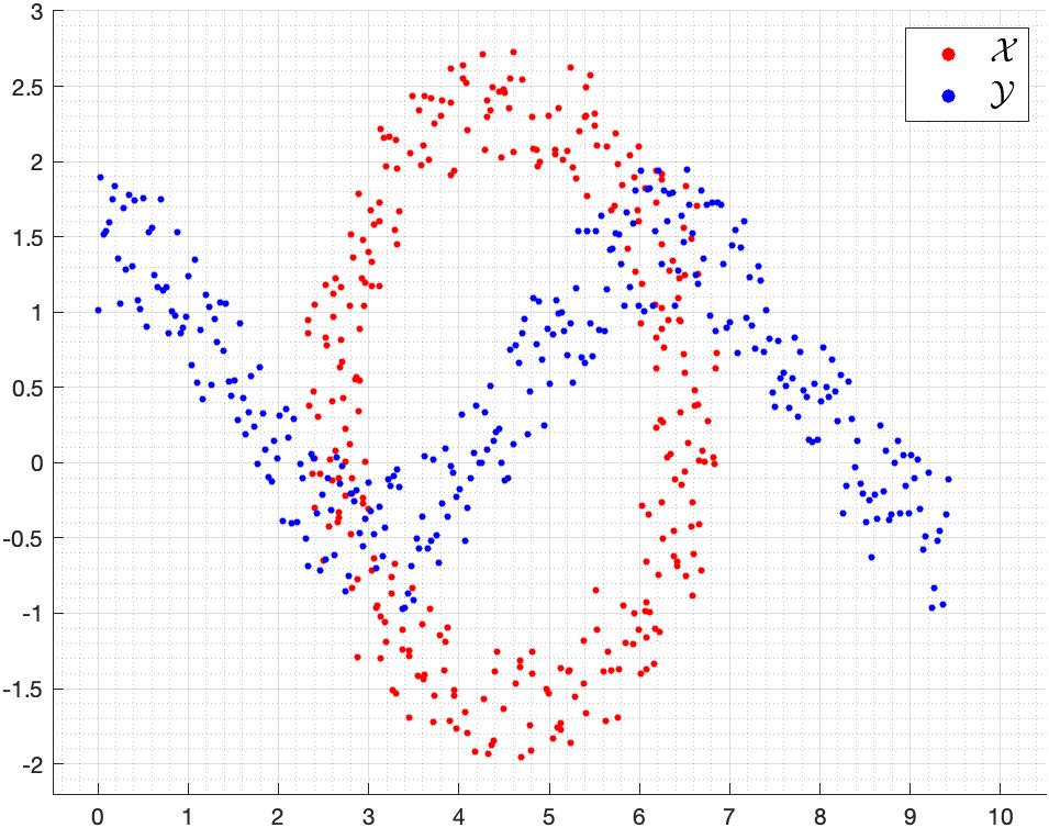
We start by a small dataset of 300 data points in 2-dimensional space, in order to demonstrate how our algorithm works. Figure 1 demonstrates our two discrete distributions: in red and in blue.
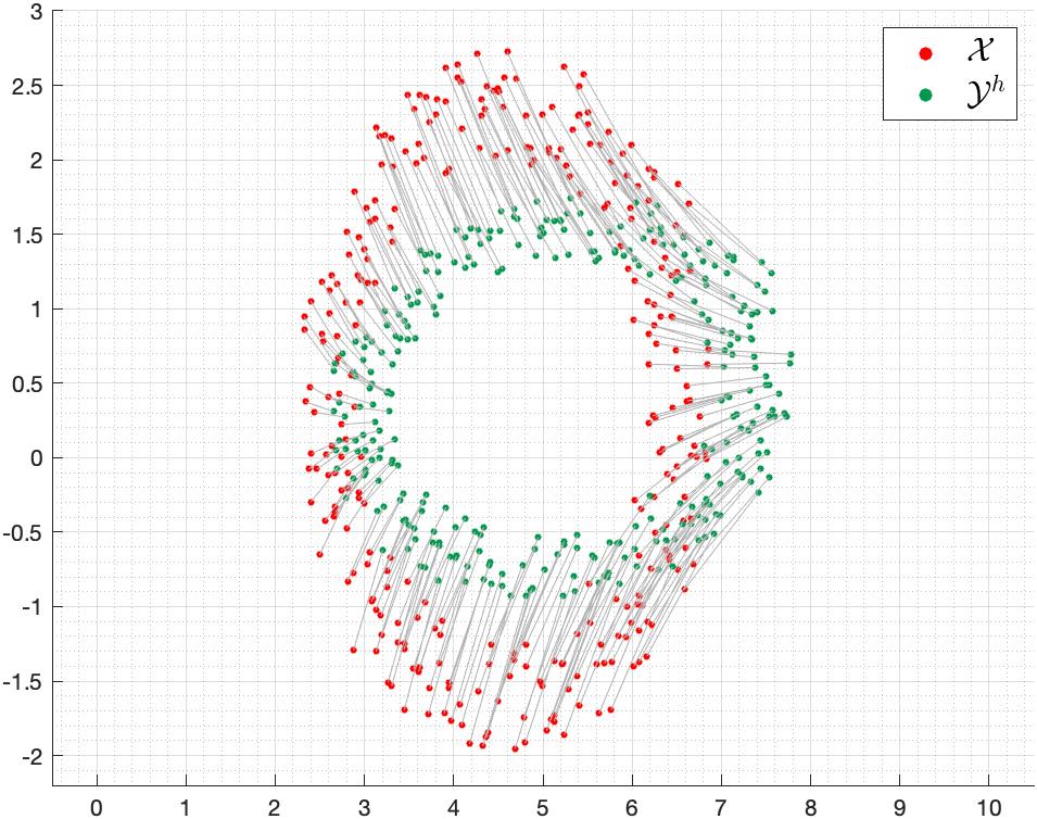
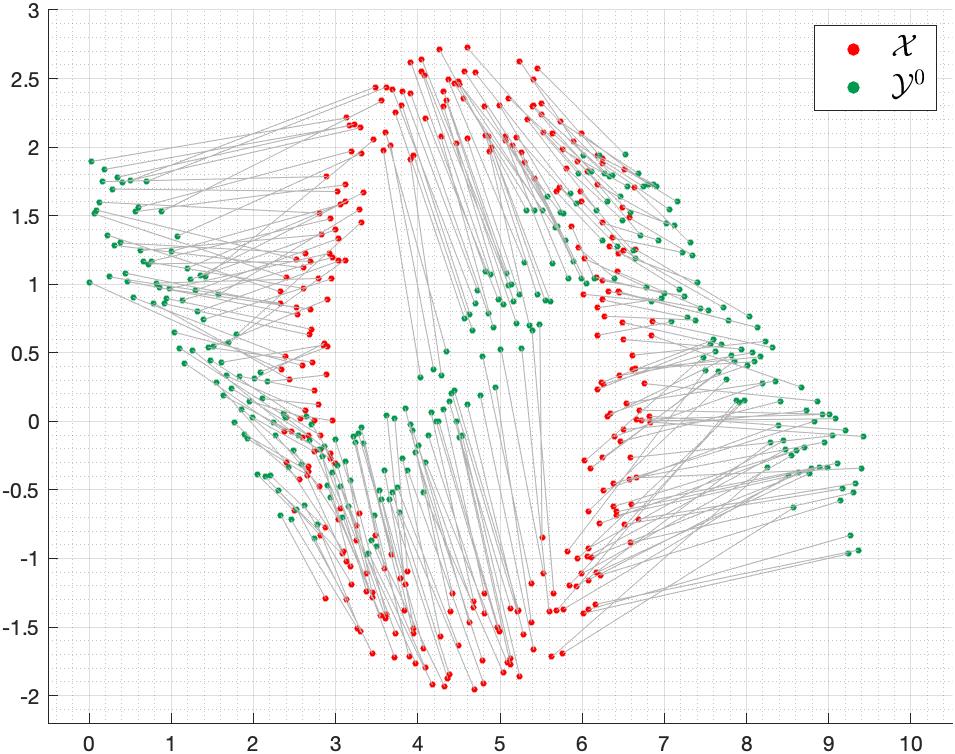
Our algorithm transforms the distribution into which is shown in green in Figure 2. The gray lines in this figure show the optimal matching between the and leading to total transport cost . This can be considered a lower bound on the cost.
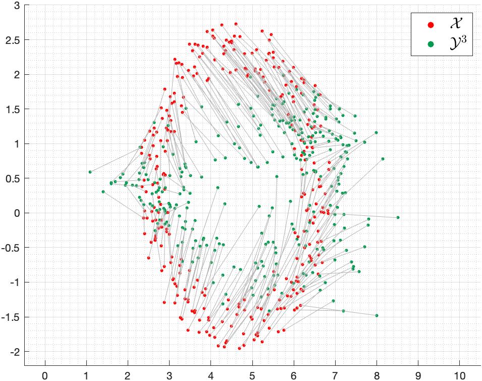
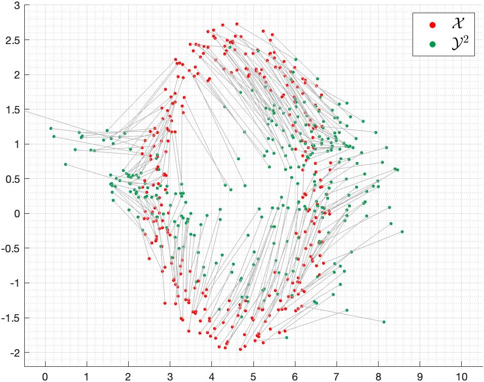
The next step is to gradually transform the back into its original form . We use as the number of steps. Figure LABEL:fig:toy_walkback shows the target distributions () at each of the intermediate states.
fig:toy_walkback
\subfigure[] \subfigure[]
 \subfigure[]
\subfigure[]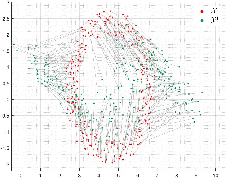 \subfigure[]
| Iteration | ||
|---|---|---|
| 4 | - | 15.47 |
| 3 | 22.01 | 18.06 |
| 2 | 26.10 | 20.86 |
| 1 | 27.65 | 24.50 |
| 0 | 31.23 | 29.06 |
Table 1 shows the results of optimizing the problem along the homotopy path. At each iteration, we update the for the intermediate distribution , using a linear-time algorithm (Duan and Pettie, 2014). Using a more comprehensive algorithm (e.g., algorithm by Duff and Koster (2001) with cubic running time) yields the same results as when we use the linear-time algorithm, because we initiate the homotopy path with an optimal solution, and at each homotopy step, the solution from previous iteration is nearly optimal, so we only have to make small adjustments to it.
The third column in Table 1 shows the total cost corresponding to the combination of and at each step. This basically means using the solution from the previous step for the current step. Clearly, the improvement achieved by at each step is relatively small, because the solution from the previous step is almost optimal and considerably close to the optimal solution for the current step. Note that when we use a random permutation matrix for , the total cost is above 60 on average.
When we apply the cubic running time algorithm by Duff and Koster (2001) directly to and , the optimal solution is the same as the optimal solution obtained by our homotopy algorithm. Also, at each iteration along the homotopy path, the cubic running time algorithm finds the same solution as the linear algorithm. Next, we investigate the effect of homotopy path discretization for this example (i.e., the number of homotopy steps).
Effect of the homotopy path discretization.
To investigate the effect of the number of steps, , we repeat this experiment with and . The results are shown in Tables 2 and 3.
| Iteration | ||
|---|---|---|
| 2 | - | 15.47 |
| 1 | 33.63 | 20.86 |
| 0 | 37.59 | 29.06 |
| Iteration | ||
|---|---|---|
| 8 | - | 15.47 |
| 7 | 17.38 | 16.29 |
| 6 | 19.30 | 18.06 |
| 5 | 21.16 | 19.50 |
| 4 | 22.10 | 20.86 |
| 3 | 23.43 | 22.48 |
| 2 | 25.32 | 24.50 |
| 1 | 27.40 | 26.85 |
| 0 | 29.72 | 29.06 |
Figure 4 demonstrates the total cost associated with the solutions we trace on the homotopy path and how they are affected by the choice of .
The horizontal axis in this Figure corresponds to the homotopy path, normalized between 0 () and 1 (). The vertical axis shows the value of for the solutions we trace along the path.
As an example, let’s walk along the path for the case of , the blue line in Figure 4. We start from 0 (far left of horizontal axis) on the homotopy path where the target distribution is , the optimal solution is , and the total transport cost is . We then compute the intermediate , midway along the homotopy path (i.e., 0.5 on the horizontal axis). This intermediate distribution is basically . The cost of using to transport to is 33.63 (see the blue line at 0.5 on the homotopy path). is optimal to transport to , not to transport to . Next step is to use to optimize the transport plan between and , using as the initial solution. This yields , corresponding to the drop in from 33.63 to 20.86, at point 0.5 on the homotopy path. In the next homotopy iteration, we transform to . Using as the transport plan between and leads to , as the blue line reaches the far right of horizontal axis. Using to improve yields which is the optimal transport plan between and , leading to . The improvement from 37.59 to 29.06 is depicted by the final drop in blue line at the far right of horizontal axis in Figure 4, marking the end of this homotopy path.
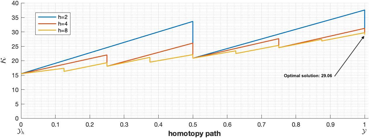
When we make the discretization of the path finer, clearly, the solutions we trace are much closer and as a result, there are less fluctuations along the path. When is increased to , the fluctuations are very small and the cost is changing almost linearly along the path, so we do not see a need to refine the discretization to .
5 Other experiments
We further experiment on a dataset of randomly generated data with and , and observe that our homotopy algorithm is faster than the cubic running time algorithm, while it finds the same optimal solution. This trend repeated when we experiment on MNIST/CIFAR images, in the setting defined by Guo et al. (2020).
6 Conclusion and future work
We presented the outline of a homotopy algorithm for the optimal transport problem with overall complexity of . To complete this work, we need to prove that the updates along the homotopy path have complexity no more than . This seems plausible, because there are algorithms in the literature that can provide updates in near-linear time with some approximation guarantees (Altschuler et al., 2017). We aim to improve this by proving that the updates along the homotopy path can be optimal with no approximation. The best known practical complexity bound for this problem is Guo et al. (2020).
Acknowledgements
R.Y. was supported by a fellowship from the Department of Veteran Affairs. The views expressed in this manuscript are those of the author and do not necessarily reflect the position or policy of the Department of Veterans Affairs or the United States government.
References
- Altschuler et al. (2017) Jason Altschuler, Jonathan Niles-Weed, and Philippe Rigollet. Near-linear time approximation algorithms for optimal transport via Sinkhorn iteration. In Advances in Neural Information Processing Systems, pages 1964–1974, 2017.
- Anandkumar et al. (2017) Anima Anandkumar, Yuan Deng, Rong Ge, and Hossein Mobahi. Homotopy analysis for tensor PCA. In Conference on Learning Theory, pages 79–104, 2017.
- Buttazzo et al. (2012) Giuseppe Buttazzo, Luigi De Pascale, and Paola Gori-Giorgi. Optimal-transport formulation of electronic density-functional theory. Physical Review A, 85(6):062502, 2012.
- Cuturi (2013) Marco Cuturi. Sinkhorn distances: Lightspeed computation of optimal transport. In Advances in Neural Information Processing Systems, pages 2292–2300, 2013.
- Deadman et al. (2012) Edvin Deadman, Nicholas J Higham, and Rui Ralha. Blocked schur algorithms for computing the matrix square root. In International Workshop on Applied Parallel Computing, pages 171–182. Springer, 2012.
- Duan and Pettie (2014) Ran Duan and Seth Pettie. Linear-time approximation for maximum weight matching. Journal of the ACM (JACM), 61(1):1–23, 2014.
- Duff and Koster (2001) Iain S Duff and Jacko Koster. On algorithms for permuting large entries to the diagonal of a sparse matrix. SIAM Journal on Matrix Analysis and Applications, 22(4):973–996, 2001.
- Dunlavy and O’Leary (2005) Daniel M. Dunlavy and Dianne P. O’Leary. Homotopy optimization methods for global optimization. Technical report, Sandia National Laboratories, 2005.
- Galichon (2018) Alfred Galichon. Optimal transport methods in economics. Princeton University Press, 2018.
- Golub and Van Loan (2012) Gene H Golub and Charles F Van Loan. Matrix Computations. JHU Press, Baltimore, 4th edition, 2012.
- Gramfort et al. (2015) Alexandre Gramfort, Gabriel Peyré, and Marco Cuturi. Fast optimal transport averaging of neuroimaging data. In International Conference on Information Processing in Medical Imaging, pages 261–272. Springer, 2015.
- Guo et al. (2020) Wenshuo Guo, Nhat Ho, and Michael Jordan. Fast algorithms for computational optimal transport and wasserstein barycenter. In International Conference on Artificial Intelligence and Statistics, pages 2088–2097, 2020.
- Halko et al. (2011) Nathan Halko, Per-Gunnar Martinsson, and Joel A Tropp. Finding structure with randomness: Probabilistic algorithms for constructing approximate matrix decompositions. SIAM Review, 53(2):217–288, 2011.
- Higham (1987) Nicholas J Higham. Computing real square roots of a real matrix. Linear Algebra and Its Applications, 88:405–430, 1987.
- Higham et al. (2005) Nicholas J Higham, D Steven Mackey, Niloufer Mackey, and Françoise Tisseur. Functions preserving matrix groups and iterations for the matrix square root. SIAM Journal on Matrix Analysis and Applications, 26(3):849–877, 2005.
- Lin et al. (2020a) Tianyi Lin, Nhat Ho, and Michael I Jordan. On efficient optimal transport: An analysis of greedy and accelerated mirror descent algorithms. arXiv preprint arXiv:1901.06482, 2020a.
- Lin et al. (2020b) Tianyi Lin, Zeyu Zheng, Elynn Y Chen, Marco Cuturi, and Michael I Jordan. On projection robust optimal transport: Sample complexity and model misspecification. arXiv preprint arXiv:2006.12301, 2020b.
- Mobahi and Fisher III (2015) Hossein Mobahi and John W. Fisher III. On the link between Gaussian homotopy continuation and convex envelopes. In Lecture Notes in Computer Science (EMMCVPR), pages 43–56. Springer, 2015.
- Nocedal and Wright (2006) Jorge Nocedal and Stephen Wright. Numerical Optimization. Springer, New York, 2nd edition, 2006. ISBN 9780387400655.
- Pele and Werman (2009) Ofir Pele and Michael Werman. Fast and robust earth mover’s distances. In IEEE 12th International Conference on Computer Vision, pages 460–467. IEEE, 2009.
- Peyré et al. (2019) Gabriel Peyré, Marco Cuturi, et al. Computational optimal transport: With applications to data science. Foundations and Trends® in Machine Learning, 11(5-6):355–607, 2019.
- Schiebinger et al. (2019) Geoffrey Schiebinger, Jian Shu, Marcin Tabaka, Brian Cleary, Vidya Subramanian, Aryeh Solomon, Joshua Gould, Siyan Liu, Stacie Lin, Peter Berube, et al. Optimal-transport analysis of single-cell gene expression identifies developmental trajectories in reprogramming. Cell, 176(4):928–943, 2019.
- Villani (2008) Cédric Villani. Optimal transport: old and new, volume 338. Springer Science & Business Media, 2008.
- Yousefzadeh and O’Leary (2020) Roozbeh Yousefzadeh and Dianne P. O’Leary. Deep learning interpretation: Flip points and homotopy methods. In Proceedings of Machine Learning Research, volume 107, pages 1–26, 2020.