Three-dimensional $O(N)$-invariant $\phi^{4}$ models at criticality for $N\geq 4$

Abstract

We study the $O(N)$-invariant $\phi^{4}$ model on the simple cubic lattice by using Monte Carlo simulations. By using a finite size scaling analysis, we obtain accurate estimates for the critical exponents $\nu$ and $\eta$ for $N=4$, $5$, $6$, $8$, $10$, and $12$. We study the model for each $N$ for at least three different values of the parameter $\lambda$ to control leading corrections to scaling. We compare our results with those obtained by other theoretical methods.

I Introduction

We study the $\phi^{4}$ model on the simple cubic lattice by using Monte Carlo (MC) simulations combined with a finite size scaling (FSS) Barber analysis. The $\phi^{4}$ model is a prototypical model to investigate critical phenomena. The reduced Hamiltonian of the $N$-component $\phi^{4}$ model, for a vanishing external field, is given by

$${\cal H}=-\beta\sum_{<x,y>}\vec{\phi}_{x}\cdot\vec{\phi}_{y}+\sum_{x}\left[\vec{\phi}_{x}^{\;2}+\lambda(\vec{\phi}_{x}^{\;2}-1)^{2}\right]\;,$$ (1)

where $\vec{\phi}_{x}$ is a vector with $N$ real components. We label the sites of the simple cubic lattice by $x=(x_{0},x_{1},x_{2})$, where $x_{i}\in\{1,2,\ldots,L_{i}\}$. Furthermore, $<xy>$ denotes a pair of nearest neighbors on the lattice. For $\lambda=0$ we get the Gaussian model or free field theory on the lattice. For $\lambda>0$, the model undergoes a second order phase transition. In the limit $\lambda\rightarrow\infty$ the field is forced to unit length $|\vec{\phi}_{x}|=1$. In the literature, the model in this limit is referred to as $O(N)$ vector model. In the following we shall use the notation $\lambda=\infty$ to refer to this limit.

The modern theory of critical phenomena is the renormalization group (RG), going back to the seventies of the last century. The RG-theory furnishes a general framework but also provides computational tools like the $\epsilon$-expansion or the functional renormalization group (FRG) method.

In the neighborhood of the critical temperature, at a second order phase transition, thermodynamic quantities diverge, following power laws. For example, the correlation length $\xi$ in the thermodynamic limit, behaves as

$$\xi=at^{-\nu}\;\left(1+bt^{\theta}+ct+...\right)\;,$$ (2)

where $t=(T-T_{c})/T_{c}$ is the reduced temperature and $\nu$ the critical exponent of the correlation length. The power law is subject to confluent and analytic corrections. In eq. (2) we give the leading ones. The correction exponent can be written as $\theta=\nu\omega$, where $\omega$ naturally appears in FSS.

The RG predicts that second order phase transitions fall into universality classes. For a given class, critical exponents such as $\nu$ and correction exponents such as $\omega$ assume unique values. The same holds for so called amplitude ratios. A universality class is characterized by a few qualitative features of the system. These are the spatial dimension, the symmetry properties of the order parameter and the range of the interaction. Accurate experiments and theoretical calculations support the universality hypothesis. In the case of the model discussed here, the universality class, for a given value of $N$, should not depend on the parameter $0<\lambda\leq\infty$. For reviews on critical phenomena and the RG see, for example WiKo ; Fisher74 ; Fisher98 ; Kleinert ; PeVi02 .

Great progress has been achieved recently by using the so called conformal bootstrap (CB) method. In particular in the case of the three-dimensional Ising universality class, corresponding to $N=1$, the accuracy that has been reached for critical exponents clearly surpasses that of other theoretical methods. See refs. Kos:2016ysd ; Simmons-Duffin:2016wlq and references therein. Very recently also highly accurate estimates che19 were obtained for the XY universality class, $N=2$, surpassing the accuracy of results obtained by lattice methods. In the case of the Heisenberg universality class, $N=3$, accurate results were provided in che20 . Results for $N=4$ are given in refs. Kos15 ; CaHaSe16 . For a review on the CB method, see for example revCB .

In the last few years, progress has also been achieved by using other methods. The $\epsilon$-expansion for critical exponents of $O(N)$-invariant models has been extended to 6-loops KoPa17 and to 7-loops Sch18 . An analysis of the 7-loop series is provided, for example, in refs. Sha21 ; AbSa21 . In ref. DePo20 accurate results were obtained for critical exponents and the correction exponent $\omega$ for three-dimensional $O(N)$-invariant systems by using the FRG method. For a recent review on the FRG method see ref. Eich21 . These two approaches can be applied to a wide range of problems. For example, both the $\epsilon$-expansion as well as the FRG method can be applied to dynamic problems.

The Monte Carlo simulation of lattice models in combination with a FSS analysis is well established in the study of critical phenomena and might serve as benchmark of these methods. Recently in refs. Landau18 ; myIso ; Xu19 ; myClock ; myIco accurate estimates of the critical exponents for $N=1$, $2$, and $3$ were obtained. For references to the bulk of previous work see refs. Landau18 ; myIso ; Xu19 ; myClock ; myIco and the review PeVi02 . Here we like to bridge the gap to the $1/N$ expansion. To this end we study the $\phi^{4}$ model for $N=4$, $5$, $6$, $8$, $10$, and $12$. Previous simulations for these values of $N$ are discussed in the conclusions. For a review on the large $N$-expansion see, for example MoZi03 . For a physical motivation to study the $\phi^{4}$ model for $N=4$ and $5$, see for example sections 6.1 and 6.2 of the review PeVi02 .

The outline of the paper is the following. In section II, we define the observables that we measure. In section III we discuss corrections to scaling. In the main part of the paper, we discuss our simulations and the analysis of the data. In section IV we briefly sketch the Monte Carlo algorithm and its implementation. In sections V and VI we discuss the cases $N=4$ and $5$, respectively. The simulations and the analysis of the data for $N\geq 6$ are briefly sketched in section VII. Finally, in section VIII we conclude and compare our results for the critical exponents with those obtained by various methods given in the literature.

II The observables

Here we study the same observables as in previous work, see for example section II B of ref. myClock . For completeness we recall the definitions of the quantities that we have measured.

In our study, the linear lattice size $L=L_{0}=L_{1}=L_{2}$ is equal in all three directions throughout. We employ periodic boundary conditions.

The energy of a given spin configuration is defined as

$$E=\sum_{<xy>}\vec{\phi}_{x}\cdot\vec{\phi}_{y}\;\;.$$ (3)

The magnetic susceptibility $\chi$ and the second moment correlation length $\xi_{2nd}$ are defined as

$$\chi\equiv\frac{1}{V}\left\langle\Big{(}\sum_{x}\vec{\phi}_{x}\Big{)}^{2}\right\rangle\;\;,$$ (4)

where $V=L^{3}$ and

$$\xi_{2nd}\equiv\sqrt{\frac{\chi/F-1}{4\sin^{2}\pi/L}}\;\;,$$ (5)

where

$$F\equiv\frac{1}{V}\left\langle\Big{|}\sum_{x}\exp\left(i\frac{2\pi x_{k}}{L}\right)\vec{\phi}_{x}\Big{|}^{2}\right\rangle$$ (6)

is the Fourier transform of the correlation function at the lowest non-zero momentum. In our simulations, we have measured $F$ for the three directions $k=0,1,2$ and have averaged these three results.

In addition to elementary quantities like the energy, the magnetization, the specific heat or the magnetic susceptibility, we compute a number of so-called phenomenological couplings, that means quantities that, in the critical limit, are invariant under RG transformations. We consider the Binder parameter $U_{4}$ and its sixth-order generalization $U_{6}$, defined as

$$U_{2j}\equiv\frac{\langle\vec{m}^{2j}\rangle}{\langle\vec{m}^{2}\rangle^{j}},$$ (7)

where $\vec{m}=\frac{1}{V}\,\sum_{x}\vec{\phi}_{x}$ is the magnetization of a given spin configuration. We also consider the ratio $R_{Z}\equiv Z_{a}/Z_{p}$ of the partition function $Z_{a}$ of a system with anti-periodic boundary conditions in one of the three directions and the partition function $Z_{p}$ of a system with periodic boundary conditions in all directions. This quantity is computed by using the cluster algorithm. For a discussion see Appendix A 2 of ref. XY1 . In the following we shall refer to the RG-invariant quantities $U_{2j}$, $Z_{a}/Z_{p}$ and $\xi_{2nd}/L$ using the symbol $R$.

In our analysis we need the observables as a function of $\beta$ in some neighborhood of the simulation point. To this end we have computed the coefficients of the Taylor expansion of the observables up to the third order. For example the first derivative of the expectation value $\langle A\rangle$ of an observable $A$ is given by

$$\frac{\partial\langle A\rangle}{\partial\beta}=\langle AE\rangle-\langle A\rangle\langle E\rangle\;\;.$$ (8)

III Corrections to scaling

In the analysis of the data corrections to scaling play an important role. Systematic errors are caused by corrections that are not or not exactly taken into account in the Ansätze that are used to fit the data.

Based on the general framework of the RG-theory we expect that the quantities that we are dealing with in the FSS analysis behave at the critical point as

$$A(L)=aL^{x}(1+\sum_{i}b_{i}L^{-\omega_{i}}+\sum_{ij}c_{ij}L^{-\omega_{i}-\omega_{j}}+...)\;,$$ (9)

where $x$ is the critical exponent we like to determine and $\omega_{i}>0$ are correction exponents. RG-theory predicts that $x$ and $\omega_{i}$ are universal, while $a$, $b_{i}$ and $c_{ij}$ depend on the particular system that is considered. In the case of the model studied here, these coefficients are functions of the parameter $\lambda$.

In practice only a small number of correction terms can be taken into account, since the statistical error of the estimates obtained by the fit rapidly increases with the number of free parameters. The systematic error can be reduced by going to larger lattice sizes $L$. However we are limited in this direction, since the CPU time that is required to keep the statistical error constant essentially grows as $L^{d+z}$, where $d$ is the dimension of the system and the dynamical critical exponent $z>0$ for the algorithms used here. In order to decide on the design of the study, information on the corrections is needed. Getting information by using FSS studies, in practice one is restricted to the leading correction. In the case of subleading corrections we have to rely on other theoretical methods.

Various methods give consistently $\omega\approx 0.8$ for the exponent of the leading correction to scaling for $N\lessapprox 12$. Since the amplitudes of corrections $b_{i}$ depend on the details of the system, in our case, one might try to find a value $\lambda^{*}$ such that the amplitude of the leading correction vanishes: $b(\lambda^{*})=0$. RG-theory tells us that $\lambda^{*}$ is the same for different quantities. Models with a vanishing amplitude of the leading correction to scaling are denoted as improved models. This idea had been exploited first by using high temperature series expansions of such models ChFiNi ; FiCh . For early Monte Carlo simulations of improved models sharing the universality class of the three-dimensional Ising model see for example refs. Bloete ; Ballesteros ; KlausStefano . In CaPe99 it has been pointed out that for the $\phi^{4}$ model on the simple cubic lattice in the large $N$ limit $\lambda^{*}$ does not exist. For $N=1$, $2$, $3$, and $4$ a finite $\lambda^{*}$ has been found. Most recent estimates are $\lambda^{*}\approx 1.1$ myPhi4 for $N=1$, $\lambda^{*}=2.15(5)$ XY2 for $N=2$, $\lambda^{*}=5.17(11)$ myIco for $N=3$ and $\lambda^{*}=20_{-6}^{+15}$ O234 for $N=4$. The value of $\lambda^{*}$ is rapidly increasing with $N$. In the case of $N=5$ it is not fully settled, whether $\lambda^{*}$ exist. If yes, it is close to the limiting case $\lambda=\infty$ ourO5 . Analyzing our data, we confirm that $\lambda^{*}$ for $N=4$ exists, while for $N=5$ this is highly unlikely. The result that for $N>5$ no $\lambda^{*}$ exists is very robust. As a consequence, the outline of the study for $N=4$ is very similar to our recent work myClock ; myIco , where we studied models in the XY and Heisenberg universality classes. For larger values of $N$ we focus on improved observables, which are constructed such that leading corrections are suppressed for any model. Still the accuracy of the estimates of critical exponents is lower for larger values of $N$ than for $N=4$.

III.1 Subleading corrections

In the analysis of our data, we use prior information on subleading corrections to scaling. In section III A of ref. myClock we argue, based on the literature, that there should be only a small dependence of the irrelevant RG-eigenvalues on $N$. Therefore the discussion of section III A of ref. myClock should apply to the present case $4\leq N\leq 12$ at least on a qualitative level.

The most important subleading correction should be due to the breaking of the rotational symmetry by the simple cubic lattice. Corrections related with the spatial anisotropy are discussed in ref. ROT98 . To this end, the two-point function of $O(N)$-invariant models is studied by using the $1/N$-expansion, field-theoretic methods and the high temperature series expansion. Results for $\sigma$, for various values of $N$, are summarized in table VI (table VIII of the preprint version), where the correction exponent is $\omega_{NR}=2+\sigma$. In the large $N$-limit one obtains ROT98

$$\sigma=\frac{32}{21\pi^{2}N}+O\left(N^{-2}\right)\;.$$ (10)

According to the authors, this expression gives a reasonable numerical value at best down to $N=8$. Looking at table VI of ref. ROT98 , it seems plausible that $\sigma$ has a plateau-like maximum at $N=3$ up to $4$ and then slowly decreases. This behavior is supported both by the high temperature series expansion as well as the field-theoretic methods.

We might gauge the estimates of ref. ROT98 by using the highly accurate result $\sigma=0.022665(28)$ obtained by using the CB method in ref. Simmons-Duffin:2016wlq for $N=1$. This suggests in particular that for the values of $N$ studied here, the field theoretic estimates of $\sigma$ given in ref. ROT98 are too small.

Based on these considerations, we use the numerical value

$$\sigma=\mbox{min}\left[0.023,\frac{32}{21\pi^{2}N}\right]$$ (11)

with an error of $0.005$ in the analysis of our data. We checked that the estimates of the quantities we are interested in change only by little, when $\sigma$ is varied within this error band.

In addition, there are corrections that are intrinsic to the quantity that is studied. For example in the case of the magnetic susceptibility there is the analytic background. This can be interpreted as a correction with the exponent $2-\eta$. It should also appear in the Binder cumulant $U_{4}$ that contains $\langle m^{2}\rangle$ in its definition. In the case of $\xi_{2nd}/L$ there is, by construction, a correction with the exponent $2$.

IV The Monte Carlo algorithm and its implementation

We simulated by using a hybrid of local updates and the wall cluster algorithm KlausStefano . The probability to delete the link between the nearest neighbor sites $x$ and $y$ is the same as for the Swendsen-Wang (SW) SW or the single cluster algorithm Wolff . It differs in the choice of the clusters to be flipped. In the case of the SW algorithm, all clusters are constructed, and a cluster is flipped with probability $1/2$. In the case of the single cluster algorithm, a single site of the lattice is randomly chosen. The cluster that contains this site is flipped. To this end, only this cluster has to be constructed. In the case of the wall cluster algorithm, a plain of the lattice is randomly selected. All clusters that share a site with this plain are flipped. Also here, only these clusters need to be constructed. In order to determine $Z_{a}/Z_{p}$, we have to go through all $N$ components of the field XY1 .

We have implemented overrelaxation updates

$$\vec{\phi}_{x}^{\;\;{}^{\prime}}=2\frac{\vec{\Phi}_{x}\cdot\vec{\phi}_{x}}{\vec{\Phi}_{x}^{2}}\vec{\Phi}_{x}-\vec{\phi}_{x}\;\;,$$ (12)

where

$$\vec{\Phi}_{x}=\sum_{y.nn.x}\vec{\phi}_{y}\;\;,$$ (13)

where $\sum_{y.nn.x}$ is the sum over all nearest neighbors $y$ of the site $x$. Note that these updates do not change the value of the Hamiltonian and therefore no accept/reject step is needed. It is computationally quite cheap, since no random number and no evaluation of $\exp()$ is needed. In the case of the overrelaxation update we run through the lattice in typewriter fashion. As the cluster update, the overrelaxation update does not change $|\vec{\phi}_{x}|$.

For finite $\lambda$, we perform Metropolis updates to change $|\vec{\phi}_{x}|$. For each site, we perform two subsequent updates. We use the acceptance probability

$$P_{acc}=\mbox{min}\left[1,\exp(-H(\phi^{\prime})+H(\phi))\right]\;.$$ (14)

For the first hit, we generate the proposal by

$$\phi_{x,i}^{\prime}=\phi_{x,i}+s_{1}(r-0.5)$$ (15)

for each component $i$ of the field at the site $x$. $r$ is a uniformly distributed random number in $[0,1)$ and the step size $s_{1}$ is tuned such that the acceptance rate is roughly $50\%$. In the case of the second hit, we randomly select a single component $j$. Now $\phi_{x,j}^{\prime}=\phi_{x,j}+s_{2}(r-0.5)$, while all other components keep their value. Also here, we tune $s_{2}$ such that the acceptance rate is roughly $50\%$. Also here, we run through the lattice in typewriter fashion.

In the limit $\lambda=\infty$, we simulated the model by using a hybrid of the overrelaxation algorithm and the wall cluster algorithm KlausStefano . Below we give the update sequence used for $\lambda=\infty$ and $N=5$, $6$, $8$, $10$, and $12$ as C-code:
ROTATE; over(); over(); for(ic=0;ic<N;ic++) wall_0(ic); measure();
ROTATE; over(); over(); for(ic=0;ic<N;ic++) wall_1(ic); measure();
ROTATE; over(); over(); for(ic=0;ic<N;ic++) wall_2(ic); measure();

Here over() is a full sweep with the overrelaxation update over the lattice. wall_k(ic) is a wall-cluster update with a plain perpendicular to the k-axis. The component ic of the field is updated. The position of the plain on the k-axis is randomly chosen for each component of the field. Note that in the cluster and Metropolis updates the axis play a special role. This does not invalidate the updates but might lead to a certain degradation of the performance. Therefore we interleave the updates with global rotations of the field. The rotations ROTATE are build from a sequence of rotations by a random angle between two axis. For $\lambda=\infty$ the condition $|\vec{\phi}_{x}^{\;2}|=1$ might be lost due to rounding errors. Therefore we normalize the field $\vec{\phi}_{x}$ after each update cycle. For finite $\lambda$, we have added a sweep with the local two hit Metropolis update following ROTATE.

In the case of $N=4$ the update cycle for $\lambda=\infty$ is given by
ROTATE; over(); for(ic=0;ic<N;ic++) wall_0(ic); measure();
over(); for(ic=0;ic<N;ic++) wall_1(ic); measure();
over(); for(ic=0;ic<N;ic++) wall_2(ic); measure();

Again, for finite $\lambda$ a sweep using the Metropolis algorithm is added for each measurement.

Note that the composition of the update cycles is not tuned. Essentially it is based on an ad hoc decision guided by the experience gained in previous work.

For a certain fraction of the simulations for $N=4$ we have used the SIMD-oriented Fast Mersenne Twister (SMFT) twister pseudo-random number generator, where SIMD is the abbreviation for single instruction, multiple data. In the remaining part of the simulations for $N=4$ and for larger values of $N$ we have used a hybrid of generators, where one component is the xoshiro256+ taken from VignaWWW . For a discussion of the generator see ViBl18 . As second component we used a 96 bit linear congruential generator with the multiplier and the increment $a=c=$0xc580cadd754f7336d2eaa27d and the modulus $m=2^{96}$ suggested by O’Neill ONeill_minimal . In this case we used our own implementation. The third component is a multiply-with-carry generator taken from KISS_wiki . For a more detailed discussion see the Appendix A of ref. myIso .

Throughout this work, least square fits were performed by using the function curve_fit() contained in the SciPy library pythonSciPy . Plots were generated by using the Matplotlib library plotting .

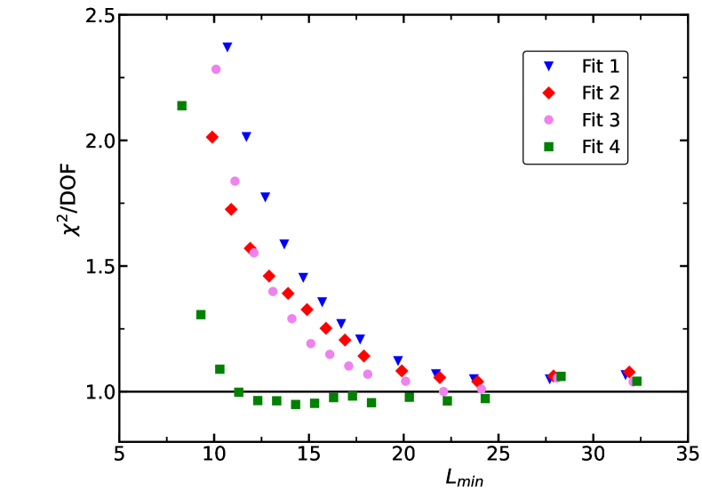
Fitting our data, we take lattice sizes $L\geq L_{min}$ into account. For small values of $L_{min}$, $\chi^{2}/$DOF decreases with increasing $L_{min}$, since the magnitudes of corrections that are not taken into account in the Ansatz decrease with increasing lattice size $L$. At some point $\chi^{2}/$DOF levels off, since the magnitudes of these corrections become smaller than the statistical error. On the other hand, with increasing $L_{min}$, the statistical error of the estimates of fit parameters is increasing. Often in the literature, the estimates of fit parameters obtained for the smallest $L_{min}$ with an acceptable goodness of the fit are taken as the final results.

Here, in order to get a better handle on systematic errors due to corrections that are not included in the Ansatz, the final results are chosen such that they are compatible with estimates obtained by using several different Ansätze, containing more or less correction terms. For a more comprehensive discussion of this issue see section V of ref. myIco .

V The simulations and the analysis of the data for $N=4$

We simulated at $\lambda=2$, $4$, $12.5$, $18.5$, $20$, and $\infty$. Let us briefly summarize the lattice sizes and the statistics of the simulations. Note that some of the simulations were already performed a few years ago, leading to different choices of the lattice sizes for different values of $\lambda$. Most of the simulations were performed on desktop PCs at the institute of theoretical physics of the university of Heidelberg. The CPU times quoted below refer to the time that would be needed on a single core of an AMD EPYC^TM 7351P CPU. For example, on a single core of an Intel(R) Xeon(R) CPU E3-1225 v3 the performance of our code is very similar.

For $\lambda=\infty$ we simulated the linear lattice sizes $L=6$, $7$, $8$, …, $20$, $22$, $24$, …, $32$, $36$, $40$, $44$, $48$, $56$, $64$, $72$, $80$, and $200$. Up to $L=20$ we performed $3\times 10^{9}$ measurements. For $L=22$, $24$, $26$, and $28$ we performed $6.2\times 10^{9}$, $5.8\times 10^{9}$, $3.8\times 10^{9}$, and $4.6\times 10^{9}$ measurements, respectively. Then the number of measurements monotonically decreases to $4.8\times 10^{8}$ for $L=80$. For $L=200$ only $7.5\times 10^{6}$ measurements were performed. In total these simulations took about 8.5 years of CPU time.

For $\lambda=20$ we simulated the linear lattice sizes $L=6$, $7$, $8$, …, $20$, $22$, $24$, $26$, $30$, $34$, $40$, $50$, $60$, $80$, $100$, $140$, $200$, and $300$. Up to $L=30$ we performed $3\times 10^{9}$ measurements. For larger linear lattice sizes $L$, the number of measurements decreases with increasing $L$. For example for $L=200$ and $300$, we performed $9\times 10^{7}$ and $3\times 10^{7}$, respectively. In total these simulations took about 20.6 years of CPU time.

For $\lambda=18.5$ we simulated the linear lattice sizes $L=8$, $9$, $10$, …, $22$, $24$, $26$, …, $32$, $36$, $40$, $44$, $48$, $56$, $64$, …, $80$, $100$, $120$, and $200$. For $L=10$, we performed $5.4\times 10^{9}$ measurements. This number slowly drops to $2.8\times 10^{9}$ for $L=36$. Then the number of measurements decreases more rapidly with $L$. For example for $L=80$, $100$, $120$, and $200$, we performed $5.9\times 10^{8}$, $2.1\times 10^{8}$, $2.5\times 10^{8}$, and $5.3\times 10^{7}$ measurements, respectively. In total these simulations took about 19.5 years of CPU time.

For $\lambda=12.5$ we simulated the linear lattice sizes $L=6$, $7$, $8$, …, $20$, $24$, $28$, …, $40$, $48$, $56$, $60$, $64$, and $80$. Up to $L=28$ we performed $3\times 10^{9}$ measurements. For example for $L=64$ and $80$, we performed $4.6\times 10^{8}$ and $1.7\times 10^{8}$ measurements, respectively. In total these simulations took about 7.5 years of CPU time.

For $\lambda=4$ we simulated the linear lattice sizes $L=6$, $7$, $8$, …, $22$, $24$, $26$, $28$, $32$, $36$, …, $52$, $60$, $70$, $80$. Up to $L=21$ we performed at least $2.4\times 10^{9}$ measurements. Then the number of measurements decreases with increasing $L$. For example, for $L=70$ and $80$, we performed $4.8\times 10^{8}$ and $1.8\times 10^{8}$ measurements, respectively. In total these simulations took about 6 years of CPU time.

For $\lambda=2$ we simulated the linear lattice sizes $L=6$, $7$, $8$, …, $22$, $24$, $26$, $28$, $32$, $36$, …, $48$, $60$, $80$. The number of measurements for each lattice size is similar to that for $\lambda=4$. In total these simulations took about 4.3 years of CPU time.

Throughout, while the number of measurements decreases with increasing $L$, the CPU time used for a given lattice size $L$, increases with increasing $L$. The same holds for larger values of $N$, discussed below.

V.1 The dimensionless quantities

First we analyzed the behavior of dimensionless quantities. We performed joint fits of all four quantities, $Z_{a}/Z_{p}$, $\xi_{2nd}/L$, $U_{4}$, and $U_{6}$, for two sets of $\lambda$-values. The first set contains $\lambda=4.0$, $12.5$, $18.5$, $20$ and $\infty$, while in the second we consider $\lambda=2.0$, in addition. We use Ansätze of the form

$$R_{i}(\beta_{c},\lambda,L)=R_{i}^{*}+\sum_{k=1}^{k_{max}}c_{i,k}[b(\lambda)a_{i}L^{-\omega}]^{k}+\sum_{j}e_{i,j}(\lambda)L^{-\epsilon_{j}}\;,$$ (16)

where $c_{i,1}=1$ and $b(\lambda)$ is normalized such that $a_{Z_{a}/Z_{p}}=1$. In our fits, we consider $\omega$ as free parameter, while we fix the exponents of subleading corrections. In particular we take $\epsilon_{1}=2-\eta$, where we took the preliminary estimate $\eta=0.03625$, which is close to our final estimate, eq. (30), $\epsilon_{2}=2$, and $\epsilon_{3}=\omega_{NR}=2.023$, eq. (11). The correction with the exponent $\epsilon_{1}$ applies to $U_{4}$, $U_{6}$ and $\xi_{2nd}/L$, the correction with $\epsilon_{2}$ to $\xi_{2nd}/L$, while the correction with the exponent $\omega_{NR}$ is non-vanishing in all four cases. The amplitude of the leading correction $b(\lambda)$ is taken as free parameter for each value of $\lambda$. In principle the $e_{i,j}$ depend on $\lambda$. In order to keep the fits tractable, we used a parameterization to reduce the number of free parameters. In the case of $e_{i,1}$, we used

$$e_{i,1}=d_{i}\;,$$ (17)

$$e_{i,1}=d_{i}+s_{i}\lambda^{-1}$$ (18)

or

$$e_{i,1}=d_{i}+s_{i}\lambda^{-1}+t_{i}\lambda^{-2}\;,$$ (19)

where $d_{i}$, $s_{i}$ and $t_{i}$ are the free parameters of the fit. In our fits, $e_{i,2}$ and $e_{i,3}$ are assumed to be constant. For $e_{i,3}$ this should indeed be a good approximation. In the case of the Ising universality class, for the Blume Capel model on the simple cubic lattice, in ref. myIso , we found that the amplitude of deviations from the rotational invariance depends very little on the parameter $D$, where $D$ plays a similar role as the parameter $\lambda$ of the model studied here.

In our analysis of the data set 1, i.e. for $\lambda=4.0$, $12.5$, $18.5$, $20$ and $\infty$, we consider the following choices, based on the Ansatz (16):

• Fit 1: $k_{max}=1$, parameterization (17)

• Fit 2: $k_{max}=1$, parameterization (18)

• Fit 3: $k_{max}=2$, parameterization (17)

• Fit 4: $k_{max}=2$, parameterization (18)

In Fig. 1 we give the $\chi^{2}/$DOF obtained in these fits as a function of the minimal lattice size $L_{min}$ that is taken into account. In the case of fit 1, we get $\chi^{2}/$DOF $=1.07$ corresponding to $p=0.20$ at $L_{min}=22$. In the case of fit 2 and fit 3, $\chi^{2}/$DOF $\approx 1$ is reached for somewhat smaller $L_{min}$. For fit 4, we get $\chi^{2}/$DOF $=1.00$ already for $L_{min}=11$. We checked that using the parameterization (19) or adding a term proportional to $L^{-3\omega}$ improves the goodness of the fits only by little. Finally, we performed fits with an additional correction term on top of fit 4, where the correction exponent is a free parameter. Here we get $\chi^{2}/$DOF $=1.06$ and $\chi^{2}/$DOF $=0.97$ already for $L_{min}=7$ and $8$, respectively. We get $\omega^{\prime}=4.91(24)$ and $4.88(47)$, for $L_{min}=7$ and $8$, respectively. Going to larger $L_{min}$, the statistical error of $\omega^{\prime}$ rapidly increases. The amplitude of this correction is comparatively large. Since $\omega^{\prime}$ is large, this correction plays virtually no role for $L\gtrapprox 10$. One should note that this finding does not mean that there is no correction with $2<\omega^{\prime}<4.9$. Such corrections might just have a small amplitude compared with the $\omega^{\prime}\approx 4.9$ correction.

In a second set of fits we have analyzed in addition the data for $\lambda=2.0$. Still fit 4 gives $\chi^{2}/$DOF $=1.07$ corresponding to $p=0.14$ for $L_{min}=11$ and $\chi^{2}/$DOF $=1.02$ corresponding to $p=0.39$ for $L_{min}=12$. Using the parameterization (19) or adding a term proportional to $L^{-3\omega}$ improves the goodness of the fits only by little.

Figure 1: Joint fits of dimensionless quantities for $\lambda=4.0$, $12.5$, $18.5$, $20$, and $\infty$ for $N=4$. Numerical estimates for $\chi^{2}/$DOF obtained from the fits 1, 2, 3, and 4, which are discussed in the text, are plotted versus the minimal lattice size $L_{min}$ that is taken into account. Note that the values on the $x$-axis are slightly shifted to reduce overlap of the symbols.

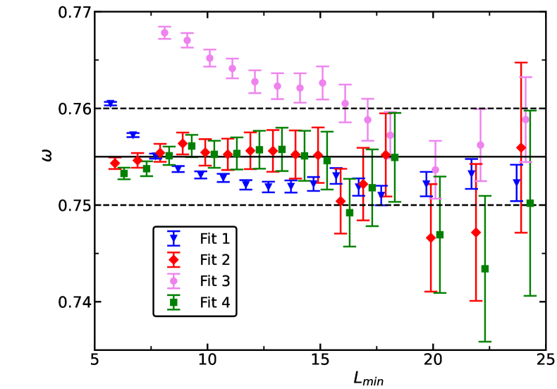
In Fig. 2 we give our results for the correction exponent $\omega$ obtained by using the fits 1, 2, 3, and 4 with the data for $\lambda=2$, $4$, $12.5$, $18.5$, $20$ and $\infty$. Here we give all estimates, irrespective of the $\chi^{2}/$DOF. As our final result we consider

$$\omega=0.755(5)\;.$$ (20)

It is chosen such that it contains the results obtained by using the fits 2 and 4 up to $L_{min}=15$, while the results of fit 3 are contained for $L_{min}=18$, $20$, and $22$. The results for fit 1 are contained from $L_{min}=7$ up to $28$. Here and in the following we mean by “the fit is contained” that the central estimate obtained by the fit $\pm$ its error lies within the interval given by our final result $\pm$ our final error estimate. To get an idea on the amplitude of corrections to scaling we quote the results for fit 4 and $L_{min}=12$: $b=0.00474(11)$, $0.00038(11)$, $0.00003(11)$, $-0.00217(11)$, $-0.01495(15)$, and $-0.02868(22)$ for $\lambda=\infty$, $20$, $18.5$, $12.5$, $4.0$, and $2.0$, respectively. Taking into account also the results of other fits, linearly interpolating $b(\lambda)$ for $\lambda=18.5$ and $20$ we determine the zero of $b(\lambda)$ as

$$\lambda^{*}=18.4(9)\;,$$ (21)

which can be compared with the previous estimate $\lambda^{*}=20_{-6}^{+15}$ O234 .

Figure 2: Numerical estimates of the correction exponent $\omega$ for $N=4$ obtained from joint fits of the data for $\lambda=2$, $4$, $12.5$, $18.5$, $20$, and $\infty$ versus the minimal linear lattice size $L_{min}$ that is taken into account. The Ansätze used in fits 1, 2, 3, and 4 are discussed in the text. Note that the values on the $x$-axis are slightly shifted to reduce overlap of the symbols. The solid line gives our final estimate of $\omega$, while the dashed lines indicate the error.

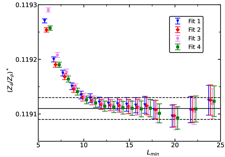
In Fig. 3 we give our results for the fixed point value $(Z_{a}/Z_{p})^{*}$ of the ratio of partition functions using set 1. In comparison with $\omega$, the results for $(Z_{a}/Z_{p})^{*}$ show little dependance on the Ansatz that is used. The final estimate and its error are chosen such that the results of all four fits from $L_{min}=12$ up to $17$ are covered. Fitting set 2, we get consistent results. The final estimates and the errors of the other dimensionless quantities are determined in a similar way. We get

$$(Z_{a}/Z_{p})^{*} = 0.11911(2)\;,$$ (22)

$$(\xi_{2nd}/L)^{*} = 0.547296(26)\;,$$ (23)

$$U_{4}^{*} = 1.094016(12)\;,$$ (24)

$$U_{6}^{*} = 1.281633(33)\;.$$ (25)

Figure 3: Data set 1, i.e. $\lambda=4$, $12.5$, $18.5$, $20$, and $\infty$ for $N=4$. Numerical estimates of $(Z_{a}/Z_{p})^{*}$ obtained from the fits 1, 2, 3, 4, which are discussed in the text, are plotted versus the minimal linear lattice size $L_{min}$ that is taken into account. The solid line gives our final estimate of $(Z_{a}/Z_{p})^{*}$, while the dashed lines indicate the error. Note that the values on the $x$-axis are slightly shifted to reduce overlap of the symbols.

Finally, in table 1 we summarize the estimates of the critical temperature obtained in these fits. Our result for $\lambda=\infty$ is fully consistent with $\beta_{c}=0.935856(2)$ given in ref. Deng06 .

Table 1: Estimates of the inverse critical temperature $\beta_{c}$ for $N=4$.

$\lambda$	$\beta_{c}$
$2.0$	0.7978640(4)
$4.0$	0.85875410(35)
$12.5$	0.90951811(21)
$18.5$	0.91787555(17)
$20$	0.91919685(15)
$\infty$	0.93585450(25)

V.2 The magnetic susceptibility and the critical exponent $\eta$

The magnetic susceptibility at criticality behaves as

$$\chi=aL^{2-\eta}\;\left(1+cL^{-\omega}+...+dL^{-\omega_{NR}}+...\right)+b\;,$$ (26)

where $b$ is the analytic background. Corrections $\propto L^{-n\omega}$ with $n>1$ and further subleading corrections are not explicitly given. In order to enforce criticality, we take $\chi$ at a fixed value of either $Z_{a}/Z_{p}$ or $\xi_{2nd}/L$. To this end we take the fixed point values given in eqs. (22,23). In the following we denote $\chi$ at a fixed value of $Z_{a}/Z_{p}$ or $\xi_{2nd}/L$ by $\bar{\chi}$. In the case of fixing $\xi_{2nd}/L$, there is, compared with eq. (26), an additional correction with an exponent equal to $2$.

We consider the improved susceptibility

$$\bar{\chi}_{imp}=\bar{U}_{4}^{x}\bar{\chi}\;\;,$$ (27)

where the exponent $x$ is tuned such that the leading correction to scaling is eliminated. In previous work, we determined $x$ in a preliminary analysis, and then performed fits by using Ansätze based on eq. (26) with a fixed value of $x$. Here we perform fits with $x$ as free parameter. In appendix A, we discuss how we deal with the fact that $x$ appears on the left side of the equation.

In a first step we performed joint fits for $\lambda=4.0$, $12.5$, $18.5$, $20$, and $\infty$, of $U_{4}^{x}\chi$ at $\xi_{2nd}/L=0.547296$ or $Z_{a}/Z_{p}=0.11911$ fixed, where $x$ is a free parameter. In the case of $\chi$ at $Z_{a}/Z_{p}=0.11911$ we used the Ansatz

$$\bar{\chi}_{imp}=aL^{2-\eta}(1+cL^{-\omega_{NR}})+b\;,$$ (28)

where $a$ and $b$ are free parameters for each value of $\lambda$ separately, while $c$ is the same for all values of $\lambda$. At $L_{min}=10$ we get $\chi^{2}/$DOF$=1.02$. The value that we obtain for $x$ is stable with increasing $L_{min}$. For example, we get $x=-1.67(3)$, $-1.70(3)$, $-1.71(5)$, $-1.72(6)$, and $-1.71(8)$ for $L_{min}=10$, $12$, $14$, $16$, and $18$, respectively. In the following, constructing $\bar{\chi}$ we use $x=-1.7$.

In the case of $\chi$ at $\xi_{2nd}/L=0.547296$ we used the Ansatz

$$\bar{\chi}_{imp}=aL^{2-\eta}(1+cL^{-2}+dL^{-\omega_{NR}})+b\;,$$ (29)

where $a$ and $b$ are free parameters for each value of $\lambda$ separately, while $c$ and $d$ are the same for all values of $\lambda$. Here we find that $\bar{\chi}$, by chance, is only little affected by leading corrections. We find $x\approx-0.07$.

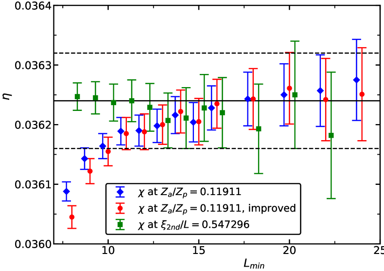
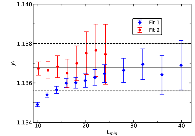
To get the final estimate of $\eta$, we have fitted the data for $\lambda=18.5$ and $20$ jointly. To this end, we use the Ansätze (28,29), but now fixing the value of $x$. In Fig. 4 we give the estimates of $\eta$ as a function of the minimal lattice size $L_{min}$ that is taken into account in the fits. We have fitted $\chi$ at $Z_{a}/Z_{p}=0.11911$ and its improved version by using the Ansatz (28). In both cases, we find $\chi^{2}/$DOF $\approx 1$ and correspondingly an acceptable $p$-value for $L_{min}\geq 10$. Note that here and in the following we consider $0.1\lesssim p\lesssim 0.9$ as acceptable. Instead, $\chi$ at $\xi_{2nd}/L=0.547296$ is fitted by using the Ansatz (29). In the case of $\chi$ at $Z_{a}/Z_{p}=0.11911$, we see that the results differ only by little between the standard and improved version of $\chi$, which is due to the fact that $\lambda=18.5$ and $20$ are close to $\lambda^{*}$. Here we get an acceptable $p$-value for $L_{min}\geq 8$.

Our final estimate

$$\eta=0.03624(8)\;$$ (30)

and the associate error bar are chosen such that the estimates of $\eta$ and their error bars obtained by fitting $\chi$ at $\xi_{2nd}/L=0.547296$ are covered up to $L_{min}=16$. The estimates obtained from $\chi$ at $Z_{a}/Z_{p}=0.11911$ are contained from $L_{min}=11$ up to $22$.

Figure 4: Estimates of $\eta$ from joint fits for $\lambda=18.5$ and $20$ for $N=4$. We give the results of fits for $\chi$ at $Z_{a}/Z_{p}=0.11911$ and its improved version obtained by using the Ansatz (28). Furthermore we give the estimates obtained by fitting $\chi$ at $\xi_{2nd}/L=0.547296$ by using the Ansatz (29). Note that the values on the $x$-axis are slightly shifted to reduce overlap of the symbols. The solid line gives our final estimate and the dashed lines indicate the error.

V.3 The slope of dimensionless quantities and the exponent $\nu$

We have analyzed the slopes of dimensionless quantities at $Z_{a}/Z_{p}=0.11911$ or $\xi_{2nd}/L=0.547296$. We used Ansätze of the type

$$S_{R}=aL^{y_{t}}\;\left(1+\sum_{i}c_{i}L^{-\epsilon_{i}}\right)+bL^{-\omega}\;\;,$$ (31)

where $y_{t}=1/\nu$. The term $bL^{-\omega}$ is due to the fact that the scaling field of the leading correction depends on $\beta$. The derivative of this scaling field with respect to $\beta$ in general does not vanish at $\lambda^{*}$. For a discussion see for example section III of ref. myClock . We ignore leading corrections to scaling that multiply $aL^{y_{t}}$, since we consider good approximations of $\lambda^{*}$ or we consider improved quantities, where leading corrections are suppressed for any $\lambda$.

Here we focus on the slopes of $Z_{a}/Z_{p}$ and $\xi_{2nd}/L$, since their relative statistical error is smaller than that of the Binder cumulants $U_{4}$ and $U_{6}$. Let us first discuss the slope of $Z_{a}/Z_{p}$ at $Z_{a}/Z_{p}=0.11911$. Here we expect only subleading corrections with a correction exponent close to two due to the breaking of the rotational invariance $\propto L^{-\omega_{NR}}$ and the additive term $bL^{-\omega}$. We performed fits by using an Ansatz containing only a correction $\propto L^{-\omega_{NR}}$ and with an Ansatz containing the term $bL^{-\omega}$ in addition. The results obtained for $y_{t}$ by using these two Ansätze, jointly fitting the data for $\lambda=18.5$ and $20$, are plotted in Fig. 5. We get an acceptable $p$-value starting from $L_{min}=11$ for both Ansätze.

Figure 5: Results for the RG-exponent $y_{t}$ of joint fits for $\lambda=18.5$ and $20$ for $N=4$. The slope of $Z_{a}/Z_{p}$ at $Z_{a}/Z_{p}=0.11911$ is fitted by using the Ansatz (31) as discussed in the text. We take either one or two correction terms into account. In the legend, these two choices are referred to by fit 1 or 2. Note that the values on the $x$-axis are slightly shifted to reduce overlap of the symbols. The solid line gives our final estimate and the dashed lines indicate the error.

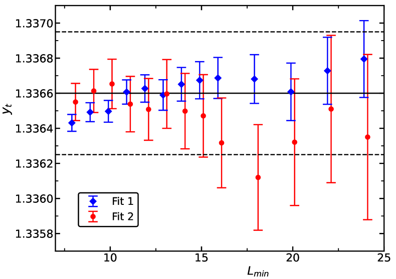
In order to check the effect of leading corrections to scaling on the estimate of $y_{t}$, we perform separate fits for $\lambda=4.0$, $12.5$ and $\infty$. Fitting, taking into account only the correction $\propto L^{-\omega_{NR}}$, for $L_{min}=16$, we get $y_{t}=1.33979(26)$, 1.33680(24), and 1.33574(21) for $\lambda=4.0$, $12.5$ and $\infty$, respectively. We conclude that, given the small amplitude of leading corrections to scaling at $\lambda=18.5$ and $20$, we can neglect the effect of leading corrections to scaling in our final estimate of $y_{t}$, which is based on the data for $\lambda=18.5$ and $20$.

Next we study the slope of $\xi_{2nd}/L$ at $\xi_{2nd}/L=0.547296$. Here we study, also having in mind the analysis of the data for larger values of $N$, similar to the analysis of the magnetic susceptibility, improved versions of the slope. Similar to eq. (27), we multiply by a power of $U_{4}$:

$$\bar{S}_{\xi_{2nd}/L,imp}=\bar{U}_{4}^{x}\bar{S}_{\xi_{2nd}/L}\;.$$ (32)

Furthermore, one might construct an improved slope by combining the slope of $\xi_{2nd}/L$ with that of the Binder cumulant $U_{4}$:

$$\bar{S}_{mix}=\bar{S}_{\xi_{2nd}/L}+x\bar{S}_{U_{4}}\;.$$ (33)

Similar to the analysis of the dimensionless quantities, we performed joint fits for two sets of $\lambda$ values. We consider $\lambda=\infty$, $20$, $18.5$, $12.5$, and $4$. As check, we take a second set, where $\lambda=2$ is added. Also here we used two different types of fits. In the first fit, we used a single correction with $\epsilon_{1}=2$. The additive correction with the exponent $\omega$ is neglected. In the second fit, this correction is present. For both corrections we use eq. (18) as parameterization of the coefficient. Given the present statistical error of the data, we can not resolve a larger number of corrections with $\epsilon\approx 2$.

Analyzing the improved slope (32) we find $x=0.25(15)$ taking into account the two types of fits that we performed. Note that $\chi^{2}/$DOF$=1.20$ is reached for $L_{min}=16$ in the case of fit 1 and $\chi^{2}/$DOF$=1.10$ for $L_{min}=10$ in the case of fit 2. In both cases all values of $\lambda$ are taken into account. The estimates of $y_{t}$ obtained by performing these fits are shown in Fig. 6. We find that the result is fully consistent with that obtained above for $Z_{a}/Z_{p}$.

Figure 6: Results of joint fits for $\lambda=\infty$, $20$, $18.5$, $12.5$, $4$ and $2$ for $N=4$. The improved slope of $\xi_{2nd}/L$ at $\xi_{2nd}/L=0.547296$, eq. (32), is fitted by using the Ansatz (31) as discussed in the text. We take either one or two correction terms into account. In the legend, these two choices are referred to by fit 1 or 2. Note that the values on the $x$-axis are slightly shifted to reduce overlap of the symbols. The solid line and the dashed lines give the result and the error bar obtained above from the slope of $Z_{a}/Z_{p}$.

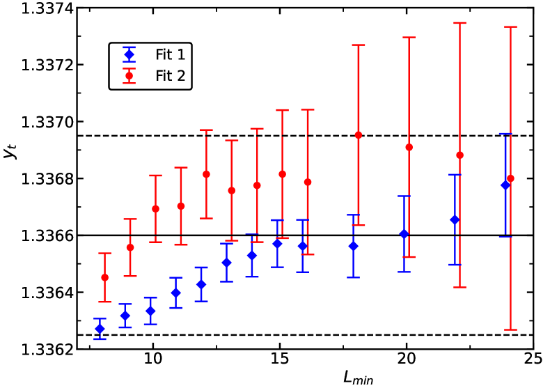
Analyzing the mixed slope (33) we find $x=-0.05(5)$. The results obtained for $y_{t}$ are very similar to those for the improved slope (32).

As our final result we quote the one obtained from the slope of $Z_{a}/Z_{p}$ at $\lambda=18.5$ and $20$

$$y_{t}=1.33660(35)\;,$$ (34)

corresponding to $\nu=0.74817(20)$.

VI The simulations and the analysis of the data for $N=5$

We have simulated at $\lambda=\infty$, $10$, $5$, and $1$. In the case of $\lambda=\infty$ we simulated the lattice sizes $L=8$, $9$, $10$, …, $16$, $18$, $20$, …, $24$, $28$, $32$, …, $40$, $48$, $56$, …, $80$, $100$, and $200$. The number of measurements is decreasing with increasing lattice size $L$. For example, we performed $3.4\times 10^{9}$, $1.2\times 10^{8}$, and $8.5\times 10^{7}$ measurements for $L=10$, $100$, and $200$, respectively. These simulations took about $6.4$ years of CPU time.

For $\lambda=10$ and $5$ we simulated the same set of lattice size as for $\lambda=\infty$ but with a maximal lattice size $L=72$. The number of measurements for each lattice size is a bit smaller than for $\lambda=\infty$. These simulations took about $3.3$ and $2.8$ years of CPU time for $\lambda=10$ and $5$, respectively.

For $\lambda=1$, we simulated the lattice sizes $L=12$, $16$, $20$, …, $48$, $56$, $64$, $72$, and $80$. For example for $L=12$ and $80$, we performed $2.3\times 10^{9}$ and $2.4\times 10^{8}$ measurements, respectively. These simulations took about $6.9$ years of CPU time.

VI.1 The dimensionless quantities

We performed fits by using the same Ansätze as for $N=4$. First we analyzed the data for $\lambda=\infty$, $10$, and $5$ jointly. As check, we have added in a second set of fits the data for $\lambda=1$. In the case of the first set, using the Ansatz (16) with $k_{max}=1$ and the parameterization (17), a reasonable goodness of the fit is reached at $L_{min}=22$ with $\chi^{2}/$DOF$=1.15$ corresponding to $p=0.127$. Using Ansatz (16) with $k_{max}=2$ and the parameterization (18), we get for example $\chi^{2}/$DOF$=1.18$ corresponding to $p=0.039$ for $L_{min}=12$ and $\chi^{2}/$DOF$=0.99$ corresponding to $p=0.515$ for $L_{min}=16$. Adding the data for $\lambda=1$, we get $\chi^{2}/$DOF$=1.07$ corresponding to $p=0.244$ for $L_{min}=18$. Using the Ansatz (16) with $k_{max}=3$ and the parameterization (19), we get $\chi^{2}/$DOF$=1.14$ corresponding to $p=0.080$ for $L_{min}=14$ and $\chi^{2}/$DOF$=1.00$ corresponding to $p=0.470$ for $L_{min}=18$. Below, we refer to these four choices of the data set and the Ansatz as fit $1$, $2$, $3$, and $4$, respectively.

Figure 7: Numerical estimates of the correction exponent $\omega$ for $N=5$ obtained from the fits discussed in the text. Fit 1 and 2 are based on the data for $\lambda=\infty$, $10$ and $5$. In the case of fits 3 and $4$, in addition, $\lambda=1$ is taken into account. In the case of fit 1, we use $k_{max}=1$ and the parameterization (17). In the case of fits 2 and 3 we use $k_{max}=2$ and the parameterization (18), while for fit 4 $k_{max}=3$ and the parameterization (19) is taken. Note that the values on the $x$-axis are slightly shifted to reduce overlap of the symbols. The solid line and the dashed lines give the final result and the error bar.

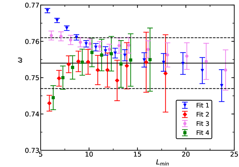
In Fig. 7 we plot the estimates of the correction exponent $\omega$ obtained by fitting as discussed above. As our final result we quote

$$\omega=0.754(7)\;.$$ (35)

This estimate covers fit 1 for $L_{min}=11$ up to $22$, fit 2 for $L_{min}=7$ up to $12$, fit 3 for $L_{min}=9$ up to $22$, fit 4 for $L_{min}=8$ up to $11$ and $13$.

We have determined the fixed point values of the dimensionless quantities in a similar fashion as for $N=4$. We skip a detailed discussion of the analysis. Our results are summarized in table 2.

Next let us discuss the amplitude of leading corrections. For example for fit 4 with $L_{min}=14$, we get $b=-0.00088(21)$, $-0.00870(30)$, $-0.01502(43)$, and $-0.0407(13)$ for $\lambda=\infty$, $10$, $5$ and $1$, respectively. Varying the form the Ansatz (16) we find $b<0$ throughout for $\lambda=\infty$. Assuming that $b$ is a monotonous function of $\lambda$, this implies that for $N=5$ no $\lambda^{*}$ exists. However the amplitude of $b$ at $\lambda=\infty$ is rather small. Therefore in the following analysis of the data, we can regard $\lambda=\infty$ as a reasonable approximation of $\lambda^{*}$.

With increasing $N$ the value of $(Z_{a}/Z_{p})^{*}$ approaches $0$, while $(\xi_{2nd}/L)^{*}$ approaches a finite value. Therefore, going to larger values of $N$, we focus on $\xi_{2nd}/L$ instead of $Z_{a}/Z_{p}$. In particular in the Ansatz (16) we set $a_{\xi_{2nd}/L}=1$ instead of $a_{Z_{a}/Z_{p}}=1$. This way the correction amplitude $b(\lambda)$ for different values of $N$ can be compared more easily. Estimates of $b(\lambda)$, setting $a_{\xi_{2nd}/L}=1$ for $N\geq 5$ are given in table 3.

Our estimates of the inverse critical temperature $\beta_{c}$ are summarized in table 4.

VI.2 The magnetic susceptibility and the exponent $\eta$

First we analyzed the improved magnetic susceptibility, eq. (27), at $\xi_{2nd}/L=0.53691$. Here we used the Ansatz

$$\bar{\chi}_{imp}=aL^{2-\eta}+b\;,$$ (36)

where $a$ and $b$ are free parameters for each value of $\lambda$ and in addition the Ansätze (28,29). We included data for all values of $\lambda$ that we have simulated. In Fig. 8 our results for $\eta$ are plotted versus the minimal lattice size $L_{min}$ that is taken into account. We get acceptable $p$-values starting from $L_{min}=16$, $8$ and $8$ for the Ansätze (36,28,29), respectively. As our final result we take

Figure 8: Estimates of $\eta$ from joint fits for $\lambda=\infty$, $10$, $5$, and $1$ for $N=5$. The data for $\chi_{imp}$ at $\xi_{2nd}/L=0.53691$ are fitted by using the Ansätze (36,28,29). In the legend, these are referred to as fit 1, 2, and 3. Note that the values on the $x$-axis are slightly shifted to reduce overlap of the symbols. The solid line gives our final estimate and the dashed lines indicate the error.

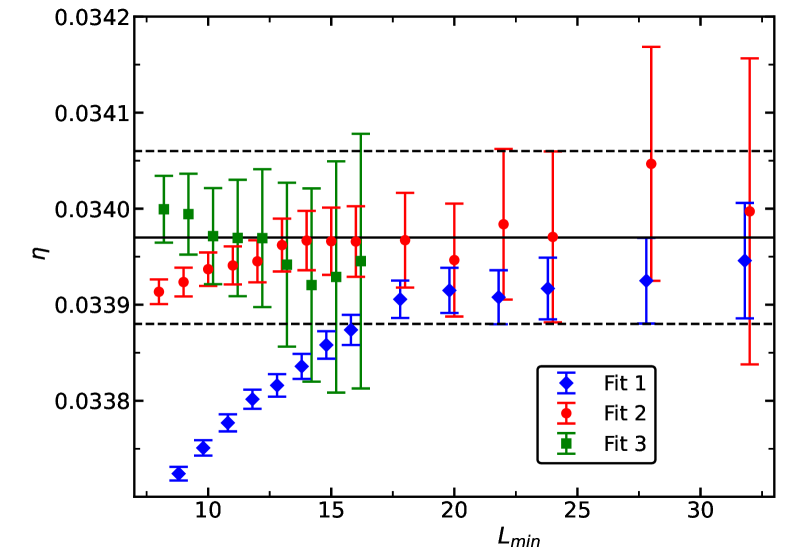
$$\eta=0.03397(9)\;.$$ (37)

Furthermore, we get $x=0.075(25)$. Fixing $Z_{a}/Z_{p}=0.07263$ instead of $\xi_{2nd}/L=0.53691$ we get $\eta=0.03398(11)$ and $x=-2.06(6)$. As a check, we analyzed the data for $\chi$ and $\chi_{imp}$ with $x=0.075$ at $\xi_{2nd}/L=0.53691$ for $\lambda=\infty$ separately. We find that the results for $\eta$ obtained by fitting $\chi$ and $\chi_{imp}$ differ only by a small fraction of the error bar. We find that the results for $\eta$ are fully consistent with eq. (37) that we regard as our final estimate.

VI.3 The slope of dimensionless quantities and the critical exponent $\nu$

First we have analyzed the slope of the ratio of partition functions $Z_{a}/Z_{p}$ at $Z_{a}/Z_{p}=0.07263$. Here we expect subleading corrections proportional to $L^{-\omega_{NR}}$. The corrections due to the additive contribution $bL^{-\omega}$ effectively corresponds to a correction with the exponent $y_{t}+\omega$. Putting in the numerical values $1.282+0.754(7)\approx 2.036$, where we anticipate our estimate of $y_{t}$ given below, we get for $N=5$ a value close to $\omega_{NR}$. Since there is little chance to disentangle these two different corrections in the fit, we use an Ansatz containing a single correction term. The results for the RG-exponent $y_{t}$ obtained from the data for $\lambda=\infty$ are plotted in Fig. 9. Acceptable $p$-values are obtained for $L_{min}\geq 12$. For the Ansatz without any correction, acceptable $p$-values are obtained for $L_{min}\geq 24$. As estimate we take $y_{t}=1.2822(6)$. To get an idea on the effect of the leading correction to scaling, we quote the results obtained for $L_{min}=12$ and the Ansatz containing a correction term proportional to $L^{-\omega_{NR}}$: $y_{t}=1.28224(20)$, $1.28424(27)$, $1.28679(30)$, and $1.29557(24)$ for $\lambda=\infty$, $10$, $5$, and $1$, respectively.

Figure 9: Estimates of $y_{t}$ from fits of the slope of $Z_{a}/Z_{p}$ at $Z_{a}/Z_{p}=0.07263$ for $\lambda=\infty$ and $N=5$ plotted versus the minimal lattice size $L_{min}$ that is taken into account. In the legend, fit 1 refers to an Ansatz without correction term, while fit 2 refers to an Ansatz with a correction proportional to $L^{-\omega_{NR}}$. Note that the values on the $x$-axis are slightly shifted to reduce overlap of the symbols. The solid line gives our preliminary estimate and the dashed lines indicate the error: $y_{t}=1.2822(6)$.

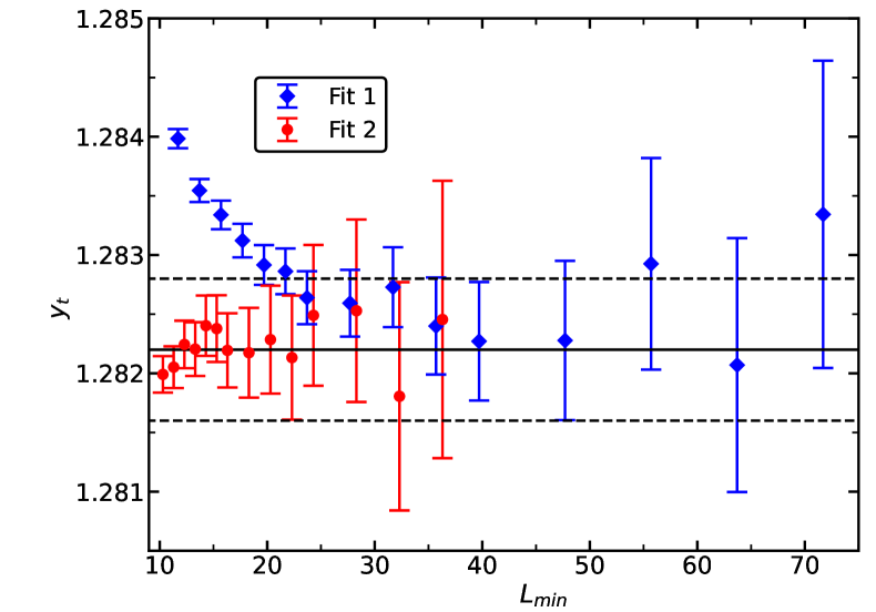
Next we analyze the slope of $\xi_{2nd}/L$ at $\xi_{2nd}/L=0.53691$. Here we expect in addition subleading corrections with the exponents $2-\eta$ and $2$. Since it is virtually impossible to disentangle the subleading corrections here, we performed fits without any corrections and with an Ansatz containing a single correction term proportional to $L^{-2+\eta}$. Our results for $\lambda=\infty$ are given in Fig. 10. Without any correction, we get a acceptable $p$-values for $L_{min}\geq 28$ and including one correction term, we get acceptable $p$-values for $L_{min}\geq 8$.

Figure 10: Estimates of $y_{t}$ from fits of the slope of $\xi_{2nd}/L$ at $\xi_{2nd}/L=0.53691$ for $\lambda=\infty$ and $N=5$ plotted versus the minimal lattice size $L_{min}$ that is taken into account. In the legend, fit 1 refers to an Ansatz without correction term, while fit 2 refers to an Ansatz with a correction proportional to $L^{-2+\eta}$. Note that the values on the $x$-axis are slightly shifted to reduce overlap of the symbols. The solid line gives our preliminary estimate and the dashed lines indicate the error: $y_{t}=1.2818(8)$.

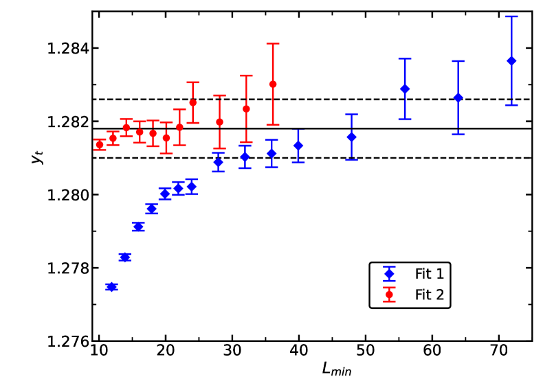
For the fit with a correction term and $L_{min}=16$ we get $y_{t}=1.28171(29)$, $1.28134(33)$, $1.28305(44)$, and $1.28501(35)$ for $\lambda=\infty$, $10$, $5$, and $1$, respectively. We see that the estimate of $y_{t}$ is less effected by leading corrections to scaling than in the case of the slope of $Z_{a}/Z_{p}$ at $Z_{a}/Z_{p}=0.07263$.

As our final estimate we quote

$$y_{t}=1.2818(10)$$ (38)

that covers both preliminary estimates and takes into account that the estimate obtained from the slope of $Z_{a}/Z_{p}$ might be slightly overestimated due to leading corrections to scaling.

As check we analyze the improved slopes, eqs. (32,33), of $\xi_{2nd}/L$ at $\xi_{2nd}/L=0.53691$. First we have analyzed the improved slope, eq. (32). We used an Ansatz without correction term and one with a correction proportional to $L^{-2}$. Note that replacing the correction exponent $2$ by $2-\eta$ or $\omega_{NR}$ changes the estimate of $y_{t}$ only by little. An acceptable goodness of the fits is reach for $L_{min}=28$ and $14$, respectively. The estimates of $y_{t}$ are given in Fig. (11). These estimates are consistent with our final estimate, eq. (38). As estimate of the exponent in eq. (32) we get $x=1.05(20)$.

Figure 11: Estimates of $y_{t}$ from joint fits of the improved slope, eq. (32), of $\xi_{2nd}/L$ at $\xi_{2nd}/L=0.53691$ using the data for $\lambda=\infty$, $10$, $5$, and $1$ for $N=5$. In the legend, fit 1 refers to an Ansatz without correction term, while fit 2 refers to an Ansatz with a correction proportional to $L^{-2}$. Note that the values on the $x$-axis are slightly shifted to reduce overlap of the symbols. The solid line gives our final estimate, eq. (38), and the dashed lines indicate the error.

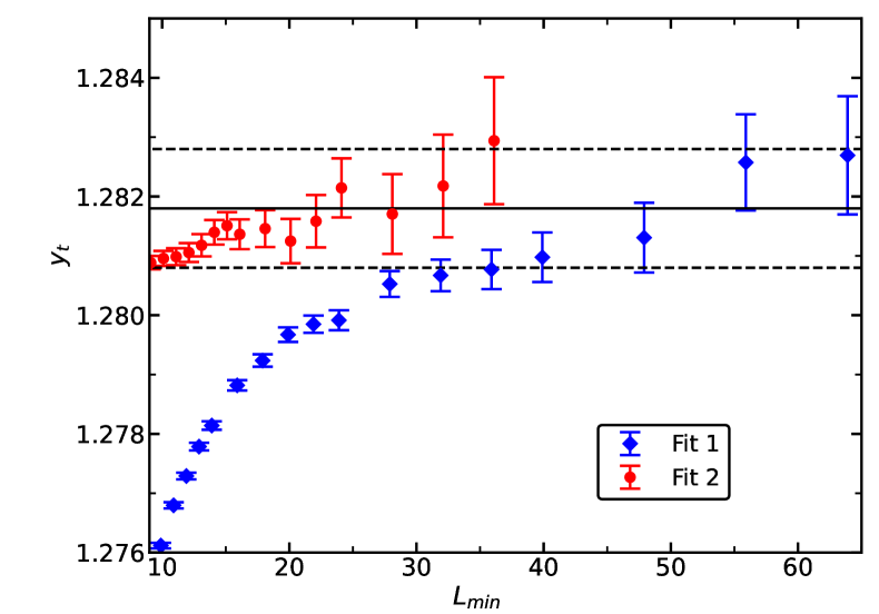
We obtain qualitatively similar result for the other improved quantity, eq. (33).

VII The simulations and the analysis of the data for $N\geq 6$

In addition to $N=4$ and $5$, we have simulated the $\phi^{4}$ model for $N=6$, $8$, $10$, and $12$. In all cases, we simulated at $\lambda=\infty$, $10$, and $5$. For $N=10$, in addition, $\lambda=1$ is considered. The largest lattice size that we simulate for $\lambda=\infty$ is $L=200$, $100$, $100$, and $72$ for $N=6$, $8$, $10$, and $12$, respectively. The statistics for a given lattice size is similar to that of the simulations for $N=4$ and $5$ discussed above. In total we used $20.5$, $13.3$, $24.2$, and $12.9$ years of CPU time for the simulations for $N=6$, $8$, $10$, and $12$, respectively.

VII.1 The dimensionless quantities

For $N\geq 6$, we analyzed dimensionless quantities in a similar way as for $N=4$ and $5$. We fitted our data by using the Ansatz (16). Here we use a parameterization, where $a_{\xi_{2nd/L}}=1$ and $a_{Z_{a}/Z_{p}}$ is a free parameter. Taking into account data for $\lambda=\infty$, $10$ and $5$, we consider either $k_{max}=1$ or $2$ and either the parameterization (17) or (18). In the case of $N=10$, taking into account the data for $\lambda=1$, we also used $k_{max}=3$ and the parameterization (19).

Throughout, the $\chi^{2}/$DOF and the corresponding goodness of the fit as a function of $L_{min}$ behave similar to that discuss for $N=4$ and $5$. Therefore we abstain from a detailed discussion.

Let us first discuss the amplitude of corrections to scaling. In table 3 we give the amplitude $b(\lambda)$ obtained from the fit with $k_{max}=2$ and the parameterization (18) for $L_{min}=12$. Here we abstain from estimating the systematic error of $b(\lambda)$, since we are mainly interested in the qualitative picture. For $N\geq 6$, $b(\infty)>0$, as it is the case of finite $\lambda$. The value of $b(\lambda)$ increases with decreasing $\lambda$. This means that there is no $\lambda^{*}$ and the amplitude of leading corrections to scaling is minimal for $\lambda=\infty$. Furthermore we note that the values of $b(\lambda)$ for a given value of $\lambda$ are similar for $N=8$, $10$, and $12$.

The fixed point values of dimensionless quantities are determined in the same fashion as for $N=4$ and $5$. Our final results are summarized in table 2. We get $\omega=0.758(14)$ and $0.816(16)$ for $N=6$ and $10$, respectively. In the other cases, it is hard to give a reasonable estimate of the error due to a lack of statistics or data for $\lambda=1$. Our results for the inverse critical temperature $\beta_{c}$ are summarized in table 4. To our knowledge, for $\lambda=\infty$, the most accurate results given in the literature for $N=1$, $2$, and $3$ are $\beta_{c}=0.221654628(2)$, ref. Landau18 , $0.45416466(10)$, ref. Xu19 , and $0.693003(2)$, ref. Deng05 , respectively.

Table 2: Estimates of the fixed point values $R^{*}$ of the dimensionless quantities that we have analyzed. For completeness, we have copied the values for $N=4$ from eqs. (22,23,24,25).

$N$	$(Z_{a}/Z_{p})^{*}$	$(\xi_{2nd}/L)^{*}$	$U_{4}^{*}$	$U_{6}^{*}$
4	0.11911(2)	0.547296(26)	1.094016(12)	1.281633(33)
5	0.07263(4)	0.53691(7)	1.069735(25)	1.20860(8)
6	0.04401(4)	0.53038(6)	1.054960(25)	1.16439(8)
8	0.015835(35)	0.5232(1)	1.03825(3)	1.11445(10)
10	0.005610(8)	0.51967(10)	1.02924(2)	1.08753(6)
12	0.00196(1)	0.5178(2)	1.02360(4)	1.07065(10)

Table 3: Estimates of the leading correction amplitude $b(\lambda)$ obtained by fitting with the Ansatz (16), setting $a_{\xi_{2nd}/L}=1$. $k_{max}$ and param. refer to the precise form of the Ansatz. Throughout the minimal linear lattice size that is taken into account is set to $L_{min}=12$. The number in parenthesis gives the statistical error.

$N$	$k_{max}$	param.	$b(\infty)$	$b(10)$	$b(5)$	$b(1)$
5	$2$	eq. (18)	0.00167(34)	0.01844(34)	0.03192(36)
5	$3$	eq. (19)	0.00182(32)	0.0188(4)	0.0325(6)	0.0885(19)
6	$2$	eq. (18)	0.0090(4)	0.0283(6)	0.0426(8)
8	$2$	eq. (18)	0.0180(6)	0.0430(10)	0.0591(14)
10	$2$	eq. (18)	0.0237(8)	0.0557(17)	0.0743(23)
10	$3$	eq. (19)	0.0232(6)	0.0522(12)	0.0687(16)	0.1194(31)
12	$2$	eq. (18)	0.0245(19)	0.0509(47)	0.0641(63)

Table 4: Estimates of the inverse critical temperature $\beta_{c}$ for $N=5$, $6$, $8$, $10$, and $12$ for $\lambda=\infty$, $10$ and $5$. For $N=5$ and $10$, $\lambda=1$ we get $\beta_{c}=0.8044989(5)$ and $1.1665100(13)$, respectively.

$N$\$\lambda$	$\infty$	10	5
5	1.1813639(5)	1.1054374(6)	1.0452357(8)
6	1.4286859(9)	1.2991764(10)	1.2067603(8)
8	1.926761(3)	1.6642478(18)	1.5040374(14)
10	2.427525(4)	2.0039555(35)	1.7744067(20)
12	2.929802(11)	2.322675(5)	2.023970(4)

VII.2 The magnetic susceptibility and the critical exponent $\eta$

Since $(Z_{a}/Z_{p})^{*}$ rapidly decreases with increasing $N$ and its relative error increases with increasing $N$, for $N\geq 6$, we only consider $\chi$ at a fixed value of $\xi_{2nd}/L$. To this end, we take our estimates of $(\xi_{2nd}/L)^{*}$ summarized in table 2.

We perform fits of the improved susceptibility, eq. (27), where the exponent $x$ is a free parameter. We use Ansätze of the form eq. (26). In particular

$$\bar{\chi}_{imp}=a(\lambda)L^{2-\eta}+b(\lambda)\;,$$ (39)

$$\bar{\chi}_{imp}=a(\lambda)L^{2-\eta}(1+cL^{-2})+b(\lambda)\;,$$ (40)

and

$$\bar{\chi}_{imp}=a(\lambda)L^{2-\eta}(1+cL^{-2}+dL^{-\omega_{NR}})+b(\lambda)\;,$$ (41)

where $a(\lambda)$ and $b(\lambda)$ are free parameters for each value of $\lambda$, while $c$ and $d$ are take the same value for all $\lambda$.

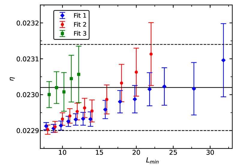
As an example, in Fig. 12, we give estimates of $\eta$ for $N=10$. We get an acceptable $p$-value already for $L_{min}=8$ for all three Ansätze that we consider. The final results for the critical exponent $\eta$ are given in table 5. Results for the exponent in eq. (27) are $x=0.14(4)$, $0.21(6)$, $0.30(5)$, and $0.25(5)$ for $N=6$, $8$, $10$, and $12$, respectively.

Figure 12: Estimates of $\eta$ from joint fits of the improved magnetic susceptibility, eq. (27), at $\xi_{2nd}/L=0.51967$ using the data for $\lambda=\infty$, $10$, and $5$ for $N=10$. In the legend, fits 1, 2, and 3 refer to the Ansätze, eqs. (39,40,41), respectively. Note that the values on the $x$-axis are slightly shifted to reduce overlap of the symbols. The solid line gives our final estimate, and the dashed lines indicate the error.

Table 5: Estimates of $\eta$ and $y_{t}=1/\nu$ for $N=6$, $8$, $10$, and $12$. For a discussion see the text.

$N$	$\eta$	$y_{t}$
6	0.03157(14)	1.2375(9)
8	0.02675(15)	1.1752(10)
10	0.02302(12)	1.1368(12)
12	0.0199(3)	1.1108(17)

VII.3 The slope of dimensionless quantities and the critical exponent $\nu$

We analyzed the improved slope of $\xi_{2nd}/L$, eq. (32), at a fixed value of $\xi_{2nd}/L$. Here we consider the Ansätze

$$\bar{S}_{imp}=a(\lambda)L^{y_{t}}$$ (42)

and

$$\bar{S}_{imp}=a(\lambda)L^{y_{t}}+b(\lambda)L^{-\omega}\;,$$ (43)

where $a(\lambda)$ and $b(\lambda)$ are free parameters for each value of $\lambda$. While $y_{t}$ is a free parameter, we fix $\omega$. To this end, we use the values obtained by the biased Padé approximation discussed below. We checked that varying the value of $\omega$ within plausible errors, the estimates of $y_{t}$ change only by little.

As an example, in Fig. 13 we give estimates of $y_{t}$ for $N=10$. The final results for the RG-exponent $y_{t}$ are given in table 5. Here we get an acceptable $p$-value for $L_{min}\geq 16$ and $8$ for the Ansätze (42,43), respectively. The estimates for the exponent in eq. (32) are $x=1.7(3)$, $3.7(6)$, $5.7(5)$, and $7(1)$ for $N=6$, $8$, $10$, and $12$, respectively.

Figure 13: Estimates of $y_{t}$ from joint fits of the improved slope of $\xi_{2nd}/L$, eq. (32), at $\xi_{2nd}/L=0.51967$ using the data for $\lambda=\infty$, $10$, and $5$ for $N=10$. In the legend, fits 1 and 2 refer to the Ansätze, eqs. (42,43), respectively. Note that the values on the $x$-axis are slightly shifted to reduce overlap of the symbols. The solid line gives our final estimate and the dashed lines indicate the error.

VIII Summary and comparison with other results

We have studied the $O(N)$-symmetric $\phi^{4}$ model on the simple cubic lattice by using Monte Carlo simulations in conjunction with a finite size scaling (FSS) analysis. In the cases $N=1$, $2$, $3$ and $4$ it had been demonstrated before that there is a value $\lambda^{*}$ of the parameter $\lambda$, where leading corrections to scaling vanish. In the large $N$ limit such a $\lambda^{*}$ does not exist CaPe99 . Here we confirm the existence of $\lambda^{*}$ for $N=4$ and provide a more accurate numerical estimate. In contrast, for $N=5$ it is quite clear from the data that no $\lambda^{*}$ exists. In the limiting case $\lambda=\infty$, the amplitude of the corrections is relatively small. Going to larger values of $N$, there is no doubt that there is no $\lambda^{*}$. The minimal amplitude of corrections to scaling is found for the limiting case $\lambda=\infty$. However these corrections can not be ignored in the analysis of the data.

Estimating critical exponents, we focus on $\lambda^{*}$ and $\lambda=\infty$ for $N=4$ and $5$, respectively. For larger values of $N$ we have to deal with leading corrections in a different way. Instead of putting them explicitly into the Ansätze, we use improved observables. The advantage of this approach is that the exponent of the leading correction is not needed.

The $O(N)$-symmetric $\phi^{4}$ theory has been studied by a variety of methods. Lattice models have been studied by using high-temperature (HT) expansions and Monte Carlo (MC) simulations. Field theoretic approaches are the $\epsilon$-expansion and the perturbative expansion in $D=3$ fixed. Accurate results were recently reported by using the functional renormalization group (FRG) method. Recently, accurate estimates of critical exponents were obtained by using the conformal bootstrap method. We have summarized numerical results for the critical exponents $\nu$ and $\eta$ and the correction exponent $\omega$ for $N=4$, $5$ and $10$ in table 6. In particular in the case of field theoretic methods we are not able to cover the large number of works presented in the literature. We focus on recent results. For more extended surveys we refer the reader for example to refs. Kleinert ; PeVi02 .

The authors of ref. Butera computed the HT expansion coefficients of the magnetic susceptibility and the second moment correlation length as rational functions of $N$ for the $O(N)$ invariant model $\phi^{4}$ model in the limit $\lambda=\infty$ on the simple cubic and the body centered cubic (bcc) lattice up to the order $\beta^{21}$. They have analyzed the series by using inhomogeneous differential approximants (DA). In ref. Butera they give numerical estimates for the inverse critical temperature $\beta_{c}$ and the critical exponents $\nu$ and $\gamma=\nu(2-\eta)$ for $N=0$, $1$, $2$, $3$, $4$, $6$, $8$, $10$, and $12$. They give estimates based on an unbiased analysis and an analysis that takes into account a leading correction with the exponent $\theta=\omega\nu$, where the values of $\theta$ are taken from field theory. In table 6 we report only results obtained for the simple cubic lattice. Those obtained for the bcc lattice are similar. Note however that the results of the unbiased and the biased analysis differ by more than the error bars that are quoted. The estimates for the critical exponents essentially agree with ours. However the error is clearly larger than ours. The same observation holds for the estimates of $\beta_{c}$. It would be an interesting exercise to perform a biased analysis of the series by using our values of $\beta_{c}$.

Let us turn to Monte Carlo simulations of lattice models. In ref. Liu12 an $O(N)$-symmetric loop model has been simulated for $N=0$, $0.5$, $1$, $1.5$, $2$, $3$, $4$, $5$ and $10$. The estimates for the critical exponents $\nu$ and $\eta$ are consistent with but less precise than ours. In refs. Deng06 ; ourO5 the $\lambda=\infty$ limit of the model studied here has been simulated for $N=4$ and $5$, respectively. The estimates for the critical exponents $\nu$ and $\eta$ are consistent with but less precise than ours. In refs. O34 ; O234 , similar to the present work, the $\phi^{4}$ model for $N=4$ is studied for various values of $\lambda$. Also here we find that the estimates for the critical exponents are consistent with but less precise than ours.

The authors of ref. Kos15 give rigorous error bars. Indeed our estimates of $\nu$ and $\eta$ for $N=4$ are within the range allowed by the result of ref. Kos15 . The numbers taken from table 2 of ref. CaHaSe16 have a plausible but not rigorous error bar. In the case of the exponent $\nu$ the estimate agrees with ours within the quoted error. In contrast, the estimate of $\omega$ is by roughly twice the error bar larger than ours. Note that similar observations hold when comparing the results of CaHaSe16 for $N=2$ and $3$ with refs. myClock ; myIco .

The $\epsilon$-expansion has been extended recently to 6-loop KoPa17 and to 7-loop Sch18 . In order to get a numerical result for $4-\epsilon=d=3$ a resummation of the series is needed. In the literature one can find a number of different estimates based on the 5-loop series. In particular the estimates of the errors strongly vary. It is beyond our expertise to discuss the different approaches and their respective merits. Here we just like to remark that the estimate of $\nu$ for $N=4$ given in ref. Sha21 clearly differs from our estimate. The same holds for the estimate of $\omega$ for $N=4$ given in ref. KoPa17 .

Throughout we see a good agreement with the results of ref. DePo20 . In the case of $\eta$ our results are considerably more accurate than those of ref. DePo20 .

Table 6: We summarize results for the critical exponents $\nu$ and $\eta$ and the exponent $\omega$ of the leading correction given in the literature. These results were obtained from high-temperature (HT) expansions and Monte Carlo (MC) simulations of lattice models, the conformal bootstrap (CB) method, the $\epsilon$-expansion, the perturbative expansion in $d=3$ and the functional renormalization group. In the case of ref. Butera the authors give estimates of the exponents $\nu$ and $\gamma$. Here we have computed $\eta=2-\gamma/\nu$. Since it is unclear how the error propagates, we abstain from quoting one. For a discussion see the text.

$N$	method	year	Ref	$\nu$	$\eta$	$\omega$
4	HT	1997	Butera	0.750(3)	0.0347	-
4	HT $\theta$-biased	1997	Butera	0.759(3)	0.0356	-
4	MC	2001	O34	0.749(2)	0.0365(10)	-
4	MC	2006	Deng06	0.7477(8)	0.0360(4)	-
4	MC	2011	O234	0.750(2)	0.0360(3)	-
4	MC	2012	Liu12	0.7508(39)	0.034(4)	-
4	MC	2021	this work	0.74817(20)	0.03624(8)	0.755(5)
4	CB	2015	Kos15	0.7472(87)	0.0378(32)	-
4	CB	2016	CaHaSe16	0.7508(34)	-	0.817(30)
4	$\epsilon$, 5-loop	1998	GuZi	0.737(8)	0.036(4)	0.795(30)
4	$d=3$-exp	1998	GuZi	0.741(6)	0.0350(45)	0.774(20)
4	$\epsilon$, 6-loop	2017	KoPa17	0.7397(35)	0.0366(4)	0.794(9)
4	$\epsilon$, 7-loop	2021	Sch18 ; Sha21	0.74425(32)	0.03670(38)	0.7519(13)
4	FRG	2020	DePo20	0.7478(9)	0.0360(12)	0.761(12)
5	MC	2005	ourO5	0.779(3)	0.034(1)	-
5	MC	2012	Liu12	0.784(7)	0.034(6)	-
5	MC	2021	this work	0.7802(6)	0.03397(9)	0.754(7)
5	FRG	2020	DePo20	0.7797(9)	0.0338(11)	0.760(18)
10	HT	1997	Butera	0.867(4)	0.0254	-
10	HT $\theta$-biased	1997	Butera	0.894(4)	0.0280	-
10	MC	2012	Liu12	0.876(12)	0.028(6)	-
10	MC	2021	this work	0.8797(9)	0.02302(12)	0.816(16)
10	FRG	2020	DePo20	0.8776(10)	0.0231(6)	0.807(7)

In table 6 we have taken $N=4$, $5$ and $10$ as examples. Our results for the critical exponents for $N=6$, $8$, and $12$ can be found in table 5. In the Appendix B we interpolate our results by using Padé approximants of extended large $N$ series.

IX Acknowledgement

This work was supported by the Deutsche Forschungsgemeinschaft (DFG) under the grants HA 3150/5-1 and HA 3150/5-2.

Appendix A Fits with a free parameter on the left hand side of the equation

We study the improved magnetic susceptibility and improved slopes, eqs. (27,32). These can be written as

$$\bar{Y}_{imp}=\bar{U}_{4}^{x}\bar{Y},$$ (44)

where $x$ should be tuned such that leading corrections to scaling are eliminated and $Y$ represents either the magnetic susceptibility or a slope. To this end we intend to perform a fit with $x$ as free parameter.

$$\bar{Y}_{imp}(x,L,\lambda)=A(L,\lambda,\{P\})\;,$$ (45)

where the Ansatz $A(L,\lambda,\{P\})$ is given for example by eqs. (36,28,29) in the case of the magnetic susceptibility and $\{P\}$ is the set of free parameters of the Ansatz. In particular, $A(L,\lambda,\{P\})$ should not contain terms that represent the leading correction to scaling. We intend to perform the fit by using the function optimize.curve_fit() of the optimize package of python. The problem is that the parameter $x$ is on the left side of eq. (45). In order to deal with this problem, we divide eq. (45) by $\bar{Y}_{imp}$ on both sides of the equation. Now we treat $\bar{U}_{4}$ and $\bar{Y}$ along with $L$ as $X$ and the value of $y$ is equal to $1$. As statistical error $\epsilon(y)$ of $y$ we assume $\epsilon(y)=\epsilon(\bar{Y}_{imp})/\bar{Y}_{imp}$. In order to determine the statistical error of $\bar{Y}_{imp}$, we take into account the covariance of $\bar{Y}$ and $\bar{U}_{4}$. It remains the problem that $x$ is not know a priori. Therefore we proceed iteratively. First the error is computed for an initial guess of $x$, then for the first result of the fit. Typically we get a stable result after a few iterations. Computing the statistical error of $\bar{Y}_{imp}$, we have neglected that $x$ has a statistical error. Therefore, in general, we regard the approach as an ad hoc approach. In the analysis of our data for $N=4$ and $5$, we have benchmarked the results for critical exponents obtained by using the procedure discussed here with results obtained from standard fits of data for $\lambda$-values close to $\lambda^{*}$. Therefore we regard the estimates of the error obtained here as reliable.

Appendix B Interpolation with large $N$

The critical exponents $\nu$ and $\eta$ and the correction exponent $\omega$ have been computed by using the large $N$ expansion Vasil ; Kondor ; Abe ; BrGrKr96 . Here we give the series as collected in chapter 20 of the book Kleinert :

$$\eta = \frac{8}{3\pi^{2}}\frac{1}{N}-\frac{8}{3}\left(\frac{8}{3\pi^{2}}\right)^{2}\frac{1}{N^{2}}-\left[\frac{797}{18}-\left(27\log(2)-\frac{61}{4}\right)\zeta(2)+\frac{189}{4}\zeta(3)\right]\left(\frac{8}{3\pi^{2}}\right)^{3}\frac{1}{N^{3}}+O(N^{-4})$$ (46)

$$= 0.27018982305\frac{1}{N}-0.1946734413\frac{1}{N^{2}}-1.8812345072\frac{1}{N^{3}}+O(N^{-4})\;,$$

where we have evaluated the coefficients to get a better idea of their magnitude. The exponent of the correlation length

$$\nu = 1-4\frac{8}{3\pi^{2}}\frac{1}{N}-\left[\frac{9}{2}\pi^{2}-\frac{56}{3}\right]\left(\frac{8}{3\pi^{2}}\right)^{2}\frac{1}{N^{2}}+O(N^{-3})$$ (47)

$$= 1-1.0807592922\frac{1}{N}-1.8795637876\frac{1}{N^{2}}+O(N^{-3})$$

and correction exponent

$$\omega = 1-8\frac{8}{3\pi^{2}}\frac{1}{N}-2\left[\frac{9}{2}\pi^{2}-\frac{104}{3}\right]\left(\frac{8}{3\pi^{2}}\right)^{2}\frac{1}{N^{2}}+O(N^{-3})$$ (48)

$$= 1-2.1615185844\frac{1}{N}-1.4230462800\frac{1}{N^{2}}+O(N^{-3})\;.$$

As stated in the literature, evaluating the series naively or by using Padé approximants, numerically useful results can be expected at best for $N\gtrapprox 10$.

Here we like to extend the series by one or two orders, where the additional coefficients are determined by fitting the numerical results for $N=4$, $5$, $6$, $8$, $10$, and $12$ obtained here with Padé approximants of the extended series. We are aiming at a reasonable interpolation for $N=7$, $9$, $11$, and for $N$ somewhat larger than $12$. We used a standard $\chi^{2}$ minimization. Interpreting the result, one has to keep in mind that the error that we quote for the exponents is partially of systematic nature.

In the case of $\eta$ we get an acceptable fit down to $N=8$ for adding a $c_{4}N^{-4}$ term and a $[1,3]$ Padé approximant. As result for the coefficient we get $c_{4}=-4.78(84)$. Adding a $c_{4}N^{-4}$ and a $c_{5}N^{-5}$ term, we get acceptable fits down to $N=5$ by using $[0,5]$ or $[3,2]$ approximants. For the $[1,4]$ Padé approximant we get an acceptable fit even down to $N=4$. The estimates of $c_{4}$ and in particular of $c_{5}$ differ considerably between the different Padé approximants that we used. The estimates of $c_{4}$ and $c_{5}$ and the associated covariance matrices are contained in a Python3 script that we provide as supplemental material. This Python script computes $\eta$ for $N\geq 5$ based on the Padé approximants discussed here.

In the case of $\nu$ and $\omega$ we performed similar fits. Also here, the results are given in Python3 scripts that produce estimates of $\nu$ and $\omega$ for $N\geq 5$.

References

- (1) M. N. Barber, Finite-size Scaling in Phase Transitions and Critical Phenomena, Vol. 8, eds. C. Domb and J. L. Lebowitz, (Academic Press, 1983).
- (2) K. G. Wilson and J. Kogut, The renormalization group and the -expansion, Phys. Rep. C 12, 75 (1974).
- (3) M. E. Fisher, The renormalization group in the theory of critical behavior, Rev. Mod. Phys. 46, 597 (1974).
- (4) M. E. Fisher, Renormalization group theory: Its basis and formulation in statistical physics, Rev. Mod. Phys. 70, 653 (1998).
- (5) H. Kleinert and V. Schulte-Frohlinde, Critical Properties of -Theories, (World Scientific, Singapore 2001).
- (6) A. Pelissetto and E. Vicari, Critical Phenomena and Renormalization-Group Theory, [arXiv:cond-mat/0012164], Phys. Rept. 368, 549 (2002).
- (7) F. Kos, D. Poland, D. Simmons-Duffin, and A. Vichi, Precision Islands in the Ising and Models, [arXiv:1603.04436], JHEP 08 (2016) 036.
- (8) D. Simmons-Duffin, The Lightcone Bootstrap and the Spectrum of the 3d Ising CFT, [arXiv:1612.08471], JHEP 03 (2017) 086.
- (9) S. M. Chester, W. Landry, J. Liu, D. Poland, D. Simmons-Duffin, N. Su, and A. Vichi, Carving out OPE space and precise model critical exponents, [arXiv:1912.03324], JHEP 06 (2020) 142.
- (10) Sh. M. Chester, W. Landry, J. Liu, D. Poland, D. Simmons-Duffin, N. Su, and A. Vichi, Bootstrapping Heisenberg Magnets and their Cubic Instability, [arXiv:2011.14647], Phys. Rev. D 104, 105013 (2021).
- (11) F. Kos, D. Poland, D. Simmons-Duffin, and A. Vichi, Bootstrapping the archipelago, [arXiv:1504.07997], JHEP 11 (2015) 106.
- (12) A. C. Echeverri, B. von Harling, and M. Serone, The effective bootstrap, [arXiv:1606.02771], J. High Energ. Phys. 2016, 97 (2016).
- (13) D. Poland, S. Rychkov, and A. Vichi, The Conformal Bootstrap: Theory, Numerical Techniques, and Applications [arXiv:1805.04405], Rev. Mod. Phys. 91, 15002 (2019).
- (14) M. V. Kompaniets and E. Panzer, Minimally subtracted six-loop renormalization of -symmetric theory and critical exponents, [arXiv:1705.06483], Phys. Rev. D 96, 036016 (2017).
- (15) O. Schnetz, Numbers and functions in quantum field theory, [arXiv:1606.08598], Phys. Rev. D 97, 085018 (2018).
- (16) A. M. Shalaby, Critical exponents of the -symmetric model from the hypergeometric-Meijer resummation, [arXiv:2005.12714], Eur. Phys. J. C 81, 87 (2021).
- (17) V. Abhignan and R. Sankaranarayanan, Continued functions and perturbation series: Simple tools for convergence of diverging series in -symmetric field theory at weak coupling limit, [arXiv:2006.12064], Journal of Statistical Physics 183, 4 (2021).
- (18) G. De Polsi, I. Balog, M. Tissier, and N. Wschebor, Precision calculation of critical exponents in the universality classes with the nonperturbative renormalization group, [arXiv:2001.07525], Phys. Rev. E 101, 042113 (2020).
- (19) N. Dupuis, L. Canet, A. Eichhorn, W. Metzner, J.M. Pawlowski, M. Tissier, and N. Wschebor, The nonperturbative functional renormalization group and its applications, [arXiv:2006.04853], Physics Reports 910, 1 (2021).
- (20) A. M. Ferrenberg, J. Xu, D. P. Landau, Pushing the limits of Monte Carlo simulations for the three-dimensional Ising model, [arXiv:1806.03558], Phys. Rev. E 97, 043301 (2018).
- (21) M. Hasenbusch, Restoring isotropy in a three-dimensional lattice model: The Ising universality class, [arXiv:2105.09781], Phys. Rev. B 104, 014426 (2021).
- (22) W. Xu, Y. Sun, J.-P. Lv, and Y. Deng, High-precision Monte Carlo study of several models in the three-dimensional U(1) universality class, [arXiv:1908.10990], Phys. Rev. B 100, 064525 (2019).
- (23) M. Hasenbusch, Monte Carlo study of an improved clock model in three dimensions, [arXiv:1910.05916], Phys. Rev. B 100, 224517 (2019).
- (24) M. Hasenbusch, Monte Carlo study of a generalized icosahedral model on the simple cubic lattice, [arXiv:2005.04448], Phys. Rev. B 102, 024406 (2020).
- (25) M. Moshe and J. Zinn-Justin, Quantum Field Theory in the Large N Limit: a review, [arXiv:hep-th/0306133], Phys. Rept. 385, 69 (2003).
- (26) M. Campostrini, M. Hasenbusch, A. Pelissetto, P. Rossi, and E. Vicari, Critical behavior of the three-dimensional XY universality class, [arXiv:cond-mat/0010360], Phys. Rev. B 63, 214503 (2001).
- (27) J. H. Chen, M. E. Fisher and B. G. Nickel, Unbiased Estimation of Corrections to Scaling by Partial Differential Approximants, Phys. Rev. Lett. 48, 630 (1982).
- (28) M. E. Fisher and J. H. Chen, The validity of hyperscaling in three dimensions for scalar spin systems, J. Physique (Paris) 46, 1645 (1985).
- (29) H. W. J. Blöte, E. Luijten and J. R. Heringa, Ising universality in three dimensions: a Monte Carlo study, [arXiv:cond-mat/9509016], J. Phys. A: Math. Gen. 28, 6289 (1995).
- (30) H. G. Ballesteros, L. A. Fernández, V. Martín-Mayor, and A. Muñoz Sudupe, Finite Size Scaling and “perfect” actions: the three dimensional Ising model, [arXiv:hep-lat/9805022], Phys. Lett. B 441, 330 (1998).
- (31) M. Hasenbusch, K. Pinn, and S. Vinti, Critical Exponents of the 3D Ising Universality Class From Finite Size Scaling With Standard and Improved Actions, [arXiv:hep-lat/9806012], Phys. Rev. B 59, 11471 (1999).
- (32) M. Campostrini, A. Pelissetto, P. Rossi and E. Vicari, Improved high-temperature expansion and critical equation of state of three-dimensional Ising-like systems, [arXiv:cond-mat/9905078], Phys. Rev. E 60, 3526 (1999).
- (33) M. Hasenbusch, A Monte Carlo study of leading order scaling corrections of theory on a three dimensional lattice, [arXiv:hep-lat/9902026], J. Phys. A 32, 4851 (1999).
- (34) M. Campostrini, M. Hasenbusch, A. Pelissetto, and E. Vicari, The critical exponents of the superfluid transition in He4, [arXiv:cond-mat/0605083], published as Theoretical estimates of the critical exponents of the superfluid transition in He4 by lattice methods, Phys. Rev. B 74 (2006) 144506.
-
(35)
M. Hasenbusch and E. Vicari,
Anisotropic perturbations in three-dimensional O(N)-symmetric vector
models,
[arXiv:1108.0491], Phys. Rev. B 84, 125136 (2011).
- (36) M. Hasenbusch, A. Pelissetto and E. Vicari, Instability of the multicritical behavior in the theory of high-Tc superconductors, [arXiv:cond-mat/0502327], Phys. Rev. B 72, 014532 (2005).
- (37) M. Campostrini, A. Pelissetto, P. Rossi, and E. Vicari, Two-point correlation function of three-dimensional O(N) models: The critical limit and anisotropy, [arXiv:cond-mat/9705086], Phys. Rev. E 57, 184 (1998).
- (38) R.H. Swendsen and J.-S. Wang, Nonuniversal critical dynamics in Monte Carlo simulations, Phys. Rev. Lett. 58, 86 (1987).
- (39) U. Wolff, Collective Monte Carlo Updating for Spin Systems, Phys. Rev. Lett. 62, 361 (1989).
(40)
M. Saito and M. Matsumoto,
“SIMD-oriented Fast Mersenne Twister:
a 128-bit Pseudorandom Number Generator”,
in
Monte Carlo and Quasi-Monte Carlo Methods 2006,
edited by A. Keller, S. Heinrich, H. Niederreiter, (Springer, 2008);
M. Saito, Masters thesis, Math. Dept., Graduate School of science,
Hiroshima University, 2007.
The source code of the program is provided at
http://www.math.sci.hiroshima-u.ac.jp/~m-mat/MT/SFMT/index.html -
(41)
https://prng.di.unimi.it/ - (42) D. Blackman and S. Vigna, Scrambled Linear Pseudorandom Number Generators, [arXiv:1805.01407], ACM Trans. Math. Softw. 47, 36 (2021).
(43)
https://www.pcg-random.org/posts/does-it-beat-the-minimal-standard.html -
(44)
https://de.wikipedia.org/wiki/KISS_(Zufallszahlengenerator) - (45) P. Virtanen, R. Gommers, T. E. Oliphant et al., SciPy 1.0–Fundamental Algorithms for Scientific Computing in Python, [arXiv:1907.10121], Nature Methods 17, 261 (2020).
- (46) J. D. Hunter, ”Matplotlib: A 2D Graphics Environment, Computing in Science & Engineering 9, 90 (2007).
- (47) Y. Deng, Bulk and surface phase transitions in the three-dimensional spin model, Phys. Rev. E 73, 056116 (2006).
- (48) Y. Deng, H. W. J. Blöte, and M. P. Nightingale, Surface and bulk transitions in three-dimensional models, [arXiv:cond-mat/0504173], Phys. Rev. E 72, 016128 (2005).
- (49) P. Butera and M. Comi, -vector spin models on the sc and the bcc lattices: a study of the critical behavior of the susceptibility and of the correlation length by high temperature series extended to order , [arXiv:hep-lat/9703018], Phys. Rev. B 56, 8212 (1997).
- (50) Q. Liu, Y. Deng, T. M. Garoni, and H. W. J. Blöte, The loop model on a three-dimensional lattice, [arXiv:1112.5647], Nucl. Phys. B, 859, 107 (2012).
- (51) M. Hasenbusch, Eliminating leading corrections to scaling in the 3-dimensional O(N)-symmetric model: and , [cond-mat/0010463], J. Phys. A 34, 8221 (2001).
- (52) R. Guida and J. Zinn-Justin, Critical exponents of the N vector model, [arXiv:cond-mat/9803240], J. Phys. A 31, 8103 (1998).
- (53) R. Abe, Critical exponent up to for the three-dimensional system with short-range interaction, Prog. Theor. Phys. 49, 1877 (1973); Y. Okabe, M. Oku and R. Abe, expansion up to order . I: Equation of state and correlation function, Prog. Theor. Phys. 59, 1825 (1978); Y. Okabe and M. Oku, expansion up to order . II: Critical exponent for , Prog. Theor. Phys. 60, 1277 (1978); Expansion Up to Order . IV: Critical Amplitude Ratio , 61, 443 (1979).
- (54) I. Kondor and T. Temesvári, Critical indices to for a three dimensional system with short range forces, J. Phys. Lett. (Paris) 39, L-99; L-415 (1978); Calculation of critical exponents to Phys. Rev. B 21, 260 (1980).
- (55) A. N. Vasil’ev, Yu. M. Pis’mak and J.R. Honkonen, Simple method of calculating the critical indices in the expansion, Theor. Math. Phys. 46, 157 (1981); Expansion: Calculation of the exponents and in the order for arbitrary number of dimensions, Theor. Math. Phys. 47, 465 (1981); Expansion: Calculation of the exponent in the order by the Conformal Bootstrap Method, Theor. Math. Phys. 50, 127 (1982).
- (56) D. J. Broadhurst, J. A. Gracey, and D. Kreimer, Beyond the triangle and uniqueness relations: non-zeta counterterms at large from positive knots, [arXiv:hep-th/9607174], Z. Phys. C 75, 559 (1997).