Identification of Subgroups With Similar Benefits in Off-Policy Policy Evaluation

Abstract

Off-policy policy evaluation methods for sequential decision making can be used to help identify if a proposed decision policy is better than a current baseline policy. However, a new decision policy may be better than a baseline policy for some individuals but not others. This has motivated a push towards personalization and accurate per-state estimates of heterogeneous treatment effects (HTEs). Given the limited data present in many important applications, individual predictions can come at a cost to accuracy and confidence in such predictions. We develop a method to balance the need for personalization with confident predictions by identifying subgroups where it is possible to confidently estimate the expected difference in a new decision policy relative to a baseline. We propose a novel loss function that accounts for uncertainty during the subgroup partitioning phase. In experiments, we show that our method can be used to form accurate predictions of HTEs where other methods struggle.

1 Introduction

Recent advances in technology and regulations around them have enabled the collection of an unprecedented amount of data of past decisions and outcomes in different domains such as health care, recommendation systems, and education. This offers a unique opportunity to learn better decision-making policies using the observational data. Off-policy policy evaluation (OPE) is concerned with estimating the value of a proposed policy (evaluation policy) using the data collected under a different policy (behaviour policy). Estimating the value of an evaluation policy before deployment is essential, especially when interacting with the environment is expensive, risky, or unethical, such as in health care  (Gottesman et al., 2019). Fortunately, the reinforcement learning (RL) community has developed different methods and theories focused on OPE, e.g. Jiang and Li (2016); Thomas and Brunskill (2016); Kallus and Uehara (2020).

OPE has been used extensively in the literature to demonstrate the superiority of a proposed evaluation policy relative to the baseline (behaviour) policy e.g. Komorowski et al. (2018); however, the evaluation policy may be better than the behaviour policy for some individuals but not others. Hence, only looking at the estimated value of the evaluation policy before deployment, may be misleading. In the non-sequential setting, a growing literature has focused on personalization and estimation of heterogeneous treatment effect (HTE), the individual-level differences in potential outcomes under the proposed evaluation policy versus the behaviour policy (Athey et al., 2019; Nie and Wager, 2017).

However, due to the limited availability of data and a long horizon, the goal of personalization for each individual can be unrealistic, especially in sequential settings. In practice, individual predictions of treatment effects in these settings can be inaccurate and highly uncertain, providing no actionable information.

In this paper, we aim to provide actionable information to domain experts. Specifically, we ask "What subgroups of individuals can we confidently predict that will be significantly benefited or harmed by adopting the evaluation policy?". Asking this question instead of "What is the treatment effect for each individual?" allows us to group individuals that have similar treatment effects together, pool the data, and make predictions that are both more accurate and confident. This information can be used by a domain expert (human-in-the-loop) to make informed decisions before deploying the RL system, or be used for the interpretability of the OPE. For example, a clinician can take a look at the groups and decide if the predicted benefit or harm is in accordance with their clinical intuition.

We propose using a loss function similar to non-sequential setting (Athey and Imbens, 2016) and greedily minimize it with recursive partitioning, similar to the classification and regression trees (CART). Estimation of the naive loss function can be too noisy and often results in over-splitting, yielding too many subgroups and inaccurate or uncertain prediction. We make two main changes to the naive loss function. First we mitigate the issue of noisy estimation by proposing a novel upper bound to the loss function that is stable and can be efficiently calculated.

Additionally, by taking into account what clinicians believe is relevant for decision making, we incorporate a regularization term that incentivizes recursive partitioning to find subgroups with relevant treatment effects. This term can be directly specified by a clinician, and allows for better incorporation of medical experts into the evaluation process. For example, a clinician may consider an increase of 10% in survival rate relevant, so only subgroups with a confident prediction of 10% decrease or increases in survival rate will provide actionable information. Combining these two additions, we propose a new loss function that can be efficiently computed.

On a simulated example of sepsis management (Oberst and Sontag, 2019) we show how our proposed method can be used to find subgroups with significant treatment effect, providing more accurate and confident predictions. Additionally, we apply our method to the sepsis cohort of the MIMIC III ICU dataset (Johnson et al., 2016), and illustrate how it can be used to identify subgroups in which a new decision policy may be beneficial or harmful relative to the standard approach. We also investigate the interpretability of our findings through a discussion with an ICU intensivist.

2 Related Work

Estimating the value of a new decision policy arise in many different applications, such as personalized medicine (Obermeyer and Emanuel, 2016), bandits (Dudík et al., 2011) and sequential decision makings (Thomas and Brunskill, 2016). The RL community has developed different methods and theories for off-policy policy evaluation (OPE) in sequential setting. These methods mostly fall into different categories: importance sampling (Precup, 2000), model based and doubly robust methods (Dudík et al., 2011; Thomas and Brunskill, 2016; Jiang and Li, 2016). These methods can be used along with our algorithm to estimate group treatment effect for a particular group; however, these methods do not offer a way to perform partitioning.

In non-sequential settings, a growing number of literature seek to estimate heterogeneous treatment effect (HTE) using different approaches. Imai and Ratkovic (2014) uses the LASSO to estimates the effect of treatments, Shalit et al. (2017) uses neural networks and offers generalization bound for individual treatment effect (ITE). Nie and Wager (2017) proposed two step estimation procedure using double machine learning and orthogonal moments (Chernozhukov et al., 2018) that can be applied on observational data to infer HTEs, and recently, Lee et al. (2020) suggests a robust partitioning algorithm by inducing homogeneity in groups. However, these methods were developed for non-sequential settings and naïvely applying them to sequential setting will result in predictions with low accuracy and high uncertainty. Our work draws close parallel to methods using recursive partitioning to estimate HTEs (Athey and Imbens, 2016; Athey et al., 2019), but those works suffer from over-splitting the feature space in sequential setting due to noisy estimation of the loss function. We propose a different loss function that can be better estimated given the lack of data and incorporate domain expert knowledge.

3 Setting and Background

We consider an episodic stochastic decision processes with a finite action space $\mathcal{A}$, continuous state space $\mathcal{X}\in\mathbb{R}^{M}$, reward function $R:\mathcal{X}\times\mathcal{A}\rightarrow[0,R_{max}]$ and discount factor $\gamma\in[0,1]$. A policy $\pi$ maps the state space to a probability distribution over the action space, and we assume each episode lasts at most $H$ steps. A set of trajectories $\mathcal{T}=\{\tau_{1},\dots,\tau_{N}\}$ is provided. Each trajectory $\tau_{i}$ consists of a state $x_{t}$, action $a_{t}$ and observed reward $r_{t}$ at step $t$, $\tau_{i}=\{x^{i}_{0},a^{i}_{0},r^{i}_{0},\dots,x^{i}_{H}\}$. Actions are generated by following a known behaviour policy $\pi_{b}$, $a_{t}\sim\pi_{b}(s_{t})$. We denote the evaluation policy by $\pi_{e}$.

4 Framework for Subgroup Identification

Our focus is to robustly quantify the expected benefit or cost of switching from a behavior policy to a proposed evaluation policy on subsets of the population. To do so it is helpful to extend the standard notion of the treatment effect to the (sequential decision) policy treatment effect. We define the individual treatment effect $t(x;\pi_{e},\pi_{b})$ for a possible initial state $x$ as

$$t(x;\pi_{e},\pi_{b})=\mathbb{E}_{\pi_{e}}\left[\sum_{t=0}^{H}\gamma^{t}r_{t}|x_{0}=x\right]-\mathbb{E}_{\pi_{b}}\left[\sum_{t=0}^{H}\gamma^{t}r_{t}|x_{0}=x\right].$$ (1)

Before we introduce our definition of group treatment effects, we first define a partitioning over the state space by $L=\{l_{1},\dots,l_{M}\}\in\Pi$, such that $\bigcup\limits_{i=1}^{M}l_{i}=\mathcal{X}$ and $\forall i,j:\quad l_{i}\bigcap l_{j}=\emptyset$. Define the partition function $l(x;L)=l_{i}$ such that $x\in l_{i}$. Given a partitioning $L$, partition-value function for a policy $\pi$ can be defined as:

$$v(x;L,\pi)=\underset{{\begin{subarray}{c}x^{\prime}\sim\mathcal{X}\\ a\sim\pi(.|x^{\prime})\end{subarray}}}{\mathbb{E}}\left[\sum_{t=0}^{H}\gamma^{t}r_{t}|x_{0}=x^{\prime},x^{\prime}\in l(x;L)\right]$$

Using this function we can define group treatment effect, similar to the individual treatment effect as,

$$T(x;L,\pi_{b},\pi_{e})=v(x;L,\pi_{e})-v(x;L,\pi_{b})$$ (2)

note that group treatment effect is constant within every $l_{i}$, and we refer to each $l_{i}$ as a group. With little abuse of notation we denote the individual treatment effect by $t(x)$ and group treatment effect by $T(x;L)$ and may interchangeably use group and subgroup.

4.1 Group treatment effect estimator

Given a partition $L$, a set of trajectories $\mathcal{T}$, the behaviour policy $\pi_{b}$ and an evaluation policy $\pi_{e}$ the following estimator defines the group treatment effect estimator for an initial state $x$ over a dataset $\mathcal{D}=\{(x_{0},\rho_{0},g_{0}),\dots,(x_{N},\rho_{N},g_{N})\}$,

$$\hat{T}(x;L)=\frac{1}{\left|\{x_{i}|x_{i}\in l(x;L)\}\right|}\sum_{i|x_{i}\in l(x;L)}(\rho_{i}g_{i}-g_{i})$$ (3)

Where, $x_{i}=x_{0}^{i}$ is the initial state of a trajectory $\tau_{i}$, $g_{i}$ is the discounted return $g_{i}=\sum_{t=0}^{H}\gamma^{t}r^{i}_{t}$ and $\rho_{i}$ is the importance sampling ratio $\rho_{i}=\prod_{t=0}^{H}\frac{\pi_{e}(a^{i}_{t}|x^{i}_{t})}{\pi_{b}(a^{i}_{t}|x^{i}_{t})}$. It is straightforward to show that $\hat{T}(x;L)$ is an unbiased estimator of $T(x;L)$ in every group.

Following much of the literature (Athey and Imbens, 2016; Thomas and Brunskill, 2016) we focus on the MSE criteria to rank different estimators defined by different partitioning; however, as explained later, we modify this loss in multiple ways to account for our goal.

$$MSE(\hat{T};L)=\underset{x\sim\mathcal{X}}{\mathbb{E}}\left[\left(t(x)-\hat{T}(x;L)\right)^{2}\right]$$

Note that MSE loss is infeasible to compute, as we do not observe treatment effect $t(x)$. However, we show that it is equivalent to an expectation over quantities that can be estimated from data.

Theorem 1.

For a given partition $L\in\Pi$, let $T(x;L)$ be the group treatment effect defined in equation 2, $t(x)$ be the individual treatment effect as defined in equation 1 and $\hat{T}(x;L)$ an unbiased estimator of $T(x;L)$. The following display impose the same ranking over the partitions as the MSE loss in equation 4.1:

$$-\mathbb{E}_{x\sim\mathcal{X}}\left[\hat{T}^{2}(x;L)\right]+2~{}\mathbb{E}_{x\sim\mathcal{X}}\left[\mathbb{V}\left[\hat{T}(x;L)\right]\right]$$ (4)

Where $\mathbb{V}[\hat{T}(x;L)]$ is the variance of the estimator $\hat{T}(x;L)$.

The proof is provided in the supplementary materials. The results of theorem 1 suggest an estimatable quantity that can be used to select among different potential partitions. More precisely, given a dataset $\mathcal{D}$ the empirical adjusted MSE can be written as,

$$EMS E(\hat{T};L)=-\frac{1}{N}\sum_{i=1}^{N}\hat{T}^{2}(x_{i};L)+\frac{2}{N}\sum_{i=1}^{N}\mathbb{V}\left[\hat{T}(x_{i};L)\right]$$ (5)

Where $\mathbb{V}[\hat{T}(x_{i};L)]$ is the variance of the estimator $\hat{T}(x_{i};L)$ in the subgroup $l_{i}$ s.t. $l_{i}=l(x_{i};L)$. We next describe an algorithm to construct a good partition that minimizes the above loss, as well as how we alter the above loss to advance our goal of being able to robustly estimate group treatment effects.

5 A Practical and Effective Algorithm for Subgroup Identification

In this section we first assume access to a loss function $\mathcal{L}(L)$ and describe the recursive partitioning algorithm to minimize it. Further we discuss the modifications we apply to the empirical adjusted MSE in section 5.2 to obtain the loss function $\mathcal{L}(L)$.

5.1 Algorithm

In order to partition the feature space to different subgroups we minimize a loss function $\mathcal{L}(L)$ with recursive partitioning, $\min_{L\in\Pi}~{}\mathcal{L}(L)$. First in the partitioning phase, similar to classification and regression tree (CART) (Breiman et al., 1984), we build a tree by greedily splitting the feature space to minimize the loss function, and stop splitting further when there is no such split that results in the reduction of the loss function (partitioning phase), we call this a treatment effect tree.

After building the treatment effect tree, each leaf $l_{i}$ is a group and we can form an estimate of the group treatment effect by equation  3 (estimation phase). Note that in the estimation phase, different OPE methods such as model based and doubly robust (Thomas and Brunskill, 2016; Liu et al., 2018) can be used to form the prediction. In this work, we use the same estimator in the partitioning and estimation phase and mainly focus on developing a loss function to be used in the partitioning phase. Additionally, we compute confidence intervals around our estimation by bootstrapping.

5.2 Loss Function

One way to estimate the empirical adjusted MSE in equation 5 is by substituting the variance term with the sample variance of the estimator. This is similar to the loss proposed by Athey and Imbens (2016) in the non-sequential setting. However, estimation of the sample variance may be very noisy due to limited data, particularly in our sequential setting. A mis-estimation of the variance may result in an avoidable undesirable split in partitioning phase that would have not happened given a better estimate of the variance. Indeed, over-splitting is a common failure mode of using this loss function as we demonstrate in our experiments.

Variance Estimation.

To mitigate the issue of over-splitting we modify the loss function by a proxy of the variance term which can be computed efficiently. First we show that the variance of the treatment effect estimator can be upper bounded by quantities that can be easily computed from data.

Theorem 2.

Given a dataset $\mathcal{D}=\{(x_{0},\rho_{0},g_{0}),\dots,(x_{N},\rho_{N},g_{N})\}$ and the treatment effect estimator defined by $\hat{T}=\frac{1}{N}\sum_{i}(\rho_{i}-1)g_{i}$. The variance of $\hat{T}$ satisfies the following inequality,

$$\mathbb{V}[\hat{T}]\leq\left\lVert g\right\lVert^{2}_{\infty}\left(\frac{1}{ESS}-\frac{1}{N}\right)$$ (6)

where, $ESS$ is the effective sample size.

Note that in the special case of behaviour policy being the same as the evaluation policy, this bound evaluates to zero. We denote the RHS of equation 6 by $\mathbb{V}_{u}[.]$. In our work, we use $\mathbb{V}_{u}[.]$ in each leaf as a proxy of variance of the estimator in the leaf. That is,

$$\mathbb{V}_{u}[\hat{T}(x_{i};L)]=||g(x)||^{2}_{\infty}\left(\frac{1}{ESS(l_{i})}-\frac{1}{|l_{i}|}\right),$$ (7)

where we use the common ESS estimate $ESS(l_{i})$ by $\widehat{ESS}(l_{i})=\frac{(\sum_{j}\rho_{j})^{2}}{\sum_{j}\rho_{j}^{2}}$ where the sum is over samples inside the group $i$, $\{j|x_{j}\in l_{i}\}$ (Owen, 2013). $\mathbb{V}_{u}[.]$ can be computed efficiently and the conservative variance estimation using $\mathbb{V}_{u}[.]$ avoids the problem of variance underestimation. Note that another approach to get a better estimate of the variance could be to leverage bootstrapping; however, using such a procedure is not feasible in the partitioning phase due to it’s prohibitive high computational cost, since it has to be done for every evaluation of the loss function.

Regularization

In many applications, actionable information needs to satisfy certain conditions. For example, a clinician may consider a knowledge of group treatment effect useful, if we can guarantee with high probability that the treatment effect is $\alpha$ bounded away from zero. Our above loss function which is focused on minimizing the mean squared error would not necessarily identify these practically relevant subgroups.

Therefore we now introduce a regularization term into our loss function to encourage finding such partitions where some subgroups have treatment effects that are bounded away from zero. In order to do so we use Cantelli’s inequality to derive a lower bound on the estimator defined in equation 3. While this is a weaker bound than Bernstein, this allows us to avoid assuming we have access to an upper bound on the importance weights. We do assume that the function $\hat{T}[x;L]:\mathcal{X}\rightarrow\mathbb{R}$, is a bounded function ($||\hat{T}(x;L)||_{\infty}<\infty$). We start by writing Cantelli’s inequality applied to the random variable $\hat{T}(x;L)$,

$$\mathbb{P}\left(\hat{T}(x;L)-\mathbb{E}[\hat{T}(x;L)]\geq\lambda\right)\leq\frac{1}{1+\frac{\lambda^{2}}{\mathbb{V}[\hat{T}(x;L)]}}$$

Assigning $\delta$ to the right hand side and considering the complementary event, we have with probability $1-\delta$,

$$\mathbb{E}[\hat{T}(x;L)]\geq\hat{T}(x;L)-\sqrt{\frac{1-\delta}{\delta}\mathbb{V}[\hat{T}(x;L)]}$$ (8)

With Equation 8 we define the (margin $\alpha$) regularization term

$$\mathcal{R}(x_{i};L,\alpha)=\max\left\{0,\alpha-\left(|\hat{T}(x_{i};L)|-c\sqrt{\mathbb{V}_{u}[\hat{T}(x_{i};L)]}\right)\right\}$$ (9)

Note that we used $\mathbb{V}_{u}[.]$ instead of $\mathbb{V}[.]$ in equation 9 to avoid issues arising from under estimation of the variance. Although we can obtain $c$ by setting a specific value of $\delta$, we view this as a tuning parameter for regularization.

In a similar fashion, other types of regularizations depending on domain expert’s input can be used in partitioning phase. For example, a domain expert may be interested to take more risks if the predicted group treatment effect is larger. This type of information can be incorporated as,

$$\mathcal{R}(x_{i};L,\alpha)=\max\left\{0,\alpha-\frac{|\hat{T}(x_{i};L)|}{c\sqrt{\mathbb{V}_{u}[\hat{T}(x_{i};L)]}}\right\}$$

Loss Function

By combining the regularization term and using the proxy variance, we obtain our final loss function.

$$\mathcal{L}(L)=-\frac{1}{N}\sum_{i=1}^{N}\hat{T}^{2}(x_{i};L) +\frac{2}{N}\sum_{i=1}^{N}\mathbb{V}_{u}\left[\hat{T}(x_{i};L)\right]+\frac{C}{N}\sum_{i=1}^{N}\mathcal{R}(x_{i};L,\alpha),$$

where $C$ is the regularization constant. This loss is minimized using recursive partitioning. We call our algorithm GIOPE, group identification in off-policy policy evaluation. Note in Theorem 1 we relied on $\hat{T}(x;L)$ be an unbiased estimate of $T(x;L)$. To accomplish this with our chosen estimator for $T(x;l)$ we use independent set of samples for partitioning phase and the estimation phase. The importance of sample splitting to avoid overfitting during off policy estimation is well studied (e.g. (Craig et al., 2020; Athey and Imbens, 2016)).

6 Experiments

We illustrate how our approach allows us to partition the feature space into subgroups such that we can make confident and accurate predictions of the group treatment effect. We empirically evaluate our method in sequential decision making settings, compare to the baseline and perform ablation analysis to show the benefit of each modification we have proposed.

We start by a simple toy example to illustrate the benefits of our method, later we evaluate our method on a simulated health care example, management of sepsis patients (Oberst and Sontag, 2019). Additionally, we use freely available MIMIC III dataset of ICU patients (Johnson et al., 2016), and focus on the sepsis cohort (Komorowski et al., 2018) to show how our method can be used with real world data. We provide the code for all experiments in the supplementary materials. We compare to causal forests (CF) (Athey et al., 2019) that was developed for non-sequential setting. To the best of our knowledge, CF is one the best performing algorithm in non-sequential setting that yields a good performance across different domains.

6.1 Simple Illustration

We consider a 1 dimensional toy MDP to illustrate the difference between our method and methods developed for non-sequential setting. The toy MDP has the transition dynamics $x_{t+1}=clip(x_{t}+\kappa\times a_{t}+\epsilon,0,1)$, where the function $clip(x,a,b)$, clips the value of $x$ between $a$ and $b$ and reward function $r(x)=1-|x-0.5|$. Details of the experiment can be found in the supplementary materials.

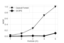
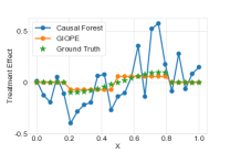
We look at the mean squared error of the treatment effect prediction on 25 equally spaced points in $[0,1]$. Figure 1 (a) compares the MSE between our method with causal forest (CF). GIOPE shows smaller MSE and as the horizon increases the benefit is more apparent. Figure 1 (b) shows the predicted value of the treatment effect for our method and causal forest for horizon $H=4$ along with the true treatment effect for different values of $x$. This illustrates the reason of performance gap. Our method partitions the state space and makes the same prediction for each subgroup that results in more accurate predictions, whereas causal forests over-splits and compute different values of the treatment effect for every value of $x$ which are often inaccurate.

(a)	(b)	(c)	(d)

Figure 1: Toy MDP: (a) Mean squared error of treatment effect prediction for our method and causal forest(CF). (b) True and predicted treatment effect for different values of $x$ for our method and causal forest. Sepsis simulator: comparison with causal forest (CF). (c) Mean squared error of prediction. (d) Average size of the 95% confidence intervals (CI

6.2 Sepsis Simulation

There has been growing number of literature that seek to learn an automated policy to manage septic patients in the ICU, reader may find a short review in  Gottesman et al. (2019). However, newly suggested decision policies may be beneficial for some subgroups of patients while harmful to others. We use the sepsis simulator developed in Oberst and Sontag (2019) to show case this scenario and evaluate our models in detecting such subgroups.

Simulator

In this simulator each patient is described by four vital signs {heart rate, blood pressure, oxygen concentration and glucose level} and a binary indicator of diabetes, that take values in a subset of {very high, high, normal, low, very low}, that results in a state space of size $|S|=1440$. In each step the agent can take an action to put the patient on or off of treatment options, {antibiotics, vasopressors, and mechanical ventilation}, so that the action space has cardinality $|A|=2^{3}$. Each episode run until the horizon $H$ which incurs the reward of -1 upon death, +1 upon discharge and 0 otherwise. We use a discount factor of $\gamma=0.99$ across all experiments, and all reported results are averaged over 15 different runs.

Data Generation

In order to form the behaviour and the evaluation policy we assume both policies act nearly optimal with some modifications. We perform policy iteration to find the (deterministic) optimal policy for this environment and soften the policy by subtracting $0.1$ probability from the optimal action and equally distributing it among other actions, we call this policy $\pi_{st}$. We assume the behaviour policy $\pi_{b}$ is similar to $\pi_{st}$ except it has has $15\%$ less chance of using the mechanical ventilator. On the other hand, the evaluation policy $\pi_{e}$ is similar to $\pi_{st}$ but has $20\%$ less chance of using the vasopressor. Notice that, the evaluation policy utilized the mechanical ventilator more and vassopressor less than the behaviour policy. Regardless of the horizon, the evaluation policy achieves better expected discounted return than the behaviour policy. However, there are subgroups of individuals, for example diabetics, that will worse off by using the evaluation policy. We generate $50000$ trajectories using the behaviour policy.

Comparison

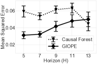
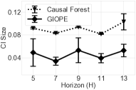
First we look at the mean squared error computed on the individual level. In order to compute this value, for each individual in the test set that consists of $n=20000$ samples from the same distribution as the training set, we sample $30$ different trajectories using the evaluation policy and the behaviour policy to compute the true treatment effect for each individual. Figure 1 shows the mean squared error of prediction made by our method versus causal forest (CF). As shown in Figure 1 (c), our method outperforms the baseline but as horizon increases both models struggles to generate valid results. Panel (d) of Figure 1 shows the average size of the 95% confidence intervals. This highlights one of the main benefits of our method, that is more accurate prediction along with tighter confidence intervals.

Identified Subgroups

Our methods can identify subgroups with significant negative treatment effect, those groups represent patients with diabetes and elevated heart rate. For detailed description of each subgroups for different horizons please refer to supplementary materials. This qualitative analysis unfortunately cannot be done for methods like causal forest as they are not designed to yield distinctive subgroups.

(a)	(b)	(c)	(d)

Figure 2: Ablation study. (a) Mean squared error computed on individual level. (b) Group mean squared error. Coverage: (c) Percentage of groups that the true group treatment effect is covered by the 95% confidence interval. (d) Average size of confidence intervals.

Ablation Study

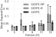
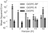
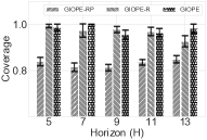
In order to showcase the benefit of each modification that we proposed, we perform ablation study on the sepsis simulator. We compare three different methods with 15 different runs.

1. GIOPE: Using the loss function presented in equation 5.2. In all experiments, the value of regularization is set to $C=5.0$ and the margin $\alpha=0.05$. We found that changing this regularization value has little effect on the results as we presented in the Appendix.

2. GIOPE - Regularization (GIOPE-R): Using the loss function in equation 5 with the suggested proxy variance in equation 7.

3. GIOPE - Regularization and Proxy Variance (GIOPE-RP): This method uses the loss function presented in equation 5 with the sample variance estimate. Note that this basic version is similar to the loss function proposed in Athey and Imbens (2016).

First we look at mean squared error computed on the individual level. As shown in Figure 2 (a) our method shows significant benefits compared to GIOPE-R and GIOPE-RP. This comes with an important observation that our method also shows more stability as the performance does not fluctuates as much across different horizons as well as having smaller standard errors. Note that, our method do not optimize for this objective and the individual mean squared error is best minimized with the sample variance in the limit of infinite data, the benefit comes as an externality of avoiding to predict each individual separately.

Next we look at mean squared error in group treatment effect. That is, for a groups $i$, denote the prediction of the group treatment effect by $\hat{g}_{i}$ and the true group treatment effect by $g_{i}$, then the group MSE is defined as $\frac{1}{G}\sum_{i=1}^{G}(g_{i}-\hat{g}_{i})^{2}$, where $G$ is the total number of groups. Figure 2 (b) shows the MSE in group treatment effect as we increase the horizon. Similar to individual MSE, our method obtains lower MSE and displays more stability across different horizons. This stability is mainly due to avoiding to over split. For example, average number of discovered groups in GIOPE-RP method for horizon 13 is 26 whereas for other GIOPE-R is 5 and GIOPE is 4.

Finally we look at coverage. Figure 2, panel (c) shows the coverage of 95% confidence intervals of the true group treatment effect for different methods and horizons. Methods that use variance proxy instead of sample variance show consistently more coverage. Figure 2 panel (d) shows the average size of the confidence interval for each group treatment effect prediction. This indicates that using the upper bound along with regularization (GIOPE) yields more coverage while offering tighter confidence intervals. This observation highlights the main benefit of using regularization along with proxy variance that allows us to discover groups that we can more accurately and confidently predict their treatment effect. Smaller standard error of confidence intervals size highlights the stability of GIOPE across different runs.

6.3 ICU data - MIMIC III

To show how our method can be used on a real data set, we use a cohort of 14971 septic patients in the freely accessible MIMIC III dataset (Johnson et al., 2016). Prior work Komorowski et al. (2018) used off policy learning and proposed a new decision policy that might provide improved patient outcomes on average. More details on the experiment setup and the off policy learning approach used are in the supplementary materials. Using weighted importance sampling the estimated value of the decision policy is $65.33$ with effective sample size of $146.8$ which suggest an increase of $2.43$ on the survival chance compared to the behaviour policy. Here we take this decision policy and estimate its impact on different potential subgroups.

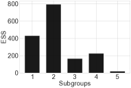
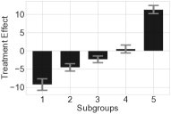
In Figure 3 we present the five groups produced by our algorithm along with their estimated group treatment effect (which is the difference between the baseline clinician policy and the decision policy) and effective sample size of weighted importance sampling in each subgroup. While some of patients fall into subgroup 3, 4 and 5, there are a number of patients that may experience no benefit or even a potential negative treatment effect from the proposed new treatment policy (groups 2 and 1). This highlights how our method may be useful in identifying subgroups in which a new decision policy may be beneficial or harmful relative to the standard approach.

We caveat the results in this section by noting that using IS based methods on real world datasets, and the MIMIC III dataset in particular is very susceptible to noise induced by the small effective sample size of the cohort (Gottesman et al., 2018). Furthermore, our method is susceptible to this source of noise twice, as IS based estimators are used both in the partitioning phase and the estimation phase. However, despite their high susceptibility to noise, IS methods are often applied to the MIMIC III dataset for their theoretical properties, but their results for real data should be interpreted with caution. In our experiment we intentionally designed the decision policy close to the behaviour policy to avoid issues arising from small effective sample size.

(a)	(b)	(c)	(d)

Figure 3: MIMIC III dataset. AI Clinician: Although positive treatment effect is predicted by weighted importance sampling on the full cohort, groups 1 and 2 will like be harmed by the evaluation policy. (a) Estimated treatment effect for each subgroup, (b) Effective sample size of weighted importance sampling for each subgroup. More aggressive vasopressor use: (c) Estimated treatment effect for each subgroup, (d) Effective sample size of weighted importance sampling for each subgroup

More Aggressive Use of Vasopressor

Additionally, we evaluated our method on a policy that utilizes vasopressor more often than the behaviour policy. We estimate the behaviour policy using KNN, and evaluate a policy that has 10% more probability mass on using vasopressor than the behaviour policy. Figure 3 (c) shows the subgroups found using our method along with the effective sample size of every group in display (d).

Group 1, 2, and 3 all show a negative treatment effect. Interestingly, these three groups have SOFA $>1$ which indicates these patients are at high risk. Given the discussions we had with an intensivist, this is in agreement with their expectation that healthier patients are less likely to be harmed by more aggressive use of vasopressor, and sicker patients may be more at risk. This also highlights one of the main benefits of our method: it can be used to provide interpretable subgroups with differing potential treatment effects that may be used to support communication with clinicians around potentially beneficial alternate treatments, and who they might benefit.

7 Conclusion and Future Works

In this paper, we proposed a novel method to partition the feature space, enabling us to find subgroups that we can accurately and confidently predict the group treatment effect for them. Our approach is in contrast with previous methods that estimate individual-level treatment effects, yielding uncertain and less accurate predictions. We do so, by proposing a novel loss function that utilizes; 1. A proxy on the variance estimator that is easy to compute and stable; 2. A regularization term that incentivizes the discovery of groups with significant treatment effect and allows us to integrate domain expert’s input into partitioning algorithm. We further evaluate our method on both simulated domains and real-world data.

Our method can leverage the existing data to raise caution when necessary about a possible negative effect of the newly suggested decision policy on some subgroups. Additionally, results from our method, when applied to observational data, can help to design multi-stage randomized trials that are powered toward detecting harm or benefit of the evaluation policy compared to the baseline policy for specific subgroups. However, it is crucial not to overly rely on the results of our method to justify certain treatments. Most of the findings, especially in health care, have to be validated via a randomized clinical trial or with an extensive discussion with the medical team.

Here, we discuss some limitations and avenues of future works. The current method only employs importance sampling to obtain an estimate of the treatment effect. However, it is well known that the importance sampling method can have high variance. Integrating other methods of off-policy policy evaluation in the partitioning phase, for example doubly robust or model-based method (Thomas and Brunskill, 2016), can mitigate this issue and result in better partitioning.

Additionally, we suggested using recursive partitioning to minimize the loss function; however, these greedy algorithms may fail to find the optimal solution; thus, an immediate question is how can we apply better optimization techniques. Finally, we consider subgroups for the initial state. For example, for septic patients in ICU, this corresponds to their states upon admission. Although, there has been evidence supporting this way of grouping for different sepsis phenotypes (Seymour et al., 2019) an interesting avenue of future research is considering groups based on transition dynamics. For example, patients that react differently to various medications may be part of the same group.

Appendix A Appendix

A.1 Proof

Here we present the proof of the theorem 1. We restate the theorem first.

Theorem (1).

For a given partition $L\in\Pi$, let $T(x;L)$ be the group treatment effect defined in equation 2, $t(x)$ be the individual treatment effect as defined in equation 1 and $\hat{T}(x;L)$ an unbiased estimator of $T(x;L)$. The following display impose the same ranking over the partitions as the MSE loss in equation 4.1:

$$-\mathbb{E}_{x\sim\mathcal{X}}\left[\hat{T}^{2}(x;L)\right]+2~{}\mathbb{E}_{x\sim\mathcal{X}}\left[\mathbb{V}\left[\hat{T}(x;L)\right]\right]$$ (10)

Where $\mathbb{V}[\hat{T}(x;L)]$ is the variance of the estimator $\hat{T}(x;L)$.

Proof.

First, We form the adjusted MSE (AMSE) as

$$AMSE(\hat{T};L)=\underset{x\sim\mathcal{X}}{\mathbb{E}}\left[\left(t(x)-\hat{T}(x;L)\right)^{2}-t(x)^{2}\right]$$

Adjusted MSE and MSE impose the same ranking among different partitioning as $\underset{x\sim\mathcal{X}}{\mathbb{E}}[t(x)^{2}]$ is independent from the partitioning. Note that adjusted MSE, similar to MSE cannot be computed.

We continue by decomposing the adjusted MSE by adding and subtracting $T(x;L)$,

$$AMSE(\hat{T};L) =-\mathbb{E}_{x\sim\mathcal{X}}\left[\left(t(x)-\hat{T}(x;L)\right)^{2}-t(x)^{2}\right]$$

$$=\mathbb{E}_{x\sim\mathcal{X}}[\underbrace{(t(x)-T(x;L))^{2}-t(x)^{2}}_{(i)}$$

$$+\underbrace{(T(x;L)-\hat{T}(x;L))^{2}}_{ii}$$

$$+\underbrace{2(t(x)-T(x;L))(T(x;L)-\hat{T}(x;L))}_{(iii)}]$$

Now we look at each part separately, for part $(i)$,

$$\mathbb{E}_{x\sim\mathcal{X}}\left[(t(x)-T(x;L))^{2}-t(x)^{2}\right]=$$

$$\mathbb{E}_{x\sim\mathcal{X}}\left[T(x;L)^{2}-2t(x)T(x;L)\right]$$

Now we expand the expectation over each group of thr partition $L=\{l_{1},\dots,l_{M}\}$,

$$\sum_{l_{i}\in L}P(l_{i})T(x;l_{i})^{2}-2\sum_{l_{i}\in L}P(l_{i})T(x;l_{i})$$

Where $T(x;l_{i})=T(x;L)$ such that $x\in l_{i}$, note that by definition, $T(x;l_{i})$ is constant for all $x\in l_{i}$. Next, note that $\mathbb{E}_{x\in l_{i}}[t(x)]=T(x;l_{i})$.

$$\sum_{l_{i}\in L} P(l)T(x;l_{i})^{2}-2\sum_{l_{i}\in L}P(l_{i})T(x;l_{i})^{2}=$$

$$-\sum_{l_{i}\in L} P(l_{i})T(x;l_{i})^{2}=-\mathbb{E}_{x\sim\mathbb{X}}[T(x;L)^{2}]$$ (11)

Now, consider the variance of $\hat{T}(x;l_{i})$ for group $l_{i}\in L$,

$$\mathbb{V}\left[\hat{T}(x;l)\right] =\underset{x\in l_{i}}{\mathbb{E}}[\hat{T}^{2}(x;l_{i})]-\left[\underset{x\in l_{i}}{\mathbb{E}}\hat{T}(x;l_{i})\right]^{2}$$

$$=\underset{x\in l_{i}}{\mathbb{E}}[\hat{T}^{2}(x;l_{i})]-T(x;l_{i})^{2}$$ (12)

Which follows by $\hat{T}(x;l_{i})$ being an unbiased estimator of $T(x;l_{i})$. Taking the expectation over the feature space and substituting equation A.1 into A.1,

$$(i) =-\sum_{l_{i}\in L}P(l_{i})T(x;l_{i})^{2}$$

$$=\sum_{l_{i}\in L}P(l_{i})\left[\mathbb{V}\left[\hat{T}(x;l_{i})\right]-\mathbb{E}_{x\sim l_{i}}\left[\hat{T}^{2}(x;l_{i})\right]\right]$$

$$=\mathbb{E}_{x\sim\mathbb{X}}\left[\mathbb{V}\left[\hat{T}(x;l)\right]\right]-\mathbb{E}_{x\sim\mathbb{X}}\left[\hat{T}^{2}(x;l)\right]$$

Now we consider part $(ii)$,

$$\mathbb{E}_{x\sim\mathbb{X}}\left[\left(T(x;L)-\hat{T}(x;L)\right)^{2}\right]$$

$$=\sum_{l_{i}}P(l_{i})\mathbb{E}_{x\in l_{i}}\left[\left(T(x;l_{i})-\hat{T}(x;l_{i})\right)^{2}\right]$$

$$=\sum_{l_{i}}P(l_{i})\mathbb{E}_{x\in l_{i}}\left[\left(\mathbb{E}_{x\in l_{i}}[\hat{T}(x;l_{i})]-\hat{T}(x;l_{i})\right)^{2}\right]$$

$$=\sum_{l_{i}}P(l_{i})\mathbb{V}\left[\hat{T}(x;l_{i})\right]$$

$$=\mathbb{E}_{x\sim\mathbb{X}}\left[\mathbb{V}\left[\hat{T}(x;L)\right]\right]$$

Where the third line follows by $\hat{T}(x;l_{i})$ being an unbiased estimator of $T(x;l_{i})$.

Looking at the last term $(iii)$,

$$\mathbb{E}_{x\sim\mathcal{X}}\left[\left(t(x)\hat{T}(x;L)\right)\right] =\sum_{l_{i}\in L}P(l_{i})\mathbb{E}_{x\in l_{i}}\left[t(x)\hat{T}(x;l_{i})\right]$$

$$=\sum_{l_{i}\in L}P(l_{i})\hat{T}(x;l_{i})\mathbb{E}_{x\in l_{i}}\left[t(x)\right]$$

$$=\sum_{l_{i}\in L}P(l_{i})\hat{T}(x;l_{i})T(x;l_{i})$$

$$=\mathbb{E}_{x\in\mathcal{X}}\left[\hat{T}(x;l_{i})T(x;l_{i})\right]$$

Which implies $\mathbb{E}_{x\sim\mathcal{X}}\left[(t(x)-T(x;L))\hat{T}(x;L)\right]=0$. As a result,

$$(iii) =2\mathbb{E}_{x\in\mathcal{X}}\left[\left(t(x)-T(x;L)\right)\left(T(x;L)-\hat{T}(x;L)\right)\right]$$

$$=2\mathbb{E}_{x\in\mathcal{X}}\left[\left(t(x)-T(x;L)\right)\left(T(x;L)\right)\right]$$

$$-2\mathbb{E}_{x\in\mathcal{X}}\left[\left(t(x)-T(x;L)\right)\left(\hat{T}(x;L)\right)\right]=0$$

Putting the results together, results in equation 5.2. ∎

Next, we continue with the proof of Theorem 2. First, we present a reminder on Rényi divergence.

Rényi Divergence

For $\alpha\geq 0$ the Rényi divergence for two distribution $P$ and $Q$ as defined by [Cortes et al., 2010] is

$$D_{\alpha}(P||Q)=\frac{1}{\alpha-1}\log_{2}\sum_{x}Q(x)\left(\frac{P(x)}{Q(x)}\right)^{\alpha-1}.$$

Denote the exponential in base 2 by $d_{\alpha}(P_{e}||P_{b})=2^{D_{\alpha}(P_{e}||P_{b})}$.

The effective sample size (ESS) [Kong, 1992] is often used for diagnosis of IS estimators, and is defined as

$$ESS(P||Q)=\frac{N}{1+\mathbb{V}_{x\sim Q}[w(x)]}=\frac{N}{d_{2}(P||Q)}$$

where $N$ is the number of samples drawn to estimate the importance weights. A common estimator of the ESSOwen [2013] is

$$\widehat{ESS}(P||Q)=\frac{\left(\sum_{i=1}^{N}w_{i}\right)^{2}}{\sum_{i=1}^{N}w_{i}^{2}}$$

Theorem (2).

Given a dataset $\mathcal{D}=\{(x_{0},\rho_{0},g_{0}),\dots,(x_{N},\rho_{N},g_{N})\}$ and the treatment effect estimator defined by $\hat{T}=\frac{1}{N}\sum_{i}(\rho_{i}-1)g_{i}$. The variance of $\hat{T}$ satisfies the following inequality,

$$\mathbb{V}[\hat{T}]\leq\left\lVert g\right\lVert^{2}_{\infty}\left(\frac{1}{ESS}-\frac{1}{N}\right)$$ (13)

where, $ESS$ is the effective sample size.

Proof.

First note that the variance of the treatment effect estimator $\hat{T}=\frac{1}{N}\sum_{i}(\rho_{i}-1)g_{i}$ can be upper bounded by the variance of the importance sampling weights. Since $\mathbb{V}[\hat{T}]\leq\mathbb{E}[\hat{T}^{2}]$

$$\mathbb{V}[\hat{T}]\leq\frac{||g||^{2}_{\infty}}{N^{2}}\mathbb{E}\left[\sum_{i}(\rho_{i}-1)^{2}\right]=\frac{1}{N}||g||^{2}_{\infty}\mathbb{V}[\rho],$$

where the last equality follows by observing that $\mathbb{E}[\rho]=1$. As noted by Metelli et al. [2018], The variance of the treatment effect estimator can be written as

$$\mathbb{V}[\hat{T}]\leq\||g||^{2}_{\infty}(\frac{d_{2}(P_{e}||P_{b})}{N}-\frac{1}{N})$$

This expression can be related to the effective sample size of the original dataset given the evaluation policy, resulting in equation 13

$$\mathbb{V}[\hat{T}]\leq||g||^{2}_{\infty}\left(\frac{1}{ESS}-\frac{1}{N}\right)$$

∎

Appendix B Experimental Details

In this section we present details of the experimental setups along with some extra experiments that shows the effect of the regularization on the results reported in the main text.

B.1 Simple Illustration

We consider a simple Markov decision process (MDP) with the state space $x\in[0,1]$, discrete action space $a\in\{-1,0,1\}$ and the reward function is defined as $r(x)=1-|x-0.5|$. The transition dynamic is specified by, $x_{t+1}=clip(x_{t}+\kappa\times a_{t}+\epsilon,0,1)$, where the function $clip(x,a,b)$, clips the value of $x$ between $a$ and $b$, $\kappa=0.2$ and $\epsilon\sim\mathcal{N}(0,0.05)$. Each episode lasts $H$ steps. Intuitively, action $1$ takes the agent to the right, $-1$ to the left and $0$ same location with some gaussian noise. If the agent hits the boundary, the action has no effect on the position.

The behaviour policy, takes action with the following probabilities

$$\left\{\begin{aligned} x<0.2:~{}&\pi_{b}(-1)=0.25,~{}\pi_{b}(0)=0.25,~{}\pi_{b}(1)=0.5\\ x\geq 0.2:~{}&\pi_{b}(-1)=0.5,~{}\pi_{b}(0)=0.25,~{}\pi_{b}(1)=0.25\\ \end{aligned}\right.$$

And the evaluation policy,

$$\left\{\begin{aligned} x>0.8:~{}&\pi_{e}(-1)=0.5,~{}\pi_{e}(0)=0.25,~{}\pi_{e}(1)=0.25\\ x\leq 0.8:~{}&\pi_{e}(-1)=0.25,~{}\pi_{e}(0)=0.25,~{}\pi_{e}(1)=0.5\\ \end{aligned}\right.$$

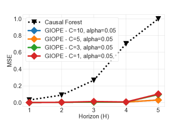
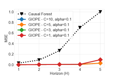
We generated $50000$ trajectories with the behaviour policy for horizons $\{1,2,3,4,5\}$ and averaged all results over 10 runs. Figure 4 compares the mean squared error of our method versus the causal forests for different range of hyper-parameters. Panel (a) shows the results for margin $\alpha=0.05$ and values of regularization constant $C=\{1,3,5,10\}$ and panel (b) shows the results for margin $\alpha=0.1$. As shown, regularization has small effects on the results and the results reported in the main text holds for a large range of hyper-parameters.

(a) $\alpha=0.05$	(b) $\alpha=0.1$

Figure 4: Toy MDP. (a) regularization margin $\alpha=0.05$, (b) regularization margin $\alpha=0.1$

B.2 Sepsis Simulation

We used the following set of hyper-parameters for the experiments presented in section 6. Regularization constant $C=5.0$, regularization margin $\alpha=0.05$, regularization confidence value $\delta=0.4$, maximum depth of the tree $d=\infty$ and minimum number of samples in each leaf $50$. Figure 5 shows the partitions found in horizon $\{5,9,11\}$. As shown, our method can recover groups with significant negative treatment effect in every horizon.

(a)	(b)	(c)	(d)

Figure 5: Sepsis simulation. Group treatment effect for a sample run with horizon (a) 5, (b) 7, (c) 9 (d) 13

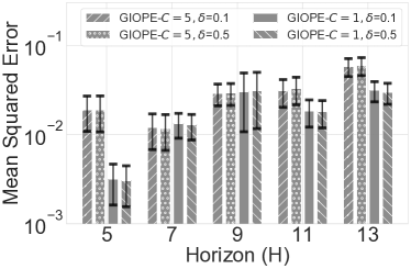
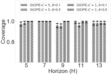
In order to evaluate the effect of hyper-parameters, we perform the ablation study for two different values of regularization confidence interval $\delta=0.1$ and $\delta=0.4$ and two different values of regularization constant $C=5.0$ and $C=1.0$. Figure 6 (a) shows the result for mean squared error and (b) for group mean squared error. As shown, the effect of regularization is small, and the same results as in the main text can be obtained with different range of hyper-parameters. Similarly, figure 6 (c) shows the coverage of the 95% confidence interval and (d) is the average size of CI. The results obtained in the main text holds with different value of hyper-parameters.

(a)	(b)
(c)	(d)

Figure 6: Ablation study, results of GIOPE for four different values of parameters. (a) Mean squared error (b) group mean squared error, (c) 95% confidence interval coverage and (d) average size of confidence intervals

B.3 MIMIC-III

We used MIMIC-III dataset [Johnson et al., 2016], and following Komorowski et al. [2018] extracted the sepsis cohort. Our training set consist of 14971 individuals, with 8442 male and 6529 female. The mortality rate in our cohort is 18.4%. The feature space is of size 44 consist of the following values:

{gender, re_admission, mechvent, age, Weight_kg, GCS, HR, SysBP, MeanBP, DiaBP, RR, Temp_C, FiO2_1, Potassium, Sodium, Chloride, Glucose, Magnesium, Calcium, Hb, WBC_count, Platelets_count, PTT, PT, Arterial_pH, paO2, paCO2, Arterial_BE, Arterial_lactate, HCO3, Shock_Index, Shock_Index, PaO2_FiO2, cumulated_balance, SOFA, SIRS, SpO2, BUN, Creatinine, SGOT, SGPT, Total_bili, INR, output_total, output_4hourly}

We provide the index of the patients in the dataset to facilitate reproducibility of our results.

In order to estimate the behaviour policy, we use KNN with $k=100$ on the test set, we use $l_{2}$ distance with uniform weights across different features to measure the distance. If an action was not taken among all 100 nearest neighbours, we assign the probability $0.01$ to the action. We used IV fluid and mechanical ventilation for actions and used $20\%$ quantile to discretize the action space into $25$ actions.

For the evaluation policy, we used a similar method as the behaviour policy on a random subset of training set (20% of the training data). We only used the following features to estimate the distance for the evaluation policy,

{HR, SysBP, Temp_C, Sodium, Chloride, Glucose, Calcium, paO2, Arterial_BE, SOFA, SIRS, Creatinine}

Simiarly, if an action was not taken among all 100 nearest neighbours, we assign the probability $0.01$ to the action. In our experiments in section 6 we used the following set of hyper-parameters: regularization constant $C=100.0$, regularization margin $\alpha=0.0$, regularization confidence value $c=2.0$, maximum depth of the tree $d=\infty$ and minimum number of samples in each leaf $1000$.

References

- Athey and Imbens [2016] Susan Athey and Guido Imbens. Recursive partitioning for heterogeneous causal effects. Proceedings of the National Academy of Sciences, 113(27):7353–7360, 2016.
- Athey et al. [2019] Susan Athey, Julie Tibshirani, Stefan Wager, et al. Generalized random forests. Annals of Statistics, 47(2):1148–1178, 2019.
- Breiman et al. [1984] Leo Breiman, Jerome Friedman, Charles J Stone, and Richard A Olshen. Classification and regression trees. CRC press, 1984.
- Chernozhukov et al. [2018] Victor Chernozhukov, Denis Chetverikov, Mert Demirer, Esther Duflo, Christian Hansen, Whitney Newey, and James Robins. Double/debiased machine learning for treatment and structural parameters, 2018.
- Cortes et al. [2010] Corinna Cortes, Yishay Mansour, and Mehryar Mohri. Learning bounds for importance weighting. In Nips, volume 10, pages 442–450. Citeseer, 2010.
- Craig et al. [2020] Erin Craig, Donald A Redelmeier, and Robert J Tibshirani. Finding and assessing treatment effect sweet spots in clinical trial data. arXiv preprint arXiv:2011.10157, 2020.
- Dudík et al. [2011] Miroslav Dudík, John Langford, and Lihong Li. Doubly robust policy evaluation and learning. arXiv preprint arXiv:1103.4601, 2011.
- Gottesman et al. [2018] Omer Gottesman, Fredrik Johansson, Joshua Meier, Jack Dent, Donghun Lee, Srivatsan Srinivasan, Linying Zhang, Yi Ding, David Wihl, Xuefeng Peng, et al. Evaluating reinforcement learning algorithms in observational health settings. arXiv preprint arXiv:1805.12298, 2018.
- Gottesman et al. [2019] Omer Gottesman, Fredrik Johansson, Matthieu Komorowski, Aldo Faisal, David Sontag, Finale Doshi-Velez, and Leo Anthony Celi. Guidelines for reinforcement learning in healthcare. Nature medicine, 25(1):16–18, 2019.
- Imai and Ratkovic [2014] Kosuke Imai and Marc Ratkovic. Covariate balancing propensity score. Journal of the Royal Statistical Society: Series B: Statistical Methodology, pages 243–263, 2014.
- Jiang and Li [2016] Nan Jiang and Lihong Li. Doubly robust off-policy value evaluation for reinforcement learning. In International Conference on Machine Learning, pages 652–661. PMLR, 2016.
- Johnson et al. [2016] Alistair EW Johnson, Tom J Pollard, Lu Shen, H Lehman Li-Wei, Mengling Feng, Mohammad Ghassemi, Benjamin Moody, Peter Szolovits, Leo Anthony Celi, and Roger G Mark. Mimic-iii, a freely accessible critical care database. Scientific data, 3(1):1–9, 2016.
- Kallus and Uehara [2020] Nathan Kallus and Masatoshi Uehara. Double reinforcement learning for efficient off-policy evaluation in markov decision processes. Journal of Machine Learning Research, 21(167):1–63, 2020.
- Komorowski et al. [2018] Matthieu Komorowski, Leo A Celi, Omar Badawi, Anthony C Gordon, and A Aldo Faisal. The artificial intelligence clinician learns optimal treatment strategies for sepsis in intensive care. Nature medicine, 24(11):1716–1720, 2018.
- Kong [1992] Augustine Kong. A note on importance sampling using standardized weights. University of Chicago, Dept. of Statistics, Tech. Rep, 348, 1992.
- Lee et al. [2020] Hyun-Suk Lee, Yao Zhang, William Zame, Cong Shen, Jang-Won Lee, and Mihaela van der Schaar. Robust recursive partitioning for heterogeneous treatment effects with uncertainty quantification. arXiv preprint arXiv:2006.07917, 2020.
- Liu et al. [2018] Yao Liu, Omer Gottesman, Aniruddh Raghu, Matthieu Komorowski, Aldo Faisal, Finale Doshi-Velez, and Emma Brunskill. Representation balancing mdps for off-policy policy evaluation. arXiv preprint arXiv:1805.09044, 2018.
- Metelli et al. [2018] Alberto Maria Metelli, Matteo Papini, Francesco Faccio, and Marcello Restelli. Policy optimization via importance sampling. 2018.
- Nie and Wager [2017] Xinkun Nie and Stefan Wager. Quasi-oracle estimation of heterogeneous treatment effects. arXiv preprint arXiv:1712.04912, 2017.
- Obermeyer and Emanuel [2016] Ziad Obermeyer and Ezekiel J Emanuel. Predicting the future—big data, machine learning, and clinical medicine. The New England journal of medicine, 375(13):1216, 2016.
- Oberst and Sontag [2019] Michael Oberst and David Sontag. Counterfactual off-policy evaluation with gumbel-max structural causal models. In International Conference on Machine Learning, pages 4881–4890. PMLR, 2019.
- Owen [2013] Art B. Owen. Monte Carlo theory, methods and examples. 2013.
- Precup [2000] Doina Precup. Eligibility traces for off-policy policy evaluation. Computer Science Department Faculty Publication Series, page 80, 2000.
- Seymour et al. [2019] Christopher W Seymour, Jason N Kennedy, Shu Wang, Chung-Chou H Chang, Corrine F Elliott, Zhongying Xu, Scott Berry, Gilles Clermont, Gregory Cooper, Hernando Gomez, et al. Derivation, validation, and potential treatment implications of novel clinical phenotypes for sepsis. Jama, 321(20):2003–2017, 2019.
- Shalit et al. [2017] Uri Shalit, Fredrik D Johansson, and David Sontag. Estimating individual treatment effect: generalization bounds and algorithms. In International Conference on Machine Learning, pages 3076–3085. PMLR, 2017.
- Thomas and Brunskill [2016] Philip Thomas and Emma Brunskill. Data-efficient off-policy policy evaluation for reinforcement learning. In International Conference on Machine Learning, pages 2139–2148. PMLR, 2016.