Supplementary Material
It’s About Time: Analog Clock Reading in the Wild

Appendix A Digital Clock Reading

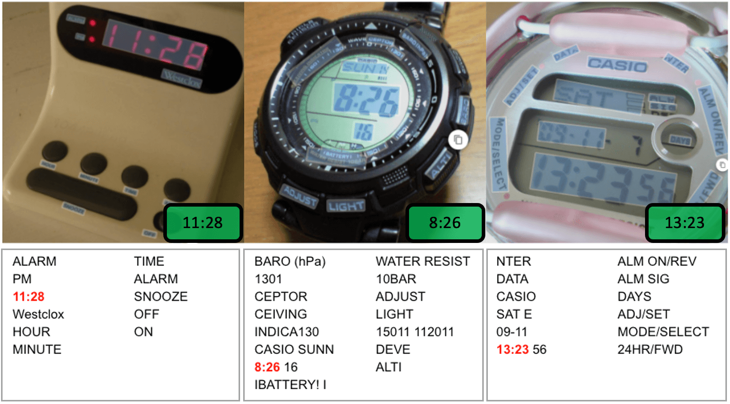
While this paper focuses on reading analog clocks, we also show that digital clocks can simply be read using off-the-shelf optical character recognition (OCR) models in Figure 1. We utilise the cue that hour and minute are usually separated by a colon (:) in extracting text.

While this method allows clock reading in general, it is not very robust as it relies on the presence of the colon, which does not apply to all clocks. Future work can look into combining this with a detection bounding box and ensuring that the number falls into a certain range.

Figure 1: Reading digital clocks. Digital clocks can be read using off-the-shelf text spotting models. The image shows examples of digital clocks, and the text extracted.

Appendix B Homography Warping

In the alignment stage, we learn a homography matrix $\mathcal{\hat{H}}$ with 8 degrees of freedom and use that to warp the image. Projective warping with a homography is governed by the sampling equation:

$$\operatorname{dst}(x,y)=\operatorname{src}\left(\frac{\mathcal{\hat{H}}_{11}^{-1}x+\mathcal{\hat{H}}_{12}^{-1}y+\mathcal{\hat{H}}_{13}^{-1}}{\mathcal{\hat{H}}_{31}^{-1}x+\mathcal{\hat{H}}_{32}^{-1}y+\mathcal{\hat{H}}_{33}^{-1}},\frac{\mathcal{\hat{H}}_{21}^{-1}x+\mathcal{\hat{H}}_{22}^{-1}y+\mathcal{\hat{H}}_{23}^{-1}}{\mathcal{\hat{H}}_{31}^{-1}x+\mathcal{\hat{H}}_{32}^{-1}y+\mathcal{\hat{H}}_{33}^{-1}}\right)$$

One problem is that the homography matrix in the original image coordinates has a large range of values, making the regression difficult to optimise. To normalise them to a similar range, we first scale and translate the image into a [-1, 1] grid and then warp from there, before transforming back to the original space.

In implementation, this is done by transforming the predicted homography itself before warping:

$$\mathcal{\hat{H}}=\begin{bmatrix}s&0&st\\ 0&s&st\\ 0&0&1\end{bmatrix}\mathcal{\hat{H}}\begin{bmatrix}1/s&0&-t\\ 0&1/s&-t\\ 0&0&1\end{bmatrix}$$

where the scale $s$ is equal to half the image size (224/2), and the translation $t$ is 1. This is equivalent to first scaling a 224 $\times$ 224 image to a 2$\times$2, and then translating by -1 on each axis, so that the resultant image falls into a [-1,1] grid.

Appendix C Comparison of Losses

Intuitively, this time reading on analog clocks is more naturally one of regression rather than classification. However, empirically we find otherwise, as indicated by the comparisons in Table 1. In experiments A-D, we compare classification with different variants of regression losses (L1, L1 with separate hour and minute loss, L2). All the regression models fail to train on SynClock, as indicated by the low training accuracy. We then investigated a simpler case in experiments E-F, by removing augmentation, homography and artefacts while training on SynClock. The regression model (model F) can now learn better, but still its generalization to the test data is significantly worse than the classification one. Overall, we observe that classification is easier to train, and gets better performance. We think this is because regression hinders precision, as there is too little penalty for slightly wrong cases, and is hence not suitable for fine-grained recognition in our task.

Model	Aug.	Loss	Train (H/M)	1	1-H	1-M
A	$\checkmark$	cls	94.9/95.5	59.6	71.3	67.0
B	$\checkmark$	reg, L1	73.0/9.6	5.4	49.1	7.3
C	$\checkmark$	reg L2	60.8/6.4	3.2	30.5	5.8
D	$\checkmark$	reg, L1, sep	66.7/7.5	4.2	48.2	6.2
E	✗	cls	98.1/99.7	12.2	25.9	27.1
F	✗	reg, L1	96.1/67.6	3.5	21.5	7.6

Table 1: Comparison between losses. We report the train and test accuracy for different losses. The model is trained on SynClock, and tested on COCO (IOU$>$50).

Appendix D Comparison with Previous Methods

In this section, we compare our results to a geometry-based method using Sobel edge detection and Hough transform [clockreader]. In Table 2, we use the same detection as in our model together with the line/edge based method for recognition. As expected, the model struggles with variations in design, resolution, lighting and artefacts.

Method	COCO	OpenImages	Clock Movies
Geometry based [clockreader]	9.7	7.7	8.2
Ours	80.4	77.3	79.0

Table 2: Comparison with geometry-based methods. We report the Top-1 accuracy on three benchmarks.

Appendix E Broader Social Impact

As this is a new application task in computer vision, we think it is timely to also discuss the broader social impact of our work. As clocks appear in images as the background, sometimes without the subject being aware of it, it may raise privacy concerns given that it gives out more information than what is intended. Moreover, as the application progresses, there may be a possibility of combining this information with other cues such as illumination, where then it is possible to predict where and when the image is taken, raising privacy concerns.

Appendix F Limitations

As introduced in the main paper, the main limitation of our model is its inability to logically reason to the level that human does, such as using the cue of relative position of hands relative to the hour mark. Our model is also unable to generalise well to clocks with unique artistic designs, where humans would understand despite not having seen one before. This includes the example in Figure 6, where the model does not ‘understand’ that the ’hand’ of the cartoon character corresponds to the clock hand. The inability to generalise extends to unique clocks such as backward clocks, and 24-hour clocks.

Appendix G A Note on RANSAC

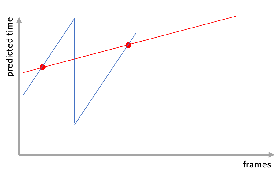
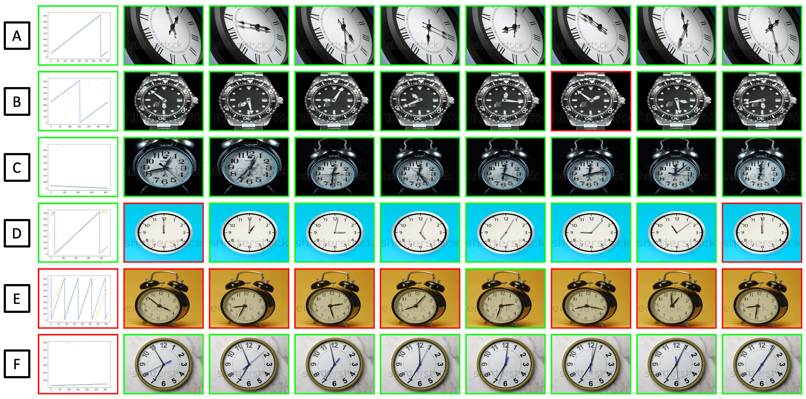
Normally in RANSAC, one would select the minimum number of points that fully parametrises the fit, e.g. 2 for a line, 3 for a quadratic, etc. In the case of a sawtooth wave, having two points is ambiguous, as shown in Figure 3, as it does not know whether the point belongs to the same period, the next one, or whether there are some periods apart, leading to infinitely many solutions. To prevent aliasing, one has to sample above the Nyquist frequency, i.e. the minimum number of points must be more than 2n, where n is the number of periods. This is highly impractical as we do not know n, and sampling that many points especially given a conservative estimate of n is very prone to errors.

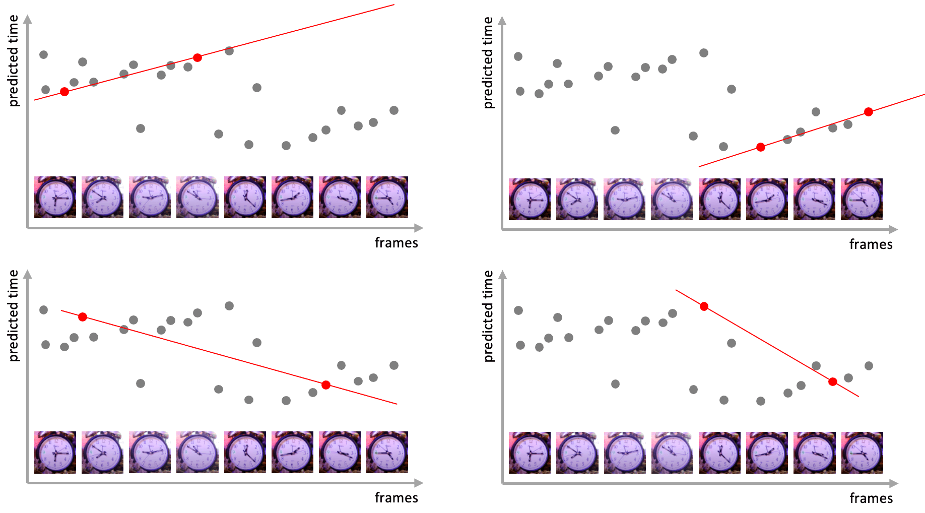
Instead, we opt for a simpler solution, which is to assume that the two points sampled always belong to the same period, and apply rectification afterwards. An immediate disadvantage is that some samples are just useless, such as those in the bottom row of Figure 2. However, there is approximately a 1/n chance that this assumption is valid, and this experimentally allows a good solution to be found given sufficient number of iterations, as in the top row of Figure 2.

While there are other heuristics that can be incorporated, such as sampling neighbouring points more frequently or assuming that time always flows forwards, we find that this simple solution is elegant and sufficient for our use.

Figure 2: A note on fitting a sawtooth wave with RANSAC. The bottom two examples are completely invalid as they violate the assumption that the points belong to the same period. Given a sufficiently large number of iterations this is not a problem.

Figure 3: A note on fitting a sawtooth wave with RANSAC. Given 2 points it is impossible to tell how the sawtooth wave will look like.

Appendix H More examples of RANSAC fitting

Figure 4 shows more examples of video filtering using uniformity constraints. While most videos are correctly filtered, there is some uncommon false positive cases, such as when the clock stops or moves at a different speed towards the start or the end. Accepting part of such videos will be an interesting direction for future work.

Figure 4: More RANSAC examples. Rows A, B and C show examples of correctly filtered videos. Interestingly, the clock in row C flows backwards, but since each individual frame still reads the time correctly, the video is still correctly accepted. Row D shows a false positive case, where the clock is static at the beginning and the end of the video, but is still wrongly accepted to the dataset as the inlier proportion is above the threshold. Row E shows an example where the clock moves uniformly, but RANSAC fails to fit a line within the iteration limit. Therefore the clock is not included in the pseudo-labelled training set even though it qualifies. Row F shows a clock where we exclude from the training set because time moves too slowly, giving not many variations in time, despite being able to fit a line through.

Appendix I More SynClock Examples

We show more examples of images generated from SynClock in Figure 5, varying one parameter at a time.

Figure 5: SynClock examples. From top to bottom row, we show variations in background colour, clock face and shape, clock ticks, numerals, clock hands, artefacts, and homography warping.

Appendix J More Qualitative Results

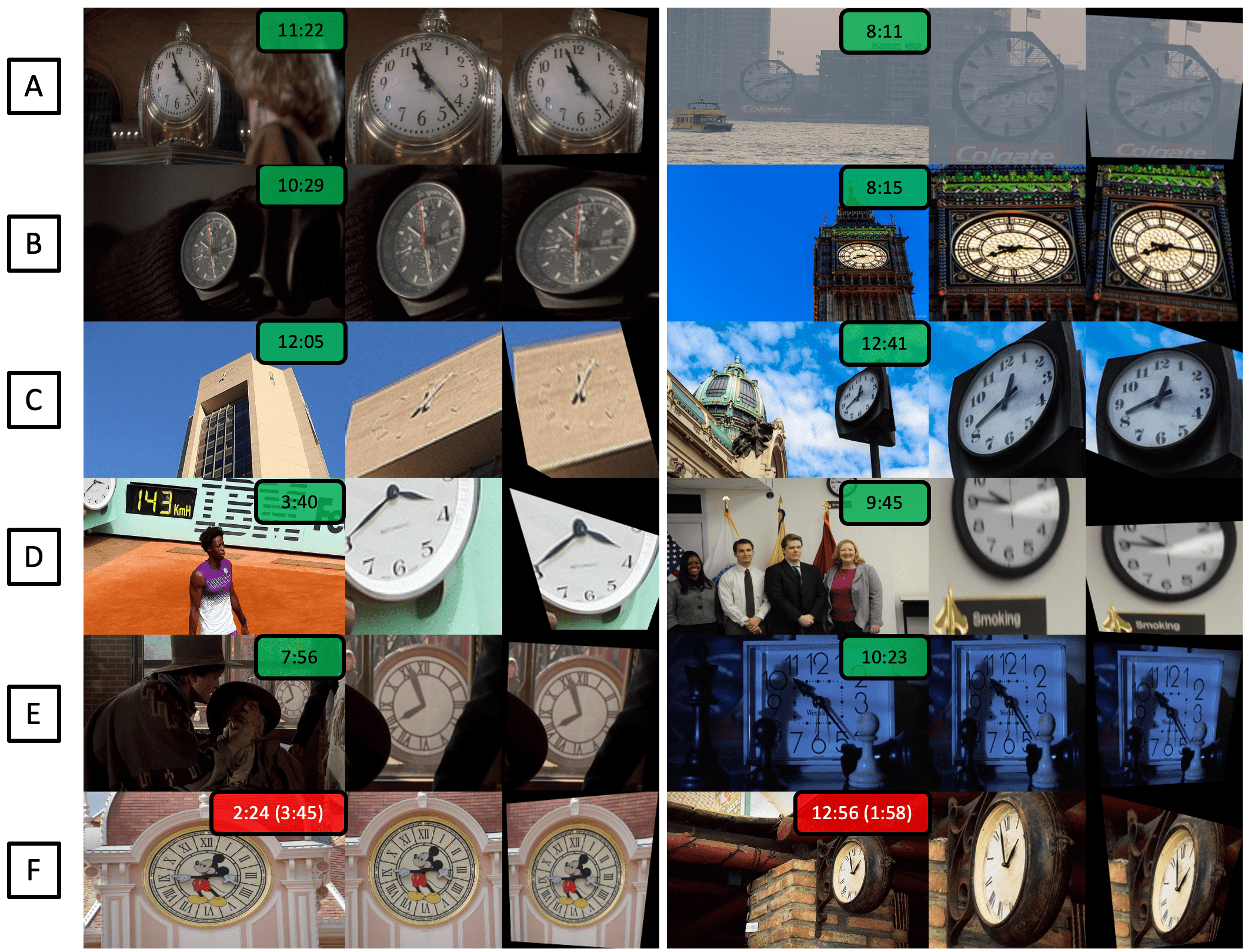
We show more qualitative results in Figure 6.

Figure 6: More Qualitative Results. The columns show the original image, the cropped image with 20% context, and the canonical image. The predicted time reading is overlaid on the original image. We show that the model is able to robustly read clocks with different styles (row A), angles (rows B-C) and occlusion (rows D-E). In the last row (row F), we show a clock style that the model fails to read (left), and a case of too extreme angle (right).