11institutetext: Department of Physics, Indian Institute of Technology, Kanpur-208016, India.22institutetext: CERN, Theoretical Physics Department, CH-1211 Geneva 23, Switzerland.33institutetext: Institute for Particle Physics Phenomenology, Department of Physics, Durham University, Durham DH1 3LE, U.K.44institutetext: Department of Physics, Bangabasi Evening College, 19 Rajkumar Chakraborty Sarani, Kolkata 700009, West Bengal, India.55institutetext: School of Physics & Astronomy, University of Glasgow, Glasgow G12 8QQ, United Kingdom66institutetext: CAFPE and Departamento de Física Teórica y del Cosmos, Universidad de Granada, Campus de Fuentenueva, E–18071 Granada, Spain

Effective limits on single scalar extensions in the light of recent LHC data

Anisha 1,6    Supratim Das Bakshi 2    Shankha Banerjee 3    Anke Biekötter 1    Joydeep Chakrabortty 4    Sunando Kumar Patra 3    Michael Spannowsky   
anisha@glasgow.ac.uk, sdb@ugr.es, shankha.banerjee@cern.ch, anke.biekoetter@durham.ac.uk, joydeep@iitk.ac.in, sunando.patra@gmail.com, michael.spannowsky@durham.ac.uk
Abstract

In this paper, we work with 16 different single scalar particle extensions of the Standard Model. We present the sets of dimension-6 effective operators and the associated Wilson coefficients as functions of model parameters after integrating out the heavy scalars up to 1-loop, including the heavy-light mixing, for each such scenario. Using the correspondence between the effective operators and the observables at electroweak scale, and employing Bayesian statistics, we compute the allowed ranges of new physics parameters that are further translated and depicted in 2-dimensional Wilson coefficient space in the light of the latest CMS and ATLAS data up to 137 fb1137superscript fb1137\text{ fb}^{-1} and 139 fb1139superscript fb1139\text{ fb}^{-1}, respectively. We also adjudge the status of those new physics extensions that offer similar sets of relevant effective operators. In addition, we provide a model-independent fit of 232323 Standard Model effective field theory Wilson coefficients using electroweak precision observables, single and di-Higgs data as well as kinematic distributions of di-boson production.

preprint: CERN-TH-2021-190, IPPP/21/48

1 Introduction

Despite the successful journey of the Standard Model of particle physics (SM), its inadequacy to explain many experimental observations and also the lack of direct evidence of new physics beyond the SM (BSM) in the high energy experiments compel us to look for indirect signatures of new physics (NP). Low-energy observables, such as the electroweak precision observables (EWPOs), the measurement of SM Higgs production and decay modes as well as di-boson production ALEPH:2005ab ; Berthier:2016tkq ; Khachatryan:2016vau ; Aad:2015gba ; Aad:2020plj ; Aad:2020xfq ; ATLAS-CONF-2021-044 ; ATLAS:2020bhl ; ATLAS:2020syy ; ATLAS:2020naq ; ATLAS:2021upe ; CMS:2020gsy ; CMS:2020dvg ; CMS:2020xwi ; CMS:2020mpn ; CMS:2021ixs ; CMS:2020dvp ; CMS:2021kom ; CMS:2021ugl ; Aaboud:2019gxl ; ATLAS:2020nzk ; ATLAS:2019rob ; ATLAS:2018dpp ; ATLAS:2018rnh ; ATLAS:2018uni ; CMS:2020tkr ; CMS:2021ssj ; CMS:2017hea ; Buchmuller:1985jz ; Giudice:2007fh ; Grzadkowski:2010es ; Gupta:2011be ; Gupta:2012mi ; Banerjee:2012xc ; Gupta:2012fy ; Banerjee:2013apa ; Gupta:2013zza ; Elias-Miro:2013eta ; Contino:2013kra ; Falkowski:2014tna ; Englert:2014cva ; Gupta:2014rxa ; Amar:2014fpa ; Buschmann:2014sia ; Craig:2014una ; Ellis:2014dva ; Ellis:2014jta ; Banerjee:2015bla ; Englert:2015hrx ; Ghosh:2015gpa ; Degrande:2016dqg ; Cohen:2016bsd ; Ge:2016zro ; Contino:2016jqw ; Biekotter:2016ecg ; deBlas:2016ojx ; Denizli:2017pyu ; Barklow:2017suo ; Brivio:2017vri ; Barklow:2017awn ; Khanpour:2017cfq ; Englert:2017aqb ; Panico:2017frx ; Franceschini:2017xkh ; Banerjee:2018bio ; Grojean:2018dqj ; Biekotter:2018rhp ; Goncalves:2018ptp ; Gomez-Ambrosio:2018pnl ; Freitas:2019hbk ; Banerjee:2019pks ; Banerjee:2019twi ; Biekotter:2020flu ; Araz:2020zyh ; Ellis:2020unq ; Banerjee:2020vtm ; Almeida:2021asy ; Chatterjee:2021nms , play a crucial role in constraining the SM and leave little room for BSM physics. To understand the present status of NP under the lamp post of experimental data in terms of the non-SM parameters, we need to establish an effective connection between the BSM physics residing at a relatively high scale and observables at the electroweak scale. Effective Field Theories (EFTs) are considered to be elegant tools to extract indirect effects of NP from the experimental data, if any, by bridging the gap between scales.

In a bottom-up approach, the complete and independent set of effective operators for any given mass dimension is computed relying on the symmetry and particle content of the SM – leading to the most popular notion of the Standard Model Effective Field Theory (SMEFT) Grzadkowski:2010es ; BUCHMULLER1986621 ; Brivio_2019 . At dimension six, the commonly used bases of the SMEFT operators include the Warsaw basis 111The Warsaw basis accommodates a set of complete and non-redundant effective operators of mass dimension six.Grzadkowski:2010es ; BUCHMULLER1986621 and the SILH basis Giudice:2007fh ; Elias-Miro:2013mua . Generally, the associated Wilson coefficients (WCs) are independent and not pertinent to any specific UV theory. Parametrising low-energy observables in terms of these WCs and analysing them in global fits allows us to constrain potential NP in a (rather) model-independent way. Global analyses in the SMEFT framework have been performed for the EWPO Han:2004az , Higgs Corbett:2012ja ; Ellis:2014jta ; Dumont:2013wma ; Corbett:2013pja ; Chang:2013cia ; Elias-Miro:2013mua ; Boos:2013mqa ; Ellis:2014dva , di-boson Panico:2017frx ; Baglio:2018bkm ; Grojean:2018dqj ; Baglio:2019uty ; Azatov:2019xxn , the top sector Buckley:2015lku ; Brivio:2019ius ; Bissmann:2019gfc ; Hartland:2019bjb ; Durieux:2019rbz ; vanBeek:2019evb ; CMS:2020pnn , and for combinations of these sectors Ellis:2014jta ; Contino:2016jqw ; Butter:2016cvz ; Biekoetter:2018ypq ; Ellis:2018gqa ; Ellis:2020unq ; Anisha:2020ggj ; Dawson:2020oco ; Ethier:2021bye . In this work, we consider constraints from EWPO, single and di-Higgs data, as well as distributions from the di-boson production channels.

In a top-down approach, the SMEFT lays the platform to bring different BSM scenarios on the same footing by integrating out heavy non-SM degrees of freedom (DOFs). Each effective operator that emerges in the process is accompanied by a WC which is a function of the model parameters and captures the footprints of NP interactions Henning:2014wua ; Drozd:2015rsp ; Henning:2016lyp ; Ellis:2016enq ; Fuentes-Martin:2016uol ; Zhang:2016pja ; Ellis:2017jns ; de_Blas_2018 ; Bakshi:2018ics ; Kramer:2019fwz ; DasBakshi:2020ejz ; DasBakshi:2020pbf ; Haisch_2020 ; Dawson:2021jcl ; Dittmaier:2021fls ; Brivio:2021alv ; Dedes:2021abc . It is important to note that most of the phenomenologically interesting BSM scenarios do not induce the complete set of dimension-6 SMEFT operators. In addition, the Wilson coefficients of effective operators computed by integrating out heavy DOFs from a specific NP Lagrangian are functions of model parameters and thus, unlike the model-independent SMEFT case, they are related to each other. As a result of these relations and the typically smaller number of free parameters, the SMEFT parameter space in a top-down analysis is usually much more stringently constrained compared to bottom-up analyses. Top-down SMEFT fits hence play a crucial role in pinning down the nature of BSM physics.

The primary motivation of this work is to estimate the allowed BSM parameter space for different SM extensions and to perform a comparative analysis among those scenarios that are degenerate effective theories upon non-SM DOFs being integrated out. In our analysis, we consider 16 different single scalar extensions of the SM without extending the gauge symmetry. We embed each of the NP Lagrangians in our Mathematica®®{}^{\text{\tiny\textregistered}} program CoDEx Bakshi:2018ics to perform the integration up to 1-loop, including the heavy-light mixing, and provide the exhaustive sets of the dimension-6 effective operators in Warsaw basis and their associated WCs as functions of model parameters 222We provide the sets of effective operators in both Warsaw and SILH bases for all these BSM scenarios in a Mathematica notebook file here \faGithub.. The effective operators generated for these individual models can be verified using the complementary diagrammatic method introduced in ref. DasBakshi:2021xbl . We work within the Bayesian framework to draw the statistical inference and parameter estimation using the Mathematica®®{}^{\text{\tiny\textregistered}} package OptEx sunando_patra_2019_3404311 .

In this paper we constrain the SMEFT parameter space in both bottom-up as well as top-down approaches to provide an up-to-date map of the new physics parameter space of scalar extensions of the SM. First, we perform a model-independent SMEFT fit based on the latest CMS and ATLAS data, including many distributions and simplified template cross sections. Second, we choose 16 different heavy scalars that are being used frequently in literature for different phenomenological reasons, e.g., neutrino mass generation, to explain IceCube, LHCb data, etc. Dey:2015eaa ; Pilaftsis:1999qt ; Arhrib:2011uy ; Babu:2009aq ; Bambhaniya:2013yca ; Buchmuller:1986zs ; Arnold:2013cva ; Bauer:2015knc ; Bandyopadhyay:2016oif ; Davidson_2010 ; Chen:2008hh . For simplicity, we assume that SM is extended by a single heavy scalar at a time. We compute the effective dimension-6 operators and the associated WCs by performing the integration out of individual heavy fields up to 1-loop, including heavy-light mixing. These matching results incorporating scalar heavy-light mixing are presented in the Warsaw basis. We also provide the results in SILH basis. The obtained results will be useful even when there are multiple heavy scalars. In that case, there will be additional contributions due to mutual interactions among the heavy fields. We further constrain the non-SM parameter space for each individual model using electroweak precision data and Higgs data. We highlight the impact of the individual data sets and their cumulative impact. This helps us to identify which data sets play a crucial role for which model while constraining the non-SM parameter space. We also pin-point the directions in non-SM parameter space that cannot be constrained by our chosen set of data and comment on the observables necessary to constrain these models completely.

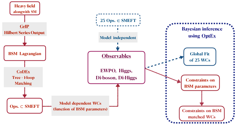
The paper is organised as follows: We provide details on the SMEFT parametrisation of the used observables in section 2 and describe the corresponding experimental inputs in section 3. In section 4, we perform a model-independent analysis including 23 WCs contributing to the EWPO, single Higgs, di-Higgs, and di-boson sectors, and present the results for individual one-parameter fits as well as for a global analysis. In section 5, we introduce the 16 single scalar extensions of the SM and reduce them into effective theories \subset SMEFT. For each case, we tabulate the sets of emerged effective operators and associated WCs in the Warsaw basis as functions of the model parameters. We then employ similar fitting methodology for our chosen two NP models and display the results in terms of model parameters as well as in terms of the WCs, in section 5. We discuss the Renormalisation Group Equations (RGEs) of the SMEFT operators for a specific model and captures its impact on the allowed BSM parameters and WCs in section 6. We summarise our results and discuss possible future directions in section 7. In the appendix B, we tabulate the computed effective operators and the WCs for the remaining 14 models adopted in this work. The working principle of this work is depicted in a flowchart, see fig. 1.
Refer to caption
Figure 1: Flowchart depicting the work-flow of this article. Details on the observables are discussed in section 3. The global fit consists of 23 WCs, see fig. 3. The constraints on the BSM parameters of specific models are discussed in section 5 and appendix B. We use the Hilbert series output from GrIP Banerjee:2020bym to construct the BSM Lagrangian given the heavy field information. The BSM Lagrangians are then implemented in CoDEx Bakshi:2018ics to compute the tree- and the 1-loop-level WCs (including the heavy-light mixed WCs). We perform the statistical analysis based on Bayesian inference using the package OptEx sunando_patra_2019_3404311 .

2 SMEFT parametrisation

The SMEFT describes new physics with higher-dimensional (in mass with dimensions \geq 5) operators consisting of only the SM fields and respecting the SM symmetries. The effective Lagrangian is given by

eff=SMd4+SMEFT=SMd4+d=5,i(𝒞i(d)Λd4)Qi(d),subscripteffsuperscriptsubscriptSM𝑑4superscriptsubscriptSMEFTsuperscriptsubscriptSM𝑑4subscript𝑑5subscript𝑖subscriptsuperscript𝒞𝑑𝑖superscriptΛ𝑑4superscriptsubscript𝑄𝑖𝑑\displaystyle\mathcal{L}_{{}_{\text{eff}}}=\mathcal{L}_{{}_{\text{SM}}}^{d\leq 4}+\mathcal{L}_{{}_{\text{SM}}}^{\text{EFT}}=\mathcal{L}_{{}_{\text{SM}}}^{d\leq 4}+\sum\limits_{d=5,...}\sum\limits_{i}\left(\frac{\mathcal{C}^{(d)}_{i}}{\Lambda^{d-4}}\right)Q_{i}^{(d)}\,, (1)

where Qi(d)superscriptsubscript𝑄𝑖𝑑Q_{i}^{(d)} are the effective operators of mass dimension d𝑑d and 𝒞i(d)subscriptsuperscript𝒞𝑑𝑖\mathcal{C}^{(d)}_{i} are the accompanying WCs, respectively. The index i𝑖i runs over the number of independent effective operators. At dimension six, there are 249924992499 independent operators in the most flavour general case. This number reduces to 595959 when assuming minimal flavour violation (MFV) DAmbrosio:2002vsn and real WCs. On the other hand, in a top-down approach, the number of operators is determined by integrating out the heavy BSM fields. In this work, we have confined ourselves to dimension-6 operators in the Warsaw basis Grzadkowski:2010es and parametrise observables up to linear order in the WCs. The renormalisable part of the SM Lagrangian is given for the sake of completeness as

SMd4superscriptsubscriptSM𝑑4\displaystyle\mathcal{L}_{\text{SM}}^{d\leq 4} =14GμνaGa,μν14WμνIWI,μν14BμνBμν+|DμH|2μH2|H|212λHSM|H|4absent14subscriptsuperscript𝐺𝑎𝜇𝜈superscript𝐺𝑎𝜇𝜈14subscriptsuperscript𝑊𝐼𝜇𝜈superscript𝑊𝐼𝜇𝜈14subscript𝐵𝜇𝜈superscript𝐵𝜇𝜈superscriptsubscript𝐷𝜇𝐻2superscriptsubscript𝜇𝐻2superscript𝐻212superscriptsubscript𝜆𝐻SMsuperscript𝐻4\displaystyle=-\frac{1}{4}G^{a}_{\mu\nu}G^{a,{\mu\nu}}-\frac{1}{4}W^{I}_{\mu\nu}W^{I,{\mu\nu}}-\frac{1}{4}B_{\mu\nu}B^{\mu\nu}+|D_{\mu}H|^{2}-\mu_{{}_{H}}^{2}|H|^{2}-\frac{1}{2}\lambda_{H}^{\text{SM}}|H|^{4}
+l¯LilL+q¯LiqL+e¯RieR+u¯RiuR+d¯RidRsubscript¯𝑙𝐿𝑖italic-D̸subscript𝑙𝐿subscript¯𝑞𝐿𝑖italic-D̸subscript𝑞𝐿subscript¯𝑒𝑅𝑖italic-D̸subscript𝑒𝑅subscript¯𝑢𝑅𝑖italic-D̸subscript𝑢𝑅subscript¯𝑑𝑅𝑖italic-D̸subscript𝑑𝑅\displaystyle+\bar{l}_{{}_{L}}i\not{D}\,l_{{}_{L}}+\bar{q}_{{}_{L}}i\not{D}\,q_{{}_{L}}+\bar{e}_{{}_{R}}i\not{D}\,e_{{}_{R}}+\bar{u}_{{}_{R}}\,i\not{D}\,u_{{}_{R}}+\bar{d}_{{}_{R}}\,i\not{D}\,d_{{}_{R}}
{YeSMHe¯RlL+YuSMH~u¯RqL+YdSMHd¯RqL+h.c.},subscriptsuperscript𝑌SM𝑒superscript𝐻subscript¯𝑒𝑅subscript𝑙𝐿subscriptsuperscript𝑌SM𝑢superscript~𝐻subscript¯𝑢𝑅subscript𝑞𝐿subscriptsuperscript𝑌SM𝑑superscript𝐻subscript¯𝑑𝑅subscript𝑞𝐿h.c.\displaystyle-\left\{Y^{\text{SM}}_{e}H^{\dagger}\bar{e}_{{}_{R}}\,l_{{}_{L}}\,+Y^{\text{SM}}_{u}\widetilde{H}^{\dagger}\bar{u}_{{}_{R}}\,q_{{}_{L}}\,+\,Y^{\text{SM}}_{d}H^{\dagger}\bar{d}_{{}_{R}}\,q_{{}_{L}}\,+\,\text{h.c.}\right\}, (2)

where Bμν,WμνI, and Gμνasubscript𝐵𝜇𝜈subscriptsuperscript𝑊𝐼𝜇𝜈 and subscriptsuperscript𝐺𝑎𝜇𝜈B_{\mu\nu},W^{I}_{\mu\nu},\text{ and }G^{a}_{\mu\nu} are the field strength tensors of the SM gauge groups U(1)Y𝑈subscript1𝑌U(1)_{{}_{Y}}, SU(2)L𝑆𝑈subscript2𝐿SU(2)_{{}_{L}}, and SU(3)C𝑆𝑈subscript3𝐶SU(3)_{{}_{C}}, respectively, with a=1,,8𝑎18a=1,\dots,8. The adopted conventions for the quantum numbers of the SM fields are shown in tab. 2. D𝐷D denotes the covariant derivative, Yu,d,eSMsubscriptsuperscript𝑌SM𝑢𝑑𝑒Y^{\text{SM}}_{u,d,e} are the SM Yukawa couplings, and H~=iσ2H~𝐻𝑖superscript𝜎2superscript𝐻\widetilde{H}=i\,\sigma^{2}\,H^{\ast} is the conjugate Higgs field.

Our SMEFT predictions are computed at linear order in the WCs in the electroweak {αEW,GF,mZ}subscript𝛼𝐸𝑊subscript𝐺𝐹subscript𝑚𝑍\{\alpha_{EW},\,G_{F},\,m_{Z}\} input scheme with the following input values

αEW1=127.95,GF=1.6638×10⁵ GeV2,mZ=91.1876 GeV,mH=125.09 GeV,mt=173.2 GeV.\begin{split}&\alpha^{-1}_{\text{EW}}=127.95,\quad G_{F}=1.6638\times 10^{-5}\text{ GeV}^{-2},\\ m_{Z}=&91.1876\text{ GeV},\quad m_{H}=125.09\text{ GeV},\quad m_{t}=173.2\text{ GeV}\,.\end{split} (3)

We generally assume MFV. However, for the dimension-6 operators contributing to the Yukawa couplings, we distinguish between flavours and introduce different WCs for muons 𝒞μHsubscript𝒞𝜇𝐻\mathcal{C}_{\mu H} and tau leptons 𝒞τHsubscript𝒞𝜏𝐻\mathcal{C}_{\tau H}, as well as the charm 𝒞cHsubscript𝒞𝑐𝐻\mathcal{C}_{cH} and top quarks 𝒞tHsubscript𝒞𝑡𝐻\mathcal{C}_{tH}. There is of course no direct measurement of the charm Yukawa coupling apart from the hJ/ψγ𝐽𝜓𝛾h\to J/\psi\gamma searches Perez:2015aoa and in our analysis 𝒞cHsubscript𝒞𝑐𝐻\mathcal{C}_{cH} can be considered as a proxy for a modification of the total Higgs decay width which can be constrained from a global fit of all Higgs signal strengths. It is important to note that with more data we will be able to explore the structure of the SMEFT operators which may not always follow MFV. Refs. Falkowski:2020znk ; Efrati:2015eaa study various such cases where the requirement for MFV is relaxed.

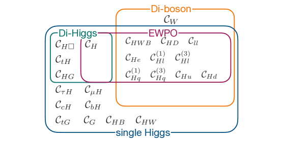
In total, we include 232323 WCs in our model-independent analysis. A graphical summary of the WCs and the observables that they contribute to is given in fig. 2. The corresponding operators are listed in tab. 27 in the appendix E.
Refer to caption
Figure 2: Graphical summary of the considered Wilson coefficients in our model-independent analysis and the observables they contribute to.
Higgs signal strengths and simplified template cross sections:

For the Higgs sector, most of the theory predictions are generated at leading order (LO) using the SMEFTsim model Brivio:2017btx in MadGraph 2.7.3 Alwall:2014hca with the default NNPDF23_NLO parton distribution functions Ball:2013hta . Where available, SMEFT predictions are taken directly from fitmaker Ellis:2020unq , which uses the same tools and settings as outlined above.

For the gluon fusion STXS categories, we instead use the predictions from the ATLAS combination in ref. ATLAS:2020naq which include matching, merging and parton showering. LO predictions for the operator QGsubscript𝑄𝐺Q_{G}, which are not present in the ATLAS reference, are added using the SMEFT@NLO model Degrande:2020evl . For all other channels, we cannot use the ATLAS predictions due to different input parameter scheme choices and instead rely on the predictions at parton level generated with MadGraph. Overall, we describe our Higgs data sets in terms of the following WCs.

𝒞H,𝒞HW,𝒞HB,𝒞HG,𝒞tH,𝒞cH,𝒞bH,𝒞τH,𝒞μH,𝒞G,𝒞tG,𝒞H,𝒞HWB,𝒞HD,𝒞ll,𝒞Hl(1),𝒞Hl(3),𝒞He,𝒞Hq(1),𝒞Hq(3),𝒞Hd,𝒞Hu.\begin{split}\mathcal{C}_{H\square},\quad&\mathcal{C}_{HW},\quad\mathcal{C}_{HB},\quad\mathcal{C}_{HG},\quad\mathcal{C}_{tH},\quad\mathcal{C}_{cH},\quad\mathcal{C}_{bH},\quad\mathcal{C}_{\tau H},\quad\mathcal{C}_{\mu H},\quad\mathcal{C}_{G},\quad\mathcal{C}_{tG},\\ \mathcal{C}_{H},\quad&\mathcal{C}_{HWB},\quad\mathcal{C}_{HD},\quad\mathcal{C}_{ll},\quad\mathcal{C}_{Hl}^{(1)},\quad\mathcal{C}_{Hl}^{(3)},\quad\mathcal{C}_{He},\quad\mathcal{C}_{Hq}^{(1)},\quad\mathcal{C}_{Hq}^{(3)},\quad\mathcal{C}_{Hd},\quad\mathcal{C}_{Hu}.\end{split} (4)

Currently, we only include 𝒞Hsubscript𝒞𝐻\mathcal{C}_{H} in the predictions of total Higgs signal strength measurements and not for STXS measurements. The corresponding contributions of QHsubscript𝑄𝐻Q_{H} to the predictions of different Higgs production and decay channels are used from refs. Degrassi:2016wml ; Degrassi:2019yix . Notice that four-quark operators, which could contribute, for instance, to the tt¯h𝑡¯𝑡t\bar{t}h and th𝑡th categories, are not included in our study at the moment. The inclusion of four-quark operators in global fits with top data has, however, not lead to a weakening of constraints on operators relevant for the top-Higgs sector such as 𝒞tHsubscript𝒞𝑡𝐻\mathcal{C}_{tH}, 𝒞Gsubscript𝒞𝐺\mathcal{C}_{G} and 𝒞HGsubscript𝒞𝐻𝐺\mathcal{C}_{HG} Ellis:2020unq ; Ethier:2021bye . We therefore assume that our approach does not overestimate the constraints on these operators.

Di-Higgs production cross section:

The SMEFT predictions for the di-Higgs production cross section are generated using the ggHH model Heinrich:2020ckp within the POWHEG-BOX-V2 Nason:2004rx ; Frixione:2007vw ; Alioli:2010xd framework which implements BSM effects in a non-linear EFT framework including full NLO QCD corrections with massive top quarks. The Warsaw basis WCs 𝒞isubscript𝒞𝑖\mathcal{C}_{i} are related to the five anomalous couplings cjsubscript𝑐𝑗c_{j} in the ggHH model via

ct=1+v2Λ2𝒞Hv2Λ2yt𝒞tH,ctt=v2Λ2(12𝒞H34yt𝒞tH)chhh=1+3v2Λ2𝒞Hv2λΛ2𝒞H,cggh=2cgghh=(16π)22v2Λ2gs2𝒞HG,\begin{split}c_{t}&=1+\frac{v^{2}}{\Lambda^{2}}\mathcal{C}_{H\square}-\frac{v^{2}}{\Lambda^{2}y_{t}}\mathcal{C}_{tH}\,,\qquad c_{tt}=\frac{v^{2}}{\Lambda^{2}}\left(\frac{1}{2}\mathcal{C}_{H\square}-\frac{3}{4y_{t}}\mathcal{C}_{tH}\right)\\ c_{hhh}&=1+3\frac{v^{2}}{\Lambda^{2}}\mathcal{C}_{H\square}-\frac{v^{2}}{\lambda\Lambda^{2}}\mathcal{C}_{H}\,,\qquad c_{ggh}=2\,c_{gghh}=(16\pi)^{2}\,\frac{2v^{2}}{\Lambda^{2}g_{s}^{2}}\mathcal{C}_{HG}\,,\end{split} (5)

where we use ref. FalkowskiTranlation to translate from the SILH to the Warsaw basis. The effect of the operator QtGsubscript𝑄𝑡𝐺Q_{tG} on the di-Higgs cross section is not taken into account. The di-Higgs cross section is thus parametrised in terms of the operators

𝒞H,𝒞H,𝒞tH,𝒞HG.subscript𝒞𝐻subscript𝒞𝐻subscript𝒞𝑡𝐻subscript𝒞𝐻𝐺\mathcal{C}_{H},\quad\mathcal{C}_{H\square},\quad\mathcal{C}_{tH},\quad\mathcal{C}_{HG}\,. (6)
Di-boson distributions:

We include distributions of WZ𝑊𝑍WZ and WW𝑊𝑊WW production. As shown in ref. Baglio:2019uty , the k𝑘k factors for the SM and the SMEFT interference in di-boson distributions can be very different. The SMEFT predictions for these channels are generated using the WZanomal and WWanomal models Baglio:2019uty within the POWHEG-BOX-V2 which includes NLO QCD corrections Dixon:1999di ; Baur:1994aj ; Azatov:2019xxn . We shower and hadronise our results using Pythia 8.2 Sjostrand:2014zea .

For the WZ𝑊𝑍WZ production with leptonic decays, we include the ATLAS mTWZsuperscriptsubscript𝑚𝑇𝑊𝑍m_{T}^{WZ} production distribution ATLAS:2019bsc . For the last bin of this distribution, which is an overflow bin, we have cut off the SMEFT prediction at mTWZ=1 TeVsuperscriptsubscript𝑚𝑇𝑊𝑍1 TeVm_{T}^{WZ}=1\text{ TeV} to ensure the validity of the EFT. We implement the cuts provided in ref. ATLAS:2019bsc in Rivet Buckley:2010ar and validate the analysis by comparing our POWHEG + Pythia 8.2 SM predictions to the ones in the experimental reference. The SM predictions agree within 5%percent55\,\% in each bin.

For WW𝑊𝑊WW production in the e±νμνsuperscript𝑒plus-or-minus𝜈superscript𝜇minus-or-plus𝜈e^{\pm}\nu\mu^{\mp}\nu final state, we include the leading lepton’s pTsubscript𝑝𝑇p_{T} distribution, pT1superscriptsubscript𝑝𝑇subscript1p_{T}^{\ell_{1}}, from the ATLAS study ATLAS:2019rob . In order to consider the most sensitive bins, we take the predictions of bins 8 to 14. Similar to the WZ𝑊𝑍WZ analysis, we utilise the cuts from the ATLAS study ATLAS:2019rob in Rivet Buckley:2010ar and validate our POWHEG + Pythia 8.2 SM predictions to the ones in the experimental paper. The SM predictions agree within 6%percent66\,\%.

The SMEFT predictions for the ATLAS ΔϕjjΔsubscriptitalic-ϕ𝑗𝑗\Delta\phi_{jj} distribution in the electroweak Zjj𝑍𝑗𝑗Zjj production ATLAS:2020nzk are taken directly from fitmaker. This distribution tightly constrains anomalous triple gauge couplings induced by the operator QWsubscript𝑄𝑊Q_{W}, which is generated in several of the considered SM extensions.

For LEP WW𝑊𝑊WW data, we use the SM and SMEFT parameterisations as well as the theoretical uncertainties from ref. Berthier:2016tkq for the total and differential angular cross-sections at different energies.

The di-boson predictions are expressed in terms of the WCs

𝒞W,𝒞HWB,𝒞HD,𝒞Hl(1),𝒞ll,𝒞Hl(3),𝒞He,𝒞Hq(1),𝒞Hq(3),𝒞Hd,𝒞Hu.subscript𝒞𝑊subscript𝒞𝐻𝑊𝐵subscript𝒞𝐻𝐷superscriptsubscript𝒞𝐻𝑙1subscript𝒞𝑙𝑙superscriptsubscript𝒞𝐻𝑙3subscript𝒞𝐻𝑒superscriptsubscript𝒞𝐻𝑞1superscriptsubscript𝒞𝐻𝑞3subscript𝒞𝐻𝑑subscript𝒞𝐻𝑢\mathcal{C}_{W},\quad\mathcal{C}_{HWB},\quad\mathcal{C}_{HD},\quad\mathcal{C}_{Hl}^{(1)},\quad\mathcal{C}_{ll},\quad\mathcal{C}_{Hl}^{(3)},\quad\mathcal{C}_{He},\quad\mathcal{C}_{Hq}^{(1)},\quad\mathcal{C}_{Hq}^{(3)},\quad\mathcal{C}_{Hd},\quad\mathcal{C}_{Hu}\,. (7)
Electroweak precision observables:

We calculate the SMEFT parametrisations of the EWPO based on refs. Berthier:2015oma ; Brivio:2017vri ; Dawson:2019clf , see also appendix A2 of ref. Anisha:2020ggj for the explicit expressions and tabs. 10.4 and 10.5 of ref. 10.1093/ptep/ptaa104 for the most accurate SM predictions. The EWPO predictions are calculated in terms of the WCs

𝒞HWB,𝒞HD,𝒞ll,𝒞Hl(1),𝒞Hl(3),𝒞He,𝒞Hq(1),𝒞Hq(3),𝒞Hd,𝒞Hu,𝒞H,subscript𝒞𝐻𝑊𝐵subscript𝒞𝐻𝐷subscript𝒞𝑙𝑙superscriptsubscript𝒞𝐻𝑙1superscriptsubscript𝒞𝐻𝑙3subscript𝒞𝐻𝑒superscriptsubscript𝒞𝐻𝑞1superscriptsubscript𝒞𝐻𝑞3subscript𝒞𝐻𝑑subscript𝒞𝐻𝑢subscript𝒞𝐻\mathcal{C}_{HWB},\quad\mathcal{C}_{HD},\quad\mathcal{C}_{ll},\quad\mathcal{C}_{Hl}^{(1)},\quad\mathcal{C}_{Hl}^{(3)},\quad\mathcal{C}_{He},\quad\mathcal{C}_{Hq}^{(1)},\quad\mathcal{C}_{Hq}^{(3)},\quad\mathcal{C}_{Hd},\quad\mathcal{C}_{Hu},\quad\mathcal{C}_{H}\,, (8)

where the contribution of 𝒞Hsubscript𝒞𝐻\mathcal{C}_{H} is only included in the SMEFT parameterisation of mWsubscript𝑚𝑊m_{W} from ref. Degrassi:2021uik .

3 Observables

Our fits include data from EWPO, LEP-WW𝑊𝑊WW measurements as well as LHC data for single Higgs, di-Higgs, di-boson, and electroweak Zjj𝑍𝑗𝑗Zjj production processes.

  • We include a total of 151515 electroweak precision observables. They consist of pseudo-measurements on the Z𝑍Z resonance ALEPH:2005ab , as well as a combination of the W𝑊W mass measurements at LEP ALEPH:2013dgf , Tevatron Group:2012gb and ATLAS ATLAS:2017rzl , the LEP and Tevatron combination of the decay width of the W𝑊W boson Zyla:2020zbs and the Tevatron sin2θeffsuperscript2subscript𝜃eff\sin^{2}\theta_{\text{eff}} measurement CDF:2018cnj

    ΓZ,σhad0,Rl0,Al,Al(SLD),AFBl,Rc0,Ac,AFBc,Rb0,Ab,AFB0,b,mW,ΓW,sin2θeffl(Tev).subscriptΓ𝑍subscriptsuperscript𝜎0hadsubscriptsuperscript𝑅0𝑙subscript𝐴𝑙subscript𝐴𝑙SLDsubscriptsuperscript𝐴𝑙𝐹𝐵subscriptsuperscript𝑅0𝑐subscript𝐴𝑐subscriptsuperscript𝐴𝑐𝐹𝐵subscriptsuperscript𝑅0𝑏subscript𝐴𝑏subscriptsuperscript𝐴0𝑏𝐹𝐵subscript𝑚𝑊subscriptΓ𝑊superscript2superscriptsubscript𝜃eff𝑙Tev\begin{split}\Gamma_{Z},\;\sigma^{0}_{\text{had}},\;R^{0}_{l},\;A_{l},\;&A_{l}(\text{SLD}),\;A^{l}_{FB},\;R^{0}_{c},\;A_{c},\;A^{c}_{FB},\;R^{0}_{b},A_{b},\;A^{0,b}_{FB},\\ &m_{W},\;\Gamma_{W},\;\sin^{2}\theta_{\text{eff}}^{l}(\text{Tev})\,.\end{split} (9)
  • We include LHC single-Higgs data from ATLAS and CMS. For LHC Run I, we incorporate the combination of ATLAS and CMS results in ref. Khachatryan:2016vau . For ATLAS Run II, we add the STXS results from refs. ATLAS:2020naq ; ATLAS:2021upe as well as the measurements of the signal strengths in the hZγ𝑍𝛾h\to Z\gamma, hμμ𝜇𝜇h\to\mu\mu, hττ𝜏𝜏h\to\tau\tau and hbb¯𝑏¯𝑏h\to b\bar{b} (VBF and tt¯h𝑡¯𝑡t\bar{t}h only) decay channels. For CMS Run II, we make use of the signal strength measurements CMS:2020gsy ; CMS:2020dvg ; CMS:2020xwi ; CMS:2020mpn as well as the STXS results CMS:2021ixs ; CMS:2020dvp ; CMS:2021kom ; CMS:2021ugl . For the STXS hZZ4𝑍𝑍4h\to ZZ\to 4\ell analysis CMS:2021ugl we neglect the qqH-3j category due to its very large uncertainty. For the hWW𝑊𝑊h\to WW channel signal strength measurement CMS:2020dvg , we only include the 0-jet category and assume that the signal contribution comes from gluon fusion only (we discard the 5%percent55\% contribution from the other production modes). For the CMS tt¯h𝑡¯𝑡t\bar{t}h analysis CMS:2020mpn , we select only the most sensitive three channels for which there is one single dominant decay mode. These are the following three final states: 2 same-sign (SS) leptons with no hadronic τ𝜏\tau, τhsubscript𝜏\tau_{h}, ensuing from hWW𝑊superscript𝑊h\to WW^{*}, 2 SS leptons and 1 τhsubscript𝜏\tau_{h} from hττ𝜏𝜏h\to\tau\tau, and 1 lepton and 2 τhsubscript𝜏\tau_{h} also from hττ𝜏𝜏h\to\tau\tau. Once CMS combines the signal regions and provides the signal strength for different decay channels separately, we will be able to incorporate these in our analysis.

  • For di-Higgs production, the total cross section signal-strength measurements in the 4b4𝑏4b, 2b2τ2𝑏2𝜏2b2\tau and 2b2γ2𝑏2𝛾2b2\gamma decay channels are taken into account ATLAS:2018dpp ; ATLAS:2018rnh ; ATLAS:2018uni ; CMS:2020tkr ; CMS:2021ssj ; CMS:2017hea . These measurements include 36.1 fb136.1superscript fb136.1\text{ fb}^{-1} of data for ATLAS and up to 137 fb1137superscript fb1137\text{ fb}^{-1} for CMS. We have translated the upper limits given in the experimental references into signal strengths measurements as listed in tab. 26 in appendix D.

  • We include momentum-dependent di-boson distributions as well as the ΔϕjjΔsubscriptitalic-ϕ𝑗𝑗\Delta\phi_{jj} distribution for electroweak Zjj𝑍𝑗𝑗Zjj production ATLAS:2020nzk . For WZ𝑊𝑍WZ production with leptonic decays, we include the ATLAS mTWZsuperscriptsubscript𝑚𝑇𝑊𝑍m_{T}^{WZ} production distribution with 36.1 fb136.1superscript fb136.1\text{ fb}^{-1} ATLAS:2019bsc . For WWeμνν𝑊𝑊𝑒𝜇𝜈𝜈WW\to e\mu\nu\nu production, we include the pT1superscriptsubscript𝑝𝑇subscript1p_{T}^{\ell_{1}} distribution of the leading lepton in ATLAS ATLAS:2019rob . We only include bins 8-14 of the distributions since we observed some discrepancies between our SM prediction and the ATLAS SM prediction in the low-pT1superscriptsubscript𝑝𝑇subscript1p_{T}^{\ell_{1}} regime. We include the measurements and correlation matrices as provided on Hepdata Maguire:2017ypu .

    For LEP WW𝑊𝑊WW data, we consider the cross-section measurements for the process e+eW+W+lνlν/lνqq/qqqqsuperscript𝑒superscript𝑒superscript𝑊superscript𝑊𝑙𝜈𝑙𝜈𝑙𝜈𝑞𝑞𝑞𝑞𝑞𝑞e^{+}e^{-}\rightarrow W^{+}W^{+}\rightarrow l\nu l\nu/l\nu qq/qqqq at different centre of mass energies and angular distributions from tabs. 12-15 of ref. Berthier:2016tkq The actual experimental measurements are from refs. L3:2004lwm ; OPAL:2007ytu ; ALEPH:2013dgf ; ALEPH:2004dmh .

The full list of observables included in our fits is given in tab. 1. To highlight the constraining power of recent analyses and compare with previous work, we split our set of observables into two sets called “2020 dataset” and “this analysis” in the following. The 2020 dataset is used to compare and crosscheck with Ref. Ellis:2020unq . The set called “this analysis” contains updated versions of some experimental analyses as well as additional data. To avoid overlap of experimental analyses, some data used in the 2020 dataset has been removed in the “this analysis” set, see tab. 1.

Table 1: Observables included in the fit. The rightmost column specifies which observables were part of the 2020 dataset used for comparison with previous work. The observables in teal are exclusively used in the 2020 dataset. They are not part of our full dataset as they overlap with other observables.

Observables no. of measurements References 2020 Electroweak Precision Observables (EWPO) 15 tab. 1 of ref. Haller:2018nnx ΓZsubscriptΓ𝑍\Gamma_{Z}, σhad0subscriptsuperscript𝜎0𝑎𝑑\sigma^{0}_{had}, Rl0subscriptsuperscript𝑅0𝑙R^{0}_{l}, Alsubscript𝐴𝑙A_{l}, Alsubscript𝐴𝑙A_{l}(SLD), AFBlsubscriptsuperscript𝐴𝑙𝐹𝐵A^{l}_{FB}, sinθeffl2superscriptsuperscriptsubscript𝜃eff𝑙2{}^{2}\theta_{\text{eff}}^{l}(Tev), Rc0subscriptsuperscript𝑅0𝑐R^{0}_{c}, Acsubscript𝐴𝑐A_{c}, AFBcsubscriptsuperscript𝐴𝑐𝐹𝐵A^{c}_{FB}, Rb0subscriptsuperscript𝑅0𝑏R^{0}_{b}, Absubscript𝐴𝑏A_{b}, AFBbsubscriptsuperscript𝐴𝑏𝐹𝐵A^{b}_{FB}, mWsubscript𝑚𝑊m_{W}, ΓWsubscriptΓ𝑊\Gamma_{W} correlations in ref. ALEPH:2005ab LEP-2 WW data 74 tabs. 12-15 of ref. Berthier:2016tkq Higgs Data 7 and 8 TeV ATLAS & CMS combination 20 tab. 8 of ref. Khachatryan:2016vau Run-I data ATLAS & CMS combination μ(hμμ)𝜇𝜇𝜇\mu(h\to\mu\mu) 1 tab. 13 of ref. Khachatryan:2016vau ATLAS μ(hZγ)𝜇𝑍𝛾\mu(h\to Z\gamma) 1 fig. 1 of ref. Aad:2015gba 13 TeV ATLAS μ(hZγ)𝜇𝑍𝛾\mu(h\to Z\gamma) at 139  fb1superscript fb1\text{ fb}^{-1} 1 Aad:2020plj μ(hμμ)𝜇𝜇𝜇\mu(h\to\mu\mu) at 139  fb1superscript fb1\text{ fb}^{-1} 1 Aad:2020xfq Run-II data μ(hττ)𝜇𝜏𝜏\mu(h\to\tau\tau) at 139  fb1superscript fb1\text{ fb}^{-1} 4 fig. 14 of ref. ATLAS-CONF-2021-044 μ(hbb)𝜇𝑏𝑏\mu(h\to bb) in VBF and ttH𝑡𝑡𝐻{ttH} at 139  fb1superscript fb1\text{ fb}^{-1} 1+1 ATLAS:2020bhl ; ATLAS:2020syy STXS Higgs combination 25 figs. 20/21 of ref. ATLAS:2019nkf STXS hγγ/ZZ/bb¯𝛾𝛾𝑍𝑍𝑏¯𝑏h\to\gamma\gamma/ZZ/b\bar{b} at 139 fb1139superscript fb1139\text{ fb}^{-1} 42 figs. 1 and 2 of ref. ATLAS:2020naq STXS habsenth\rightarrow WW𝑊𝑊WW in ggF, VBF at 139 fb1139superscript fb1139\text{ fb}^{-1} 11 figs. 12 and 14 of ref. ATLAS:2021upe CMS combination at up to 137 fb1137superscript fb1137\text{ fb}^{-1} 23 tab. 4 of ref. CMS:2020gsy μ(hbb¯)𝜇𝑏¯𝑏\mu(h\to b\bar{b}) in Vh𝑉Vh at 35.9/41.5 fb135.941.5superscript fb135.9/41.5\text{ fb}^{-1} 2 entries from tab. 4 of ref. CMS:2020gsy μ(hWW)𝜇𝑊𝑊\mu(h\to WW) in ggF at 137 fb1137superscript fb1137\text{ fb}^{-1} 1 CMS:2020dvg 13 TeV CMS μ(hμμ)𝜇𝜇𝜇\mu(h\to\mu\mu) at 137 fb1137superscript fb1137\text{ fb}^{-1} 4 fig. 11 of ref. CMS:2020xwi Run-II data μ(hττ/WW)𝜇𝜏𝜏𝑊𝑊\mu(h\to\tau\tau/WW) in tt¯h𝑡¯𝑡t\bar{t}h at 137 fb1137superscript fb1137\text{ fb}^{-1} 3 fig. 14 of ref. CMS:2020mpn STXS hWW𝑊𝑊h\to WW at 137 fb1137superscript fb1137\text{ fb}^{-1} in Vh𝑉Vh 4 tab. 9 of ref. CMS:2021ixs STXS hττ𝜏𝜏h\to\tau\tau at 137 fb1137superscript fb1137\text{ fb}^{-1} 11 figs. 11/12 of ref. CMS:2020dvp STXS hγγ𝛾𝛾h\to\gamma\gamma at 137 fb1137superscript fb1137\text{ fb}^{-1} 27 tab. 13 and fig. 21 of ref. CMS:2021kom STXS hZZ𝑍𝑍h\to ZZ at 137 fb1137superscript fb1137\text{ fb}^{-1} 18 tab. 6 and fig. 15 of ref. CMS:2021ugl ATLAS WZ𝑊𝑍WZ 13 TeV mTWZsuperscriptsubscript𝑚𝑇𝑊𝑍m_{T}^{WZ} at 36.1 fb136.1superscript fb136.1\text{ fb}^{-1} 6 bins fig. 4(c) of ref. Aaboud:2019gxl ATLAS Zjj𝑍𝑗𝑗Zjj 13 TeV ΔϕjjΔsubscriptitalic-ϕ𝑗𝑗\Delta\phi_{jj} at 139 fb1139superscript fb1139\text{ fb}^{-1} 12 bins fig. 7(d) of ref. ATLAS:2020nzk ATLAS WW𝑊𝑊WW 13 TeV pT1superscriptsubscript𝑝𝑇1p_{T}^{\ell 1} at 36.1 fb136.1superscript fb136.1\text{ fb}^{-1} 7 bins bins 8-14 of fig. 7(a) of ref. ATLAS:2019rob Di-Higgs signal strengths ATLAS & CMS 13 TeV data 6 ATLAS:2018dpp ; ATLAS:2018rnh ; ATLAS:2018uni ; CMS:2020tkr ; CMS:2021ssj ; CMS:2017hea μHHbb¯bb¯superscriptsubscript𝜇𝐻𝐻𝑏¯𝑏𝑏¯𝑏\mu_{{}_{HH}}^{b\bar{b}b\bar{b}}, μHHbb¯ττ¯superscriptsubscript𝜇𝐻𝐻𝑏¯𝑏𝜏¯𝜏\mu_{{}_{HH}}^{b\bar{b}\tau\bar{\tau}}, μHHbb¯γγsuperscriptsubscript𝜇𝐻𝐻𝑏¯𝑏𝛾𝛾\mu_{{}_{HH}}^{b\bar{b}\gamma\gamma}

4 Model independent SMEFT: Bayesian analysis

The statistical analysis in this work is performed within a Bayesian framework. The priors, used in this work for free parameters, follow uniform distribution with some definite ranges. For all numerical results, samples from the un-normalised posterior distributions are used, each of which are generated from a Markov Chain Monte Carlo (MCMC) process. The MCMC algorithm followed here is Metropolis-Hastings hastings1970 and all runs come from a single long Markov-chain. We make sure that all obtained samples are independent and identically distributed (iid𝑖𝑖𝑑iid) and the chains converge to desired quantiles. This is ensured through diagnostic checks and sequential runs following the prescriptions of Raftery and Lewis raftery1992 . Point estimates are almost always quoted in terms of Medians and fixed quantiles around them. Though not used, we keep track of all corresponding frequentist maximum likelihood estimates (MLEs), which both help us to track the fit-quality as well as a good choice for the start of the Markov-chains. As for priors, we use uniform distributions with specific (conservative) ranges for the free fit parameters. As we use the SM theoretical predictions for all observables from several sources, there are no nuisance-type parameters (e.g. SM input parameters) in this analysis with ‘informative’ priors. Appendix C.1 contains detailed information about the priors for the free parameters here, i.e. the dimension-6 SMEFT WCs.

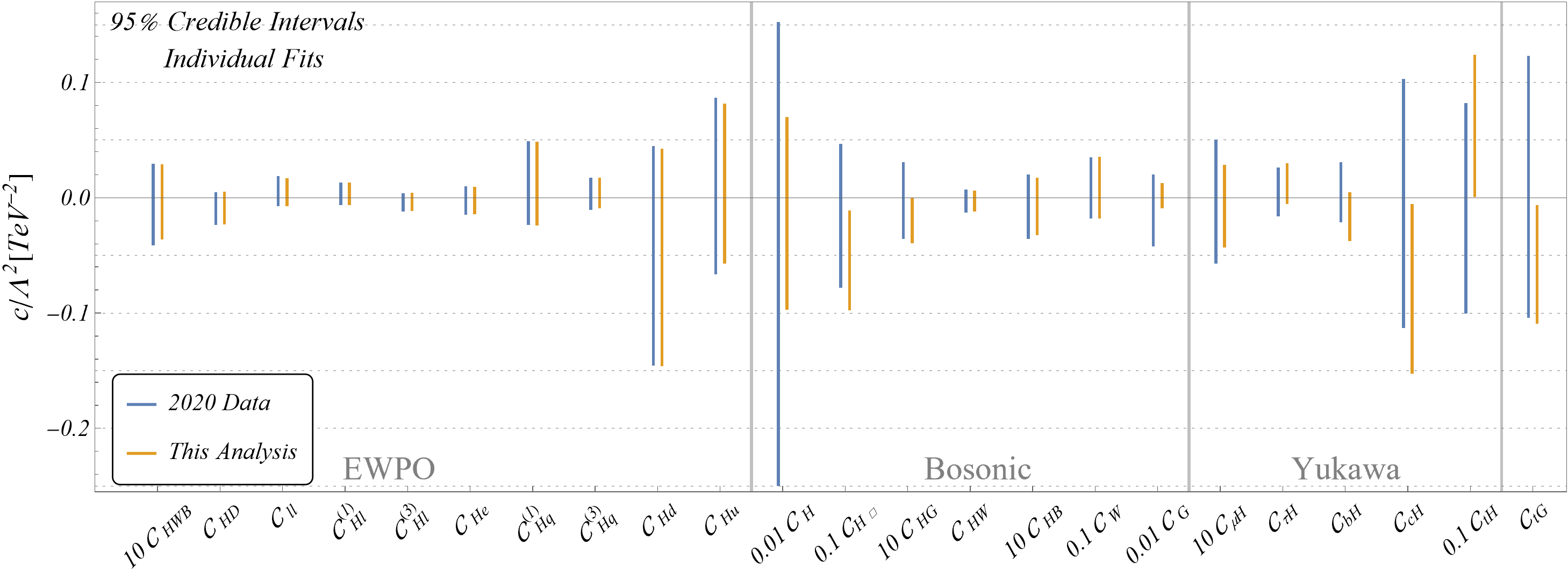
We start the discussion of our model-independent fits by showing the results of one-parameter fits of the WCs in the upper panel of fig. 3, see also tab. 24 for numerical results. In the figure, we contrast the results including our full dataset with a reduced set based on the one used in the most recent fitmaker analysis Ellis:2020unq . See tab. 1 for the exact dataset definitions. Overall, the WCs constrained through the EWPO typically receive much stronger individual bounds than those constrained through Higgs and di-boson observables alone. The most weakly constrained WC is 𝒞Hsubscript𝒞𝐻\mathcal{C}_{H} which is most strongly constrained through di-Higgs production in our fit. Comparing the two fits, we find that operators constrained through EWPO have not benefited from the addition of new datasets at the level of one-parameter fits. Several of the limits on the bosonic as well as Yukawa-like operators, on the other hand, have improved significantly. Deviations from the SM for some WCs, for instance for 𝒞tHsubscript𝒞𝑡𝐻\mathcal{C}_{tH}, are caused by large correlations in the CMS hZZ4𝑍𝑍4h\to ZZ\to 4\ell STXS analysis CMS:2021ugl , specifically between the ggF 1jet (pTH[0, 60]superscriptsubscript𝑝𝑇𝐻060p_{T}^{H}\in[0,\,60] GeV), ggF 1jet (pTH[60, 120]superscriptsubscript𝑝𝑇𝐻60120p_{T}^{H}\in[60,\,120] GeV), and qqH 2jet (mjj[0, 350]subscript𝑚𝑗𝑗0350m_{jj}\in[0,\,350] GeV, Vh𝑉Vh veto) regions. However, in the global analysis with more DOF none of these deviations persist.
Refer to caption
(a)
Refer to caption
(b)
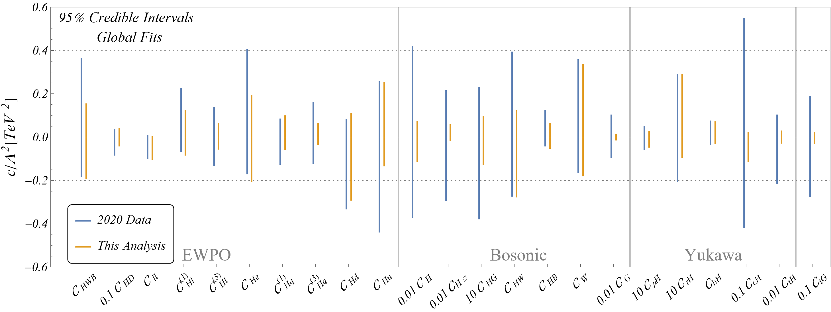
Figure 3: Individual (top) and global (bottom) 95% CI limits on the WCs. We compare a fit involving our full dataset (orange), with a reduced set containing LHC Higgs measurements up to year 2020 (blue), see tab. 1 for the dataset definitions. Note that some bounds have been scaled by factors of ten to fit all results on the same y𝑦y-axis.

In the lower panel of fig. 3, we display the results of our global fit of 232323 WCs after marginalisation. Numerical results can be found in tab. 24. To highlight the restriction power of recent STXS measurements, we again contrast our full data set with LHC data up to 2020. We have explicitly checked that the limits from this reduced dataset agree are in good agreement with previous literature Ellis:2020unq . The improvements of the limits with the addition of more data is even more visible in the global fit than it was in the one-parameter fits. We find relatively mild improvement for WCs describing modified Higgs Yukawa couplings to leptons or bottom quarks. Many of the other limits, however, have significantly decreased.

Comparing the limits from one-parameter fits with the global analysis, we find that the limits of six WCs weaken by a factor of ten or more compared to the individual fit limits: 𝒞HWBsubscript𝒞𝐻𝑊𝐵\mathcal{C}_{HWB}, 𝒞HDsubscript𝒞𝐻𝐷\mathcal{C}_{HD}, 𝒞HWsubscript𝒞𝐻𝑊\mathcal{C}_{HW}, 𝒞HBsubscript𝒞𝐻𝐵\mathcal{C}_{HB}, 𝒞Hesubscript𝒞𝐻𝑒\mathcal{C}_{He}, 𝒞Hl(1)superscriptsubscript𝒞𝐻𝑙1\mathcal{C}_{Hl}^{(1)}. This is the result of the strong correlation of these coefficients as displayed in tab. 25. Many pairs of these WCs have absolute correlation coefficients of 0.8greater-than-or-equivalent-toabsent0.8\gtrsim 0.8 as a result of their joint contribution to the shifts of SM parameters.
Refer to caption
(a)
Refer to caption
(b)
Refer to caption
(c)
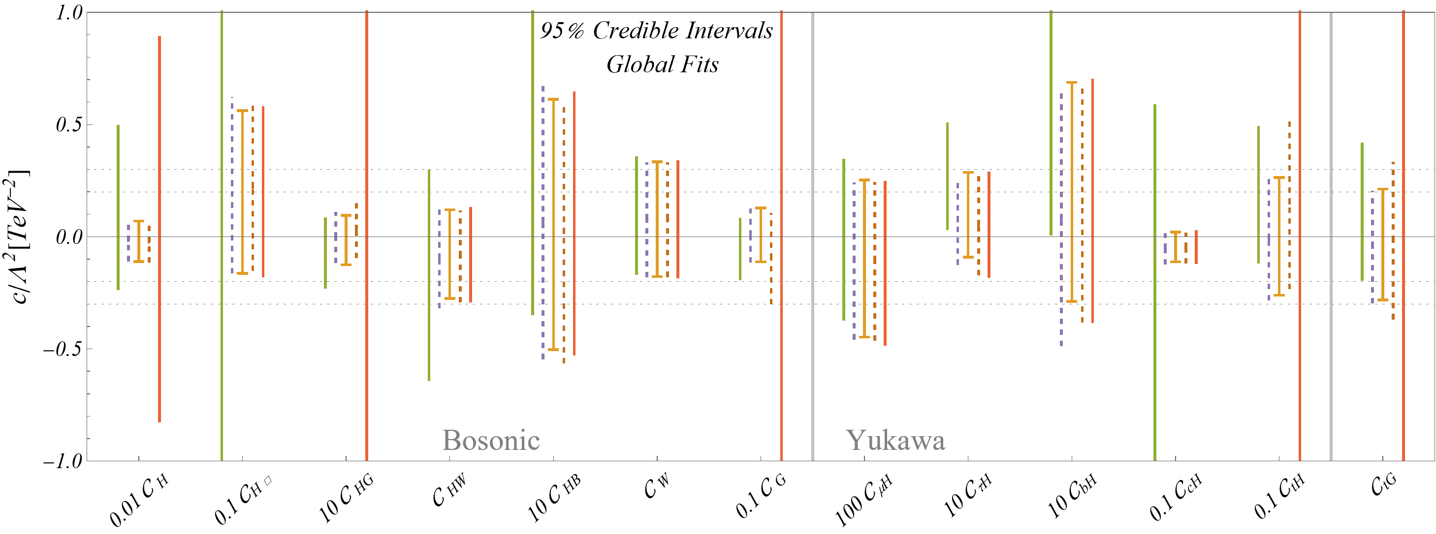
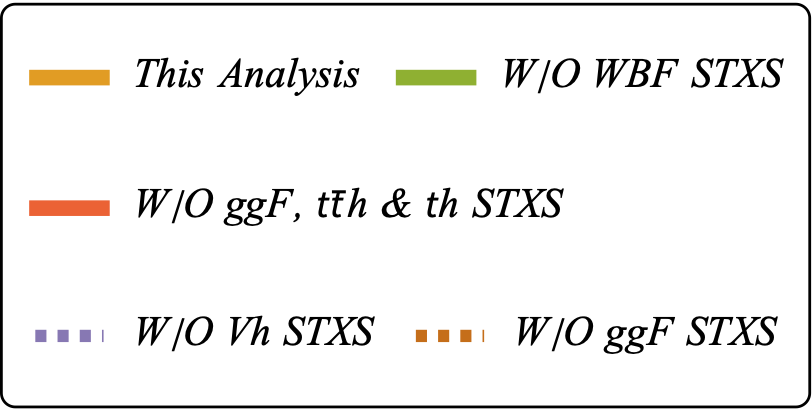
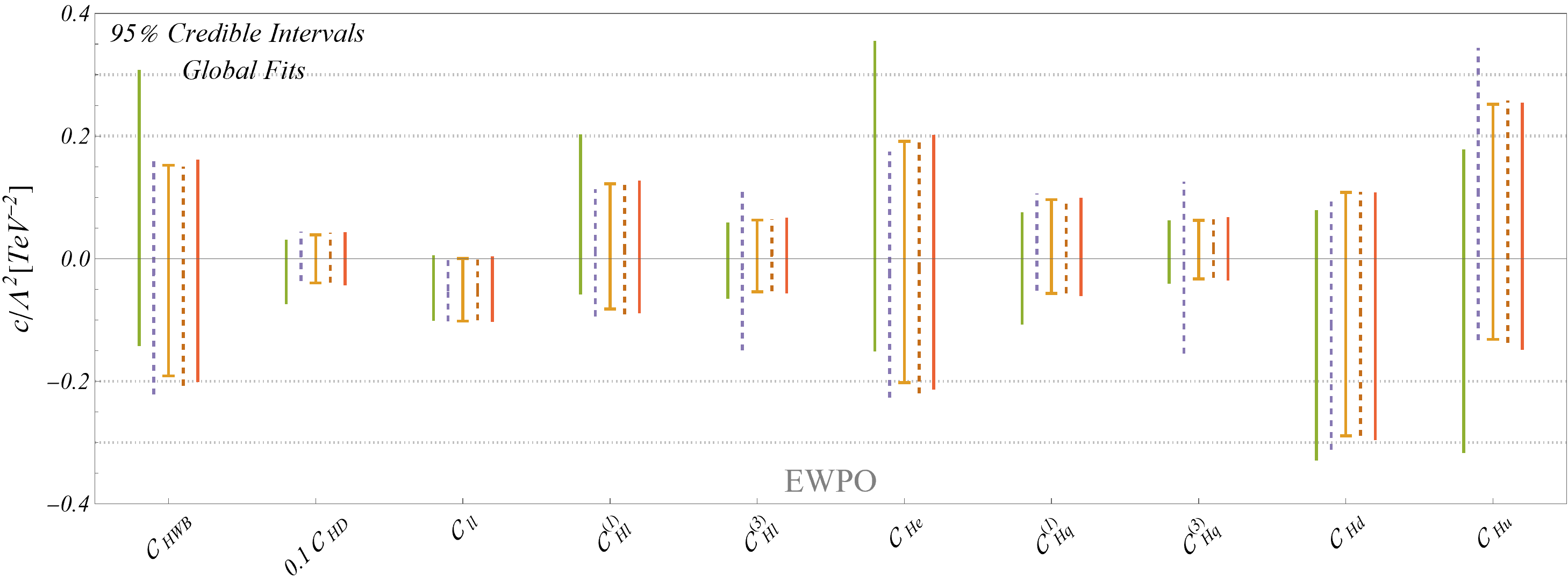
Figure 4: Figs. 4a and 4b show the 95%percent9595\% CIs on 23 WCs in a global fit using different datasets. We constrast the corresponding intervals obtained using the full dataset (orange) with datasets excluding certain sets of STXS measurements. We individually exclude STXS measurements of WBF production (green), Vh𝑉Vh measurements (purple), ggF measurements (red dashed), and a combination of ggF with tt¯h𝑡¯𝑡t\bar{t}h and th𝑡th (red solid). Note that some bounds have been scaled by factors of ten to fit all results on the same y𝑦y-axis.

To gain a better understanding for the relevance of different Higgs production channels for the constraints on different WCs, we display in fig. 4 the global fit limits on the WCs when removing certain STXS channels from the analysis. In four additional fits, we have removed the STXS channels for associated production of a Higgs with a vector boson (Vh𝑉Vh), weak boson fusion (WBF), gluon fusion (ggF), and a combination of gluon fusion as well as top associated production modes (ggF+tt¯h𝑡¯𝑡t\bar{t}h+tH𝑡𝐻tH). As expected, removing gluon fusion STXS channels from the analysis only weakens the limits on 𝒞tGsubscript𝒞𝑡𝐺\mathcal{C}_{tG}, 𝒞tHsubscript𝒞𝑡𝐻\mathcal{C}_{tH}, 𝒞Gsubscript𝒞𝐺\mathcal{C}_{G} and 𝒞HGsubscript𝒞𝐻𝐺\mathcal{C}_{HG}, highlighting the constraining power of ggF STXS measurements up to high transverse momenta of the Higgs. The highest-momentum STXS regions included in our analysis are pTH[200, 300, 450]GeVsuperscriptsubscript𝑝𝑇𝐻200300450GeVp_{T}^{H}\in[200,\,300,\,450]\,\text{GeV} as well as pTH>450GeVsuperscriptsubscript𝑝𝑇𝐻450GeVp_{T}^{H}>450\,\text{GeV} CMS:2021kom . When in addition to removing the gluon fusion STXS channels we also neglect top associated Higgs production, the extreme weakening of the limits on 𝒞HGsubscript𝒞𝐻𝐺\mathcal{C}_{HG} and 𝒞tHsubscript𝒞𝑡𝐻\mathcal{C}_{tH} leads to looser constraints on 𝒞Hsubscript𝒞𝐻\mathcal{C}_{H}. This is because of correlations of 𝒞Hsubscript𝒞𝐻\mathcal{C}_{H} with other WCs (𝒞tHsubscript𝒞𝑡𝐻\mathcal{C}_{tH} and 𝒞HGsubscript𝒞𝐻𝐺\mathcal{C}_{HG}) which are, however, irrelevant at the current level of constraints from ggF and top associated Higgs production.

STXS measurements of Vh𝑉Vh production mainly affect the limits of 𝒞Hq(3)superscriptsubscript𝒞𝐻𝑞3\mathcal{C}_{Hq}^{(3)}, 𝒞Husubscript𝒞𝐻𝑢\mathcal{C}_{Hu} and 𝒞Hl(3)superscriptsubscript𝒞𝐻𝑙3\mathcal{C}_{Hl}^{(3)}. While 𝒞Hq(3)superscriptsubscript𝒞𝐻𝑞3\mathcal{C}_{Hq}^{(3)} and 𝒞Husubscript𝒞𝐻𝑢\mathcal{C}_{Hu} directly profit from Vh𝑉Vh measurements at high pTVsuperscriptsubscript𝑝𝑇𝑉p_{T}^{V}, 𝒞Hl(3)superscriptsubscript𝒞𝐻𝑙3\mathcal{C}_{Hl}^{(3)} improves indirectly as it is highly correlated with 𝒞Hq(3)superscriptsubscript𝒞𝐻𝑞3\mathcal{C}_{Hq}^{(3)}. WBF STXS measurements influence several bosonic operators such as 𝒞Hsubscript𝒞𝐻\mathcal{C}_{H\square} and 𝒞HWBsubscript𝒞𝐻𝑊𝐵\mathcal{C}_{HWB}. Other operators which do not directly contribute to WBF, for instance 𝒞Hl(1)superscriptsubscript𝒞𝐻𝑙1\mathcal{C}_{Hl}^{(1)} are affected by WBF STXS measurements through their correlation with other operators. 𝒞cHsubscript𝒞𝑐𝐻\mathcal{C}_{cH}, which only appears in the parametrisation of the Higgs width, is highly affected by WBF STXS data because of its correlation with 𝒞Hsubscript𝒞𝐻\mathcal{C}_{H\square}.

5 BSMs CoDExCoDExabsent\xrightarrow{\texttt{CoDEx}}\;\subset SMEFT: Effective Operators, WCs and Bayesian Analysis

Table 2: SM and BSM fields and their spin and gauge quantum numbers. The BSM Lagrangians are constructed using these fields.
SM field Spin SM quantum numbers
SU(3)C𝑆𝑈subscript3𝐶SU(3)_{{}_{C}} SU(2)L𝑆𝑈subscript2𝐿SU(2)_{{}_{L}} U(1)Y𝑈subscript1𝑌U(1)_{{}_{Y}}1
qLsubscript𝑞𝐿q_{{}_{L}} 1212\frac{1}{2} 3 2 1616\frac{1}{6}
lLsubscript𝑙𝐿l_{{}_{L}} 1212\frac{1}{2} 1 2 -1212\frac{1}{2}
uRsubscript𝑢𝑅u_{{}_{R}} 1212\frac{1}{2} 3 1 2323\frac{2}{3}
dRsubscript𝑑𝑅d_{{}_{R}} 1212\frac{1}{2} 3 1 -1313\frac{1}{3}
eRsubscript𝑒𝑅e_{{}_{R}} 1212\frac{1}{2} 1 1 -1
H𝐻H 0 1 2 1212\frac{1}{2}
Bμνsubscript𝐵𝜇𝜈B_{\mu\nu} 1 1 1 0
Wμνsubscript𝑊𝜇𝜈W_{\mu\nu} 1 1 3 0
Gμνsubscript𝐺𝜇𝜈G_{\mu\nu} 1 8 1 0
  • 1

    Hypercharge convention: Qemsubscript𝑄emQ_{\text{em}} = T3subscript𝑇3T_{3} + Y, where Qemsubscript𝑄emQ_{\text{em}}, T3subscript𝑇3T_{3} and Y are electro-magnetic charge, third component of isospin quantum number and hypercharge respectively.

(a)
BSM field Spin SM quantum numbers Mass
SU(3)C𝑆𝑈subscript3𝐶SU(3)_{{}_{C}} SU(2)L𝑆𝑈subscript2𝐿SU(2)_{{}_{L}} U(1)Y𝑈subscript1𝑌U(1)_{{}_{Y}}
𝒮𝒮\mathcal{S} 0 1 1 0 m𝒮subscript𝑚𝒮m_{\mathcal{S}}
ΔΔ\Delta 0 1 3 0 mΔsubscript𝑚Δm_{\Delta}
𝒮1subscript𝒮1\mathcal{S}_{1} 0 1 1 1 m𝒮1subscript𝑚subscript𝒮1m_{\mathcal{S}_{1}}
𝒮2subscript𝒮2\mathcal{S}_{2} 0 1 1 2 m𝒮2subscript𝑚subscript𝒮2m_{\mathcal{S}_{2}}
Δ1subscriptΔ1\Delta_{1} 0 1 3 1 mΔ1subscript𝑚subscriptΔ1m_{\Delta_{1}}
2subscript2\mathcal{H}_{2} 0 1 2 1212-\frac{1}{2} m2subscript𝑚subscript2m_{\mathcal{H}_{2}}
ΣΣ\Sigma 0 1 4 1212\frac{1}{2} mΣsubscript𝑚Σm_{{}_{\Sigma}}
φ1subscript𝜑1\varphi_{1} 0 3 1 1313-\frac{1}{3} mφ1subscript𝑚subscript𝜑1m_{\varphi_{1}}
φ2subscript𝜑2\varphi_{2} 0 3 1 4343-\frac{4}{3} mφ2subscript𝑚subscript𝜑2m_{\varphi_{2}}
Θ1subscriptΘ1\Theta_{1} 0 3 2 1616\frac{1}{6} mΘ1subscript𝑚subscriptΘ1m_{\Theta_{1}}
Θ2subscriptΘ2\Theta_{2} 0 3 2 7676\frac{7}{6} mΘ2subscript𝑚subscriptΘ2m_{\Theta_{2}}
ΩΩ\Omega 0 3 3 1313-\frac{1}{3} mΩsubscript𝑚Ωm_{\Omega}
χ1subscript𝜒1\chi_{{}_{1}} 0 6 3 1313\frac{1}{3} mχ1subscript𝑚subscript𝜒1m_{\chi_{{}_{1}}}
χ2subscript𝜒2\chi_{{}_{2}} 0 6 1 4343\frac{4}{3} mχ2subscript𝑚subscript𝜒2m_{\chi_{{}_{2}}}
χ3subscript𝜒3\chi_{{}_{3}} 0 6 1 2323-\frac{2}{3} mχ3subscript𝑚subscript𝜒3m_{\chi_{{}_{3}}}
χ4subscript𝜒4\chi_{{}_{4}} 0 6 1 1313\frac{1}{3} mχ4subscript𝑚subscript𝜒4m_{\chi_{{}_{4}}}
(b)
Refer to caption
(a) λ2,1subscript𝜆subscript21\lambda_{\mathcal{H}_{2},1} - λ2,2subscript𝜆subscript22\lambda_{\mathcal{H}_{2},2}
Refer to caption
(b) λ2,2subscript𝜆subscript22\lambda_{\mathcal{H}_{2},2} - λ2,3subscript𝜆subscript23\lambda_{\mathcal{H}_{2},3}
Refer to caption
(c) λ2,1subscript𝜆subscript21\lambda_{\mathcal{H}_{2},1} - λ2,3subscript𝜆subscript23\lambda_{\mathcal{H}_{2},3}
Refer to caption
(d) ηΘ1(1)superscriptsubscript𝜂subscriptΘ11\eta_{\Theta_{1}}^{(1)} - ηΘ1(2)superscriptsubscript𝜂subscriptΘ12\eta_{\Theta_{1}}^{(2)}
Refer to caption
(e) Legend
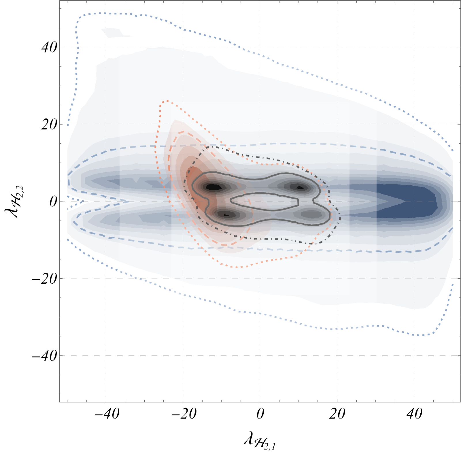
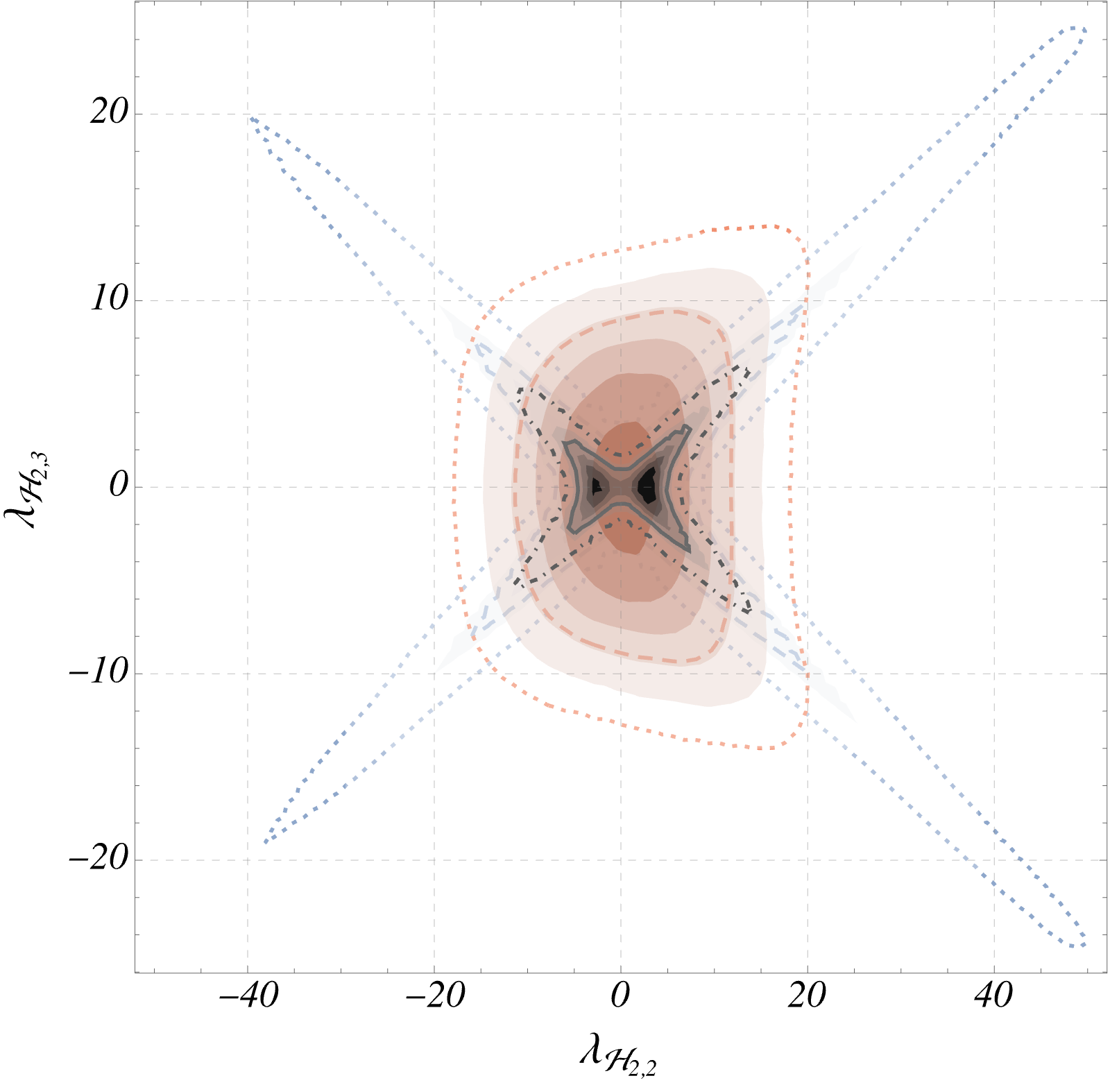
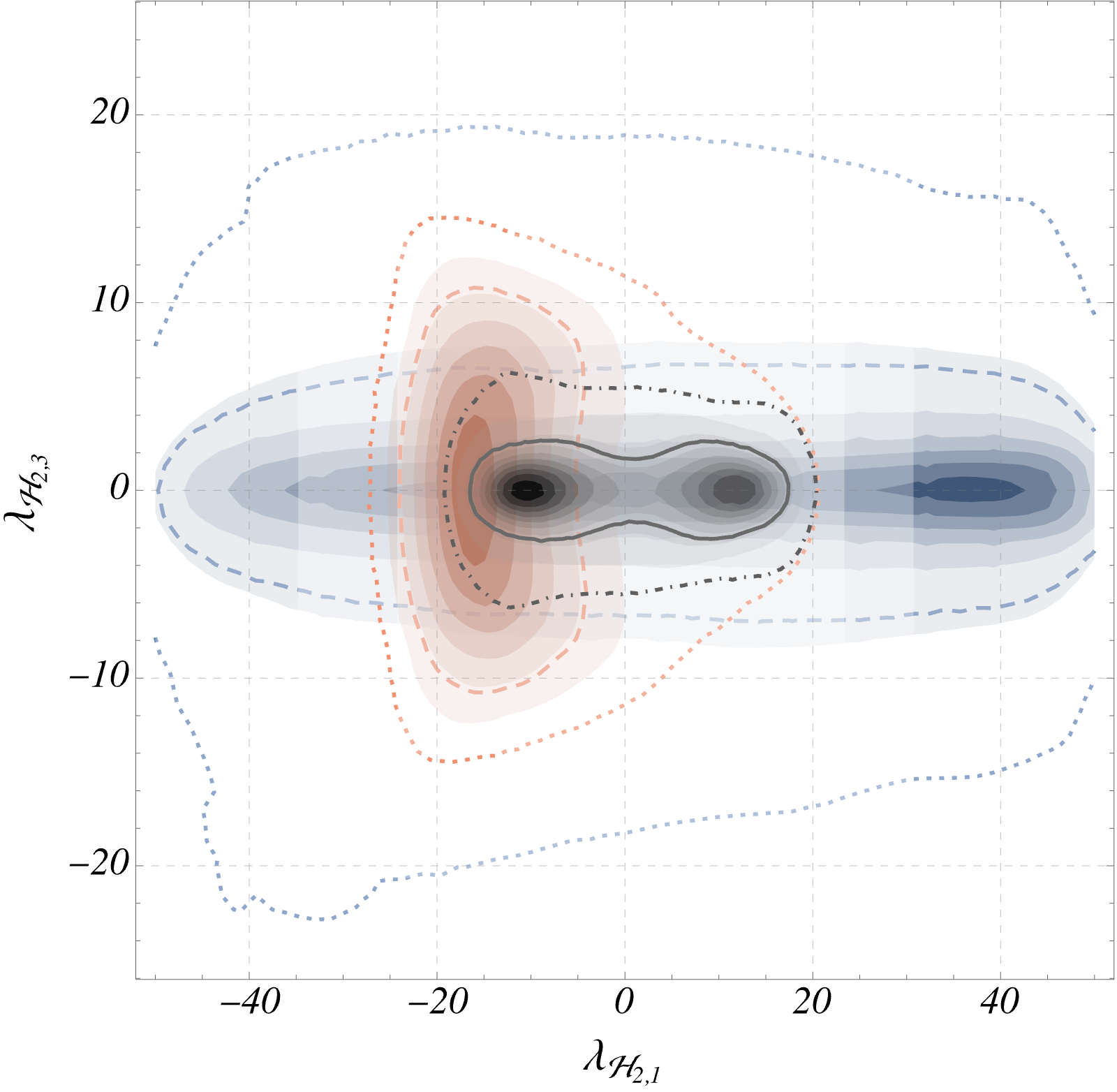
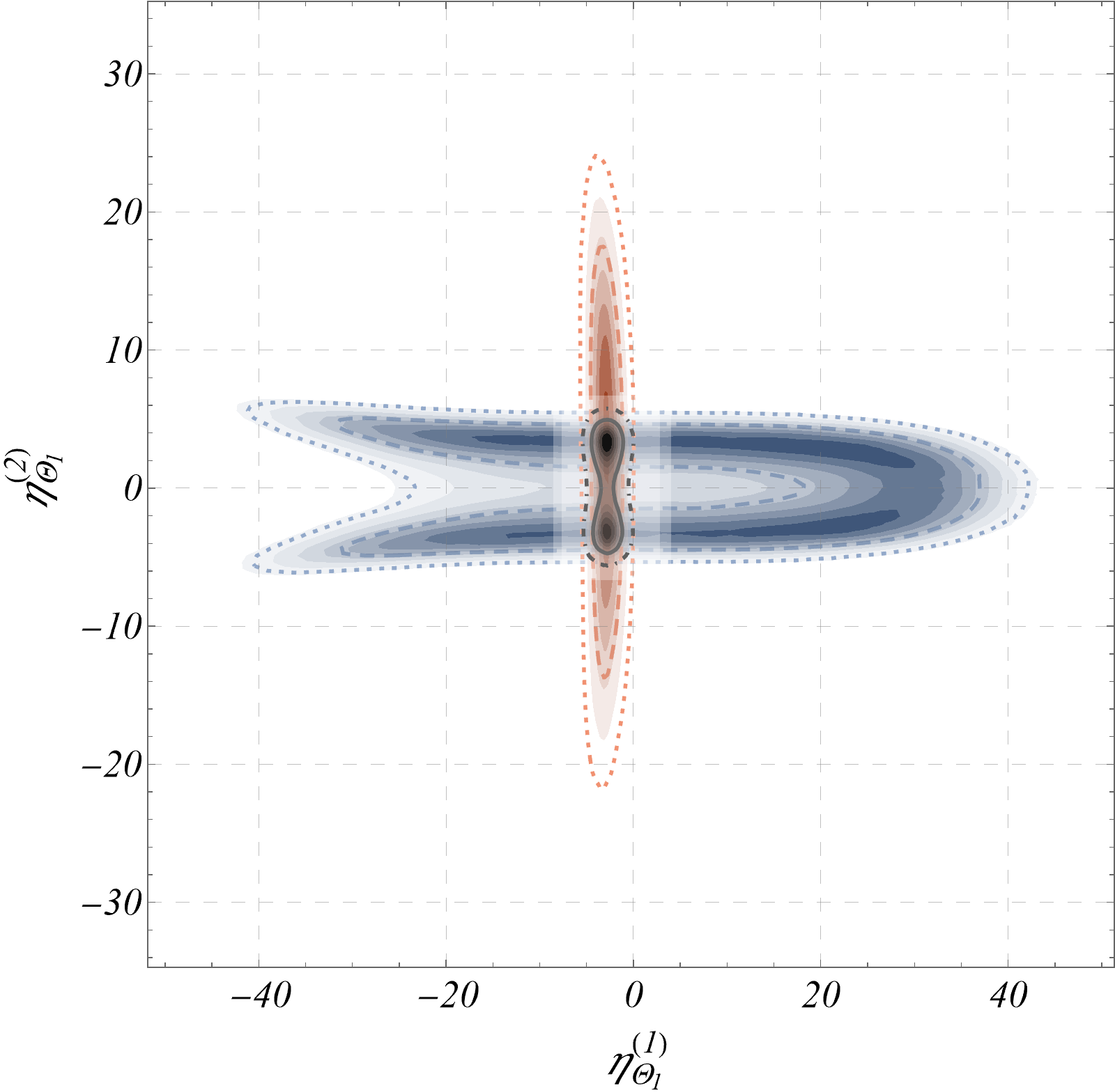
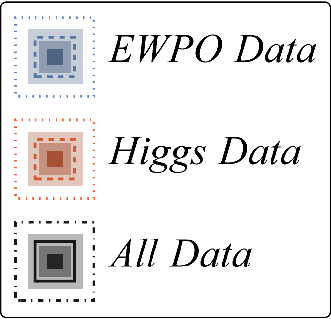
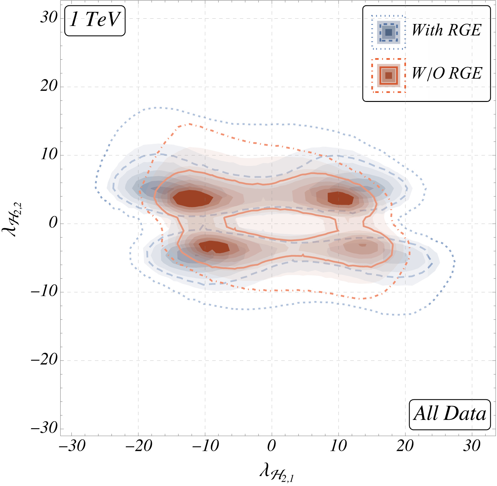
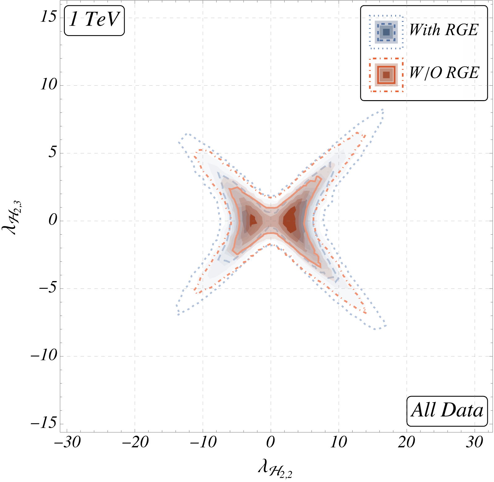
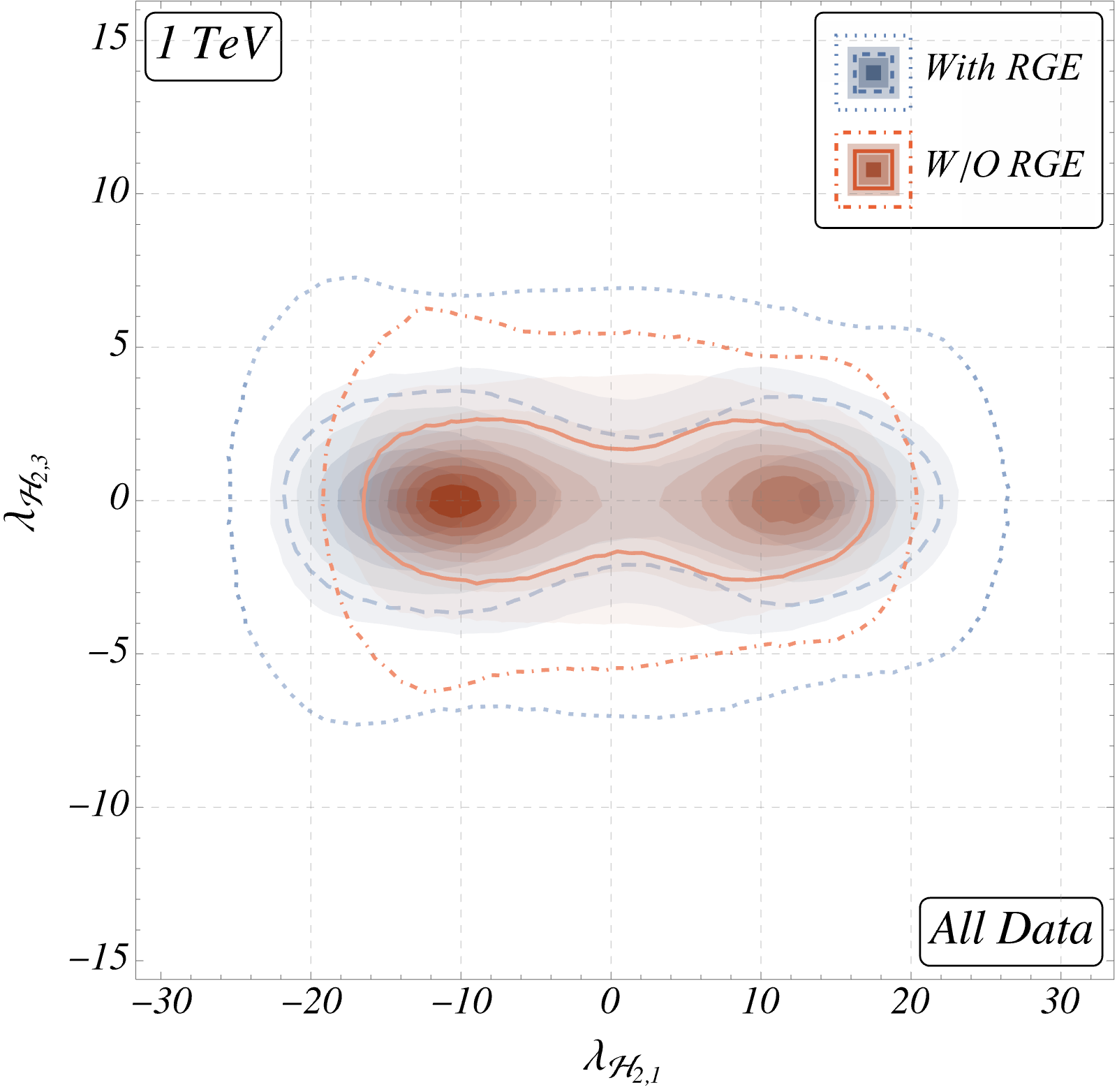
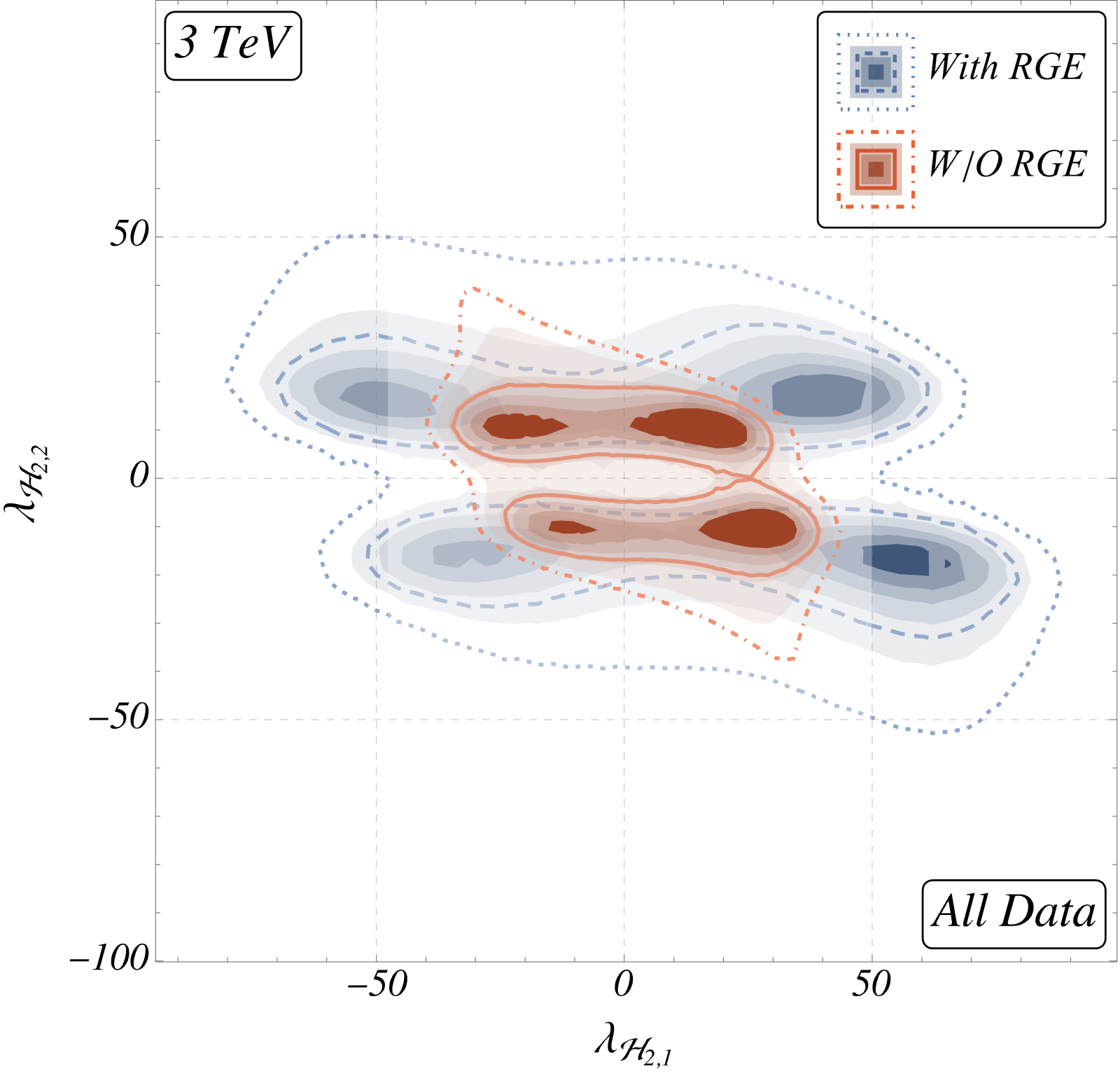
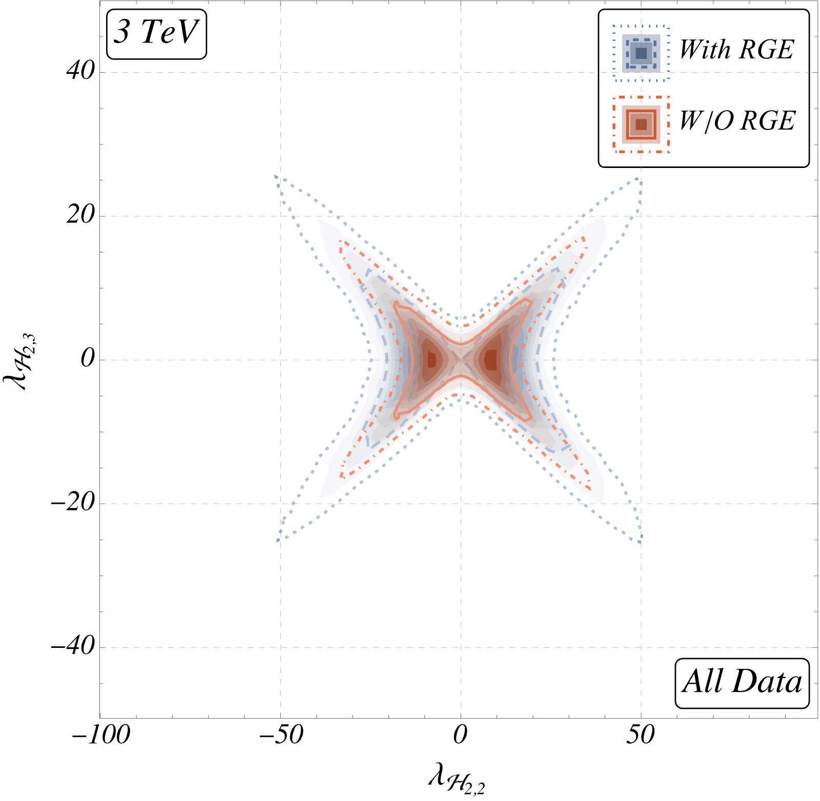
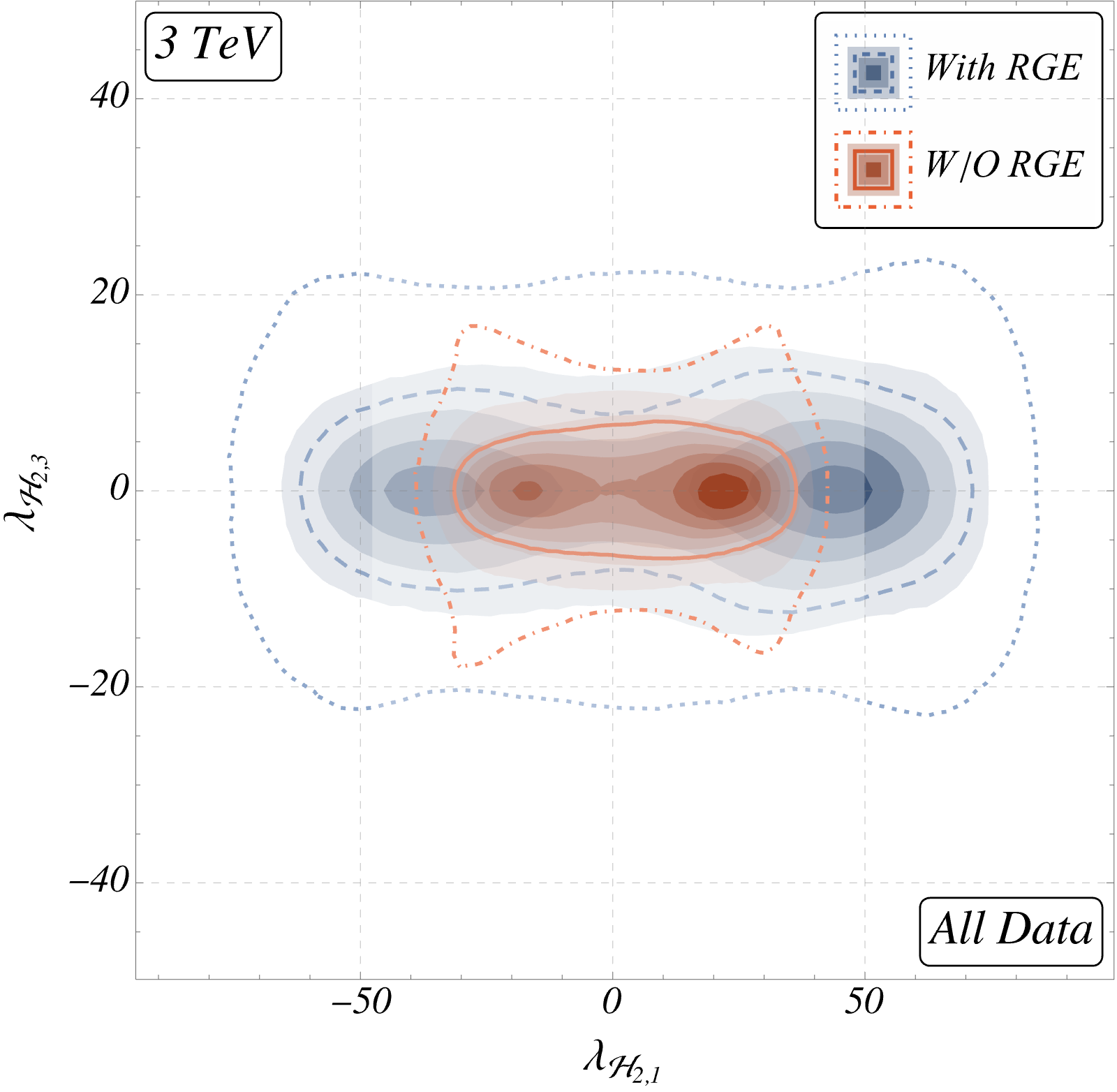
Figure 5: Two-dimensional marginalised posteriors among the BSM parameters for 2subscript2\mathcal{H}_{2} (top row) and Θ1subscriptΘ1\Theta_{1}. The line contours represent the 68% and 95% credible intervals (CIs) and the filled contours with changing opacity show the high-probability regions with decreasing probabilities (darker to lighter). We show the results from a fit of “EWPO” data only (blue), “Higgs” data only (red) as well as for “All” (black).
Table 3: Warsaw basis effective operators and the associated WCs that emerge after integrating-out the heavy field 2:(1,2,12):subscript21212\mathcal{H}_{2}:(1,2,-\frac{1}{2}). Operators highlighted in red do not affect our current set of observables and are thus absent from our analysis. Operators highlighted in blue are functions of SM parameters only, while the red coloured ones do not contribute to our observables.
Dim-6 Ops. Wilson coefficients
QdHsubscript𝑄dHQ_{\text{dH}} ηH2YdSM16π2m223ηHη2YdSM16π2m22ηHY2(d)m22superscriptsubscript𝜂𝐻2superscriptsubscript𝑌𝑑SM16superscript𝜋2superscriptsubscript𝑚subscript223subscript𝜂𝐻subscript𝜂subscript2superscriptsubscript𝑌𝑑SM16superscript𝜋2superscriptsubscript𝑚subscript22subscript𝜂𝐻superscriptsubscript𝑌subscript2𝑑superscriptsubscript𝑚subscript22\frac{\eta_{H}^{2}Y_{d}^{\text{SM}}}{16\pi^{2}m_{\mathcal{H}_{2}}^{2}}-\frac{3\eta_{H}\eta_{\mathcal{H}_{2}}Y_{d}^{\text{SM}}}{16\pi^{2}m_{\mathcal{H}_{2}}^{2}}-\frac{\eta_{H}Y_{\mathcal{H}_{2}}^{(d)}}{m_{\mathcal{H}_{2}}^{2}}
3ηHλ2Y2(d)32π2m22+3ηHλ2,1Y2(d)16π2m223η2λ2,1Y2(d)16π2m223subscript𝜂𝐻subscript𝜆subscript2superscriptsubscript𝑌subscript2𝑑32superscript𝜋2superscriptsubscript𝑚subscript223subscript𝜂𝐻subscript𝜆subscript21superscriptsubscript𝑌subscript2𝑑16superscript𝜋2superscriptsubscript𝑚subscript223subscript𝜂subscript2subscript𝜆subscript21superscriptsubscript𝑌subscript2𝑑16superscript𝜋2superscriptsubscript𝑚subscript22-\frac{3\eta_{H}\lambda_{\mathcal{H}_{2}}Y_{\mathcal{H}_{2}}^{(d)}}{32\pi^{2}m_{\mathcal{H}_{2}}^{2}}+\frac{3\eta_{H}\lambda_{\mathcal{H}_{2},1}Y_{\mathcal{H}_{2}}^{(d)}}{16\pi^{2}m_{\mathcal{H}_{2}}^{2}}-\frac{3\eta_{\mathcal{H}_{2}}\lambda_{\mathcal{H}_{2},1}Y_{\mathcal{H}_{2}}^{(d)}}{16\pi^{2}m_{\mathcal{H}_{2}}^{2}}
ηHλ2,2Y2(d)4π2m223η2λ2,2Y2(d)16π2m22+λ2,22YdSM192π2m22subscript𝜂𝐻subscript𝜆subscript22superscriptsubscript𝑌subscript2𝑑4superscript𝜋2superscriptsubscript𝑚subscript223subscript𝜂subscript2subscript𝜆subscript22superscriptsubscript𝑌subscript2𝑑16superscript𝜋2superscriptsubscript𝑚subscript22superscriptsubscript𝜆subscript222superscriptsubscript𝑌𝑑SM192superscript𝜋2superscriptsubscript𝑚subscript22\frac{\eta_{H}\lambda_{\mathcal{H}_{2},2}Y_{\mathcal{H}_{2}}^{(d)}}{4\pi^{2}m_{\mathcal{H}_{2}}^{2}}-\frac{3\eta_{\mathcal{H}_{2}}\lambda_{\mathcal{H}_{2},2}Y_{\mathcal{H}_{2}}^{(d)}}{16\pi^{2}m_{\mathcal{H}_{2}}^{2}}+\frac{\lambda_{\mathcal{H}_{2},2}^{2}Y_{d}^{\text{SM}}}{192\pi^{2}m_{\mathcal{H}_{2}}^{2}}
5ηHλ2,3Y2(d)8π2m22+λ2,32YdSM48π2m225subscript𝜂𝐻subscript𝜆subscript23superscriptsubscript𝑌subscript2𝑑8superscript𝜋2superscriptsubscript𝑚subscript22superscriptsubscript𝜆subscript232superscriptsubscript𝑌𝑑SM48superscript𝜋2superscriptsubscript𝑚subscript22\frac{5\eta_{H}\lambda_{\mathcal{H}_{2},3}Y_{\mathcal{H}_{2}}^{(d)}}{8\pi^{2}m_{\mathcal{H}_{2}}^{2}}+\frac{\lambda_{\mathcal{H}_{2},3}^{2}Y_{d}^{\text{SM}}}{48\pi^{2}m_{\mathcal{H}_{2}}^{2}}
QeHsubscript𝑄eHQ_{\text{eH}} ηH2YeSM16π2m223ηHη2YeSM16π2m22ηHY2(e)m22superscriptsubscript𝜂𝐻2superscriptsubscript𝑌𝑒SM16superscript𝜋2superscriptsubscript𝑚subscript223subscript𝜂𝐻subscript𝜂subscript2superscriptsubscript𝑌𝑒SM16superscript𝜋2superscriptsubscript𝑚subscript22subscript𝜂𝐻superscriptsubscript𝑌subscript2𝑒superscriptsubscript𝑚subscript22\frac{\eta_{H}^{2}Y_{e}^{\text{SM}}}{16\pi^{2}m_{\mathcal{H}_{2}}^{2}}-\frac{3\eta_{H}\eta_{\mathcal{H}_{2}}Y_{e}^{\text{SM}}}{16\pi^{2}m_{\mathcal{H}_{2}}^{2}}-\frac{\eta_{H}Y_{\mathcal{H}_{2}}^{(e)}}{m_{\mathcal{H}_{2}}^{2}}
3ηHλ2Y2(e)32π2m22+3ηHλ2,1Y2(e)16π2m223η2λ2,1Y2(e)16π2m223subscript𝜂𝐻subscript𝜆subscript2superscriptsubscript𝑌subscript2𝑒32superscript𝜋2superscriptsubscript𝑚subscript223subscript𝜂𝐻subscript𝜆subscript21superscriptsubscript𝑌subscript2𝑒16superscript𝜋2superscriptsubscript𝑚subscript223subscript𝜂subscript2subscript𝜆subscript21superscriptsubscript𝑌subscript2𝑒16superscript𝜋2superscriptsubscript𝑚subscript22-\frac{3\eta_{H}\lambda_{\mathcal{H}_{2}}Y_{\mathcal{H}_{2}}^{(e)}}{32\pi^{2}m_{\mathcal{H}_{2}}^{2}}+\frac{3\eta_{H}\lambda_{\mathcal{H}_{2},1}Y_{\mathcal{H}_{2}}^{(e)}}{16\pi^{2}m_{\mathcal{H}_{2}}^{2}}-\frac{3\eta_{\mathcal{H}_{2}}\lambda_{\mathcal{H}_{2},1}Y_{\mathcal{H}_{2}}^{(e)}}{16\pi^{2}m_{\mathcal{H}_{2}}^{2}}
ηHλ2,2Y2(e)4π2m223η2λ2,2Y2(e)16π2m22+λ2,22YeSM192π2m22subscript𝜂𝐻subscript𝜆subscript22superscriptsubscript𝑌subscript2𝑒4superscript𝜋2superscriptsubscript𝑚subscript223subscript𝜂subscript2subscript𝜆subscript22superscriptsubscript𝑌subscript2𝑒16superscript𝜋2superscriptsubscript𝑚subscript22superscriptsubscript𝜆subscript222superscriptsubscript𝑌𝑒SM192superscript𝜋2superscriptsubscript𝑚subscript22\frac{\eta_{H}\lambda_{\mathcal{H}_{2},2}Y_{\mathcal{H}_{2}}^{(e)}}{4\pi^{2}m_{\mathcal{H}_{2}}^{2}}-\frac{3\eta_{\mathcal{H}_{2}}\lambda_{\mathcal{H}_{2},2}Y_{\mathcal{H}_{2}}^{(e)}}{16\pi^{2}m_{\mathcal{H}_{2}}^{2}}+\frac{\lambda_{\mathcal{H}_{2},2}^{2}Y_{e}^{\text{SM}}}{192\pi^{2}m_{\mathcal{H}_{2}}^{2}}
5ηHλ2,3Y2(e)8π2m22+λ2,32YeSM48π2m225subscript𝜂𝐻subscript𝜆subscript23superscriptsubscript𝑌subscript2𝑒8superscript𝜋2superscriptsubscript𝑚subscript22superscriptsubscript𝜆subscript232superscriptsubscript𝑌𝑒SM48superscript𝜋2superscriptsubscript𝑚subscript22\frac{5\eta_{H}\lambda_{\mathcal{H}_{2},3}Y_{\mathcal{H}_{2}}^{(e)}}{8\pi^{2}m_{\mathcal{H}_{2}}^{2}}+\frac{\lambda_{\mathcal{H}_{2},3}^{2}Y_{e}^{\text{SM}}}{48\pi^{2}m_{\mathcal{H}_{2}}^{2}}
QuHsubscript𝑄uHQ_{\text{uH}} ηH2YuSM16π2m22+3ηHλ2Y2(u)32π2m22+ηHY2(u)m22superscriptsubscript𝜂𝐻2superscriptsubscript𝑌𝑢SM16superscript𝜋2superscriptsubscript𝑚subscript223subscript𝜂𝐻subscript𝜆subscript2superscriptsubscript𝑌subscript2𝑢32superscript𝜋2superscriptsubscript𝑚subscript22subscript𝜂𝐻superscriptsubscript𝑌subscript2𝑢superscriptsubscript𝑚subscript22\frac{\eta_{H}^{2}Y_{u}^{\text{SM}}}{16\pi^{2}m_{\mathcal{H}_{2}}^{2}}+\frac{3\eta_{H}\lambda_{\mathcal{H}_{2}}Y_{\mathcal{H}_{2}}^{(u)}}{32\pi^{2}m_{\mathcal{H}_{2}}^{2}}+\frac{\eta_{H}Y_{\mathcal{H}_{2}}^{(u)}}{m_{\mathcal{H}_{2}}^{2}}
3ηHη2YuSM16π2m223ηHλ2,1Y2(u)16π2m22+3η2λ2,1Y2(u)16π2m223subscript𝜂𝐻subscript𝜂subscript2superscriptsubscript𝑌𝑢SM16superscript𝜋2superscriptsubscript𝑚subscript223subscript𝜂𝐻subscript𝜆subscript21superscriptsubscript𝑌subscript2𝑢16superscript𝜋2superscriptsubscript𝑚subscript223subscript𝜂subscript2subscript𝜆subscript21superscriptsubscript𝑌subscript2𝑢16superscript𝜋2superscriptsubscript𝑚subscript22-\frac{3\eta_{H}\eta_{\mathcal{H}_{2}}Y_{u}^{\text{SM}}}{16\pi^{2}m_{\mathcal{H}_{2}}^{2}}-\frac{3\eta_{H}\lambda_{\mathcal{H}_{2},1}Y_{\mathcal{H}_{2}}^{(u)}}{16\pi^{2}m_{\mathcal{H}_{2}}^{2}}+\frac{3\eta_{\mathcal{H}_{2}}\lambda_{\mathcal{H}_{2},1}Y_{\mathcal{H}_{2}}^{(u)}}{16\pi^{2}m_{\mathcal{H}_{2}}^{2}}
ηHλ2,2Y2(u)4π2m22+3η2λ2,2Y2(u)16π2m22+λ2,22YuSM192π2m22subscript𝜂𝐻subscript𝜆subscript22superscriptsubscript𝑌subscript2𝑢4superscript𝜋2superscriptsubscript𝑚subscript223subscript𝜂subscript2subscript𝜆subscript22superscriptsubscript𝑌subscript2𝑢16superscript𝜋2superscriptsubscript𝑚subscript22superscriptsubscript𝜆subscript222superscriptsubscript𝑌𝑢SM192superscript𝜋2superscriptsubscript𝑚subscript22-\frac{\eta_{H}\lambda_{\mathcal{H}_{2},2}Y_{\mathcal{H}_{2}}^{(u)}}{4\pi^{2}m_{\mathcal{H}_{2}}^{2}}+\frac{3\eta_{\mathcal{H}_{2}}\lambda_{\mathcal{H}_{2},2}Y_{\mathcal{H}_{2}}^{(u)}}{16\pi^{2}m_{\mathcal{H}_{2}}^{2}}+\frac{\lambda_{\mathcal{H}_{2},2}^{2}Y_{u}^{\text{SM}}}{192\pi^{2}m_{\mathcal{H}_{2}}^{2}}
λ2,32YuSM48π2m225ηHλ2,3Y2(u)8π2m22superscriptsubscript𝜆subscript232superscriptsubscript𝑌𝑢SM48superscript𝜋2superscriptsubscript𝑚subscript225subscript𝜂𝐻subscript𝜆subscript23superscriptsubscript𝑌subscript2𝑢8superscript𝜋2superscriptsubscript𝑚subscript22\frac{\lambda_{\mathcal{H}_{2},3}^{2}Y_{u}^{\text{SM}}}{48\pi^{2}m_{\mathcal{H}_{2}}^{2}}-\frac{5\eta_{H}\lambda_{\mathcal{H}_{2},3}Y_{\mathcal{H}_{2}}^{(u)}}{8\pi^{2}m_{\mathcal{H}_{2}}^{2}}
QHsubscript𝑄𝐻Q_{H} 3ηH2λ232π2m22+17ηH2λHSM16π2m22+ηH2m223superscriptsubscript𝜂𝐻2subscript𝜆subscript232superscript𝜋2superscriptsubscript𝑚subscript2217superscriptsubscript𝜂𝐻2superscriptsubscript𝜆𝐻SM16superscript𝜋2superscriptsubscript𝑚subscript22superscriptsubscript𝜂𝐻2superscriptsubscript𝑚subscript22\frac{3\eta_{H}^{2}\lambda_{\mathcal{H}_{2}}}{32\pi^{2}m_{\mathcal{H}_{2}}^{2}}+\frac{17\eta_{H}^{2}\lambda_{H}^{\text{SM}}}{16\pi^{2}m_{\mathcal{H}_{2}}^{2}}+\frac{\eta_{H}^{2}}{m_{\mathcal{H}_{2}}^{2}}
3ηH2λ2,14π2m223ηHη2λHSM8π2m22+3ηHη2λ2,18π2m223superscriptsubscript𝜂𝐻2subscript𝜆subscript214superscript𝜋2superscriptsubscript𝑚subscript223subscript𝜂𝐻subscript𝜂subscript2superscriptsubscript𝜆𝐻SM8superscript𝜋2superscriptsubscript𝑚subscript223subscript𝜂𝐻subscript𝜂subscript2subscript𝜆subscript218superscript𝜋2superscriptsubscript𝑚subscript22-\frac{3\eta_{H}^{2}\lambda_{\mathcal{H}_{2},1}}{4\pi^{2}m_{\mathcal{H}_{2}}^{2}}-\frac{3\eta_{H}\eta_{\mathcal{H}_{2}}\lambda_{H}^{\text{SM}}}{8\pi^{2}m_{\mathcal{H}_{2}}^{2}}+\frac{3\eta_{H}\eta_{\mathcal{H}_{2}}\lambda_{\mathcal{H}_{2},1}}{8\pi^{2}m_{\mathcal{H}_{2}}^{2}}
13ηH2λ2,216π2m22+3ηHη2λ2,28π2m22λ2,1348π2m2213superscriptsubscript𝜂𝐻2subscript𝜆subscript2216superscript𝜋2superscriptsubscript𝑚subscript223subscript𝜂𝐻subscript𝜂subscript2subscript𝜆subscript228superscript𝜋2superscriptsubscript𝑚subscript22superscriptsubscript𝜆subscript21348superscript𝜋2superscriptsubscript𝑚subscript22-\frac{13\eta_{H}^{2}\lambda_{\mathcal{H}_{2},2}}{16\pi^{2}m_{\mathcal{H}_{2}}^{2}}+\frac{3\eta_{H}\eta_{\mathcal{H}_{2}}\lambda_{\mathcal{H}_{2},2}}{8\pi^{2}m_{\mathcal{H}_{2}}^{2}}-\frac{\lambda_{\mathcal{H}_{2},1}^{3}}{48\pi^{2}m_{\mathcal{H}_{2}}^{2}}
λHSMλ2,2296π2m22λ2,12λ2,232π2m22λ2,1λ2,2232π2m22superscriptsubscript𝜆𝐻SMsuperscriptsubscript𝜆subscript22296superscript𝜋2superscriptsubscript𝑚subscript22superscriptsubscript𝜆subscript212subscript𝜆subscript2232superscript𝜋2superscriptsubscript𝑚subscript22subscript𝜆subscript21superscriptsubscript𝜆subscript22232superscript𝜋2superscriptsubscript𝑚subscript22\frac{\lambda_{H}^{\text{SM}}\lambda_{\mathcal{H}_{2},2}^{2}}{96\pi^{2}m_{\mathcal{H}_{2}}^{2}}-\frac{\lambda_{\mathcal{H}_{2},1}^{2}\lambda_{\mathcal{H}_{2},2}}{32\pi^{2}m_{\mathcal{H}_{2}}^{2}}-\frac{\lambda_{\mathcal{H}_{2},1}\lambda_{\mathcal{H}_{2},2}^{2}}{32\pi^{2}m_{\mathcal{H}_{2}}^{2}}
7ηH2λ2,34π2m22+λHSMλ2,3224π2m22λ2,2396π2m227superscriptsubscript𝜂𝐻2subscript𝜆subscript234superscript𝜋2superscriptsubscript𝑚subscript22superscriptsubscript𝜆𝐻SMsuperscriptsubscript𝜆subscript23224superscript𝜋2superscriptsubscript𝑚subscript22superscriptsubscript𝜆subscript22396superscript𝜋2superscriptsubscript𝑚subscript22-\frac{7\eta_{H}^{2}\lambda_{\mathcal{H}_{2},3}}{4\pi^{2}m_{\mathcal{H}_{2}}^{2}}+\frac{\lambda_{H}^{\text{SM}}\lambda_{\mathcal{H}_{2},3}^{2}}{24\pi^{2}m_{\mathcal{H}_{2}}^{2}}-\frac{\lambda_{\mathcal{H}_{2},2}^{3}}{96\pi^{2}m_{\mathcal{H}_{2}}^{2}}
λ2,1λ2,328π2m22λ2,2λ2,328π2m22subscript𝜆subscript21superscriptsubscript𝜆subscript2328superscript𝜋2superscriptsubscript𝑚subscript22subscript𝜆subscript22superscriptsubscript𝜆subscript2328superscript𝜋2superscriptsubscript𝑚subscript22-\frac{\lambda_{\mathcal{H}_{2},1}\lambda_{\mathcal{H}_{2},3}^{2}}{8\pi^{2}m_{\mathcal{H}_{2}}^{2}}-\frac{\lambda_{\mathcal{H}_{2},2}\lambda_{\mathcal{H}_{2},3}^{2}}{8\pi^{2}m_{\mathcal{H}_{2}}^{2}}
QHsubscript𝑄𝐻Q_{H\square} gW47680π2m223ηH232π2m22λ2,1296π2m22superscriptsubscript𝑔𝑊47680superscript𝜋2superscriptsubscript𝑚subscript223superscriptsubscript𝜂𝐻232superscript𝜋2superscriptsubscript𝑚subscript22superscriptsubscript𝜆subscript21296superscript𝜋2superscriptsubscript𝑚subscript22-\frac{g_{W}^{4}}{7680\pi^{2}m_{\mathcal{H}_{2}}^{2}}-\frac{3\eta_{H}^{2}}{32\pi^{2}m_{\mathcal{H}_{2}}^{2}}-\frac{\lambda_{\mathcal{H}_{2},1}^{2}}{96\pi^{2}m_{\mathcal{H}_{2}}^{2}}
λ2,1λ2,296π2m22+λ2,3248π2m22subscript𝜆subscript21subscript𝜆subscript2296superscript𝜋2superscriptsubscript𝑚subscript22superscriptsubscript𝜆subscript23248superscript𝜋2superscriptsubscript𝑚subscript22-\frac{\lambda_{\mathcal{H}_{2},1}\lambda_{\mathcal{H}_{2},2}}{96\pi^{2}m_{\mathcal{H}_{2}}^{2}}+\frac{\lambda_{\mathcal{H}_{2},3}^{2}}{48\pi^{2}m_{\mathcal{H}_{2}}^{2}}
QHDsubscript𝑄HDQ_{\text{HD}} gY41920π2m22λ2,2296π2m22+λ2,3224π2m22superscriptsubscript𝑔𝑌41920superscript𝜋2superscriptsubscript𝑚subscript22superscriptsubscript𝜆subscript22296superscript𝜋2superscriptsubscript𝑚subscript22superscriptsubscript𝜆subscript23224superscript𝜋2superscriptsubscript𝑚subscript22-\frac{g_{Y}^{4}}{1920\pi^{2}m_{\mathcal{H}_{2}}^{2}}-\frac{\lambda_{\mathcal{H}_{2},2}^{2}}{96\pi^{2}m_{\mathcal{H}_{2}}^{2}}+\frac{\lambda_{\mathcal{H}_{2},3}^{2}}{24\pi^{2}m_{\mathcal{H}_{2}}^{2}}
QHBsubscript𝑄HBQ_{\text{HB}} gY2λ2,1384π2m22+gY2λ2,2768π2m22superscriptsubscript𝑔𝑌2subscript𝜆subscript21384superscript𝜋2superscriptsubscript𝑚subscript22superscriptsubscript𝑔𝑌2subscript𝜆subscript22768superscript𝜋2superscriptsubscript𝑚subscript22\frac{g_{Y}^{2}\lambda_{\mathcal{H}_{2},1}}{384\pi^{2}m_{\mathcal{H}_{2}}^{2}}+\frac{g_{Y}^{2}\lambda_{\mathcal{H}_{2},2}}{768\pi^{2}m_{\mathcal{H}_{2}}^{2}}
QHWsubscript𝑄HWQ_{\text{HW}} gW2λ2,1384π2m22+gW2λ2,2768π2m22superscriptsubscript𝑔𝑊2subscript𝜆subscript21384superscript𝜋2superscriptsubscript𝑚subscript22superscriptsubscript𝑔𝑊2subscript𝜆subscript22768superscript𝜋2superscriptsubscript𝑚subscript22\frac{g_{W}^{2}\lambda_{\mathcal{H}_{2},1}}{384\pi^{2}m_{\mathcal{H}_{2}}^{2}}+\frac{g_{W}^{2}\lambda_{\mathcal{H}_{2},2}}{768\pi^{2}m_{\mathcal{H}_{2}}^{2}}
QHWBsubscript𝑄HWBQ_{\text{HWB}} gWgYλ2,2384π2m22subscript𝑔𝑊subscript𝑔𝑌subscript𝜆subscript22384superscript𝜋2superscriptsubscript𝑚subscript22\frac{g_{W}g_{Y}\lambda_{\mathcal{H}_{2},2}}{384\pi^{2}m_{\mathcal{H}_{2}}^{2}}
QHl(1)Q_{\text{Hl}}{}^{(1)} gY43840π2m22superscriptsubscript𝑔𝑌43840superscript𝜋2superscriptsubscript𝑚subscript22\frac{g_{Y}^{4}}{3840\pi^{2}m_{\mathcal{H}_{2}}^{2}}
QHq(1)Q_{\text{Hq}}{}^{(1)} gY411520π2m22superscriptsubscript𝑔𝑌411520superscript𝜋2superscriptsubscript𝑚subscript22-\frac{g_{Y}^{4}}{11520\pi^{2}m_{\mathcal{H}_{2}}^{2}}
(a)
Dim-6 Ops. Wilson coefficients
QHdsubscript𝑄HdQ_{\text{Hd}} gY45760π2m22superscriptsubscript𝑔𝑌45760superscript𝜋2superscriptsubscript𝑚subscript22\frac{g_{Y}^{4}}{5760\pi^{2}m_{\mathcal{H}_{2}}^{2}}
QHesubscript𝑄HeQ_{\text{He}} gY41920π2m22superscriptsubscript𝑔𝑌41920superscript𝜋2superscriptsubscript𝑚subscript22\frac{g_{Y}^{4}}{1920\pi^{2}m_{\mathcal{H}_{2}}^{2}}
QHusubscript𝑄HuQ_{\text{Hu}} gY42880π2m22superscriptsubscript𝑔𝑌42880superscript𝜋2superscriptsubscript𝑚subscript22-\frac{g_{Y}^{4}}{2880\pi^{2}m_{\mathcal{H}_{2}}^{2}}
QHl(3)Q_{\text{Hl}}{}^{(3)} gW41920π2m22superscriptsubscript𝑔𝑊41920superscript𝜋2superscriptsubscript𝑚subscript22-\frac{g_{W}^{4}}{1920\pi^{2}m_{\mathcal{H}_{2}}^{2}}
QHq(3)Q_{\text{Hq}}{}^{(3)} gW41920π2m22superscriptsubscript𝑔𝑊41920superscript𝜋2superscriptsubscript𝑚subscript22-\frac{g_{W}^{4}}{1920\pi^{2}m_{\mathcal{H}_{2}}^{2}}
QWsubscript𝑄𝑊Q_{W} gW35760π2m22superscriptsubscript𝑔𝑊35760superscript𝜋2superscriptsubscript𝑚subscript22\frac{g_{W}^{3}}{5760\pi^{2}m_{\mathcal{H}_{2}}^{2}}
Qllsubscript𝑄llQ_{\text{ll}} gW47680π2m22gY47680π2m22superscriptsubscript𝑔𝑊47680superscript𝜋2superscriptsubscript𝑚subscript22superscriptsubscript𝑔𝑌47680superscript𝜋2superscriptsubscript𝑚subscript22-\frac{g_{W}^{4}}{7680\pi^{2}m_{\mathcal{H}_{2}}^{2}}-\frac{g_{Y}^{4}}{7680\pi^{2}m_{\mathcal{H}_{2}}^{2}}
Qud(1)Q_{\text{ud}}{}^{(1)} gY44320π2m22superscriptsubscript𝑔𝑌44320superscript𝜋2superscriptsubscript𝑚subscript22\frac{g_{Y}^{4}}{4320\pi^{2}m_{\mathcal{H}_{2}}^{2}}
Qlq(3)Q_{\text{lq}}{}^{(3)} gW43840π2m22superscriptsubscript𝑔𝑊43840superscript𝜋2superscriptsubscript𝑚subscript22-\frac{g_{W}^{4}}{3840\pi^{2}m_{\mathcal{H}_{2}}^{2}}
Qqq(3)Q_{\text{qq}}{}^{(3)} gW47680π2m22superscriptsubscript𝑔𝑊47680superscript𝜋2superscriptsubscript𝑚subscript22-\frac{g_{W}^{4}}{7680\pi^{2}m_{\mathcal{H}_{2}}^{2}}
Qddsubscript𝑄ddQ_{\text{dd}} gY417280π2m22superscriptsubscript𝑔𝑌417280superscript𝜋2superscriptsubscript𝑚subscript22-\frac{g_{Y}^{4}}{17280\pi^{2}m_{\mathcal{H}_{2}}^{2}}
Qedsubscript𝑄edQ_{\text{ed}} gY42880π2m22superscriptsubscript𝑔𝑌42880superscript𝜋2superscriptsubscript𝑚subscript22-\frac{g_{Y}^{4}}{2880\pi^{2}m_{\mathcal{H}_{2}}^{2}}
Qeesubscript𝑄eeQ_{\text{ee}} gY41920π2m22superscriptsubscript𝑔𝑌41920superscript𝜋2superscriptsubscript𝑚subscript22-\frac{g_{Y}^{4}}{1920\pi^{2}m_{\mathcal{H}_{2}}^{2}}
Qeusubscript𝑄euQ_{\text{eu}} gY41440π2m22superscriptsubscript𝑔𝑌41440superscript𝜋2superscriptsubscript𝑚subscript22\frac{g_{Y}^{4}}{1440\pi^{2}m_{\mathcal{H}_{2}}^{2}}
Quusubscript𝑄uuQ_{\text{uu}} gY44320π2m22superscriptsubscript𝑔𝑌44320superscript𝜋2superscriptsubscript𝑚subscript22-\frac{g_{Y}^{4}}{4320\pi^{2}m_{\mathcal{H}_{2}}^{2}}
Qlusubscript𝑄luQ_{\text{lu}} gY42880π2m22superscriptsubscript𝑔𝑌42880superscript𝜋2superscriptsubscript𝑚subscript22\frac{g_{Y}^{4}}{2880\pi^{2}m_{\mathcal{H}_{2}}^{2}}
Qqesubscript𝑄qeQ_{\text{qe}} gY45760π2m22superscriptsubscript𝑔𝑌45760superscript𝜋2superscriptsubscript𝑚subscript22\frac{g_{Y}^{4}}{5760\pi^{2}m_{\mathcal{H}_{2}}^{2}}
Qldsubscript𝑄ldQ_{\text{ld}} gY45760π2m22superscriptsubscript𝑔𝑌45760superscript𝜋2superscriptsubscript𝑚subscript22-\frac{g_{Y}^{4}}{5760\pi^{2}m_{\mathcal{H}_{2}}^{2}}
Qqq(1)Q_{\text{qq}}{}^{(1)} gY469120π2m22superscriptsubscript𝑔𝑌469120superscript𝜋2superscriptsubscript𝑚subscript22-\frac{g_{Y}^{4}}{69120\pi^{2}m_{\mathcal{H}_{2}}^{2}}
Qlesubscript𝑄leQ_{\text{le}} gY41920π2m223λ2Y2(e)2128π2m22Y2(e)24m22-\frac{g_{Y}^{4}}{1920\pi^{2}m_{\mathcal{H}_{2}}^{2}}-\frac{3\lambda_{\mathcal{H}_{2}}Y_{\mathcal{H}_{2}}^{(e)}{}^{2}}{128\pi^{2}m_{\mathcal{H}_{2}}^{2}}-\frac{Y_{\mathcal{H}_{2}}^{(e)}{}^{2}}{4m_{\mathcal{H}_{2}}^{2}}
Qqd(1)Q_{\text{qd}}{}^{(1)} gY417280π2m223λ2Y2(d)2128π2m22Y2(d)24m22\frac{g_{Y}^{4}}{17280\pi^{2}m_{\mathcal{H}_{2}}^{2}}-\frac{3\lambda_{\mathcal{H}_{2}}Y_{\mathcal{H}_{2}}^{(d)}{}^{2}}{128\pi^{2}m_{\mathcal{H}_{2}}^{2}}-\frac{Y_{\mathcal{H}_{2}}^{(d)}{}^{2}}{4m_{\mathcal{H}_{2}}^{2}}
Qqu(1)Q_{\text{qu}}{}^{(1)} gY48640π2m223λ2Y2(u)2128π2m22Y2(u)24m22-\frac{g_{Y}^{4}}{8640\pi^{2}m_{\mathcal{H}_{2}}^{2}}-\frac{3\lambda_{\mathcal{H}_{2}}Y_{\mathcal{H}_{2}}^{(u)}{}^{2}}{128\pi^{2}m_{\mathcal{H}_{2}}^{2}}-\frac{Y_{\mathcal{H}_{2}}^{(u)}{}^{2}}{4m_{\mathcal{H}_{2}}^{2}}
Qquqd(1)Q_{\text{quqd}}{}^{(1)} 3λ2Y2(d)Y2(u)64π2m22Y2(d)Y2(u)2m223subscript𝜆subscript2superscriptsubscript𝑌subscript2𝑑superscriptsubscript𝑌subscript2𝑢64superscript𝜋2superscriptsubscript𝑚subscript22superscriptsubscript𝑌subscript2𝑑superscriptsubscript𝑌subscript2𝑢2superscriptsubscript𝑚subscript22-\frac{3\lambda_{\mathcal{H}_{2}}Y_{\mathcal{H}_{2}}^{(d)}Y_{\mathcal{H}_{2}}^{(u)}}{64\pi^{2}m_{\mathcal{H}_{2}}^{2}}-\frac{Y_{\mathcal{H}_{2}}^{(d)}Y_{\mathcal{H}_{2}}^{(u)}}{2m_{\mathcal{H}_{2}}^{2}}
Qlequ(1)Q_{\text{lequ}}{}^{(1)} 3λ2Y2(e)Y2(u)64π2m22+Y2(e)Y2(u)2m223subscript𝜆subscript2superscriptsubscript𝑌subscript2𝑒superscriptsubscript𝑌subscript2𝑢64superscript𝜋2superscriptsubscript𝑚subscript22superscriptsubscript𝑌subscript2𝑒superscriptsubscript𝑌subscript2𝑢2superscriptsubscript𝑚subscript22\frac{3\lambda_{\mathcal{H}_{2}}Y_{\mathcal{H}_{2}}^{(e)}Y_{\mathcal{H}_{2}}^{(u)}}{64\pi^{2}m_{\mathcal{H}_{2}}^{2}}+\frac{Y_{\mathcal{H}_{2}}^{(e)}Y_{\mathcal{H}_{2}}^{(u)}}{2m_{\mathcal{H}_{2}}^{2}}
Qlq(1)Q_{\text{lq}}{}^{(1)} gY411520π2m22superscriptsubscript𝑔𝑌411520superscript𝜋2superscriptsubscript𝑚subscript22\frac{g_{Y}^{4}}{11520\pi^{2}m_{\mathcal{H}_{2}}^{2}}
Qledqsubscript𝑄ledqQ_{\text{ledq}} 3λ2Y2(d)Y2(e)64π2m22+Y2(d)Y2(e)2m223subscript𝜆subscript2superscriptsubscript𝑌subscript2𝑑superscriptsubscript𝑌subscript2𝑒64superscript𝜋2superscriptsubscript𝑚subscript22superscriptsubscript𝑌subscript2𝑑superscriptsubscript𝑌subscript2𝑒2superscriptsubscript𝑚subscript22\frac{3\lambda_{\mathcal{H}_{2}}Y_{\mathcal{H}_{2}}^{(d)}Y_{\mathcal{H}_{2}}^{(e)}}{64\pi^{2}m_{\mathcal{H}_{2}}^{2}}+\frac{Y_{\mathcal{H}_{2}}^{(d)}Y_{\mathcal{H}_{2}}^{(e)}}{2m_{\mathcal{H}_{2}}^{2}}
(b)

In this work, we consider 16 different BSM scenarios which are extensions of the SM by single scalar representations. This choice is guided by our phenomenological interest and to encapsulate the features of various new physics interactions. 333The impact of the new physics parameters on renormalisation of the SM parameters are ignored in our analysis. Colour singlet scalars with higher hypercharges are used to explain the origin of light neutrino masses through higher dimensional operators. The coloured leptoquark scalars are used to explain icecube data, LHCb observations, etc. Dey:2015eaa ; Buchmuller:1986zs ; Arnold:2013cva ; Bauer:2015knc ; Bandyopadhyay:2016oif ; Davidson_2010 ; Chen:2008hh . We chose BSM extensions that encapsulate the features of these heavy scalars which are frequently used in the literature. Even when the SM is extended by multiple heavy scalars, one can immediately get to know which effective operators will emerge after integrating out those heavy fields. Of course there will be additional contributions from the mutual interactions among the heavy fields. We start with the individual complete BSM Lagrangian and integrate out the heavy non-SM scalar multiplets using the automated program Mathematica based package CoDEx Bakshi:2018ics . The BSM scenarios are then expressed in terms of the SM-renormalisable Lagrangian accompanied by the effective operators as given in eq. (1).
Refer to caption
(a) 𝒞dHsubscript𝒞𝑑𝐻\mathcal{C}_{dH} - 𝒞eHsubscript𝒞𝑒𝐻\mathcal{C}_{eH}
Refer to caption
(b) 𝒞Hsubscript𝒞𝐻\mathcal{C}_{H} - 𝒞HBsubscript𝒞𝐻𝐵\mathcal{C}_{HB}
Refer to caption
(c) 𝒞Hsubscript𝒞𝐻\mathcal{C}_{H\square} - 𝒞HDsubscript𝒞𝐻𝐷\mathcal{C}_{HD}
Refer to caption
(d) 𝒞HWsubscript𝒞𝐻𝑊\mathcal{C}_{HW} - 𝒞HWBsubscript𝒞𝐻𝑊𝐵\mathcal{C}_{HWB}
Refer to caption
(e) 𝒞dHsubscript𝒞𝑑𝐻\mathcal{C}_{dH} - 𝒞uHsubscript𝒞𝑢𝐻\mathcal{C}_{uH}
Refer to caption
(f) Legend
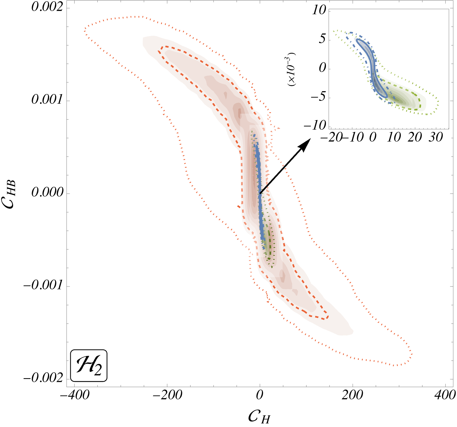
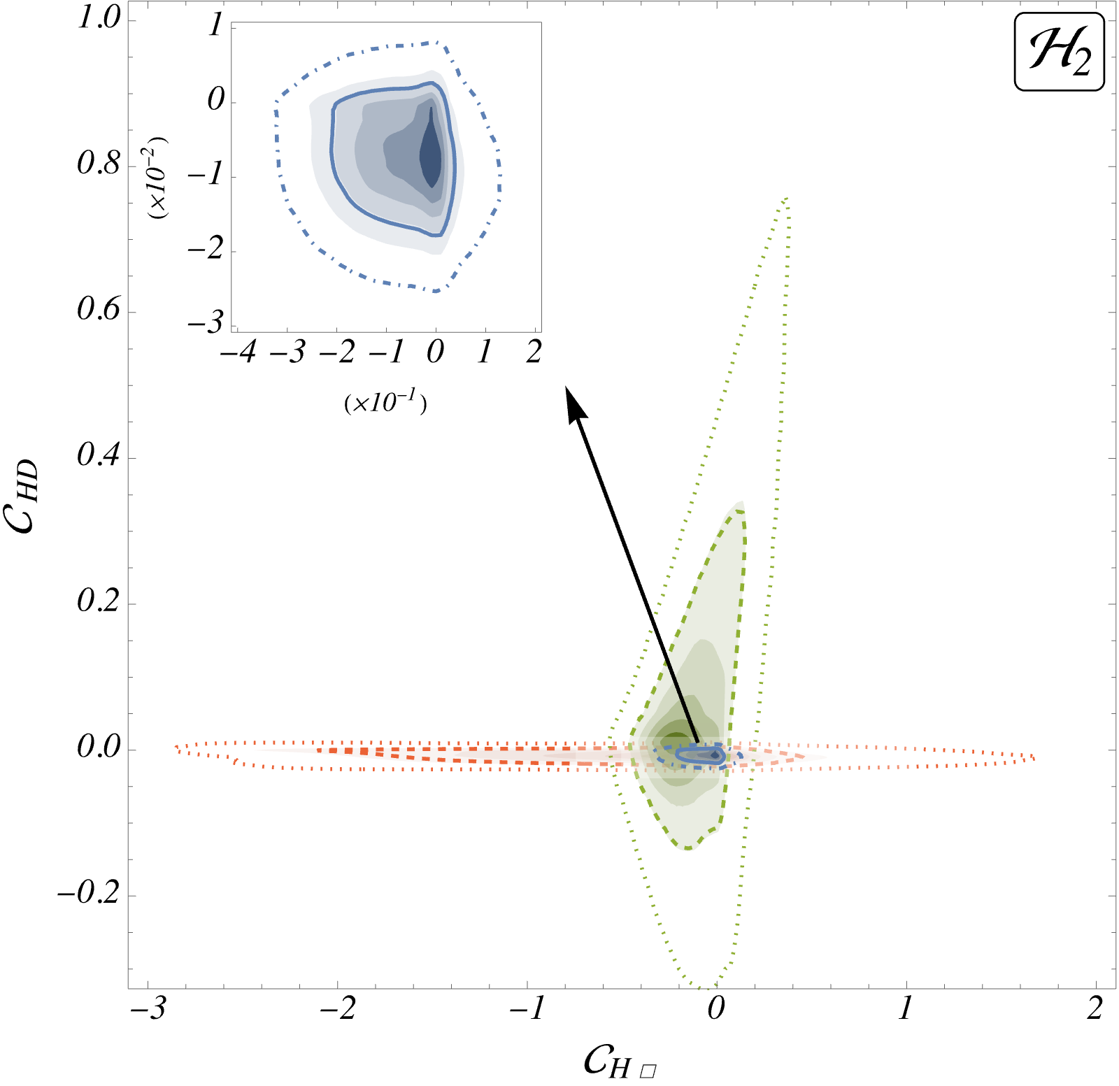
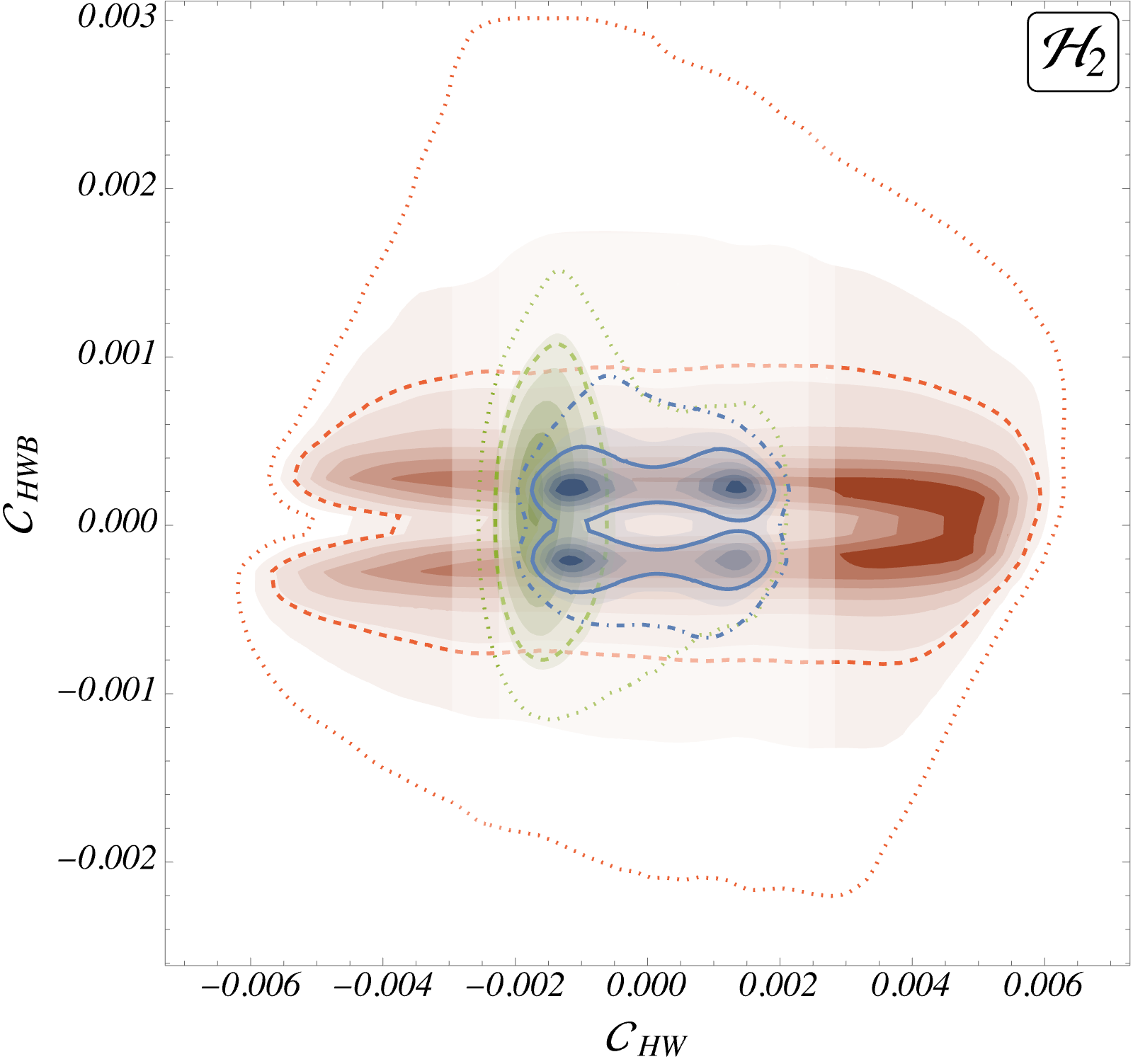
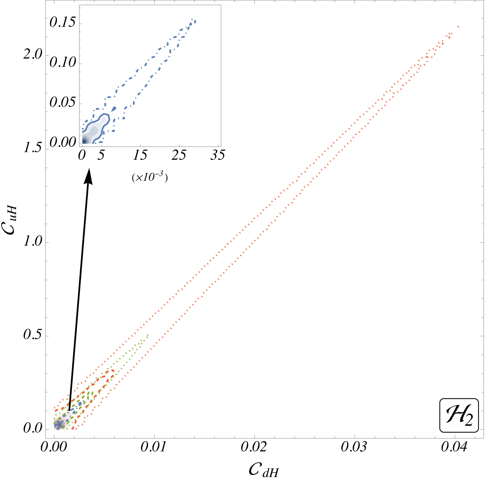
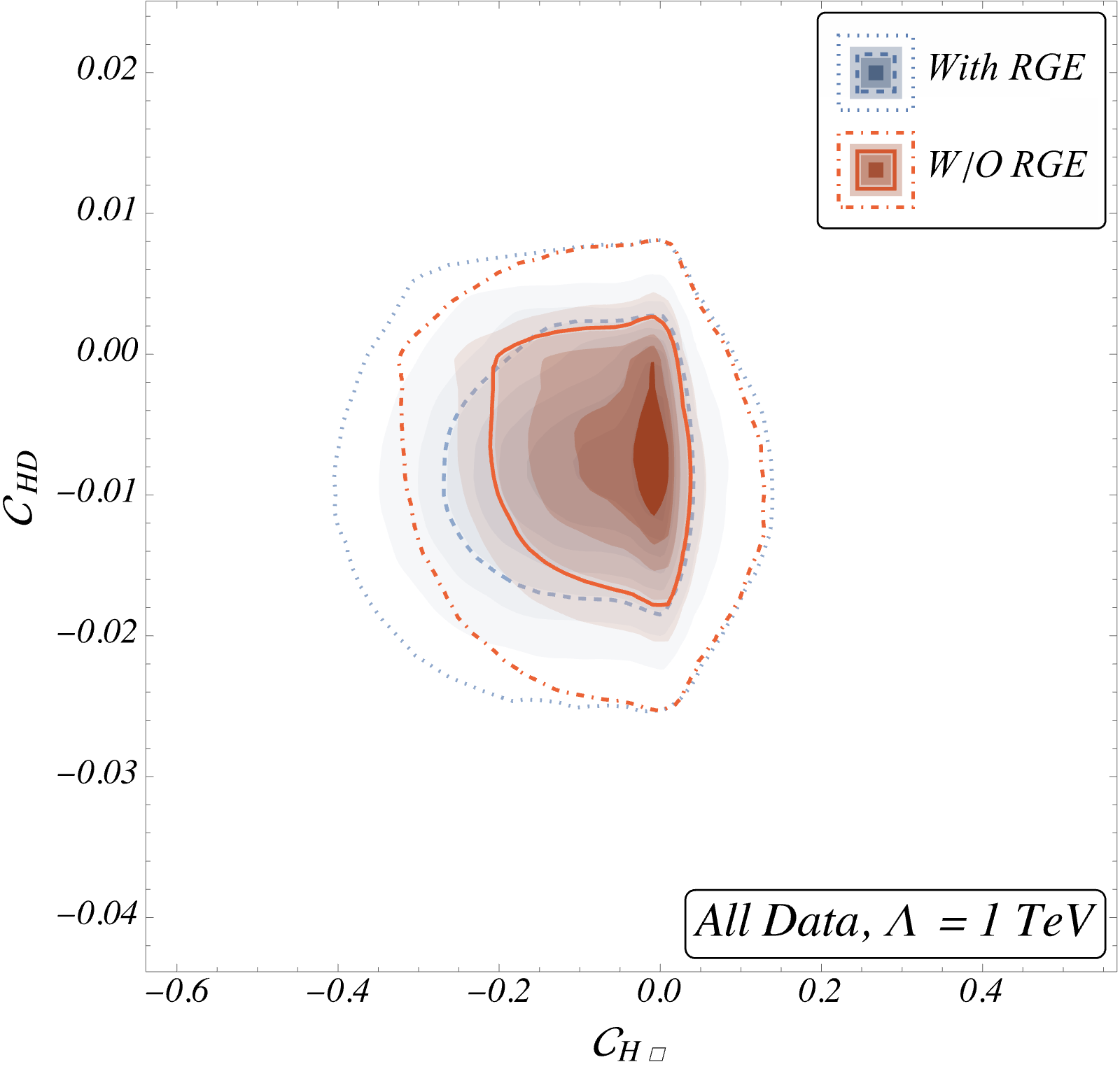
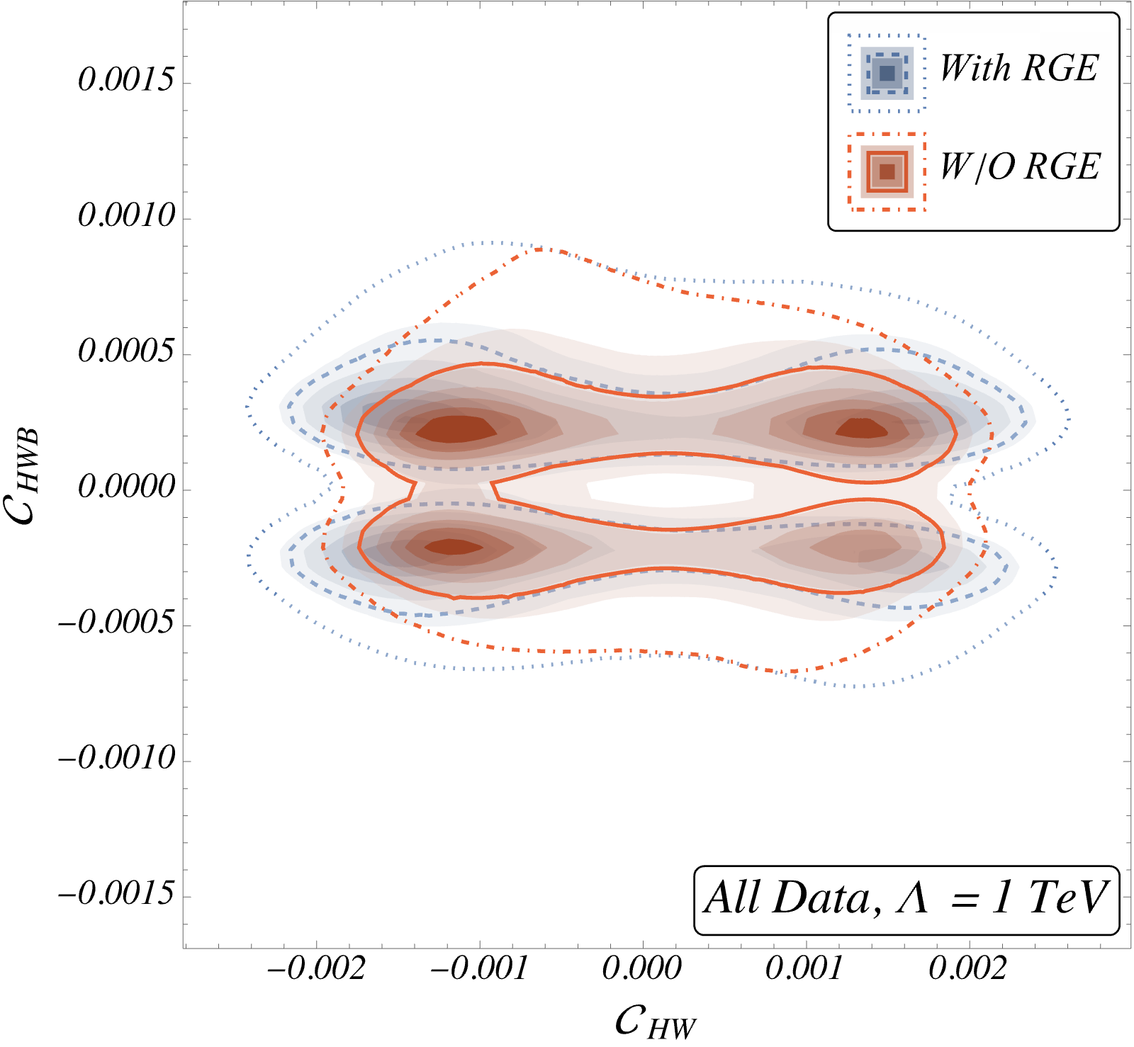
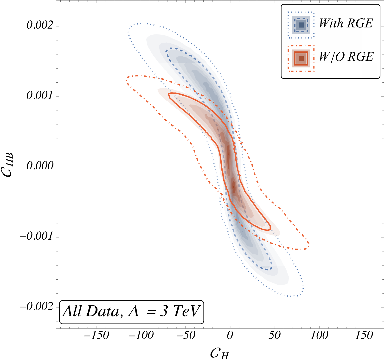
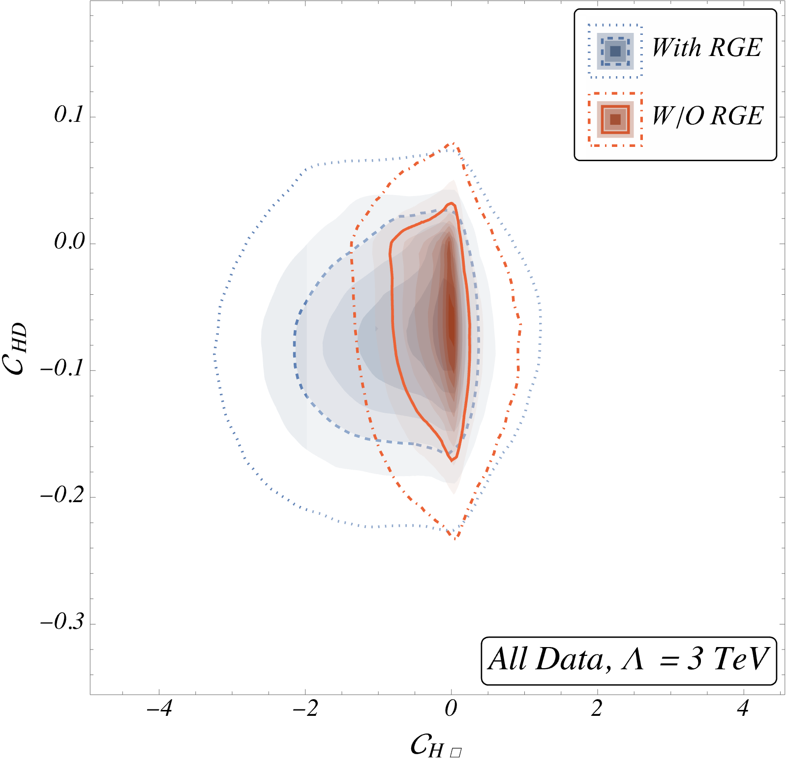
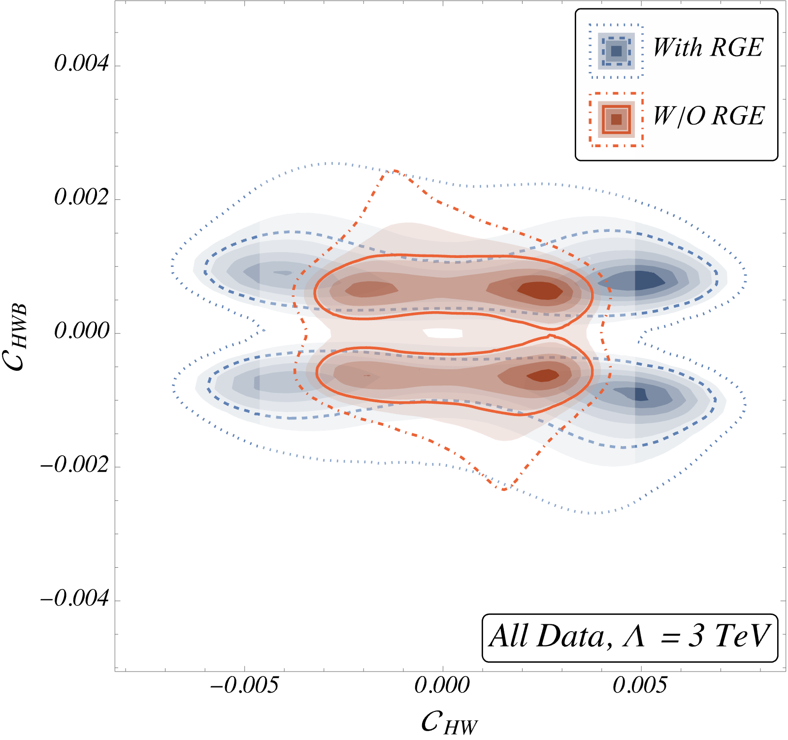
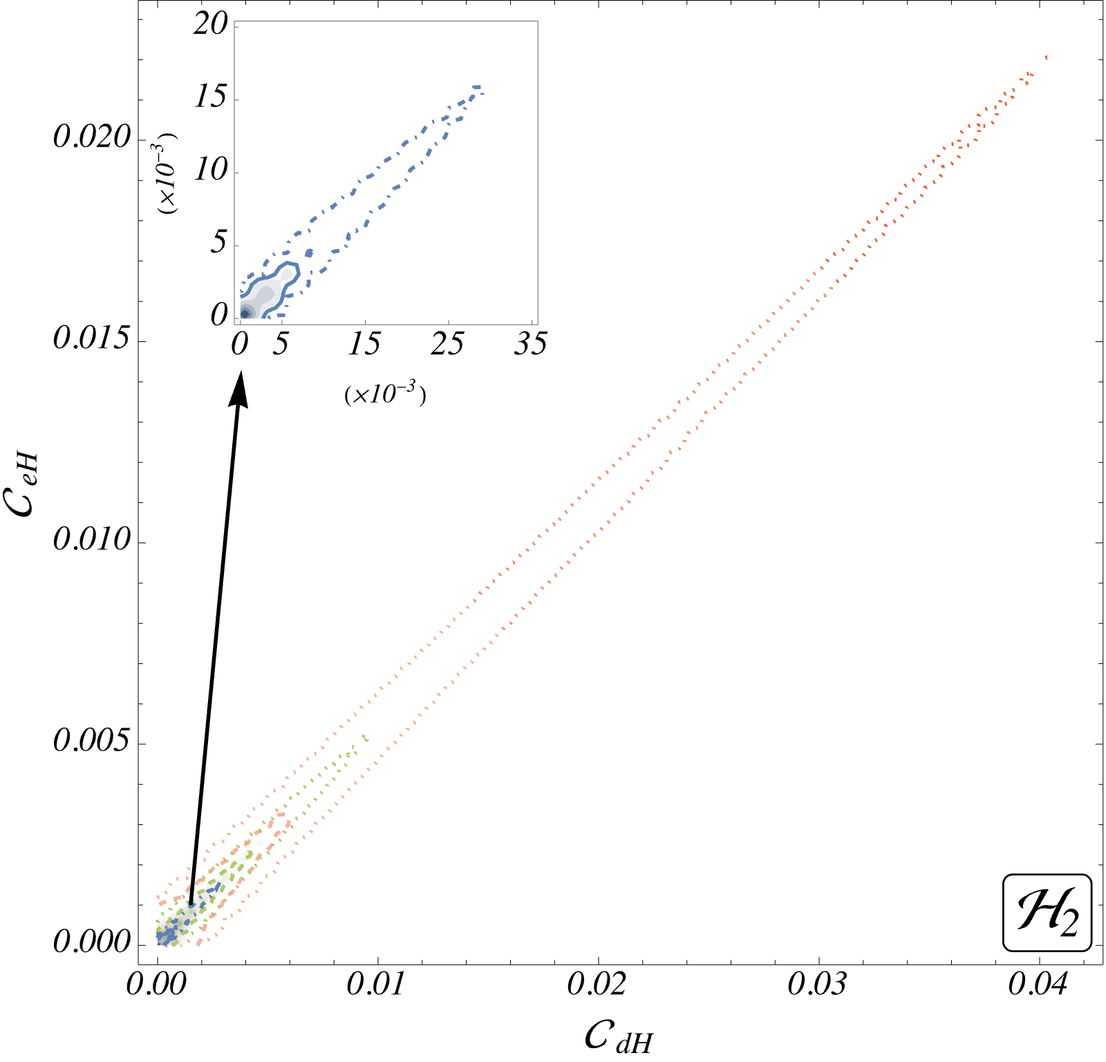
Figure 6: Two-dimensional posteriors among the relevant WCs induced by 2subscript2\mathcal{H}_{2}, listed in black in tab. 3. These regions are obtained from the parameter distributions among λ2,1subscript𝜆subscript21\lambda_{\mathcal{H}_{2},1}, λ2,2subscript𝜆subscript22\lambda_{\mathcal{H}_{2},2} and λ2,3subscript𝜆subscript23\lambda_{\mathcal{H}_{2},3} shown in figs. 5a-5c. The line contours represent the 68% and 95% CIs and the filled contours with changing opacity denote the high-probability regions with decreasing probabilities (darker to lighter). We separate the results from fitting “EWPO” data only (red), “Higgs” data only (green) and “All” data (blue).

We integrate out the heavy BSM fields up to 1-loop and tabulate the complete sets of emerging effective operators and accompanying WCs including the heavy-light mixing contribution from scalars in the loops. It is important to note that only those BSMs generate heavy-light mixed WCs in which the heavy field couples to SM fields linearly delAguila:2016zcb ; Henning:2016lyp ; Zhang:2016pja ; Ellis:2017jns ; DasBakshi:2020pbf 444A detailed discussion on the heavy-light effective action formulae is given in App. A.2.. This can be visualised by considering one-particle-irreducible 1-loop diagrams where loop propagators are both heavy and light (SM) fields, but external legs are only light (SM) fields. We further employ the equations of motion, Fierz identities, and integration by parts suitably to ensure the emergence of the exhaustive lists of effective operators up to 1-loop 555In Ref. DasBakshi:2020pbf , the effective operators are tagged as per their dominant emergence through tree (T), only heavy (HH), and heavy-light (HL) mixing.. The effective operators are depicted in the Warsaw basis Grzadkowski:2010es . The complete matching results can also be downloaded from the GitHub repository Githubresult where the readers will find the operators and the associated WCs in SILH basis as well for all these BSM scenarios. We require the Wilson coefficients of Warsaw basis effective operators in this analysis, because the observables are parameterised in terms of the SMEFT Warsaw basis operators to perform the global and the model-specific fits. The complete SMEFT dimension-six matching results for some of the SM extensions are already available in literature in Warsaw basis, for example for the real singlet scalar model Haisch:2020ahr ; Jiang:2018pbd ; Cohen:2020fcu , and scalar leptoquarks Gherardi:2020qhc . However, for the remaining models, to the best of our knowledge, the complete SMEFT dimension-six matching results in the Warsaw basis up to 1-loop including heavy-light mixing are not available yet. A tree-level matching dictionary deBlas:2017xtg , and partial results for some models including scalar heavy-light mixing (in SILH basis) Henning:2014wua ; Zhang:2016pja ; Ellis:2016enq are available as well.
Refer to caption
(a) 𝒞dHsubscript𝒞𝑑𝐻\mathcal{C}_{dH} - 𝒞eHsubscript𝒞𝑒𝐻\mathcal{C}_{eH}
Refer to caption
(b) 𝒞Hsubscript𝒞𝐻\mathcal{C}_{H} - 𝒞HBsubscript𝒞𝐻𝐵\mathcal{C}_{HB}
Refer to caption
(c) 𝒞Hsubscript𝒞𝐻\mathcal{C}_{H\square} - 𝒞HDsubscript𝒞𝐻𝐷\mathcal{C}_{HD}
Refer to caption
(d) 𝒞HWsubscript𝒞𝐻𝑊\mathcal{C}_{HW} - 𝒞HWBsubscript𝒞𝐻𝑊𝐵\mathcal{C}_{HWB}
Refer to caption
(e) 𝒞dHsubscript𝒞𝑑𝐻\mathcal{C}_{dH} - 𝒞uHsubscript𝒞𝑢𝐻\mathcal{C}_{uH}
Refer to caption
(f) Legend
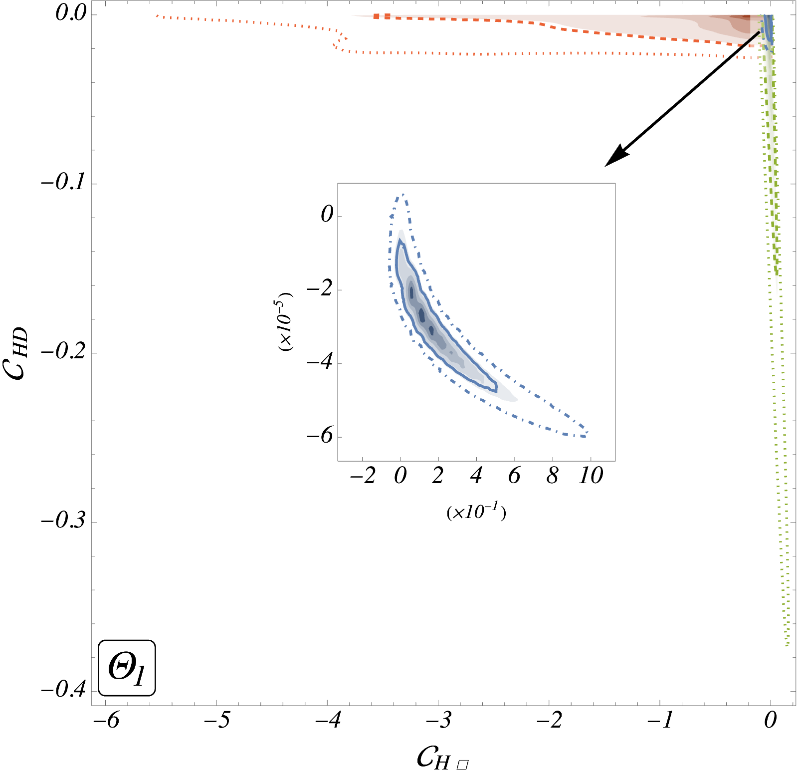
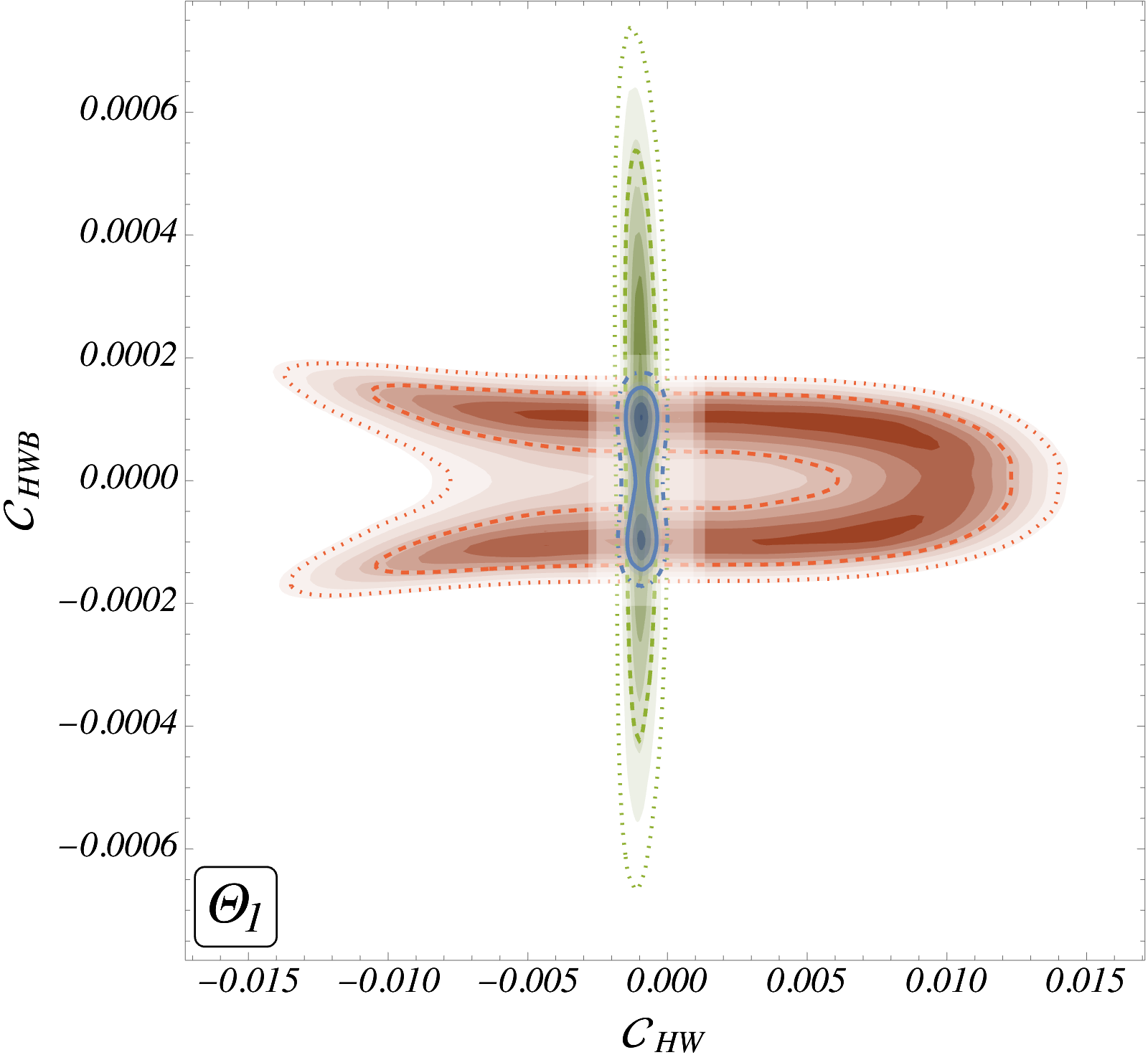
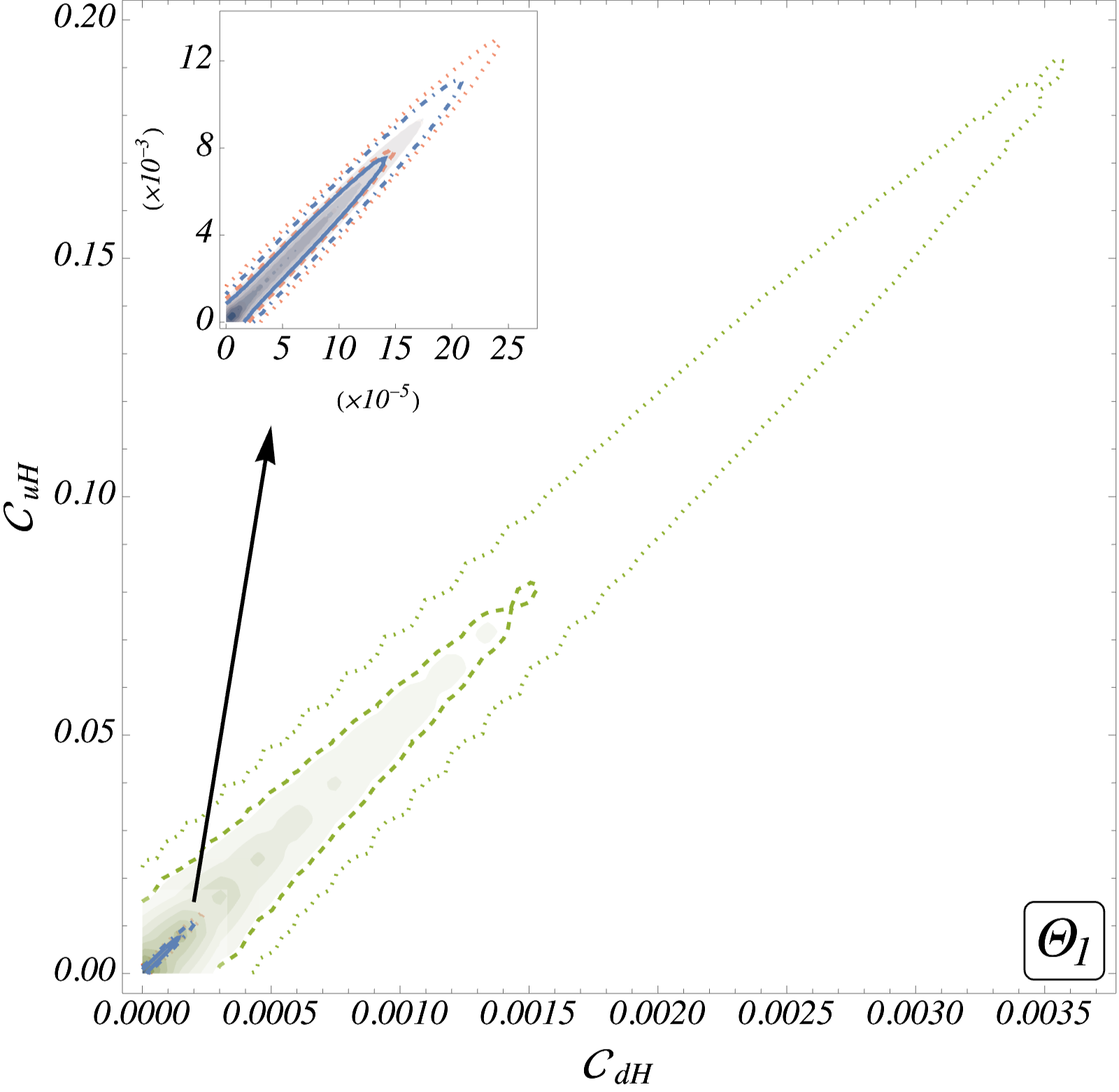
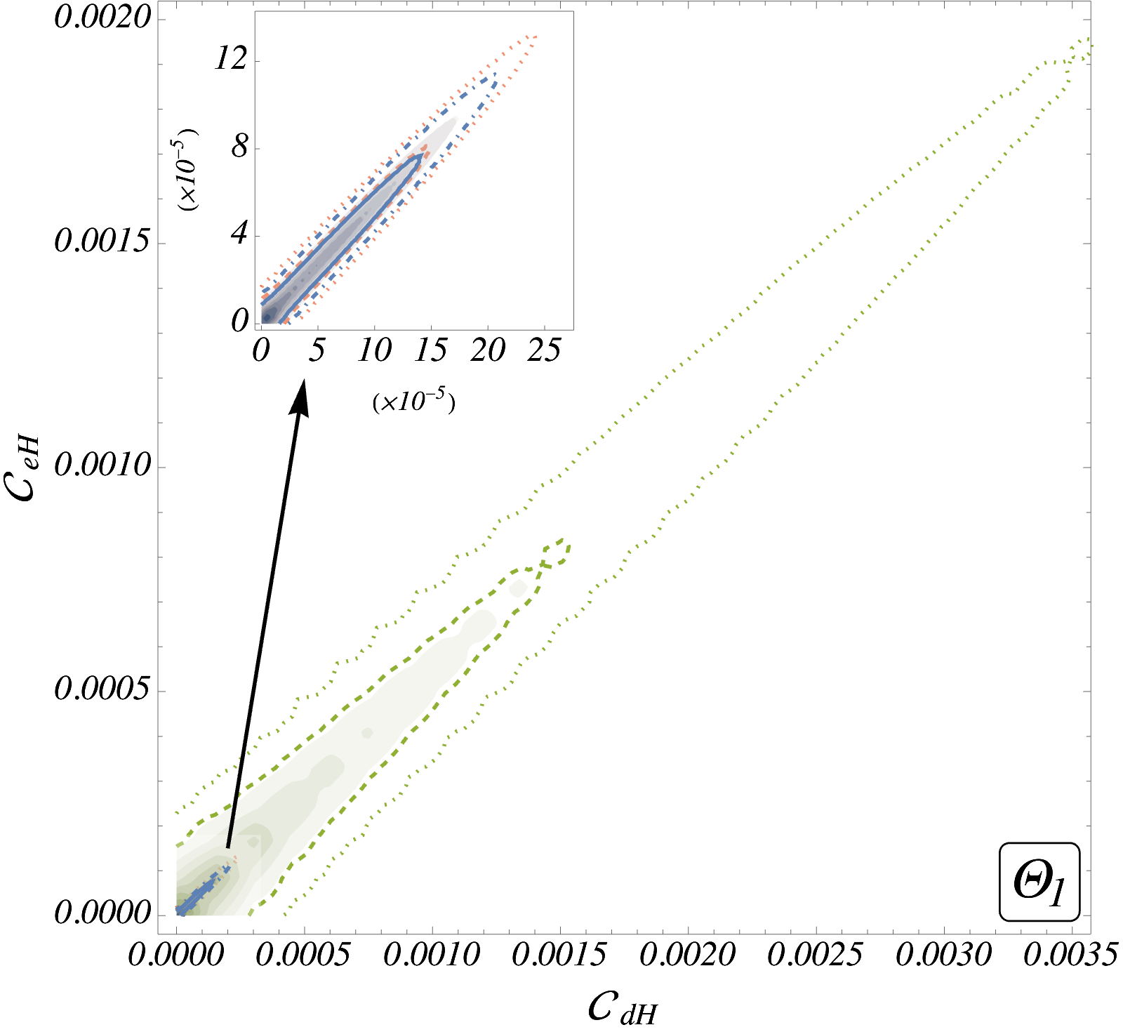
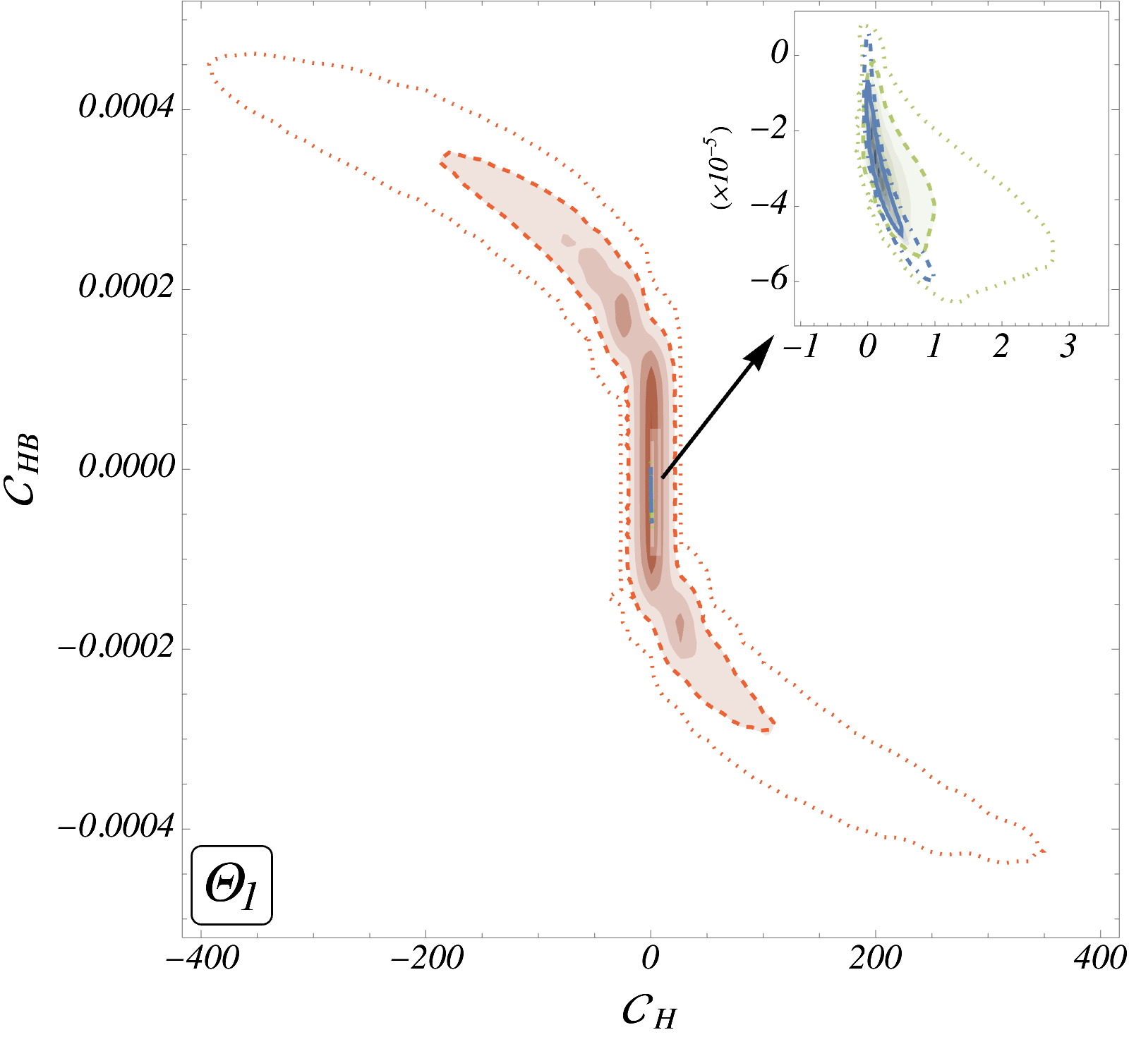
Figure 7: Two-dimensional WC posteriors, similar to fig. 6, obtained from the parameter distributions of ηΘ1(1),ηΘ1(2)superscriptsubscript𝜂subscriptΘ11superscriptsubscript𝜂subscriptΘ12\eta_{\Theta_{1}}^{(1)},\;\eta_{\Theta_{1}}^{(2)} for Θ1subscriptΘ1\Theta_{1}.

In the following subsections, we tabulate the effective operators generated and the associated WCs in terms of the model parameters in the Warsaw basis for two representative cases: The two Higgs doublet model, 2subscript2\mathcal{H}_{2}, and a scalar leptoquark, Θ1subscriptΘ1\Theta_{1}. These models encapsulate the individual features of a colour singlet and a non-singlet heavy field, respectively. The two models share the exact same set of relevant 666In our analysis, the operators which are present in our chosen set of observables and are functions of BSM parameters, are relevant. In the result section, we focus on those primarily. effective operators apart from the additional emergence of QHGsubscript𝑄HGQ_{\text{HG}} in the latter model, see tab. 4. We tabulate the results for rest of the adopted scenarios in appendix B.

Here, we provide the operators at the scale where they emerge, i.e. the cut-off scale (Λ)Λ(\Lambda) which we take equal to the mass of heavy BSM fields (mhfsubscript𝑚𝑓m_{hf}), in all cases that we discuss. We further assume that the mass of the heavy field mhfmuch-greater-thansubscript𝑚𝑓absentm_{hf}\gg EWSB scale. Thus, the heavy fields can be integrated out safely, validating the notion of EFT and all the dimension-6 operators are suppressed by 1/mhf21superscriptsubscript𝑚𝑓21/m_{hf}^{2}. Here, to start with we ignore the running of the effective operators and perform the analysis. Later, in section 6 we for extra Electro-Weak Doublet Scalar(EWDS) scenario, we discuss how the inclusion of running of effective operators leave an impact of parameter space.

In the model-independent analysis in section 4, we introduce an explicit flavour dependence for the operators of the ψ2ϕ3superscript𝜓2superscriptitalic-ϕ3\psi^{2}\phi^{3} class with the corresponding WCs QμHsubscript𝑄𝜇𝐻Q_{\mu H}, QτHsubscript𝑄𝜏𝐻Q_{\tau H}, QcHsubscript𝑄𝑐𝐻Q_{cH}, QbHsubscript𝑄𝑏𝐻Q_{bH}, and QtHsubscript𝑄𝑡𝐻Q_{tH}. As we are using CoDEx results for the model-dependent part of the analysis and CoDEx does not differentiate between flavours (yet), 𝒞μHsubscript𝒞𝜇𝐻\mathcal{C}_{\mu H} and 𝒞cHsubscript𝒞𝑐𝐻\mathcal{C}_{cH} are set to be zero for the rest of the analysis and we work with operators consisting of third generation fermions only. For the rest of the paper, the associated WCs will be denoted as 𝒞uHsubscript𝒞𝑢𝐻\mathcal{C}_{uH}, 𝒞dHsubscript𝒞𝑑𝐻\mathcal{C}_{dH}, and 𝒞eHsubscript𝒞𝑒𝐻\mathcal{C}_{eH}. In the later subsections, we highlight the operators (in red) that do not affect our chosen set of observables and thus are absent from our analysis. The blue coloured operators are functions of SM parameters only and thus, independent of our fit-parameters. Each of the observables can be thought of as a set of effective operators which has been useful to classify different single scalar field extensions of the SM DasBakshi:2020pbf . Relying on that concept, we design the methodology of our analysis to pin down the individual and mutual status of these BSM scenarios in this section.

In section 4, we obtain the constraints on the set of 23 SMEFT WCs in a model-independent manner, using the observables listed in section 3. In this section, we move a step ahead and connect the relevant observables expressed in terms of the SMEFT dimension-6 operators and their respective WCs to the BSM model parameters. The SMEFT matching results obtained for a particular BSM, mentioned above, allow us to write the WCs in terms of the respective model parameters and mhfsubscript𝑚𝑓m_{hf}. Consequently, the bounds on the model parameters of specific BSMs are obtained directly from the relevant experimental data.

The methodology of the statistical analysis is similar to the one discussed in the model-independent part. Fits are performed over the relevant BSM parameters while considering the best-fit values for the SM ones, see eq. (3). Uniform priors within range {50,50}5050\{-50,50\} are chosen for these non-SM parameters and mhfsubscript𝑚𝑓m_{hf} is chosen as to be 1 TeV uniformly in this analysis. The following subsections showcase two example scenarios where the SM is extended by two scalars, 2subscript2\mathcal{H}_{2} and Θ1subscriptΘ1\Theta_{1}, based upon the relations among the associated WCs of the emerged effective operators through the model parameters for individual cases.

5.1 Extra EW Doublet Scalar: 2(1C,2L,12|Y)subscript2subscript1𝐶subscript2𝐿evaluated-at12𝑌\mathcal{H}_{2}\equiv(1_{C},2_{L},\left.-\frac{1}{2}\right|_{Y})

This model contains an extra isospin-doublet scalar (2)subscript2(\mathcal{H}_{2}) which is a colour-singlet with hypercharge Y=12𝑌12Y=-\frac{1}{2}. The BSM Lagrangian is given as Deshpande:1977rw ; Henning:2014wua ; Nie_1999 ; Branchina:2018qlf ; Pilaftsis:1999qt ; Gunion:2002zf ,

2subscriptsubscript2\displaystyle\mathcal{L}_{\mathcal{H}_{2}} =SMd4+|𝒟μ2|2m22|2|2λ24|2|4(ηH|H~|2+η2|2|2)(H~2+2H~)absentsuperscriptsubscriptSM𝑑4superscriptsubscript𝒟𝜇subscript22superscriptsubscript𝑚subscript22superscriptsubscript22subscript𝜆subscript24superscriptsubscript24subscript𝜂𝐻superscript~𝐻2subscript𝜂subscript2superscriptsubscript22superscript~𝐻subscript2superscriptsubscript2~𝐻\displaystyle=\mathcal{L}_{{}_{\text{SM}}}^{d\leq 4}\;+|\mathcal{D}_{\mu}\mathcal{H}_{2}|^{2}-m_{\mathcal{H}_{2}}^{2}|\mathcal{H}_{2}|^{2}-\ \frac{\lambda_{\mathcal{H}_{2}}}{4}|\mathcal{H}_{2}|^{4}-(\eta_{H}|\widetilde{H}|^{2}+\eta_{\mathcal{H}_{2}}|\mathcal{H}_{2}|^{2})(\widetilde{H}^{\dagger}\mathcal{H}_{2}+\mathcal{H}_{2}^{\dagger}\widetilde{H})
λ2,1|H~|2|2|2λ2,2|H~2|2λ2,3[(H~2)2+(2H~)2]subscript𝜆subscript21superscript~𝐻2superscriptsubscript22subscript𝜆subscript22superscriptsuperscript~𝐻subscript22subscript𝜆subscript23delimited-[]superscriptsuperscript~𝐻subscript22superscriptsuperscriptsubscript2~𝐻2\displaystyle-\lambda_{\mathcal{H}_{2},1}|\widetilde{H}|^{2}|\mathcal{H}_{2}|^{2}-\lambda_{\mathcal{H}_{2},2}|\widetilde{H}^{\dagger}\mathcal{H}_{2}|^{2}-\lambda_{\mathcal{H}_{2},3}\left[(\widetilde{H}^{\dagger}\mathcal{H}_{2})^{2}+(\mathcal{H}_{2}^{\dagger}\widetilde{H})^{2}\right]
{Y2(e)l¯L~2eR+Y2(u)q¯L2uR+Y2(d)q¯L~2dR+h.c.}.subscriptsuperscript𝑌𝑒subscript2subscript¯𝑙𝐿subscript~2subscript𝑒𝑅subscriptsuperscript𝑌𝑢subscript2subscript¯𝑞𝐿subscript2subscript𝑢𝑅subscriptsuperscript𝑌𝑑subscript2subscript¯𝑞𝐿subscript~2subscript𝑑𝑅h.c.\displaystyle-\left\{Y^{(e)}_{\mathcal{H}_{2}}\overline{l}_{L}\,\widetilde{\mathcal{H}}_{2}\,e_{R}+Y^{(u)}_{\mathcal{H}_{2}}\overline{q}_{L}\,\mathcal{H}_{2}\,u_{R}+Y^{(d)}_{\mathcal{H}_{2}}\overline{q}_{L}\,\widetilde{\mathcal{H}}_{2}\,d_{R}+\text{h.c.}\right\}. (10)

Here, m2subscript𝑚subscript2m_{\mathcal{H}_{2}} is the mass of the heavy field and serves as the cut-off scale. We assume that the heavy Higgs doublet is decoupled to the SM one, and they do not mix Gunion:2002zf . This model contains nine BSM parameters ηH,η2,λ2subscript𝜂𝐻subscript𝜂subscript2subscript𝜆subscript2\eta_{H},\;\eta_{\mathcal{H}_{2}},\;\lambda_{\mathcal{H}_{2}}, λ2,1,λ2,2,λ2,3,Y2(u)subscript𝜆subscript21subscript𝜆subscript22subscript𝜆subscript23subscriptsuperscript𝑌𝑢subscript2\lambda_{\mathcal{H}_{2},1},\;\lambda_{\mathcal{H}_{2},2},\;\lambda_{\mathcal{H}_{2},3},\;Y^{(u)}_{\mathcal{H}_{2}},  Y2(d)subscriptsuperscript𝑌𝑑subscript2Y^{(d)}_{\mathcal{H}_{2}},  Y2(e)subscriptsuperscript𝑌𝑒subscript2Y^{(e)}_{\mathcal{H}_{2}}, and the WCs are functions of all these parameters along with the SM ones, see tab. 3. We assume that the BSM Yukawas couple only to the third generation of fermions. In the decoupling limit, these Yukawas do not mix with the SM ones Gunion:2002zf . We further note that the WCs of the relevant operators QuHsubscript𝑄uHQ_{\text{uH}}, QdHsubscript𝑄dHQ_{\text{dH}}, QeHsubscript𝑄eHQ_{\text{eH}}, QHsubscript𝑄HQ_{\text{H}}, QHWsubscript𝑄HWQ_{\text{HW}}, QHBsubscript𝑄HBQ_{\text{HB}}, QHWBsubscript𝑄HWBQ_{\text{HWB}}, QHsubscript𝑄HQ_{\text{H}\square}, and QHDsubscript𝑄𝐻𝐷Q_{HD} contain all the BSM parameters. In our numerical analysis, we choose to work with a Z2subscript𝑍2Z_{2}-invariant (HH𝐻𝐻H\rightarrow H and 22subscript2subscript2\mathcal{H}_{2}\rightarrow-\mathcal{H}_{2}) BSM Lagrangian. Thus the quartic couplings ηH,η2subscript𝜂𝐻subscript𝜂subscript2\eta_{H},\;\eta_{\mathcal{H}_{2}} and the Yukawa couplings Y2(u)subscriptsuperscript𝑌𝑢subscript2Y^{(u)}_{\mathcal{H}_{2}},  Y2(d)subscriptsuperscript𝑌𝑑subscript2Y^{(d)}_{\mathcal{H}_{2}},  Y2(e)subscriptsuperscript𝑌𝑒subscript2Y^{(e)}_{\mathcal{H}_{2}} couplings do not appear in our analysis, where the rest of the three parameters get constrained by our chosen experimental data set. Note that though λ2subscript𝜆subscript2\lambda_{\mathcal{H}_{2}} corresponds to Z2subscript𝑍2Z_{2} invariant term, but it still cannot be constrained as it appears in the WCs with the Z2subscript𝑍2Z_{2} violating couplings, always. Thus, to constrain these unconstrained couplings of the EWDS model, one needs to look for observables beyond the chosen ones in this work that get corrections from the following operators: Qlesubscript𝑄leQ_{\text{le}}, Qqd(1)Q_{\text{qd}}{}^{(1)}, Qqu(1)Q_{\text{qu}}{}^{(1)}, Qqu(1)Q_{\text{qu}}{}^{(1)}, Qquqd(1)Q_{\text{quqd}}{}^{(1)}, Qlequ(1)Q_{\text{lequ}}{}^{(1)}, Qledqsubscript𝑄ledqQ_{\text{ledq}}, see tab. 3. These additional observables will be helpful to constrain λ2subscript𝜆subscript2\lambda_{\mathcal{H}_{2}} even for the Z2subscript𝑍2Z_{2} symmetric Lagrangian. We need to keep in mind that the choice of the new set of observables is guided by the structures of the unconstrained WCs of this particular model only.

Constraints on the model parameters

Using the relations listed in tab. 3, we obtain the constraints on the BSM parameters directly from the experimental data. The relevant BSM fit parameters for this model are λ2,1,λ2,2subscript𝜆subscript21subscript𝜆subscript22\lambda_{\mathcal{H}_{2},1},\;\lambda_{\mathcal{H}_{2},2} and λ2,3subscript𝜆subscript23\lambda_{\mathcal{H}_{2},3} with the mass of the heavy doublet, mhfsubscript𝑚𝑓m_{hf} (cut-off scale), set to 1 TeV. The list of the dimension-6 operators coloured in black and blue in tab. 3 are replaced by the corresponding WCs in the SMEFT parameterisation of the observables. The WCs for the operators in blue are functions of only SM parameters (inputs given in eq. (3)). Those for operators in black are functions of the relevant BSM parameters and are thus relevant in constraining them. Uniform distributions within the range {50,50}5050\{-50,50\} are chosen as priors for these BSM couplings.

Using the samples from the un-normalised posteriors, we show the correlations between various BSM parameters in fig. 5 as high-probability contours of two dimensional marginal posteriors. Constant-probability-contours enclose respectively 68%percent6868\% (black solid, red/blue dashed) and 95%percent9595\% (black dot-dashed, red/blue dotted) credible regions. We also show coloured regions with variable-density-contour-shading (black/red/blue) pointing to regions of high-probability. These regions are significant to adjudge the different high-probability regions in the allowed parameter space. This is evident from the posteriors obtained from the “All” measurements fit, which contain more than one high-probability region. For instance, in fig. 5a, there are four different high-probability regions within the 68%percent6868\% credible region enclosed by the solid black constant-probability-contour.

In order to demonstrate the constraining power of different datasets, in the top row of the fig. 5, the posterior distributions of these three parameters obtained are shown from “All” (black), “Higgs” (red) and “EWPO” (blue) sets of experimental measurements. While the constraints from Higgs data are overall a bit stronger, EWPO data add orthogonal information, leading to significantly tightened bounds when combining the data from both sectors. In fig. 5a, the bound on λ2,1subscript𝜆subscript21\lambda_{\mathcal{H}_{2},1} from EWPO only is very relaxed as compared to the others. This happens primarily because in case of EWPO, λ2,1subscript𝜆subscript21\lambda_{\mathcal{H}_{2},1} gets constrained through QHsubscript𝑄𝐻Q_{H} only whose contribution appears at two-loop in the SMEFT parameterisation of mWsubscript𝑚𝑊m_{W} and is very small. For other datasets on the other hand, λ2,1subscript𝜆subscript21\lambda_{\mathcal{H}_{2},1} gets bounded from other operators QHsubscript𝑄𝐻Q_{H\square}, QHBsubscript𝑄𝐻𝐵Q_{HB}, QHWsubscript𝑄𝐻𝑊Q_{HW} besides QHsubscript𝑄𝐻Q_{H}. The corresponding WCs receive strong constraints from Higgs signal strengths and in particular from di-Higgs data, as depicted by the corresponding parameter spaces.

Model-Dependent constraints on the WCs

As mentioned in the beginning of this section, we take our model-independent analysis in sec. 4 to the next step, by determining the allowed WC spaces for specific models, using their parameter-posteriors and the WC matching results obtained after integrating out the heavy BSM particle. In this case, the matched WCs are functions of BSM parameters and dependent on one another. The WC-spaces obtained in this way are directed from the constraints of the relevant model parameters and thus are termed as “model-dependent”. Using the large MCMC samples generated from the model-parameter-posterior, we generate the multi-variate distributions of those WCs (now functions of model parameters). We show these distributions in the WC-space with the help of marginal-posteriors of two WCs at a time.

For 2subscript2\mathcal{H}_{2}, we generate the distributions of the WCs (black) using relations (obtained after matching) from tab. 3 expressed in terms of parameters: λ2,1,λ2,2subscript𝜆subscript21subscript𝜆subscript22\lambda_{\mathcal{H}_{2},1},\;\lambda_{\mathcal{H}_{2},2} and λ2,3subscript𝜆subscript23\lambda_{\mathcal{H}_{2},3}, and propagating the model-parameter-posteriors. As before, we demonstrate the relative effects of different datasets named “All”, “EWPO”, and “Higgs” separately. Instead of showing all the possible 2D-marginal contour-plots for the WCs, we choose to show a few sample plots in fig. 6.

Solid blue (dashed red/green) constant-probability-contours enclose the 68%percent6868\% and dot-dashed blue (dotted red/green) ones enclose the 95%percent9595\% credible regions, respectively. Coloured regions (blue/red/green) with variable density depict the high probability regions. In some cases, the parameter spaces obtained for the three datasets differ from one another by order(s) of magnitude. For instance, the bluish regions corresponding to “All” measurements are imperceptibly tiny in comparison to those corresponding to both the “EWPO” (red) and “Higgs” (green) datasets. For ease of viewing, we have magnified such regions and shown them as insets.

As mentioned earlier, these obtained WC-spaces are related by non-linear relations of the model parameters. This is explicitly illustrated from the WC-expressions for 𝒞dHsubscript𝒞𝑑𝐻\mathcal{C}_{dH}, 𝒞eHsubscript𝒞𝑒𝐻\mathcal{C}_{eH} and 𝒞uHsubscript𝒞𝑢𝐻\mathcal{C}_{uH} in tab. 3 which, after taking the contributions from the relevant BSM parameters, turn out to be positive definite. As a result, the corresponding parameter spaces shown in figs. 6a and 6e are delimited only in the positive quadrant.

5.2 Scalar Leptoquark: Θ1(3C,2L,16|Y)subscriptΘ1subscript3𝐶subscript2𝐿evaluated-at16𝑌\Theta_{1}\equiv(3_{C},2_{L},\left.\frac{1}{6}\right|_{Y})

In this model, we extend the SM by a colour-triplet isospin-doublet scalar (Θ1subscriptΘ1\Theta_{1}) with hypercharge Y=16𝑌16Y=\frac{1}{6}. We consider the BSM Lagrangian Buchmuller:1986zs ; Arnold:2013cva ,

Θ1subscriptsubscriptΘ1\displaystyle\mathcal{L}_{\Theta_{1}} =SMd4+(DμΘ1)(DμΘ1)mΘ12Θ1Θ1ηΘ1(1)HHΘ1Θ1ηΘ1(2)(HσiH)(Θ1σiΘ1)absentsuperscriptsubscriptSM𝑑4superscriptsubscript𝐷𝜇subscriptΘ1superscript𝐷𝜇subscriptΘ1superscriptsubscript𝑚subscriptΘ12superscriptsubscriptΘ1subscriptΘ1superscriptsubscript𝜂subscriptΘ11superscript𝐻𝐻superscriptsubscriptΘ1subscriptΘ1superscriptsubscript𝜂subscriptΘ12superscript𝐻superscript𝜎𝑖𝐻superscriptsubscriptΘ1superscript𝜎𝑖subscriptΘ1\displaystyle=\mathcal{L}_{{}_{\text{SM}}}^{d\leq 4}\;+\left(D_{\mu}\Theta_{1}\right)^{\dagger}\,\left(D^{\mu}\Theta_{1}\right)-m_{{\Theta_{1}}}^{2}\,\Theta_{1}^{\dagger}\Theta_{1}-\eta_{{}_{\Theta_{1}}}^{(1)}H^{\dagger}H\,\Theta_{1}^{\dagger}\Theta_{1}-\eta_{{}_{\Theta_{1}}}^{(2)}\left(H^{\dagger}\sigma^{i}H\right)\,\left(\Theta_{1}^{\dagger}\sigma^{i}\Theta_{1}\right)
λΘ1(1)(Θ1Θ1)2λΘ1(2)(Θ1σiΘ1)2+{yΘ1Θ1αd¯Rαiσ2lL+h.c.}.superscriptsubscript𝜆subscriptΘ11superscriptsuperscriptsubscriptΘ1subscriptΘ12superscriptsubscript𝜆subscriptΘ12superscriptsuperscriptsubscriptΘ1superscript𝜎𝑖subscriptΘ12subscript𝑦subscriptΘ1superscriptsubscriptΘ1𝛼superscriptsubscript¯𝑑𝑅𝛼𝑖superscript𝜎2subscript𝑙𝐿h.c.\displaystyle-\lambda_{\Theta_{1}}^{(1)}\left(\Theta_{1}^{\dagger}\Theta_{1}\right)^{2}-\lambda_{\Theta_{1}}^{(2)}\left(\Theta_{1}^{\dagger}\sigma^{i}\Theta_{1}\right)^{2}+\left\{y_{\Theta_{1}}\Theta_{1}^{\alpha}{\overline{d}_{R}^{\alpha}}i\sigma^{2}l_{L}+\text{h.c.}\right\}. (11)

Here, mΘ1subscript𝑚subscriptΘ1m_{\Theta_{1}} is the mass of the heavy field, i.e. the cut-off scale appears in the WCs. This model contains five BSM parameters, ηΘ1(1),ηΘ1(2),λΘ1(1),λΘ1(2)superscriptsubscript𝜂subscriptΘ11superscriptsubscript𝜂subscriptΘ12superscriptsubscript𝜆subscriptΘ11superscriptsubscript𝜆subscriptΘ12\eta_{\Theta_{1}}^{(1)},\;\eta_{\Theta_{1}}^{(2)},\;\lambda_{\Theta_{1}}^{(1)},\;\lambda_{\Theta_{1}}^{(2)}, and yΘ1subscript𝑦subscriptΘ1y_{\Theta_{1}}, and the WCs are functions of these parameters on top of the SM ones, see tab. 4. In the BSM Yukawa coupling, we assume that yΘ1subscript𝑦subscriptΘ1y_{\Theta_{1}} couples to third generation fermions only. As mentioned earlier, not all the emerged operators affect our selected observables, only QuHsubscript𝑄uHQ_{\text{uH}}, QdHsubscript𝑄dHQ_{\text{dH}}, QeHsubscript𝑄eHQ_{\text{eH}}, QHsubscript𝑄HQ_{\text{H}}, QHWsubscript𝑄HWQ_{\text{HW}}, QHBsubscript𝑄HBQ_{\text{HB}}, QHWBsubscript𝑄HWBQ_{\text{HWB}}, QHGsubscript𝑄HGQ_{\text{HG}}, QHsubscript𝑄HQ_{\text{H}\square}, and QHDsubscript𝑄HDQ_{\text{HD}} are the relevant ones for our analysis. Thus out of these five BSM parameters, only ηΘ1(1)superscriptsubscript𝜂subscriptΘ11\eta_{\Theta_{1}}^{(1)}, and ηΘ1(2)superscriptsubscript𝜂subscriptΘ12\eta_{\Theta_{1}}^{(2)} get constrained by the experimental data while the others play no role. To constrain them, we need to add more observables that get contributions from the Qldsubscript𝑄ldQ_{\text{ld}} operators, see tab. 4. Note that the unconstrained operator, that are functions of the BSM parameters, sets belonging to these example models are mutually orthogonal, the requirement of additional observables for these two scenarios also do not overlap. Thus, to constrain all the BSM parameters 777The corrections to the low-energy observables including the electric dipole moments require an enhancement in the SMEFT operator list to include multiple generations of fermions (see Refs. Falkowski:2017pss ; Dekens:2018bci ), which is beyond the scope of this paper. In this work, we concern ourselves only with flavour diagonal operators. We leave the flavour off-diagonal scenario as a future project., one may have to look for some of the observables for individual models case by case.

Constraints on the model parameters ηΘ1(1),ηΘ1(2)superscriptsubscript𝜂subscriptΘ11superscriptsubscript𝜂subscriptΘ12\eta_{\Theta_{1}}^{(1)},\;\eta_{\Theta_{1}}^{(2)}

With uniform priors within the range {50,50}5050\{-50,50\} and following the same methodology as mentioned for 2subscript2\mathcal{H}_{2}, we showcase the parameter-space of the two BSM couplings (ηΘ1(1)superscriptsubscript𝜂subscriptΘ11\eta_{\Theta_{1}}^{(1)} and ηΘ1(2)superscriptsubscript𝜂subscriptΘ12\eta_{\Theta_{1}}^{(2)}) for model Θ1subscriptΘ1\Theta_{1} as two-dimensional marginalised posteriors in fig. 5d, for the same datasets as before: “EWPO” (blue), “Higgs” (red), and “All” (black). The figure shows that the “EWPO” bound on ηΘ1(1)superscriptsubscript𝜂subscriptΘ11\eta_{\Theta_{1}}^{(1)} is the most relaxed, owing to the loop-order contribution to QHsubscript𝑄𝐻Q_{H}, whereas those allowed by “Higgs” and “All” datasets are of almost same order and have negative limits. This is because apart from QHsubscript𝑄𝐻Q_{H}, there are other operators like QHBsubscript𝑄𝐻𝐵Q_{HB}, QHsubscript𝑄𝐻Q_{H\square}, QHGsubscript𝑄𝐻𝐺Q_{HG} and QHWsubscript𝑄𝐻𝑊Q_{HW} which give relatively stronger contributions to other two datasets. In contrast, the constraints on ηΘ1(2)superscriptsubscript𝜂subscriptΘ12\eta_{\Theta_{1}}^{(2)} are the weakest from “Higgs” data and are of similar range for “EWPO” and “All”. This is a consequence of the strong contribution from QHWBsubscript𝑄𝐻𝑊𝐵Q_{HWB} and QHDsubscript𝑄𝐻𝐷Q_{HD} to “EWPO”, which is also evident for “All’ measurements.

Model-Dependent constraints on the WCs

In the next part of the analysis, similar to the case of 2subscript2\mathcal{H}_{2}, distributions are generated for the 10 WCs of the model Θ1subscriptΘ1\Theta_{1} (expressions in black in tab. 4) for the three different datasets. Similar to fig. 6, some chosen two-dimensional marginal distributions are shown in fig. 7 for Θ1subscriptΘ1\Theta_{1}. As already noted, these WC-distributions are generated from the model-parameter-posteriors (i.e. ηΘ1(1)superscriptsubscript𝜂subscriptΘ11\eta_{\Theta_{1}}^{(1)} and ηΘ1(2)superscriptsubscript𝜂subscriptΘ12\eta_{\Theta_{1}}^{(2)}), using the expressions listed in tab. 4. The WCs 𝒞eHsubscript𝒞𝑒𝐻\mathcal{C}_{eH}, 𝒞dHsubscript𝒞𝑑𝐻\mathcal{C}_{dH}, and 𝒞uHsubscript𝒞𝑢𝐻\mathcal{C}_{uH}, representing Yukawa-type interactions, are functions of the squared power of ηΘ1(2)superscriptsubscript𝜂subscriptΘ12\eta_{\Theta_{1}}^{(2)}. As a result, these WCs will only take positive values when determined in the Θ1subscriptΘ1\Theta_{1} model. This is clearly shown in 2D marginalised WC-distributions in figs. 7a and 7e. The opposite behaviour is visible in the WC-space of 𝒞HDsubscript𝒞𝐻𝐷\mathcal{C}_{HD} in the fig. 7c which yields negative limits. From fig. 5d, it is evident that the constraints for ηΘ1(1)superscriptsubscript𝜂subscriptΘ11\eta_{\Theta_{1}}^{(1)} for “Higgs” and “All” datasets have negative limits. This leads to the negative bounds on QHWsubscript𝑄𝐻𝑊Q_{HW} which is a linear function of ηΘ1(1)superscriptsubscript𝜂subscriptΘ11\eta_{\Theta_{1}}^{(1)}, as depicted in fig. 7d for the corresponding datasets.

Order-of-magnitude variations in the size of the WC-spaces between models, as shown in figs. 6 and 7, point to the significance of the SMEFT matching expressions as well as the BSM parameter-spaces in determining model-dependent WC-constraints.

Table 4: Warsaw basis effective operators and the associated WCs that emerge after integrating-out the heavy field Θ1subscriptΘ1\Theta_{1}: (3,2,1616\frac{1}{6}). See caption of tab. 3 for colour coding.
Dim-6 Ops. Wilson coefficients
QHBsubscript𝑄HBQ_{\text{HB}} gY2ηΘ1(1)1152π2mΘ12superscriptsubscript𝑔𝑌2superscriptsubscript𝜂subscriptΘ111152superscript𝜋2superscriptsubscript𝑚subscriptΘ12\frac{g_{Y}^{2}\eta_{\Theta_{1}}^{(1)}}{1152\pi^{2}m_{\Theta_{1}}^{2}}
QHsubscript𝑄𝐻Q_{H\square} gW42560π2mΘ12ηΘ1(1)232π2mΘ12+ηΘ1(2)2512π2mΘ12-\frac{g_{W}^{4}}{2560\pi^{2}m_{\Theta_{1}}^{2}}-\frac{\eta_{\Theta_{1}}^{(1)}{}^{2}}{32\pi^{2}m_{\Theta_{1}}^{2}}+\frac{\eta_{\Theta_{1}}^{(2)}{}^{2}}{512\pi^{2}m_{\Theta_{1}}^{2}}
QHDsubscript𝑄HDQ_{\text{HD}} gY45760π2mΘ12ηΘ1(2)2128π2mΘ12-\frac{g_{Y}^{4}}{5760\pi^{2}m_{\Theta_{1}}^{2}}-\frac{\eta_{\Theta_{1}}^{(2)}{}^{2}}{128\pi^{2}m_{\Theta_{1}}^{2}}
QHGsubscript𝑄HGQ_{\text{HG}} gS2ηΘ1(1)192π2mΘ12superscriptsubscript𝑔𝑆2superscriptsubscript𝜂subscriptΘ11192superscript𝜋2superscriptsubscript𝑚subscriptΘ12\frac{g_{S}^{2}\eta_{\Theta_{1}}^{(1)}}{192\pi^{2}m_{\Theta_{1}}^{2}}
QHWsubscript𝑄HWQ_{\text{HW}} gW2ηΘ1(1)128π2mΘ12superscriptsubscript𝑔𝑊2superscriptsubscript𝜂subscriptΘ11128superscript𝜋2superscriptsubscript𝑚subscriptΘ12\frac{g_{W}^{2}\eta_{\Theta_{1}}^{(1)}}{128\pi^{2}m_{\Theta_{1}}^{2}}
QHWBsubscript𝑄HWBQ_{\text{HWB}} gWgYηΘ1(2)768π2mΘ12subscript𝑔𝑊subscript𝑔𝑌superscriptsubscript𝜂subscriptΘ12768superscript𝜋2superscriptsubscript𝑚subscriptΘ12\frac{g_{W}g_{Y}\eta_{\Theta_{1}}^{(2)}}{768\pi^{2}m_{\Theta_{1}}^{2}}
QuHsubscript𝑄uHQ_{\text{uH}} ηΘ1(2)YuSM2256π2mΘ12superscriptsubscript𝜂subscriptΘ12superscriptsuperscriptsubscript𝑌𝑢SM2256superscript𝜋2superscriptsubscript𝑚subscriptΘ12\frac{\eta_{\Theta_{1}}^{(2)}{}^{2}Y_{u}^{\text{SM}}}{256\pi^{2}m_{\Theta_{1}}^{2}}
QdHsubscript𝑄dHQ_{\text{dH}} ηΘ1(2)YdSM2256π2mΘ12superscriptsubscript𝜂subscriptΘ12superscriptsuperscriptsubscript𝑌𝑑SM2256superscript𝜋2superscriptsubscript𝑚subscriptΘ12\frac{\eta_{\Theta_{1}}^{(2)}{}^{2}Y_{d}^{\text{SM}}}{256\pi^{2}m_{\Theta_{1}}^{2}}
QeHsubscript𝑄eHQ_{\text{eH}} ηΘ1(2)YeSM2256π2mΘ12superscriptsubscript𝜂subscriptΘ12superscriptsuperscriptsubscript𝑌𝑒SM2256superscript𝜋2superscriptsubscript𝑚subscriptΘ12\frac{\eta_{\Theta_{1}}^{(2)}{}^{2}Y_{e}^{\text{SM}}}{256\pi^{2}m_{\Theta_{1}}^{2}}
QHsubscript𝑄𝐻Q_{H} ηΘ1(1)316π2mΘ123ηΘ1(1)ηΘ1(2)2256π2mΘ12+ηΘ1(2)λHSM2128π2mΘ12-\frac{\eta_{\Theta_{1}}^{(1)}{}^{3}}{16\pi^{2}m_{\Theta_{1}}^{2}}-\frac{3\eta_{\Theta_{1}}^{(1)}\eta_{\Theta_{1}}^{(2)}{}^{2}}{256\pi^{2}m_{\Theta_{1}}^{2}}+\frac{\eta_{\Theta_{1}}^{(2)}{}^{2}\lambda_{H}^{\text{SM}}}{128\pi^{2}m_{\Theta_{1}}^{2}}
Qllsubscript𝑄llQ_{\text{ll}} gW42560π2mΘ12gY423040π2mΘ12superscriptsubscript𝑔𝑊42560superscript𝜋2superscriptsubscript𝑚subscriptΘ12superscriptsubscript𝑔𝑌423040superscript𝜋2superscriptsubscript𝑚subscriptΘ12-\frac{g_{W}^{4}}{2560\pi^{2}m_{\Theta_{1}}^{2}}-\frac{g_{Y}^{4}}{23040\pi^{2}m_{\Theta_{1}}^{2}}
QHl(1)Q_{\text{Hl}}{}^{(1)} gY411520π2mΘ12superscriptsubscript𝑔𝑌411520superscript𝜋2superscriptsubscript𝑚subscriptΘ12\frac{g_{Y}^{4}}{11520\pi^{2}m_{\Theta_{1}}^{2}}
QHq(1)Q_{\text{Hq}}{}^{(1)} gY434560π2mΘ12superscriptsubscript𝑔𝑌434560superscript𝜋2superscriptsubscript𝑚subscriptΘ12-\frac{g_{Y}^{4}}{34560\pi^{2}m_{\Theta_{1}}^{2}}
QHl(3)Q_{\text{Hl}}{}^{(3)} gW4640π2mΘ12superscriptsubscript𝑔𝑊4640superscript𝜋2superscriptsubscript𝑚subscriptΘ12-\frac{g_{W}^{4}}{640\pi^{2}m_{\Theta_{1}}^{2}}
QHq(3)Q_{\text{Hq}}{}^{(3)} gW4640π2mΘ12superscriptsubscript𝑔𝑊4640superscript𝜋2superscriptsubscript𝑚subscriptΘ12-\frac{g_{W}^{4}}{640\pi^{2}m_{\Theta_{1}}^{2}}
QGsubscript𝑄𝐺Q_{G} gS32880π2mΘ12superscriptsubscript𝑔𝑆32880superscript𝜋2superscriptsubscript𝑚subscriptΘ12\frac{g_{S}^{3}}{2880\pi^{2}m_{\Theta_{1}}^{2}}
QHusubscript𝑄HuQ_{\text{Hu}} gY48640π2mΘ12superscriptsubscript𝑔𝑌48640superscript𝜋2superscriptsubscript𝑚subscriptΘ12-\frac{g_{Y}^{4}}{8640\pi^{2}m_{\Theta_{1}}^{2}}
QHdsubscript𝑄HdQ_{\text{Hd}} gY417280π2mΘ12superscriptsubscript𝑔𝑌417280superscript𝜋2superscriptsubscript𝑚subscriptΘ12\frac{g_{Y}^{4}}{17280\pi^{2}m_{\Theta_{1}}^{2}}
QHesubscript𝑄HeQ_{\text{He}} gY45760π2mΘ12\frac{g_{Y}^{4}}{5760\pi^{2}m_{\Theta_{1}}{}^{2}}
QWsubscript𝑄𝑊Q_{W} gW31920π2mΘ12superscriptsubscript𝑔𝑊31920superscript𝜋2superscriptsubscript𝑚subscriptΘ12\frac{g_{W}^{3}}{1920\pi^{2}m_{\Theta_{1}}^{2}}
(a)
Dim-6 Ops. Wilson coefficients
Qlq(1)Q_{\text{lq}}{}^{(1)} gY434560π2mΘ12superscriptsubscript𝑔𝑌434560superscript𝜋2superscriptsubscript𝑚subscriptΘ12\frac{g_{Y}^{4}}{34560\pi^{2}m_{\Theta_{1}}^{2}}
Qqd(1)Q_{\text{qd}}{}^{(1)} gY451840π2mΘ12superscriptsubscript𝑔𝑌451840superscript𝜋2superscriptsubscript𝑚subscriptΘ12\frac{g_{Y}^{4}}{51840\pi^{2}m_{\Theta_{1}}^{2}}
Qqq(1)Q_{\text{qq}}{}^{(1)} gY4207360π2mΘ12superscriptsubscript𝑔𝑌4207360superscript𝜋2superscriptsubscript𝑚subscriptΘ12-\frac{g_{Y}^{4}}{207360\pi^{2}m_{\Theta_{1}}^{2}}
Qqu(1)Q_{\text{qu}}{}^{(1)} gY425920π2mΘ12superscriptsubscript𝑔𝑌425920superscript𝜋2superscriptsubscript𝑚subscriptΘ12-\frac{g_{Y}^{4}}{25920\pi^{2}m_{\Theta_{1}}^{2}}
Qud(1)Q_{\text{ud}}{}^{(1)} gY412960π2mΘ12superscriptsubscript𝑔𝑌412960superscript𝜋2superscriptsubscript𝑚subscriptΘ12\frac{g_{Y}^{4}}{12960\pi^{2}m_{\Theta_{1}}^{2}}
Qlq(3)Q_{\text{lq}}{}^{(3)} gW41280π2mΘ12superscriptsubscript𝑔𝑊41280superscript𝜋2superscriptsubscript𝑚subscriptΘ12-\frac{g_{W}^{4}}{1280\pi^{2}m_{\Theta_{1}}^{2}}
Qqq(3)Q_{\text{qq}}{}^{(3)} gW42560π2mΘ12superscriptsubscript𝑔𝑊42560superscript𝜋2superscriptsubscript𝑚subscriptΘ12-\frac{g_{W}^{4}}{2560\pi^{2}m_{\Theta_{1}}^{2}}
Qddsubscript𝑄ddQ_{\text{dd}} gY451840π2mΘ12superscriptsubscript𝑔𝑌451840superscript𝜋2superscriptsubscript𝑚subscriptΘ12-\frac{g_{Y}^{4}}{51840\pi^{2}m_{\Theta_{1}}^{2}}
Qedsubscript𝑄edQ_{\text{ed}} gY48640π2mΘ12superscriptsubscript𝑔𝑌48640superscript𝜋2superscriptsubscript𝑚subscriptΘ12-\frac{g_{Y}^{4}}{8640\pi^{2}m_{\Theta_{1}}^{2}}
Qeesubscript𝑄eeQ_{\text{ee}} gY45760π2mΘ12superscriptsubscript𝑔𝑌45760superscript𝜋2superscriptsubscript𝑚subscriptΘ12-\frac{g_{Y}^{4}}{5760\pi^{2}m_{\Theta_{1}}^{2}}
Qldsubscript𝑄ldQ_{\text{ld}} gY417280π2mΘ129yΘ12(4λΘ1(1)+λΘ1(2))128π2mΘ12yΘ124mΘ12superscriptsubscript𝑔𝑌417280superscript𝜋2superscriptsubscript𝑚subscriptΘ129superscriptsubscript𝑦subscriptΘ124subscriptsuperscript𝜆1subscriptΘ1subscriptsuperscript𝜆2subscriptΘ1128superscript𝜋2superscriptsubscript𝑚subscriptΘ12superscriptsubscript𝑦subscriptΘ124superscriptsubscript𝑚subscriptΘ12-\frac{g_{Y}^{4}}{17280\pi^{2}m_{\Theta_{1}}^{2}}-\frac{9y_{\Theta_{1}}^{2}\left(4\lambda^{(1)}_{\Theta_{1}}+\lambda^{(2)}_{\Theta_{1}}\right)}{128\pi^{2}m_{\Theta_{1}}^{2}}-\frac{y_{\Theta_{1}}^{2}}{4m_{\Theta_{1}}^{2}}
Qlesubscript𝑄leQ_{\text{le}} gY45760π2mΘ12superscriptsubscript𝑔𝑌45760superscript𝜋2superscriptsubscript𝑚subscriptΘ12-\frac{g_{Y}^{4}}{5760\pi^{2}m_{\Theta_{1}}^{2}}
Qlusubscript𝑄luQ_{\text{lu}} gY48640π2mΘ12superscriptsubscript𝑔𝑌48640superscript𝜋2superscriptsubscript𝑚subscriptΘ12\frac{g_{Y}^{4}}{8640\pi^{2}m_{\Theta_{1}}^{2}}
Qeusubscript𝑄euQ_{\text{eu}} gY44320π2mΘ12superscriptsubscript𝑔𝑌44320superscript𝜋2superscriptsubscript𝑚subscriptΘ12\frac{g_{Y}^{4}}{4320\pi^{2}m_{\Theta_{1}}^{2}}
Qqu(8)superscriptsubscript𝑄qu8Q_{\text{qu}}^{(8)} gS4480π2mΘ12superscriptsubscript𝑔𝑆4480superscript𝜋2superscriptsubscript𝑚subscriptΘ12-\frac{g_{S}^{4}}{480\pi^{2}m_{\Theta_{1}}^{2}}
Qqesubscript𝑄qeQ_{\text{qe}} gY417280π2mΘ12superscriptsubscript𝑔𝑌417280superscript𝜋2superscriptsubscript𝑚subscriptΘ12\frac{g_{Y}^{4}}{17280\pi^{2}m_{\Theta_{1}}^{2}}
Quusubscript𝑄uuQ_{\text{uu}} gY412960π2mΘ12superscriptsubscript𝑔𝑌412960superscript𝜋2superscriptsubscript𝑚subscriptΘ12-\frac{g_{Y}^{4}}{12960\pi^{2}m_{\Theta_{1}}^{2}}
Qud(8)superscriptsubscript𝑄ud8Q_{\text{ud}}^{(8)} gS4480π2mΘ12superscriptsubscript𝑔𝑆4480superscript𝜋2superscriptsubscript𝑚subscriptΘ12-\frac{g_{S}^{4}}{480\pi^{2}m_{\Theta_{1}}^{2}}
Qqd(8)superscriptsubscript𝑄qd8Q_{\text{qd}}^{(8)} gS4480π2mΘ12superscriptsubscript𝑔𝑆4480superscript𝜋2superscriptsubscript𝑚subscriptΘ12-\frac{g_{S}^{4}}{480\pi^{2}m_{\Theta_{1}}^{2}}
(b)
Refer to caption
(a) λ2,1subscript𝜆subscript21\lambda_{\mathcal{H}_{2},1} - λ2,2subscript𝜆subscript22\lambda_{\mathcal{H}_{2},2}
Refer to caption
(b) λ2,2subscript𝜆subscript22\lambda_{\mathcal{H}_{2},2} - λ2,3subscript𝜆subscript23\lambda_{\mathcal{H}_{2},3}
Refer to caption
(c) λ2,1subscript𝜆subscript21\lambda_{\mathcal{H}_{2},1} - λ2,3subscript𝜆subscript23\lambda_{\mathcal{H}_{2},3}
Refer to caption
(d) λ2,1subscript𝜆subscript21\lambda_{\mathcal{H}_{2},1} - λ2,2subscript𝜆subscript22\lambda_{\mathcal{H}_{2},2}
Refer to caption
(e) λ2,2subscript𝜆subscript22\lambda_{\mathcal{H}_{2},2} - λ2,3subscript𝜆subscript23\lambda_{\mathcal{H}_{2},3}
Refer to caption
(f) λ2,1subscript𝜆subscript21\lambda_{\mathcal{H}_{2},1} - λ2,3subscript𝜆subscript23\lambda_{\mathcal{H}_{2},3}
Figure 8: Two-dimensional marginalised posteriors among the BSM parameters for 2subscript2\mathcal{H}_{2} for m2=subscript𝑚subscript2absentm_{\mathcal{H}_{2}}= 1 TeV (top row) and m2=3subscript𝑚subscript23m_{\mathcal{H}_{2}}=3 TeV (bottom row). We show the results from a fit with “All” data. The credible regions shown in blue correspond to the model parameter spaces obtained after including RG evolved operators and in red ones, these are ignored.

6 Effect of Renormalisation Group Equations on the model-dependent analysis

In the previous section 5, the SMEFT matching of the BSM theory with a heavy scalar field is performed at the high scale ΛΛ\Lambda, which is taken as the mass of the heavy scalar mhfsubscript𝑚𝑓m_{hf}. There, we have ignored the running of the SMEFT operators, emerged at the high scale ΛΛ\Lambda, up to the electroweak scale where they are eventually mapped into the experimental observables. In this section, the operators generated by integrating out the heavy scalar doublet 2subscript2\mathcal{H}_{2} at the scale ΛΛ\Lambda are evolved to the MZsubscript𝑀𝑍M_{Z} scale using the RGEs encoded in refs. Jenkins:2013wua ; Jenkins:2013zja ; Alonso:2013hga . The WCs at MZsubscript𝑀𝑍M_{Z}, 𝒞i(MZ)subscript𝒞𝑖subscript𝑀𝑍\mathcal{C}_{i}(M_{Z}), are computed using the matching scale WCs 𝒞i(Λ)subscript𝒞𝑖Λ\mathcal{C}_{i}(\Lambda) and the SMEFT anomalous dimension matrix (ADM) γijsubscript𝛾𝑖𝑗\gamma_{ij} in the leading-log approximation,

d𝒞i(μ)dlogμ𝑑subscript𝒞𝑖𝜇𝑑log𝜇\displaystyle\frac{d\,\mathcal{C}_{i}(\mu)}{d\,\text{log}\mu} =j116π2γij𝒞j,absentsubscript𝑗116superscript𝜋2subscript𝛾𝑖𝑗subscript𝒞𝑗\displaystyle=\sum\limits_{j}\frac{1}{16\pi^{2}}\gamma_{ij}\mathcal{C}_{j},

and, at leading order,

𝒞i(MZ)subscript𝒞𝑖subscript𝑀𝑍\displaystyle\mathcal{C}_{i}(M_{Z}) =𝒞i(Λ)+j116π2γij𝒞j(Λ)log[MZΛ].absentsubscript𝒞𝑖Λsubscript𝑗116superscript𝜋2subscript𝛾𝑖𝑗subscript𝒞𝑗Λlogdelimited-[]subscript𝑀𝑍Λ\displaystyle=\mathcal{C}_{i}(\Lambda)+\sum\limits_{j}\frac{1}{16\pi^{2}}\gamma_{ij}\mathcal{C}_{j}(\Lambda)\text{log}\left[\frac{M_{Z}}{\Lambda}\right]. (12)

For 2subscript2\mathcal{H}_{2}, a total of 51 operators are generated, 14 of which are exclusively induced by the RG running, and the RG evolved matching result is available in the Github repository \faGithub. Using this RG evolved matching relations of the WCs, the constraints on the BSM parameters λ2,1,λ2,2subscript𝜆subscript21subscript𝜆subscript22\lambda_{\mathcal{H}_{2},1},\;\lambda_{\mathcal{H}_{2},2}, and λ2,3subscript𝜆subscript23\lambda_{\mathcal{H}_{2},3} are obtained using “All” experimental measurements listed in tab. 1 and the corresponding two-dimensional marginalised posteriors are shown in fig. 8 in blue colour with m2subscript𝑚subscript2m_{\mathcal{H}_{2}} set to 1 TeV. In the same figure, to see the effect of RG running, we show the two-dimensional marginalised model parameter posteriors obtained neglecting RG running in red colour (these are the ones shown in black in the top row of fig. 5). It is visible that the obtained parameter spaces are relaxed after including the RG effects in the analysis. Further, we also study the effects on the constraints for different choices of m2subscript𝑚subscript2m_{\mathcal{H}_{2}}. We observe that the constraints on the BSM parameters weaken with higher values of m2subscript𝑚subscript2m_{\mathcal{H}_{2}}. We show the allowed parameter spaces for m2subscript𝑚subscript2m_{\mathcal{H}_{2}} set to 3 TeV in the bottom row of fig. 8. On comparing the red (W/O RGE) and blue (With RGE) regions in the top row (with m2subscript𝑚subscript2m_{\mathcal{H}_{2}} = 111 TeV) with the corresponding ones in the bottom (with m2subscript𝑚subscript2m_{\mathcal{H}_{2}} = 333 TeV), we note that the model parameter constraints relax with increase in m2subscript𝑚subscript2m_{\mathcal{H}_{2}}.

The model-dependent WCs’ credible regions obtained from the model parameter posteriors and RG evolved matching results are shown in fig. 9 in blue colour. We show two-dimensional marginalised sample plots. Similar to fig. 8, we also show the WCs’ regions obtained when ignoring the RG running in red. These plots depict similar results that with the inclusion of RGE and with a higher value of m2subscript𝑚subscript2m_{\mathcal{H}_{2}}, the allowed parameter spaces become comparatively relaxed.
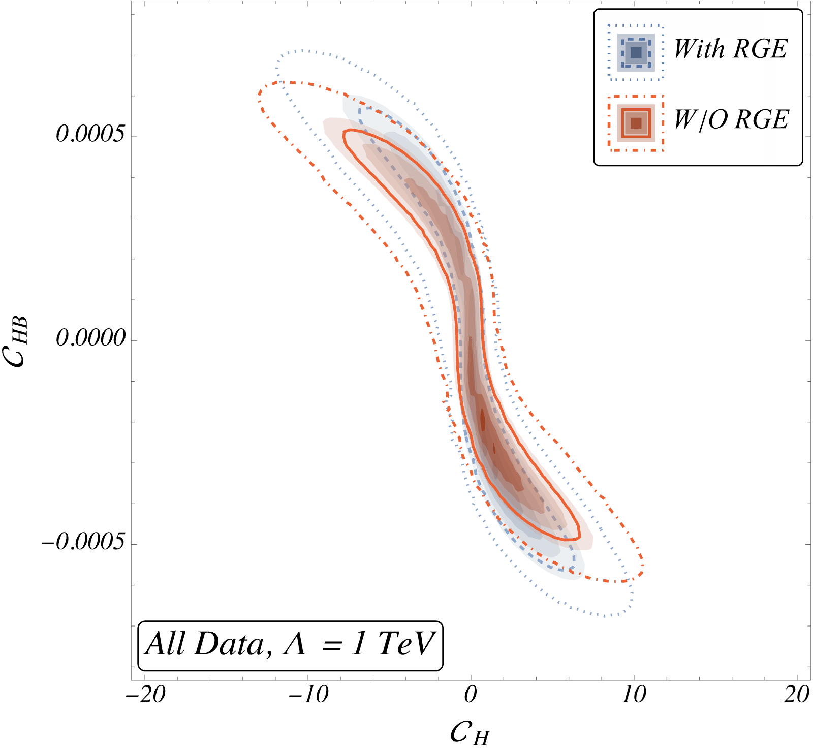
Refer to caption
(a) 𝒞Hsubscript𝒞𝐻\mathcal{C}_{H} - 𝒞HBsubscript𝒞𝐻𝐵\mathcal{C}_{HB}
Refer to caption
(b) 𝒞Hsubscript𝒞𝐻\mathcal{C}_{H\square} - 𝒞HDsubscript𝒞𝐻𝐷\mathcal{C}_{HD}
Refer to caption
(c) 𝒞HWsubscript𝒞𝐻𝑊\mathcal{C}_{HW} - 𝒞HWBsubscript𝒞𝐻𝑊𝐵\mathcal{C}_{HWB}
Refer to caption
(d) 𝒞Hsubscript𝒞𝐻\mathcal{C}_{H} - 𝒞HBsubscript𝒞𝐻𝐵\mathcal{C}_{HB}
Refer to caption
(e) 𝒞Hsubscript𝒞𝐻\mathcal{C}_{H\square} - 𝒞HDsubscript𝒞𝐻𝐷\mathcal{C}_{HD}
Refer to caption
(f) 𝒞HWsubscript𝒞𝐻𝑊\mathcal{C}_{HW} - 𝒞HWBsubscript𝒞𝐻𝑊𝐵\mathcal{C}_{HWB}
Figure 9: Two-dimensional posteriors among the WCs induced by 2subscript2\mathcal{H}_{2} for m2=subscript𝑚subscript2absentm_{\mathcal{H}_{2}}= 1 TeV (top row) and m2=3subscript𝑚subscript23m_{\mathcal{H}_{2}}=3 TeV (bottom row). Similar to fig. 8, the credible regions shown in red correspond to scenario without RGE and the blue ones with RGE.

After including the RG running of the SMEFT operators, the WC relations of 23 SMEFT operators are given as functions of the model parameters λ2,1,λ2,2subscript𝜆subscript21subscript𝜆subscript22\lambda_{\mathcal{H}_{2},1},\;\lambda_{\mathcal{H}_{2},2}, and λ2,3subscript𝜆subscript23\lambda_{\mathcal{H}_{2},3}. Thus, using the model parameter posterior distributions in the RG evolved matching relations, the multivariate distributions are obtained for these 23 WCs . This list includes some operators (for eg. QuBsubscript𝑄𝑢𝐵Q_{uB}, QuWsubscript𝑄𝑢𝑊Q_{uW}, QdBsubscript𝑄𝑑𝐵Q_{dB}, QdWsubscript𝑄𝑑𝑊Q_{dW}, QueBsubscript𝑄𝑢𝑒𝐵Q_{ueB}, QeWsubscript𝑄𝑒𝑊Q_{eW}) which are not constrained in the model-independent analysis by the experimental measurements. We show the example plots of such model-dependent WCs’ regions in fig. 10. The operators QuBsubscript𝑄𝑢𝐵Q_{uB}, QuWsubscript𝑄𝑢𝑊Q_{uW}, QeBsubscript𝑄𝑒𝐵Q_{eB} and QHudsubscript𝑄𝐻𝑢𝑑Q_{Hud} are RGE generated, and the corresponding WCs include an extra suppression of 1/16π2116superscript𝜋21/16\pi^{2}. The effect of this small factor is visible in the strictly constrained WC space.
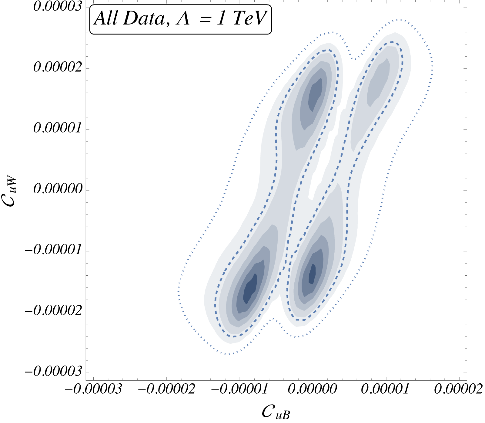
Refer to caption
(a) 𝒞uBsubscript𝒞𝑢𝐵\mathcal{C}_{uB} - 𝒞uWsubscript𝒞𝑢𝑊\mathcal{C}_{uW}
Refer to caption
(b) 𝒞eBsubscript𝒞𝑒𝐵\mathcal{C}_{eB} - 𝒞Hudsubscript𝒞𝐻𝑢𝑑\mathcal{C}_{Hud}
Figure 10: Two-dimensional marginalised WCs posterior for m2subscript𝑚subscript2m_{\mathcal{H}_{2}} (ΛΛ\Lambda) = 1 TeV with RG evolved matching results.

7 Conclusions

In this paper, we have analysed and constrained potential directions of beyond Standard Model physics under two themes: first, in a model-independent way using dimension-6 SMEFT and second for 161616 single scalar particle extensions of the SM using a similar statistical methodology and datasets.

We have performed a global analysis of 232323 Wilson coefficients in the Warsaw basis based on an up-to-date set of observables of the Higgs and di-boson sectors plus electroweak precision observables. Our fit includes di-Higgs measurements for the first time which improves the bounds on a modified Higgs potential through 𝒞Hsubscript𝒞𝐻\mathcal{C}_{H}. The addition of recent datasets, and in particular STXS data up to high energies, strengthens the limits on the Wilson coefficients by up to a factor 999 compared to previous analyses. The biggest improvements are obtained for operators describing Higgs-top and Higgs-gluon interactions as well as for 𝒞Hsubscript𝒞𝐻\mathcal{C}_{H\square}. We have analysed in detail the role of different STXS measurements in constraining the different Wilson coefficients.

Moreover, we have tabulated the complete sets of dimension-6 effective operators and the associated WCs in the Warsaw basis after integrating out the single heavy non-SM scalars for 161616 different new physics scenarios up to 1-loop level incorporating the scalar heavy-light mixing contributions from the loops. The WCs are expressed in terms of the model parameters. We have employed a similar analysis strategy for each of the BSM scenarios and constrained the model parameters. We have highlighted the individual impact of different observables (EWPO and Higgs data) through two-dimensional posteriors in model parameter as well as WC planes. We have explicitly discussed the results for the EWDS 2subscript2\mathcal{H}_{2} and a scalar leptoquark extension Θ1subscriptΘ1\Theta_{1}. Plots for the remaining 14 models considered are available in the Supplementary material SupMat 888These plots can also be downloaded from the GitHub repository Githubresult ..

We have investigated the effects of RG running on the allowed space of the model parameters and the WCs for two choices of the cut-off scale, 1 TeV and 3 TeV. We have performed the RG running (in leading-log approximation) on the matching results for an extra Electroweak scalar doublet model for two different cut-off scales 1 TeV and 3 TeV. We have noted that once the RG effects are taken into consideration, the allowed ranges of BSM parameters are relaxed compared to no RG case. We have also displayed the allowed ranges of WCs associated with the radiatively generated effective operators.

Currently, the considered dataset leaves some of the effective operators that arise from the single scalar extensions studied unconstrained and therefore fails to encapsulate the impact of all new physics interactions. Specifically, this concerns the WCs associated with 4-fermion operators. For the future, we are planning to add observables constraining 4-fermion operators Falkowski:2017pss , e.g. from dilepton production, parity violation and low-energy flavour observables, to constrain so far unbound directions in parameter space. These would be particularly relevant for constraining leptoquark models Schmaltz:2018nls .

8 Acknowledgement

We thank Julien Baglio, Silvia Ferrario Ravasio, Stephen Jones, Ken Mimasu, and Tevong You for helpful discussions, and Ennio Salvioni, Gauthier Durieux, and Matthew Mccullough for pointing out an error in matching result of the Quartet model (Σ)Σ(\Sigma). The work of A., S.D.B. and J.C. is supported by the Science and Engineering Research Board, Government of India, under the agreements SERB/PHY/2019501. SDB is also supported in part by SRA (Spain) under Grant No. PID2019-106087GB-C21 / 10.13039/501100011033; by the Junta de Andalucía (Spain) under Grants No. FQM- 101, A-FQM-467-UGR18, and P18-FR-4314 (FEDER). M.S. is supported by the STFC under grant ST/P001246/1. A.B. gratefully acknowledges support from the Alexander-von-Humboldt foundation as a Feodor Lynen Fellow. We thank the IPPP for access to its computing cluster.

Appendix A Functional matching by CoDEx

CoDEx uses effective action formulae to compute 1-loop level WCs, which involves solving functional “TraceLog𝑇𝑟𝑎𝑐𝑒𝐿𝑜𝑔Trace-Log” of UV action derivatives. We follow the procedures in Ref. Henning:2014wua (for loops with only heavy field propagators), and Refs. Zhang:2016pja and Ellis:2016enq for derivation and cross-checks of heavy-light mixed 1-loop effective action formulae, which CoDEx solves for each BSM. Note that there are more than one procedures to calculate the effective action formulae Henning:2014wua ; Drozd:2015rsp ; Fuentes-Martin:2016uol ; Zhang:2016pja . However, readers are welcome to study all of them as each method has its own advantages. It is worth mentioning that in this work we calculate matching of BSMs with single heavy scalar extension of the SM particle content, and therefore, the functional traces have a relatively simple form, which is not the case in most generic scenarios assuming arbitrary number of heavy fields with non-degenerate masses and arbitrary spins Fuentes-Martin:2020udw ; Cohen:2020qvb ; Kramer:2019fwz .

In the following text, we elaborate on the implementation of effective action formulae on BSMs to integrate out the heavy field up to 1-loop. The effective action Seff[ϕ]subscript𝑆effdelimited-[]italic-ϕS_{\text{eff}}[\phi] is defined

eiSeff[ϕ](μ)=𝒟ΦeiSUV[ϕ,Φ](μ),superscript𝑒𝑖subscript𝑆effdelimited-[]italic-ϕ𝜇𝒟Φsuperscript𝑒𝑖subscript𝑆UVitalic-ϕΦ𝜇\displaystyle e^{i\,S_{\text{eff}}[\phi](\mu)}=\int\mathcal{D}\Phi\,e^{i\,S_{\text{UV}}[\phi,\Phi](\mu)}, (13)

where, ΦΦ\Phi and ϕitalic-ϕ\phi represent are a heavy real scalar and a light field respectively, and SUV[ϕ,Φ](μ)subscript𝑆UVitalic-ϕΦ𝜇S_{\text{UV}}[\phi,\Phi](\mu) represents the UV action defines at scale μ𝜇\mu. In the following discussion, we set μ𝜇\mu equal to be the cut-off scale ΛΛ\Lambda, which is also the matching scale of the UV theory to the EFT. We expand the UV action around the classical configuration of the heavy field ΦcsubscriptΦ𝑐\Phi_{c} defined by,

δSUV[ϕ,Φ]δΦ|Φc=0.\displaystyle\left.\frac{\delta S_{\text{UV}}[\phi,\Phi]}{\delta\Phi}\right\rvert_{\Phi_{c}}=0. (14)

Now, SUV[ϕ,Φ]SUV[ϕ,Φc+η]subscript𝑆UVitalic-ϕΦsubscript𝑆UVitalic-ϕsubscriptΦ𝑐𝜂S_{\text{UV}}[\phi,\Phi]\rightarrow S_{\text{UV}}[\phi,\Phi_{c}+\eta] in Eq. 13, where η𝜂\eta represents the fluctuation field defined as Φ=Φc+ηΦsubscriptΦ𝑐𝜂\Phi=\Phi_{c}+\eta. Using Eq. 14, we have

Seff[ϕ]=SUV[ϕ,Φc]+i2TrLog[δ2SUV[ϕ,Φ]δΦ2|Φc]+𝒪(η2).\displaystyle S_{\text{eff}}[\phi]=S_{\text{UV}}[\phi,\Phi_{c}]+\frac{i}{2}\,\text{Tr}\,\text{Log}\left[\left.-\frac{\delta^{2}S_{\text{UV}}[\phi,\Phi]}{\delta\Phi^{2}}\right\rvert_{\Phi_{c}}\right]+\mathcal{O}(\eta^{2}). (15)

In Eq. 15, we recognize the first and second terms on the RHS as the tree-level and the pure heavy-loop processes in the effective action, respectively. Similarly, we can capture the contribution from the mixed heavy-light loop processes by expanding the UV action around the classical configuration of the light field(s), about which we discuss in detail at a later stage in this section. One can determine the classical configuration of the heavy field by using the Euler-Lagrange equation on the UV Lagrangian UVsubscriptUV\mathcal{L}_{\text{UV}}. Then substituting the heavy field solution back into the UV Lagrangian leads to tree-level matching. Subsequently, by imposing a mass-dimensions cut-off and Standard Model field Equation of Motions, Fierz identities, and Integration-by-Parts relations, one gets the Wilson coefficients of effective operators of a given mass dimension.

A.1 1-Loop matching: only heavy field as loop propagators

The functional “TraceLog𝑇𝑟𝑎𝑐𝑒𝐿𝑜𝑔Trace-Log” of action derivatives can be expanded in terms of covariant derivatives, quadratic matrix ‘U𝑈U’ and heavy field mass. The quadratic matrix ‘U𝑈U’ contains the interaction of heavy fields and light fields. We define

Seff1loop(H)(ϕ)superscriptsubscript𝑆eff1loop(H)italic-ϕ\displaystyle S_{\text{eff}}^{\text{1loop(H)}}(\phi) =i2Trlog[δ2SUV[ϕ,Φ]δΦ2|Φc]=icsTr log[P2+M2+U(ϕ)].\displaystyle=\frac{i}{2}\,\text{Tr}\,\text{log}\left[\left.-\frac{\delta^{2}S_{\text{UV}}[\phi,\Phi]}{\delta\Phi^{2}}\right\rvert_{\Phi_{c}}\right]=ic_{s}\text{Tr }\text{log}\left[-P^{2}+M^{2}+U(\phi)\right]. (16)

Here, M𝑀M is the mass of the heavy field ΦΦ\Phi. cssubscript𝑐𝑠c_{s} takes numerical values +1212+\frac{1}{2} and +11+1 for real and complex scalars respectively. Now, by expanding the functional trace by inserting a complete set of momentum and spatial states, and applying Baker-Campbell-Hausdorff formula Henning:2014wua , we get

Seff1loop(H)(ϕ)superscriptsubscript𝑆eff1loop(H)italic-ϕ\displaystyle S_{\text{eff}}^{\text{1loop(H)}}(\phi) =icsd4xd4k(2π)4trlog[(kμ+G~νμkν)2+M2+U~(ϕ)],absent𝑖subscript𝑐𝑠superscript𝑑4𝑥superscript𝑑4𝑘superscript2𝜋4trsuperscriptsubscript𝑘𝜇subscript~𝐺𝜈𝜇subscript𝑘𝜈2superscript𝑀2~𝑈italic-ϕ\displaystyle=ic_{s}\int d^{4}x\int\frac{d^{4}k}{(2\pi)^{4}}\text{tr}\,\log\left[-\left(k_{\mu}+\widetilde{G}_{\nu\mu}\frac{\partial}{\partial k_{\nu}}\right)^{2}+M^{2}+\widetilde{U}(\phi)\right], (17)

where,

G~νμ=n=0n+1(n+2)![Pα1,,[Pαn,[Pν,Pμ]]]nkα1kαn,subscript~𝐺𝜈𝜇superscriptsubscript𝑛0𝑛1𝑛2subscript𝑃subscript𝛼1subscript𝑃subscript𝛼𝑛subscript𝑃𝜈subscript𝑃𝜇superscript𝑛subscript𝑘subscript𝛼1subscript𝑘subscript𝛼𝑛\displaystyle\widetilde{G}_{\nu\mu}=-\sum_{n=0}^{\infty}\frac{n+1}{(n+2)!}\left[P_{\alpha_{1}},...,\left[P_{\alpha_{n}},\left[P_{\nu},P_{\mu}\right]\right]\right]\frac{\partial^{n}}{\partial k_{\alpha_{1}}...\partial k_{\alpha_{n}}}, (18)

and,

U~=n=01n![Pα1,,[Pαn,U]]nkα1kαn.~𝑈superscriptsubscript𝑛01𝑛subscript𝑃subscript𝛼1subscript𝑃subscript𝛼𝑛𝑈superscript𝑛subscript𝑘subscript𝛼1subscript𝑘subscript𝛼𝑛\displaystyle\widetilde{U}=\sum_{n=0}^{\infty}\frac{1}{n!}\left[P_{\alpha_{1}},...,\left[P_{\alpha_{n}},U\right]\right]\frac{\partial^{n}}{\partial k_{\alpha_{1}}...\partial k_{\alpha_{n}}}. (19)

This transformation puts all the covariant derivatives in commutators and hence, the resulting effective operators are manifestly gauge invariant. Now, we expand the argument of ‘log𝑙𝑜𝑔log’ and replace by an integral (on M2superscript𝑀2M^{2}),

Seff1loop(H)(ϕ)superscriptsubscript𝑆eff1loop(H)italic-ϕ\displaystyle S_{\text{eff}}^{\text{1loop(H)}}(\phi) =icsd4xd4k(2π)4𝑑M2tr[ΔF[1+ΔF({kμ,G~νμkν}+G~σμG~νσkμkνU~)]]1,absent𝑖subscript𝑐𝑠superscript𝑑4𝑥superscript𝑑4𝑘superscript2𝜋4differential-dsuperscript𝑀2trsuperscriptdelimited-[]subscriptΔ𝐹delimited-[]1subscriptΔ𝐹subscript𝑘𝜇subscript~𝐺𝜈𝜇subscript𝑘𝜈subscript~𝐺𝜎𝜇subscriptsuperscript~𝐺𝜎𝜈subscript𝑘𝜇subscript𝑘𝜈~𝑈1\displaystyle=-ic_{s}\int d^{4}x\int\frac{d^{4}k}{(2\pi)^{4}}\int dM^{2}\,\text{tr}\left[\Delta_{F}\left[1+\Delta_{F}\left(\left\{k_{\mu},\widetilde{G}_{\nu\mu}\frac{\partial}{\partial k_{\nu}}\right\}+\widetilde{G}_{\sigma\mu}\widetilde{G}^{\sigma}_{\nu}\frac{\partial}{\partial k_{\mu}}\frac{\partial}{\partial k_{\nu}}-\widetilde{U}\right)\right]\right]^{-1}, (20)

where, ΔF=1k2M2subscriptΔ𝐹1superscript𝑘2superscript𝑀2\Delta_{F}=\frac{1}{k^{2}-M^{2}}. The above equation is the master formula for gauge invariant effective operators up to arbitrary mass-dimension. In order to truncate at dimension-six, we expand the argument of ‘tr’ and replace the momentum integrals in terms of heavy field mass. Then, the effective action formula for pure-heavy-loop up to mass-dimension six is given by,

1loop(dim6)[ϕ]=subscriptsuperscript𝑑𝑖𝑚61𝑙𝑜𝑜𝑝delimited-[]italic-ϕabsent\displaystyle\mathcal{L}^{(dim-6)}_{1-loop}[\phi]= cs(4π)2tr{M2U+1M2[160(PμGμν)2190GμνGνσGσμ112(PμU)216U3112UGμνGμν]\displaystyle\frac{c_{s}}{(4\pi)^{2}}\,\text{tr}\,\Bigg{\{}M^{2}U+\frac{1}{M^{2}}\Bigg{[}-\frac{1}{60}\,\big{(}P_{\mu}G_{\mu\nu}^{\prime}\big{)}^{2}-\frac{1}{90}\,G_{\mu\nu}^{\prime}G_{\nu\sigma}^{\prime}G_{\sigma\mu}^{\prime}-\frac{1}{12}\,(P_{\mu}U)^{2}-\frac{1}{6}\,U^{3}-\frac{1}{12}\,UG_{\mu\nu}^{\prime}G_{\mu\nu}^{\prime}\Bigg{]}
+1M4[124U4+112U(PμU)2+1120(P2U)2+124(U2GμνGμν)1120[(PμU),(PνU)]Gμν\displaystyle+\frac{1}{M^{4}}\Bigg{[}\frac{1}{24}\,U^{4}+\frac{1}{12}\,U\big{(}P_{\mu}U\big{)}^{2}+\frac{1}{120}\,\big{(}P^{2}U\big{)}^{2}+\frac{1}{24}\,\Big{(}U^{2}G^{\prime}_{\mu\nu}G^{\prime}_{\mu\nu}\Big{)}-\frac{1}{120}\,\big{[}(P_{\mu}U),(P_{\nu}U)\big{]}G^{\prime}_{\mu\nu}
1120[U[U,Gμν]]Gμν]+1M6[160U5120U2(PμU)2130(UPμU)2]+1M8[1120U6]}.\displaystyle-\frac{1}{120}\,\big{[}U[U,G^{\prime}_{\mu\nu}]\big{]}G^{\prime}_{\mu\nu}\Bigg{]}+\frac{1}{M^{6}}\Bigg{[}-\frac{1}{60}\,U^{5}-\frac{1}{20}\,U^{2}\big{(}P_{\mu}U\big{)}^{2}-\frac{1}{30}\,\big{(}UP_{\mu}U\big{)}^{2}\Bigg{]}+\frac{1}{M^{8}}\bigg{[}\frac{1}{120}\,U^{6}\bigg{]}\Bigg{\}}\,. (21)

Here, Pμ=iDμandGμν=[Dμ,Dν]subscript𝑃𝜇𝑖subscript𝐷𝜇andsubscriptsuperscript𝐺𝜇𝜈subscript𝐷𝜇subscript𝐷𝜈P_{\mu}=i\ D_{\mu}\ \text{and}\ G^{\prime}_{\mu\nu}=[D_{\mu},D_{\nu}]. It is important to note down that ‘tr’ in the above equation is the trace performed over the internal symmetry indices. Note that the loop-level WCs are renomalization scheme dependent and are defined in MS¯¯MS\overline{\text{MS}} scheme.

CoDEx builds the covariant derivative operator for the heavy field from its SM quantum numbers, and constructs ‘U𝑈U’ from interactions present in the UV Lagrangian. Then, the field strength tensors in ‘Gμνsuperscriptsubscript𝐺𝜇𝜈G_{\mu\nu}^{\prime}’ are defined from the covariant derivative. For cases where, the heavy field transforms under both color and isospin groups, ‘U𝑈U’ would contain two pairs of indices, one each for SU(3)C𝑆𝑈subscript3𝐶SU(3)_{C} and SU(2)L𝑆𝑈subscript2𝐿SU(2)_{L} space of the field multiplet. Using all these information, the package evaluates the trace in Eq. A.1, and gets the effective Lagrangian in an off-shell basis, which is reduced to Warsaw (or other user-defined onshell) basis using onshell relations.

A.2 1-Loop matching: heavy-light loops

The mixed heavy-light contribution is derived by expanding the UV action around the classical configuration of light fields, similar to the pure heavy-loop approach. The 1-loop effective action ΔSeff1-loopΔsubscriptsuperscript𝑆1-loopeff\Delta S^{\text{1-loop}}_{\text{eff}} is defined as,

ΔSeff1-loop[ϕ,Φc]=i2Trlog[δ2SUV[ϕ,Φ]δ(ϕ,Φ)2|Φ=Φc(ϕ)].Δsubscriptsuperscript𝑆1-loopeffitalic-ϕsubscriptΦ𝑐𝑖2Trlogdelimited-[]evaluated-atsuperscript𝛿2subscript𝑆UVitalic-ϕΦ𝛿superscriptitalic-ϕΦ2ΦsubscriptΦ𝑐italic-ϕ\displaystyle\Delta S^{\text{1-loop}}_{\text{eff}}[\phi,\Phi_{c}]=\frac{i}{2}\text{Tr}\ \text{log}\left[\left.-\frac{\delta^{2}S_{\text{UV}}[\phi,\Phi]}{\delta(\phi,\Phi)^{2}}\right|_{\Phi=\Phi_{c}(\phi)}\right]. (22)

And we define,

QUV[ϕ,Φ]δ2SUV[ϕ,Φ]δ(ϕ,Φ)2.subscript𝑄UVitalic-ϕΦsuperscript𝛿2subscript𝑆UVitalic-ϕΦ𝛿superscriptitalic-ϕΦ2\displaystyle Q_{\text{UV}}[\phi,\Phi]\equiv-\frac{\delta^{2}S_{\text{UV}}[\phi,\Phi]}{\delta(\phi,\Phi)^{2}}. (23)

This contains quantum corrections from both heavy and light fields. Firstly, we block-diagonalize the quadratic matrix QUVsubscript𝑄UVQ_{\text{UV}}, which is a square matrix in the field space. We define ΔΔ\Delta’s following Eq. 23,

QUV[ϕ,Φ]=(ΔHΔHLΔLHΔL)(δ2SUV[ϕ,Φ]δΦ2δ2SUV[ϕ,Φ]δΦδϕδ2SUV[ϕ,Φ]δϕδΦδ2SUV[ϕ,Φ]δϕ2).subscript𝑄UVitalic-ϕΦmatrixsubscriptΔHsubscriptΔHLsubscriptΔLHsubscriptΔLmatrixsuperscript𝛿2subscript𝑆UVitalic-ϕΦ𝛿superscriptΦ2superscript𝛿2subscript𝑆UVitalic-ϕΦ𝛿Φ𝛿italic-ϕsuperscript𝛿2subscript𝑆UVitalic-ϕΦ𝛿italic-ϕ𝛿Φsuperscript𝛿2subscript𝑆UVitalic-ϕΦ𝛿superscriptitalic-ϕ2\displaystyle Q_{\text{UV}}[\phi,\Phi]=\begin{pmatrix}\Delta_{\text{H}}&\Delta_{\text{HL}}\\ \Delta_{\text{LH}}&\Delta_{\text{L}}\end{pmatrix}\equiv{\Large\begin{pmatrix}-\frac{\delta^{2}S_{\text{UV}}[\phi,\Phi]}{\delta\Phi^{2}}&-\frac{\delta^{2}S_{\text{UV}}[\phi,\Phi]}{\delta\Phi\delta\phi}\\ -\frac{\delta^{2}S_{\text{UV}}[\phi,\Phi]}{\delta\phi\delta\Phi}&-\frac{\delta^{2}S_{\text{UV}}[\phi,\Phi]}{\delta\phi^{2}}\end{pmatrix}}. (24)

Then, we define,

V=(𝟙𝟘ΔL1ΔLH𝟙)VQUVV=(ΔHΔHLΔL1ΔLH𝟘𝟘ΔL).\displaystyle V=\begin{pmatrix}\mathbb{1}&\mathbb{0}\\ -\Delta_{\text{L}}^{-1}\Delta_{\text{LH}}&\mathbb{1}\end{pmatrix}\hskip 30.00005pt\Rightarrow V^{\dagger}Q_{\text{UV}}V=\begin{pmatrix}\Delta_{\text{H}}-\Delta_{\text{HL}}\Delta_{\text{L}}^{-1}\Delta_{\text{LH}}&\mathbb{0}\\ \mathbb{0}&\Delta_{\text{L}}\end{pmatrix}. (25)

We use the distributive property of determinants,

ΔSeff1-loop[ϕ,Φc]Δsubscriptsuperscript𝑆1-loopeffitalic-ϕsubscriptΦ𝑐\displaystyle\Delta S^{\text{1-loop}}_{\text{eff}}[\phi,\Phi_{c}] =(i2Trlog[ΔHΔHLΔL1ΔLH]+i2Trlog[ΔL])|Φ=Φc.absentevaluated-at𝑖2Trlogdelimited-[]subscriptΔHsubscriptΔHLsuperscriptsubscriptΔL1subscriptΔLH𝑖2Trlogdelimited-[]subscriptΔLΦsubscriptΦ𝑐\displaystyle=\left.\left(\frac{i}{2}\text{Tr}\ \text{log}\left[\Delta_{\text{H}}-\Delta_{\text{HL}}\Delta_{\text{L}}^{-1}\Delta_{\text{LH}}\right]+\frac{i}{2}\text{Tr}\ \text{log}\left[\Delta_{\text{L}}\right]\right)\right|_{\Phi=\Phi_{c}}. (26)

Now, we define ΔΔ\Delta’s from the UV Lagrangian SUVsubscript𝑆UVS_{\text{UV}} in terms of the kinetic and interaction terms,

SUV[ϕ,Φ]subscript𝑆UVitalic-ϕΦ\displaystyle S_{\text{UV}}[\phi,\Phi] =d4xUV[ϕ,Φ]absentsuperscript𝑑4𝑥subscriptUVitalic-ϕΦ\displaystyle=\int d^{4}x\ \mathcal{L}_{\text{UV}}[\phi,\Phi]
ΔHabsentsubscriptΔH\displaystyle\Rightarrow-\Delta_{\text{H}} =δ2SUV[ϕ,Φ]δΦ2=d4xδ2UV[ϕ,Φ]δΦ2=d4x(𝒫2M2+UH),absentsuperscript𝛿2subscript𝑆UVitalic-ϕΦ𝛿superscriptΦ2superscript𝑑4𝑥superscript𝛿2subscriptUVitalic-ϕΦ𝛿superscriptΦ2superscript𝑑4𝑥superscript𝒫2superscript𝑀2subscript𝑈H\displaystyle=\frac{\delta^{2}S_{\text{UV}}[\phi,\Phi]}{\delta\Phi^{2}}=\int d^{4}x\ \frac{\delta^{2}\mathcal{L}_{\text{UV}}[\phi,\Phi]}{\delta\Phi^{2}}=\int d^{4}x\ \left(\mathcal{P}^{2}-M^{2}+U_{\text{H}}\right), (27)

where, 𝒫μi𝒟μsubscript𝒫𝜇𝑖subscript𝒟𝜇\mathcal{P}_{\mu}\equiv i\mathcal{D}_{\mu}, and, M2superscript𝑀2M^{2} is the squared mass matrix of ΦΦ\Phi. UHsubscript𝑈HU_{\text{H}} accommodates the light-field and self-interaction terms of ΦΦ\Phi in the UV Lagrangian. Similarly,

ΔLsubscriptΔL\displaystyle-\Delta_{\text{L}} =δ2SUV[ϕ,Φ]δϕ2=d4xδ2UV[ϕ,Φ]δϕ2=d4x(𝒫2m2+UL).absentsuperscript𝛿2subscript𝑆UVitalic-ϕΦ𝛿superscriptitalic-ϕ2superscript𝑑4𝑥superscript𝛿2subscriptUVitalic-ϕΦ𝛿superscriptitalic-ϕ2superscript𝑑4𝑥superscript𝒫2superscript𝑚2subscript𝑈L\displaystyle=\frac{\delta^{2}S_{\text{UV}}[\phi,\Phi]}{\delta\phi^{2}}=\int d^{4}x\ \frac{\delta^{2}\mathcal{L}_{\text{UV}}[\phi,\Phi]}{\delta\phi^{2}}=\int d^{4}x\ \left(\mathcal{P}^{2}-m^{2}+U_{\text{L}}\right). (28)

where, m𝑚m is the mass of ϕitalic-ϕ\phi. ULsubscript𝑈LU_{\text{L}} carries the heavy-field and self-interaction of the light field. The off-diagonal elements of QUVsubscript𝑄UVQ_{\text{UV}} are defined,

ΔHLsubscriptΔHL\displaystyle-\Delta_{\text{HL}} =δ2SUV[ϕ,Φ]δΦδϕ=d4xδ2UV[ϕ,Φ]δΦδϕ=d4xUHL,absentsuperscript𝛿2subscript𝑆UVitalic-ϕΦ𝛿Φ𝛿italic-ϕsuperscript𝑑4𝑥superscript𝛿2subscriptUVitalic-ϕΦ𝛿Φ𝛿italic-ϕsuperscript𝑑4𝑥subscript𝑈HL\displaystyle=\frac{\delta^{2}S_{\text{UV}}[\phi,\Phi]}{\delta\Phi\delta\phi}=\int d^{4}x\ \frac{\delta^{2}\mathcal{L}_{\text{UV}}[\phi,\Phi]}{\delta\Phi\delta\phi}=\int d^{4}x\ U_{\text{HL}}, (29)

and,

ΔLHsubscriptΔLH\displaystyle-\Delta_{\text{LH}} =δ2SUV[ϕ,Φ]δϕδΦ=d4xδ2UV[ϕ,Φ]δϕδΦ=d4xULH.absentsuperscript𝛿2subscript𝑆UVitalic-ϕΦ𝛿italic-ϕ𝛿Φsuperscript𝑑4𝑥superscript𝛿2subscriptUVitalic-ϕΦ𝛿italic-ϕ𝛿Φsuperscript𝑑4𝑥subscript𝑈LH\displaystyle=\frac{\delta^{2}S_{\text{UV}}[\phi,\Phi]}{\delta\phi\delta\Phi}=\int d^{4}x\ \frac{\delta^{2}\mathcal{L}_{\text{UV}}[\phi,\Phi]}{\delta\phi\delta\Phi}=\int d^{4}x\ U_{\text{LH}}. (30)

UHLsubscript𝑈HLU_{\text{HL}} and ULHsubscript𝑈LHU_{\text{LH}} carry the interactions between heavy ΦΦ\Phi and light ϕitalic-ϕ\phi fields. Now, we have defined R.H.S. of Eq. 26 completely in terms of interactions present in the Lagrangian. Then the next step is to extract the heavy-light mixed loop contribution from the R.H.S. We proceed by implementing the matching condition of a UV theory and its EFT:

ΓL,UV[ϕ]subscriptΓL,UVdelimited-[]italic-ϕ\displaystyle\Gamma_{\text{L,UV}}[\phi] =ΓEFT[ϕ],absentsubscriptΓEFTdelimited-[]italic-ϕ\displaystyle=\Gamma_{\text{EFT}}[\phi], (31)

where, ΓL,UV[ϕ]subscriptΓL,UVdelimited-[]italic-ϕ\Gamma_{\text{L,UV}}[\phi] is the 1-light-particle-irreducible(1LPI) effective action calculated in the UV theory, and ΓEFT[ϕ]subscriptΓEFTdelimited-[]italic-ϕ\Gamma_{\text{EFT}}[\phi] is the 1-particle-irreducible(1PI) effective action calculated in the EFT. This matching condition is imposed order by order in perturbation. At 1-loop order in UV,

ΓL,UV1-loop[ϕ]=ΔSeff1-loop[ϕ,Φc]=i2Trlog[QUV[ϕ,Φ]|Φ=Φc].superscriptsubscriptΓL,UV1-loopdelimited-[]italic-ϕΔsubscriptsuperscript𝑆1-loopeffitalic-ϕsubscriptΦ𝑐𝑖2Trlogdelimited-[]evaluated-atsubscript𝑄UVitalic-ϕΦΦsubscriptΦ𝑐\displaystyle\Gamma_{\text{L,UV}}^{\text{1-loop}}[\phi]=\Delta S^{\text{1-loop}}_{\text{eff}}[\phi,\Phi_{c}]=\frac{i}{2}\text{Tr}\ \text{log}\left[\left.Q_{\text{UV}}[\phi,\Phi]\right|_{\Phi=\Phi_{c}}\right]. (32)

Whereas at 1-loop order in EFT,

ΓEFT1-loop[ϕ]=d4xEFT1-loop[ϕ]+i2Trlog[δ2𝒮EFT[ϕ]δϕ2],subscriptsuperscriptΓ1-loopEFTdelimited-[]italic-ϕsuperscript𝑑4𝑥subscriptsuperscript1-loopEFTdelimited-[]italic-ϕ𝑖2Trlogdelimited-[]superscript𝛿2subscript𝒮EFTdelimited-[]italic-ϕ𝛿superscriptitalic-ϕ2\displaystyle\Gamma^{\text{1-loop}}_{\text{EFT}}[\phi]=\int d^{4}x\ \mathcal{L}^{\text{1-loop}}_{\text{EFT}}[\phi]+\frac{i}{2}\text{Tr}\ \text{log}\left[-\frac{\delta^{2}\mathcal{S_{\text{EFT}}}[\phi]}{\delta\phi^{2}}\right], (33)

where,

SEFT[ϕ]SUV[ϕ,Φc]=SUV[ϕ,Φ]|Φ=Φc(ϕ).subscript𝑆EFTdelimited-[]italic-ϕsubscript𝑆UVitalic-ϕsubscriptΦ𝑐evaluated-atsubscript𝑆UVitalic-ϕΦΦsubscriptΦ𝑐italic-ϕ\displaystyle S_{\text{EFT}}[\phi]\equiv S_{\text{UV}}[\phi,\Phi_{c}]=\left.S_{\text{UV}}[\phi,\Phi]\right|_{\Phi=\Phi_{c}(\phi)}. (34)

The 1-loop effective action in EFT contains contribution from (a) 1-loop generated operators contributing at tree-level, and (b) tree-level operators inserted at 1-loop. The R.H.S. of Eq. 33 contains these two contributions. Substituting Eqs. 32 and 33 in Eq. 31, we get

i2Trlog[QUV[ϕ,Φ]|Φ=Φc]=d4xEFT1-loop[ϕ]+i2Trlog[δ2𝒮EFT[ϕ]δϕ2]𝑖2Trlogdelimited-[]evaluated-atsubscript𝑄UVitalic-ϕΦΦsubscriptΦ𝑐superscript𝑑4𝑥subscriptsuperscript1-loopEFTdelimited-[]italic-ϕ𝑖2Trlogdelimited-[]superscript𝛿2subscript𝒮EFTdelimited-[]italic-ϕ𝛿superscriptitalic-ϕ2\displaystyle\frac{i}{2}\text{Tr}\ \text{log}\left[\left.Q_{\text{UV}}[\phi,\Phi]\right|_{\Phi=\Phi_{c}}\right]=\int d^{4}x\ \mathcal{L}^{\text{1-loop}}_{\text{EFT}}[\phi]+\frac{i}{2}\text{Tr}\ \text{log}\left[-\frac{\delta^{2}\mathcal{S_{\text{EFT}}}[\phi]}{\delta\phi^{2}}\right]
\displaystyle\implies d4xEFT1-loop[ϕ]=i2Trlog[QUV[ϕ,Φ]|Φ=Φc]i2Trlog[δ2𝒮EFT[ϕ]δϕ2].superscript𝑑4𝑥subscriptsuperscript1-loopEFTdelimited-[]italic-ϕ𝑖2Trlogdelimited-[]evaluated-atsubscript𝑄UVitalic-ϕΦΦsubscriptΦ𝑐𝑖2Trlogdelimited-[]superscript𝛿2subscript𝒮EFTdelimited-[]italic-ϕ𝛿superscriptitalic-ϕ2\displaystyle\int d^{4}x\ \mathcal{L}^{\text{1-loop}}_{\text{EFT}}[\phi]=\frac{i}{2}\text{Tr}\ \text{log}\left[\left.Q_{\text{UV}}[\phi,\Phi]\right|_{\Phi=\Phi_{c}}\right]-\frac{i}{2}\text{Tr}\ \text{log}\left[-\frac{\delta^{2}\mathcal{S_{\text{EFT}}}[\phi]}{\delta\phi^{2}}\right]. (35)

Now, we solve the second term in the R.H.S. of Eq. A.2,

δ2𝒮EFT[ϕ]δϕ2superscript𝛿2subscript𝒮EFTdelimited-[]italic-ϕ𝛿superscriptitalic-ϕ2\displaystyle-\frac{\delta^{2}\mathcal{S_{\text{EFT}}}[\phi]}{\delta\phi^{2}} =δ2δϕ2(SUV[ϕ,Φ]|Φ=Φc)=δδϕ{(δSUV[ϕ,Φ]δϕ+δΦδϕδSUV[ϕ,Φ]δΦ)|Φ=Φc}absentsuperscript𝛿2𝛿superscriptitalic-ϕ2evaluated-atsubscript𝑆UVitalic-ϕΦΦsubscriptΦ𝑐𝛿𝛿italic-ϕevaluated-at𝛿subscript𝑆UVitalic-ϕΦ𝛿italic-ϕ𝛿Φ𝛿italic-ϕ𝛿subscript𝑆UVitalic-ϕΦ𝛿ΦΦsubscriptΦ𝑐\displaystyle=-\frac{\delta^{2}}{\delta\phi^{2}}\left(\left.S_{\text{UV}}[\phi,\Phi]\right|_{\Phi=\Phi_{c}}\right)=-\frac{\delta}{\delta\phi}\left\{\left.\left(\frac{\delta S_{\text{UV}}[\phi,\Phi]}{\delta\phi}+\frac{\delta\Phi}{\delta\phi}\frac{\delta S_{\text{UV}}[\phi,\Phi]}{\delta\Phi}\right)\right|_{\Phi=\Phi_{c}}\right\}
=δδϕ(δSUV[ϕ,Φ]δϕ|Φ=Φc)=(δ2SUV[ϕ,Φ]δϕ2δΦδϕδ2SUV[ϕ,Φ]δΦδϕ)|Φ=Φcabsent𝛿𝛿italic-ϕevaluated-at𝛿subscript𝑆UVitalic-ϕΦ𝛿italic-ϕΦsubscriptΦ𝑐evaluated-atsuperscript𝛿2subscript𝑆UVitalic-ϕΦ𝛿superscriptitalic-ϕ2𝛿Φ𝛿italic-ϕsuperscript𝛿2subscript𝑆UVitalic-ϕΦ𝛿Φ𝛿italic-ϕΦsubscriptΦ𝑐\displaystyle=-\frac{\delta}{\delta\phi}\left(\left.\frac{\delta S_{\text{UV}}[\phi,\Phi]}{\delta\phi}\right|_{\Phi=\Phi_{c}}\right)=\left.\left(-\frac{\delta^{2}S_{\text{UV}}[\phi,\Phi]}{\delta\phi^{2}}-\frac{\delta\Phi}{\delta\phi}\frac{\delta^{2}S_{\text{UV}}[\phi,\Phi]}{\delta\Phi\delta\phi}\right)\right|_{\Phi=\Phi_{c}}
=(ΔLΔLHΔ^H1ΔHL)|Φ=Φc.absentevaluated-atsubscriptΔLsubscriptΔLHsuperscriptsubscript^ΔH1subscriptΔHLΦsubscriptΦ𝑐\displaystyle=\left.\left(\Delta_{\text{L}}-\Delta_{\text{LH}}\hat{\Delta}_{\text{H}}^{-1}\Delta_{\text{HL}}\right)\right|_{\Phi=\Phi_{c}}. (36)

We used the definition of ΦcsubscriptΦ𝑐\Phi_{c} on 1stsuperscript1st1^{\text{st}} line to come to 2ndsuperscript2nd2^{\text{nd}} line, and on 2ndsuperscript2nd2^{\text{nd}} line, we used

δδϕ(δSUV[ϕ,Φ]δΦ|Φ=Φc)=0𝛿𝛿italic-ϕevaluated-at𝛿subscript𝑆UVitalic-ϕΦ𝛿ΦΦsubscriptΦ𝑐0\displaystyle\frac{\delta}{\delta\phi}\left(\left.\frac{\delta S_{\text{UV}}[\phi,\Phi]}{\delta\Phi}\right|_{\Phi=\Phi_{c}}\right)=0
\displaystyle\implies (δ2SUV[ϕ,Φ]δϕδΦ+δΦδϕδ2SUV[ϕ,Φ]δΦ2)|Φ=Φc=0evaluated-atsuperscript𝛿2subscript𝑆UVitalic-ϕΦ𝛿italic-ϕ𝛿Φ𝛿Φ𝛿italic-ϕsuperscript𝛿2subscript𝑆UVitalic-ϕΦ𝛿superscriptΦ2ΦsubscriptΦ𝑐0\displaystyle\left.\left(\frac{\delta^{2}S_{\text{UV}}[\phi,\Phi]}{\delta\phi\delta\Phi}+\frac{\delta\Phi}{\delta\phi}\frac{\delta^{2}S_{\text{UV}}[\phi,\Phi]}{\delta\Phi^{2}}\right)\right|_{\Phi=\Phi_{c}}=0
\displaystyle\implies (δΦδϕΔH)|Φ=Φc=(ΔLH)|Φ=Φcevaluated-at𝛿Φ𝛿italic-ϕsubscriptΔHΦsubscriptΦ𝑐evaluated-atsubscriptΔLHΦsubscriptΦ𝑐\displaystyle\left.\left(\frac{\delta\Phi}{\delta\phi}\Delta_{\text{H}}\right)\right|_{\Phi=\Phi_{c}}=\left.\left(-\Delta_{\text{LH}}\right)\right|_{\Phi=\Phi_{c}}
\displaystyle\implies (δΦδϕ)|Φ=Φc=(ΔLH)|Φ=Φc(ΔH|Φ=Φc)1.evaluated-at𝛿Φ𝛿italic-ϕΦsubscriptΦ𝑐evaluated-atsubscriptΔLHΦsubscriptΦ𝑐superscriptevaluated-atsubscriptΔHΦsubscriptΦ𝑐1\displaystyle\left.\left(\frac{\delta\Phi}{\delta\phi}\right)\right|_{\Phi=\Phi_{c}}=\left.\left(-\Delta_{\text{LH}}\right)\right|_{\Phi=\Phi_{c}}\left(\left.\Delta_{\text{H}}\right|_{\Phi=\Phi_{c}}\right)^{-1}. (37)

to arrive at the 3rdsuperscript3rd3^{\text{rd}} line of Eq. A.2. The hat is put on ΔHsubscriptΔH\Delta_{\text{H}} to indicate that it is a local operator in the EFT. We rewrite Eq. A.2,

d4xEFT1-loop[ϕ]superscript𝑑4𝑥subscriptsuperscript1-loopEFTdelimited-[]italic-ϕ\displaystyle\int d^{4}x\ \mathcal{L}^{\text{1-loop}}_{\text{EFT}}[\phi]
=\displaystyle= (i2Trlog[ΔHΔHLΔL1ΔLH]+i2Trlog[ΔL]i2Trlog[ΔLΔLHΔ^H1ΔHL])|Φ=Φcevaluated-at𝑖2Trlogdelimited-[]subscriptΔHsubscriptΔHLsuperscriptsubscriptΔL1subscriptΔLH𝑖2Trlogdelimited-[]subscriptΔL𝑖2Trlogdelimited-[]subscriptΔLsubscriptΔLHsuperscriptsubscript^ΔH1subscriptΔHLΦsubscriptΦ𝑐\displaystyle\left.\left(\frac{i}{2}\text{Tr}\ \text{log}\left[\Delta_{\text{H}}-\Delta_{\text{HL}}\Delta_{\text{L}}^{-1}\Delta_{\text{LH}}\right]+\frac{i}{2}\text{Tr}\ \text{log}\left[\Delta_{\text{L}}\right]-\frac{i}{2}\text{Tr}\ \text{log}\left[\Delta_{\text{L}}-\Delta_{\text{LH}}\hat{\Delta}_{\text{H}}^{-1}\Delta_{\text{HL}}\right]\right)\right|_{\Phi=\Phi_{c}}
=\displaystyle= (i2Trlog[ΔHΔHLΔL1ΔLH]+i2Trlog[ΔL]\displaystyle\left.\left(\frac{i}{2}\text{Tr}\ \text{log}\left[\Delta_{\text{H}}-\Delta_{\text{HL}}\Delta_{\text{L}}^{-1}\Delta_{\text{LH}}\right]+\frac{i}{2}\text{Tr}\ \text{log}\left[\Delta_{\text{L}}\right]\right.\right.
i2Trlog[ΔL]i2Trlog[𝟙ΔL1ΔLHΔ^H1ΔHL])|Φ=Φc\displaystyle\left.\left.-\frac{i}{2}\text{Tr}\ \text{log}\left[\Delta_{\text{L}}\right]-\frac{i}{2}\text{Tr}\ \text{log}\left[\mathbb{1}-\Delta_{\text{L}}^{-1}\Delta_{\text{LH}}\hat{\Delta}_{\text{H}}^{-1}\Delta_{\text{HL}}\right]\right)\right|_{\Phi=\Phi_{c}}
=\displaystyle= (i2Trlog[ΔHΔHLΔL1ΔLH]i2Trlog[𝟙ΔL1ΔLHΔ^H1ΔHL])|Φ=Φc.evaluated-at𝑖2Trlogdelimited-[]subscriptΔHsubscriptΔHLsuperscriptsubscriptΔL1subscriptΔLH𝑖2Trlogdelimited-[]double-struck-𝟙superscriptsubscriptΔL1subscriptΔLHsuperscriptsubscript^ΔH1subscriptΔHLΦsubscriptΦ𝑐\displaystyle\left.\left(\frac{i}{2}\text{Tr}\ \text{log}\left[\Delta_{\text{H}}-\Delta_{\text{HL}}\Delta_{\text{L}}^{-1}\Delta_{\text{LH}}\right]-\frac{i}{2}\text{Tr}\ \text{log}\left[\mathbb{1}-\Delta_{\text{L}}^{-1}\Delta_{\text{LH}}\hat{\Delta}_{\text{H}}^{-1}\Delta_{\text{HL}}\right]\right)\right|_{\Phi=\Phi_{c}}. (38)

The contribution from loops with light propagators only (Trlog[ΔL]Trlogdelimited-[]subscriptΔL\text{Tr}\ \text{log}\ \left[\Delta_{\text{L}}\right]) , cancels while matching the UV theory to its EFT, as expected. We further reduce using Sylvester’s determinant identity on the second term,

(i2Trlog[ΔHΔHLΔL1ΔLH]i2Trlog[Δ^HΔHLΔL1ΔLH]+i2Trlog[Δ^H])|Φ=Φcevaluated-at𝑖2Trlogdelimited-[]subscriptΔHsubscriptΔHLsuperscriptsubscriptΔL1subscriptΔLH𝑖2Trlogdelimited-[]subscript^ΔHsubscriptΔHLsuperscriptsubscriptΔL1subscriptΔLH𝑖2Trlogdelimited-[]subscript^ΔHΦsubscriptΦ𝑐\displaystyle\left.\left(\frac{i}{2}\text{Tr}\ \text{log}\left[\Delta_{\text{H}}-\Delta_{\text{HL}}\Delta_{\text{L}}^{-1}\Delta_{\text{LH}}\right]-\frac{i}{2}\text{Tr}\ \text{log}\left[\hat{\Delta}_{\text{H}}-\Delta_{\text{HL}}\Delta_{\text{L}}^{-1}\Delta_{\text{LH}}\right]+\frac{i}{2}\text{Tr}\ \text{log}\left[\hat{\Delta}_{\text{H}}\right]\right)\right|_{\Phi=\Phi_{c}}
=\displaystyle= d4xEFT1-loop[ϕ].superscript𝑑4𝑥subscriptsuperscript1-loopEFTdelimited-[]italic-ϕ\displaystyle\int d^{4}x\ \mathcal{L}^{\text{1-loop}}_{\text{EFT}}[\phi]. (39)

Now, we have the contribution from both the heavy-light mixed loops and loops containing only heavy field propagators. One may cross-check the R.H.S. by substituting ΔL=ΔHL=ΔLH=0subscriptΔLsubscriptΔHLsubscriptΔLH0\Delta_{\text{L}}=\Delta_{\text{HL}}=\Delta_{\text{LH}}=0 and check that we get (i2Trlog[ΔH])|Φ=Φcevaluated-at𝑖2Trlogdelimited-[]subscriptΔHΦsubscriptΦ𝑐\left.\left(\frac{i}{2}\text{Tr}\ \text{log}\left[\Delta_{\text{H}}\right]\right)\right|_{\Phi=\Phi_{c}} , which contains loops with heavy field propagators only. The next step is to expand the R.H.S. of Eq. A.2 in terms of the covariant derivative operator, mass matrices and the quadratic matrix U’s, with a goal to construct an 1-loop effective action formula. We use the key observation made in Ref. Fuentes-Martin:2016uol , that the effective action can be split into “hard” and “soft” regions, and these regions produce the IR- and UV-divergent integrals, respectively. The hard region is captured when the loop integral is calculated in the limit M2m2much-greater-thansuperscript𝑀2superscript𝑚2M^{2}\gg m^{2}. So we solve,

d4xEFT1-loop[ϕ]=i2Trlog[ΔHΔHLΔL1ΔLH]|hardsuperscript𝑑4𝑥subscriptsuperscript1-loopEFTdelimited-[]italic-ϕevaluated-at𝑖2Trlogdelimited-[]subscriptΔHsubscriptΔHLsuperscriptsubscriptΔL1subscriptΔLHhard\displaystyle\int d^{4}x\ \mathcal{L}^{\text{1-loop}}_{\text{EFT}}[\phi]=\left.\frac{i}{2}\text{Tr}\ \text{log}\left[\Delta_{\text{H}}-\Delta_{\text{HL}}\Delta_{\text{L}}^{-1}\Delta_{\text{LH}}\right]\right|_{\text{hard}}
=\displaystyle= i2ddq(2π)dtrlog[ΔHΔHLΔL1ΔLH]|hardevaluated-at𝑖2superscript𝑑𝑑𝑞superscript2𝜋𝑑trlogdelimited-[]subscriptΔHsubscriptΔHLsuperscriptsubscriptΔL1subscriptΔLHhard\displaystyle\left.\frac{i}{2}\int\frac{d^{d}q}{(2\pi)^{d}}\,\text{tr}\ \text{log}\left[\Delta_{\text{H}}-\Delta_{\text{HL}}\Delta_{\text{L}}^{-1}\Delta_{\text{LH}}\right]\right|_{\text{hard}}
=\displaystyle= i2ddq(2π)dtrlog[(P22P.q+q2)+M2+UHΔHLΔL1ΔLH]|hard\displaystyle\left.\frac{i}{2}\int\frac{d^{d}q}{(2\pi)^{d}}\,\text{tr}\ \text{log}\left[-(P^{2}-2P.q+q^{2})+M^{2}+U_{\text{H}}-\Delta_{\text{HL}}\Delta_{\text{L}}^{-1}\Delta_{\text{LH}}\right]\right|_{\text{hard}}
=\displaystyle= i2n=11nddq(2π)dtrlog[(q2m2)1\displaystyle-\frac{i}{2}\sum_{n=1}^{\infty}\frac{1}{n}\int\frac{d^{d}q}{(2\pi)^{d}}\,\text{tr}\ \text{log}\left[(q^{2}-m^{2})^{-1}\right.
{P2+2P.q+UH|PPqΔHLΔL1ΔLH|PPq}]n|hard.\displaystyle\left.\left.\left\{-P^{2}+2P.q+\left.U_{\text{H}}\right|_{P\rightarrow P-q}-\left.\Delta_{\text{HL}}\Delta_{\text{L}}^{-1}\Delta_{\text{LH}}\right|_{P\rightarrow P-q}\right\}\right]^{n}\right|_{\text{hard}}. (40)

The last equality is true up to an additive constant because we factored out (q2M2)superscript𝑞2superscript𝑀2(q^{2}-M^{2}) and implemented the logarithmic expansion on the last step. Here, we expand the sum and keep terms encompassing all the dimension-6 (and lower) effective operators. To reduce these further, we follow the method of covariant diagrams as in Ref. Zhang:2016pja to arrive at the master formulae. The master trace formulae and their corresponding integration factors are tabulated in tabs. 5-8. These formulae are derived for single heavy field or multiple mass-degenerate heavy fields extension to the SM. We have compared these with that presented in Ref. Ellis:2017jns for mass-degenerate cases and we have found complete agreement.

Table 5: Effective action formulae with only U𝑈U’s. See tab. 9 for integration factor. The formula terms tabulated here, similar to the pure-heavy-loop effective action, are calculated using dimensional regularization and in MS¯¯𝑀𝑆\overline{MS} scheme. The matching scale is set equal to heavy field mass here.
Factors Formulae
ics11𝑖subscript𝑐𝑠superscript11-ic_{s}\mathcal{I}^{11} tr(UHLULH)subscript𝑈𝐻𝐿subscript𝑈𝐿𝐻\left(U_{HL}U_{LH}\right)
ics21𝑖subscript𝑐𝑠superscript21-ic_{s}\mathcal{I}^{21} tr(UHUHLULH)subscript𝑈𝐻subscript𝑈𝐻𝐿subscript𝑈𝐿𝐻\left(U_{H}U_{HL}U_{LH}\right)
ics31𝑖subscript𝑐𝑠superscript31-ic_{s}\mathcal{I}^{31} tr(UHUHUHLULH)subscript𝑈𝐻subscript𝑈𝐻subscript𝑈𝐻𝐿subscript𝑈𝐿𝐻\left(U_{H}U_{H}U_{HL}U_{LH}\right)
ics41𝑖subscript𝑐𝑠superscript41-ic_{s}\mathcal{I}^{41} tr(UHUHUHUHLULH)subscript𝑈𝐻subscript𝑈𝐻subscript𝑈𝐻subscript𝑈𝐻𝐿subscript𝑈𝐿𝐻\left(U_{H}U_{H}U_{H}U_{HL}U_{LH}\right)
ics51𝑖subscript𝑐𝑠superscript51-ic_{s}\mathcal{I}^{51} tr(UHUHUHUHUHLULH)subscript𝑈𝐻subscript𝑈𝐻subscript𝑈𝐻subscript𝑈𝐻subscript𝑈𝐻𝐿subscript𝑈𝐿𝐻\left(U_{H}U_{H}U_{H}U_{H}U_{HL}U_{LH}\right)
ics12𝑖subscript𝑐𝑠superscript12-ic_{s}\mathcal{I}^{12} tr(UHLULULH)subscript𝑈𝐻𝐿subscript𝑈𝐿subscript𝑈𝐿𝐻\left(U_{HL}U_{L}U_{LH}\right)
ics22𝑖subscript𝑐𝑠superscript22-ic_{s}\mathcal{I}^{22} tr(UHUHLULULH)subscript𝑈𝐻subscript𝑈𝐻𝐿subscript𝑈𝐿subscript𝑈𝐿𝐻\left(U_{H}U_{HL}U_{L}U_{LH}\right)
ics32𝑖subscript𝑐𝑠superscript32-ic_{s}\mathcal{I}^{32} tr(UHUHUHLULULH)subscript𝑈𝐻subscript𝑈𝐻subscript𝑈𝐻𝐿subscript𝑈𝐿subscript𝑈𝐿𝐻\left(U_{H}U_{H}U_{HL}U_{L}U_{LH}\right)
ics42𝑖subscript𝑐𝑠superscript42-ic_{s}\mathcal{I}^{42} tr(UHUHUHUHLULULH)subscript𝑈𝐻subscript𝑈𝐻subscript𝑈𝐻subscript𝑈𝐻𝐿subscript𝑈𝐿subscript𝑈𝐿𝐻\left(U_{H}U_{H}U_{H}U_{HL}U_{L}U_{LH}\right)
ics13𝑖subscript𝑐𝑠superscript13-ic_{s}\mathcal{I}^{13} tr(UHLULULULH)subscript𝑈𝐻𝐿subscript𝑈𝐿subscript𝑈𝐿subscript𝑈𝐿𝐻\left(U_{HL}U_{L}U_{L}U_{LH}\right)
ics23𝑖subscript𝑐𝑠superscript23-ic_{s}\mathcal{I}^{23} tr(UHUHLULULULH)subscript𝑈𝐻subscript𝑈𝐻𝐿subscript𝑈𝐿subscript𝑈𝐿subscript𝑈𝐿𝐻\left(U_{H}U_{HL}U_{L}U_{L}U_{LH}\right)
ics33𝑖subscript𝑐𝑠superscript33-ic_{s}\mathcal{I}^{33} tr(UHUHUHLULULULH)subscript𝑈𝐻subscript𝑈𝐻subscript𝑈𝐻𝐿subscript𝑈𝐿subscript𝑈𝐿subscript𝑈𝐿𝐻\left(U_{H}U_{H}U_{HL}U_{L}U_{L}U_{LH}\right)
ics14𝑖subscript𝑐𝑠superscript14-ic_{s}\mathcal{I}^{14} tr(UHLULULULULH)subscript𝑈𝐻𝐿subscript𝑈𝐿subscript𝑈𝐿subscript𝑈𝐿subscript𝑈𝐿𝐻\left(U_{HL}U_{L}U_{L}U_{L}U_{LH}\right)
(a)
Factors Formulae
ics24𝑖subscript𝑐𝑠superscript24-ic_{s}\mathcal{I}^{24} tr(UHUHLULULULULH)subscript𝑈𝐻subscript𝑈𝐻𝐿subscript𝑈𝐿subscript𝑈𝐿subscript𝑈𝐿subscript𝑈𝐿𝐻\left(U_{H}U_{HL}U_{L}U_{L}U_{L}U_{LH}\right)
ics15𝑖subscript𝑐𝑠superscript15-ic_{s}\mathcal{I}^{15} tr(UHLULULULULULH)subscript𝑈𝐻𝐿subscript𝑈𝐿subscript𝑈𝐿subscript𝑈𝐿subscript𝑈𝐿subscript𝑈𝐿𝐻\left(U_{HL}U_{L}U_{L}U_{L}U_{L}U_{LH}\right)
ics1222𝑖subscript𝑐𝑠12superscript22-ic_{s}\frac{1}{2}\mathcal{I}^{22} tr(UHLULHUHLULH)subscript𝑈𝐻𝐿subscript𝑈𝐿𝐻subscript𝑈𝐻𝐿subscript𝑈𝐿𝐻\left(U_{HL}U_{LH}U_{HL}U_{LH}\right)
ics32𝑖subscript𝑐𝑠superscript32-ic_{s}\mathcal{I}^{32} tr(UHUHLULHUHLULH)subscript𝑈𝐻subscript𝑈𝐻𝐿subscript𝑈𝐿𝐻subscript𝑈𝐻𝐿subscript𝑈𝐿𝐻\left(U_{H}U_{HL}U_{LH}U_{HL}U_{LH}\right)
ics1242𝑖subscript𝑐𝑠12superscript42-ic_{s}\frac{1}{2}\mathcal{I}^{42} tr(UHUHLULHUHUHLULH)subscript𝑈𝐻subscript𝑈𝐻𝐿subscript𝑈𝐿𝐻subscript𝑈𝐻subscript𝑈𝐻𝐿subscript𝑈𝐿𝐻\left(U_{H}U_{HL}U_{LH}U_{H}U_{HL}U_{LH}\right)
ics42𝑖subscript𝑐𝑠superscript42-ic_{s}\mathcal{I}^{42} tr(UHUHUHLULHUHLULH)subscript𝑈𝐻subscript𝑈𝐻subscript𝑈𝐻𝐿subscript𝑈𝐿𝐻subscript𝑈𝐻𝐿subscript𝑈𝐿𝐻\left(U_{H}U_{H}U_{HL}U_{LH}U_{HL}U_{LH}\right)
ics23𝑖subscript𝑐𝑠superscript23-ic_{s}\mathcal{I}^{23} tr(UHLULHUHLULULH)subscript𝑈𝐻𝐿subscript𝑈𝐿𝐻subscript𝑈𝐻𝐿subscript𝑈𝐿subscript𝑈𝐿𝐻\left(U_{HL}U_{LH}U_{HL}U_{L}U_{LH}\right)
ics33𝑖subscript𝑐𝑠superscript33-ic_{s}\mathcal{I}^{33} tr(UHUHLULHUHLULULH)subscript𝑈𝐻subscript𝑈𝐻𝐿subscript𝑈𝐿𝐻subscript𝑈𝐻𝐿subscript𝑈𝐿subscript𝑈𝐿𝐻\left(U_{H}U_{HL}U_{LH}U_{HL}U_{L}U_{LH}\right)
ics33𝑖subscript𝑐𝑠superscript33-ic_{s}\mathcal{I}^{33} tr(UHUHLULULHUHLULH)subscript𝑈𝐻subscript𝑈𝐻𝐿subscript𝑈𝐿subscript𝑈𝐿𝐻subscript𝑈𝐻𝐿subscript𝑈𝐿𝐻\left(U_{H}U_{HL}U_{L}U_{LH}U_{HL}U_{LH}\right)
ics1224𝑖subscript𝑐𝑠12superscript24-ic_{s}\frac{1}{2}\mathcal{I}^{24} tr(UHLULULHUHLULULH)subscript𝑈𝐻𝐿subscript𝑈𝐿subscript𝑈𝐿𝐻subscript𝑈𝐻𝐿subscript𝑈𝐿subscript𝑈𝐿𝐻\left(U_{HL}U_{L}U_{LH}U_{HL}U_{L}U_{LH}\right)
ics24𝑖subscript𝑐𝑠superscript24-ic_{s}\mathcal{I}^{24} tr(UHLULHUHLULULULH)subscript𝑈𝐻𝐿subscript𝑈𝐿𝐻subscript𝑈𝐻𝐿subscript𝑈𝐿subscript𝑈𝐿subscript𝑈𝐿𝐻\left(U_{HL}U_{LH}U_{HL}U_{L}U_{L}U_{LH}\right)
ics1333𝑖subscript𝑐𝑠13superscript33-ic_{s}\frac{1}{3}\mathcal{I}^{33} tr(UHLULHUHLULHUHLULH)subscript𝑈𝐻𝐿subscript𝑈𝐿𝐻subscript𝑈𝐻𝐿subscript𝑈𝐿𝐻subscript𝑈𝐻𝐿subscript𝑈𝐿𝐻\left(U_{HL}U_{LH}U_{HL}U_{LH}U_{HL}U_{LH}\right)
(b)
Table 6: Effective action formulae with two P𝑃P’s (Part-I).
Factors Formulae
fPU2=ics 2[q2]22subscriptsuperscript𝑓2𝑃𝑈𝑖subscript𝑐𝑠2superscriptdelimited-[]superscript𝑞222f^{{}^{2}}_{{}_{PU}}=-ic_{s}\ 2\,\mathcal{I}[q^{2}]^{22} tr([𝒫μ,UHL][𝒫μ,ULH])trsubscript𝒫𝜇subscript𝑈𝐻𝐿superscript𝒫𝜇subscript𝑈𝐿𝐻\text{tr}\left([\mathcal{P}_{\mu},U_{HL}][\mathcal{P}^{\mu},U_{LH}]\right)
fPU,a3(H)=ics 2([q2]32+[q2]41)subscriptsuperscript𝑓3𝐻𝑃𝑈𝑎𝑖subscript𝑐𝑠2superscriptdelimited-[]superscript𝑞232superscriptdelimited-[]superscript𝑞241f^{{}^{3(H)}}_{{}_{PU,a}}=-ic_{s}\,2\left(\mathcal{I}[q^{2}]^{32}+\mathcal{I}[q^{2}]^{41}\right) tr([𝒫μ,UH][𝒫μ,UHL]ULH)trsubscript𝒫𝜇subscript𝑈𝐻superscript𝒫𝜇subscript𝑈𝐻𝐿subscript𝑈𝐿𝐻\text{tr}\left([\mathcal{P}_{\mu},U_{H}][\mathcal{P}^{\mu},U_{HL}]U_{LH}\right)
fPU,b3(H)=ics 2([q2]32+[q2]41)subscriptsuperscript𝑓3𝐻𝑃𝑈𝑏𝑖subscript𝑐𝑠2superscriptdelimited-[]superscript𝑞232superscriptdelimited-[]superscript𝑞241f^{{}^{3(H)}}_{{}_{PU,b}}=-ic_{s}\,2\left(\mathcal{I}[q^{2}]^{32}+\mathcal{I}[q^{2}]^{41}\right) tr([𝒫μ,UH]UHL[𝒫μ,ULH])trsubscript𝒫𝜇subscript𝑈𝐻subscript𝑈𝐻𝐿superscript𝒫𝜇subscript𝑈𝐿𝐻\text{tr}\left([\mathcal{P}_{\mu},U_{H}]U_{HL}[\mathcal{P}^{\mu},U_{LH}]\right)
fPU,c3(H)=ics 4[q2]32subscriptsuperscript𝑓3𝐻𝑃𝑈𝑐𝑖subscript𝑐𝑠4superscriptdelimited-[]superscript𝑞232f^{{}^{3(H)}}_{{}_{PU,c}}=-ic_{s}\,4\,\mathcal{I}[q^{2}]^{32} tr(UH[𝒫μ,UHL][𝒫μ,ULH])trsubscript𝑈𝐻subscript𝒫𝜇subscript𝑈𝐻𝐿subscript𝒫𝜇subscript𝑈𝐿𝐻\text{tr}\left(U_{H}[\mathcal{P}_{\mu},U_{HL}][\mathcal{P}_{\mu},U_{LH}]\right)
fPU,a3(L)=ics 2([q2]14+[q2]23)subscriptsuperscript𝑓3𝐿𝑃𝑈𝑎𝑖subscript𝑐𝑠2superscriptdelimited-[]superscript𝑞214superscriptdelimited-[]superscript𝑞223f^{{}^{3(L)}}_{{}_{PU,a}}=-ic_{s}\,2\left(\mathcal{I}[q^{2}]^{14}+\mathcal{I}[q^{2}]^{23}\right) tr([𝒫μ,UHL][𝒫μ,UL]ULH)trsubscript𝒫𝜇subscript𝑈𝐻𝐿superscript𝒫𝜇subscript𝑈𝐿subscript𝑈𝐿𝐻\text{tr}\left([\mathcal{P}_{\mu},U_{HL}][\mathcal{P}^{\mu},U_{L}]U_{LH}\right)
fPU,b3(L)=ics 4[q2]23subscriptsuperscript𝑓3𝐿𝑃𝑈𝑏𝑖subscript𝑐𝑠4superscriptdelimited-[]superscript𝑞223f^{{}^{3(L)}}_{{}_{PU,b}}=-ic_{s}\,4\,\mathcal{I}[q^{2}]^{23} tr([𝒫μ,UHL]UL[𝒫μ,ULH])trsubscript𝒫𝜇subscript𝑈𝐻𝐿subscript𝑈𝐿superscript𝒫𝜇subscript𝑈𝐿𝐻\text{tr}\left([\mathcal{P}_{\mu},U_{HL}]U_{L}[\mathcal{P}^{\mu},U_{LH}]\right)
fPU,c3(L)=ics 2([q2]14+[q2]23)subscriptsuperscript𝑓3𝐿𝑃𝑈𝑐𝑖subscript𝑐𝑠2superscriptdelimited-[]superscript𝑞214superscriptdelimited-[]superscript𝑞223f^{{}^{3(L)}}_{{}_{PU,c}}=-ic_{s}\,2\left(\mathcal{I}[q^{2}]^{14}+\mathcal{I}[q^{2}]^{23}\right) tr(UHL[𝒫μ,UL][𝒫μ,ULH])trsubscript𝑈𝐻𝐿subscript𝒫𝜇subscript𝑈𝐿superscript𝒫𝜇subscript𝑈𝐿𝐻\text{tr}\left(U_{HL}[\mathcal{P}_{\mu},U_{L}][\mathcal{P}^{\mu},U_{LH}]\right)
Table 7: Effective action formulae with four P𝑃P’s.
Factors Formulae
fPPU,a2=ics 4([q4]33+2[q4]42+2[q4]51)subscriptsuperscript𝑓2𝑃𝑃𝑈𝑎𝑖subscript𝑐𝑠4superscriptdelimited-[]superscript𝑞4332superscriptdelimited-[]superscript𝑞4422superscriptdelimited-[]superscript𝑞451f^{{}^{2}}_{{}_{PPU,a}}=-ic_{s}\,4\left(\mathcal{I}[q^{4}]^{33}+2\mathcal{I}[q^{4}]^{42}+2\,\mathcal{I}[q^{4}]^{51}\right) tr(GμνGμνUHLULH)trsubscriptsuperscript𝐺𝜇𝜈superscript𝐺𝜇𝜈subscript𝑈𝐻𝐿subscript𝑈𝐿𝐻\text{tr}\left(G^{\prime}_{\mu\nu}G^{\prime\mu\nu}U_{HL}U_{LH}\right)
fPPU,b2=ics 4([q4]33+2[q4]24+2[q4]15)subscriptsuperscript𝑓2𝑃𝑃𝑈𝑏𝑖subscript𝑐𝑠4superscriptdelimited-[]superscript𝑞4332superscriptdelimited-[]superscript𝑞4242superscriptdelimited-[]superscript𝑞415f^{{}^{2}}_{{}_{PPU,b}}=-ic_{s}\,4\left(\mathcal{I}[q^{4}]^{33}+2\mathcal{I}[q^{4}]^{24}+2\,\mathcal{I}[q^{4}]^{15}\right) tr(GμνGμνULHUHL)trsubscriptsuperscript𝐺𝜇𝜈superscript𝐺𝜇𝜈subscript𝑈𝐿𝐻subscript𝑈𝐻𝐿\text{tr}\left(G^{\prime}_{\mu\nu}G^{\prime\mu\nu}U_{LH}U_{HL}\right)
fPPU,c2=ics 8[q4]33subscriptsuperscript𝑓2𝑃𝑃𝑈𝑐𝑖subscript𝑐𝑠8superscriptdelimited-[]superscript𝑞433f^{{}^{2}}_{{}_{PPU,c}}=-ic_{s}\,8\,\mathcal{I}[q^{4}]^{33} tr(Gνμ[𝒫μ,UHL][𝒫ν,ULH])trsubscriptsuperscript𝐺𝜈𝜇superscript𝒫𝜇subscript𝑈𝐻𝐿superscript𝒫𝜈subscript𝑈𝐿𝐻\text{tr}\left(G^{\prime}_{\nu\mu}[\mathcal{P}^{\mu},U_{HL}][\mathcal{P}^{\nu},U_{LH}]\right)
fPPU,d2=ics 8[q4]33subscriptsuperscript𝑓2𝑃𝑃𝑈𝑑𝑖subscript𝑐𝑠8superscriptdelimited-[]superscript𝑞433f^{{}^{2}}_{{}_{PPU,d}}=-ic_{s}\,8\,\mathcal{I}[q^{4}]^{33} tr(Gνμ[𝒫μ,ULH][𝒫ν,UHL])trsubscriptsuperscript𝐺𝜈𝜇superscript𝒫𝜇subscript𝑈𝐿𝐻superscript𝒫𝜈subscript𝑈𝐻𝐿\text{tr}\left(G^{\prime}_{\nu\mu}[\mathcal{P}^{\mu},U_{LH}][\mathcal{P}^{\nu},U_{HL}]\right)
fPPU,e2=ics 8[q4]33subscriptsuperscript𝑓2𝑃𝑃𝑈𝑒𝑖subscript𝑐𝑠8superscriptdelimited-[]superscript𝑞433f^{{}^{2}}_{{}_{PPU,e}}=-ic_{s}\,8\,\mathcal{I}[q^{4}]^{33} tr([𝒫μ,[𝒫μ,UHL]][𝒫ν,[𝒫ν,ULH]])trsubscript𝒫𝜇subscript𝒫𝜇subscript𝑈𝐻𝐿superscript𝒫𝜈superscript𝒫𝜈subscript𝑈𝐿𝐻\text{tr}\left(\left[\mathcal{P}_{\mu},\left[\mathcal{P}_{\mu},U_{HL}\right]\right]\left[\mathcal{P}^{\nu},\left[\mathcal{P}^{\nu},U_{LH}\right]\right]\right)
fPPU,f2=ics 4([q4]33+[q4]42)subscriptsuperscript𝑓2𝑃𝑃𝑈𝑓𝑖subscript𝑐𝑠4superscriptdelimited-[]superscript𝑞433superscriptdelimited-[]superscript𝑞442f^{{}^{2}}_{{}_{PPU,f}}=-ic_{s}\,4\,\left(\mathcal{I}[q^{4}]^{33}+\mathcal{I}[q^{4}]^{42}\right) tr([𝒫μ,UHL]ULH[𝒫ν,Gμν])trsuperscript𝒫𝜇subscript𝑈𝐻𝐿subscript𝑈𝐿𝐻superscript𝒫𝜈subscriptsuperscript𝐺𝜇𝜈\text{tr}\left([\mathcal{P}^{\mu},U_{HL}]U_{LH}[\mathcal{P}^{\nu},G^{\prime}_{\mu\nu}]\right)
fPPU,g2=ics 4([q4]33+[q4]42)subscriptsuperscript𝑓2𝑃𝑃𝑈𝑔𝑖subscript𝑐𝑠4superscriptdelimited-[]superscript𝑞433superscriptdelimited-[]superscript𝑞442f^{{}^{2}}_{{}_{PPU,g}}=-ic_{s}\,4\,\left(\mathcal{I}[q^{4}]^{33}+\mathcal{I}[q^{4}]^{42}\right) tr(UHL[𝒫μ,ULH][𝒫ν,Gνμ])trsubscript𝑈𝐻𝐿superscript𝒫𝜇subscript𝑈𝐿𝐻superscript𝒫𝜈subscriptsuperscript𝐺𝜈𝜇\text{tr}\left(U_{HL}\left[\mathcal{P}^{\mu},U_{LH}\right][\mathcal{P}^{\nu},G^{\prime}_{\nu\mu}]\right)
fPPU,h2=ics 4([q4]33+[q4]24)subscriptsuperscript𝑓2𝑃𝑃𝑈𝑖subscript𝑐𝑠4superscriptdelimited-[]superscript𝑞433superscriptdelimited-[]superscript𝑞424f^{{}^{2}}_{{}_{PPU,h}}=-ic_{s}\,4\,\left(\mathcal{I}[q^{4}]^{33}+\mathcal{I}[q^{4}]^{24}\right) tr(ULH[𝒫μ,UHL][𝒫ν,Gνμ])trsubscript𝑈𝐿𝐻superscript𝒫𝜇subscript𝑈𝐻𝐿superscript𝒫𝜈subscriptsuperscript𝐺𝜈𝜇\text{tr}\left(U_{LH}\left[\mathcal{P}^{\mu},U_{HL}\right][\mathcal{P}^{\nu},G^{\prime}_{\nu\mu}]\right)
fPPU,i2=ics 4([q4]33+[q4]24)subscriptsuperscript𝑓2𝑃𝑃𝑈𝑖𝑖subscript𝑐𝑠4superscriptdelimited-[]superscript𝑞433superscriptdelimited-[]superscript𝑞424f^{{}^{2}}_{{}_{PPU,i}}=-ic_{s}\,4\,\left(\mathcal{I}[q^{4}]^{33}+\mathcal{I}[q^{4}]^{24}\right) tr([𝒫μ,ULH]UHL[𝒫ν,Gμν])trsuperscript𝒫𝜇subscript𝑈𝐿𝐻subscript𝑈𝐻𝐿superscript𝒫𝜈subscriptsuperscript𝐺𝜇𝜈\text{tr}\left(\left[\mathcal{P}^{\mu},U_{LH}\right]U_{HL}[\mathcal{P}^{\nu},G^{\prime}_{\mu\nu}]\right)
Table 8: Effective action formulae with two P𝑃P’s (Part-II).
Factors Formulae
fPU,a4(HH)=ics 2([q2]42+2[q2]51)subscriptsuperscript𝑓4𝐻𝐻𝑃𝑈𝑎𝑖subscript𝑐𝑠2superscriptdelimited-[]superscript𝑞2422superscriptdelimited-[]superscript𝑞251f^{{}^{4(HH)}}_{{}_{PU,a}}=-ic_{s}\,2\,\left(\mathcal{I}[q^{2}]^{42}+2\,\mathcal{I}[q^{2}]^{51}\right) tr([𝒫μ,UH][𝒫μ,UH]UHLULH)trsubscript𝒫𝜇subscript𝑈𝐻superscript𝒫𝜇subscript𝑈𝐻subscript𝑈𝐻𝐿subscript𝑈𝐿𝐻\text{tr}\left([\mathcal{P}_{\mu},U_{H}][\mathcal{P}^{\mu},U_{H}]U_{HL}U_{LH}\right)
fPU,b4(HH)=ics 4([q2]42+[q2]51)subscriptsuperscript𝑓4𝐻𝐻𝑃𝑈𝑏𝑖subscript𝑐𝑠4superscriptdelimited-[]superscript𝑞242superscriptdelimited-[]superscript𝑞251f^{{}^{4(HH)}}_{{}_{PU,b}}=-ic_{s}\,4\,\left(\mathcal{I}[q^{2}]^{42}+\mathcal{I}[q^{2}]^{51}\right) tr([𝒫μ,UH]UH[𝒫μ,UHL]ULH)trsubscript𝒫𝜇subscript𝑈𝐻subscript𝑈𝐻superscript𝒫𝜇subscript𝑈𝐻𝐿subscript𝑈𝐿𝐻\text{tr}\left([\mathcal{P}_{\mu},U_{H}]U_{H}[\mathcal{P}^{\mu},U_{HL}]U_{LH}\right)
fPU,c4(HH)=ics 2([q2]42+2[q2]51)subscriptsuperscript𝑓4𝐻𝐻𝑃𝑈𝑐𝑖subscript𝑐𝑠2superscriptdelimited-[]superscript𝑞2422superscriptdelimited-[]superscript𝑞251f^{{}^{4(HH)}}_{{}_{PU,c}}=-ic_{s}\,2\,\left(\mathcal{I}[q^{2}]^{42}+2\,\mathcal{I}[q^{2}]^{51}\right) tr([𝒫μ,UH]UHUHL[𝒫μ,ULH])trsubscript𝒫𝜇subscript𝑈𝐻subscript𝑈𝐻subscript𝑈𝐻𝐿superscript𝒫𝜇subscript𝑈𝐿𝐻\text{tr}\left([\mathcal{P}_{\mu},U_{H}]U_{H}U_{HL}[\mathcal{P}^{\mu},U_{LH}]\right)
fPU,d4(HH)=ics 4([q2]42+[q2]51)subscriptsuperscript𝑓4𝐻𝐻𝑃𝑈𝑑𝑖subscript𝑐𝑠4superscriptdelimited-[]superscript𝑞242superscriptdelimited-[]superscript𝑞251f^{{}^{4(HH)}}_{{}_{PU,d}}=-ic_{s}\,4\,\left(\mathcal{I}[q^{2}]^{42}+\mathcal{I}[q^{2}]^{51}\right) tr(UH[𝒫μ,UH]UHL[𝒫μ,ULH])trsubscript𝑈𝐻subscript𝒫𝜇subscript𝑈𝐻subscript𝑈𝐻𝐿superscript𝒫𝜇subscript𝑈𝐿𝐻\text{tr}\left(U_{H}[\mathcal{P}_{\mu},U_{H}]U_{HL}[\mathcal{P}^{\mu},U_{LH}]\right)
fPU,e4(HH)=ics 6[q2]42subscriptsuperscript𝑓4𝐻𝐻𝑃𝑈𝑒𝑖subscript𝑐𝑠6superscriptdelimited-[]superscript𝑞242f^{{}^{4(HH)}}_{{}_{PU,e}}=-ic_{s}\,6\,\mathcal{I}[q^{2}]^{42} tr(UHUH[𝒫μ,UHL][𝒫μ,ULH])trsubscript𝑈𝐻subscript𝑈𝐻subscript𝒫𝜇subscript𝑈𝐻𝐿superscript𝒫𝜇subscript𝑈𝐿𝐻\text{tr}\left(U_{H}U_{H}[\mathcal{P}_{\mu},U_{HL}][\mathcal{P}^{\mu},U_{LH}]\right)
fPU,f4(HH)=ics 2([q2]42+2[q2]51)subscriptsuperscript𝑓4𝐻𝐻𝑃𝑈𝑓𝑖subscript𝑐𝑠2superscriptdelimited-[]superscript𝑞2422superscriptdelimited-[]superscript𝑞251f^{{}^{4(HH)}}_{{}_{PU,f}}=-ic_{s}\,2\,\left(\mathcal{I}[q^{2}]^{42}+2\,\mathcal{I}[q^{2}]^{51}\right) tr(UH[𝒫μ,UH][𝒫μ,UHL]ULH)trsubscript𝑈𝐻subscript𝒫𝜇subscript𝑈𝐻superscript𝒫𝜇subscript𝑈𝐻𝐿subscript𝑈𝐿𝐻\text{tr}\left(U_{H}[\mathcal{P}_{\mu},U_{H}][\mathcal{P}^{\mu},U_{HL}]U_{LH}\right)
fPU,a4(HL)=ics 2([q2]33+[q2]42)subscriptsuperscript𝑓4𝐻𝐿𝑃𝑈𝑎𝑖subscript𝑐𝑠2superscriptdelimited-[]superscript𝑞233superscriptdelimited-[]superscript𝑞242f^{{}^{4(HL)}}_{{}_{PU,a}}=-ic_{s}\,2\,\left(\mathcal{I}[q^{2}]^{33}+\,\mathcal{I}[q^{2}]^{42}\right) tr([𝒫μ,UH][𝒫μ,UHL]ULULH)trsubscript𝒫𝜇subscript𝑈𝐻superscript𝒫𝜇subscript𝑈𝐻𝐿subscript𝑈𝐿subscript𝑈𝐿𝐻\text{tr}\left([\mathcal{P}_{\mu},U_{H}][\mathcal{P}^{\mu},U_{HL}]U_{L}U_{LH}\right)
fPU,b4(HL)=ics 2([q2]33+2[q2]42)subscriptsuperscript𝑓4𝐻𝐿𝑃𝑈𝑏𝑖subscript𝑐𝑠2superscriptdelimited-[]superscript𝑞2332superscriptdelimited-[]superscript𝑞242f^{{}^{4(HL)}}_{{}_{PU,b}}=-ic_{s}\,2\,\left(\mathcal{I}[q^{2}]^{33}+2\,\mathcal{I}[q^{2}]^{42}\right) tr([𝒫μ,ULH][𝒫μ,UH]UHLUL)trsubscript𝒫𝜇subscript𝑈𝐿𝐻superscript𝒫𝜇subscript𝑈𝐻subscript𝑈𝐻𝐿subscript𝑈𝐿\text{tr}\left([\mathcal{P}_{\mu},U_{LH}][\mathcal{P}^{\mu},U_{H}]U_{HL}U_{L}\right)
fPU,c4(HL)=ics 2([q2]24+2[q2]33)subscriptsuperscript𝑓4𝐻𝐿𝑃𝑈𝑐𝑖subscript𝑐𝑠2superscriptdelimited-[]superscript𝑞2242superscriptdelimited-[]superscript𝑞233f^{{}^{4(HL)}}_{{}_{PU,c}}=-ic_{s}\,2\,\left(\mathcal{I}[q^{2}]^{24}+2\,\mathcal{I}[q^{2}]^{33}\right) tr(UHUHL[𝒫μ,UL][𝒫μ,ULH])trsubscript𝑈𝐻subscript𝑈𝐻𝐿subscript𝒫𝜇subscript𝑈𝐿superscript𝒫𝜇subscript𝑈𝐿𝐻\text{tr}\left(U_{H}U_{HL}[\mathcal{P}_{\mu},U_{L}][\mathcal{P}^{\mu},U_{LH}]\right)
fPU,d4(HL)=ics 2([q2]24+2[q2]33)subscriptsuperscript𝑓4𝐻𝐿𝑃𝑈𝑑𝑖subscript𝑐𝑠2superscriptdelimited-[]superscript𝑞2242superscriptdelimited-[]superscript𝑞233f^{{}^{4(HL)}}_{{}_{PU,d}}=-ic_{s}\,2\,\left(\mathcal{I}[q^{2}]^{24}+2\,\mathcal{I}[q^{2}]^{33}\right) tr(UH[𝒫μ,UHL][𝒫μ,UL]ULH)trsubscript𝑈𝐻subscript𝒫𝜇subscript𝑈𝐻𝐿superscript𝒫𝜇subscript𝑈𝐿subscript𝑈𝐿𝐻\text{tr}\left(U_{H}[\mathcal{P}_{\mu},U_{HL}][\mathcal{P}^{\mu},U_{L}]U_{LH}\right)
fPU,e4(HL)=ics 2([q2]24+2[q2]33+[q2]42)subscriptsuperscript𝑓4𝐻𝐿𝑃𝑈𝑒𝑖subscript𝑐𝑠2superscriptdelimited-[]superscript𝑞2242superscriptdelimited-[]superscript𝑞233superscriptdelimited-[]superscript𝑞242f^{{}^{4(HL)}}_{{}_{PU,e}}=-ic_{s}\,2\,\left(\mathcal{I}[q^{2}]^{24}+2\,\mathcal{I}[q^{2}]^{33}+\mathcal{I}[q^{2}]^{42}\right) tr([𝒫μ,UH]UHL[𝒫μ,UL]ULH)trsubscript𝒫𝜇subscript𝑈𝐻subscript𝑈𝐻𝐿superscript𝒫𝜇subscript𝑈𝐿subscript𝑈𝐿𝐻\text{tr}\left([\mathcal{P}_{\mu},U_{H}]U_{HL}[\mathcal{P}^{\mu},U_{L}]U_{LH}\right)
fPU,f4(HL)=ics 8([q2]33)subscriptsuperscript𝑓4𝐻𝐿𝑃𝑈𝑓𝑖subscript𝑐𝑠8superscriptdelimited-[]superscript𝑞233f^{{}^{4(HL)}}_{{}_{PU,f}}=-ic_{s}\,8\,\left(\mathcal{I}[q^{2}]^{33}\right) tr(UH[𝒫μ,UHL]UL[𝒫μ,ULH])trsubscript𝑈𝐻subscript𝒫𝜇subscript𝑈𝐻𝐿subscript𝑈𝐿superscript𝒫𝜇subscript𝑈𝐿𝐻\text{tr}\left(U_{H}[\mathcal{P}_{\mu},U_{HL}]U_{L}[\mathcal{P}^{\mu},U_{LH}]\right)
fPU,a4(LL)=ics 2(2[q2]15+[q2]24)subscriptsuperscript𝑓4𝐿𝐿𝑃𝑈𝑎𝑖subscript𝑐𝑠22superscriptdelimited-[]superscript𝑞215superscriptdelimited-[]superscript𝑞224f^{{}^{4(LL)}}_{{}_{PU,a}}=-ic_{s}\,2\left(2\mathcal{I}[q^{2}]^{15}+\mathcal{I}[q^{2}]^{24}\right) tr([𝒫μ,UHL][𝒫μ,UL]ULULH)trsubscript𝒫𝜇subscript𝑈𝐻𝐿superscript𝒫𝜇subscript𝑈𝐿subscript𝑈𝐿subscript𝑈𝐿𝐻\text{tr}\left([\mathcal{P}_{\mu},U_{HL}][\mathcal{P}^{\mu},U_{L}]U_{L}U_{LH}\right)
fPU,b4(LL)=ics 4([q2]15+[q2]24)subscriptsuperscript𝑓4𝐿𝐿𝑃𝑈𝑏𝑖subscript𝑐𝑠4superscriptdelimited-[]superscript𝑞215superscriptdelimited-[]superscript𝑞224f^{{}^{4(LL)}}_{{}_{PU,b}}=-ic_{s}\,4\left(\mathcal{I}[q^{2}]^{15}+\mathcal{I}[q^{2}]^{24}\right) tr([𝒫μ,UHL]UL[𝒫μ,UL]ULH)trsubscript𝒫𝜇subscript𝑈𝐻𝐿subscript𝑈𝐿superscript𝒫𝜇subscript𝑈𝐿subscript𝑈𝐿𝐻\text{tr}\left([\mathcal{P}_{\mu},U_{HL}]U_{L}[\mathcal{P}^{\mu},U_{L}]U_{LH}\right)
fPU,c4(LL)=ics 6[q2]24subscriptsuperscript𝑓4𝐿𝐿𝑃𝑈𝑐𝑖subscript𝑐𝑠6superscriptdelimited-[]superscript𝑞224f^{{}^{4(LL)}}_{{}_{PU,c}}=-ic_{s}\,6\mathcal{I}[q^{2}]^{24} tr([𝒫μ,UHL]ULUL[𝒫μ,ULH])trsubscript𝒫𝜇subscript𝑈𝐻𝐿subscript𝑈𝐿subscript𝑈𝐿superscript𝒫𝜇subscript𝑈𝐿𝐻\text{tr}\left([\mathcal{P}_{\mu},U_{HL}]U_{L}U_{L}[\mathcal{P}^{\mu},U_{LH}]\right)
fPU,d4(LL)=ics 2(2[q2]15+[q2]24)subscriptsuperscript𝑓4𝐿𝐿𝑃𝑈𝑑𝑖subscript𝑐𝑠22superscriptdelimited-[]superscript𝑞215superscriptdelimited-[]superscript𝑞224f^{{}^{4(LL)}}_{{}_{PU,d}}=-ic_{s}\,2\,\left(2\mathcal{I}[q^{2}]^{15}+\mathcal{I}[q^{2}]^{24}\right) tr(UHL[𝒫μ,UL][𝒫μ,UL]ULH)trsubscript𝑈𝐻𝐿subscript𝒫𝜇subscript𝑈𝐿superscript𝒫𝜇subscript𝑈𝐿subscript𝑈𝐿𝐻\text{tr}\left(U_{HL}[\mathcal{P}_{\mu},U_{L}][\mathcal{P}^{\mu},U_{L}]U_{LH}\right)
fPU,e4(LL)=ics 4([q2]15+[q2]24)subscriptsuperscript𝑓4𝐿𝐿𝑃𝑈𝑒𝑖subscript𝑐𝑠4superscriptdelimited-[]superscript𝑞215superscriptdelimited-[]superscript𝑞224f^{{}^{4(LL)}}_{{}_{PU,e}}=-ic_{s}\,4\left(\mathcal{I}[q^{2}]^{15}+\mathcal{I}[q^{2}]^{24}\right) tr(UHL[𝒫μ,UL]UL[𝒫μ,ULH])trsubscript𝑈𝐻𝐿subscript𝒫𝜇subscript𝑈𝐿subscript𝑈𝐿superscript𝒫𝜇subscript𝑈𝐿𝐻\text{tr}\left(U_{HL}[\mathcal{P}_{\mu},U_{L}]U_{L}[\mathcal{P}^{\mu},U_{LH}]\right)
fPU,f4(LL)=ics 2(2[q2]15+[q2]24)subscriptsuperscript𝑓4𝐿𝐿𝑃𝑈𝑓𝑖subscript𝑐𝑠22superscriptdelimited-[]superscript𝑞215superscriptdelimited-[]superscript𝑞224f^{{}^{4(LL)}}_{{}_{PU,f}}=-ic_{s}\,2\left(2\mathcal{I}[q^{2}]^{15}+\mathcal{I}[q^{2}]^{24}\right) tr(UHLUL[𝒫μ,UL][𝒫μ,ULH])trsubscript𝑈𝐻𝐿subscript𝑈𝐿subscript𝒫𝜇subscript𝑈𝐿superscript𝒫𝜇subscript𝑈𝐿𝐻\text{tr}\left(U_{HL}U_{L}[\mathcal{P}_{\mu},U_{L}][\mathcal{P}^{\mu},U_{LH}]\right)
fPU,a4(00)=ics([q2]24+2[q2]33+[q2]42)subscriptsuperscript𝑓400𝑃𝑈𝑎𝑖subscript𝑐𝑠superscriptdelimited-[]superscript𝑞2242superscriptdelimited-[]superscript𝑞233superscriptdelimited-[]superscript𝑞242f^{{}^{4(00)}}_{{}_{PU,a}}=-ic_{s}\,\left(\mathcal{I}[q^{2}]^{24}+2\,\mathcal{I}[q^{2}]^{33}+\mathcal{I}[q^{2}]^{42}\right) tr([𝒫μ,UHL]ULH[𝒫μ,UHL]ULH)trsubscript𝒫𝜇subscript𝑈𝐻𝐿subscript𝑈𝐿𝐻superscript𝒫𝜇subscript𝑈𝐻𝐿subscript𝑈𝐿𝐻\text{tr}\left([\mathcal{P}_{\mu},U_{HL}]U_{LH}[\mathcal{P}^{\mu},U_{HL}]U_{LH}\right)
fPU,b4(00)=ics 2([q2]24+2[q2]33)subscriptsuperscript𝑓400𝑃𝑈𝑏𝑖subscript𝑐𝑠2superscriptdelimited-[]superscript𝑞2242superscriptdelimited-[]superscript𝑞233f^{{}^{4(00)}}_{{}_{PU,b}}=-ic_{s}\,2\,\left(\mathcal{I}[q^{2}]^{24}+2\,\mathcal{I}[q^{2}]^{33}\right) tr([𝒫μ,UHL][𝒫μ,ULH]UHLULH)trsubscript𝒫𝜇subscript𝑈𝐻𝐿superscript𝒫𝜇subscript𝑈𝐿𝐻subscript𝑈𝐻𝐿subscript𝑈𝐿𝐻\text{tr}\left([\mathcal{P}_{\mu},U_{HL}][\mathcal{P}^{\mu},U_{LH}]U_{HL}U_{LH}\right)
fPU,c4(00)=ics 2(2[q2]33+[q2]42)subscriptsuperscript𝑓400𝑃𝑈𝑐𝑖subscript𝑐𝑠22superscriptdelimited-[]superscript𝑞233superscriptdelimited-[]superscript𝑞242f^{{}^{4(00)}}_{{}_{PU,c}}=-ic_{s}\,2\,\left(2\,\mathcal{I}[q^{2}]^{33}+\mathcal{I}[q^{2}]^{42}\right) tr([𝒫μ,UHL]ULHUHL[𝒫μ,ULH])trsubscript𝒫𝜇subscript𝑈𝐻𝐿subscript𝑈𝐿𝐻subscript𝑈𝐻𝐿superscript𝒫𝜇subscript𝑈𝐿𝐻\text{tr}\left([\mathcal{P}_{\mu},U_{HL}]U_{LH}U_{HL}[\mathcal{P}^{\mu},U_{LH}]\right)
fPU,d4(00)=ics([q2]24+2[q2]33+[q2]42)subscriptsuperscript𝑓400𝑃𝑈𝑑𝑖subscript𝑐𝑠superscriptdelimited-[]superscript𝑞2242superscriptdelimited-[]superscript𝑞233superscriptdelimited-[]superscript𝑞242f^{{}^{4(00)}}_{{}_{PU,d}}=-ic_{s}\,\left(\mathcal{I}[q^{2}]^{24}+2\,\mathcal{I}[q^{2}]^{33}+\mathcal{I}[q^{2}]^{42}\right) tr(UHL[𝒫μ,ULH]UHL[𝒫μ,ULH])trsubscript𝑈𝐻𝐿subscript𝒫𝜇subscript𝑈𝐿𝐻subscript𝑈𝐻𝐿superscript𝒫𝜇subscript𝑈𝐿𝐻\text{tr}\left(U_{HL}[\mathcal{P}_{\mu},U_{LH}]U_{HL}[\mathcal{P}^{\mu},U_{LH}]\right)
Table 9: Table of Integration factor (\mathcal{I}). Matching scale is equal to the heavy field mass μ=M𝜇𝑀\mu=M.
[q2n]αβ|n=0evaluated-atsuperscriptdelimited-[]superscript𝑞2𝑛𝛼𝛽𝑛0\left.\mathcal{I}\left[q^{2n}\right]^{\alpha\beta}\right|_{n=0} Factor ×i16π2absent𝑖16superscript𝜋2\times\frac{i}{16\pi^{2}} [q2n]αβ|n=1,2evaluated-atsuperscriptdelimited-[]superscript𝑞2𝑛𝛼𝛽𝑛12\left.\mathcal{I}\left[q^{2n}\right]^{\alpha\beta}\right|_{n=1,2} Factor ×i16π2absent𝑖16superscript𝜋2\times\frac{i}{16\pi^{2}}
11superscript11\mathcal{I}^{11} 111 [q2]13superscriptdelimited-[]superscript𝑞213\mathcal{I}\left[q^{2}\right]^{13} 38M238superscript𝑀2\frac{3}{8M^{2}}
12superscript12\mathcal{I}^{12} 1M21superscript𝑀2\frac{1}{M^{2}} [q2]22superscriptdelimited-[]superscript𝑞222\mathcal{I}\left[q^{2}\right]^{22} 14M214superscript𝑀2-\frac{1}{4M^{2}}
21superscript21\mathcal{I}^{21} 1M21superscript𝑀2-\frac{1}{M^{2}} [q2]31superscriptdelimited-[]superscript𝑞231\mathcal{I}\left[q^{2}\right]^{31} 18M218superscript𝑀2-\frac{1}{8M^{2}}
13superscript13\mathcal{I}^{13} 1M41superscript𝑀4\frac{1}{M^{4}} [q2]14superscriptdelimited-[]superscript𝑞214\mathcal{I}\left[q^{2}\right]^{14} 38M438superscript𝑀4\frac{3}{8M^{4}}
22superscript22\mathcal{I}^{22} 2M42superscript𝑀4-\frac{2}{M^{4}} [q2]23superscriptdelimited-[]superscript𝑞223\mathcal{I}\left[q^{2}\right]^{23} 58M458superscript𝑀4-\frac{5}{8M^{4}}
31superscript31\mathcal{I}^{31} 12M412superscript𝑀4\frac{1}{2M^{4}} [q2]32superscriptdelimited-[]superscript𝑞232\mathcal{I}\left[q^{2}\right]^{32} 18M418superscript𝑀4\frac{1}{8M^{4}}
14superscript14\mathcal{I}^{14} 1M61superscript𝑀6\frac{1}{M^{6}} [q2]41superscriptdelimited-[]superscript𝑞241\mathcal{I}\left[q^{2}\right]^{41} 124M4124superscript𝑀4\frac{1}{24M^{4}}
23superscript23\mathcal{I}^{23} 3M63superscript𝑀6-\frac{3}{M^{6}} [q2]15superscriptdelimited-[]superscript𝑞215\mathcal{I}\left[q^{2}\right]^{15} 38M638superscript𝑀6\frac{3}{8M^{6}}
32superscript32\mathcal{I}^{32} 52M652superscript𝑀6\frac{5}{2M^{6}} [q2]24superscriptdelimited-[]superscript𝑞224\mathcal{I}\left[q^{2}\right]^{24} 1M61superscript𝑀6-\frac{1}{M^{6}}
41superscript41\mathcal{I}^{41} 13M613superscript𝑀6-\frac{1}{3M^{6}} [q2]33superscriptdelimited-[]superscript𝑞233\mathcal{I}\left[q^{2}\right]^{33} 34M634superscript𝑀6\frac{3}{4M^{6}}
15superscript15\mathcal{I}^{15} 1M81superscript𝑀8\frac{1}{M^{8}} [q2]42superscriptdelimited-[]superscript𝑞242\mathcal{I}\left[q^{2}\right]^{42} 112M6112superscript𝑀6-\frac{1}{12M^{6}}
24superscript24\mathcal{I}^{24} 4M84superscript𝑀8-\frac{4}{M^{8}} [q2]51superscriptdelimited-[]superscript𝑞251\mathcal{I}\left[q^{2}\right]^{51} 148M6148superscript𝑀6-\frac{1}{48M^{6}}
33superscript33\mathcal{I}^{33} 112M8112superscript𝑀8\frac{11}{2M^{8}} [q2]51superscriptdelimited-[]superscript𝑞251\mathcal{I}\left[q^{2}\right]^{51} 148M6148superscript𝑀6-\frac{1}{48M^{6}}
42superscript42\mathcal{I}^{42} 176M8176superscript𝑀8-\frac{17}{6M^{8}} [q4]15superscriptdelimited-[]superscript𝑞415\mathcal{I}\left[q^{4}\right]^{15} 11144M411144superscript𝑀4\frac{11}{144M^{4}}
51superscript51\mathcal{I}^{51} 14M814superscript𝑀8\frac{1}{4M^{8}} [q4]24superscriptdelimited-[]superscript𝑞424\mathcal{I}\left[q^{4}\right]^{24} 17144M417144superscript𝑀4-\frac{17}{144M^{4}}
[q4]33superscriptdelimited-[]superscript𝑞433\mathcal{I}\left[q^{4}\right]^{33} 148M4148superscript𝑀4\frac{1}{48M^{4}}
[q4]42superscriptdelimited-[]superscript𝑞442\mathcal{I}\left[q^{4}\right]^{42} 1144M41144superscript𝑀4\frac{1}{144M^{4}}
[q4]42superscriptdelimited-[]superscript𝑞442\mathcal{I}\left[q^{4}\right]^{42} 1288M41288superscript𝑀4\frac{1}{288M^{4}}

Appendix B Matching results for scalar extended SM scenarios

B.1 Colour Singlet Heavy Scalars

Here, we have given the exhaustive sets of effective operators and the associated WCs that are emerged after integrating out the colour singlet heavy scalars up to 1-loop including the heavy-light mixing.

B.1.1 Real Singlet: 𝒮(1C,1L,0|Y\mathcal{S}\equiv(1_{C},1_{L},\left.0\right|_{Y})

Here, we have extended the SM by a real gauge singlet scalar (𝒮𝒮\mathcal{S}), and the modified Lagrangian involving this heavy field is written as Zhang:2016pja ; Jiang:2018pbd ; Dawson:2017vgm ; Haisch:2020ahr :

𝒮subscript𝒮\displaystyle\mathcal{L}_{\mathcal{S}} =SMd4+12(μ𝒮)212m𝒮2𝒮2c𝒮|H|2𝒮12κ𝒮|H|2𝒮213!μ𝒮𝒮314!λ𝒮𝒮4.absentsuperscriptsubscriptSM𝑑412superscriptsubscript𝜇𝒮212superscriptsubscript𝑚𝒮2superscript𝒮2subscript𝑐𝒮superscript𝐻2𝒮12subscript𝜅𝒮superscript𝐻2superscript𝒮213subscript𝜇𝒮superscript𝒮314subscript𝜆𝒮superscript𝒮4\displaystyle=\mathcal{L}_{{}_{\text{SM}}}^{d\leq 4}\;+\ \frac{1}{2}\ (\mathcal{\partial}_{\mu}\mathcal{S})^{2}\ -\ \frac{1}{2}\ m_{\mathcal{S}}^{2}\,\mathcal{S}^{2}-c_{\mathcal{S}}|H|^{2}\mathcal{S}-\frac{1}{2}\kappa_{\mathcal{S}}|H|^{2}\mathcal{S}^{2}-\frac{1}{3!}\,\mu_{\mathcal{S}}\,\mathcal{S}^{3}-\frac{1}{4!}\,\lambda_{\mathcal{S}}\,\mathcal{S}^{4}\,. (41)

Here, m𝒮subscript𝑚𝒮m_{\mathcal{S}} is mass of the heavy field (𝒮𝒮\mathcal{S}). This model contains four BSM parameters c𝒮,κ𝒮,μ𝒮,λ𝒮subscript𝑐𝒮subscript𝜅𝒮subscript𝜇𝒮subscript𝜆𝒮c_{\mathcal{S}},\kappa_{\mathcal{S}},\mu_{\mathcal{S}},\lambda_{\mathcal{S}}, and the WCs are functions of these parameters along with the SM ones, see tab. 10.

Table 10: Warsaw basis effective operators and the associated WCs that emerge after integrating-out the heavy field 𝒮:(1,1,0):𝒮110\mathcal{S}:(1,1,0). See caption of tab. 3 for colour coding.
Dim-6 Ops. Wilson coefficients
QdHsubscript𝑄dHQ_{\text{dH}} 3YdSMc𝒮2κ𝒮64π2m𝒮4+YdSMc𝒮3μ𝒮64π2m𝒮69YdSMc𝒮464π2m𝒮63superscriptsubscript𝑌𝑑SMsuperscriptsubscript𝑐𝒮2subscript𝜅𝒮64superscript𝜋2superscriptsubscript𝑚𝒮4superscriptsubscript𝑌𝑑SMsuperscriptsubscript𝑐𝒮3subscript𝜇𝒮64superscript𝜋2superscriptsubscript𝑚𝒮69superscriptsubscript𝑌𝑑SMsuperscriptsubscript𝑐𝒮464superscript𝜋2superscriptsubscript𝑚𝒮6-\frac{3Y_{d}^{\text{SM}}c_{\mathcal{S}}^{2}\kappa_{\mathcal{S}}}{64\pi^{2}m_{\mathcal{S}}^{4}}+\frac{Y_{d}^{\text{SM}}c_{\mathcal{S}}^{3}\mu_{\mathcal{S}}}{64\pi^{2}m_{\mathcal{S}}^{6}}-\frac{9Y_{d}^{\text{SM}}c_{\mathcal{S}}^{4}}{64\pi^{2}m_{\mathcal{S}}^{6}}
+29λHSMYdSMc𝒮2192π2m𝒮429superscriptsubscript𝜆𝐻SMsuperscriptsubscript𝑌𝑑SMsuperscriptsubscript𝑐𝒮2192superscript𝜋2superscriptsubscript𝑚𝒮4+\frac{29\lambda_{H}^{\text{SM}}Y_{d}^{\text{SM}}c_{\mathcal{S}}^{2}}{192\pi^{2}m_{\mathcal{S}}^{4}}
QeHsubscript𝑄eHQ_{\text{eH}} 3YeSMc𝒮2κ𝒮64π2m𝒮4+YeSMc𝒮3μ𝒮64π2m𝒮69YeSMc𝒮464π2m𝒮63superscriptsubscript𝑌𝑒SMsuperscriptsubscript𝑐𝒮2subscript𝜅𝒮64superscript𝜋2superscriptsubscript𝑚𝒮4superscriptsubscript𝑌𝑒SMsuperscriptsubscript𝑐𝒮3subscript𝜇𝒮64superscript𝜋2superscriptsubscript𝑚𝒮69superscriptsubscript𝑌𝑒SMsuperscriptsubscript𝑐𝒮464superscript𝜋2superscriptsubscript𝑚𝒮6-\frac{3Y_{e}^{\text{SM}}c_{\mathcal{S}}^{2}\kappa_{\mathcal{S}}}{64\pi^{2}m_{\mathcal{S}}^{4}}+\frac{Y_{e}^{\text{SM}}c_{\mathcal{S}}^{3}\mu_{\mathcal{S}}}{64\pi^{2}m_{\mathcal{S}}^{6}}-\frac{9Y_{e}^{\text{SM}}c_{\mathcal{S}}^{4}}{64\pi^{2}m_{\mathcal{S}}^{6}}
+29λHSMYeSMc𝒮2192π2m𝒮429superscriptsubscript𝜆𝐻SMsuperscriptsubscript𝑌𝑒SMsuperscriptsubscript𝑐𝒮2192superscript𝜋2superscriptsubscript𝑚𝒮4+\frac{29\lambda_{H}^{\text{SM}}Y_{e}^{\text{SM}}c_{\mathcal{S}}^{2}}{192\pi^{2}m_{\mathcal{S}}^{4}}
QuHsubscript𝑄uHQ_{\text{uH}} 3YuSMc𝒮2κ𝒮64π2m𝒮4+YuSMc𝒮3μ𝒮64π2m𝒮69YuSMc𝒮464π2m𝒮63superscriptsubscript𝑌𝑢SMsuperscriptsubscript𝑐𝒮2subscript𝜅𝒮64superscript𝜋2superscriptsubscript𝑚𝒮4superscriptsubscript𝑌𝑢SMsuperscriptsubscript𝑐𝒮3subscript𝜇𝒮64superscript𝜋2superscriptsubscript𝑚𝒮69superscriptsubscript𝑌𝑢SMsuperscriptsubscript𝑐𝒮464superscript𝜋2superscriptsubscript𝑚𝒮6-\frac{3Y_{u}^{\text{SM}}c_{\mathcal{S}}^{2}\kappa_{\mathcal{S}}}{64\pi^{2}m_{\mathcal{S}}^{4}}+\frac{Y_{u}^{\text{SM}}c_{\mathcal{S}}^{3}\mu_{\mathcal{S}}}{64\pi^{2}m_{\mathcal{S}}^{6}}-\frac{9Y_{u}^{\text{SM}}c_{\mathcal{S}}^{4}}{64\pi^{2}m_{\mathcal{S}}^{6}}
+29λHSMYuSMc𝒮2192π2m𝒮429superscriptsubscript𝜆𝐻SMsuperscriptsubscript𝑌𝑢SMsuperscriptsubscript𝑐𝒮2192superscript𝜋2superscriptsubscript𝑚𝒮4+\frac{29\lambda_{H}^{\text{SM}}Y_{u}^{\text{SM}}c_{\mathcal{S}}^{2}}{192\pi^{2}m_{\mathcal{S}}^{4}}
QHsubscript𝑄𝐻Q_{H} 43c𝒮648π2m𝒮87gW2λHSMc𝒮2288π2m𝒮4+41λHSMc𝒮2248π2m𝒮443superscriptsubscript𝑐𝒮648superscript𝜋2superscriptsubscript𝑚𝒮87superscriptsubscript𝑔𝑊2superscriptsubscript𝜆𝐻SMsuperscriptsubscript𝑐𝒮2288superscript𝜋2superscriptsubscript𝑚𝒮441superscriptsubscript𝜆𝐻SMsuperscriptsuperscriptsubscript𝑐𝒮2248superscript𝜋2superscriptsubscript𝑚𝒮4\frac{43c_{\mathcal{S}}^{6}}{48\pi^{2}m_{\mathcal{S}}^{8}}-\frac{7g_{W}^{2}\lambda_{H}^{\text{SM}}c_{\mathcal{S}}^{2}}{288\pi^{2}m_{\mathcal{S}}^{4}}+\frac{41\lambda_{H}^{\text{SM}}{}^{2}c_{\mathcal{S}}^{2}}{48\pi^{2}m_{\mathcal{S}}^{4}}
+37c𝒮4κ𝒮32π2m𝒮6+11c𝒮2κ𝒮232π2m𝒮4c𝒮2κ𝒮2m𝒮437superscriptsubscript𝑐𝒮4subscript𝜅𝒮32superscript𝜋2superscriptsubscript𝑚𝒮611superscriptsubscript𝑐𝒮2superscriptsubscript𝜅𝒮232superscript𝜋2superscriptsubscript𝑚𝒮4superscriptsubscript𝑐𝒮2subscript𝜅𝒮2superscriptsubscript𝑚𝒮4+\frac{37c_{\mathcal{S}}^{4}\kappa_{\mathcal{S}}}{32\pi^{2}m_{\mathcal{S}}^{6}}+\frac{11c_{\mathcal{S}}^{2}\kappa_{\mathcal{S}}^{2}}{32\pi^{2}m_{\mathcal{S}}^{4}}-\frac{c_{\mathcal{S}}^{2}\kappa_{\mathcal{S}}}{2m_{\mathcal{S}}^{4}}
c𝒮2κ𝒮λ𝒮32π2m𝒮4c𝒮4λ𝒮32π2m𝒮615c𝒮5μ𝒮32π2m𝒮8superscriptsubscript𝑐𝒮2subscript𝜅𝒮subscript𝜆𝒮32superscript𝜋2superscriptsubscript𝑚𝒮4superscriptsubscript𝑐𝒮4subscript𝜆𝒮32superscript𝜋2superscriptsubscript𝑚𝒮615superscriptsubscript𝑐𝒮5subscript𝜇𝒮32superscript𝜋2superscriptsubscript𝑚𝒮8-\frac{c_{\mathcal{S}}^{2}\kappa_{\mathcal{S}}\lambda_{\mathcal{S}}}{32\pi^{2}m_{\mathcal{S}}^{4}}-\frac{c_{\mathcal{S}}^{4}\lambda_{\mathcal{S}}}{32\pi^{2}m_{\mathcal{S}}^{6}}-\frac{15c_{\mathcal{S}}^{5}\mu_{\mathcal{S}}}{32\pi^{2}m_{\mathcal{S}}^{8}}
5c𝒮3κ𝒮μ𝒮16π2m𝒮6c𝒮κ𝒮2μ𝒮64π2m𝒮4+c𝒮3μ𝒮6m𝒮65superscriptsubscript𝑐𝒮3subscript𝜅𝒮subscript𝜇𝒮16superscript𝜋2superscriptsubscript𝑚𝒮6subscript𝑐𝒮superscriptsubscript𝜅𝒮2subscript𝜇𝒮64superscript𝜋2superscriptsubscript𝑚𝒮4superscriptsubscript𝑐𝒮3subscript𝜇𝒮6superscriptsubscript𝑚𝒮6-\frac{5c_{\mathcal{S}}^{3}\kappa_{\mathcal{S}}\mu_{\mathcal{S}}}{16\pi^{2}m_{\mathcal{S}}^{6}}-\frac{c_{\mathcal{S}}\kappa_{\mathcal{S}}^{2}\mu_{\mathcal{S}}}{64\pi^{2}m_{\mathcal{S}}^{4}}+\frac{c_{\mathcal{S}}^{3}\mu_{\mathcal{S}}}{6m_{\mathcal{S}}^{6}}
+c𝒮2κ𝒮μ𝒮232π2m𝒮6+c𝒮3λ𝒮μ𝒮48π2m𝒮6+c𝒮4μ𝒮216π2m𝒮8superscriptsubscript𝑐𝒮2subscript𝜅𝒮superscriptsubscript𝜇𝒮232superscript𝜋2superscriptsubscript𝑚𝒮6superscriptsubscript𝑐𝒮3subscript𝜆𝒮subscript𝜇𝒮48superscript𝜋2superscriptsubscript𝑚𝒮6superscriptsubscript𝑐𝒮4superscriptsubscript𝜇𝒮216superscript𝜋2superscriptsubscript𝑚𝒮8+\frac{c_{\mathcal{S}}^{2}\kappa_{\mathcal{S}}\mu_{\mathcal{S}}^{2}}{32\pi^{2}m_{\mathcal{S}}^{6}}+\frac{c_{\mathcal{S}}^{3}\lambda_{\mathcal{S}}\mu_{\mathcal{S}}}{48\pi^{2}m_{\mathcal{S}}^{6}}+\frac{c_{\mathcal{S}}^{4}\mu_{\mathcal{S}}^{2}}{16\pi^{2}m_{\mathcal{S}}^{8}}
57λHSMc𝒮432π2m𝒮6+13λHSMc𝒮3μ𝒮32π2m𝒮6c𝒮3μ𝒮396π2m𝒮857superscriptsubscript𝜆𝐻SMsuperscriptsubscript𝑐𝒮432superscript𝜋2superscriptsubscript𝑚𝒮613superscriptsubscript𝜆𝐻SMsuperscriptsubscript𝑐𝒮3subscript𝜇𝒮32superscript𝜋2superscriptsubscript𝑚𝒮6superscriptsubscript𝑐𝒮3superscriptsubscript𝜇𝒮396superscript𝜋2superscriptsubscript𝑚𝒮8-\frac{57\lambda_{H}^{\text{SM}}c_{\mathcal{S}}^{4}}{32\pi^{2}m_{\mathcal{S}}^{6}}+\frac{13\lambda_{H}^{\text{SM}}c_{\mathcal{S}}^{3}\mu_{\mathcal{S}}}{32\pi^{2}m_{\mathcal{S}}^{6}}-\frac{c_{\mathcal{S}}^{3}\mu_{\mathcal{S}}^{3}}{96\pi^{2}m_{\mathcal{S}}^{8}}
27λHSMc𝒮2κ𝒮32π2m𝒮4κ𝒮3192π2m𝒮227superscriptsubscript𝜆𝐻SMsuperscriptsubscript𝑐𝒮2subscript𝜅𝒮32superscript𝜋2superscriptsubscript𝑚𝒮4superscriptsubscript𝜅𝒮3192superscript𝜋2superscriptsubscript𝑚𝒮2-\frac{27\lambda_{H}^{\text{SM}}c_{\mathcal{S}}^{2}\kappa_{\mathcal{S}}}{32\pi^{2}m_{\mathcal{S}}^{4}}-\frac{\kappa_{\mathcal{S}}^{3}}{192\pi^{2}m_{\mathcal{S}}^{2}}
QHsubscript𝑄𝐻Q_{H\square} 13c𝒮4192π2m𝒮6c𝒮22m𝒮47gW2c𝒮2384π2m𝒮413superscriptsubscript𝑐𝒮4192superscript𝜋2superscriptsubscript𝑚𝒮6superscriptsubscript𝑐𝒮22superscriptsubscript𝑚𝒮47superscriptsubscript𝑔𝑊2superscriptsubscript𝑐𝒮2384superscript𝜋2superscriptsubscript𝑚𝒮4\frac{13c_{\mathcal{S}}^{4}}{192\pi^{2}m_{\mathcal{S}}^{6}}-\frac{c_{\mathcal{S}}^{2}}{2m_{\mathcal{S}}^{4}}-\frac{7g_{W}^{2}c_{\mathcal{S}}^{2}}{384\pi^{2}m_{\mathcal{S}}^{4}}
+25c𝒮2κ𝒮192π2m𝒮4c𝒮2λ𝒮32π2m𝒮413c𝒮3μ𝒮192π2m𝒮625superscriptsubscript𝑐𝒮2subscript𝜅𝒮192superscript𝜋2superscriptsubscript𝑚𝒮4superscriptsubscript𝑐𝒮2subscript𝜆𝒮32superscript𝜋2superscriptsubscript𝑚𝒮413superscriptsubscript𝑐𝒮3subscript𝜇𝒮192superscript𝜋2superscriptsubscript𝑚𝒮6+\frac{25c_{\mathcal{S}}^{2}\kappa_{\mathcal{S}}}{192\pi^{2}m_{\mathcal{S}}^{4}}-\frac{c_{\mathcal{S}}^{2}\lambda_{\mathcal{S}}}{32\pi^{2}m_{\mathcal{S}}^{4}}-\frac{13c_{\mathcal{S}}^{3}\mu_{\mathcal{S}}}{192\pi^{2}m_{\mathcal{S}}^{6}}
κ𝒮2384π2m𝒮2+11c𝒮2μ𝒮2384π2m𝒮65c𝒮κ𝒮μ𝒮192π2m𝒮4superscriptsubscript𝜅𝒮2384superscript𝜋2superscriptsubscript𝑚𝒮211superscriptsubscript𝑐𝒮2superscriptsubscript𝜇𝒮2384superscript𝜋2superscriptsubscript𝑚𝒮65subscript𝑐𝒮subscript𝜅𝒮subscript𝜇𝒮192superscript𝜋2superscriptsubscript𝑚𝒮4-\frac{\kappa_{\mathcal{S}}^{2}}{384\pi^{2}m_{\mathcal{S}}^{2}}+\frac{11c_{\mathcal{S}}^{2}\mu_{\mathcal{S}}^{2}}{384\pi^{2}m_{\mathcal{S}}^{6}}-\frac{5c_{\mathcal{S}}\kappa_{\mathcal{S}}\mu_{\mathcal{S}}}{192\pi^{2}m_{\mathcal{S}}^{4}}
7gY2c𝒮21152π2m𝒮47superscriptsubscript𝑔𝑌2superscriptsubscript𝑐𝒮21152superscript𝜋2superscriptsubscript𝑚𝒮4-\frac{7g_{Y}^{2}c_{\mathcal{S}}^{2}}{1152\pi^{2}m_{\mathcal{S}}^{4}}
(a)
Dim-6 Ops. Wilson coefficients
QHBsubscript𝑄HBQ_{\text{HB}} gY2c𝒮2256π2m𝒮4superscriptsubscript𝑔𝑌2superscriptsubscript𝑐𝒮2256superscript𝜋2superscriptsubscript𝑚𝒮4\frac{g_{Y}^{2}c_{\mathcal{S}}^{2}}{256\pi^{2}m_{\mathcal{S}}^{4}}
QHDsubscript𝑄HDQ_{\text{HD}} 7gY2c𝒮2288π2m𝒮47superscriptsubscript𝑔𝑌2superscriptsubscript𝑐𝒮2288superscript𝜋2superscriptsubscript𝑚𝒮4-\frac{7g_{Y}^{2}c_{\mathcal{S}}^{2}}{288\pi^{2}m_{\mathcal{S}}^{4}}
QHdsubscript𝑄HdQ_{\text{Hd}} 7gY2c𝒮21728π2m𝒮47superscriptsubscript𝑔𝑌2superscriptsubscript𝑐𝒮21728superscript𝜋2superscriptsubscript𝑚𝒮4\frac{7g_{Y}^{2}c_{\mathcal{S}}^{2}}{1728\pi^{2}m_{\mathcal{S}}^{4}}
QHesubscript𝑄HeQ_{\text{He}} 7gY2c𝒮2576π2m𝒮47superscriptsubscript𝑔𝑌2superscriptsubscript𝑐𝒮2576superscript𝜋2superscriptsubscript𝑚𝒮4\frac{7g_{Y}^{2}c_{\mathcal{S}}^{2}}{576\pi^{2}m_{\mathcal{S}}^{4}}
QHusubscript𝑄HuQ_{\text{Hu}} 7gY2c𝒮2864π2m𝒮47superscriptsubscript𝑔𝑌2superscriptsubscript𝑐𝒮2864superscript𝜋2superscriptsubscript𝑚𝒮4-\frac{7g_{Y}^{2}c_{\mathcal{S}}^{2}}{864\pi^{2}m_{\mathcal{S}}^{4}}
QHWsubscript𝑄HWQ_{\text{HW}} gW2c𝒮2256π2m𝒮4superscriptsubscript𝑔𝑊2superscriptsubscript𝑐𝒮2256superscript𝜋2superscriptsubscript𝑚𝒮4\frac{g_{W}^{2}c_{\mathcal{S}}^{2}}{256\pi^{2}m_{\mathcal{S}}^{4}}
QHWBsubscript𝑄HWBQ_{\text{HWB}} gWgYc𝒮2128π2m𝒮4subscript𝑔𝑊subscript𝑔𝑌superscriptsubscript𝑐𝒮2128superscript𝜋2superscriptsubscript𝑚𝒮4\frac{g_{W}g_{Y}c_{\mathcal{S}}^{2}}{128\pi^{2}m_{\mathcal{S}}^{4}}
QHl(1)Q_{\text{Hl}}{}^{(1)} 7gY2c𝒮21152π2m𝒮47superscriptsubscript𝑔𝑌2superscriptsubscript𝑐𝒮21152superscript𝜋2superscriptsubscript𝑚𝒮4\frac{7g_{Y}^{2}c_{\mathcal{S}}^{2}}{1152\pi^{2}m_{\mathcal{S}}^{4}}
QHq(1)Q_{\text{Hq}}{}^{(1)} 7gY2c𝒮23456π2m𝒮47superscriptsubscript𝑔𝑌2superscriptsubscript𝑐𝒮23456superscript𝜋2superscriptsubscript𝑚𝒮4-\frac{7g_{Y}^{2}c_{\mathcal{S}}^{2}}{3456\pi^{2}m_{\mathcal{S}}^{4}}
QHl(3)Q_{\text{Hl}}{}^{(3)} 7gW2c𝒮21152π2m𝒮47superscriptsubscript𝑔𝑊2superscriptsubscript𝑐𝒮21152superscript𝜋2superscriptsubscript𝑚𝒮4-\frac{7g_{W}^{2}c_{\mathcal{S}}^{2}}{1152\pi^{2}m_{\mathcal{S}}^{4}}
QHq(3)Q_{\text{Hq}}{}^{(3)} 7gW2c𝒮21152π2m𝒮47superscriptsubscript𝑔𝑊2superscriptsubscript𝑐𝒮21152superscript𝜋2superscriptsubscript𝑚𝒮4-\frac{7g_{W}^{2}c_{\mathcal{S}}^{2}}{1152\pi^{2}m_{\mathcal{S}}^{4}}
Qlequ(1)Q_{\text{lequ}}{}^{(1)} YeSMYuSMc𝒮296π2m𝒮4superscriptsubscript𝑌𝑒SMsuperscriptsubscript𝑌𝑢SMsuperscriptsubscript𝑐𝒮296superscript𝜋2superscriptsubscript𝑚𝒮4\frac{Y_{e}^{\text{SM}}Y_{u}^{\text{SM}}c_{\mathcal{S}}^{2}}{96\pi^{2}m_{\mathcal{S}}^{4}}
Qqd(1)Q_{\text{qd}}{}^{(1)} YdSMYdSMc𝒮2192π2m𝒮4superscriptsubscript𝑌𝑑SMsuperscriptsubscript𝑌𝑑SMsuperscriptsubscript𝑐𝒮2192superscript𝜋2superscriptsubscript𝑚𝒮4-\frac{Y_{d}^{\text{SM}}Y_{d}^{\text{SM$\dagger$}}c_{\mathcal{S}}^{2}}{192\pi^{2}m_{\mathcal{S}}^{4}}
Qqu(1)Q_{\text{qu}}{}^{(1)} YuSMYuSMc𝒮2192π2m𝒮4superscriptsubscript𝑌𝑢SMsuperscriptsubscript𝑌𝑢SMsuperscriptsubscript𝑐𝒮2192superscript𝜋2superscriptsubscript𝑚𝒮4-\frac{Y_{u}^{\text{SM}}Y_{u}^{\text{SM$\dagger$}}c_{\mathcal{S}}^{2}}{192\pi^{2}m_{\mathcal{S}}^{4}}
Qquqd(1)Q_{\text{quqd}}{}^{(1)} YdSMYuSMc𝒮296π2m𝒮4superscriptsubscript𝑌𝑑SMsuperscriptsubscript𝑌𝑢SMsuperscriptsubscript𝑐𝒮296superscript𝜋2superscriptsubscript𝑚𝒮4-\frac{Y_{d}^{\text{SM}}Y_{u}^{\text{SM}}c_{\mathcal{S}}^{2}}{96\pi^{2}m_{\mathcal{S}}^{4}}
Qlesubscript𝑄leQ_{\text{le}} YeSMYeSMc𝒮2192π2m𝒮4superscriptsubscript𝑌𝑒SMsuperscriptsubscript𝑌𝑒SMsuperscriptsubscript𝑐𝒮2192superscript𝜋2superscriptsubscript𝑚𝒮4-\frac{Y_{e}^{\text{SM}}Y_{e}^{\text{SM$\dagger$}}c_{\mathcal{S}}^{2}}{192\pi^{2}m_{\mathcal{S}}^{4}}
Qledqsubscript𝑄ledqQ_{\text{ledq}} YdSMYeSMc𝒮296π2m𝒮4superscriptsubscript𝑌𝑑SMsuperscriptsubscript𝑌𝑒SMsuperscriptsubscript𝑐𝒮296superscript𝜋2superscriptsubscript𝑚𝒮4\frac{Y_{d}^{\text{SM$\dagger$}}Y_{e}^{\text{SM}}c_{\mathcal{S}}^{2}}{96\pi^{2}m_{\mathcal{S}}^{4}}
(b)

B.1.2 Real Triplet: Δ(1C,3L,0|Y)Δsubscript1𝐶subscript3𝐿evaluated-at0𝑌\Delta\equiv(1_{C},3_{L},\left.0\right|_{Y})

In this model, we have extended the SM by a real colour-singlet isospin-triplet scalar (ΔΔ\Delta). The Lagrangian involving the heavy field is written as Henning:2014wua ; Ellis:2017jns ,

ΔsubscriptΔ\displaystyle\mathcal{L}_{\Delta} =SMd4+12(𝒟μΔ)212mΔ2ΔaΔa+2κΔHτaHΔaηΔ|H|2ΔaΔa14λΔ(ΔaΔa)2.absentsuperscriptsubscriptSM𝑑412superscriptsubscript𝒟𝜇Δ212superscriptsubscript𝑚Δ2superscriptΔ𝑎superscriptΔ𝑎2subscript𝜅Δsuperscript𝐻superscript𝜏𝑎𝐻superscriptΔ𝑎subscript𝜂Δsuperscript𝐻2superscriptΔ𝑎superscriptΔ𝑎14subscript𝜆ΔsuperscriptsuperscriptΔ𝑎superscriptΔ𝑎2\displaystyle=\mathcal{L}_{{}_{\text{SM}}}^{d\leq 4}\;+\,\frac{1}{2}\,(\mathcal{D}_{\mu}\Delta)^{2}\,-\,\frac{1}{2}\ m_{\Delta}^{2}\,\Delta^{a}\,\Delta^{a}+2\,\kappa_{\Delta}\,H^{\dagger}\tau^{a}H\,\Delta^{a}-\,\eta_{\Delta}\,|H|^{2}\,\Delta^{a}\,\Delta^{a}-\frac{1}{4}\,\lambda_{\Delta}\,(\Delta^{a}\Delta^{a})^{2}. (42)

Here, mΔsubscript𝑚Δm_{\Delta} is mass of the heavy field. This model contains three BSM parameters κΔ,ηΔ,λΔsubscript𝜅Δsubscript𝜂Δsubscript𝜆Δ\kappa_{\Delta},\eta_{\Delta},\lambda_{\Delta}, and the WCs are functions of these parameters along with the SM ones, see tab. 11.

Table 11: Warsaw basis effective operators and the associated WCs that emerge after integrating-out the heavy field Δ:(1,3,0):Δ130\Delta:(1,3,0). See caption of tab. 3 for colour coding.
Dim-6 Ops. Wilson coefficients
QdHsubscript𝑄dHQ_{\text{dH}} 21ηΔκΔ2YdSM32π2mΔ421κΔ4YdSM64π2mΔ6+κΔ2YdSMmΔ421subscript𝜂Δsuperscriptsubscript𝜅Δ2superscriptsubscript𝑌𝑑SM32superscript𝜋2superscriptsubscript𝑚Δ421superscriptsubscript𝜅Δ4superscriptsubscript𝑌𝑑SM64superscript𝜋2superscriptsubscript𝑚Δ6superscriptsubscript𝜅Δ2superscriptsubscript𝑌𝑑SMsuperscriptsubscript𝑚Δ4-\frac{21\eta_{\Delta}\kappa_{\Delta}^{2}Y_{d}^{\text{SM}}}{32\pi^{2}m_{\Delta}^{4}}-\frac{21\kappa_{\Delta}^{4}Y_{d}^{\text{SM}}}{64\pi^{2}m_{\Delta}^{6}}+\frac{\kappa_{\Delta}^{2}Y_{d}^{\text{SM}}}{m_{\Delta}^{4}}
+5κΔ2λΔYdSM8π2mΔ4+27κΔ2λHSMYdSM64π2mΔ45superscriptsubscript𝜅Δ2subscript𝜆Δsuperscriptsubscript𝑌𝑑SM8superscript𝜋2superscriptsubscript𝑚Δ427superscriptsubscript𝜅Δ2superscriptsubscript𝜆𝐻SMsuperscriptsubscript𝑌𝑑SM64superscript𝜋2superscriptsubscript𝑚Δ4+\frac{5\kappa_{\Delta}^{2}\lambda_{\Delta}Y_{d}^{\text{SM}}}{8\pi^{2}m_{\Delta}^{4}}+\frac{27\kappa_{\Delta}^{2}\lambda_{H}^{\text{SM}}Y_{d}^{\text{SM}}}{64\pi^{2}m_{\Delta}^{4}}
QeHsubscript𝑄eHQ_{\text{eH}} 21ηΔκΔ2YeSM32π2mΔ421κΔ4YeSM64π2mΔ6+κΔ2YeSMmΔ421subscript𝜂Δsuperscriptsubscript𝜅Δ2superscriptsubscript𝑌𝑒SM32superscript𝜋2superscriptsubscript𝑚Δ421superscriptsubscript𝜅Δ4superscriptsubscript𝑌𝑒SM64superscript𝜋2superscriptsubscript𝑚Δ6superscriptsubscript𝜅Δ2superscriptsubscript𝑌𝑒SMsuperscriptsubscript𝑚Δ4-\frac{21\eta_{\Delta}\kappa_{\Delta}^{2}Y_{e}^{\text{SM}}}{32\pi^{2}m_{\Delta}^{4}}-\frac{21\kappa_{\Delta}^{4}Y_{e}^{\text{SM}}}{64\pi^{2}m_{\Delta}^{6}}+\frac{\kappa_{\Delta}^{2}Y_{e}^{\text{SM}}}{m_{\Delta}^{4}}
+5κΔ2λΔYeSM8π2mΔ4+27κΔ2λHSMYeSM64π2mΔ45superscriptsubscript𝜅Δ2subscript𝜆Δsuperscriptsubscript𝑌𝑒SM8superscript𝜋2superscriptsubscript𝑚Δ427superscriptsubscript𝜅Δ2superscriptsubscript𝜆𝐻SMsuperscriptsubscript𝑌𝑒SM64superscript𝜋2superscriptsubscript𝑚Δ4+\frac{5\kappa_{\Delta}^{2}\lambda_{\Delta}Y_{e}^{\text{SM}}}{8\pi^{2}m_{\Delta}^{4}}+\frac{27\kappa_{\Delta}^{2}\lambda_{H}^{\text{SM}}Y_{e}^{\text{SM}}}{64\pi^{2}m_{\Delta}^{4}}
QuHsubscript𝑄uHQ_{\text{uH}} 21ηΔκΔ2YuSM32π2mΔ421κΔ4YuSM64π2mΔ6+κΔ2YuSMmΔ421subscript𝜂Δsuperscriptsubscript𝜅Δ2superscriptsubscript𝑌𝑢SM32superscript𝜋2superscriptsubscript𝑚Δ421superscriptsubscript𝜅Δ4superscriptsubscript𝑌𝑢SM64superscript𝜋2superscriptsubscript𝑚Δ6superscriptsubscript𝜅Δ2superscriptsubscript𝑌𝑢SMsuperscriptsubscript𝑚Δ4-\frac{21\eta_{\Delta}\kappa_{\Delta}^{2}Y_{u}^{\text{SM}}}{32\pi^{2}m_{\Delta}^{4}}-\frac{21\kappa_{\Delta}^{4}Y_{u}^{\text{SM}}}{64\pi^{2}m_{\Delta}^{6}}+\frac{\kappa_{\Delta}^{2}Y_{u}^{\text{SM}}}{m_{\Delta}^{4}}
+5κΔ2λΔYuSM8π2mΔ4+27κΔ2λHSMYuSM64π2mΔ45superscriptsubscript𝜅Δ2subscript𝜆Δsuperscriptsubscript𝑌𝑢SM8superscript𝜋2superscriptsubscript𝑚Δ427superscriptsubscript𝜅Δ2superscriptsubscript𝜆𝐻SMsuperscriptsubscript𝑌𝑢SM64superscript𝜋2superscriptsubscript𝑚Δ4+\frac{5\kappa_{\Delta}^{2}\lambda_{\Delta}Y_{u}^{\text{SM}}}{8\pi^{2}m_{\Delta}^{4}}+\frac{27\kappa_{\Delta}^{2}\lambda_{H}^{\text{SM}}Y_{u}^{\text{SM}}}{64\pi^{2}m_{\Delta}^{4}}
QHsubscript𝑄𝐻Q_{H} ηΔ38π2mΔ2ηΔκΔ2mΔ4+2κΔ2λHSMmΔ4superscriptsubscript𝜂Δ38superscript𝜋2superscriptsubscript𝑚Δ2subscript𝜂Δsuperscriptsubscript𝜅Δ2superscriptsubscript𝑚Δ42superscriptsubscript𝜅Δ2superscriptsubscript𝜆𝐻SMsuperscriptsubscript𝑚Δ4-\frac{\eta_{\Delta}^{3}}{8\pi^{2}m_{\Delta}^{2}}-\frac{\eta_{\Delta}\kappa_{\Delta}^{2}}{m_{\Delta}^{4}}+\frac{2\kappa_{\Delta}^{2}\lambda_{H}^{\text{SM}}}{m_{\Delta}^{4}}
+13ηΔ2κΔ28π2mΔ4+47ηΔκΔ416π2mΔ6+19κΔ616π2mΔ813superscriptsubscript𝜂Δ2superscriptsubscript𝜅Δ28superscript𝜋2superscriptsubscript𝑚Δ447subscript𝜂Δsuperscriptsubscript𝜅Δ416superscript𝜋2superscriptsubscript𝑚Δ619superscriptsubscript𝜅Δ616superscript𝜋2superscriptsubscript𝑚Δ8+\frac{13\eta_{\Delta}^{2}\kappa_{\Delta}^{2}}{8\pi^{2}m_{\Delta}^{4}}+\frac{47\eta_{\Delta}\kappa_{\Delta}^{4}}{16\pi^{2}m_{\Delta}^{6}}+\frac{19\kappa_{\Delta}^{6}}{16\pi^{2}m_{\Delta}^{8}}
gW2κΔ2λHSM288π2mΔ45ηΔκΔ2λΔ8π2mΔ45κΔ4λΔ16π2mΔ6superscriptsubscript𝑔𝑊2superscriptsubscript𝜅Δ2superscriptsubscript𝜆𝐻SM288superscript𝜋2superscriptsubscript𝑚Δ45subscript𝜂Δsuperscriptsubscript𝜅Δ2subscript𝜆Δ8superscript𝜋2superscriptsubscript𝑚Δ45superscriptsubscript𝜅Δ4subscript𝜆Δ16superscript𝜋2superscriptsubscript𝑚Δ6-\frac{g_{W}^{2}\kappa_{\Delta}^{2}\lambda_{H}^{\text{SM}}}{288\pi^{2}m_{\Delta}^{4}}-\frac{5\eta_{\Delta}\kappa_{\Delta}^{2}\lambda_{\Delta}}{8\pi^{2}m_{\Delta}^{4}}-\frac{5\kappa_{\Delta}^{4}\lambda_{\Delta}}{16\pi^{2}m_{\Delta}^{6}}
53ηΔκΔ2λHSM16π2mΔ4+5κΔ2λΔλHSM4π2mΔ485κΔ4λHSM32π2mΔ653subscript𝜂Δsuperscriptsubscript𝜅Δ2superscriptsubscript𝜆𝐻SM16superscript𝜋2superscriptsubscript𝑚Δ45superscriptsubscript𝜅Δ2subscript𝜆Δsuperscriptsubscript𝜆𝐻SM4superscript𝜋2superscriptsubscript𝑚Δ485superscriptsubscript𝜅Δ4superscriptsubscript𝜆𝐻SM32superscript𝜋2superscriptsubscript𝑚Δ6-\frac{53\eta_{\Delta}\kappa_{\Delta}^{2}\lambda_{H}^{\text{SM}}}{16\pi^{2}m_{\Delta}^{4}}+\frac{5\kappa_{\Delta}^{2}\lambda_{\Delta}\lambda_{H}^{\text{SM}}}{4\pi^{2}m_{\Delta}^{4}}-\frac{85\kappa_{\Delta}^{4}\lambda_{H}^{\text{SM}}}{32\pi^{2}m_{\Delta}^{6}}
+3κΔ2λHSM22π2mΔ4+\frac{3\kappa_{\Delta}^{2}\lambda_{H}^{\text{SM}}{}^{2}}{2\pi^{2}m_{\Delta}^{4}}
QHsubscript𝑄𝐻Q_{H\square} gW43840π2mΔ2ηΔ232π2mΔ2+κΔ22mΔ4superscriptsubscript𝑔𝑊43840superscript𝜋2superscriptsubscript𝑚Δ2superscriptsubscript𝜂Δ232superscript𝜋2superscriptsubscript𝑚Δ2superscriptsubscript𝜅Δ22superscriptsubscript𝑚Δ4-\frac{g_{W}^{4}}{3840\pi^{2}m_{\Delta}^{2}}-\frac{\eta_{\Delta}^{2}}{32\pi^{2}m_{\Delta}^{2}}+\frac{\kappa_{\Delta}^{2}}{2m_{\Delta}^{4}}
gW2κΔ2384π2mΔ47gY2κΔ2384π2mΔ47ηΔκΔ232π2mΔ4superscriptsubscript𝑔𝑊2superscriptsubscript𝜅Δ2384superscript𝜋2superscriptsubscript𝑚Δ47superscriptsubscript𝑔𝑌2superscriptsubscript𝜅Δ2384superscript𝜋2superscriptsubscript𝑚Δ47subscript𝜂Δsuperscriptsubscript𝜅Δ232superscript𝜋2superscriptsubscript𝑚Δ4-\frac{g_{W}^{2}\kappa_{\Delta}^{2}}{384\pi^{2}m_{\Delta}^{4}}-\frac{7g_{Y}^{2}\kappa_{\Delta}^{2}}{384\pi^{2}m_{\Delta}^{4}}-\frac{7\eta_{\Delta}\kappa_{\Delta}^{2}}{32\pi^{2}m_{\Delta}^{4}}
+5κΔ2λΔ16π2mΔ4+3κΔ2λHSM16π2mΔ413κΔ464π2mΔ65superscriptsubscript𝜅Δ2subscript𝜆Δ16superscript𝜋2superscriptsubscript𝑚Δ43superscriptsubscript𝜅Δ2superscriptsubscript𝜆𝐻SM16superscript𝜋2superscriptsubscript𝑚Δ413superscriptsubscript𝜅Δ464superscript𝜋2superscriptsubscript𝑚Δ6+\frac{5\kappa_{\Delta}^{2}\lambda_{\Delta}}{16\pi^{2}m_{\Delta}^{4}}+\frac{3\kappa_{\Delta}^{2}\lambda_{H}^{\text{SM}}}{16\pi^{2}m_{\Delta}^{4}}-\frac{13\kappa_{\Delta}^{4}}{64\pi^{2}m_{\Delta}^{6}}
QHDsubscript𝑄HDQ_{\text{HD}} 7gY2κΔ296π2mΔ4+ηΔκΔ2π2mΔ42κΔ2mΔ47superscriptsubscript𝑔𝑌2superscriptsubscript𝜅Δ296superscript𝜋2superscriptsubscript𝑚Δ4subscript𝜂Δsuperscriptsubscript𝜅Δ2superscript𝜋2superscriptsubscript𝑚Δ42superscriptsubscript𝜅Δ2superscriptsubscript𝑚Δ4-\frac{7g_{Y}^{2}\kappa_{\Delta}^{2}}{96\pi^{2}m_{\Delta}^{4}}+\frac{\eta_{\Delta}\kappa_{\Delta}^{2}}{\pi^{2}m_{\Delta}^{4}}-\frac{2\kappa_{\Delta}^{2}}{m_{\Delta}^{4}}
5κΔ2λΔ4π2mΔ43κΔ2λHSM16π2mΔ4κΔ416π2mΔ65superscriptsubscript𝜅Δ2subscript𝜆Δ4superscript𝜋2superscriptsubscript𝑚Δ43superscriptsubscript𝜅Δ2superscriptsubscript𝜆𝐻SM16superscript𝜋2superscriptsubscript𝑚Δ4superscriptsubscript𝜅Δ416superscript𝜋2superscriptsubscript𝑚Δ6-\frac{5\kappa_{\Delta}^{2}\lambda_{\Delta}}{4\pi^{2}m_{\Delta}^{4}}-\frac{3\kappa_{\Delta}^{2}\lambda_{H}^{\text{SM}}}{16\pi^{2}m_{\Delta}^{4}}-\frac{\kappa_{\Delta}^{4}}{16\pi^{2}m_{\Delta}^{6}}
QHWsubscript𝑄HWQ_{\text{HW}} ηΔgW296π2mΔ2+25gW2κΔ2768π2mΔ4subscript𝜂Δsuperscriptsubscript𝑔𝑊296superscript𝜋2superscriptsubscript𝑚Δ225superscriptsubscript𝑔𝑊2superscriptsubscript𝜅Δ2768superscript𝜋2superscriptsubscript𝑚Δ4\frac{\eta_{\Delta}g_{W}^{2}}{96\pi^{2}m_{\Delta}^{2}}+\frac{25g_{W}^{2}\kappa_{\Delta}^{2}}{768\pi^{2}m_{\Delta}^{4}}
QHl(3)Q_{\text{Hl}}{}^{(3)} gW2κΔ21152π2mΔ4gW4960π2mΔ2superscriptsubscript𝑔𝑊2superscriptsubscript𝜅Δ21152superscript𝜋2superscriptsubscript𝑚Δ4superscriptsubscript𝑔𝑊4960superscript𝜋2superscriptsubscript𝑚Δ2-\frac{g_{W}^{2}\kappa_{\Delta}^{2}}{1152\pi^{2}m_{\Delta}^{4}}-\frac{g_{W}^{4}}{960\pi^{2}m_{\Delta}^{2}}
QHq(3)Q_{\text{Hq}}{}^{(3)} gW2κΔ21152π2mΔ4gW4960π2mΔ2superscriptsubscript𝑔𝑊2superscriptsubscript𝜅Δ21152superscript𝜋2superscriptsubscript𝑚Δ4superscriptsubscript𝑔𝑊4960superscript𝜋2superscriptsubscript𝑚Δ2-\frac{g_{W}^{2}\kappa_{\Delta}^{2}}{1152\pi^{2}m_{\Delta}^{4}}-\frac{g_{W}^{4}}{960\pi^{2}m_{\Delta}^{2}}
(a)
Dim-6 Ops. Wilson coefficients
QHl(1)Q_{\text{Hl}}{}^{(1)} 7gY2κΔ2384π2mΔ47superscriptsubscript𝑔𝑌2superscriptsubscript𝜅Δ2384superscript𝜋2superscriptsubscript𝑚Δ4\frac{7g_{Y}^{2}\kappa_{\Delta}^{2}}{384\pi^{2}m_{\Delta}^{4}}
QHq(1)Q_{\text{Hq}}{}^{(1)} 7gY2κΔ21152π2mΔ47superscriptsubscript𝑔𝑌2superscriptsubscript𝜅Δ21152superscript𝜋2superscriptsubscript𝑚Δ4-\frac{7g_{Y}^{2}\kappa_{\Delta}^{2}}{1152\pi^{2}m_{\Delta}^{4}}
QHdsubscript𝑄HdQ_{\text{Hd}} 7gY2κΔ2576π2mΔ47superscriptsubscript𝑔𝑌2superscriptsubscript𝜅Δ2576superscript𝜋2superscriptsubscript𝑚Δ4\frac{7g_{Y}^{2}\kappa_{\Delta}^{2}}{576\pi^{2}m_{\Delta}^{4}}
QHesubscript𝑄HeQ_{\text{He}} 7gY2κΔ2192π2mΔ47superscriptsubscript𝑔𝑌2superscriptsubscript𝜅Δ2192superscript𝜋2superscriptsubscript𝑚Δ4\frac{7g_{Y}^{2}\kappa_{\Delta}^{2}}{192\pi^{2}m_{\Delta}^{4}}
QHusubscript𝑄HuQ_{\text{Hu}} 7gY2κΔ2288π2mΔ47superscriptsubscript𝑔𝑌2superscriptsubscript𝜅Δ2288superscript𝜋2superscriptsubscript𝑚Δ4-\frac{7g_{Y}^{2}\kappa_{\Delta}^{2}}{288\pi^{2}m_{\Delta}^{4}}
QHBsubscript𝑄HBQ_{\text{HB}} 3gY2κΔ2256π2mΔ43superscriptsubscript𝑔𝑌2superscriptsubscript𝜅Δ2256superscript𝜋2superscriptsubscript𝑚Δ4\frac{3g_{Y}^{2}\kappa_{\Delta}^{2}}{256\pi^{2}m_{\Delta}^{4}}
QHWBsubscript𝑄HWBQ_{\text{HWB}} gWgYκΔ2128π2mΔ4subscript𝑔𝑊subscript𝑔𝑌superscriptsubscript𝜅Δ2128superscript𝜋2superscriptsubscript𝑚Δ4-\frac{g_{W}g_{Y}\kappa_{\Delta}^{2}}{128\pi^{2}m_{\Delta}^{4}}
Qllsubscript𝑄llQ_{\text{ll}} gW43840π2mΔ2superscriptsubscript𝑔𝑊43840superscript𝜋2superscriptsubscript𝑚Δ2-\frac{g_{W}^{4}}{3840\pi^{2}m_{\Delta}^{2}}
QWsubscript𝑄𝑊Q_{W} gW32880π2mΔ2superscriptsubscript𝑔𝑊32880superscript𝜋2superscriptsubscript𝑚Δ2\frac{g_{W}^{3}}{2880\pi^{2}m_{\Delta}^{2}}
Qlequ(1)Q_{\text{lequ}}{}^{(1)} κΔ2YeSMYuSM32π2mΔ4superscriptsubscript𝜅Δ2superscriptsubscript𝑌𝑒SMsuperscriptsubscript𝑌𝑢SM32superscript𝜋2superscriptsubscript𝑚Δ4\frac{\kappa_{\Delta}^{2}Y_{e}^{\text{SM}}Y_{u}^{\text{SM}}}{32\pi^{2}m_{\Delta}^{4}}
Qqd(1)Q_{\text{qd}}{}^{(1)} κΔ2YdSMYdSM64π2mΔ4superscriptsubscript𝜅Δ2superscriptsubscript𝑌𝑑SMsuperscriptsubscript𝑌𝑑SM64superscript𝜋2superscriptsubscript𝑚Δ4-\frac{\kappa_{\Delta}^{2}Y_{d}^{\text{SM}}Y_{d}^{\text{SM$\dagger$}}}{64\pi^{2}m_{\Delta}^{4}}
Qqq(1)Q_{\text{qq}}{}^{(1)} gW43840π2mΔ2superscriptsubscript𝑔𝑊43840superscript𝜋2superscriptsubscript𝑚Δ2\frac{g_{W}^{4}}{3840\pi^{2}m_{\Delta}^{2}}
Qqu(1)Q_{\text{qu}}{}^{(1)} κΔ2YuSMYuSM64π2mΔ4superscriptsubscript𝜅Δ2superscriptsubscript𝑌𝑢SMsuperscriptsubscript𝑌𝑢SM64superscript𝜋2superscriptsubscript𝑚Δ4-\frac{\kappa_{\Delta}^{2}Y_{u}^{\text{SM}}Y_{u}^{\text{SM$\dagger$}}}{64\pi^{2}m_{\Delta}^{4}}
Qquqd(1)Q_{\text{quqd}}{}^{(1)} κΔ2YdSMYuSM32π2mΔ4superscriptsubscript𝜅Δ2superscriptsubscript𝑌𝑑SMsuperscriptsubscript𝑌𝑢SM32superscript𝜋2superscriptsubscript𝑚Δ4-\frac{\kappa_{\Delta}^{2}Y_{d}^{\text{SM}}Y_{u}^{\text{SM}}}{32\pi^{2}m_{\Delta}^{4}}
Qlq(3)Q_{\text{lq}}{}^{(3)} gW41920π2mΔ2superscriptsubscript𝑔𝑊41920superscript𝜋2superscriptsubscript𝑚Δ2-\frac{g_{W}^{4}}{1920\pi^{2}m_{\Delta}^{2}}
Qqq(3)Q_{\text{qq}}{}^{(3)} gW43840π2mΔ2superscriptsubscript𝑔𝑊43840superscript𝜋2superscriptsubscript𝑚Δ2-\frac{g_{W}^{4}}{3840\pi^{2}m_{\Delta}^{2}}
Qlesubscript𝑄leQ_{\text{le}} κΔ2YeSMYeSM64π2mΔ4superscriptsubscript𝜅Δ2superscriptsubscript𝑌𝑒SMsuperscriptsubscript𝑌𝑒SM64superscript𝜋2superscriptsubscript𝑚Δ4-\frac{\kappa_{\Delta}^{2}Y_{e}^{\text{SM}}Y_{e}^{\text{SM$\dagger$}}}{64\pi^{2}m_{\Delta}^{4}}
Qledqsubscript𝑄ledqQ_{\text{ledq}} κΔ2YdSMYeSM32π2mΔ4superscriptsubscript𝜅Δ2superscriptsubscript𝑌𝑑SMsuperscriptsubscript𝑌𝑒SM32superscript𝜋2superscriptsubscript𝑚Δ4\frac{\kappa_{\Delta}^{2}Y_{d}^{\text{SM$\dagger$}}Y_{e}^{\text{SM}}}{32\pi^{2}m_{\Delta}^{4}}
(b)

B.1.3 Complex Singlet: 𝒮1(1C,1L,1|Y)subscript𝒮1subscript1𝐶subscript1𝐿evaluated-at1𝑌\mathcal{S}_{1}\equiv(1_{C},1_{L},\left.1\right|_{Y})

Here, we have extended the SM by a colour-singlet isospin-singlet scalar (𝒮1subscript𝒮1\mathcal{S}_{1}) with hypercharge Y=1𝑌1Y=1. The Lagrangian involving the heavy field is written as Bilenky:1993bt ; Bilenky:1994kt ,

𝒮1subscriptsubscript𝒮1\displaystyle\mathcal{L}_{\mathcal{S}_{1}} =SMd4+(Dμ𝒮1)(Dμ𝒮1)m𝒮12𝒮1𝒮1η𝒮1|H|2|𝒮1|2λ𝒮1|𝒮1|4absentsuperscriptsubscriptSM𝑑4superscriptsubscript𝐷𝜇subscript𝒮1superscript𝐷𝜇subscript𝒮1superscriptsubscript𝑚subscript𝒮12superscriptsubscript𝒮1subscript𝒮1subscript𝜂subscript𝒮1superscript𝐻2superscriptsubscript𝒮12subscript𝜆subscript𝒮1superscriptsubscript𝒮14\displaystyle=\mathcal{L}_{{}_{\text{SM}}}^{d\leq 4}\;+\left(D_{\mu}\mathcal{S}_{1}\right)^{\dagger}\left(D^{\mu}\mathcal{S}_{1}\right)-m_{\mathcal{S}_{1}}^{2}\mathcal{S}_{1}^{\dagger}\mathcal{S}_{1}-\eta_{{\mathcal{S}_{1}}}|H|^{2}|\mathcal{S}_{1}|^{2}-\lambda_{{\mathcal{S}_{1}}}|\mathcal{S}_{1}|^{4}
{y𝒮1lLTCiσ2lL𝒮1+h.c.}.subscript𝑦subscript𝒮1superscriptsubscript𝑙𝐿𝑇𝐶𝑖superscript𝜎2subscript𝑙𝐿subscript𝒮1h.c.\displaystyle-\left\{y_{\mathcal{S}_{1}}l_{L}^{T}\,C\,i\sigma^{2}l_{L}\,\mathcal{S}_{1}+\text{h.c.}\right\}. (43)

Here, m𝒮1subscript𝑚subscript𝒮1m_{\mathcal{S}_{1}} is mass of the heavy field. This model contains three BSM parameters η𝒮1,λ𝒮1,y𝒮1subscript𝜂subscript𝒮1subscript𝜆subscript𝒮1subscript𝑦subscript𝒮1\eta_{\mathcal{S}_{1}},\lambda_{\mathcal{S}_{1}},y_{\mathcal{S}_{1}}, and the WCs are functions of these parameters along with the SM ones, see tab. 12.

Table 12: Warsaw basis effective operators and the associated WCs that emerge after integrating-out the heavy field 𝒮1:(1,1,1):subscript𝒮1111\mathcal{S}_{1}:(1,1,1). See caption of tab. 3 for colour coding.
Dim-6 Ops. Wilson coefficients
QHsubscript𝑄𝐻Q_{H} η𝒮1396π2m𝒮12superscriptsubscript𝜂subscript𝒮1396superscript𝜋2superscriptsubscript𝑚subscript𝒮12\frac{\eta_{\mathcal{S}_{1}}^{3}}{96\pi^{2}m_{\mathcal{S}_{1}}^{2}}
QHBsubscript𝑄HBQ_{\text{HB}} η𝒮1gY2192π2m𝒮12subscript𝜂subscript𝒮1superscriptsubscript𝑔𝑌2192superscript𝜋2superscriptsubscript𝑚subscript𝒮12-\frac{\eta_{\mathcal{S}_{1}}g_{Y}^{2}}{192\pi^{2}m_{\mathcal{S}_{1}}^{2}}
QHsubscript𝑄𝐻Q_{H\square} η𝒮12192π2m𝒮12superscriptsubscript𝜂subscript𝒮12192superscript𝜋2superscriptsubscript𝑚subscript𝒮12-\frac{\eta_{\mathcal{S}_{1}}^{2}}{192\pi^{2}m_{\mathcal{S}_{1}}^{2}}
Qllsubscript𝑄llQ_{\text{ll}} gY43840π2m𝒮12+y𝒮124m𝒮12y𝒮12λ𝒮116π2m𝒮12superscriptsubscript𝑔𝑌43840superscript𝜋2superscriptsubscript𝑚subscript𝒮12superscriptsubscript𝑦subscript𝒮124superscriptsubscript𝑚subscript𝒮12superscriptsubscript𝑦subscript𝒮12subscript𝜆subscript𝒮116superscript𝜋2superscriptsubscript𝑚subscript𝒮12-\frac{g_{Y}^{4}}{3840\pi^{2}m_{\mathcal{S}_{1}}^{2}}+\frac{y_{\mathcal{S}_{1}}^{2}}{4m_{\mathcal{S}_{1}}^{2}}-\frac{y_{\mathcal{S}_{1}}^{2}\lambda_{{\mathcal{S}_{1}}}}{16\pi^{2}m_{\mathcal{S}_{1}}^{2}}
QHl(1)Q_{\text{Hl}}{}^{(1)} gY41920π2m𝒮12superscriptsubscript𝑔𝑌41920superscript𝜋2superscriptsubscript𝑚subscript𝒮12\frac{g_{Y}^{4}}{1920\pi^{2}m_{\mathcal{S}_{1}}^{2}}
QHq(1)Q_{\text{Hq}}{}^{(1)} gY45760π2m𝒮12superscriptsubscript𝑔𝑌45760superscript𝜋2superscriptsubscript𝑚subscript𝒮12-\frac{g_{Y}^{4}}{5760\pi^{2}m_{\mathcal{S}_{1}}^{2}}
QHDsubscript𝑄HDQ_{\text{HD}} gY4960π2m𝒮12superscriptsubscript𝑔𝑌4960superscript𝜋2superscriptsubscript𝑚subscript𝒮12-\frac{g_{Y}^{4}}{960\pi^{2}m_{\mathcal{S}_{1}}^{2}}
QHdsubscript𝑄HdQ_{\text{Hd}} gY42880π2m𝒮12superscriptsubscript𝑔𝑌42880superscript𝜋2superscriptsubscript𝑚subscript𝒮12\frac{g_{Y}^{4}}{2880\pi^{2}m_{\mathcal{S}_{1}}^{2}}
QHesubscript𝑄HeQ_{\text{He}} gY4960π2m𝒮12superscriptsubscript𝑔𝑌4960superscript𝜋2superscriptsubscript𝑚subscript𝒮12\frac{g_{Y}^{4}}{960\pi^{2}m_{\mathcal{S}_{1}}^{2}}
QHusubscript𝑄HuQ_{\text{Hu}} gY41440π2m𝒮12superscriptsubscript𝑔𝑌41440superscript𝜋2superscriptsubscript𝑚subscript𝒮12-\frac{g_{Y}^{4}}{1440\pi^{2}m_{\mathcal{S}_{1}}^{2}}
Qlq(1)Q_{\text{lq}}{}^{(1)} gY45760π2m𝒮12superscriptsubscript𝑔𝑌45760superscript𝜋2superscriptsubscript𝑚subscript𝒮12\frac{g_{Y}^{4}}{5760\pi^{2}m_{\mathcal{S}_{1}}^{2}}
Qqd(1)Q_{\text{qd}}{}^{(1)} gY48640π2m𝒮12superscriptsubscript𝑔𝑌48640superscript𝜋2superscriptsubscript𝑚subscript𝒮12\frac{g_{Y}^{4}}{8640\pi^{2}m_{\mathcal{S}_{1}}^{2}}
(a)
Dim-6 Ops. Wilson coefficients
Qedsubscript𝑄edQ_{\text{ed}} gY41440π2m𝒮12superscriptsubscript𝑔𝑌41440superscript𝜋2superscriptsubscript𝑚subscript𝒮12-\frac{g_{Y}^{4}}{1440\pi^{2}m_{\mathcal{S}_{1}}^{2}}
Qeesubscript𝑄eeQ_{\text{ee}} gY4960π2m𝒮12superscriptsubscript𝑔𝑌4960superscript𝜋2superscriptsubscript𝑚subscript𝒮12-\frac{g_{Y}^{4}}{960\pi^{2}m_{\mathcal{S}_{1}}^{2}}
Qeusubscript𝑄euQ_{\text{eu}} gY4720π2m𝒮12superscriptsubscript𝑔𝑌4720superscript𝜋2superscriptsubscript𝑚subscript𝒮12\frac{g_{Y}^{4}}{720\pi^{2}m_{\mathcal{S}_{1}}^{2}}
Qldsubscript𝑄ldQ_{\text{ld}} gY42880π2m𝒮12superscriptsubscript𝑔𝑌42880superscript𝜋2superscriptsubscript𝑚subscript𝒮12-\frac{g_{Y}^{4}}{2880\pi^{2}m_{\mathcal{S}_{1}}^{2}}
Qlesubscript𝑄leQ_{\text{le}} gY4960π2m𝒮12superscriptsubscript𝑔𝑌4960superscript𝜋2superscriptsubscript𝑚subscript𝒮12-\frac{g_{Y}^{4}}{960\pi^{2}m_{\mathcal{S}_{1}}^{2}}
Qlusubscript𝑄luQ_{\text{lu}} gY41440π2m𝒮12superscriptsubscript𝑔𝑌41440superscript𝜋2superscriptsubscript𝑚subscript𝒮12\frac{g_{Y}^{4}}{1440\pi^{2}m_{\mathcal{S}_{1}}^{2}}
Qqesubscript𝑄qeQ_{\text{qe}} gY42880π2m𝒮12superscriptsubscript𝑔𝑌42880superscript𝜋2superscriptsubscript𝑚subscript𝒮12\frac{g_{Y}^{4}}{2880\pi^{2}m_{\mathcal{S}_{1}}^{2}}
Quusubscript𝑄uuQ_{\text{uu}} gY42160π2m𝒮12superscriptsubscript𝑔𝑌42160superscript𝜋2superscriptsubscript𝑚subscript𝒮12-\frac{g_{Y}^{4}}{2160\pi^{2}m_{\mathcal{S}_{1}}^{2}}
Qddsubscript𝑄ddQ_{\text{dd}} gY48640π2m𝒮12superscriptsubscript𝑔𝑌48640superscript𝜋2superscriptsubscript𝑚subscript𝒮12-\frac{g_{Y}^{4}}{8640\pi^{2}m_{\mathcal{S}_{1}}^{2}}
Qqu(1)Q_{\text{qu}}{}^{(1)} gY44320π2m𝒮12superscriptsubscript𝑔𝑌44320superscript𝜋2superscriptsubscript𝑚subscript𝒮12-\frac{g_{Y}^{4}}{4320\pi^{2}m_{\mathcal{S}_{1}}^{2}}
Qqq(1)Q_{\text{qq}}{}^{(1)} gY434560π2m𝒮12superscriptsubscript𝑔𝑌434560superscript𝜋2superscriptsubscript𝑚subscript𝒮12-\frac{g_{Y}^{4}}{34560\pi^{2}m_{\mathcal{S}_{1}}^{2}}
Qud(1)Q_{\text{ud}}{}^{(1)} gY42160π2m𝒮12superscriptsubscript𝑔𝑌42160superscript𝜋2superscriptsubscript𝑚subscript𝒮12\frac{g_{Y}^{4}}{2160\pi^{2}m_{\mathcal{S}_{1}}^{2}}
(b)

B.1.4 Complex Singlet: 𝒮2(1C,1L,2|Y)subscript𝒮2subscript1𝐶subscript1𝐿evaluated-at2𝑌\mathcal{S}_{2}\equiv(1_{C},1_{L},\left.2\right|_{Y})

In this model, we have extended the SM by a colour-singlet isospin-triplet scalar (𝒮2subscript𝒮2\mathcal{S}_{2}) with hypercharge Y=2𝑌2Y=2. The Lagrangian involving the heavy field is written as deBlas:2014mba ; deBlas:2017xtg ,

𝒮2subscriptsubscript𝒮2\displaystyle\mathcal{L}_{\mathcal{S}_{2}} =SMd4+(Dμ𝒮2)(Dμ𝒮2)m𝒮22𝒮2𝒮2η𝒮2|H|2|𝒮2|2λ𝒮2|𝒮2|4absentsuperscriptsubscriptSM𝑑4superscriptsubscript𝐷𝜇subscript𝒮2superscript𝐷𝜇subscript𝒮2superscriptsubscript𝑚subscript𝒮22superscriptsubscript𝒮2subscript𝒮2subscript𝜂subscript𝒮2superscript𝐻2superscriptsubscript𝒮22subscript𝜆subscript𝒮2superscriptsubscript𝒮24\displaystyle=\mathcal{L}_{{}_{\text{SM}}}^{d\leq 4}\;+\left(D_{\mu}\mathcal{S}_{2}\right)^{\dagger}\left(D^{\mu}\mathcal{S}_{2}\right)-m_{\mathcal{S}_{2}}^{2}\mathcal{S}_{2}^{\dagger}\mathcal{S}_{2}-\eta_{{\mathcal{S}_{2}}}|H|^{2}|\mathcal{S}_{2}|^{2}-\lambda_{{\mathcal{S}_{2}}}|\mathcal{S}_{2}|^{4}
{y𝒮2eRTCeR𝒮2+h.c.}.subscript𝑦subscript𝒮2superscriptsubscript𝑒𝑅𝑇𝐶subscript𝑒𝑅subscript𝒮2h.c.\displaystyle-\left\{y_{\mathcal{S}_{2}}e_{R}^{T}\,C\,e_{R}\,\mathcal{S}_{2}+\text{h.c.}\right\}. (44)

Here, m𝒮2subscript𝑚subscript𝒮2m_{\mathcal{S}_{2}} is mass of the heavy field. This model contains three BSM parameters η𝒮2,λ𝒮2,y𝒮2subscript𝜂subscript𝒮2subscript𝜆subscript𝒮2subscript𝑦subscript𝒮2\eta_{\mathcal{S}_{2}},\lambda_{\mathcal{S}_{2}},y_{\mathcal{S}_{2}}, and the WCs are functions of these parameters along with the SM ones, see tab. 13.

Table 13: Warsaw basis effective operators and the associated WCs that emerge after integrating-out the heavy field 𝒮2:(1,1,2):subscript𝒮2112\mathcal{S}_{2}:(1,1,2). See caption of tab. 3 for colour coding.
Dim-6 Ops. Wilson coefficients
QHsubscript𝑄𝐻Q_{H} η𝒮2396π2m𝒮22superscriptsubscript𝜂subscript𝒮2396superscript𝜋2superscriptsubscript𝑚subscript𝒮22\frac{\eta_{\mathcal{S}_{2}}^{3}}{96\pi^{2}m_{\mathcal{S}_{2}}^{2}}
QHBsubscript𝑄HBQ_{\text{HB}} η𝒮2gY248π2m𝒮22subscript𝜂subscript𝒮2superscriptsubscript𝑔𝑌248superscript𝜋2superscriptsubscript𝑚subscript𝒮22-\frac{\eta_{\mathcal{S}_{2}}g_{Y}^{2}}{48\pi^{2}m_{\mathcal{S}_{2}}^{2}}
QHsubscript𝑄𝐻Q_{H\square} η𝒮22192π2m𝒮22superscriptsubscript𝜂subscript𝒮22192superscript𝜋2superscriptsubscript𝑚subscript𝒮22-\frac{\eta_{\mathcal{S}_{2}}^{2}}{192\pi^{2}m_{\mathcal{S}_{2}}^{2}}
QHl(1)Q_{\text{Hl}}{}^{(1)} gY4480π2m𝒮22superscriptsubscript𝑔𝑌4480superscript𝜋2superscriptsubscript𝑚subscript𝒮22\frac{g_{Y}^{4}}{480\pi^{2}m_{\mathcal{S}_{2}}^{2}}
QHq(1)Q_{\text{Hq}}{}^{(1)} gY41440π2m𝒮22superscriptsubscript𝑔𝑌41440superscript𝜋2superscriptsubscript𝑚subscript𝒮22-\frac{g_{Y}^{4}}{1440\pi^{2}m_{\mathcal{S}_{2}}^{2}}
QHDsubscript𝑄HDQ_{\text{HD}} gY4240π2m𝒮22superscriptsubscript𝑔𝑌4240superscript𝜋2superscriptsubscript𝑚subscript𝒮22-\frac{g_{Y}^{4}}{240\pi^{2}m_{\mathcal{S}_{2}}^{2}}
QHdsubscript𝑄HdQ_{\text{Hd}} gY4720π2m𝒮22superscriptsubscript𝑔𝑌4720superscript𝜋2superscriptsubscript𝑚subscript𝒮22\frac{g_{Y}^{4}}{720\pi^{2}m_{\mathcal{S}_{2}}^{2}}
QHesubscript𝑄HeQ_{\text{He}} gY4240π2m𝒮22superscriptsubscript𝑔𝑌4240superscript𝜋2superscriptsubscript𝑚subscript𝒮22\frac{g_{Y}^{4}}{240\pi^{2}m_{\mathcal{S}_{2}}^{2}}
QHusubscript𝑄HuQ_{\text{Hu}} gY4360π2m𝒮22superscriptsubscript𝑔𝑌4360superscript𝜋2superscriptsubscript𝑚subscript𝒮22-\frac{g_{Y}^{4}}{360\pi^{2}m_{\mathcal{S}_{2}}^{2}}
Qllsubscript𝑄llQ_{\text{ll}} gY4960π2m𝒮22superscriptsubscript𝑔𝑌4960superscript𝜋2superscriptsubscript𝑚subscript𝒮22-\frac{g_{Y}^{4}}{960\pi^{2}m_{\mathcal{S}_{2}}^{2}}
Qldsubscript𝑄ldQ_{\text{ld}} gY4720π2m𝒮22superscriptsubscript𝑔𝑌4720superscript𝜋2superscriptsubscript𝑚subscript𝒮22-\frac{g_{Y}^{4}}{720\pi^{2}m_{\mathcal{S}_{2}}^{2}}
Qlesubscript𝑄leQ_{\text{le}} gY4240π2m𝒮22superscriptsubscript𝑔𝑌4240superscript𝜋2superscriptsubscript𝑚subscript𝒮22-\frac{g_{Y}^{4}}{240\pi^{2}m_{\mathcal{S}_{2}}^{2}}
(a)
Dim-6 Ops. Wilson coefficients
Qlusubscript𝑄luQ_{\text{lu}} gY4360π2m𝒮22superscriptsubscript𝑔𝑌4360superscript𝜋2superscriptsubscript𝑚subscript𝒮22\frac{g_{Y}^{4}}{360\pi^{2}m_{\mathcal{S}_{2}}^{2}}
Qlq(1)Q_{\text{lq}}{}^{(1)} gY41440π2m𝒮22superscriptsubscript𝑔𝑌41440superscript𝜋2superscriptsubscript𝑚subscript𝒮22\frac{g_{Y}^{4}}{1440\pi^{2}m_{\mathcal{S}_{2}}^{2}}
Qqd(1)Q_{\text{qd}}{}^{(1)} gY42160π2m𝒮22superscriptsubscript𝑔𝑌42160superscript𝜋2superscriptsubscript𝑚subscript𝒮22\frac{g_{Y}^{4}}{2160\pi^{2}m_{\mathcal{S}_{2}}^{2}}
Qqq(1)Q_{\text{qq}}{}^{(1)} gY48640π2m𝒮22superscriptsubscript𝑔𝑌48640superscript𝜋2superscriptsubscript𝑚subscript𝒮22-\frac{g_{Y}^{4}}{8640\pi^{2}m_{\mathcal{S}_{2}}^{2}}
Qqu(1)Q_{\text{qu}}{}^{(1)} gY41080π2m𝒮22superscriptsubscript𝑔𝑌41080superscript𝜋2superscriptsubscript𝑚subscript𝒮22-\frac{g_{Y}^{4}}{1080\pi^{2}m_{\mathcal{S}_{2}}^{2}}
Qud(1)Q_{\text{ud}}{}^{(1)} gY4540π2m𝒮22superscriptsubscript𝑔𝑌4540superscript𝜋2superscriptsubscript𝑚subscript𝒮22\frac{g_{Y}^{4}}{540\pi^{2}m_{\mathcal{S}_{2}}^{2}}
Qddsubscript𝑄ddQ_{\text{dd}} gY42160π2m𝒮22superscriptsubscript𝑔𝑌42160superscript𝜋2superscriptsubscript𝑚subscript𝒮22-\frac{g_{Y}^{4}}{2160\pi^{2}m_{\mathcal{S}_{2}}^{2}}
Qedsubscript𝑄edQ_{\text{ed}} gY4360π2m𝒮22superscriptsubscript𝑔𝑌4360superscript𝜋2superscriptsubscript𝑚subscript𝒮22-\frac{g_{Y}^{4}}{360\pi^{2}m_{\mathcal{S}_{2}}^{2}}
Qeusubscript𝑄euQ_{\text{eu}} gY4180π2m𝒮22superscriptsubscript𝑔𝑌4180superscript𝜋2superscriptsubscript𝑚subscript𝒮22\frac{g_{Y}^{4}}{180\pi^{2}m_{\mathcal{S}_{2}}^{2}}
Quusubscript𝑄uuQ_{\text{uu}} gY4540π2m𝒮22superscriptsubscript𝑔𝑌4540superscript𝜋2superscriptsubscript𝑚subscript𝒮22-\frac{g_{Y}^{4}}{540\pi^{2}m_{\mathcal{S}_{2}}^{2}}
Qqesubscript𝑄qeQ_{\text{qe}} gY4720π2m𝒮22superscriptsubscript𝑔𝑌4720superscript𝜋2superscriptsubscript𝑚subscript𝒮22\frac{g_{Y}^{4}}{720\pi^{2}m_{\mathcal{S}_{2}}^{2}}
Qeesubscript𝑄eeQ_{\text{ee}} gY4240π2m𝒮22λ𝒮2y𝒮2216π2m𝒮22+y𝒮224m𝒮22superscriptsubscript𝑔𝑌4240superscript𝜋2superscriptsubscript𝑚subscript𝒮22subscript𝜆subscript𝒮2superscriptsubscript𝑦subscript𝒮2216superscript𝜋2superscriptsubscript𝑚subscript𝒮22superscriptsubscript𝑦subscript𝒮224superscriptsubscript𝑚subscript𝒮22-\frac{g_{Y}^{4}}{240\pi^{2}m_{\mathcal{S}_{2}}^{2}}-\frac{\lambda_{\mathcal{S}_{2}}y_{\mathcal{S}_{2}}^{2}}{16\pi^{2}m_{\mathcal{S}_{2}}^{2}}+\frac{y_{\mathcal{S}_{2}}^{2}}{4m_{\mathcal{S}_{2}}^{2}}
(b)

B.1.5 Complex Triplet: Δ1(1C,3L,1|Y)subscriptΔ1subscript1𝐶subscript3𝐿evaluated-at1𝑌\Delta_{1}\equiv(1_{C},3_{L},\left.1\right|_{Y})

Here, we have extended the SM by a colour-singlet isospin-triplet scalar (Δ1subscriptΔ1\Delta_{1}) with hypercharge Y=1𝑌1Y=1. This model is also known as ‘Type-II seesaw’. The Lagrangian involving the heavy field is written as Arhrib:2011uy ,

Δ1subscriptsubscriptΔ1\displaystyle\mathcal{L}_{\Delta_{1}} =SMd4+Tr[(DμΔ1)(DμΔ1)]mΔ12Tr[Δ1Δ1]YV(H,Δ1),absentsuperscriptsubscriptSM𝑑4𝑇𝑟delimited-[]superscriptsubscript𝐷𝜇subscriptΔ1superscript𝐷𝜇subscriptΔ1superscriptsubscript𝑚subscriptΔ12𝑇𝑟delimited-[]superscriptsubscriptΔ1subscriptΔ1subscript𝑌𝑉𝐻subscriptΔ1\displaystyle=\mathcal{L}_{{}_{\text{SM}}}^{d\leq 4}\;+Tr[(D_{\mu}\Delta_{1})^{\dagger}(D^{\mu}\Delta_{1})]-m_{\Delta_{1}}^{2}Tr[\Delta_{1}^{\dagger}\Delta_{1}]-\mathcal{L}_{Y}-V(H,\Delta_{1}), (45)

where,

V(H,Δ1)=𝑉𝐻subscriptΔ1absent\displaystyle V(H,\Delta_{1})= λΔ1,1(HH)Tr[Δ1Δ1]+λΔ1,2(Tr[Δ1Δ1])2+λΔ1,3Tr[(Δ1Δ1)2]subscript𝜆subscriptΔ11superscript𝐻𝐻𝑇𝑟delimited-[]superscriptsubscriptΔ1subscriptΔ1subscript𝜆subscriptΔ12superscript𝑇𝑟delimited-[]superscriptsubscriptΔ1subscriptΔ12subscript𝜆subscriptΔ13𝑇𝑟delimited-[]superscriptsuperscriptsubscriptΔ1subscriptΔ12\displaystyle\lambda_{\Delta_{1},1}(H^{\dagger}H)Tr[\Delta_{1}^{\dagger}\Delta_{1}]+\lambda_{\Delta_{1},2}(Tr[\Delta_{1}^{\dagger}\Delta_{1}])^{2}+\lambda_{\Delta_{1},3}Tr[(\Delta_{1}^{\dagger}\Delta_{1})^{2}]
+λΔ1,4Tr[HΔ1Δ1H}]+[μΔ1(HTiσ2Δ1H)+h.c.],\displaystyle+\lambda_{\Delta_{1},4}Tr[H^{\dagger}\Delta_{1}{\Delta_{1}}^{\dagger}H\}]+[\mu_{\Delta_{1}}(H^{T}i\sigma^{2}\Delta_{1}^{\dagger}H)+\text{h.c.}], (46)
and,Y=and,subscript𝑌absent\displaystyle\text{and,}~{}~{}~{}~{}~{}\mathcal{L}_{Y}= yΔ1lLTCiσ2Δ1lL+h.c.subscript𝑦subscriptΔ1superscriptsubscript𝑙𝐿𝑇𝐶𝑖superscript𝜎2subscriptΔ1subscript𝑙𝐿h.c.\displaystyle y_{\Delta_{1}}l_{L}^{T}Ci\sigma^{2}\Delta_{1}l_{L}+\text{h.c.} (47)

Here, mΔ1subscript𝑚subscriptΔ1m_{\Delta_{1}} is mass of the heavy field. This model contains six BSM parameters λΔ1,1,λΔ1,2,λΔ1,3,subscript𝜆subscriptΔ11subscript𝜆subscriptΔ12subscript𝜆subscriptΔ13\lambda_{\Delta_{1},1},\lambda_{\Delta_{1},2},\lambda_{\Delta_{1},3}, λΔ1,4,μΔ1,yΔ1subscript𝜆subscriptΔ14subscript𝜇subscriptΔ1subscript𝑦subscriptΔ1\lambda_{\Delta_{1},4},\mu_{\Delta_{1}},y_{\Delta_{1}}, and the WCs are functions of these parameters along with the SM ones, see tab. 14.

Table 14: Warsaw basis effective operators and the associated WCs that emerge after integrating-out the heavy field Δ1:(1,3,1):subscriptΔ1131\Delta_{1}:(1,3,1). See caption of tab. 3 for colour coding.
Dim-6 Ops. Wilson coefficients
QuHsubscript𝑄uHQ_{\text{uH}} 3μΔ12λHSMYuSM2π2mΔ1437μΔ14YuSM6π2mΔ16+2μΔ12YuSMmΔ143superscriptsubscript𝜇subscriptΔ12superscriptsubscript𝜆𝐻SMsuperscriptsubscript𝑌𝑢SM2superscript𝜋2superscriptsubscript𝑚subscriptΔ1437superscriptsubscript𝜇subscriptΔ14superscriptsubscript𝑌𝑢SM6superscript𝜋2superscriptsubscript𝑚subscriptΔ162superscriptsubscript𝜇subscriptΔ12superscriptsubscript𝑌𝑢SMsuperscriptsubscript𝑚subscriptΔ14\frac{3\mu_{\Delta_{1}}^{2}\lambda_{H}^{\text{SM}}Y_{u}^{\text{SM}}}{2\pi^{2}m_{\Delta_{1}}^{4}}-\frac{37\mu_{\Delta_{1}}^{4}Y_{u}^{\text{SM}}}{6\pi^{2}m_{\Delta_{1}}^{6}}+\frac{2\mu_{\Delta_{1}}^{2}Y_{u}^{\text{SM}}}{m_{\Delta_{1}}^{4}}
5μΔ12λΔ1,1YuSM8π2mΔ1437μΔ12λΔ1,4YuSM48π2mΔ14+λΔ1,4YuSM248π2mΔ125superscriptsubscript𝜇subscriptΔ12subscript𝜆subscriptΔ11superscriptsubscript𝑌𝑢SM8superscript𝜋2superscriptsubscript𝑚subscriptΔ1437superscriptsubscript𝜇subscriptΔ12subscript𝜆subscriptΔ14superscriptsubscript𝑌𝑢SM48superscript𝜋2superscriptsubscript𝑚subscriptΔ14subscript𝜆subscriptΔ14superscriptsuperscriptsubscript𝑌𝑢SM248superscript𝜋2superscriptsubscript𝑚subscriptΔ12-\frac{5\mu_{\Delta_{1}}^{2}\lambda_{\Delta_{1},1}Y_{u}^{\text{SM}}}{8\pi^{2}m_{\Delta_{1}}^{4}}-\frac{37\mu_{\Delta_{1}}^{2}\lambda_{\Delta_{1},4}Y_{u}^{\text{SM}}}{48\pi^{2}m_{\Delta_{1}}^{4}}+\frac{\lambda_{\Delta_{1},4}{}^{2}Y_{u}^{\text{SM}}}{48\pi^{2}m_{\Delta_{1}}^{2}}
QdHsubscript𝑄dHQ_{\text{dH}} 3μΔ12λHSMYdSM2π2mΔ1437μΔ14YdSM6π2mΔ16+2μΔ12YdSMmΔ143superscriptsubscript𝜇subscriptΔ12superscriptsubscript𝜆𝐻SMsuperscriptsubscript𝑌𝑑SM2superscript𝜋2superscriptsubscript𝑚subscriptΔ1437superscriptsubscript𝜇subscriptΔ14superscriptsubscript𝑌𝑑SM6superscript𝜋2superscriptsubscript𝑚subscriptΔ162superscriptsubscript𝜇subscriptΔ12superscriptsubscript𝑌𝑑SMsuperscriptsubscript𝑚subscriptΔ14\frac{3\mu_{\Delta_{1}}^{2}\lambda_{H}^{\text{SM}}Y_{d}^{\text{SM}}}{2\pi^{2}m_{\Delta_{1}}^{4}}-\frac{37\mu_{\Delta_{1}}^{4}Y_{d}^{\text{SM}}}{6\pi^{2}m_{\Delta_{1}}^{6}}+\frac{2\mu_{\Delta_{1}}^{2}Y_{d}^{\text{SM}}}{m_{\Delta_{1}}^{4}}
5μΔ12λΔ1,1YdSM8π2mΔ1437μΔ12λΔ1,4YdSM48π2mΔ14+λΔ1,4YdSM248π2mΔ125superscriptsubscript𝜇subscriptΔ12subscript𝜆subscriptΔ11superscriptsubscript𝑌𝑑SM8superscript𝜋2superscriptsubscript𝑚subscriptΔ1437superscriptsubscript𝜇subscriptΔ12subscript𝜆subscriptΔ14superscriptsubscript𝑌𝑑SM48superscript𝜋2superscriptsubscript𝑚subscriptΔ14subscript𝜆subscriptΔ14superscriptsuperscriptsubscript𝑌𝑑SM248superscript𝜋2superscriptsubscript𝑚subscriptΔ12-\frac{5\mu_{\Delta_{1}}^{2}\lambda_{\Delta_{1},1}Y_{d}^{\text{SM}}}{8\pi^{2}m_{\Delta_{1}}^{4}}-\frac{37\mu_{\Delta_{1}}^{2}\lambda_{\Delta_{1},4}Y_{d}^{\text{SM}}}{48\pi^{2}m_{\Delta_{1}}^{4}}+\frac{\lambda_{\Delta_{1},4}{}^{2}Y_{d}^{\text{SM}}}{48\pi^{2}m_{\Delta_{1}}^{2}}
QeHsubscript𝑄eHQ_{\text{eH}} 3μΔ12λHSMYeSM2π2mΔ1437μΔ14YeSM6π2mΔ16+2μΔ12YeSMmΔ143superscriptsubscript𝜇subscriptΔ12superscriptsubscript𝜆𝐻SMsuperscriptsubscript𝑌𝑒SM2superscript𝜋2superscriptsubscript𝑚subscriptΔ1437superscriptsubscript𝜇subscriptΔ14superscriptsubscript𝑌𝑒SM6superscript𝜋2superscriptsubscript𝑚subscriptΔ162superscriptsubscript𝜇subscriptΔ12superscriptsubscript𝑌𝑒SMsuperscriptsubscript𝑚subscriptΔ14\frac{3\mu_{\Delta_{1}}^{2}\lambda_{H}^{\text{SM}}Y_{e}^{\text{SM}}}{2\pi^{2}m_{\Delta_{1}}^{4}}-\frac{37\mu_{\Delta_{1}}^{4}Y_{e}^{\text{SM}}}{6\pi^{2}m_{\Delta_{1}}^{6}}+\frac{2\mu_{\Delta_{1}}^{2}Y_{e}^{\text{SM}}}{m_{\Delta_{1}}^{4}}
5μΔ12λΔ1,1YeSM8π2mΔ1437μΔ12λΔ1,4YeSM48π2mΔ14+λΔ1,4YeSM248π2mΔ125superscriptsubscript𝜇subscriptΔ12subscript𝜆subscriptΔ11superscriptsubscript𝑌𝑒SM8superscript𝜋2superscriptsubscript𝑚subscriptΔ1437superscriptsubscript𝜇subscriptΔ12subscript𝜆subscriptΔ14superscriptsubscript𝑌𝑒SM48superscript𝜋2superscriptsubscript𝑚subscriptΔ14subscript𝜆subscriptΔ14superscriptsuperscriptsubscript𝑌𝑒SM248superscript𝜋2superscriptsubscript𝑚subscriptΔ12-\frac{5\mu_{\Delta_{1}}^{2}\lambda_{\Delta_{1},1}Y_{e}^{\text{SM}}}{8\pi^{2}m_{\Delta_{1}}^{4}}-\frac{37\mu_{\Delta_{1}}^{2}\lambda_{\Delta_{1},4}Y_{e}^{\text{SM}}}{48\pi^{2}m_{\Delta_{1}}^{4}}+\frac{\lambda_{\Delta_{1},4}{}^{2}Y_{e}^{\text{SM}}}{48\pi^{2}m_{\Delta_{1}}^{2}}
QHsubscript𝑄𝐻Q_{H} 4μΔ12λHSMmΔ144μΔ12λΔ1,1mΔ144μΔ12λΔ1,4mΔ14\frac{4\mu_{\Delta_{1}}^{2}\lambda_{H}^{\text{SM}}}{m_{\Delta_{1}}^{4}}-\frac{4\mu_{\Delta_{1}}^{2}\lambda_{\Delta_{1},1}}{m_{\Delta_{1}}^{4}}-\frac{4\mu_{\Delta_{1}}^{2}\lambda_{\Delta_{1},4}}{m_{\Delta_{1}}{}^{4}}
gW2μΔ12λHSM72π2mΔ14130μΔ14λHSM3π2mΔ16+74μΔ16π2mΔ18superscriptsubscript𝑔𝑊2superscriptsubscript𝜇subscriptΔ12superscriptsubscript𝜆𝐻SM72superscript𝜋2superscriptsubscript𝑚subscriptΔ14130superscriptsubscript𝜇subscriptΔ14superscriptsubscript𝜆𝐻SM3superscript𝜋2superscriptsubscript𝑚subscriptΔ1674superscriptsubscript𝜇subscriptΔ16superscript𝜋2superscriptsubscript𝑚subscriptΔ18-\frac{g_{W}^{2}\mu_{\Delta_{1}}^{2}\lambda_{H}^{\text{SM}}}{72\pi^{2}m_{\Delta_{1}}^{4}}-\frac{130\mu_{\Delta_{1}}^{4}\lambda_{H}^{\text{SM}}}{3\pi^{2}m_{\Delta_{1}}^{6}}+\frac{74\mu_{\Delta_{1}}^{6}}{\pi^{2}m_{\Delta_{1}}^{8}}
+45μΔ12λHSM28π2mΔ1437μΔ12λHSMλΔ1,14π2mΔ14+48μΔ14λΔ1,1π2mΔ16+\frac{45\mu_{\Delta_{1}}^{2}\lambda_{H}^{\text{SM}}{}^{2}}{8\pi^{2}m_{\Delta_{1}}^{4}}-\frac{37\mu_{\Delta_{1}}^{2}\lambda_{H}^{\text{SM}}\lambda_{\Delta_{1},1}}{4\pi^{2}m_{\Delta_{1}}^{4}}+\frac{48\mu_{\Delta_{1}}^{4}\lambda_{\Delta_{1},1}}{\pi^{2}m_{\Delta_{1}}^{6}}
+13μΔ12λΔ1,122π2mΔ1420μΔ14λΔ1,2π2mΔ1616μΔ12λΔ1,1λΔ1,2π2mΔ14+\frac{13\mu_{\Delta_{1}}^{2}\lambda_{\Delta_{1},1}{}^{2}}{2\pi^{2}m_{\Delta_{1}}^{4}}-\frac{20\mu_{\Delta_{1}}^{4}\lambda_{\Delta_{1},2}}{\pi^{2}m_{\Delta_{1}}^{6}}-\frac{16\mu_{\Delta_{1}}^{2}\lambda_{\Delta_{1},1}\lambda_{\Delta_{1},2}}{\pi^{2}m_{\Delta_{1}}^{4}}
12μΔ12λΔ1,1λΔ1,3π2mΔ1420μΔ14λΔ1,3π2mΔ1612superscriptsubscript𝜇subscriptΔ12subscript𝜆subscriptΔ11subscript𝜆subscriptΔ13superscript𝜋2superscriptsubscript𝑚subscriptΔ1420superscriptsubscript𝜇subscriptΔ14subscript𝜆subscriptΔ13superscript𝜋2superscriptsubscript𝑚subscriptΔ16-\frac{12\mu_{\Delta_{1}}^{2}\lambda_{\Delta_{1},1}\lambda_{\Delta_{1},3}}{\pi^{2}m_{\Delta_{1}}^{4}}-\frac{20\mu_{\Delta_{1}}^{4}\lambda_{\Delta_{1},3}}{\pi^{2}m_{\Delta_{1}}^{6}}
λΔ1,134π2mΔ12+25μΔ12λΔ1,1λΔ1,42π2mΔ14+97μΔ14λΔ1,42π2mΔ16-\frac{\lambda_{\Delta_{1},1}{}^{3}}{4\pi^{2}m_{\Delta_{1}}^{2}}+\frac{25\mu_{\Delta_{1}}^{2}\lambda_{\Delta_{1},1}\lambda_{\Delta_{1},4}}{2\pi^{2}m_{\Delta_{1}}^{4}}+\frac{97\mu_{\Delta_{1}}^{4}\lambda_{\Delta_{1},4}}{2\pi^{2}m_{\Delta_{1}}^{6}}
229μΔ12λHSMλΔ1,424π2mΔ14+39μΔ12λΔ1,428π2mΔ14+λHSMλΔ1,4224π2mΔ12-\frac{229\mu_{\Delta_{1}}^{2}\lambda_{H}^{\text{SM}}\lambda_{\Delta_{1},4}}{24\pi^{2}m_{\Delta_{1}}^{4}}+\frac{39\mu_{\Delta_{1}}^{2}\lambda_{\Delta_{1},4}{}^{2}}{8\pi^{2}m_{\Delta_{1}}^{4}}+\frac{\lambda_{H}^{\text{SM}}\lambda_{\Delta_{1},4}{}^{2}}{24\pi^{2}m_{\Delta_{1}}^{2}}
3λΔ1,1λΔ1,428π2mΔ125λΔ1,1λΔ1,4216π2mΔ123λΔ1,4332π2mΔ12-\frac{3\lambda_{\Delta_{1},1}{}^{2}\lambda_{\Delta_{1},4}}{8\pi^{2}m_{\Delta_{1}}^{2}}-\frac{5\lambda_{\Delta_{1},1}\lambda_{\Delta_{1},4}{}^{2}}{16\pi^{2}m_{\Delta_{1}}^{2}}-\frac{3\lambda_{\Delta_{1},4}{}^{3}}{32\pi^{2}m_{\Delta_{1}}^{2}}
QHsubscript𝑄𝐻Q_{H\square} gW2μΔ1296π2mΔ14gW41920π2mΔ12+2μΔ12mΔ14superscriptsubscript𝑔𝑊2superscriptsubscript𝜇subscriptΔ1296superscript𝜋2superscriptsubscript𝑚subscriptΔ14superscriptsubscript𝑔𝑊41920superscript𝜋2superscriptsubscript𝑚subscriptΔ122superscriptsubscript𝜇subscriptΔ12superscriptsubscript𝑚subscriptΔ14-\frac{g_{W}^{2}\mu_{\Delta_{1}}^{2}}{96\pi^{2}m_{\Delta_{1}}^{4}}-\frac{g_{W}^{4}}{1920\pi^{2}m_{\Delta_{1}}^{2}}+\frac{2\mu_{\Delta_{1}}^{2}}{m_{\Delta_{1}}^{4}}
+11gY2μΔ1296π2mΔ14+21μΔ12λHSM32π2mΔ1441μΔ1412π2mΔ16+\frac{11g_{Y}^{2}\mu_{\Delta_{1}}^{2}}{96\pi^{2}m_{\Delta_{1}}^{4}}+\frac{21\mu_{\Delta_{1}}^{2}\lambda_{H}^{\text{SM}}}{32\pi^{2}m_{\Delta_{1}}{}^{4}}-\frac{41\mu_{\Delta_{1}}^{4}}{12\pi^{2}m_{\Delta_{1}}^{6}}
+μΔ12λΔ1,18π2mΔ14μΔ12λΔ1,448π2mΔ14λΔ1,1216π2mΔ12+\frac{\mu_{\Delta_{1}}^{2}\lambda_{\Delta_{1},1}}{8\pi^{2}m_{\Delta_{1}}^{4}}-\frac{\mu_{\Delta_{1}}^{2}\lambda_{\Delta_{1},4}}{48\pi^{2}m_{\Delta_{1}}^{4}}-\frac{\lambda_{\Delta_{1},1}{}^{2}}{16\pi^{2}m_{\Delta_{1}}^{2}}
+λΔ1,42192π2mΔ12λΔ1,1λΔ1,416π2mΔ12+\frac{\lambda_{\Delta_{1},4}{}^{2}}{192\pi^{2}m_{\Delta_{1}}^{2}}-\frac{\lambda_{\Delta_{1},1}\lambda_{\Delta_{1},4}}{16\pi^{2}m_{\Delta_{1}}^{2}}
QHDsubscript𝑄HDQ_{\text{HD}} 11gY2μΔ1224π2mΔ14gY4320π2mΔ12+4μΔ12mΔ1411superscriptsubscript𝑔𝑌2superscriptsubscript𝜇subscriptΔ1224superscript𝜋2superscriptsubscript𝑚subscriptΔ14superscriptsubscript𝑔𝑌4320superscript𝜋2superscriptsubscript𝑚subscriptΔ124superscriptsubscript𝜇subscriptΔ12superscriptsubscript𝑚subscriptΔ14\frac{11g_{Y}^{2}\mu_{\Delta_{1}}^{2}}{24\pi^{2}m_{\Delta_{1}}^{4}}-\frac{g_{Y}^{4}}{320\pi^{2}m_{\Delta_{1}}^{2}}+\frac{4\mu_{\Delta_{1}}^{2}}{m_{\Delta_{1}}^{4}}
+3μΔ12λHSM8π2mΔ14+μΔ12λΔ1,46π2mΔ148μΔ143π2mΔ163superscriptsubscript𝜇subscriptΔ12superscriptsubscript𝜆𝐻SM8superscript𝜋2superscriptsubscript𝑚subscriptΔ14superscriptsubscript𝜇subscriptΔ12subscript𝜆subscriptΔ146superscript𝜋2superscriptsubscript𝑚subscriptΔ148superscriptsubscript𝜇subscriptΔ143superscript𝜋2superscriptsubscript𝑚subscriptΔ16+\frac{3\mu_{\Delta_{1}}^{2}\lambda_{H}^{\text{SM}}}{8\pi^{2}m_{\Delta_{1}}^{4}}+\frac{\mu_{\Delta_{1}}^{2}\lambda_{\Delta_{1},4}}{6\pi^{2}m_{\Delta_{1}}^{4}}-\frac{8\mu_{\Delta_{1}}^{4}}{3\pi^{2}m_{\Delta_{1}}^{6}}
λΔ1,4224π2mΔ12-\frac{\lambda_{\Delta_{1},4}{}^{2}}{24\pi^{2}m_{\Delta_{1}}^{2}}
QHBsubscript𝑄HBQ_{\text{HB}} 11gY2μΔ1264π2mΔ14+gY2λΔ1,132π2mΔ12+gY2λΔ1,464π2mΔ1211superscriptsubscript𝑔𝑌2superscriptsubscript𝜇subscriptΔ1264superscript𝜋2superscriptsubscript𝑚subscriptΔ14superscriptsubscript𝑔𝑌2subscript𝜆subscriptΔ1132superscript𝜋2superscriptsubscript𝑚subscriptΔ12superscriptsubscript𝑔𝑌2subscript𝜆subscriptΔ1464superscript𝜋2superscriptsubscript𝑚subscriptΔ12\frac{11g_{Y}^{2}\mu_{\Delta_{1}}^{2}}{64\pi^{2}m_{\Delta_{1}}^{4}}+\frac{g_{Y}^{2}\lambda_{\Delta_{1},1}}{32\pi^{2}m_{\Delta_{1}}^{2}}+\frac{g_{Y}^{2}\lambda_{\Delta_{1},4}}{64\pi^{2}m_{\Delta_{1}}^{2}}
QHWsubscript𝑄HWQ_{\text{HW}} 25gW2μΔ12192π2mΔ14+gW2λΔ1,148π2mΔ12+gW2λΔ1,496π2mΔ1225superscriptsubscript𝑔𝑊2superscriptsubscript𝜇subscriptΔ12192superscript𝜋2superscriptsubscript𝑚subscriptΔ14superscriptsubscript𝑔𝑊2subscript𝜆subscriptΔ1148superscript𝜋2superscriptsubscript𝑚subscriptΔ12superscriptsubscript𝑔𝑊2subscript𝜆subscriptΔ1496superscript𝜋2superscriptsubscript𝑚subscriptΔ12\frac{25g_{W}^{2}\mu_{\Delta_{1}}^{2}}{192\pi^{2}m_{\Delta_{1}}^{4}}+\frac{g_{W}^{2}\lambda_{\Delta_{1},1}}{48\pi^{2}m_{\Delta_{1}}^{2}}+\frac{g_{W}^{2}\lambda_{\Delta_{1},4}}{96\pi^{2}m_{\Delta_{1}}^{2}}
QHWBsubscript𝑄HWBQ_{\text{HWB}} 13gWgYμΔ1296π2mΔ14gWgYλΔ1,448π2mΔ1213subscript𝑔𝑊subscript𝑔𝑌superscriptsubscript𝜇subscriptΔ1296superscript𝜋2superscriptsubscript𝑚subscriptΔ14subscript𝑔𝑊subscript𝑔𝑌subscript𝜆subscriptΔ1448superscript𝜋2superscriptsubscript𝑚subscriptΔ12-\frac{13g_{W}g_{Y}\mu_{\Delta_{1}}^{2}}{96\pi^{2}m_{\Delta_{1}}^{4}}-\frac{g_{W}g_{Y}\lambda_{\Delta_{1},4}}{48\pi^{2}m_{\Delta_{1}}^{2}}
Qllsubscript𝑄llQ_{\text{ll}} gW41920π2mΔ12gY41280π2mΔ12+yΔ122mΔ12superscriptsubscript𝑔𝑊41920superscript𝜋2superscriptsubscript𝑚subscriptΔ12superscriptsubscript𝑔𝑌41280superscript𝜋2superscriptsubscript𝑚subscriptΔ12superscriptsubscript𝑦subscriptΔ122superscriptsubscript𝑚subscriptΔ12-\frac{g_{W}^{4}}{1920\pi^{2}m_{\Delta_{1}}^{2}}-\frac{g_{Y}^{4}}{1280\pi^{2}m_{\Delta_{1}}^{2}}+\frac{y_{\Delta_{1}}^{2}}{2m_{\Delta_{1}}^{2}}
+λΔ1,2yΔ12π2mΔ12+3λΔ1,3yΔ124π2mΔ12subscript𝜆subscriptΔ12superscriptsubscript𝑦subscriptΔ12superscript𝜋2superscriptsubscript𝑚subscriptΔ123subscript𝜆subscriptΔ13superscriptsubscript𝑦subscriptΔ124superscript𝜋2superscriptsubscript𝑚subscriptΔ12+\frac{\lambda_{\Delta_{1},2}y_{\Delta_{1}}^{2}}{\pi^{2}m_{\Delta_{1}}^{2}}+\frac{3\lambda_{\Delta_{1},3}y_{\Delta_{1}}^{2}}{4\pi^{2}m_{\Delta_{1}}^{2}}
(a)
Ops. Wilson coefficients
QHq(1)Q_{\text{Hq}}{}^{(1)} 11gY2μΔ12288π2mΔ14gY41920π2mΔ1211superscriptsubscript𝑔𝑌2superscriptsubscript𝜇subscriptΔ12288superscript𝜋2superscriptsubscript𝑚subscriptΔ14superscriptsubscript𝑔𝑌41920superscript𝜋2superscriptsubscript𝑚subscriptΔ12\frac{11g_{Y}^{2}\mu_{\Delta_{1}}^{2}}{288\pi^{2}m_{\Delta_{1}}^{4}}-\frac{g_{Y}^{4}}{1920\pi^{2}m_{\Delta_{1}}^{2}}
QHdsubscript𝑄HdQ_{\text{Hd}} gY4960π2mΔ1211gY2μΔ12144π2mΔ14superscriptsubscript𝑔𝑌4960superscript𝜋2superscriptsubscript𝑚subscriptΔ1211superscriptsubscript𝑔𝑌2superscriptsubscript𝜇subscriptΔ12144superscript𝜋2superscriptsubscript𝑚subscriptΔ14\frac{g_{Y}^{4}}{960\pi^{2}m_{\Delta_{1}}^{2}}-\frac{11g_{Y}^{2}\mu_{\Delta_{1}}^{2}}{144\pi^{2}m_{\Delta_{1}}^{4}}
QHesubscript𝑄HeQ_{\text{He}} gY4320π2mΔ1211gY2μΔ1248π2mΔ14superscriptsubscript𝑔𝑌4320superscript𝜋2superscriptsubscript𝑚subscriptΔ1211superscriptsubscript𝑔𝑌2superscriptsubscript𝜇subscriptΔ1248superscript𝜋2superscriptsubscript𝑚subscriptΔ14\frac{g_{Y}^{4}}{320\pi^{2}m_{\Delta_{1}}^{2}}-\frac{11g_{Y}^{2}\mu_{\Delta_{1}}^{2}}{48\pi^{2}m_{\Delta_{1}}^{4}}
QHusubscript𝑄HuQ_{\text{Hu}} 11gY2μΔ1272π2mΔ14gY4480π2mΔ1211superscriptsubscript𝑔𝑌2superscriptsubscript𝜇subscriptΔ1272superscript𝜋2superscriptsubscript𝑚subscriptΔ14superscriptsubscript𝑔𝑌4480superscript𝜋2superscriptsubscript𝑚subscriptΔ12\frac{11g_{Y}^{2}\mu_{\Delta_{1}}^{2}}{72\pi^{2}m_{\Delta_{1}}^{4}}-\frac{g_{Y}^{4}}{480\pi^{2}m_{\Delta_{1}}^{2}}
QHl(3)Q_{\text{Hl}}{}^{(3)} gW2μΔ12288π2mΔ14gW4480π2mΔ12superscriptsubscript𝑔𝑊2superscriptsubscript𝜇subscriptΔ12288superscript𝜋2superscriptsubscript𝑚subscriptΔ14superscriptsubscript𝑔𝑊4480superscript𝜋2superscriptsubscript𝑚subscriptΔ12-\frac{g_{W}^{2}\mu_{\Delta_{1}}^{2}}{288\pi^{2}m_{\Delta_{1}}^{4}}-\frac{g_{W}^{4}}{480\pi^{2}m_{\Delta_{1}}^{2}}
QHq(3)Q_{\text{Hq}}{}^{(3)} gW2μΔ12288π2mΔ14gW4480π2mΔ12superscriptsubscript𝑔𝑊2superscriptsubscript𝜇subscriptΔ12288superscript𝜋2superscriptsubscript𝑚subscriptΔ14superscriptsubscript𝑔𝑊4480superscript𝜋2superscriptsubscript𝑚subscriptΔ12-\frac{g_{W}^{2}\mu_{\Delta_{1}}^{2}}{288\pi^{2}m_{\Delta_{1}}^{4}}-\frac{g_{W}^{4}}{480\pi^{2}m_{\Delta_{1}}^{2}}
QHl(1)Q_{\text{Hl}}{}^{(1)} gY4640π2mΔ1211gY2μΔ1296π2mΔ14superscriptsubscript𝑔𝑌4640superscript𝜋2superscriptsubscript𝑚subscriptΔ1211superscriptsubscript𝑔𝑌2superscriptsubscript𝜇subscriptΔ1296superscript𝜋2superscriptsubscript𝑚subscriptΔ14\frac{g_{Y}^{4}}{640\pi^{2}m_{\Delta_{1}}^{2}}-\frac{11g_{Y}^{2}\mu_{\Delta_{1}}^{2}}{96\pi^{2}m_{\Delta_{1}}^{4}}
QWsubscript𝑄𝑊Q_{W} gW31440π2mΔ12superscriptsubscript𝑔𝑊31440superscript𝜋2superscriptsubscript𝑚subscriptΔ12\frac{g_{W}^{3}}{1440\pi^{2}m_{\Delta_{1}}^{2}}
Qlesubscript𝑄leQ_{\text{le}} gY4320π2mΔ12μΔ12YeSMYeSM16π2mΔ14superscriptsubscript𝑔𝑌4320superscript𝜋2superscriptsubscript𝑚subscriptΔ12superscriptsubscript𝜇subscriptΔ12superscriptsubscript𝑌𝑒SMsuperscriptsubscript𝑌𝑒SM16superscript𝜋2superscriptsubscript𝑚subscriptΔ14-\frac{g_{Y}^{4}}{320\pi^{2}m_{\Delta_{1}}^{2}}-\frac{\mu_{\Delta_{1}}^{2}Y_{e}^{\text{SM}}Y_{e}^{\text{SM$\dagger$}}}{16\pi^{2}m_{\Delta_{1}}^{4}}
Qqu(1)Q_{\text{qu}}{}^{(1)} gY41440π2mΔ12μΔ12YuSMYuSM16π2mΔ14superscriptsubscript𝑔𝑌41440superscript𝜋2superscriptsubscript𝑚subscriptΔ12superscriptsubscript𝜇subscriptΔ12superscriptsubscript𝑌𝑢SMsuperscriptsubscript𝑌𝑢SM16superscript𝜋2superscriptsubscript𝑚subscriptΔ14-\frac{g_{Y}^{4}}{1440\pi^{2}m_{\Delta_{1}}^{2}}-\frac{\mu_{\Delta_{1}}^{2}Y_{u}^{\text{SM}}Y_{u}^{\text{SM$\dagger$}}}{16\pi^{2}m_{\Delta_{1}}^{4}}
Qqd(1)Q_{\text{qd}}{}^{(1)} gY42880π2mΔ12μΔ12YdSMYdSM16π2mΔ14superscriptsubscript𝑔𝑌42880superscript𝜋2superscriptsubscript𝑚subscriptΔ12superscriptsubscript𝜇subscriptΔ12superscriptsubscript𝑌𝑑SMsuperscriptsubscript𝑌𝑑SM16superscript𝜋2superscriptsubscript𝑚subscriptΔ14\frac{g_{Y}^{4}}{2880\pi^{2}m_{\Delta_{1}}^{2}}-\frac{\mu_{\Delta_{1}}^{2}Y_{d}^{\text{SM}}Y_{d}^{\text{SM$\dagger$}}}{16\pi^{2}m_{\Delta_{1}}^{4}}
Qlq(1)Q_{\text{lq}}{}^{(1)} gY41920π2mΔ12superscriptsubscript𝑔𝑌41920superscript𝜋2superscriptsubscript𝑚subscriptΔ12\frac{g_{Y}^{4}}{1920\pi^{2}m_{\Delta_{1}}^{2}}
Qqq(1)Q_{\text{qq}}{}^{(1)} gY411520π2mΔ12superscriptsubscript𝑔𝑌411520superscript𝜋2superscriptsubscript𝑚subscriptΔ12-\frac{g_{Y}^{4}}{11520\pi^{2}m_{\Delta_{1}}^{2}}
Qquqd(1)Q_{\text{quqd}}{}^{(1)} μΔ12YdSMYuSM8π2mΔ14superscriptsubscript𝜇subscriptΔ12superscriptsubscript𝑌𝑑SMsuperscriptsubscript𝑌𝑢SM8superscript𝜋2superscriptsubscript𝑚subscriptΔ14-\frac{\mu_{\Delta_{1}}^{2}Y_{d}^{\text{SM}}Y_{u}^{\text{SM}}}{8\pi^{2}m_{\Delta_{1}}^{4}}
Qldsubscript𝑄ldQ_{\text{ld}} gY4960π2mΔ12superscriptsubscript𝑔𝑌4960superscript𝜋2superscriptsubscript𝑚subscriptΔ12-\frac{g_{Y}^{4}}{960\pi^{2}m_{\Delta_{1}}^{2}}
Qledqsubscript𝑄ledqQ_{\text{ledq}} μΔ12YdSMYeSM8π2mΔ14superscriptsubscript𝜇subscriptΔ12superscriptsubscript𝑌𝑑SMsuperscriptsubscript𝑌𝑒SM8superscript𝜋2superscriptsubscript𝑚subscriptΔ14\frac{\mu_{\Delta_{1}}^{2}Y_{d}^{\text{SM$\dagger$}}Y_{e}^{\text{SM}}}{8\pi^{2}m_{\Delta_{1}}^{4}}
Qedsubscript𝑄edQ_{\text{ed}} gY4480π2mΔ12superscriptsubscript𝑔𝑌4480superscript𝜋2superscriptsubscript𝑚subscriptΔ12-\frac{g_{Y}^{4}}{480\pi^{2}m_{\Delta_{1}}^{2}}
Qlusubscript𝑄luQ_{\text{lu}} gY4480π2mΔ12superscriptsubscript𝑔𝑌4480superscript𝜋2superscriptsubscript𝑚subscriptΔ12\frac{g_{Y}^{4}}{480\pi^{2}m_{\Delta_{1}}^{2}}
Qqesubscript𝑄qeQ_{\text{qe}} gY4960π2mΔ12superscriptsubscript𝑔𝑌4960superscript𝜋2superscriptsubscript𝑚subscriptΔ12\frac{g_{Y}^{4}}{960\pi^{2}m_{\Delta_{1}}^{2}}
Quusubscript𝑄uuQ_{\text{uu}} gY4720π2mΔ12superscriptsubscript𝑔𝑌4720superscript𝜋2superscriptsubscript𝑚subscriptΔ12-\frac{g_{Y}^{4}}{720\pi^{2}m_{\Delta_{1}}^{2}}
Qeesubscript𝑄eeQ_{\text{ee}} gY4320π2mΔ12superscriptsubscript𝑔𝑌4320superscript𝜋2superscriptsubscript𝑚subscriptΔ12-\frac{g_{Y}^{4}}{320\pi^{2}m_{\Delta_{1}}^{2}}
Qeusubscript𝑄euQ_{\text{eu}} gY4240π2mΔ12superscriptsubscript𝑔𝑌4240superscript𝜋2superscriptsubscript𝑚subscriptΔ12\frac{g_{Y}^{4}}{240\pi^{2}m_{\Delta_{1}}^{2}}
Qlequ(1)Q_{\text{lequ}}{}^{(1)} μΔ12YeSMYuSM8π2mΔ14superscriptsubscript𝜇subscriptΔ12superscriptsubscript𝑌𝑒SMsuperscriptsubscript𝑌𝑢SM8superscript𝜋2superscriptsubscript𝑚subscriptΔ14\frac{\mu_{\Delta_{1}}^{2}Y_{e}^{\text{SM}}Y_{u}^{\text{SM}}}{8\pi^{2}m_{\Delta_{1}}^{4}}
Qud(1)Q_{\text{ud}}{}^{(1)} gY4720π2mΔ12superscriptsubscript𝑔𝑌4720superscript𝜋2superscriptsubscript𝑚subscriptΔ12\frac{g_{Y}^{4}}{720\pi^{2}m_{\Delta_{1}}^{2}}
Qlq(3)Q_{\text{lq}}{}^{(3)} gW4960π2mΔ12superscriptsubscript𝑔𝑊4960superscript𝜋2superscriptsubscript𝑚subscriptΔ12-\frac{g_{W}^{4}}{960\pi^{2}m_{\Delta_{1}}^{2}}
Qqq(3)Q_{\text{qq}}{}^{(3)} gW41920π2mΔ12superscriptsubscript𝑔𝑊41920superscript𝜋2superscriptsubscript𝑚subscriptΔ12-\frac{g_{W}^{4}}{1920\pi^{2}m_{\Delta_{1}}^{2}}
Qddsubscript𝑄ddQ_{\text{dd}} gY42880π2mΔ12superscriptsubscript𝑔𝑌42880superscript𝜋2superscriptsubscript𝑚subscriptΔ12-\frac{g_{Y}^{4}}{2880\pi^{2}m_{\Delta_{1}}^{2}}
(b)

B.1.6 Complex Quartet: Σ(1C,4L,12|Y)Σsubscript1𝐶subscript4𝐿evaluated-at12𝑌\Sigma\equiv(1_{C},4_{L},\left.\frac{1}{2}\right|_{Y})

Here, we have extended the SM by a colour-singlet isospin-quartet scalar (ΣΣ\Sigma) with hypercharge Y=12𝑌12Y=\frac{1}{2}. The Lagrangian involving the heavy field is written as Babu:2009aq ; Bambhaniya:2013yca ; Dawson:2017vgm ,

ΣsubscriptΣ\displaystyle\mathcal{L}_{\Sigma} =SMd4+(DμΣ)(DμΣ)mΣ2ΣΣμΣ[(ΣH)2+h.c.]κΣ[ΣBΣ+h.c.]absentsuperscriptsubscriptSM𝑑4superscriptsubscript𝐷𝜇Σsuperscript𝐷𝜇Σsuperscriptsubscript𝑚Σ2superscriptΣΣsubscript𝜇Σdelimited-[]superscriptsuperscriptΣ𝐻2h.c.subscript𝜅Σdelimited-[]superscriptΣsubscript𝐵Σh.c.\displaystyle=\mathcal{L}_{{}_{\text{SM}}}^{d\leq 4}\;+\left(D_{\mu}\Sigma\right)^{\dagger}\,\left(D^{\mu}\Sigma\right)-m_{{}_{\Sigma}}^{2}\,\Sigma^{\dagger}\Sigma-\mu_{{}_{\Sigma}}\,\left[\left(\Sigma^{\dagger}H\right)^{2}+\text{h.c.}\right]-\kappa_{{}_{\Sigma}}\left[\Sigma^{\dagger}B_{\Sigma}+\text{h.c.}\right]
ζΣ(1)(HH)(ΣΣ)ζΣ(2)(HτIH)(ΣT4IΣ)λΣ(1)(ΣΣ)2λΣ(2)(ΣT4IΣ)2.superscriptsubscript𝜁Σ1superscript𝐻𝐻superscriptΣΣsuperscriptsubscript𝜁Σ2superscript𝐻superscript𝜏𝐼𝐻superscriptΣsuperscriptsubscript𝑇4𝐼Σsuperscriptsubscript𝜆Σ1superscriptsuperscriptΣΣ2superscriptsubscript𝜆Σ2superscriptsuperscriptΣsuperscriptsubscript𝑇4𝐼Σ2\displaystyle-\zeta_{\Sigma}^{(1)}\left(H^{\dagger}H\right)\left(\Sigma^{\dagger}\Sigma\right)-\zeta_{\Sigma}^{(2)}\left(H^{\dagger}\tau^{I}H\right)\left(\Sigma^{\dagger}\,T_{{}_{4}}^{I}\,\Sigma\right)-\lambda_{{}_{\Sigma}}^{(1)}\left(\Sigma^{\dagger}\Sigma\right)^{2}-\lambda_{{}_{\Sigma}}^{(2)}\left(\Sigma^{\dagger}\,T_{{}_{4}}^{I}\,\Sigma\right)^{2}. (48)

Here, mΣsubscript𝑚Σm_{\Sigma} is mass of the heavy field. T4Isuperscriptsubscript𝑇4𝐼T_{4}^{I}’s are the SU(2)𝑆𝑈2SU(2) generators in 4-dimensional representation, and BΣ=(H12H~1,13H12H~2+23H1H2H~1,13H22H~1+23H1H2H~2,H22H~2)Tsubscript𝐵Σsuperscriptsuperscriptsubscript𝐻12subscript~𝐻113superscriptsubscript𝐻12subscript~𝐻223subscript𝐻1subscript𝐻2subscript~𝐻113superscriptsubscript𝐻22subscript~𝐻123subscript𝐻1subscript𝐻2subscript~𝐻2superscriptsubscript𝐻22subscript~𝐻2𝑇B_{\Sigma}=\left(H_{1}^{2}\widetilde{H}_{1},\frac{1}{\sqrt{3}}H_{1}^{2}\widetilde{H}_{2}+\frac{2}{\sqrt{3}}H_{1}H_{2}\widetilde{H}_{1},\frac{1}{\sqrt{3}}H_{2}^{2}\widetilde{H}_{1}+\frac{2}{\sqrt{3}}H_{1}H_{2}\widetilde{H}_{2},H_{2}^{2}\widetilde{H}_{2}\right)^{T}. This model contains six BSM parameters κΣ,μΣ,ζΣ(1),ζΣ(2),λΣ(1),λΣ(2)subscript𝜅Σsubscript𝜇Σsuperscriptsubscript𝜁Σ1superscriptsubscript𝜁Σ2superscriptsubscript𝜆Σ1superscriptsubscript𝜆Σ2\kappa_{{}_{\Sigma}},\mu_{{}_{\Sigma}},\zeta_{\Sigma}^{(1)},\zeta_{\Sigma}^{(2)},\lambda_{{}_{\Sigma}}^{(1)},\lambda_{{}_{\Sigma}}^{(2)}, and the WCs are functions of these parameters along with the SM ones, see tab. 15.

Table 15: Warsaw basis effective operators and the associated WCs that emerge after integrating-out the heavy field Σ:(1,4,12):Σ1412\Sigma:(1,4,\frac{1}{2}). See caption of tab. 3 for colour coding.
Dimension-6 Ops. Wilson coefficients
QHWsubscript𝑄HWQ_{\text{HW}} 5gW2ζΣ(1)192π2mΣ25superscriptsubscript𝑔𝑊2superscriptsubscript𝜁Σ1192superscript𝜋2superscriptsubscript𝑚Σ2-\frac{5g_{W}^{2}\zeta_{\Sigma}^{(1)}}{192\pi^{2}m_{\Sigma}^{2}}
QHBsubscript𝑄HBQ_{\text{HB}} gY2ζΣ(1)192π2mΣ2superscriptsubscript𝑔𝑌2superscriptsubscript𝜁Σ1192superscript𝜋2superscriptsubscript𝑚Σ2-\frac{g_{Y}^{2}\zeta_{\Sigma}^{(1)}}{192\pi^{2}m_{\Sigma}^{2}}
QHWBsubscript𝑄HWBQ_{\text{HWB}} 5gWgYζΣ(2)384π2mΣ25subscript𝑔𝑊subscript𝑔𝑌superscriptsubscript𝜁Σ2384superscript𝜋2superscriptsubscript𝑚Σ2-\frac{5g_{W}g_{Y}\zeta_{\Sigma}^{(2)}}{384\pi^{2}m_{\Sigma}^{2}}
QHsubscript𝑄𝐻Q_{H} ζΣ(1)324π2mΣ2+5ζΣ(1)ζΣ(2)2128π2mΣ2+5ζΣ(2)λHSM2192π2mΣ2\frac{\zeta_{\Sigma}^{(1)}{}^{3}}{24\pi^{2}m_{\Sigma}^{2}}+\frac{5\zeta_{\Sigma}^{(1)}\zeta_{\Sigma}^{(2)}{}^{2}}{128\pi^{2}m_{\Sigma}^{2}}+\frac{5\zeta_{\Sigma}^{(2)}{}^{2}\lambda_{H}^{\text{SM}}}{192\pi^{2}m_{\Sigma}^{2}}
+5μΣ2ζΣ(1)36π2mΣ2+5μΣ2ζΣ(2)144π2mΣ2+5μΣ2λHSM108π2mΣ25superscriptsubscript𝜇Σ2superscriptsubscript𝜁Σ136superscript𝜋2superscriptsubscript𝑚Σ25superscriptsubscript𝜇Σ2superscriptsubscript𝜁Σ2144superscript𝜋2superscriptsubscript𝑚Σ25superscriptsubscript𝜇Σ2superscriptsubscript𝜆𝐻SM108superscript𝜋2superscriptsubscript𝑚Σ2+\frac{5\mu_{\Sigma}^{2}\zeta_{\Sigma}^{(1)}}{36\pi^{2}m_{\Sigma}^{2}}+\frac{5\mu_{\Sigma}^{2}\zeta_{\Sigma}^{(2)}}{144\pi^{2}m_{\Sigma}^{2}}+\frac{5\mu_{\Sigma}^{2}\lambda_{H}^{\text{SM}}}{108\pi^{2}m_{\Sigma}^{2}}
+κΣ23mΣ25κΣ2λΣ124π2mΣ25κΣ2λΣ232π2mΣ2subscriptsuperscript𝜅2Σ3superscriptsubscript𝑚Σ25subscriptsuperscript𝜅2Σsubscript𝜆subscriptΣ124superscript𝜋2superscriptsubscript𝑚Σ25subscriptsuperscript𝜅2Σsubscript𝜆subscriptΣ232superscript𝜋2superscriptsubscript𝑚Σ2+\frac{\kappa^{2}_{\Sigma}}{3m_{\Sigma}^{2}}-\frac{5\kappa^{2}_{\Sigma}\lambda_{\Sigma_{1}}}{24\pi^{2}m_{\Sigma}^{2}}-\frac{5\kappa^{2}_{\Sigma}\lambda_{\Sigma_{2}}}{32\pi^{2}m_{\Sigma}^{2}}
QHDsubscript𝑄HDQ_{\text{HD}} gY4960π2mΣ2+5μΣ2108π2mΣ25ζΣ(2)2192π2mΣ2-\frac{g_{Y}^{4}}{960\pi^{2}m_{\Sigma}^{2}}+\frac{5\mu_{\Sigma}^{2}}{108\pi^{2}m_{\Sigma}^{2}}-\frac{5\zeta_{\Sigma}^{(2)}{}^{2}}{192\pi^{2}m_{\Sigma}^{2}}
QuHsubscript𝑄uHQ_{\text{uH}} 5μΣ2YuSM216π2mΣ2+5ζΣ(2)YuSM2384π2mΣ25superscriptsubscript𝜇Σ2superscriptsubscript𝑌𝑢SM216superscript𝜋2superscriptsubscript𝑚Σ25superscriptsubscript𝜁Σ2superscriptsuperscriptsubscript𝑌𝑢SM2384superscript𝜋2superscriptsubscript𝑚Σ2\frac{5\mu_{\Sigma}^{2}Y_{u}^{\text{SM}}}{216\pi^{2}m_{\Sigma}^{2}}+\frac{5\zeta_{\Sigma}^{(2)}{}^{2}Y_{u}^{\text{SM}}}{384\pi^{2}m_{\Sigma}^{2}}
QdHsubscript𝑄dHQ_{\text{dH}} 5μΣ2YdSM216π2mΣ2+5ζΣ(2)YdSM2384π2mΣ25superscriptsubscript𝜇Σ2superscriptsubscript𝑌𝑑SM216superscript𝜋2superscriptsubscript𝑚Σ25superscriptsubscript𝜁Σ2superscriptsuperscriptsubscript𝑌𝑑SM2384superscript𝜋2superscriptsubscript𝑚Σ2\frac{5\mu_{\Sigma}^{2}Y_{d}^{\text{SM}}}{216\pi^{2}m_{\Sigma}^{2}}+\frac{5\zeta_{\Sigma}^{(2)}{}^{2}Y_{d}^{\text{SM}}}{384\pi^{2}m_{\Sigma}^{2}}
QeHsubscript𝑄eHQ_{\text{eH}} 5μΣ2YeSM216π2mΣ2+5ζΣ(2)YeSM2384π2mΣ25superscriptsubscript𝜇Σ2superscriptsubscript𝑌𝑒SM216superscript𝜋2superscriptsubscript𝑚Σ25superscriptsubscript𝜁Σ2superscriptsuperscriptsubscript𝑌𝑒SM2384superscript𝜋2superscriptsubscript𝑚Σ2\frac{5\mu_{\Sigma}^{2}Y_{e}^{\text{SM}}}{216\pi^{2}m_{\Sigma}^{2}}+\frac{5\zeta_{\Sigma}^{(2)}{}^{2}Y_{e}^{\text{SM}}}{384\pi^{2}m_{\Sigma}^{2}}
QHsubscript𝑄𝐻Q_{H\square} gW4768π2mΣ2ζΣ(1)248π2mΣ2+5ζΣ(2)2768π2mΣ2-\frac{g_{W}^{4}}{768\pi^{2}m_{\Sigma}^{2}}-\frac{\zeta_{\Sigma}^{(1)}{}^{2}}{48\pi^{2}m_{\Sigma}{}^{2}}+\frac{5\zeta_{\Sigma}^{(2)}{}^{2}}{768\pi^{2}m_{\Sigma}{}^{2}}
+5μΣ2216π2mΣ2+κΣ28π2mΣ25superscriptsubscript𝜇Σ2216superscript𝜋2superscriptsubscript𝑚Σ2superscriptsubscript𝜅Σ28superscript𝜋2superscriptsubscript𝑚Σ2+\frac{5\mu_{\Sigma}^{2}}{216\pi^{2}m_{\Sigma}^{2}}+\frac{\kappa_{\Sigma}^{2}}{8\pi^{2}m_{\Sigma}^{2}}
QHl(1)Q_{\text{Hl}}{}^{(1)} gY41920π2mΣ2superscriptsubscript𝑔𝑌41920superscript𝜋2superscriptsubscript𝑚Σ2\frac{g_{Y}^{4}}{1920\pi^{2}m_{\Sigma}^{2}}
QHq(1)Q_{\text{Hq}}{}^{(1)} gY45760π2mΣ2superscriptsubscript𝑔𝑌45760superscript𝜋2superscriptsubscript𝑚Σ2-\frac{g_{Y}^{4}}{5760\pi^{2}m_{\Sigma}^{2}}
QHl(3)Q_{\text{Hl}}{}^{(3)} gW4192π2mΣ2superscriptsubscript𝑔𝑊4192superscript𝜋2superscriptsubscript𝑚Σ2-\frac{g_{W}^{4}}{192\pi^{2}m_{\Sigma}^{2}}
QHq(3)Q_{\text{Hq}}{}^{(3)} gW4192π2mΣ2superscriptsubscript𝑔𝑊4192superscript𝜋2superscriptsubscript𝑚Σ2-\frac{g_{W}^{4}}{192\pi^{2}m_{\Sigma}^{2}}
QHdsubscript𝑄HdQ_{\text{Hd}} gY42880π2mΣ2superscriptsubscript𝑔𝑌42880superscript𝜋2superscriptsubscript𝑚Σ2\frac{g_{Y}^{4}}{2880\pi^{2}m_{\Sigma}^{2}}
QHesubscript𝑄HeQ_{\text{He}} gY4960π2mΣ2superscriptsubscript𝑔𝑌4960superscript𝜋2superscriptsubscript𝑚Σ2\frac{g_{Y}^{4}}{960\pi^{2}m_{\Sigma}^{2}}
QHusubscript𝑄HuQ_{\text{Hu}} gY41440π2mΣ2superscriptsubscript𝑔𝑌41440superscript𝜋2superscriptsubscript𝑚Σ2-\frac{g_{Y}^{4}}{1440\pi^{2}m_{\Sigma}^{2}}
(a)
Dimension-6 Ops. Wilson coefficients
QWsubscript𝑄𝑊Q_{W} gW3576π2mΣ2superscriptsubscript𝑔𝑊3576superscript𝜋2superscriptsubscript𝑚Σ2\frac{g_{W}^{3}}{576\pi^{2}m_{\Sigma}^{2}}
Qllsubscript𝑄llQ_{\text{ll}} gW4768π2mΣ2gY43840π2mΣ2superscriptsubscript𝑔𝑊4768superscript𝜋2superscriptsubscript𝑚Σ2superscriptsubscript𝑔𝑌43840superscript𝜋2superscriptsubscript𝑚Σ2-\frac{g_{W}^{4}}{768\pi^{2}m_{\Sigma}^{2}}-\frac{g_{Y}^{4}}{3840\pi^{2}m_{\Sigma}^{2}}
Qeusubscript𝑄euQ_{\text{eu}} gY4720π2mΣ2superscriptsubscript𝑔𝑌4720superscript𝜋2superscriptsubscript𝑚Σ2\frac{g_{Y}^{4}}{720\pi^{2}m_{\Sigma}^{2}}
Qlq(1)Q_{\text{lq}}{}^{(1)} gY45760π2mΣ2superscriptsubscript𝑔𝑌45760superscript𝜋2superscriptsubscript𝑚Σ2\frac{g_{Y}^{4}}{5760\pi^{2}m_{\Sigma}^{2}}
Qqq(1)Q_{\text{qq}}{}^{(1)} gY434560π2mΣ2superscriptsubscript𝑔𝑌434560superscript𝜋2superscriptsubscript𝑚Σ2-\frac{g_{Y}^{4}}{34560\pi^{2}m_{\Sigma}^{2}}
Qlesubscript𝑄leQ_{\text{le}} gY4960π2mΣ2superscriptsubscript𝑔𝑌4960superscript𝜋2superscriptsubscript𝑚Σ2-\frac{g_{Y}^{4}}{960\pi^{2}m_{\Sigma}^{2}}
Qlusubscript𝑄luQ_{\text{lu}} gY41440π2mΣ2superscriptsubscript𝑔𝑌41440superscript𝜋2superscriptsubscript𝑚Σ2\frac{g_{Y}^{4}}{1440\pi^{2}m_{\Sigma}^{2}}
Qqesubscript𝑄qeQ_{\text{qe}} gY42880π2mΣ2superscriptsubscript𝑔𝑌42880superscript𝜋2superscriptsubscript𝑚Σ2\frac{g_{Y}^{4}}{2880\pi^{2}m_{\Sigma}^{2}}
Quusubscript𝑄uuQ_{\text{uu}} gY42160π2mΣ2superscriptsubscript𝑔𝑌42160superscript𝜋2superscriptsubscript𝑚Σ2-\frac{g_{Y}^{4}}{2160\pi^{2}m_{\Sigma}^{2}}
Qldsubscript𝑄ldQ_{\text{ld}} gY42880π2mΣ2superscriptsubscript𝑔𝑌42880superscript𝜋2superscriptsubscript𝑚Σ2-\frac{g_{Y}^{4}}{2880\pi^{2}m_{\Sigma}^{2}}
Qqd(1)Q_{\text{qd}}{}^{(1)} gY48640π2mΣ2superscriptsubscript𝑔𝑌48640superscript𝜋2superscriptsubscript𝑚Σ2\frac{g_{Y}^{4}}{8640\pi^{2}m_{\Sigma}^{2}}
Qqu(1)Q_{\text{qu}}{}^{(1)} gY44320π2mΣ2superscriptsubscript𝑔𝑌44320superscript𝜋2superscriptsubscript𝑚Σ2-\frac{g_{Y}^{4}}{4320\pi^{2}m_{\Sigma}^{2}}
Qud(1)Q_{\text{ud}}{}^{(1)} gY42160π2mΣ2superscriptsubscript𝑔𝑌42160superscript𝜋2superscriptsubscript𝑚Σ2\frac{g_{Y}^{4}}{2160\pi^{2}m_{\Sigma}^{2}}
Qlq(3)Q_{\text{lq}}{}^{(3)} gW4384π2mΣ2superscriptsubscript𝑔𝑊4384superscript𝜋2superscriptsubscript𝑚Σ2-\frac{g_{W}^{4}}{384\pi^{2}m_{\Sigma}^{2}}
Qqq(3)Q_{\text{qq}}{}^{(3)} gW4768π2mΣ2superscriptsubscript𝑔𝑊4768superscript𝜋2superscriptsubscript𝑚Σ2-\frac{g_{W}^{4}}{768\pi^{2}m_{\Sigma}^{2}}
Qddsubscript𝑄ddQ_{\text{dd}} gY48640π2mΣ2superscriptsubscript𝑔𝑌48640superscript𝜋2superscriptsubscript𝑚Σ2-\frac{g_{Y}^{4}}{8640\pi^{2}m_{\Sigma}^{2}}
Qedsubscript𝑄edQ_{\text{ed}} gY41440π2mΣ2superscriptsubscript𝑔𝑌41440superscript𝜋2superscriptsubscript𝑚Σ2-\frac{g_{Y}^{4}}{1440\pi^{2}m_{\Sigma}^{2}}
Qeesubscript𝑄eeQ_{\text{ee}} gY4960π2mΣ2superscriptsubscript𝑔𝑌4960superscript𝜋2superscriptsubscript𝑚Σ2-\frac{g_{Y}^{4}}{960\pi^{2}m_{\Sigma}^{2}}
(b)

B.2 Colour non-Singlet Heavy Scalar Leptoquarks

Here, we have given the exhaustive sets of effective operators and the associated WCs that are emerged after integrating out the heavy colour non-singlet heavy scalars up to 1-loop.

B.2.1 Complex colour triplet, isospin singlet: φ1(3C,1L,13|Y)subscript𝜑1subscript3𝐶subscript1𝐿evaluated-at13𝑌\varphi_{1}\equiv(3_{C},1_{L},\left.-\frac{1}{3}\right|_{Y})

In this model, we have extended the SM by a colour-triplet isospin-singlet scalar (φ1subscript𝜑1\varphi_{1}) with hypercharge Y=13𝑌13Y=-\frac{1}{3}. The Lagrangian involving the heavy field is written as Bauer:2015knc ; Bandyopadhyay:2016oif ,

φ1subscriptsubscript𝜑1\displaystyle\mathcal{L}_{\varphi_{1}} =SMd4+(Dμφ1)(Dμφ1)mφ12φ1φ1ηφ1HHφ1φ1λφ1(φ1φ1)2absentsuperscriptsubscriptSM𝑑4superscriptsubscript𝐷𝜇subscript𝜑1superscript𝐷𝜇subscript𝜑1superscriptsubscript𝑚subscript𝜑12superscriptsubscript𝜑1subscript𝜑1subscript𝜂subscript𝜑1superscript𝐻𝐻superscriptsubscript𝜑1subscript𝜑1subscript𝜆subscript𝜑1superscriptsuperscriptsubscript𝜑1subscript𝜑12\displaystyle=\mathcal{L}_{{}_{\text{SM}}}^{d\leq 4}\;+\left(D_{\mu}\varphi_{1}\right)^{\dagger}\,\left(D^{\mu}\varphi_{1}\right)-m_{{\varphi_{1}}}^{2}\,\varphi_{1}^{\dagger}\varphi_{1}-\eta_{\varphi_{{}_{1}}}H^{\dagger}H\,\varphi_{{}_{1}}^{\dagger}\varphi_{{}_{1}}-\lambda_{\varphi_{{}_{1}}}\left(\varphi_{{}_{1}}^{\dagger}\varphi_{{}_{1}}\right)^{2}
+{yφ1(i)φ1αqLαTCiσ2lL+yφ1(ii)φ1αuRαTCeR+h.c.}.superscriptsubscript𝑦subscript𝜑1𝑖superscriptsuperscriptsubscript𝜑1𝛼superscriptsuperscriptsubscript𝑞𝐿𝛼𝑇𝐶𝑖superscript𝜎2subscript𝑙𝐿superscriptsubscript𝑦subscript𝜑1𝑖𝑖superscriptsuperscriptsubscript𝜑1𝛼superscriptsuperscriptsubscript𝑢𝑅𝛼𝑇𝐶subscript𝑒𝑅h.c.\displaystyle+\left\{y_{\varphi_{1}}^{(i)}{\varphi_{1}^{\alpha}}^{\dagger}{q_{L}^{\alpha}}^{T}Ci\sigma^{2}l_{L}+y_{\varphi_{1}}^{(ii)}{\varphi_{1}^{\alpha}}^{\dagger}{u_{R}^{\alpha}}^{T}Ce_{R}+\text{h.c.}\right\}. (49)

Here, mφ1subscript𝑚subscript𝜑1m_{\varphi_{1}} is mass of the heavy field. This model contains four BSM parameters ηφ1,λφ1,yφ1(i),yφ1(ii)subscript𝜂subscript𝜑1subscript𝜆subscript𝜑1superscriptsubscript𝑦subscript𝜑1𝑖superscriptsubscript𝑦subscript𝜑1𝑖𝑖\eta_{\varphi_{1}},\lambda_{\varphi_{1}},y_{\varphi_{1}}^{(i)},y_{\varphi_{1}}^{(ii)}, and the WCs are functions of these parameters along with the SM ones, see tab. 16.

Table 16: Warsaw basis effective operators and the associated WCs that emerge after integrating-out the heavy field φ1:(3,1,13):subscript𝜑13113\varphi_{1}:(3,1,-\frac{1}{3}). See caption of tab. 3 for colour coding.
Dim-6 Ops. Wilson coefficients
QHsubscript𝑄𝐻Q_{H} ηφ1332π2mφ12superscriptsubscript𝜂subscript𝜑1332superscript𝜋2superscriptsubscript𝑚subscript𝜑12-\frac{\eta_{\varphi_{1}}^{3}}{32\pi^{2}m_{\varphi_{1}}^{2}}
QHBsubscript𝑄HBQ_{\text{HB}} ηφ1gY2576π2mφ12subscript𝜂subscript𝜑1superscriptsubscript𝑔𝑌2576superscript𝜋2superscriptsubscript𝑚subscript𝜑12\frac{\eta_{\varphi_{1}}g_{Y}^{2}}{576\pi^{2}m_{\varphi_{1}}^{2}}
QHGsubscript𝑄HGQ_{\text{HG}} gS2ηφ1384π2mφ12superscriptsubscript𝑔𝑆2subscript𝜂subscript𝜑1384superscript𝜋2superscriptsubscript𝑚subscript𝜑12\frac{g_{S}^{2}\eta_{\varphi_{1}}}{384\pi^{2}m_{\varphi_{1}}^{2}}
QHsubscript𝑄𝐻Q_{H\square} ηφ1264π2mφ12superscriptsubscript𝜂subscript𝜑1264superscript𝜋2superscriptsubscript𝑚subscript𝜑12-\frac{\eta_{\varphi_{1}}^{2}}{64\pi^{2}m_{\varphi_{1}}^{2}}
QHl(1)Q_{\text{Hl}}{}^{(1)} gY45760π2mφ12superscriptsubscript𝑔𝑌45760superscript𝜋2superscriptsubscript𝑚subscript𝜑12\frac{g_{Y}^{4}}{5760\pi^{2}m_{\varphi_{1}}^{2}}
QHq(1)Q_{\text{Hq}}{}^{(1)} gY417280π2mφ12superscriptsubscript𝑔𝑌417280superscript𝜋2superscriptsubscript𝑚subscript𝜑12-\frac{g_{Y}^{4}}{17280\pi^{2}m_{\varphi_{1}}^{2}}
QGsubscript𝑄𝐺Q_{G} gS35760π2mφ12superscriptsubscript𝑔𝑆35760superscript𝜋2superscriptsubscript𝑚subscript𝜑12\frac{g_{S}^{3}}{5760\pi^{2}m_{\varphi_{1}}^{2}}
QHDsubscript𝑄HDQ_{\text{HD}} gY42880π2mφ12superscriptsubscript𝑔𝑌42880superscript𝜋2superscriptsubscript𝑚subscript𝜑12-\frac{g_{Y}^{4}}{2880\pi^{2}m_{\varphi_{1}}^{2}}
QHusubscript𝑄HuQ_{\text{Hu}} gY44320π2mφ12superscriptsubscript𝑔𝑌44320superscript𝜋2superscriptsubscript𝑚subscript𝜑12-\frac{g_{Y}^{4}}{4320\pi^{2}m_{\varphi_{1}}^{2}}
QHdsubscript𝑄HdQ_{\text{Hd}} gY48640π2mφ12superscriptsubscript𝑔𝑌48640superscript𝜋2superscriptsubscript𝑚subscript𝜑12\frac{g_{Y}^{4}}{8640\pi^{2}m_{\varphi_{1}}^{2}}
QHesubscript𝑄HeQ_{\text{He}} gY42880π2mφ12superscriptsubscript𝑔𝑌42880superscript𝜋2superscriptsubscript𝑚subscript𝜑12\frac{g_{Y}^{4}}{2880\pi^{2}m_{\varphi_{1}}^{2}}
Qllsubscript𝑄llQ_{\text{ll}} gY411520π2mφ12superscriptsubscript𝑔𝑌411520superscript𝜋2superscriptsubscript𝑚subscript𝜑12-\frac{g_{Y}^{4}}{11520\pi^{2}m_{\varphi_{1}}^{2}}
Qldsubscript𝑄ldQ_{\text{ld}} gY48640π2mφ12superscriptsubscript𝑔𝑌48640superscript𝜋2superscriptsubscript𝑚subscript𝜑12-\frac{g_{Y}^{4}}{8640\pi^{2}m_{\varphi_{1}}^{2}}
Qlesubscript𝑄leQ_{\text{le}} gY42880π2mφ12superscriptsubscript𝑔𝑌42880superscript𝜋2superscriptsubscript𝑚subscript𝜑12-\frac{g_{Y}^{4}}{2880\pi^{2}m_{\varphi_{1}}^{2}}
Qlusubscript𝑄luQ_{\text{lu}} gY44320π2mφ12superscriptsubscript𝑔𝑌44320superscript𝜋2superscriptsubscript𝑚subscript𝜑12\frac{g_{Y}^{4}}{4320\pi^{2}m_{\varphi_{1}}^{2}}
(a)
Dim-6 Ops. Wilson coefficients
Qqesubscript𝑄qeQ_{\text{qe}} gY48640π2mφ12superscriptsubscript𝑔𝑌48640superscript𝜋2superscriptsubscript𝑚subscript𝜑12\frac{g_{Y}^{4}}{8640\pi^{2}m_{\varphi_{1}}^{2}}
Qedsubscript𝑄edQ_{\text{ed}} gY44320π2mφ12superscriptsubscript𝑔𝑌44320superscript𝜋2superscriptsubscript𝑚subscript𝜑12-\frac{g_{Y}^{4}}{4320\pi^{2}m_{\varphi_{1}}^{2}}
Qeesubscript𝑄eeQ_{\text{ee}} gY42880π2mφ12superscriptsubscript𝑔𝑌42880superscript𝜋2superscriptsubscript𝑚subscript𝜑12-\frac{g_{Y}^{4}}{2880\pi^{2}m_{\varphi_{1}}^{2}}
Qlq(1)Q_{\text{lq}}{}^{(1)} gY417280π2mφ12superscriptsubscript𝑔𝑌417280superscript𝜋2superscriptsubscript𝑚subscript𝜑12\frac{g_{Y}^{4}}{17280\pi^{2}m_{\varphi_{1}}^{2}}
Qqq(1)Q_{\text{qq}}{}^{(1)} gY4103680π2mφ12superscriptsubscript𝑔𝑌4103680superscript𝜋2superscriptsubscript𝑚subscript𝜑12-\frac{g_{Y}^{4}}{103680\pi^{2}m_{\varphi_{1}}^{2}}
Qud(1)Q_{\text{ud}}{}^{(1)} gY46480π2mφ12superscriptsubscript𝑔𝑌46480superscript𝜋2superscriptsubscript𝑚subscript𝜑12\frac{g_{Y}^{4}}{6480\pi^{2}m_{\varphi_{1}}^{2}}
Qud(8)superscriptsubscript𝑄ud8Q_{\text{ud}}^{(8)} gS4960π2mφ12superscriptsubscript𝑔𝑆4960superscript𝜋2superscriptsubscript𝑚subscript𝜑12-\frac{g_{S}^{4}}{960\pi^{2}m_{\varphi_{1}}^{2}}
Qqu(8)superscriptsubscript𝑄qu8Q_{\text{qu}}^{(8)} gS4960π2mφ12superscriptsubscript𝑔𝑆4960superscript𝜋2superscriptsubscript𝑚subscript𝜑12-\frac{g_{S}^{4}}{960\pi^{2}m_{\varphi_{1}}^{2}}
Qqd(8)superscriptsubscript𝑄qd8Q_{\text{qd}}^{(8)} gS4960π2mφ12superscriptsubscript𝑔𝑆4960superscript𝜋2superscriptsubscript𝑚subscript𝜑12-\frac{g_{S}^{4}}{960\pi^{2}m_{\varphi_{1}}^{2}}
Qqu(1)Q_{\text{qu}}{}^{(1)} gY412960π2mφ12superscriptsubscript𝑔𝑌412960superscript𝜋2superscriptsubscript𝑚subscript𝜑12-\frac{g_{Y}^{4}}{12960\pi^{2}m_{\varphi_{1}}^{2}}
Qqd(1)Q_{\text{qd}}{}^{(1)} gY425920π2mφ12superscriptsubscript𝑔𝑌425920superscript𝜋2superscriptsubscript𝑚subscript𝜑12\frac{g_{Y}^{4}}{25920\pi^{2}m_{\varphi_{1}}^{2}}
Qlq(3)Q_{\text{lq}}{}^{(3)} 3λφ1yφ1(i)216π2mφ123yφ1(i)28mφ12-\frac{3\lambda_{\varphi_{1}}y_{\varphi_{1}}^{(i)}{}^{2}}{16\pi^{2}m_{\varphi_{1}}^{2}}-\frac{3y_{\varphi_{1}}^{(i)}{}^{2}}{8m_{\varphi_{1}}^{2}}
Qddsubscript𝑄ddQ_{\text{dd}} gY425920π2mφ12superscriptsubscript𝑔𝑌425920superscript𝜋2superscriptsubscript𝑚subscript𝜑12-\frac{g_{Y}^{4}}{25920\pi^{2}m_{\varphi_{1}}^{2}}
Qeusubscript𝑄euQ_{\text{eu}} gY42160π2mφ12+3λφ1yφ1(ii)28π2mφ12+3yφ1(ii)24mφ12\frac{g_{Y}^{4}}{2160\pi^{2}m_{\varphi_{1}}^{2}}+\frac{3\lambda_{\varphi_{1}}y_{\varphi_{1}}^{(\text{ii})}{}^{2}}{8\pi^{2}m_{\varphi_{1}}^{2}}+\frac{3y_{\varphi_{1}}^{(\text{ii})}{}^{2}}{4m_{\varphi_{1}}^{2}}
Quusubscript𝑄uuQ_{\text{uu}} gY46480π2mφ12superscriptsubscript𝑔𝑌46480superscript𝜋2superscriptsubscript𝑚subscript𝜑12-\frac{g_{Y}^{4}}{6480\pi^{2}m_{\varphi_{1}}^{2}}
(b)

B.2.2 Complex colour triplet, isospin singlet: φ2(3C,1L,43|Y)subscript𝜑2subscript3𝐶subscript1𝐿evaluated-at43𝑌\varphi_{2}\equiv(3_{C},1_{L},\left.-\frac{4}{3}\right|_{Y})

The heavy field (φ2)subscript𝜑2(\varphi_{2}) in this model is a scalar leptoquark, similar to the model discussed above, but with a different hypercharge Y=43𝑌43Y=-\frac{4}{3}. Consider the BSM Lagrangian Davidson_2010 ; Arnold:2013cva ,

φ2subscriptsubscript𝜑2\displaystyle\mathcal{L}_{\varphi_{2}} =SMd4+(Dμφ2)(Dμφ2)mφ22φ2φ2ηφ2HHφ2φ2λφ2(φ2φ2)2absentsuperscriptsubscriptSM𝑑4superscriptsubscript𝐷𝜇subscript𝜑2superscript𝐷𝜇subscript𝜑2superscriptsubscript𝑚subscript𝜑22superscriptsubscript𝜑2subscript𝜑2subscript𝜂subscript𝜑2superscript𝐻𝐻superscriptsubscript𝜑2subscript𝜑2subscript𝜆subscript𝜑2superscriptsuperscriptsubscript𝜑2subscript𝜑22\displaystyle=\mathcal{L}_{{}_{\text{SM}}}^{d\leq 4}\;+\left(D_{\mu}\varphi_{2}\right)^{\dagger}\,\left(D^{\mu}\varphi_{2}\right)-m_{{\varphi_{2}}}^{2}\,\varphi_{2}^{\dagger}\varphi_{2}-\eta_{\varphi_{{}_{2}}}H^{\dagger}H\,\varphi_{{}_{2}}^{\dagger}\varphi_{{}_{2}}-\lambda_{\varphi_{{}_{2}}}\left(\varphi_{{}_{2}}^{\dagger}\varphi_{{}_{2}}\right)^{2}
+{yφ2φ2αdRαTCeR+h.c.}.subscript𝑦subscript𝜑2superscriptsuperscriptsubscript𝜑2𝛼superscriptsuperscriptsubscript𝑑𝑅𝛼𝑇𝐶subscript𝑒𝑅h.c.\displaystyle+\left\{y_{\varphi_{2}}{\varphi_{2}^{\alpha}}^{\dagger}{d_{R}^{\alpha}}^{T}Ce_{R}+\text{h.c.}\right\}. (50)

Here, mφ2subscript𝑚subscript𝜑2m_{\varphi_{2}} is mass of the heavy field. This model contains three BSM parameters ηφ2,λφ2,yφ2subscript𝜂subscript𝜑2subscript𝜆subscript𝜑2subscript𝑦subscript𝜑2\eta_{\varphi_{2}},\lambda_{\varphi_{2}},y_{\varphi_{2}}, and the WCs are functions of these parameters along with the SM ones, see tab. 17.

Table 17: Warsaw basis effective operators and the associated WCs that emerge after integrating-out the heavy field φ2:(3,1,43):subscript𝜑23143\varphi_{2}:(3,1,-\frac{4}{3}). See caption of tab. 3 for colour coding.
Dim-6 Ops. Wilson coefficients
QHsubscript𝑄𝐻Q_{H} ηφ2332π2mφ22superscriptsubscript𝜂subscript𝜑2332superscript𝜋2superscriptsubscript𝑚subscript𝜑22-\frac{\eta_{\varphi_{2}}^{3}}{32\pi^{2}m_{\varphi_{2}}^{2}}
QHBsubscript𝑄HBQ_{\text{HB}} ηφ2gY236π2mφ22subscript𝜂subscript𝜑2superscriptsubscript𝑔𝑌236superscript𝜋2superscriptsubscript𝑚subscript𝜑22\frac{\eta_{\varphi_{2}}g_{Y}^{2}}{36\pi^{2}m_{\varphi_{2}}^{2}}
QHsubscript𝑄𝐻Q_{H\square} ηφ2264π2mφ22superscriptsubscript𝜂subscript𝜑2264superscript𝜋2superscriptsubscript𝑚subscript𝜑22-\frac{\eta_{\varphi_{2}}^{2}}{64\pi^{2}m_{\varphi_{2}}^{2}}
QHGsubscript𝑄HGQ_{\text{HG}} gS2ηφ2384π2mφ22superscriptsubscript𝑔𝑆2subscript𝜂subscript𝜑2384superscript𝜋2superscriptsubscript𝑚subscript𝜑22\frac{g_{S}^{2}\eta_{\varphi_{2}}}{384\pi^{2}m_{\varphi_{2}}^{2}}
QHq(1)Q_{\text{Hq}}{}^{(1)} gY41080π2mφ22superscriptsubscript𝑔𝑌41080superscript𝜋2superscriptsubscript𝑚subscript𝜑22-\frac{g_{Y}^{4}}{1080\pi^{2}m_{\varphi_{2}}^{2}}
QHDsubscript𝑄HDQ_{\text{HD}} gY4180π2mφ22superscriptsubscript𝑔𝑌4180superscript𝜋2superscriptsubscript𝑚subscript𝜑22-\frac{g_{Y}^{4}}{180\pi^{2}m_{\varphi_{2}}^{2}}
QHdsubscript𝑄HdQ_{\text{Hd}} gY4540π2mφ22superscriptsubscript𝑔𝑌4540superscript𝜋2superscriptsubscript𝑚subscript𝜑22\frac{g_{Y}^{4}}{540\pi^{2}m_{\varphi_{2}}^{2}}
QHesubscript𝑄HeQ_{\text{He}} gY4180π2mφ22superscriptsubscript𝑔𝑌4180superscript𝜋2superscriptsubscript𝑚subscript𝜑22\frac{g_{Y}^{4}}{180\pi^{2}m_{\varphi_{2}}^{2}}
QHl(1)Q_{\text{Hl}}{}^{(1)} gY4360π2mφ22superscriptsubscript𝑔𝑌4360superscript𝜋2superscriptsubscript𝑚subscript𝜑22\frac{g_{Y}^{4}}{360\pi^{2}m_{\varphi_{2}}^{2}}
QGsubscript𝑄𝐺Q_{G} gS35760π2mφ22superscriptsubscript𝑔𝑆35760superscript𝜋2superscriptsubscript𝑚subscript𝜑22\frac{g_{S}^{3}}{5760\pi^{2}m_{\varphi_{2}}^{2}}
QHusubscript𝑄HuQ_{\text{Hu}} gY4270π2mφ22superscriptsubscript𝑔𝑌4270superscript𝜋2superscriptsubscript𝑚subscript𝜑22-\frac{g_{Y}^{4}}{270\pi^{2}m_{\varphi_{2}}^{2}}
Qllsubscript𝑄llQ_{\text{ll}} gY4720π2mφ22superscriptsubscript𝑔𝑌4720superscript𝜋2superscriptsubscript𝑚subscript𝜑22-\frac{g_{Y}^{4}}{720\pi^{2}m_{\varphi_{2}}^{2}}
Qeesubscript𝑄eeQ_{\text{ee}} gY4180π2mφ22superscriptsubscript𝑔𝑌4180superscript𝜋2superscriptsubscript𝑚subscript𝜑22-\frac{g_{Y}^{4}}{180\pi^{2}m_{\varphi_{2}}^{2}}
Qeusubscript𝑄euQ_{\text{eu}} gY4135π2mφ22superscriptsubscript𝑔𝑌4135superscript𝜋2superscriptsubscript𝑚subscript𝜑22\frac{g_{Y}^{4}}{135\pi^{2}m_{\varphi_{2}}^{2}}
Qlq(1)Q_{\text{lq}}{}^{(1)} gY41080π2mφ22superscriptsubscript𝑔𝑌41080superscript𝜋2superscriptsubscript𝑚subscript𝜑22\frac{g_{Y}^{4}}{1080\pi^{2}m_{\varphi_{2}}^{2}}
(a)
Dim-6 Ops. Wilson coefficients
Qqq(1)Q_{\text{qq}}{}^{(1)} gY46480π2mφ22superscriptsubscript𝑔𝑌46480superscript𝜋2superscriptsubscript𝑚subscript𝜑22-\frac{g_{Y}^{4}}{6480\pi^{2}m_{\varphi_{2}}^{2}}
Qqd(1)Q_{\text{qd}}{}^{(1)} gY41620π2mφ22superscriptsubscript𝑔𝑌41620superscript𝜋2superscriptsubscript𝑚subscript𝜑22\frac{g_{Y}^{4}}{1620\pi^{2}m_{\varphi_{2}}^{2}}
Qqu(1)Q_{\text{qu}}{}^{(1)} gY4810π2mφ22superscriptsubscript𝑔𝑌4810superscript𝜋2superscriptsubscript𝑚subscript𝜑22-\frac{g_{Y}^{4}}{810\pi^{2}m_{\varphi_{2}}^{2}}
Qddsubscript𝑄ddQ_{\text{dd}} gY41620π2mφ22superscriptsubscript𝑔𝑌41620superscript𝜋2superscriptsubscript𝑚subscript𝜑22-\frac{g_{Y}^{4}}{1620\pi^{2}m_{\varphi_{2}}^{2}}
Qedsubscript𝑄edQ_{\text{ed}} gY4270π2mφ22+3λφ2yφ228π2mφ22+3yφ224mφ22superscriptsubscript𝑔𝑌4270superscript𝜋2superscriptsubscript𝑚subscript𝜑223subscript𝜆subscript𝜑2superscriptsubscript𝑦subscript𝜑228superscript𝜋2superscriptsubscript𝑚subscript𝜑223superscriptsubscript𝑦subscript𝜑224superscriptsubscript𝑚subscript𝜑22-\frac{g_{Y}^{4}}{270\pi^{2}m_{\varphi_{2}}^{2}}+\frac{3\lambda_{\varphi_{2}}y_{\varphi_{2}}^{2}}{8\pi^{2}m_{\varphi_{2}}^{2}}+\frac{3y_{\varphi_{2}}^{2}}{4m_{\varphi_{2}}^{2}}
Quusubscript𝑄uuQ_{\text{uu}} gY4405π2mφ22superscriptsubscript𝑔𝑌4405superscript𝜋2superscriptsubscript𝑚subscript𝜑22-\frac{g_{Y}^{4}}{405\pi^{2}m_{\varphi_{2}}^{2}}
Qqd(8)superscriptsubscript𝑄qd8Q_{\text{qd}}^{(8)} gS4960π2mφ22superscriptsubscript𝑔𝑆4960superscript𝜋2superscriptsubscript𝑚subscript𝜑22-\frac{g_{S}^{4}}{960\pi^{2}m_{\varphi_{2}}^{2}}
Qqu(8)superscriptsubscript𝑄qu8Q_{\text{qu}}^{(8)} gS4960π2mφ22superscriptsubscript𝑔𝑆4960superscript𝜋2superscriptsubscript𝑚subscript𝜑22-\frac{g_{S}^{4}}{960\pi^{2}m_{\varphi_{2}}^{2}}
Qldsubscript𝑄ldQ_{\text{ld}} gY4540π2mφ22superscriptsubscript𝑔𝑌4540superscript𝜋2superscriptsubscript𝑚subscript𝜑22-\frac{g_{Y}^{4}}{540\pi^{2}m_{\varphi_{2}}^{2}}
Qlesubscript𝑄leQ_{\text{le}} gY4180π2mφ22superscriptsubscript𝑔𝑌4180superscript𝜋2superscriptsubscript𝑚subscript𝜑22-\frac{g_{Y}^{4}}{180\pi^{2}m_{\varphi_{2}}^{2}}
Qlusubscript𝑄luQ_{\text{lu}} gY4270π2mφ22superscriptsubscript𝑔𝑌4270superscript𝜋2superscriptsubscript𝑚subscript𝜑22\frac{g_{Y}^{4}}{270\pi^{2}m_{\varphi_{2}}^{2}}
Qqesubscript𝑄qeQ_{\text{qe}} gY4540π2mφ22superscriptsubscript𝑔𝑌4540superscript𝜋2superscriptsubscript𝑚subscript𝜑22\frac{g_{Y}^{4}}{540\pi^{2}m_{\varphi_{2}}^{2}}
Qud(1)Q_{\text{ud}}{}^{(1)} gY4405π2mφ22superscriptsubscript𝑔𝑌4405superscript𝜋2superscriptsubscript𝑚subscript𝜑22\frac{g_{Y}^{4}}{405\pi^{2}m_{\varphi_{2}}^{2}}
Qud(8)superscriptsubscript𝑄ud8Q_{\text{ud}}^{(8)} gS4960π2mφ22superscriptsubscript𝑔𝑆4960superscript𝜋2superscriptsubscript𝑚subscript𝜑22-\frac{g_{S}^{4}}{960\pi^{2}m_{\varphi_{2}}^{2}}
(b)

B.2.3 Complex colour triplet, isospin doublet: Θ2(3C,2L,76|Y)subscriptΘ2subscript3𝐶subscript2𝐿evaluated-at76𝑌\Theta_{2}\equiv(3_{C},2_{L},\left.\frac{7}{6}\right|_{Y})

The heavy field (Θ2)subscriptΘ2(\Theta_{2}) in this model is a scalar leptoquark, similar to the model discussed above, but with a different hypercharge Y=76𝑌76Y=\frac{7}{6}. The Lagrangian involving the heavy field is written as Buchmuller:1986zs ; Arnold:2013cva ; Davidson_2010 ,

Θ2subscriptsubscriptΘ2\displaystyle\mathcal{L}_{\Theta_{2}} =SMd4+(DμΘ2)(DμΘ2)mΘ22Θ2Θ2ηΘ2(1)HHΘ2Θ2ηΘ2(2)(HσiH)(Θ2σiΘ2)absentsuperscriptsubscriptSM𝑑4superscriptsubscript𝐷𝜇subscriptΘ2superscript𝐷𝜇subscriptΘ2superscriptsubscript𝑚subscriptΘ22superscriptsubscriptΘ2subscriptΘ2superscriptsubscript𝜂subscriptΘ21superscript𝐻𝐻superscriptsubscriptΘ2subscriptΘ2superscriptsubscript𝜂subscriptΘ22superscript𝐻superscript𝜎𝑖𝐻superscriptsubscriptΘ2superscript𝜎𝑖subscriptΘ2\displaystyle=\mathcal{L}_{{}_{\text{SM}}}^{d\leq 4}\;+\left(D_{\mu}\Theta_{2}\right)^{\dagger}\,\left(D^{\mu}\Theta_{2}\right)-m_{{\Theta_{2}}}^{2}\,\Theta_{2}^{\dagger}\Theta_{2}-\eta_{{}_{\Theta_{2}}}^{(1)}H^{\dagger}H\,\Theta_{2}^{\dagger}\Theta_{2}-\eta_{{}_{\Theta_{2}}}^{(2)}\left(H^{\dagger}\sigma^{i}H\right)\,\left(\Theta_{2}^{\dagger}\sigma^{i}\Theta_{2}\right)
λΘ2(1)(Θ2Θ2)2λΘ2(2)(Θ2σiΘ2)2+{yΘ2(1)Θ2αq¯LαeR+yΘ2(2)Θ2αu¯RαlL+h.c.}.superscriptsubscript𝜆subscriptΘ21superscriptsuperscriptsubscriptΘ2subscriptΘ22superscriptsubscript𝜆subscriptΘ22superscriptsuperscriptsubscriptΘ2superscript𝜎𝑖subscriptΘ22superscriptsubscript𝑦subscriptΘ21superscriptsubscriptΘ2𝛼superscriptsubscript¯𝑞𝐿𝛼subscript𝑒𝑅superscriptsubscript𝑦subscriptΘ22superscriptsubscriptΘ2𝛼superscriptsubscript¯𝑢𝑅𝛼subscript𝑙𝐿h.c.\displaystyle-\lambda_{\Theta_{2}}^{(1)}\left(\Theta_{2}^{\dagger}\Theta_{2}\right)^{2}-\lambda_{\Theta_{2}}^{(2)}\left(\Theta_{2}^{\dagger}\sigma^{i}\Theta_{2}\right)^{2}+\left\{y_{\Theta_{2}}^{(1)}\Theta_{2}^{\alpha}{\overline{q}_{L}^{\alpha}}e_{R}+y_{\Theta_{2}}^{(2)}\Theta_{2}^{\alpha}{\overline{u}_{R}^{\alpha}}l_{L}+\text{h.c.}\right\}. (51)

Here, mΘ2subscript𝑚subscriptΘ2m_{\Theta_{2}} is mass of the heavy field. This model contains six BSM parameters ηΘ2(1),ηΘ2(2),λΘ2(1),λΘ2(2),superscriptsubscript𝜂subscriptΘ21superscriptsubscript𝜂subscriptΘ22superscriptsubscript𝜆subscriptΘ21superscriptsubscript𝜆subscriptΘ22\eta_{\Theta_{2}}^{(1)},\eta_{\Theta_{2}}^{(2)},\lambda_{\Theta_{2}}^{(1)},\lambda_{\Theta_{2}}^{(2)}, yΘ2(1),yΘ2(2)superscriptsubscript𝑦subscriptΘ21superscriptsubscript𝑦subscriptΘ22y_{\Theta_{2}}^{(1)},y_{\Theta_{2}}^{(2)}, and the WCs are functions of these parameters along with the SM ones, see tab. 18.

Table 18: Warsaw basis effective operators and the associated WCs that emerge after integrating-out the heavy field Θ2subscriptΘ2\Theta_{2}: (3,2,76)3276(3,2,\frac{7}{6}). See caption of tab. 3 for colour coding.
Dim-6 Ops. Wilson coefficients
QdHsubscript𝑄dHQ_{\text{dH}} ηΘ2(2)YdSM2256π2mΘ22superscriptsubscript𝜂subscriptΘ22superscriptsuperscriptsubscript𝑌𝑑SM2256superscript𝜋2superscriptsubscript𝑚subscriptΘ22\frac{\eta_{\Theta_{2}}^{(2)}{}^{2}Y_{d}^{\text{SM}}}{256\pi^{2}m_{\Theta_{2}}^{2}}
QeHsubscript𝑄eHQ_{\text{eH}} ηΘ2(2)YeSM2256π2mΘ22superscriptsubscript𝜂subscriptΘ22superscriptsuperscriptsubscript𝑌𝑒SM2256superscript𝜋2superscriptsubscript𝑚subscriptΘ22\frac{\eta_{\Theta_{2}}^{(2)}{}^{2}Y_{e}^{\text{SM}}}{256\pi^{2}m_{\Theta_{2}}^{2}}
QHsubscript𝑄𝐻Q_{H} ηΘ2(1)316π2mΘ223ηΘ2(1)ηΘ2(2)2256π2mΘ22+ηΘ2(2)λHSM2128π2mΘ22-\frac{\eta_{\Theta_{2}}^{(1)}{}^{3}}{16\pi^{2}m_{\Theta_{2}}^{2}}-\frac{3\eta_{\Theta_{2}}^{(1)}\eta_{\Theta_{2}}^{(2)}{}^{2}}{256\pi^{2}m_{\Theta_{2}}^{2}}+\frac{\eta_{\Theta_{2}}^{(2)}{}^{2}\lambda_{H}^{\text{SM}}}{128\pi^{2}m_{\Theta_{2}}^{2}}
QHBsubscript𝑄HBQ_{\text{HB}} 49gY2ηΘ2(1)1152π2mΘ2249superscriptsubscript𝑔𝑌2superscriptsubscript𝜂subscriptΘ211152superscript𝜋2superscriptsubscript𝑚subscriptΘ22\frac{49g_{Y}^{2}\eta_{\Theta_{2}}^{(1)}}{1152\pi^{2}m_{\Theta_{2}}^{2}}
QHsubscript𝑄𝐻Q_{H\square} gW42560π2mΘ22ηΘ2(1)232π2mΘ22+ηΘ2(2)2512π2mΘ22-\frac{g_{W}^{4}}{2560\pi^{2}m_{\Theta_{2}}^{2}}-\frac{\eta_{\Theta_{2}}^{(1)}{}^{2}}{32\pi^{2}m_{\Theta_{2}}^{2}}+\frac{\eta_{\Theta_{2}}^{(2)}{}^{2}}{512\pi^{2}m_{\Theta_{2}}^{2}}
QHDsubscript𝑄HDQ_{\text{HD}} 49gY45760π2mΘ22ηΘ2(2)2128π2mΘ22-\frac{49g_{Y}^{4}}{5760\pi^{2}m_{\Theta_{2}}^{2}}-\frac{\eta_{\Theta_{2}}^{(2)}{}^{2}}{128\pi^{2}m_{\Theta_{2}}^{2}}
QHGsubscript𝑄HGQ_{\text{HG}} gS2ηΘ2(1)192π2mΘ22superscriptsubscript𝑔𝑆2superscriptsubscript𝜂subscriptΘ21192superscript𝜋2superscriptsubscript𝑚subscriptΘ22\frac{g_{S}^{2}\eta_{\Theta_{2}}^{(1)}}{192\pi^{2}m_{\Theta_{2}}^{2}}
QHWsubscript𝑄HWQ_{\text{HW}} gW2ηΘ2(1)128π2mΘ22superscriptsubscript𝑔𝑊2superscriptsubscript𝜂subscriptΘ21128superscript𝜋2superscriptsubscript𝑚subscriptΘ22\frac{g_{W}^{2}\eta_{\Theta_{2}}^{(1)}}{128\pi^{2}m_{\Theta_{2}}^{2}}
QHWBsubscript𝑄HWBQ_{\text{HWB}} 7gWgYηΘ2(2)768π2mΘ227subscript𝑔𝑊subscript𝑔𝑌superscriptsubscript𝜂subscriptΘ22768superscript𝜋2superscriptsubscript𝑚subscriptΘ22\frac{7g_{W}g_{Y}\eta_{\Theta_{2}}^{(2)}}{768\pi^{2}m_{\Theta_{2}}^{2}}
QGsubscript𝑄𝐺Q_{G} gS32880π2mΘ22superscriptsubscript𝑔𝑆32880superscript𝜋2superscriptsubscript𝑚subscriptΘ22\frac{g_{S}^{3}}{2880\pi^{2}m_{\Theta_{2}}^{2}}
QHusubscript𝑄HuQ_{\text{Hu}} 49gY48640π2mΘ2249superscriptsubscript𝑔𝑌48640superscript𝜋2superscriptsubscript𝑚subscriptΘ22-\frac{49g_{Y}^{4}}{8640\pi^{2}m_{\Theta_{2}}^{2}}
QHdsubscript𝑄HdQ_{\text{Hd}} 49gY417280π2mΘ2249superscriptsubscript𝑔𝑌417280superscript𝜋2superscriptsubscript𝑚subscriptΘ22\frac{49g_{Y}^{4}}{17280\pi^{2}m_{\Theta_{2}}^{2}}
QHesubscript𝑄HeQ_{\text{He}} 49gY45760π2mΘ2249superscriptsubscript𝑔𝑌45760superscript𝜋2superscriptsubscript𝑚subscriptΘ22\frac{49g_{Y}^{4}}{5760\pi^{2}m_{\Theta_{2}}^{2}}
QHl(1)Q_{\text{Hl}}{}^{(1)} 49gY411520π2mΘ2249superscriptsubscript𝑔𝑌411520superscript𝜋2superscriptsubscript𝑚subscriptΘ22\frac{49g_{Y}^{4}}{11520\pi^{2}m_{\Theta_{2}}^{2}}
QHq(1)Q_{\text{Hq}}{}^{(1)} 49gY434560π2mΘ2249superscriptsubscript𝑔𝑌434560superscript𝜋2superscriptsubscript𝑚subscriptΘ22-\frac{49g_{Y}^{4}}{34560\pi^{2}m_{\Theta_{2}}^{2}}
QHl(3)Q_{\text{Hl}}{}^{(3)} gW4640π2mΘ22superscriptsubscript𝑔𝑊4640superscript𝜋2superscriptsubscript𝑚subscriptΘ22-\frac{g_{W}^{4}}{640\pi^{2}m_{\Theta_{2}}^{2}}
QHq(3)Q_{\text{Hq}}{}^{(3)} gW4640π2mΘ22superscriptsubscript𝑔𝑊4640superscript𝜋2superscriptsubscript𝑚subscriptΘ22-\frac{g_{W}^{4}}{640\pi^{2}m_{\Theta_{2}}^{2}}
Qllsubscript𝑄llQ_{\text{ll}} gW42560π2mΘ2249gY423040π2mΘ22superscriptsubscript𝑔𝑊42560superscript𝜋2superscriptsubscript𝑚subscriptΘ2249superscriptsubscript𝑔𝑌423040superscript𝜋2superscriptsubscript𝑚subscriptΘ22-\frac{g_{W}^{4}}{2560\pi^{2}m_{\Theta_{2}}^{2}}-\frac{49g_{Y}^{4}}{23040\pi^{2}m_{\Theta_{2}}^{2}}
Qldsubscript𝑄ldQ_{\text{ld}} 49gY417280π2mΘ2249superscriptsubscript𝑔𝑌417280superscript𝜋2superscriptsubscript𝑚subscriptΘ22-\frac{49g_{Y}^{4}}{17280\pi^{2}m_{\Theta_{2}}^{2}}
(a)
Dim-6 Ops. Wilson coefficients
Qqesubscript𝑄qeQ_{\text{qe}} 49gY417280π2mΘ229(4λΘ2(1)+λΘ2(2))yΘ2(1)2128π2mΘ22yΘ2(1)24mΘ22\frac{49g_{Y}^{4}}{17280\pi^{2}m_{\Theta_{2}}^{2}}-\frac{9\left(4\lambda_{\Theta_{2}}^{(1)}+\lambda_{\Theta_{2}}^{(2)}\right)y_{\Theta_{2}}^{(1)}{}^{2}}{128\pi^{2}m_{\Theta_{2}}^{2}}-\frac{y_{\Theta_{2}}^{(1)}{}^{2}}{4m_{\Theta_{2}}^{2}}
Qlesubscript𝑄leQ_{\text{le}} 49gY45760π2mΘ2249superscriptsubscript𝑔𝑌45760superscript𝜋2superscriptsubscript𝑚subscriptΘ22-\frac{49g_{Y}^{4}}{5760\pi^{2}m_{\Theta_{2}}^{2}}
Qlusubscript𝑄luQ_{\text{lu}} 49gY48640π2mΘ229(4λΘ2(1)+λΘ2(2))yΘ2(2)2128π2mΘ22yΘ2(2)24mΘ22\frac{49g_{Y}^{4}}{8640\pi^{2}m_{\Theta_{2}}^{2}}-\frac{9\left(4\lambda_{\Theta_{2}}^{(1)}+\lambda_{\Theta_{2}}^{(2)}\right)y_{\Theta_{2}}^{(\text{2})}{}^{2}}{128\pi^{2}m_{\Theta_{2}}^{2}}-\frac{y_{\Theta_{2}}^{(\text{2})}{}^{2}}{4m_{\Theta_{2}}^{2}}
QuHsubscript𝑄uHQ_{\text{uH}} ηΘ2(2)YuSM2256π2mΘ22superscriptsubscript𝜂subscriptΘ22superscriptsuperscriptsubscript𝑌𝑢SM2256superscript𝜋2superscriptsubscript𝑚subscriptΘ22\frac{\eta_{\Theta_{2}}^{(2)}{}^{2}Y_{u}^{\text{SM}}}{256\pi^{2}m_{\Theta_{2}}^{2}}
Quusubscript𝑄uuQ_{\text{uu}} 49gY412960π2mΘ2249superscriptsubscript𝑔𝑌412960superscript𝜋2superscriptsubscript𝑚subscriptΘ22-\frac{49g_{Y}^{4}}{12960\pi^{2}m_{\Theta_{2}}^{2}}
QWsubscript𝑄𝑊Q_{W} gW31920π2mΘ22superscriptsubscript𝑔𝑊31920superscript𝜋2superscriptsubscript𝑚subscriptΘ22\frac{g_{W}^{3}}{1920\pi^{2}m_{\Theta_{2}}^{2}}
Qqd(8)superscriptsubscript𝑄qd8Q_{\text{qd}}^{(8)} gS4480π2mΘ22superscriptsubscript𝑔𝑆4480superscript𝜋2superscriptsubscript𝑚subscriptΘ22-\frac{g_{S}^{4}}{480\pi^{2}m_{\Theta_{2}}^{2}}
Qqu(8)superscriptsubscript𝑄qu8Q_{\text{qu}}^{(8)} gS4480π2mΘ22superscriptsubscript𝑔𝑆4480superscript𝜋2superscriptsubscript𝑚subscriptΘ22-\frac{g_{S}^{4}}{480\pi^{2}m_{\Theta_{2}}^{2}}
Qlq(1)Q_{\text{lq}}{}^{(1)} 49gY434560π2mΘ2249superscriptsubscript𝑔𝑌434560superscript𝜋2superscriptsubscript𝑚subscriptΘ22\frac{49g_{Y}^{4}}{34560\pi^{2}m_{\Theta_{2}}^{2}}
Qqd(1)Q_{\text{qd}}{}^{(1)} 49gY451840π2mΘ2249superscriptsubscript𝑔𝑌451840superscript𝜋2superscriptsubscript𝑚subscriptΘ22\frac{49g_{Y}^{4}}{51840\pi^{2}m_{\Theta_{2}}^{2}}
Qqq(1)Q_{\text{qq}}{}^{(1)} 49gY4207360π2mΘ2249superscriptsubscript𝑔𝑌4207360superscript𝜋2superscriptsubscript𝑚subscriptΘ22-\frac{49g_{Y}^{4}}{207360\pi^{2}m_{\Theta_{2}}^{2}}
Qqu(1)Q_{\text{qu}}{}^{(1)} 49gY425920π2mΘ2249superscriptsubscript𝑔𝑌425920superscript𝜋2superscriptsubscript𝑚subscriptΘ22-\frac{49g_{Y}^{4}}{25920\pi^{2}m_{\Theta_{2}}^{2}}
Qud(1)Q_{\text{ud}}{}^{(1)} 49gY412960π2mΘ2249superscriptsubscript𝑔𝑌412960superscript𝜋2superscriptsubscript𝑚subscriptΘ22\frac{49g_{Y}^{4}}{12960\pi^{2}m_{\Theta_{2}}^{2}}
Qlq(3)Q_{\text{lq}}{}^{(3)} gW41280π2mΘ22superscriptsubscript𝑔𝑊41280superscript𝜋2superscriptsubscript𝑚subscriptΘ22-\frac{g_{W}^{4}}{1280\pi^{2}m_{\Theta_{2}}^{2}}
Qqq(3)Q_{\text{qq}}{}^{(3)} gW42560π2mΘ22superscriptsubscript𝑔𝑊42560superscript𝜋2superscriptsubscript𝑚subscriptΘ22-\frac{g_{W}^{4}}{2560\pi^{2}m_{\Theta_{2}}^{2}}
Qddsubscript𝑄ddQ_{\text{dd}} 49gY451840π2mΘ2249superscriptsubscript𝑔𝑌451840superscript𝜋2superscriptsubscript𝑚subscriptΘ22-\frac{49g_{Y}^{4}}{51840\pi^{2}m_{\Theta_{2}}^{2}}
Qedsubscript𝑄edQ_{\text{ed}} 49gY48640π2mΘ2249superscriptsubscript𝑔𝑌48640superscript𝜋2superscriptsubscript𝑚subscriptΘ22-\frac{49g_{Y}^{4}}{8640\pi^{2}m_{\Theta_{2}}^{2}}
Qeesubscript𝑄eeQ_{\text{ee}} 49gY45760π2mΘ2249superscriptsubscript𝑔𝑌45760superscript𝜋2superscriptsubscript𝑚subscriptΘ22-\frac{49g_{Y}^{4}}{5760\pi^{2}m_{\Theta_{2}}^{2}}
Qeusubscript𝑄euQ_{\text{eu}} 49gY44320π2mΘ2249superscriptsubscript𝑔𝑌44320superscript𝜋2superscriptsubscript𝑚subscriptΘ22\frac{49g_{Y}^{4}}{4320\pi^{2}m_{\Theta_{2}}^{2}}
Qud(8)superscriptsubscript𝑄ud8Q_{\text{ud}}^{(8)} gS4480π2mΘ22superscriptsubscript𝑔𝑆4480superscript𝜋2superscriptsubscript𝑚subscriptΘ22-\frac{g_{S}^{4}}{480\pi^{2}m_{\Theta_{2}}^{2}}
(b)

B.2.4 Complex colour triplet, isospin triplet: Ω(3C,3L,13|Y)Ωsubscript3𝐶subscript3𝐿evaluated-at13𝑌\Omega\equiv(3_{C},3_{L},\left.-\frac{1}{3}\right|_{Y})

In this model, we have extended the SM by a colour-triplet isospin-triplet scalar (ΩΩ\Omega) with hypercharge Y=13𝑌13Y=-\frac{1}{3}. The Lagrangian involving the heavy field is written as Buchmuller:1986zs ; Arnold:2013cva ,

ΩsubscriptΩ\displaystyle\mathcal{L}_{\Omega} =SMd4+(DμΩ)(DμΩ)mΩ2ΩΩηΩ(1)HHΩΩηΩ(2)(HσiH)(ΩTadjiΩ)\displaystyle=\mathcal{L}_{{}_{\text{SM}}}^{d\leq 4}\;+\left(D_{\mu}\Omega\right)^{\dagger}\,\left(D^{\mu}\Omega\right)-m_{{\Omega}}^{2}\,\Omega^{\dagger}\Omega--\eta_{{}_{\Omega}}^{(1)}H^{\dagger}H\,\Omega^{\dagger}\Omega-\eta_{{}_{\Omega}}^{(2)}\left(H^{\dagger}\sigma^{i}H\right)\,\left(\Omega^{\dagger}T_{adj}^{i}\Omega\right)
λΩ(1)(ΩΩ)2λΩ(2)(ΩTadjiΩ)2λΩ(3)(ΩλAΩ)2+{yΩΩαqLαTClL+h.c.}.superscriptsubscript𝜆Ω1superscriptsuperscriptΩΩ2superscriptsubscript𝜆Ω2superscriptsuperscriptΩsuperscriptsubscript𝑇𝑎𝑑𝑗𝑖Ω2superscriptsubscript𝜆Ω3superscriptsuperscriptΩsuperscript𝜆𝐴Ω2subscript𝑦ΩsuperscriptΩ𝛼superscriptsuperscriptsubscript𝑞𝐿𝛼𝑇𝐶subscript𝑙𝐿h.c.\displaystyle-\lambda_{\Omega}^{(1)}\left(\Omega^{\dagger}\Omega\right)^{2}-\lambda_{\Omega}^{(2)}\left(\Omega^{\dagger}T_{adj}^{i}\Omega\right)^{2}-\lambda_{\Omega}^{(3)}\left(\Omega^{\dagger}\lambda^{A}\Omega\right)^{2}+\left\{y_{\Omega}\Omega^{\alpha}{q_{L}^{\alpha}}^{T}Cl_{L}+\text{h.c.}\right\}. (52)

Here, λAsuperscript𝜆𝐴\lambda^{A}’s are the SU(3)C𝑆𝑈subscript3𝐶SU(3)_{C} generators, and mΩsubscript𝑚Ωm_{\Omega} is mass of the heavy field. This model contains six BSM parameters ηΩ(1),ηΩ(2),λΩ(1),λΩ(2),λΩ(3),yΩsuperscriptsubscript𝜂Ω1superscriptsubscript𝜂Ω2superscriptsubscript𝜆Ω1superscriptsubscript𝜆Ω2superscriptsubscript𝜆Ω3subscript𝑦Ω\eta_{\Omega}^{(1)},\eta_{\Omega}^{(2)},\lambda_{\Omega}^{(1)},\lambda_{\Omega}^{(2)},\lambda_{\Omega}^{(3)},y_{\Omega}, and the WCs are functions of these parameters along with the SM ones, see tab. 19.

Table 19: Warsaw basis effective operators and the associated WCs that emerge after integrating-out the heavy field Ω:(3,3,13):Ω3313\Omega:(3,3,-\frac{1}{3}). See caption of tab. 3 for colour coding.
Dim-6 Ops. Wilson coefficients
QdHsubscript𝑄dHQ_{\text{dH}} ηΩ(2)YdSM264π2mΩ2superscriptsubscript𝜂Ω2superscriptsuperscriptsubscript𝑌𝑑SM264superscript𝜋2superscriptsubscript𝑚Ω2\frac{\eta_{\Omega}^{(2)}{}^{2}Y_{d}^{\text{SM}}}{64\pi^{2}m_{\Omega}^{2}}
QeHsubscript𝑄eHQ_{\text{eH}} ηΩ(2)YeSM264π2mΩ2superscriptsubscript𝜂Ω2superscriptsuperscriptsubscript𝑌𝑒SM264superscript𝜋2superscriptsubscript𝑚Ω2\frac{\eta_{\Omega}^{(2)}{}^{2}Y_{e}^{\text{SM}}}{64\pi^{2}m_{\Omega}^{2}}
QHsubscript𝑄𝐻Q_{H} 3ηΩ(1)332π2mΩ23ηΩ(1)ηΩ(2)264π2mΩ2+ηΩ(2)λHSM232π2mΩ2-\frac{3\eta_{\Omega}^{(1)}{}^{3}}{32\pi^{2}m_{\Omega}^{2}}-\frac{3\eta_{\Omega}^{(1)}\eta_{\Omega}^{(2)}{}^{2}}{64\pi^{2}m_{\Omega}^{2}}+\frac{\eta_{\Omega}^{(2)}{}^{2}\lambda_{H}^{\text{SM}}}{32\pi^{2}m_{\Omega}^{2}}
QHBsubscript𝑄HBQ_{\text{HB}} gY2ηΩ(1)192π2mΩ2superscriptsubscript𝑔𝑌2superscriptsubscript𝜂Ω1192superscript𝜋2superscriptsubscript𝑚Ω2\frac{g_{Y}^{2}\eta_{\Omega}^{(1)}}{192\pi^{2}m_{\Omega}^{2}}
QHsubscript𝑄𝐻Q_{H\square} gW4640π2mΩ23ηΩ(1)264π2mΩ2+ηΩ(2)2128π2mΩ2-\frac{g_{W}^{4}}{640\pi^{2}m_{\Omega}^{2}}-\frac{3\eta_{\Omega}^{(1)}{}^{2}}{64\pi^{2}m_{\Omega}^{2}}+\frac{\eta_{\Omega}^{(2)}{}^{2}}{128\pi^{2}m_{\Omega}^{2}}
QHDsubscript𝑄HDQ_{\text{HD}} gY4960π2mΩ2ηΩ(2)232π2mΩ2-\frac{g_{Y}^{4}}{960\pi^{2}m_{\Omega}^{2}}-\frac{\eta_{\Omega}^{(2)}{}^{2}}{32\pi^{2}m_{\Omega}^{2}}
QHGsubscript𝑄HGQ_{\text{HG}} gS2ηΩ(1)128π2mΩ2superscriptsubscript𝑔𝑆2superscriptsubscript𝜂Ω1128superscript𝜋2superscriptsubscript𝑚Ω2\frac{g_{S}^{2}\eta_{\Omega}^{(1)}}{128\pi^{2}m_{\Omega}^{2}}
QHWsubscript𝑄HWQ_{\text{HW}} gW2ηΩ(1)32π2mΩ2superscriptsubscript𝑔𝑊2superscriptsubscript𝜂Ω132superscript𝜋2superscriptsubscript𝑚Ω2\frac{g_{W}^{2}\eta_{\Omega}^{(1)}}{32\pi^{2}m_{\Omega}^{2}}
QHWBsubscript𝑄HWBQ_{\text{HWB}} gWgYηΩ(2)96π2mΩ2subscript𝑔𝑊subscript𝑔𝑌superscriptsubscript𝜂Ω296superscript𝜋2superscriptsubscript𝑚Ω2\frac{g_{W}g_{Y}\eta_{\Omega}^{(2)}}{96\pi^{2}m_{\Omega}^{2}}
QuHsubscript𝑄uHQ_{\text{uH}} ηΩ(2)YuSM264π2mΩ2superscriptsubscript𝜂Ω2superscriptsuperscriptsubscript𝑌𝑢SM264superscript𝜋2superscriptsubscript𝑚Ω2\frac{\eta_{\Omega}^{(2)}{}^{2}Y_{u}^{\text{SM}}}{64\pi^{2}m_{\Omega}^{2}}
QHl(1)Q_{\text{Hl}}{}^{(1)} gY41920π2mΩ2superscriptsubscript𝑔𝑌41920superscript𝜋2superscriptsubscript𝑚Ω2\frac{g_{Y}^{4}}{1920\pi^{2}m_{\Omega}^{2}}
QHq(1)Q_{\text{Hq}}{}^{(1)} gY45760π2mΩ2superscriptsubscript𝑔𝑌45760superscript𝜋2superscriptsubscript𝑚Ω2-\frac{g_{Y}^{4}}{5760\pi^{2}m_{\Omega}^{2}}
QHl(3)Q_{\text{Hl}}{}^{(3)} gW4160π2mΩ2superscriptsubscript𝑔𝑊4160superscript𝜋2superscriptsubscript𝑚Ω2-\frac{g_{W}^{4}}{160\pi^{2}m_{\Omega}^{2}}
QHq(3)Q_{\text{Hq}}{}^{(3)} gW4160π2mΩ2superscriptsubscript𝑔𝑊4160superscript𝜋2superscriptsubscript𝑚Ω2-\frac{g_{W}^{4}}{160\pi^{2}m_{\Omega}^{2}}
Qllsubscript𝑄llQ_{\text{ll}} gW4640π2mΩ2gY43840π2mΩ2superscriptsubscript𝑔𝑊4640superscript𝜋2superscriptsubscript𝑚Ω2superscriptsubscript𝑔𝑌43840superscript𝜋2superscriptsubscript𝑚Ω2-\frac{g_{W}^{4}}{640\pi^{2}m_{\Omega}^{2}}-\frac{g_{Y}^{4}}{3840\pi^{2}m_{\Omega}^{2}}
QHusubscript𝑄HuQ_{\text{Hu}} gY41440π2mΩ2superscriptsubscript𝑔𝑌41440superscript𝜋2superscriptsubscript𝑚Ω2-\frac{g_{Y}^{4}}{1440\pi^{2}m_{\Omega}^{2}}
QHdsubscript𝑄HdQ_{\text{Hd}} gY42880π2mΩ2superscriptsubscript𝑔𝑌42880superscript𝜋2superscriptsubscript𝑚Ω2\frac{g_{Y}^{4}}{2880\pi^{2}m_{\Omega}^{2}}
QHesubscript𝑄HeQ_{\text{He}} gY4960π2mΩ2superscriptsubscript𝑔𝑌4960superscript𝜋2superscriptsubscript𝑚Ω2\frac{g_{Y}^{4}}{960\pi^{2}m_{\Omega}^{2}}
QWsubscript𝑄𝑊Q_{W} gW3480π2mΩ2superscriptsubscript𝑔𝑊3480superscript𝜋2superscriptsubscript𝑚Ω2\frac{g_{W}^{3}}{480\pi^{2}m_{\Omega}^{2}}
QGsubscript𝑄𝐺Q_{G} gS31920π2mΩ2superscriptsubscript𝑔𝑆31920superscript𝜋2superscriptsubscript𝑚Ω2\frac{g_{S}^{3}}{1920\pi^{2}m_{\Omega}^{2}}
(a)
Dim-6 Ops. Wilson coefficients
Qlq(3)Q_{\text{lq}}{}^{(3)} gW4320π2mΩ2+(15λΩ(1)+3λΩ(2)+2λΩ(3))yΩ232π2mΩ2+3yΩ28mΩ2superscriptsubscript𝑔𝑊4320superscript𝜋2superscriptsubscript𝑚Ω215subscriptsuperscript𝜆1Ω3subscriptsuperscript𝜆2Ω2subscriptsuperscript𝜆3Ωsuperscriptsubscript𝑦Ω232superscript𝜋2superscriptsubscript𝑚Ω23superscriptsubscript𝑦Ω28superscriptsubscript𝑚Ω2-\frac{g_{W}^{4}}{320\pi^{2}m_{\Omega}^{2}}+\frac{\left(15\lambda^{(1)}_{\Omega}+3\lambda^{(2)}_{\Omega}+2\lambda^{(3)}_{\Omega}\right)y_{\Omega}^{2}}{32\pi^{2}m_{\Omega}^{2}}+\frac{3y_{\Omega}^{2}}{8m_{\Omega}^{2}}
Qqq(3)Q_{\text{qq}}{}^{(3)} gW4640π2mΩ2superscriptsubscript𝑔𝑊4640superscript𝜋2superscriptsubscript𝑚Ω2-\frac{g_{W}^{4}}{640\pi^{2}m_{\Omega}^{2}}
Qddsubscript𝑄ddQ_{\text{dd}} gY48640π2mΩ2superscriptsubscript𝑔𝑌48640superscript𝜋2superscriptsubscript𝑚Ω2-\frac{g_{Y}^{4}}{8640\pi^{2}m_{\Omega}^{2}}
Qedsubscript𝑄edQ_{\text{ed}} gY41440π2mΩ2superscriptsubscript𝑔𝑌41440superscript𝜋2superscriptsubscript𝑚Ω2-\frac{g_{Y}^{4}}{1440\pi^{2}m_{\Omega}^{2}}
Qeesubscript𝑄eeQ_{\text{ee}} gY4960π2mΩ2superscriptsubscript𝑔𝑌4960superscript𝜋2superscriptsubscript𝑚Ω2-\frac{g_{Y}^{4}}{960\pi^{2}m_{\Omega}^{2}}
Qeusubscript𝑄euQ_{\text{eu}} gY4720π2mΩ2superscriptsubscript𝑔𝑌4720superscript𝜋2superscriptsubscript𝑚Ω2\frac{g_{Y}^{4}}{720\pi^{2}m_{\Omega}^{2}}
Qud(8)superscriptsubscript𝑄ud8Q_{\text{ud}}^{(8)} gS4320π2mΩ2superscriptsubscript𝑔𝑆4320superscript𝜋2superscriptsubscript𝑚Ω2-\frac{g_{S}^{4}}{320\pi^{2}m_{\Omega}^{2}}
Qlq(1)Q_{\text{lq}}{}^{(1)} (15λΩ(1)+3λΩ(2)+2λΩ(3))yΩ28π2mΩ2+3yΩ22mΩ215subscriptsuperscript𝜆1Ω3subscriptsuperscript𝜆2Ω2subscriptsuperscript𝜆3Ωsuperscriptsubscript𝑦Ω28superscript𝜋2superscriptsubscript𝑚Ω23superscriptsubscript𝑦Ω22superscriptsubscript𝑚Ω2\frac{\left(15\lambda^{(1)}_{\Omega}+3\lambda^{(2)}_{\Omega}+2\lambda^{(3)}_{\Omega}\right)y_{\Omega}^{2}}{8\pi^{2}m_{\Omega}^{2}}+\frac{3y_{\Omega}^{2}}{2m_{\Omega}^{2}}
+gY45760π2mΩ2superscriptsubscript𝑔𝑌45760superscript𝜋2superscriptsubscript𝑚Ω2+\frac{g_{Y}^{4}}{5760\pi^{2}m_{\Omega}^{2}}
Qqd(1)Q_{\text{qd}}{}^{(1)} gY48640π2mΩ2superscriptsubscript𝑔𝑌48640superscript𝜋2superscriptsubscript𝑚Ω2\frac{g_{Y}^{4}}{8640\pi^{2}m_{\Omega}^{2}}
Qqq(1)Q_{\text{qq}}{}^{(1)} gY434560π2mΩ2superscriptsubscript𝑔𝑌434560superscript𝜋2superscriptsubscript𝑚Ω2-\frac{g_{Y}^{4}}{34560\pi^{2}m_{\Omega}^{2}}
Qqu(1)Q_{\text{qu}}{}^{(1)} gY44320π2mΩ2superscriptsubscript𝑔𝑌44320superscript𝜋2superscriptsubscript𝑚Ω2-\frac{g_{Y}^{4}}{4320\pi^{2}m_{\Omega}^{2}}
Qud(1)Q_{\text{ud}}{}^{(1)} gY42160π2mΩ2superscriptsubscript𝑔𝑌42160superscript𝜋2superscriptsubscript𝑚Ω2\frac{g_{Y}^{4}}{2160\pi^{2}m_{\Omega}^{2}}
Qldsubscript𝑄ldQ_{\text{ld}} gY42880π2mΩ2superscriptsubscript𝑔𝑌42880superscript𝜋2superscriptsubscript𝑚Ω2-\frac{g_{Y}^{4}}{2880\pi^{2}m_{\Omega}^{2}}
Qlesubscript𝑄leQ_{\text{le}} gY4960π2mΩ2superscriptsubscript𝑔𝑌4960superscript𝜋2superscriptsubscript𝑚Ω2-\frac{g_{Y}^{4}}{960\pi^{2}m_{\Omega}^{2}}
Qlusubscript𝑄luQ_{\text{lu}} gY41440π2mΩ2superscriptsubscript𝑔𝑌41440superscript𝜋2superscriptsubscript𝑚Ω2\frac{g_{Y}^{4}}{1440\pi^{2}m_{\Omega}^{2}}
Qqesubscript𝑄qeQ_{\text{qe}} gY42880π2mΩ2superscriptsubscript𝑔𝑌42880superscript𝜋2superscriptsubscript𝑚Ω2\frac{g_{Y}^{4}}{2880\pi^{2}m_{\Omega}^{2}}
Quusubscript𝑄uuQ_{\text{uu}} gY42160π2mΩ2superscriptsubscript𝑔𝑌42160superscript𝜋2superscriptsubscript𝑚Ω2-\frac{g_{Y}^{4}}{2160\pi^{2}m_{\Omega}^{2}}
Qqu(8)superscriptsubscript𝑄qu8Q_{\text{qu}}^{(8)} gS4320π2mΩ2superscriptsubscript𝑔𝑆4320superscript𝜋2superscriptsubscript𝑚Ω2-\frac{g_{S}^{4}}{320\pi^{2}m_{\Omega}^{2}}
Qqd(8)superscriptsubscript𝑄qd8Q_{\text{qd}}^{(8)} gS4320π2mΩ2superscriptsubscript𝑔𝑆4320superscript𝜋2superscriptsubscript𝑚Ω2-\frac{g_{S}^{4}}{320\pi^{2}m_{\Omega}^{2}}
(b)

B.2.5 Complex colour sextet, isospin triplet: χ1(6C,3L,13|Y)subscript𝜒1subscript6𝐶subscript3𝐿evaluated-at13𝑌\chi_{{}_{1}}\equiv(6_{C},3_{L},\left.\frac{1}{3}\right|_{Y})

In this model, we have extended the SM by a colour-sextet isospin-triplet scalar (χ1subscript𝜒1\chi_{{}_{1}}) with hypercharge Y=13𝑌13Y=\frac{1}{3}. The Lagrangian involving the heavy field is written as Chen:2008hh ; deBlas:2017xtg ,

χ1subscriptsubscript𝜒1\displaystyle\mathcal{L}_{\chi_{1}} =SMd4+Tr[(Dμχ1)(Dμχ1)]mχ12Tr[χ1χ1]ηχ1(1)HHTr[χ1χ1]absentsuperscriptsubscriptSM𝑑4𝑇𝑟delimited-[]superscriptsubscript𝐷𝜇subscript𝜒1superscript𝐷𝜇subscript𝜒1superscriptsubscript𝑚subscript𝜒12𝑇𝑟delimited-[]superscriptsubscript𝜒1subscript𝜒1superscriptsubscript𝜂subscript𝜒11superscript𝐻𝐻𝑇𝑟delimited-[]superscriptsubscript𝜒1subscript𝜒1\displaystyle=\mathcal{L}_{{}_{\text{SM}}}^{d\leq 4}\;+Tr\left[\left(D_{\mu}\chi_{1}\right)^{\dagger}\,\left(D^{\mu}\chi_{1}\right)\right]-m_{{\chi_{1}}}^{2}\,Tr\left[\chi_{1}^{\dagger}\chi_{1}\right]-\eta_{{}_{\chi_{1}}}^{(1)}H^{\dagger}H\,Tr\left[\chi_{1}^{\dagger}\chi_{1}\right]
ηχ1(2)(HσiH)Tr[(χ1σiχ1)]λχ1(1)(Tr[χ1χ1])2λχ1(2)Tr[(χ1χ1)2]superscriptsubscript𝜂subscript𝜒12superscript𝐻superscript𝜎𝑖𝐻𝑇𝑟delimited-[]superscriptsubscript𝜒1superscript𝜎𝑖subscript𝜒1subscriptsuperscript𝜆1subscript𝜒1superscript𝑇𝑟delimited-[]superscriptsubscript𝜒1subscript𝜒12subscriptsuperscript𝜆2subscript𝜒1𝑇𝑟delimited-[]superscriptsuperscriptsubscript𝜒1subscript𝜒12\displaystyle-\eta_{{}_{\chi_{1}}}^{(2)}\left(H^{\dagger}\sigma^{i}H\right)\,Tr\left[\left(\chi_{1}^{\dagger}\sigma^{i}\chi_{1}\right)\right]-\lambda^{(1)}_{\chi_{1}}\left(Tr\left[\chi_{1}^{\dagger}\chi_{1}\right]\right)^{2}-\lambda^{(2)}_{\chi_{1}}Tr\left[\left(\chi_{1}^{\dagger}\chi_{1}\right)^{2}\right]
{yχ1(qL{A|)TC(χ1AB,I)iσ2qL|B}+h.c.}.\displaystyle-\left\{y_{\chi_{{}_{1}}}\left(q_{L}^{\{A|}\right)^{T}C\left(\chi_{{}_{1}}^{AB,I}\right)^{\dagger}i\sigma^{2}q_{L}^{|B\}}+\text{h.c.}\right\}. (53)

Here, mχ1subscript𝑚subscript𝜒1m_{\chi_{{}_{1}}} is mass of the heavy field. This model contains five BSM parameters ηχ1(1),ηχ1(2),λχ1(1),λχ1(2),yχ1superscriptsubscript𝜂subscript𝜒11superscriptsubscript𝜂subscript𝜒12superscriptsubscript𝜆subscript𝜒11superscriptsubscript𝜆subscript𝜒12subscript𝑦subscript𝜒1\eta_{\chi_{{}_{1}}}^{(1)},\eta_{\chi_{{}_{1}}}^{(2)},\lambda_{\chi_{{}_{1}}}^{(1)},\lambda_{\chi_{{}_{1}}}^{(2)},y_{\chi_{{}_{1}}}, and the WCs are functions of these parameters along with the SM ones, see tab. 20.

Table 20: Warsaw basis effective operators and the associated WCs that emerge after integrating-out the heavy field χ1:(6,3,13):subscript𝜒16313\chi_{1}:(6,3,\frac{1}{3}). See caption of tab. 3 for colour coding.
Dim-6 Ops. Wilson coefficients
QHsubscript𝑄𝐻Q_{H} ηχ1(1)316π2mχ123ηχ1(1)ηχ1(2)264π2mχ12+ηχ1(2)2λHSM16π2mχ12superscriptsubscriptsuperscript𝜂1subscript𝜒1316superscript𝜋2superscriptsubscript𝑚subscript𝜒123superscriptsubscript𝜂subscript𝜒11superscriptsuperscriptsubscript𝜂subscript𝜒12264superscript𝜋2superscriptsubscript𝑚subscript𝜒12superscriptsuperscriptsubscript𝜂subscript𝜒122superscriptsubscript𝜆𝐻SM16superscript𝜋2superscriptsubscript𝑚subscript𝜒12-\frac{{\eta^{(1)}_{\chi_{1}}}^{3}}{16\pi^{2}m_{\chi_{1}}^{2}}-\frac{3\eta_{\chi_{1}}^{(1)}{\eta_{\chi_{1}}^{(2)}}^{2}}{64\pi^{2}m_{\chi_{1}}^{2}}+\frac{{\eta_{\chi_{1}}^{(2)}}^{2}\lambda_{H}^{\text{SM}}}{16\pi^{2}m_{\chi_{1}}^{2}}
QHsubscript𝑄𝐻Q_{H\square} gW4320π2mχ12ηχ1(1)232π2mχ12+ηχ1(2)264π2mχ12superscriptsubscript𝑔𝑊4320superscript𝜋2superscriptsubscript𝑚subscript𝜒12superscriptsuperscriptsubscript𝜂subscript𝜒11232superscript𝜋2superscriptsubscript𝑚subscript𝜒12superscriptsuperscriptsubscript𝜂subscript𝜒12264superscript𝜋2superscriptsubscript𝑚subscript𝜒12-\frac{g_{W}^{4}}{320\pi^{2}m_{\chi_{1}}^{2}}-\frac{{\eta_{\chi_{1}}^{(1)}}^{2}}{32\pi^{2}m_{\chi_{1}}^{2}}+\frac{{\eta_{\chi_{1}}^{(2)}}^{2}}{64\pi^{2}m_{\chi_{1}}^{2}}
QHDsubscript𝑄HDQ_{\text{HD}} gY4480π2mχ12ηχ1(2)216π2mχ12superscriptsubscript𝑔𝑌4480superscript𝜋2superscriptsubscript𝑚subscript𝜒12superscriptsuperscriptsubscript𝜂subscript𝜒12216superscript𝜋2superscriptsubscript𝑚subscript𝜒12-\frac{g_{Y}^{4}}{480\pi^{2}m_{\chi_{1}}^{2}}-\frac{{\eta_{\chi_{1}}^{(2)}}^{2}}{16\pi^{2}m_{\chi_{1}}^{2}}
QeHsubscript𝑄eHQ_{\text{eH}} ηχ1(2)2YeSM32π2mχ12superscriptsuperscriptsubscript𝜂subscript𝜒122superscriptsubscript𝑌𝑒SM32superscript𝜋2superscriptsubscript𝑚subscript𝜒12\frac{{\eta_{\chi_{1}}^{(2)}}^{2}Y_{e}^{\text{SM}}}{32\pi^{2}m_{\chi_{1}}^{2}}
QuHsubscript𝑄uHQ_{\text{uH}} ηχ1(2)2YuSM32π2mχ12superscriptsuperscriptsubscript𝜂subscript𝜒122superscriptsubscript𝑌𝑢SM32superscript𝜋2superscriptsubscript𝑚subscript𝜒12\frac{{\eta_{\chi_{1}}^{(2)}}^{2}Y_{u}^{\text{SM}}}{32\pi^{2}m_{\chi_{1}}^{2}}
QdHsubscript𝑄dHQ_{\text{dH}} ηχ1(2)2YdSM32π2mχ12superscriptsuperscriptsubscript𝜂subscript𝜒122superscriptsubscript𝑌𝑑SM32superscript𝜋2superscriptsubscript𝑚subscript𝜒12\frac{{\eta_{\chi_{1}}^{(2)}}^{2}Y_{d}^{\text{SM}}}{32\pi^{2}m_{\chi_{1}}^{2}}
QHGsubscript𝑄HGQ_{\text{HG}} gS2ηχ1(1)192π2mχ12superscriptsubscript𝑔𝑆2superscriptsubscript𝜂subscript𝜒11192superscript𝜋2superscriptsubscript𝑚subscript𝜒12\frac{g_{S}^{2}{\eta_{\chi_{1}}^{(1)}}}{192\pi^{2}m_{\chi_{1}}^{2}}
QHWsubscript𝑄HWQ_{\text{HW}} ηχ1(1)gW232π2mχ12superscriptsubscript𝜂subscript𝜒11superscriptsubscript𝑔𝑊232superscript𝜋2superscriptsubscript𝑚subscript𝜒12\frac{{\eta_{\chi_{1}}^{(1)}}g_{W}^{2}}{32\pi^{2}m_{\chi_{1}}^{2}}
QHWBsubscript𝑄HWBQ_{\text{HWB}} ηχ1(2)gWgY48π2mχ12superscriptsubscript𝜂subscript𝜒12subscript𝑔𝑊subscript𝑔𝑌48superscript𝜋2superscriptsubscript𝑚subscript𝜒12\frac{{\eta_{\chi_{1}}^{(2)}}g_{W}g_{Y}}{48\pi^{2}m_{\chi_{1}}^{2}}
QHBsubscript𝑄HBQ_{\text{HB}} ηχ1(1)gY2288π2mχ12superscriptsubscript𝜂subscript𝜒11superscriptsubscript𝑔𝑌2288superscript𝜋2superscriptsubscript𝑚subscript𝜒12\frac{{\eta_{\chi_{1}}^{(1)}}g_{Y}^{2}}{288\pi^{2}m_{\chi_{1}}^{2}}
QHdsubscript𝑄HdQ_{\text{Hd}} gY41440π2mχ12superscriptsubscript𝑔𝑌41440superscript𝜋2superscriptsubscript𝑚subscript𝜒12\frac{g_{Y}^{4}}{1440\pi^{2}m_{\chi_{1}}^{2}}
QHesubscript𝑄HeQ_{\text{He}} gY4480π2mχ12superscriptsubscript𝑔𝑌4480superscript𝜋2superscriptsubscript𝑚subscript𝜒12\frac{g_{Y}^{4}}{480\pi^{2}m_{\chi_{1}}^{2}}
QHl(1)Q_{\text{Hl}}{}^{(1)} gY4960π2mχ12superscriptsubscript𝑔𝑌4960superscript𝜋2superscriptsubscript𝑚subscript𝜒12\frac{g_{Y}^{4}}{960\pi^{2}m_{\chi_{1}}^{2}}
QHq(1)Q_{\text{Hq}}{}^{(1)} gY42880π2mχ12superscriptsubscript𝑔𝑌42880superscript𝜋2superscriptsubscript𝑚subscript𝜒12-\frac{g_{Y}^{4}}{2880\pi^{2}m_{\chi_{1}}^{2}}
QHl(3)Q_{\text{Hl}}{}^{(3)} gW480π2mχ12superscriptsubscript𝑔𝑊480superscript𝜋2superscriptsubscript𝑚subscript𝜒12-\frac{g_{W}^{4}}{80\pi^{2}m_{\chi_{1}}^{2}}
QHq(3)Q_{\text{Hq}}{}^{(3)} gW480π2mχ12superscriptsubscript𝑔𝑊480superscript𝜋2superscriptsubscript𝑚subscript𝜒12-\frac{g_{W}^{4}}{80\pi^{2}m_{\chi_{1}}^{2}}
Qllsubscript𝑄llQ_{\text{ll}} gW4320π2mχ12gY41920π2mχ12superscriptsubscript𝑔𝑊4320superscript𝜋2superscriptsubscript𝑚subscript𝜒12superscriptsubscript𝑔𝑌41920superscript𝜋2superscriptsubscript𝑚subscript𝜒12-\frac{g_{W}^{4}}{320\pi^{2}m_{\chi_{1}}^{2}}-\frac{g_{Y}^{4}}{1920\pi^{2}m_{\chi_{1}}^{2}}
QHusubscript𝑄HuQ_{\text{Hu}} gY4720π2mχ12superscriptsubscript𝑔𝑌4720superscript𝜋2superscriptsubscript𝑚subscript𝜒12-\frac{g_{Y}^{4}}{720\pi^{2}m_{\chi_{1}}^{2}}
QGsubscript𝑄𝐺Q_{G} gS3960π2mχ12superscriptsubscript𝑔𝑆3960superscript𝜋2superscriptsubscript𝑚subscript𝜒12\frac{g_{S}^{3}}{960\pi^{2}m_{\chi_{1}}^{2}}
QWsubscript𝑄𝑊Q_{W} gW3240π2mχ12superscriptsubscript𝑔𝑊3240superscript𝜋2superscriptsubscript𝑚subscript𝜒12\frac{g_{W}^{3}}{240\pi^{2}m_{\chi_{1}}^{2}}
(a)
Dim-6 Ops. Wilson coefficients
Qlq(1)Q_{\text{lq}}{}^{(1)} gY42880π2mχ12superscriptsubscript𝑔𝑌42880superscript𝜋2superscriptsubscript𝑚subscript𝜒12\frac{g_{Y}^{4}}{2880\pi^{2}m_{\chi_{1}}^{2}}
Qqd(1)Q_{\text{qd}}{}^{(1)} gY44320π2mχ12superscriptsubscript𝑔𝑌44320superscript𝜋2superscriptsubscript𝑚subscript𝜒12\frac{g_{Y}^{4}}{4320\pi^{2}m_{\chi_{1}}^{2}}
Qqq(1)Q_{\text{qq}}{}^{(1)} gY417280π2mχ12+3yχ12mχ12+(12λχ1(1)+3λχ1(2))yχ122π2mχ12superscriptsubscript𝑔𝑌417280superscript𝜋2superscriptsubscript𝑚subscript𝜒123superscriptsubscript𝑦subscript𝜒12superscriptsubscript𝑚subscript𝜒1212superscriptsubscript𝜆subscript𝜒113superscriptsubscript𝜆subscript𝜒12superscriptsubscript𝑦subscript𝜒122superscript𝜋2superscriptsubscript𝑚subscript𝜒12-\frac{g_{Y}^{4}}{17280\pi^{2}m_{\chi_{1}}^{2}}+\frac{3y_{\chi_{{}_{1}}}^{2}}{m_{\chi_{{}_{1}}}^{2}}+\frac{\left(12\lambda_{\chi_{{}_{1}}}^{(1)}+3\lambda_{\chi_{{}_{1}}}^{(2)}\right)y_{\chi_{{}_{1}}}^{2}}{2\pi^{2}m_{\chi_{{}_{1}}}^{2}}
Qqu(1)Q_{\text{qu}}{}^{(1)} gY42160π2mχ12superscriptsubscript𝑔𝑌42160superscript𝜋2superscriptsubscript𝑚subscript𝜒12-\frac{g_{Y}^{4}}{2160\pi^{2}m_{\chi_{1}}^{2}}
Qddsubscript𝑄ddQ_{\text{dd}} gY44320π2mχ12superscriptsubscript𝑔𝑌44320superscript𝜋2superscriptsubscript𝑚subscript𝜒12-\frac{g_{Y}^{4}}{4320\pi^{2}m_{\chi_{1}}^{2}}
Quusubscript𝑄uuQ_{\text{uu}} gY41080π2mχ12superscriptsubscript𝑔𝑌41080superscript𝜋2superscriptsubscript𝑚subscript𝜒12-\frac{g_{Y}^{4}}{1080\pi^{2}m_{\chi_{1}}^{2}}
Qud(1)Q_{\text{ud}}{}^{(1)} gY41080π2mχ12superscriptsubscript𝑔𝑌41080superscript𝜋2superscriptsubscript𝑚subscript𝜒12\frac{g_{Y}^{4}}{1080\pi^{2}m_{\chi_{1}}^{2}}
Qlq(3)Q_{\text{lq}}{}^{(3)} gW4160π2mχ12superscriptsubscript𝑔𝑊4160superscript𝜋2superscriptsubscript𝑚subscript𝜒12-\frac{g_{W}^{4}}{160\pi^{2}m_{\chi_{1}}^{2}}
Qqq(3)Q_{\text{qq}}{}^{(3)} gW4320π2mχ12+3yχ124mχ12+(12λχ1(1)+3λχ1(2))yχ128π2mχ12superscriptsubscript𝑔𝑊4320superscript𝜋2superscriptsubscript𝑚subscript𝜒123superscriptsubscript𝑦subscript𝜒124superscriptsubscript𝑚subscript𝜒1212superscriptsubscript𝜆subscript𝜒113superscriptsubscript𝜆subscript𝜒12superscriptsubscript𝑦subscript𝜒128superscript𝜋2superscriptsubscript𝑚subscript𝜒12-\frac{g_{W}^{4}}{320\pi^{2}m_{\chi_{1}}^{2}}+\frac{3y_{\chi_{{}_{1}}}^{2}}{4m_{\chi_{{}_{1}}}^{2}}+\frac{\left(12\lambda_{\chi_{{}_{1}}}^{(1)}+3\lambda_{\chi_{{}_{1}}}^{(2)}\right)y_{\chi_{{}_{1}}}^{2}}{8\pi^{2}m_{\chi_{{}_{1}}}^{2}}
Qqesubscript𝑄qeQ_{\text{qe}} gY41440π2mχ12superscriptsubscript𝑔𝑌41440superscript𝜋2superscriptsubscript𝑚subscript𝜒12\frac{g_{Y}^{4}}{1440\pi^{2}m_{\chi_{1}}^{2}}
Qedsubscript𝑄edQ_{\text{ed}} gY4720π2mχ12superscriptsubscript𝑔𝑌4720superscript𝜋2superscriptsubscript𝑚subscript𝜒12-\frac{g_{Y}^{4}}{720\pi^{2}m_{\chi_{1}}^{2}}
Qeesubscript𝑄eeQ_{\text{ee}} gY4480π2mχ12superscriptsubscript𝑔𝑌4480superscript𝜋2superscriptsubscript𝑚subscript𝜒12-\frac{g_{Y}^{4}}{480\pi^{2}m_{\chi_{1}}^{2}}
Qeusubscript𝑄euQ_{\text{eu}} gY4360π2mχ12superscriptsubscript𝑔𝑌4360superscript𝜋2superscriptsubscript𝑚subscript𝜒12\frac{g_{Y}^{4}}{360\pi^{2}m_{\chi_{1}}^{2}}
Qldsubscript𝑄ldQ_{\text{ld}} gY41440π2mχ12superscriptsubscript𝑔𝑌41440superscript𝜋2superscriptsubscript𝑚subscript𝜒12-\frac{g_{Y}^{4}}{1440\pi^{2}m_{\chi_{1}}^{2}}
Qlesubscript𝑄leQ_{\text{le}} gY4480π2mχ12superscriptsubscript𝑔𝑌4480superscript𝜋2superscriptsubscript𝑚subscript𝜒12-\frac{g_{Y}^{4}}{480\pi^{2}m_{\chi_{1}}^{2}}
Qlusubscript𝑄luQ_{\text{lu}} gY4720π2mχ12superscriptsubscript𝑔𝑌4720superscript𝜋2superscriptsubscript𝑚subscript𝜒12\frac{g_{Y}^{4}}{720\pi^{2}m_{\chi_{1}}^{2}}
Qqu(8)superscriptsubscript𝑄𝑞𝑢8Q_{qu}^{(8)} gS4160π2mχ12superscriptsubscript𝑔𝑆4160superscript𝜋2superscriptsubscript𝑚subscript𝜒12-\frac{g_{S}^{4}}{160\pi^{2}m_{\chi_{1}}^{2}}
Qqd(8)superscriptsubscript𝑄𝑞𝑑8Q_{qd}^{(8)} gS4160π2mχ12superscriptsubscript𝑔𝑆4160superscript𝜋2superscriptsubscript𝑚subscript𝜒12-\frac{g_{S}^{4}}{160\pi^{2}m_{\chi_{1}}^{2}}
Qud(8)superscriptsubscript𝑄𝑢𝑑8Q_{ud}^{(8)} gS4160π2mχ12superscriptsubscript𝑔𝑆4160superscript𝜋2superscriptsubscript𝑚subscript𝜒12-\frac{g_{S}^{4}}{160\pi^{2}m_{\chi_{1}}^{2}}
(b)

B.2.6 Complex colour sextet, isospin singlet: χ2(6C,1L,43|Y)subscript𝜒2subscript6𝐶subscript1𝐿evaluated-at43𝑌\chi_{{}_{2}}\equiv(6_{C},1_{L},\left.\frac{4}{3}\right|_{Y})

Here, we have extended the SM by a colour-sextet isospin-singlet scalar (χ2subscript𝜒2\chi_{{}_{2}}) with hypercharge Y=43𝑌43Y=\frac{4}{3}. The Lagrangian involving the heavy field is written as Chen:2008hh ; deBlas:2017xtg ,

χ2subscriptsubscript𝜒2\displaystyle\mathcal{L}_{\chi_{2}} =SMd4+(Dμχ2)(Dμχ2)mχ22χ2χ2ηχ2HHχ2χ2λχ2(χ2χ2)2absentsuperscriptsubscriptSM𝑑4superscriptsubscript𝐷𝜇subscript𝜒2superscript𝐷𝜇subscript𝜒2superscriptsubscript𝑚subscript𝜒22superscriptsubscript𝜒2subscript𝜒2subscript𝜂subscript𝜒2superscript𝐻𝐻superscriptsubscript𝜒2subscript𝜒2subscript𝜆subscript𝜒2superscriptsuperscriptsubscript𝜒2subscript𝜒22\displaystyle=\mathcal{L}_{{}_{\text{SM}}}^{d\leq 4}\;+\left(D_{\mu}\chi_{2}\right)^{\dagger}\,\left(D^{\mu}\chi_{2}\right)-m_{{\chi_{2}}}^{2}\,\chi_{2}^{\dagger}\chi_{2}-\eta_{{}_{\chi_{2}}}H^{\dagger}H\,\chi_{2}^{\dagger}\chi_{2}-\lambda_{\chi_{2}}\left(\chi_{2}^{\dagger}\chi_{2}\right)^{2}
{yχ2(uR{A|)TC(χ2AB)uR|B}+h.c.}.\displaystyle-\left\{y_{\chi_{{}_{2}}}\left(u_{R}^{\{A|}\right)^{T}C\left(\chi_{{}_{2}}^{AB}\right)^{\dagger}u_{R}^{|B\}}+\text{h.c.}\right\}. (54)

Here, mχ2subscript𝑚subscript𝜒2m_{\chi_{{}_{2}}} is mass of the heavy field. This model contains three BSM parameters ηχ2,λχ2,yχ2subscript𝜂subscript𝜒2subscript𝜆subscript𝜒2subscript𝑦subscript𝜒2\eta_{\chi_{{}_{2}}},\lambda_{\chi_{{}_{2}}},y_{\chi_{{}_{2}}}, and the WCs are functions of these parameters along with the SM ones, see tab. 21.

Table 21: Warsaw basis effective operators and the associated WCs that emerge after integrating-out the heavy field χ2:(6,1,43):subscript𝜒26143\chi_{2}:(6,1,\frac{4}{3}). See caption of tab. 3 for colour coding.
Dim-6 Ops. Wilson coefficients
QHsubscript𝑄𝐻Q_{H} ηχ2316π2mχ22superscriptsubscript𝜂subscript𝜒2316superscript𝜋2superscriptsubscript𝑚subscript𝜒22-\frac{\eta_{\chi_{2}}^{3}}{16\pi^{2}m_{\chi_{2}}^{2}}
QHBsubscript𝑄HBQ_{\text{HB}} ηχ2gY218π2mχ22subscript𝜂subscript𝜒2superscriptsubscript𝑔𝑌218superscript𝜋2superscriptsubscript𝑚subscript𝜒22\frac{\eta_{\chi_{2}}g_{Y}^{2}}{18\pi^{2}m_{\chi_{2}}^{2}}
QHsubscript𝑄𝐻Q_{H\square} ηχ2232π2mχ22superscriptsubscript𝜂subscript𝜒2232superscript𝜋2superscriptsubscript𝑚subscript𝜒22-\frac{\eta_{\chi_{2}}^{2}}{32\pi^{2}m_{\chi_{2}}^{2}}
QHGsubscript𝑄HGQ_{\text{HG}} gS2ηχ2192π2mχ22superscriptsubscript𝑔𝑆2subscript𝜂subscript𝜒2192superscript𝜋2superscriptsubscript𝑚subscript𝜒22\frac{g_{S}^{2}\eta_{\chi_{2}}}{192\pi^{2}m_{\chi_{2}}^{2}}
QHDsubscript𝑄HDQ_{\text{HD}} gY490π2mχ22superscriptsubscript𝑔𝑌490superscript𝜋2superscriptsubscript𝑚subscript𝜒22-\frac{g_{Y}^{4}}{90\pi^{2}m_{\chi_{2}}^{2}}
QHdsubscript𝑄HdQ_{\text{Hd}} gY4270π2mχ22superscriptsubscript𝑔𝑌4270superscript𝜋2superscriptsubscript𝑚subscript𝜒22\frac{g_{Y}^{4}}{270\pi^{2}m_{\chi_{2}}^{2}}
QHesubscript𝑄HeQ_{\text{He}} gY490π2mχ22superscriptsubscript𝑔𝑌490superscript𝜋2superscriptsubscript𝑚subscript𝜒22\frac{g_{Y}^{4}}{90\pi^{2}m_{\chi_{2}}^{2}}
QHusubscript𝑄HuQ_{\text{Hu}} gY4135π2mχ22superscriptsubscript𝑔𝑌4135superscript𝜋2superscriptsubscript𝑚subscript𝜒22-\frac{g_{Y}^{4}}{135\pi^{2}m_{\chi_{2}}^{2}}
Qllsubscript𝑄llQ_{\text{ll}} gY4360π2mχ22superscriptsubscript𝑔𝑌4360superscript𝜋2superscriptsubscript𝑚subscript𝜒22-\frac{g_{Y}^{4}}{360\pi^{2}m_{\chi_{2}}^{2}}
QHl(1)Q_{\text{Hl}}{}^{(1)} gY4180π2mχ22superscriptsubscript𝑔𝑌4180superscript𝜋2superscriptsubscript𝑚subscript𝜒22\frac{g_{Y}^{4}}{180\pi^{2}m_{\chi_{2}}^{2}}
QHq(1)Q_{\text{Hq}}{}^{(1)} gY4540π2mχ22superscriptsubscript𝑔𝑌4540superscript𝜋2superscriptsubscript𝑚subscript𝜒22-\frac{g_{Y}^{4}}{540\pi^{2}m_{\chi_{2}}^{2}}
QGsubscript𝑄𝐺Q_{G} gS32880π2mχ22superscriptsubscript𝑔𝑆32880superscript𝜋2superscriptsubscript𝑚subscript𝜒22\frac{g_{S}^{3}}{2880\pi^{2}m_{\chi_{2}}^{2}}
Qud(8)superscriptsubscript𝑄𝑢𝑑8Q_{ud}^{(8)} gS4480π2mχ22superscriptsubscript𝑔𝑆4480superscript𝜋2superscriptsubscript𝑚subscript𝜒22-\frac{g_{S}^{4}}{480\pi^{2}m_{\chi_{2}}^{2}}
Qqu(8)superscriptsubscript𝑄𝑞𝑢8Q_{qu}^{(8)} gS4480π2mχ22superscriptsubscript𝑔𝑆4480superscript𝜋2superscriptsubscript𝑚subscript𝜒22-\frac{g_{S}^{4}}{480\pi^{2}m_{\chi_{2}}^{2}}
Qqd(8)superscriptsubscript𝑄𝑞𝑑8Q_{qd}^{(8)} gS4480π2mχ22superscriptsubscript𝑔𝑆4480superscript𝜋2superscriptsubscript𝑚subscript𝜒22-\frac{g_{S}^{4}}{480\pi^{2}m_{\chi_{2}}^{2}}
Dim-6 Ops. Wilson coefficients
Qlq(1)Q_{\text{lq}}{}^{(1)} gY4540π2mχ22superscriptsubscript𝑔𝑌4540superscript𝜋2superscriptsubscript𝑚subscript𝜒22\frac{g_{Y}^{4}}{540\pi^{2}m_{\chi_{2}}^{2}}
Qqd(1)Q_{\text{qd}}{}^{(1)} gY4810π2mχ22superscriptsubscript𝑔𝑌4810superscript𝜋2superscriptsubscript𝑚subscript𝜒22\frac{g_{Y}^{4}}{810\pi^{2}m_{\chi_{2}}^{2}}
Qqq(1)Q_{\text{qq}}{}^{(1)} gY43240π2mχ22superscriptsubscript𝑔𝑌43240superscript𝜋2superscriptsubscript𝑚subscript𝜒22-\frac{g_{Y}^{4}}{3240\pi^{2}m_{\chi_{2}}^{2}}
Qqu(1)Q_{\text{qu}}{}^{(1)} gY4405π2mχ22superscriptsubscript𝑔𝑌4405superscript𝜋2superscriptsubscript𝑚subscript𝜒22-\frac{g_{Y}^{4}}{405\pi^{2}m_{\chi_{2}}^{2}}
Qud(1)Q_{\text{ud}}{}^{(1)} 2gY4405π2mχ222superscriptsubscript𝑔𝑌4405superscript𝜋2superscriptsubscript𝑚subscript𝜒22\frac{2g_{Y}^{4}}{405\pi^{2}m_{\chi_{2}}^{2}}
Qddsubscript𝑄ddQ_{\text{dd}} gY4810π2mχ22superscriptsubscript𝑔𝑌4810superscript𝜋2superscriptsubscript𝑚subscript𝜒22-\frac{g_{Y}^{4}}{810\pi^{2}m_{\chi_{2}}^{2}}
Qedsubscript𝑄edQ_{\text{ed}} gY4135π2mχ22superscriptsubscript𝑔𝑌4135superscript𝜋2superscriptsubscript𝑚subscript𝜒22-\frac{g_{Y}^{4}}{135\pi^{2}m_{\chi_{2}}^{2}}
Qeesubscript𝑄eeQ_{\text{ee}} gY490π2mχ22superscriptsubscript𝑔𝑌490superscript𝜋2superscriptsubscript𝑚subscript𝜒22-\frac{g_{Y}^{4}}{90\pi^{2}m_{\chi_{2}}^{2}}
Qeusubscript𝑄euQ_{\text{eu}} 2gY4135π2mχ222superscriptsubscript𝑔𝑌4135superscript𝜋2superscriptsubscript𝑚subscript𝜒22\frac{2g_{Y}^{4}}{135\pi^{2}m_{\chi_{2}}^{2}}
Qldsubscript𝑄ldQ_{\text{ld}} gY4270π2mχ22superscriptsubscript𝑔𝑌4270superscript𝜋2superscriptsubscript𝑚subscript𝜒22-\frac{g_{Y}^{4}}{270\pi^{2}m_{\chi_{2}}^{2}}
Qlesubscript𝑄leQ_{\text{le}} gY490π2mχ22superscriptsubscript𝑔𝑌490superscript𝜋2superscriptsubscript𝑚subscript𝜒22-\frac{g_{Y}^{4}}{90\pi^{2}m_{\chi_{2}}^{2}}
Qlusubscript𝑄luQ_{\text{lu}} gY4135π2mχ22superscriptsubscript𝑔𝑌4135superscript𝜋2superscriptsubscript𝑚subscript𝜒22\frac{g_{Y}^{4}}{135\pi^{2}m_{\chi_{2}}^{2}}
Qqesubscript𝑄qeQ_{\text{qe}} gY4270π2mχ22superscriptsubscript𝑔𝑌4270superscript𝜋2superscriptsubscript𝑚subscript𝜒22\frac{g_{Y}^{4}}{270\pi^{2}m_{\chi_{2}}^{2}}
Quusubscript𝑄uuQ_{\text{uu}} 2gY4405π2mχ222superscriptsubscript𝑔𝑌4405superscript𝜋2superscriptsubscript𝑚subscript𝜒22-\frac{2g_{Y}^{4}}{405\pi^{2}m_{\chi_{2}}^{2}}
+3yχ222mχ22+3λχ2yχ228π2mχ223superscriptsubscript𝑦subscript𝜒222superscriptsubscript𝑚subscript𝜒223subscript𝜆subscript𝜒2superscriptsubscript𝑦subscript𝜒228superscript𝜋2superscriptsubscript𝑚subscript𝜒22+\frac{3y_{\chi_{{}_{2}}}^{2}}{2m_{\chi_{{}_{2}}}^{2}}+\frac{3\lambda_{\chi_{{}_{2}}}y_{\chi_{{}_{2}}}^{2}}{8\pi^{2}m_{\chi_{{}_{2}}}^{2}}

B.2.7 Complex colour sextet, isospin singlet: χ3(6C,1L,23|Y)subscript𝜒3subscript6𝐶subscript1𝐿evaluated-at23𝑌\chi_{{}_{3}}\equiv(6_{C},1_{L},\left.-\frac{2}{3}\right|_{Y})

Here, we have extended the SM by a colour-sextet isospin-singlet scalar (χ3subscript𝜒3\chi_{{}_{3}}) with hypercharge Y=23𝑌23Y=-\frac{2}{3}. The Lagrangian involving the heavy field is written as Chen:2008hh ; deBlas:2017xtg ,

χ3subscriptsubscript𝜒3\displaystyle\mathcal{L}_{\chi_{3}} =SMd4+(Dμχ3)(Dμχ3)mχ32χ3χ3ηχ3HHχ3χ3λχ3(χ3χ3)2absentsuperscriptsubscriptSM𝑑4superscriptsubscript𝐷𝜇subscript𝜒3superscript𝐷𝜇subscript𝜒3superscriptsubscript𝑚subscript𝜒32superscriptsubscript𝜒3subscript𝜒3subscript𝜂subscript𝜒3superscript𝐻𝐻superscriptsubscript𝜒3subscript𝜒3subscript𝜆subscript𝜒3superscriptsuperscriptsubscript𝜒3subscript𝜒32\displaystyle=\mathcal{L}_{{}_{\text{SM}}}^{d\leq 4}\;+\left(D_{\mu}\chi_{3}\right)^{\dagger}\,\left(D^{\mu}\chi_{3}\right)-m_{{\chi_{3}}}^{2}\,\chi_{3}^{\dagger}\chi_{3}-\eta_{{}_{\chi_{3}}}H^{\dagger}H\,\chi_{3}^{\dagger}\chi_{3}-\lambda_{\chi_{3}}\left(\chi_{3}^{\dagger}\chi_{3}\right)^{2}
{yχ3(dR{A|)TC(χ3AB)dR|B}+h.c.}.\displaystyle-\left\{y_{\chi_{{}_{3}}}\left(d_{R}^{\{A|}\right)^{T}C\left(\chi_{{}_{3}}^{AB}\right)^{\dagger}d_{R}^{|B\}}+\text{h.c.}\right\}. (55)

Here, mχ3subscript𝑚subscript𝜒3m_{\chi_{{}_{3}}} is mass of the heavy field. This model contains three BSM parameters ηχ3,λχ3,yχ3subscript𝜂subscript𝜒3subscript𝜆subscript𝜒3subscript𝑦subscript𝜒3\eta_{\chi_{{}_{3}}},\lambda_{\chi_{{}_{3}}},y_{\chi_{{}_{3}}}, and the WCs are functions of these parameters along with the SM ones, see tab. 22.

Table 22: Warsaw basis effective operators and the associated WCs that emerge after integrating-out the heavy field χ3:(6,1,23):subscript𝜒36123\chi_{3}:(6,1,-\frac{2}{3}). See caption of tab. 3 for colour coding.
Dim-6 Ops. Wilson coefficients
QHsubscript𝑄𝐻Q_{H} ηχ3316π2mχ32superscriptsubscript𝜂subscript𝜒3316superscript𝜋2superscriptsubscript𝑚subscript𝜒32-\frac{\eta_{\chi_{3}}^{3}}{16\pi^{2}m_{\chi_{3}}^{2}}
QHBsubscript𝑄HBQ_{\text{HB}} ηχ3gY272π2mχ32subscript𝜂subscript𝜒3superscriptsubscript𝑔𝑌272superscript𝜋2superscriptsubscript𝑚subscript𝜒32\frac{\eta_{\chi_{3}}g_{Y}^{2}}{72\pi^{2}m_{\chi_{3}}^{2}}
QHGsubscript𝑄HGQ_{\text{HG}} gS2ηχ3192π2mχ32superscriptsubscript𝑔𝑆2subscript𝜂subscript𝜒3192superscript𝜋2superscriptsubscript𝑚subscript𝜒32\frac{g_{S}^{2}\eta_{\chi_{3}}}{192\pi^{2}m_{\chi_{3}}^{2}}
QHsubscript𝑄𝐻Q_{H\square} ηχ3232π2mχ32superscriptsubscript𝜂subscript𝜒3232superscript𝜋2superscriptsubscript𝑚subscript𝜒32-\frac{\eta_{\chi_{3}}^{2}}{32\pi^{2}m_{\chi_{3}}^{2}}
QHDsubscript𝑄HDQ_{\text{HD}} gY4360π2mχ32superscriptsubscript𝑔𝑌4360superscript𝜋2superscriptsubscript𝑚subscript𝜒32-\frac{g_{Y}^{4}}{360\pi^{2}m_{\chi_{3}}^{2}}
QHl(1)Q_{\text{Hl}}{}^{(1)} gY4720π2mχ32superscriptsubscript𝑔𝑌4720superscript𝜋2superscriptsubscript𝑚subscript𝜒32\frac{g_{Y}^{4}}{720\pi^{2}m_{\chi_{3}}^{2}}
QHq(1)Q_{\text{Hq}}{}^{(1)} gY42160π2mχ32superscriptsubscript𝑔𝑌42160superscript𝜋2superscriptsubscript𝑚subscript𝜒32-\frac{g_{Y}^{4}}{2160\pi^{2}m_{\chi_{3}}^{2}}
QGsubscript𝑄𝐺Q_{G} gS32880π2mχ32\frac{g_{S}{}^{3}}{2880\pi^{2}m_{\chi_{3}}^{2}}
QHdsubscript𝑄HdQ_{\text{Hd}} gY41080π2mχ32superscriptsubscript𝑔𝑌41080superscript𝜋2superscriptsubscript𝑚subscript𝜒32\frac{g_{Y}^{4}}{1080\pi^{2}m_{\chi_{3}}^{2}}
QHesubscript𝑄HeQ_{\text{He}} gY4360π2mχ32superscriptsubscript𝑔𝑌4360superscript𝜋2superscriptsubscript𝑚subscript𝜒32\frac{g_{Y}^{4}}{360\pi^{2}m_{\chi_{3}}^{2}}
QHusubscript𝑄HuQ_{\text{Hu}} gY4540π2mχ32superscriptsubscript𝑔𝑌4540superscript𝜋2superscriptsubscript𝑚subscript𝜒32-\frac{g_{Y}^{4}}{540\pi^{2}m_{\chi_{3}}^{2}}
Qllsubscript𝑄llQ_{\text{ll}} gY41440π2mχ32superscriptsubscript𝑔𝑌41440superscript𝜋2superscriptsubscript𝑚subscript𝜒32-\frac{g_{Y}^{4}}{1440\pi^{2}m_{\chi_{3}}^{2}}
Qqu(8)superscriptsubscript𝑄𝑞𝑢8Q_{qu}^{(8)} gS4480π2mχ32superscriptsubscript𝑔𝑆4480superscript𝜋2superscriptsubscript𝑚subscript𝜒32-\frac{g_{S}^{4}}{480\pi^{2}m_{\chi_{3}}^{2}}
Qqd(8)superscriptsubscript𝑄𝑞𝑑8Q_{qd}^{(8)} gS4480π2mχ32superscriptsubscript𝑔𝑆4480superscript𝜋2superscriptsubscript𝑚subscript𝜒32-\frac{g_{S}^{4}}{480\pi^{2}m_{\chi_{3}}^{2}}
Qud(8)superscriptsubscript𝑄𝑢𝑑8Q_{ud}^{(8)} gS4480π2mχ32superscriptsubscript𝑔𝑆4480superscript𝜋2superscriptsubscript𝑚subscript𝜒32-\frac{g_{S}^{4}}{480\pi^{2}m_{\chi_{3}}^{2}}
Dim-6 Ops. Wilson coefficients
Qlq(1)Q_{\text{lq}}{}^{(1)} gY42160π2mχ32superscriptsubscript𝑔𝑌42160superscript𝜋2superscriptsubscript𝑚subscript𝜒32\frac{g_{Y}^{4}}{2160\pi^{2}m_{\chi_{3}}^{2}}
Qqd(1)Q_{\text{qd}}{}^{(1)} gY43240π2mχ32superscriptsubscript𝑔𝑌43240superscript𝜋2superscriptsubscript𝑚subscript𝜒32\frac{g_{Y}^{4}}{3240\pi^{2}m_{\chi_{3}}^{2}}
Qqq(1)Q_{\text{qq}}{}^{(1)} gY412960π2mχ32superscriptsubscript𝑔𝑌412960superscript𝜋2superscriptsubscript𝑚subscript𝜒32-\frac{g_{Y}^{4}}{12960\pi^{2}m_{\chi_{3}}^{2}}
Qqu(1)Q_{\text{qu}}{}^{(1)} gY41620π2mχ32superscriptsubscript𝑔𝑌41620superscript𝜋2superscriptsubscript𝑚subscript𝜒32-\frac{g_{Y}^{4}}{1620\pi^{2}m_{\chi_{3}}^{2}}
Qud(1)Q_{\text{ud}}{}^{(1)} gY4810π2mχ32superscriptsubscript𝑔𝑌4810superscript𝜋2superscriptsubscript𝑚subscript𝜒32\frac{g_{Y}^{4}}{810\pi^{2}m_{\chi_{3}}^{2}}
Qddsubscript𝑄ddQ_{\text{dd}} gY43240π2mχ32superscriptsubscript𝑔𝑌43240superscript𝜋2superscriptsubscript𝑚subscript𝜒32-\frac{g_{Y}^{4}}{3240\pi^{2}m_{\chi_{3}}^{2}}
+3yχ322mχ32+3λχ3yχ328π2mχ323superscriptsubscript𝑦subscript𝜒322superscriptsubscript𝑚subscript𝜒323subscript𝜆subscript𝜒3superscriptsubscript𝑦subscript𝜒328superscript𝜋2superscriptsubscript𝑚subscript𝜒32+\frac{3y_{\chi_{{}_{3}}}^{2}}{2m_{\chi_{{}_{3}}}^{2}}+\frac{3\lambda_{\chi_{{}_{3}}}y_{\chi_{{}_{3}}}^{2}}{8\pi^{2}m_{\chi_{{}_{3}}}^{2}}
Qedsubscript𝑄edQ_{\text{ed}} gY4540π2mχ32superscriptsubscript𝑔𝑌4540superscript𝜋2superscriptsubscript𝑚subscript𝜒32-\frac{g_{Y}^{4}}{540\pi^{2}m_{\chi_{3}}^{2}}
Qeesubscript𝑄eeQ_{\text{ee}} gY4360π2mχ32superscriptsubscript𝑔𝑌4360superscript𝜋2superscriptsubscript𝑚subscript𝜒32-\frac{g_{Y}^{4}}{360\pi^{2}m_{\chi_{3}}^{2}}
Qeusubscript𝑄euQ_{\text{eu}} gY4270π2mχ32superscriptsubscript𝑔𝑌4270superscript𝜋2superscriptsubscript𝑚subscript𝜒32\frac{g_{Y}^{4}}{270\pi^{2}m_{\chi_{3}}^{2}}
Qldsubscript𝑄ldQ_{\text{ld}} gY41080π2mχ32superscriptsubscript𝑔𝑌41080superscript𝜋2superscriptsubscript𝑚subscript𝜒32-\frac{g_{Y}^{4}}{1080\pi^{2}m_{\chi_{3}}^{2}}
Qlesubscript𝑄leQ_{\text{le}} gY4360π2mχ32superscriptsubscript𝑔𝑌4360superscript𝜋2superscriptsubscript𝑚subscript𝜒32-\frac{g_{Y}^{4}}{360\pi^{2}m_{\chi_{3}}^{2}}
Qlusubscript𝑄luQ_{\text{lu}} gY4540π2mχ32superscriptsubscript𝑔𝑌4540superscript𝜋2superscriptsubscript𝑚subscript𝜒32\frac{g_{Y}^{4}}{540\pi^{2}m_{\chi_{3}}^{2}}
Qqesubscript𝑄qeQ_{\text{qe}} gY41080π2mχ32superscriptsubscript𝑔𝑌41080superscript𝜋2superscriptsubscript𝑚subscript𝜒32\frac{g_{Y}^{4}}{1080\pi^{2}m_{\chi_{3}}^{2}}
Quusubscript𝑄uuQ_{\text{uu}} gY4810π2mχ32superscriptsubscript𝑔𝑌4810superscript𝜋2superscriptsubscript𝑚subscript𝜒32-\frac{g_{Y}^{4}}{810\pi^{2}m_{\chi_{3}}^{2}}

B.2.8 Complex colour sextet, isospin singlet: χ4(6C,1L,13|Y)subscript𝜒4subscript6𝐶subscript1𝐿evaluated-at13𝑌\chi_{{}_{4}}\equiv(6_{C},1_{L},\left.\frac{1}{3}\right|_{Y})

Here, we have extended the SM by a colour-sextet isospin-singlet scalar (χ4subscript𝜒4\chi_{{}_{4}}) with hypercharge Y=13𝑌13Y=\frac{1}{3}. The Lagrangian involving the heavy field is written as Chen:2008hh ; deBlas:2017xtg ,

χ4subscriptsubscript𝜒4\displaystyle\mathcal{L}_{\chi_{4}} =SMd4+(Dμχ4)(Dμχ4)mχ42χ4χ4ηχ4HHχ4χ4λχ4(χ4χ4)2absentsuperscriptsubscriptSM𝑑4superscriptsubscript𝐷𝜇subscript𝜒4superscript𝐷𝜇subscript𝜒4superscriptsubscript𝑚subscript𝜒42superscriptsubscript𝜒4subscript𝜒4subscript𝜂subscript𝜒4superscript𝐻𝐻superscriptsubscript𝜒4subscript𝜒4subscript𝜆subscript𝜒4superscriptsuperscriptsubscript𝜒4subscript𝜒42\displaystyle=\mathcal{L}_{{}_{\text{SM}}}^{d\leq 4}\;+\left(D_{\mu}\chi_{4}\right)^{\dagger}\,\left(D^{\mu}\chi_{4}\right)-m_{{\chi_{4}}}^{2}\,\chi_{4}^{\dagger}\chi_{4}-\eta_{{}_{\chi_{4}}}H^{\dagger}H\,\chi_{4}^{\dagger}\chi_{4}-\lambda_{\chi_{4}}\left(\chi_{4}^{\dagger}\chi_{4}\right)^{2}
{yχ4(i)(uR{A|)T(χ4AB)dR|B}+yχ4(ii)(qL{A|)TC(χ4AB)iσ2qL|B}+h.c.}.\displaystyle-\left\{y_{\chi_{{}_{4}}}^{(i)}\left(u_{R}^{\{A|}\right)^{T}\left(\chi_{{}_{4}}^{AB}\right)^{\dagger}d_{R}^{|B\}}+y_{\chi_{{}_{4}}}^{(ii)}\left(q_{L}^{\{A|}\right)^{T}C\left(\chi_{{}_{4}}^{AB}\right)^{\dagger}i\sigma^{2}q_{L}^{|B\}}+\text{h.c.}\right\}. (56)

Here, mχ4subscript𝑚subscript𝜒4m_{\chi_{{}_{4}}} is mass of the heavy field. This model contains four BSM parameters ηχ4,λχ4,yχ4(i),yχ4(ii)subscript𝜂subscript𝜒4subscript𝜆subscript𝜒4superscriptsubscript𝑦subscript𝜒4𝑖superscriptsubscript𝑦subscript𝜒4𝑖𝑖\eta_{\chi_{{}_{4}}},\lambda_{\chi_{{}_{4}}},y_{\chi_{{}_{4}}}^{(i)},y_{\chi_{{}_{4}}}^{(ii)}, and the WCs are functions of these parameters along with the SM ones, see tab. 23.

Table 23: Warsaw basis effective operators and the associated WCs that emerge after integrating-out the heavy field χ4:(6,1,13):subscript𝜒46113\chi_{4}:(6,1,\frac{1}{3}). See caption of tab. 3 for colour coding.
Dim-6 Ops. Wilson coefficients
QHsubscript𝑄𝐻Q_{H} ηχ4316π2mχ42superscriptsubscript𝜂subscript𝜒4316superscript𝜋2superscriptsubscript𝑚subscript𝜒42-\frac{\eta_{\chi_{4}}^{3}}{16\pi^{2}m_{\chi_{4}}^{2}}
QHBsubscript𝑄HBQ_{\text{HB}} ηχ4gY2288π2mχ42subscript𝜂subscript𝜒4superscriptsubscript𝑔𝑌2288superscript𝜋2superscriptsubscript𝑚subscript𝜒42\frac{\eta_{\chi_{4}}g_{Y}^{2}}{288\pi^{2}m_{\chi_{4}}^{2}}
QHsubscript𝑄𝐻Q_{H\square} ηχ4232π2mχ42superscriptsubscript𝜂subscript𝜒4232superscript𝜋2superscriptsubscript𝑚subscript𝜒42-\frac{\eta_{\chi_{4}}^{2}}{32\pi^{2}m_{\chi_{4}}^{2}}
QHGsubscript𝑄HGQ_{\text{HG}} gS2ηχ4192π2mχ42superscriptsubscript𝑔𝑆2subscript𝜂subscript𝜒4192superscript𝜋2superscriptsubscript𝑚subscript𝜒42\frac{g_{S}^{2}\eta_{\chi_{4}}}{192\pi^{2}m_{\chi_{4}}^{2}}
QHDsubscript𝑄HDQ_{\text{HD}} gY41440π2mχ42superscriptsubscript𝑔𝑌41440superscript𝜋2superscriptsubscript𝑚subscript𝜒42-\frac{g_{Y}^{4}}{1440\pi^{2}m_{\chi_{4}}^{2}}
QGsubscript𝑄𝐺Q_{G} gS32880π2mχ42superscriptsubscript𝑔𝑆32880superscript𝜋2superscriptsubscript𝑚subscript𝜒42\frac{g_{S}^{3}}{2880\pi^{2}m_{\chi_{4}}^{2}}
QHdsubscript𝑄HdQ_{\text{Hd}} gY44320π2mχ42superscriptsubscript𝑔𝑌44320superscript𝜋2superscriptsubscript𝑚subscript𝜒42\frac{g_{Y}^{4}}{4320\pi^{2}m_{\chi_{4}}^{2}}
QHesubscript𝑄HeQ_{\text{He}} gY41440π2mχ42superscriptsubscript𝑔𝑌41440superscript𝜋2superscriptsubscript𝑚subscript𝜒42\frac{g_{Y}^{4}}{1440\pi^{2}m_{\chi_{4}}^{2}}
QHusubscript𝑄HuQ_{\text{Hu}} gY42160π2mχ42superscriptsubscript𝑔𝑌42160superscript𝜋2superscriptsubscript𝑚subscript𝜒42-\frac{g_{Y}^{4}}{2160\pi^{2}m_{\chi_{4}}^{2}}
QHl(1)Q_{\text{Hl}}{}^{(1)} gY42880π2mχ42superscriptsubscript𝑔𝑌42880superscript𝜋2superscriptsubscript𝑚subscript𝜒42\frac{g_{Y}^{4}}{2880\pi^{2}m_{\chi_{4}}^{2}}
QHq(1)Q_{\text{Hq}}{}^{(1)} gY48640π2mχ42superscriptsubscript𝑔𝑌48640superscript𝜋2superscriptsubscript𝑚subscript𝜒42-\frac{g_{Y}^{4}}{8640\pi^{2}m_{\chi_{4}}^{2}}
Qllsubscript𝑄llQ_{\text{ll}} gY45760π2mχ42superscriptsubscript𝑔𝑌45760superscript𝜋2superscriptsubscript𝑚subscript𝜒42-\frac{g_{Y}^{4}}{5760\pi^{2}m_{\chi_{4}}^{2}}
Qldsubscript𝑄ldQ_{\text{ld}} gY44320π2mχ42superscriptsubscript𝑔𝑌44320superscript𝜋2superscriptsubscript𝑚subscript𝜒42-\frac{g_{Y}^{4}}{4320\pi^{2}m_{\chi_{4}}^{2}}
Qlesubscript𝑄leQ_{\text{le}} gY41440π2mχ42superscriptsubscript𝑔𝑌41440superscript𝜋2superscriptsubscript𝑚subscript𝜒42-\frac{g_{Y}^{4}}{1440\pi^{2}m_{\chi_{4}}^{2}}
Qlusubscript𝑄luQ_{\text{lu}} gY42160π2mχ42superscriptsubscript𝑔𝑌42160superscript𝜋2superscriptsubscript𝑚subscript𝜒42\frac{g_{Y}^{4}}{2160\pi^{2}m_{\chi_{4}}^{2}}
Qqesubscript𝑄qeQ_{\text{qe}} gY44320π2mχ42superscriptsubscript𝑔𝑌44320superscript𝜋2superscriptsubscript𝑚subscript𝜒42\frac{g_{Y}^{4}}{4320\pi^{2}m_{\chi_{4}}^{2}}
Dim-6 Ops. Wilson coefficients
Qquqd(1)superscriptsubscript𝑄𝑞𝑢𝑞𝑑1Q_{quqd}^{(1)} 3yχ4(i)yχ4(ii)2mχ42+3λχ4yχ4(i)yχ4(ii)8π2mχ423superscriptsubscript𝑦subscript𝜒4𝑖superscriptsubscript𝑦subscript𝜒4𝑖𝑖2superscriptsubscript𝑚subscript𝜒423subscript𝜆subscript𝜒4superscriptsubscript𝑦subscript𝜒4𝑖superscriptsubscript𝑦subscript𝜒4𝑖𝑖8superscript𝜋2superscriptsubscript𝑚subscript𝜒42\frac{3{y_{\chi_{{}_{4}}}^{(i)}}{y_{\chi_{{}_{4}}}^{(ii)}}}{2m_{\chi_{{}_{4}}}^{2}}+\frac{3\lambda_{\chi_{{}_{4}}}{y_{\chi_{{}_{4}}}^{(i)}}{y_{\chi_{{}_{4}}}^{(ii)}}}{8\pi^{2}m_{\chi_{{}_{4}}}^{2}}
Quusubscript𝑄uuQ_{\text{uu}} gY43240π2mχ42superscriptsubscript𝑔𝑌43240superscript𝜋2superscriptsubscript𝑚subscript𝜒42-\frac{g_{Y}^{4}}{3240\pi^{2}m_{\chi_{4}}^{2}}
Qeesubscript𝑄eeQ_{\text{ee}} gY41440π2mχ42superscriptsubscript𝑔𝑌41440superscript𝜋2superscriptsubscript𝑚subscript𝜒42-\frac{g_{Y}^{4}}{1440\pi^{2}m_{\chi_{4}}^{2}}
Qlq(1)Q_{\text{lq}}{}^{(1)} gY48640π2mχ42superscriptsubscript𝑔𝑌48640superscript𝜋2superscriptsubscript𝑚subscript𝜒42\frac{g_{Y}^{4}}{8640\pi^{2}m_{\chi_{4}}^{2}}
Qqd(1)Q_{\text{qd}}{}^{(1)} gY412960π2mχ42superscriptsubscript𝑔𝑌412960superscript𝜋2superscriptsubscript𝑚subscript𝜒42\frac{g_{Y}^{4}}{12960\pi^{2}m_{\chi_{4}}^{2}}
Qqq(1)Q_{\text{qq}}{}^{(1)} gY451840π2mχ42+3yχ4(ii)22mχ42+3λχ4yχ4(ii)28π2mχ42superscriptsubscript𝑔𝑌451840superscript𝜋2superscriptsubscript𝑚subscript𝜒423superscriptsuperscriptsubscript𝑦subscript𝜒4𝑖𝑖22superscriptsubscript𝑚subscript𝜒423subscript𝜆subscript𝜒4superscriptsuperscriptsubscript𝑦subscript𝜒4𝑖𝑖28superscript𝜋2superscriptsubscript𝑚subscript𝜒42-\frac{g_{Y}^{4}}{51840\pi^{2}m_{\chi_{4}}^{2}}+\frac{3{y_{\chi_{{}_{4}}}^{(ii)}}^{2}}{2m_{\chi_{{}_{4}}}^{2}}+\frac{3\lambda_{\chi_{{}_{4}}}{y_{\chi_{{}_{4}}}^{(ii)}}^{2}}{8\pi^{2}m_{\chi_{{}_{4}}}^{2}}
Qqu(1)Q_{\text{qu}}{}^{(1)} gY46480π2mχ42superscriptsubscript𝑔𝑌46480superscript𝜋2superscriptsubscript𝑚subscript𝜒42-\frac{g_{Y}^{4}}{6480\pi^{2}m_{\chi_{4}}^{2}}
Qud(1)Q_{\text{ud}}{}^{(1)} gY43240π2mχ42+3yχ4(i)22mχ42+3λχ4yχ4(i)28π2mχ42superscriptsubscript𝑔𝑌43240superscript𝜋2superscriptsubscript𝑚subscript𝜒423superscriptsuperscriptsubscript𝑦subscript𝜒4𝑖22superscriptsubscript𝑚subscript𝜒423subscript𝜆subscript𝜒4superscriptsuperscriptsubscript𝑦subscript𝜒4𝑖28superscript𝜋2superscriptsubscript𝑚subscript𝜒42\frac{g_{Y}^{4}}{3240\pi^{2}m_{\chi_{4}}^{2}}+\frac{3{y_{\chi_{{}_{4}}}^{(i)}}^{2}}{2m_{\chi_{{}_{4}}}^{2}}+\frac{3\lambda_{\chi_{{}_{4}}}{y_{\chi_{{}_{4}}}^{(i)}}^{2}}{8\pi^{2}m_{\chi_{{}_{4}}}^{2}}
Qddsubscript𝑄ddQ_{\text{dd}} gY412960π2mχ42superscriptsubscript𝑔𝑌412960superscript𝜋2superscriptsubscript𝑚subscript𝜒42-\frac{g_{Y}^{4}}{12960\pi^{2}m_{\chi_{4}}^{2}}
Qedsubscript𝑄edQ_{\text{ed}} gY42160π2mχ42superscriptsubscript𝑔𝑌42160superscript𝜋2superscriptsubscript𝑚subscript𝜒42-\frac{g_{Y}^{4}}{2160\pi^{2}m_{\chi_{4}}^{2}}
Qeusubscript𝑄euQ_{\text{eu}} gY41080π2mχ42superscriptsubscript𝑔𝑌41080superscript𝜋2superscriptsubscript𝑚subscript𝜒42\frac{g_{Y}^{4}}{1080\pi^{2}m_{\chi_{4}}^{2}}
Qud(8)superscriptsubscript𝑄𝑢𝑑8Q_{ud}^{(8)} gS4480π2mχ42+yχ4(i)22mχ42+λχ4yχ4(i)28π2mχ42superscriptsubscript𝑔𝑆4480superscript𝜋2superscriptsubscript𝑚subscript𝜒42superscriptsuperscriptsubscript𝑦subscript𝜒4𝑖22superscriptsubscript𝑚subscript𝜒42subscript𝜆subscript𝜒4superscriptsuperscriptsubscript𝑦subscript𝜒4𝑖28superscript𝜋2superscriptsubscript𝑚subscript𝜒42-\frac{g_{S}^{4}}{480\pi^{2}m_{\chi_{4}}^{2}}+\frac{{y_{\chi_{{}_{4}}}^{(i)}}^{2}}{2m_{\chi_{{}_{4}}}^{2}}+\frac{\lambda_{\chi_{{}_{4}}}{y_{\chi_{{}_{4}}}^{(i)}}^{2}}{8\pi^{2}m_{\chi_{{}_{4}}}^{2}}
Qqu(8)superscriptsubscript𝑄𝑞𝑢8Q_{qu}^{(8)} gS4480π2mχ42superscriptsubscript𝑔𝑆4480superscript𝜋2superscriptsubscript𝑚subscript𝜒42-\frac{g_{S}^{4}}{480\pi^{2}m_{\chi_{4}}^{2}}
Qqd(8)superscriptsubscript𝑄𝑞𝑑8Q_{qd}^{(8)} gS4480π2mχ42superscriptsubscript𝑔𝑆4480superscript𝜋2superscriptsubscript𝑚subscript𝜒42-\frac{g_{S}^{4}}{480\pi^{2}m_{\chi_{4}}^{2}}
Qquqd(8)superscriptsubscript𝑄𝑞𝑢𝑞𝑑8Q_{quqd}^{(8)} yχ4(i)yχ4(ii)2mχ42+λχ4yχ4(i)yχ4(ii)8π2mχ42superscriptsubscript𝑦subscript𝜒4𝑖superscriptsubscript𝑦subscript𝜒4𝑖𝑖2superscriptsubscript𝑚subscript𝜒42subscript𝜆subscript𝜒4superscriptsubscript𝑦subscript𝜒4𝑖superscriptsubscript𝑦subscript𝜒4𝑖𝑖8superscript𝜋2superscriptsubscript𝑚subscript𝜒42\frac{{y_{\chi_{{}_{4}}}^{(i)}}{y_{\chi_{{}_{4}}}^{(ii)}}}{2m_{\chi_{{}_{4}}}^{2}}+\frac{\lambda_{\chi_{{}_{4}}}{y_{\chi_{{}_{4}}}^{(i)}}{y_{\chi_{{}_{4}}}^{(ii)}}}{8\pi^{2}m_{\chi_{{}_{4}}}^{2}}

Appendix C More information on Model Independent Bayesian analysis

C.1 Priors used

In this work, for most of the WCs, the uniform priors have ranges: {10,10}1010\{-10,10\}. We list only those WCs here which have different ranges:

  1. 1.

    For single WC fits

    • For the fit titled “This Analysis”, the prior-range for 𝒞Hsubscript𝒞𝐻\mathcal{C}_{H} is {40,40}4040\{-40,40\}.

    • With “2020 Data”, the WCs 𝒞Hsubscript𝒞𝐻\mathcal{C}_{H}, 𝒞Hsubscript𝒞𝐻\mathcal{C}_{H\square}, 𝒞tHsubscript𝒞𝑡𝐻\mathcal{C}_{tH} and 𝒞Gsubscript𝒞𝐺\mathcal{C}_{G} have prior-ranges {100,100}100100\{-100,100\}, {70,70}7070\{-70,70\}, {50,50}5050\{-50,50\} and {50,50}5050\{-50,50\} respectively.

  2. 2.

    For global fits

    • “This Analysis” fit intakes priors for 𝒞Hsubscript𝒞𝐻\mathcal{C}_{H}, 𝒞Hsubscript𝒞𝐻\mathcal{C}_{H\square}, 𝒞tHsubscript𝒞𝑡𝐻\mathcal{C}_{tH} and 𝒞Gsubscript𝒞𝐺\mathcal{C}_{G} each with range {40,40}4040\{-40,40\}.

    • In “2020 Data” fit, the WCs with distinct priors are 𝒞Hsubscript𝒞𝐻\mathcal{C}_{H}, 𝒞Hsubscript𝒞𝐻\mathcal{C}_{H\square}, 𝒞tHsubscript𝒞𝑡𝐻\mathcal{C}_{tH} and 𝒞Gsubscript𝒞𝐺\mathcal{C}_{G} with ranges {100,100}100100\{-100,100\}, {70,70}7070\{-70,70\}, {50,50}5050\{-50,50\} and {50,50}5050\{-50,50\} respectively.

    • In case of “W/O ggF𝑔𝑔𝐹ggF STXS” fit, priors of range {40,40}4040\{-40,40\} are taken for 𝒞Hsubscript𝒞𝐻\mathcal{C}_{H}, 𝒞Hsubscript𝒞𝐻\mathcal{C}_{H\square}, 𝒞tHsubscript𝒞𝑡𝐻\mathcal{C}_{tH} and 𝒞Gsubscript𝒞𝐺\mathcal{C}_{G} each.

    • For “W/O Vh𝑉Vh STXS” fit, priors of range {40,40}4040\{-40,40\} are taken for 𝒞Hsubscript𝒞𝐻\mathcal{C}_{H}, 𝒞Hsubscript𝒞𝐻\mathcal{C}_{H\square}, 𝒞tHsubscript𝒞𝑡𝐻\mathcal{C}_{tH} and 𝒞Gsubscript𝒞𝐺\mathcal{C}_{G} each.

    • For “W/O WBF𝑊𝐵𝐹WBF STXS” measurements, 𝒞Hsubscript𝒞𝐻\mathcal{C}_{H}, 𝒞cHsubscript𝒞𝑐𝐻\mathcal{C}_{cH}, 𝒞Hsubscript𝒞𝐻\mathcal{C}_{H\square}, 𝒞tHsubscript𝒞𝑡𝐻\mathcal{C}_{tH} and 𝒞Gsubscript𝒞𝐺\mathcal{C}_{G} are with ranges {100,100}100100\{-100,100\}, {50,50}5050\{-50,50\}, {200,200}200200\{-200,200\}, {40,40}4040\{-40,40\} and {40,40}4040\{-40,40\} respectively.

    • For “W/O ggF𝑔𝑔𝐹ggF, tt¯h𝑡¯𝑡t\bar{t}h & th𝑡th STXS” measurements, the accepted priors of 𝒞Hsubscript𝒞𝐻\mathcal{C}_{H}, 𝒞Hsubscript𝒞𝐻\mathcal{C}_{H\square}, 𝒞tHsubscript𝒞𝑡𝐻\mathcal{C}_{tH}, 𝒞Gsubscript𝒞𝐺\mathcal{C}_{G}, 𝒞HGsubscript𝒞𝐻𝐺\mathcal{C}_{HG} and 𝒞tGsubscript𝒞𝑡𝐺\mathcal{C}_{tG} are with ranges {200,200}200200\{-200,200\}, {40,40}4040\{-40,40\}, {1500,1500}15001500\{-1500,1500\}, {2000,2000}20002000\{-2000,2000\}, {100,100}100100\{-100,100\} and {150,150}150150\{-150,150\} respectively.

C.2 Fit Results and Correlation matrix

Table 24: 95% credible intervals (CI) for one-parameters WC fits and for a global analysis of 23 WCs. The cut-off scale ΛΛ\Lambda is set to 1 TeV.

WCs 95%percent9595\% CI Individual limits 95%percent9595\% CI Global limits 𝒞HWBsubscript𝒞𝐻𝑊𝐵\mathcal{C}_{HWB} [0.0035,0.0028]0.00350.0028[-0.0035,0.0028] [0.19,0.15]0.190.15[-0.19,0.15] 𝒞HDsubscript𝒞𝐻𝐷\mathcal{C}_{HD} [0.022,0.0042]0.0220.0042[-0.022,0.0042] [0.40,0.39]0.400.39[-0.40,0.39] 𝒞llsubscript𝒞𝑙𝑙\mathcal{C}_{ll} [0.006,0.016]0.0060.016[-0.006,0.016] [0.10,0.00]0.100.00[-0.10,0.00] 𝒞Hl(1)subscriptsuperscript𝒞1𝐻𝑙\mathcal{C}^{(1)}_{Hl} [0.005,0.012]0.0050.012[-0.005,0.012] [0.08,0.12]0.080.12[-0.08,0.12] 𝒞Hl(3)subscriptsuperscript𝒞3𝐻𝑙\mathcal{C}^{(3)}_{Hl} [0.010,0.003]0.0100.003[-0.010,0.003] [0.054,0.063]0.0540.063[-0.054,0.063] 𝒞Hesubscript𝒞𝐻𝑒\mathcal{C}_{He} [0.013,0.008]0.0130.008[-0.013,0.008] [0.20,0.19]0.200.19[-0.20,0.19] 𝒞Hq(1)subscriptsuperscript𝒞1𝐻𝑞\mathcal{C}^{(1)}_{Hq} [0.023,0.047]0.0230.047[-0.023,0.047] [0.057,0.096]0.0570.096[-0.057,0.096] 𝒞Hq(3)subscriptsuperscript𝒞3𝐻𝑞\mathcal{C}^{(3)}_{Hq} [0.008,0.016]0.0080.016[-0.008,0.016] [0.033,0.063]0.0330.063[-0.033,0.063] 𝒞Hdsubscript𝒞𝐻𝑑\mathcal{C}_{Hd} [0.15,0.04]0.150.04[-0.15,0.04] [0.29,0.11]0.290.11[-0.29,0.11] 𝒞Husubscript𝒞𝐻𝑢\mathcal{C}_{Hu} [0.056,0.081]0.0560.081[-0.056,0.081] [0.13,0.25]0.130.25[-0.13,0.25] 𝒞Hsubscript𝒞𝐻\mathcal{C}_{H} [9.6,6.9]9.66.9[-9.6,6.9] [11.,7.0][-11.,7.0] 𝒞Hsubscript𝒞𝐻\mathcal{C}_{H\square} [0.96,0.13]0.960.13[-0.96,-0.13] [1.6,5.6]1.65.6[-1.6,5.6] 𝒞HGsubscript𝒞𝐻𝐺\mathcal{C}_{HG} [0.0038,0.0002]0.00380.0002[-0.0038,-0.0002] [0.013,0.010]0.0130.010[-0.013,0.010] 𝒞HWsubscript𝒞𝐻𝑊\mathcal{C}_{HW} [0.010,0.005]0.0100.005[-0.010,0.005] [0.28,0.12]0.280.12[-0.28,0.12] 𝒞HBsubscript𝒞𝐻𝐵\mathcal{C}_{HB} [0.0031,0.0016]0.00310.0016[-0.0031,0.0016] [0.050,0.061]0.0500.061[-0.050,0.061] 𝒞Wsubscript𝒞𝑊\mathcal{C}_{W} [0.17,0.34]0.170.34[-0.17,0.34] [0.18,0.33]0.180.33[-0.18,0.33] 𝒞Gsubscript𝒞𝐺\mathcal{C}_{G} [0.8,1.2]0.81.2[-0.8,1.2] [1.1,1.3]1.11.3[-1.1,1.3] 𝒞μHsubscript𝒞𝜇𝐻\mathcal{C}_{\mu H} [0.0042,0.0027]0.00420.0027[-0.0042,0.0027] [0.0045,0.0025]0.00450.0025[-0.0045,0.0025] 𝒞τHsubscript𝒞𝜏𝐻\mathcal{C}_{\tau H} [0.0040,0.028]0.00400.028[-0.0040,0.028] [0.009,0.029]0.0090.029[-0.009,0.029] 𝒞bHsubscript𝒞𝑏𝐻\mathcal{C}_{bH} [0.036,0.004]0.0360.004[-0.036,0.004] [0.029,0.069]0.0290.069[-0.029,0.069] 𝒞cHsubscript𝒞𝑐𝐻\mathcal{C}_{cH} [0.15,0.01]0.150.01[-0.15,-0.01] [1.1,0.20]1.10.20[-1.1,0.20] 𝒞tHsubscript𝒞𝑡𝐻\mathcal{C}_{tH} [0.02,1.2]0.021.2[0.02,1.2] [2.6,2.6]2.62.6[-2.6,2.6] 𝒞tGsubscript𝒞𝑡𝐺\mathcal{C}_{tG} [0.11,0.01]0.110.01[-0.11,-0.01] [0.28,0.21]0.280.21[-0.28,0.21]

Table 25: Correlations among the 23 WCs with the fit results shown in column III of tab. 24.

WCs Correlations 𝒞HWBsubscript𝒞𝐻𝑊𝐵\mathcal{C}_{HWB} 𝒞HDsubscript𝒞𝐻𝐷\mathcal{C}_{HD} 𝒞llsubscript𝒞𝑙𝑙\mathcal{C}_{ll} 𝒞Hl(1)subscriptsuperscript𝒞1𝐻𝑙\mathcal{C}^{(1)}_{Hl} 𝒞Hl(3)subscriptsuperscript𝒞3𝐻𝑙\mathcal{C}^{(3)}_{Hl} 𝒞Hesubscript𝒞𝐻𝑒\mathcal{C}_{He} 𝒞Hq(1)subscriptsuperscript𝒞1𝐻𝑞\mathcal{C}^{(1)}_{Hq} 𝒞Hq(3)subscriptsuperscript𝒞3𝐻𝑞\mathcal{C}^{(3)}_{Hq} 𝒞Hdsubscript𝒞𝐻𝑑\mathcal{C}_{Hd} 𝒞Husubscript𝒞𝐻𝑢\mathcal{C}_{Hu} 𝒞Hsubscript𝒞𝐻\mathcal{C}_{H} 𝒞Hsubscript𝒞𝐻\mathcal{C}_{H\square} 𝒞HGsubscript𝒞𝐻𝐺\mathcal{C}_{HG} 𝒞HWsubscript𝒞𝐻𝑊\mathcal{C}_{HW} 𝒞HBsubscript𝒞𝐻𝐵\mathcal{C}_{HB} 𝒞Wsubscript𝒞𝑊\mathcal{C}_{W} 𝒞Gsubscript𝒞𝐺\mathcal{C}_{G} 𝒞μHsubscript𝒞𝜇𝐻\mathcal{C}_{\mu H} 𝒞τHsubscript𝒞𝜏𝐻\mathcal{C}_{\tau H} 𝒞bHsubscript𝒞𝑏𝐻\mathcal{C}_{bH} 𝒞cHsubscript𝒞𝑐𝐻\mathcal{C}_{cH} 𝒞tHsubscript𝒞𝑡𝐻\mathcal{C}_{tH} 𝒞tGsubscript𝒞𝑡𝐺\mathcal{C}_{tG} 𝒞HWBsubscript𝒞𝐻𝑊𝐵\mathcal{C}_{HWB} 1 𝒞HDsubscript𝒞𝐻𝐷\mathcal{C}_{HD} -0.98 1 𝒞llsubscript𝒞𝑙𝑙\mathcal{C}_{ll} -0.03 0.06 1 𝒞Hl(1)subscriptsuperscript𝒞1𝐻𝑙\mathcal{C}^{(1)}_{Hl} 0.96 -0.98 -0.22 1 𝒞Hl(3)subscriptsuperscript𝒞3𝐻𝑙\mathcal{C}^{(3)}_{Hl} 0.09 -0.24 0.31 0.17 1 𝒞Hesubscript𝒞𝐻𝑒\mathcal{C}_{He} 0.98 -1.00 -0.07 0.98 0.24 1 𝒞Hq(1)subscriptsuperscript𝒞1𝐻𝑞\mathcal{C}^{(1)}_{Hq} -0.41 0.34 -0.13 -0.31 0.20 -0.35 1 𝒞Hq(3)subscriptsuperscript𝒞3𝐻𝑞\mathcal{C}^{(3)}_{Hq} -0.24 0.13 0.02 -0.13 0.54 -0.13 -0.06 1 𝒞Hdsubscript𝒞𝐻𝑑\mathcal{C}_{Hd} -0.01 0.02 -0.05 -0.02 -0.08 -0.02 0.37 0.09 1 𝒞Husubscript𝒞𝐻𝑢\mathcal{C}_{Hu} -0.31 0.25 -0.15 -0.22 0.16 -0.25 0.59 -0.29 0.26 1 𝒞Hsubscript𝒞𝐻\mathcal{C}_{H} -0.10 0.09 -0.02 -0.09 0.01 -0.10 0.08 -0.01 0.03 0.12 1 𝒞Hsubscript𝒞𝐻\mathcal{C}_{H\square} -0.60 0.58 -0.03 -0.56 0 -0.58 0.43 -0.02 0.12 0.55 0.23 1 𝒞HGsubscript𝒞𝐻𝐺\mathcal{C}_{HG} 0.07 -0.05 0.02 0.04 -0.13 0.05 -0.06 -0.13 -0.03 -0.10 -0.28 -0.12 1 𝒞HWsubscript𝒞𝐻𝑊\mathcal{C}_{HW} 0.88 -0.85 -0.02 0.83 0.02 0.85 -0.38 -0.24 -0.03 -0.33 -0.11 -0.62 0.07 1 𝒞HBsubscript𝒞𝐻𝐵\mathcal{C}_{HB} 0.87 -0.86 -0.03 0.85 0.14 0.86 -0.35 -0.13 0 -0.26 -0.09 -0.54 0.07 0.53 1 𝒞Wsubscript𝒞𝑊\mathcal{C}_{W} 0.15 -0.15 0.02 0.14 0.07 0.15 -0.02 -0.03 0.01 0 -0.01 -0.07 0 0.12 0.13 1 𝒞Gsubscript𝒞𝐺\mathcal{C}_{G} -0.05 0.06 0 -0.06 -0.04 -0.06 0.03 -0.03 0 0.03 0.01 0.02 -0.11 -0.03 -0.07 -0.01 1 𝒞μHsubscript𝒞𝜇𝐻\mathcal{C}_{\mu H} 0 0 -0.01 0 0 0 0.01 -0.02 0.01 0.02 -0.01 0.02 0 0 0 0 0.04 1 𝒞τHsubscript𝒞𝜏𝐻\mathcal{C}_{\tau H} 0 0 -0.01 0 -0.01 0 0.03 -0.05 0.01 0.05 -0.04 0.01 -0.16 0.01 0.01 0 0.05 0.07 1 𝒞bHsubscript𝒞𝑏𝐻\mathcal{C}_{bH} 0.04 -0.11 -0.05 0.11 0.37 0.11 0.01 0.35 0.03 0.09 0.01 0.05 -0.40 0.07 0 0.02 -0.01 0.05 0.28 1 𝒞cHsubscript𝒞𝑐𝐻\mathcal{C}_{cH} 0.51 -0.48 0.04 0.45 -0.08 0.48 -0.37 -0.06 -0.12 -0.51 -0.22 -0.95 0.15 0.52 0.48 0.06 0 0 0.08 -0.15 1 𝒞tHsubscript𝒞𝑡𝐻\mathcal{C}_{tH} -0.21 0.22 0 -0.21 -0.07 -0.22 0.15 -0.08 0.03 0.15 -0.19 0.21 0.37 -0.24 -0.14 -0.03 -0.39 -0.02 0.09 -0.01 -0.08 1 𝒞tGsubscript𝒞𝑡𝐺\mathcal{C}_{tG} -0.04 0.02 -0.01 -0.02 0.11 -0.02 0.04 0.10 0.02 0.08 0.16 0.09 -0.78 -0.06 -0.03 0 -0.17 -0.05 0.05 0.27 -0.12 0.14 1

Appendix D Di-Higgs data

Table 26: Considered signal strength measurements for di-Higgs production ATLAS:2018dpp ; ATLAS:2018rnh ; ATLAS:2018uni ; CMS:2020tkr ; CMS:2021ssj ; CMS:2017hea .
channel ATLAS CMS
bb¯bb¯𝑏¯𝑏𝑏¯𝑏b\bar{b}b\bar{b} 12.7±12.8plus-or-minus12.712.8-12.7\pm 12.8 3.9±3.8plus-or-minus3.93.8-3.9\pm 3.8
bb¯γγ𝑏¯𝑏𝛾𝛾b\bar{b}\gamma\gamma 6.37.5+9.9subscriptsuperscript6.39.97.5-6.3^{+9.9}_{-7.5} 2.5±2.6plus-or-minus2.52.62.5\pm 2.6
bb¯ττ𝑏¯𝑏𝜏𝜏b\bar{b}\tau\tau 4.1±8.4plus-or-minus4.18.4-4.1\pm 8.4 5±15plus-or-minus515-5\pm 15

Appendix E Relevant dimension-6 SMEFT operators

Table 27: These dimension-6 effective operators (Warsaw basis) contribute to the observables. Here, σ𝜎\sigma’s are Pauli matrices, and λ𝜆\lambda’s are the Gell-Mann matrices.
QHsubscript𝑄𝐻Q_{H} (HH)3superscriptsuperscript𝐻𝐻3\left(H^{\dagger}H)^{3}\right. QHGsubscript𝑄𝐻𝐺Q_{HG} (HH)GμνGa,μνasuperscript𝐻𝐻subscript𝐺𝜇𝜈superscriptsuperscript𝐺𝑎𝜇𝜈𝑎\left(H^{\dagger}H\right)G_{\mu\nu}{}^{a}G^{a,\mu\nu} QHesubscript𝑄𝐻𝑒Q_{He} (Hi𝒟μH)(e¯RγμeR)superscript𝐻𝑖subscript𝒟𝜇𝐻(subscript¯𝑒𝑅superscript𝛾𝜇subscript𝑒𝑅)\left(H^{\dagger}\it{i}\overleftrightarrow{\mathcal{D}}_{\mu}\it{H}\right)\text{(}\bar{e}_{R}\gamma^{\mu}\it{e}_{R}\text{)}
QHsubscript𝑄𝐻Q_{H\square} (HH)(HH)superscript𝐻𝐻)(superscript𝐻𝐻\left(H^{\dagger}H\text{)$\square$(}H^{\dagger}H\right) QHl(1)superscriptsubscript𝑄𝐻𝑙1Q_{Hl}^{(1)} (Hi𝒟μH)(l¯LγμlL)superscript𝐻𝑖subscript𝒟𝜇𝐻(subscript¯𝑙𝐿superscript𝛾𝜇subscript𝑙𝐿)\left(H^{\dagger}\it{i}\overleftrightarrow{\mathcal{D}}_{\mu}\it{H}\right)\text{(}\bar{l}_{L}\gamma^{\mu}\it{l}_{L}\text{)} QHusubscript𝑄𝐻𝑢Q_{Hu} (Hi𝒟μH)(u¯RγμuR)superscript𝐻𝑖subscript𝒟𝜇𝐻(subscript¯𝑢𝑅superscript𝛾𝜇subscript𝑢𝑅)\left(H^{\dagger}\it{i}\overleftrightarrow{\mathcal{D}}_{\mu}\it{H}\right)\text{(}\bar{u}_{R}\gamma^{\mu}\it{u}_{R}\text{)}
QHDsubscript𝑄𝐻𝐷Q_{HD} (H𝒟μH)(H𝒟μH)\left(H^{\dagger}\mathcal{D}_{\mu}H)^{*}\right(H^{\dagger}\mathcal{D}^{\mu}H) QHl(3)superscriptsubscript𝑄𝐻𝑙3Q_{Hl}^{(3)} (HiσI𝒟μH)(l¯LσIγμlL)superscript𝐻𝑖superscript𝜎𝐼subscript𝒟𝜇𝐻(subscript¯𝑙𝐿superscript𝜎𝐼superscript𝛾𝜇subscript𝑙𝐿)\left(H^{\dagger}\it{i}\sigma^{I}\overleftrightarrow{\mathcal{D}}_{\mu}\it{H}\right)\text{(}\bar{l}_{L}\sigma^{I}\gamma^{\mu}\it{l}_{L}\text{)} QHdsubscript𝑄𝐻𝑑Q_{Hd} (Hi𝒟μH)(d¯RγμdR)superscript𝐻𝑖subscript𝒟𝜇𝐻(subscript¯𝑑𝑅superscript𝛾𝜇subscript𝑑𝑅)\left(H^{\dagger}\it{i}\overleftrightarrow{\mathcal{D}}_{\mu}\it{H}\right)\text{(}\bar{d}_{R}\gamma^{\mu}\it{d}_{R}\text{)}
QHBsubscript𝑄𝐻𝐵Q_{HB} (HH)BμνBμνsuperscript𝐻𝐻subscript𝐵𝜇𝜈superscript𝐵𝜇𝜈\left(H^{\dagger}H\right)B_{\mu\nu}B^{\mu\nu} QHq(1)superscriptsubscript𝑄𝐻𝑞1Q_{Hq}^{(1)} (Hi𝒟μH)(q¯LγμqL)superscript𝐻𝑖subscript𝒟𝜇𝐻(subscript¯𝑞𝐿superscript𝛾𝜇subscript𝑞𝐿)\left(H^{\dagger}\it{i}\overleftrightarrow{\mathcal{D}}_{\mu}\it{H}\right)\text{(}\bar{q}_{{}_{L}}\gamma^{\mu}\it{q}_{{}_{L}}\text{)} QτHsubscript𝑄𝜏𝐻Q_{\tau H} (HH)(l¯LτRH)+h.c.superscript𝐻𝐻(subscript¯𝑙𝐿subscript𝜏𝑅𝐻)+h.c.\left(H^{\dagger}H\right)\text{(}\bar{l}_{L}\ \it{\tau_{R}}\ H\text{)+h.c.}
QHWsubscript𝑄𝐻𝑊Q_{HW} (HH)WμνWI,μνIsuperscript𝐻𝐻subscript𝑊𝜇𝜈superscriptsuperscript𝑊𝐼𝜇𝜈𝐼\left(H^{\dagger}H\right)W_{\mu\nu}{}^{I}W^{I,\mu\nu} QHq(3)superscriptsubscript𝑄𝐻𝑞3Q_{Hq}^{(3)} (HiσI𝒟μH)(q¯LσIγμqL)superscript𝐻𝑖superscript𝜎𝐼subscript𝒟𝜇𝐻(subscript¯𝑞𝐿superscript𝜎𝐼superscript𝛾𝜇subscript𝑞𝐿)\left(H^{\dagger}\it{i}\sigma^{I}\overleftrightarrow{\mathcal{D}}_{\mu}\it{H}\right)\text{(}\bar{q}_{{}_{L}}\sigma^{I}\gamma^{\mu}\it{q}_{{}_{L}}\text{)} QtHsubscript𝑄𝑡𝐻Q_{tH} (HH)(q¯LtRH~)+h.c.superscript𝐻𝐻(subscript¯𝑞𝐿subscript𝑡𝑅~𝐻)+h.c.\left(H^{\dagger}H\right)\text{(}\bar{q}_{{}_{L}}\ \it{t}_{R}\ \widetilde{H}\text{)+h.c.}
QHWBsubscript𝑄𝐻𝑊𝐵Q_{HWB} (HσIH)WμνBμνIsuperscript𝐻superscript𝜎𝐼𝐻subscript𝑊𝜇𝜈superscriptsuperscript𝐵𝜇𝜈𝐼\left(H^{\dagger}\sigma^{I}H\right)W_{\mu\nu}{}^{I}B^{\mu\nu} Qllsubscript𝑄𝑙𝑙Q_{ll} (l¯LγμlL)(l¯LγμlL)\left(\bar{l}_{L}\gamma_{\mu}\it{l}_{L}\right)\left(\bar{l}_{L}\gamma^{\mu}\it{l}_{L}\text{)}\right. QbHsubscript𝑄𝑏𝐻Q_{bH} (HH)(q¯LbRH)+h.c.\left(H^{\dagger}H\text{)(}\bar{q}_{{}_{L}}\ \it{b}_{R}\ H\text{)+h.c.}\right.
QWsubscript𝑄𝑊Q_{W} ϵIJKWρWμI,μWνJ,νK,ρ\epsilon^{IJK}W_{\rho}{}^{I,\mu}W_{\mu}{}^{J,\nu}W_{\nu}{}^{K,\rho} QtGsubscript𝑄𝑡𝐺Q_{tG} (q¯Lσμνλa2tR)H~Gμνasubscript¯𝑞𝐿superscript𝜎𝜇𝜈superscript𝜆𝑎2subscript𝑡𝑅~𝐻subscript𝐺𝜇𝜈superscript𝑎\left(\bar{q}_{{}_{L}}\sigma^{\mu\nu}\frac{\lambda^{a}}{2}\it{t}_{R}\right)\widetilde{H}G_{\mu\nu}{}^{a}\text{ } QμHsubscript𝑄𝜇𝐻Q_{\mu H} (HH)(l¯LμRH)+h.c.superscript𝐻𝐻(subscript¯𝑙𝐿subscript𝜇𝑅𝐻)+h.c.\left(H^{\dagger}H\right)\text{(}\bar{l}_{L}\ \it{\mu_{R}}\ H\text{)+h.c.}
QGsubscript𝑄𝐺Q_{G} fabcGρGμa,μGνb,νc,ρf^{abc}G_{\rho}{}^{a,\mu}G_{\mu}{}^{b,\nu}G_{\nu}{}^{c,\rho} QcHsubscript𝑄𝑐𝐻Q_{cH} (HH)(q¯LcRH~)+h.c.superscript𝐻𝐻(subscript¯𝑞𝐿subscript𝑐𝑅~𝐻)+h.c.\left(H^{\dagger}H\right)\text{(}\bar{q}_{{}_{L}}\ \it{c}_{R}\ \widetilde{H}\text{)+h.c.}

References

  • (1) ALEPH, DELPHI, L3, OPAL, SLD, LEP Electroweak Working Group, SLD Electroweak Group, SLD Heavy Flavour Group Collaboration, S. Schael et al., Precision electroweak measurements on the Z𝑍Z resonance, Phys. Rept. 427 (2006) 257–454, [hep-ex/0509008].
  • (2) L. Berthier, M. Bjørn, and M. Trott, Incorporating doubly resonant W±superscript𝑊plus-or-minusW^{\pm} data in a global fit of SMEFT parameters to lift flat directions, JHEP 09 (2016) 157, [arXiv:1606.06693].
  • (3) ATLAS, CMS Collaboration, G. Aad et al., Measurements of the Higgs boson production and decay rates and constraints on its couplings from a combined ATLAS and CMS analysis of the LHC pp collision data at s=7𝑠7\sqrt{s}=7 and 8 TeV, JHEP 08 (2016) 045, [arXiv:1606.02266].
  • (4) ATLAS Collaboration, G. Aad et al., Measurements of the Higgs boson production and decay rates and coupling strengths using pp collision data at s=7𝑠7\sqrt{s}=7 and 8 TeV in the ATLAS experiment, Eur. Phys. J. C76 (2016), no. 1 6, [arXiv:1507.04548].
  • (5) ATLAS Collaboration, G. Aad et al., A search for the Zγ𝑍𝛾Z\gamma decay mode of the Higgs boson in pp𝑝𝑝pp collisions at s𝑠\sqrt{s} = 13 TeV with the ATLAS detector, arXiv:2005.05382.
  • (6) ATLAS Collaboration, G. Aad et al., A search for the dimuon decay of the Standard Model Higgs boson with the ATLAS detector, Phys. Lett. B 812 (2021) 135980, [arXiv:2007.07830].
  • (7) ATLAS Collaboration Collaboration, Measurements of Higgs boson production cross-sections in the Hτ+τ𝐻superscript𝜏superscript𝜏H\to\tau^{+}\tau^{-} decay channel in pp𝑝𝑝pp collisions at s=13TeV𝑠13TeV\sqrt{s}=13\,\text{TeV} with the ATLAS detector, tech. rep., CERN, Geneva, Aug, 2021. All figures including auxiliary figures are available at https://atlas.web.cern.ch/Atlas/GROUPS/PHYSICS/CONFNOTES/ATLAS-CONF-2021-044.
  • (8) ATLAS Collaboration, G. Aad et al., Measurements of Higgs bosons decaying to bottom quarks from vector boson fusion production with the ATLAS experiment at s=13TeV𝑠13TeV\sqrt{s}=13\,\text{TeV}, Eur. Phys. J. C 81 (2021), no. 6 537, [arXiv:2011.08280].
  • (9) ATLAS Collaboration, Measurement of the Higgs boson decaying to b𝑏b-quarks produced in association with a top-quark pair in pp𝑝𝑝pp collisions at s=13𝑠13\sqrt{s}=13 TeV with the ATLAS detector, ATLAS-CONF-2020-058 (11, 2020).
  • (10) ATLAS Collaboration, Interpretations of the combined measurement of Higgs boson production and decay, ATLAS-CONF-2020-053 (10, 2020).
  • (11) ATLAS Collaboration, Measurements of gluon fusion and vector-boson-fusion production of the Higgs boson in HWWeνμν𝐻𝑊superscript𝑊𝑒𝜈𝜇𝜈H\rightarrow WW^{*}\rightarrow e\nu\mu\nu decays using pp𝑝𝑝pp collisions at s=13𝑠13\sqrt{s}=13 TeV with the ATLAS detector, ATLAS-CONF-2021-014 (3, 2021).
  • (12) CMS Collaboration, Combined Higgs boson production and decay measurements with up to 137 fb-1 of proton-proton collision data at sqrts = 13 TeV, CMS-PAS-HIG-19-005 (2020).
  • (13) CMS Collaboration, A. M. Sirunyan et al., Measurement of the inclusive and differential Higgs boson production cross sections in the leptonic WW decay mode at s=𝑠absent\sqrt{s}= 13 TeV, JHEP 03 (2021) 003, [arXiv:2007.01984].
  • (14) CMS Collaboration, A. M. Sirunyan et al., Evidence for Higgs boson decay to a pair of muons, JHEP 01 (2021) 148, [arXiv:2009.04363].
  • (15) CMS Collaboration, A. M. Sirunyan et al., Measurement of the Higgs boson production rate in association with top quarks in final states with electrons, muons, and hadronically decaying tau leptons at s=𝑠absent\sqrt{s}= 13 TeV, Eur. Phys. J. C 81 (2021), no. 4 378, [arXiv:2011.03652].
  • (16) CMS Collaboration, Measurement of Higgs boson production in association with a W or Z boson in the H \rightarrow WW decay channel, CMS-PAS-HIG-19-017 (2021).
  • (17) CMS Collaboration, Measurement of Higgs boson production in the decay channel with a pair of τ𝜏\tau leptons, CMS-PAS-HIG-19-010 (2020).
  • (18) CMS Collaboration, A. M. Sirunyan et al., Measurements of Higgs boson production cross sections and couplings in the diphoton decay channel at ss\sqrt{\mathrm{s}} = 13 TeV, JHEP 07 (2021) 027, [arXiv:2103.06956].
  • (19) CMS Collaboration, A. M. Sirunyan et al., Measurements of production cross sections of the Higgs boson in the four-lepton final state in proton–proton collisions at s=13TeV𝑠13TeV\sqrt{s}=13\,\text{Te}\text{V}, Eur. Phys. J. C 81 (2021), no. 6 488, [arXiv:2103.04956].
  • (20) ATLAS Collaboration, M. Aaboud et al., Measurement of W±Zsuperscript𝑊plus-or-minus𝑍W^{\pm}Z production cross sections and gauge boson polarisation in pp𝑝𝑝pp collisions at s=13𝑠13\sqrt{s}=13 TeV with the ATLAS detector, Eur. Phys. J. C 79 (2019), no. 6 535, [arXiv:1902.05759].
  • (21) ATLAS Collaboration, G. Aad et al., Differential cross-section measurements for the electroweak production of dijets in association with a Z𝑍Z boson in proton–proton collisions at ATLAS, Eur. Phys. J. C 81 (2021), no. 2 163, [arXiv:2006.15458].
  • (22) ATLAS Collaboration, M. Aaboud et al., Measurement of fiducial and differential W+Wsuperscript𝑊superscript𝑊W^{+}W^{-} production cross-sections at s=13𝑠13\sqrt{s}=13 TeV with the ATLAS detector, Eur. Phys. J. C 79 (2019), no. 10 884, [arXiv:1905.04242].
  • (23) ATLAS Collaboration, M. Aaboud et al., Search for Higgs boson pair production in the γγbb¯𝛾𝛾𝑏¯𝑏\gamma\gamma b\bar{b} final state with 13 TeV pp𝑝𝑝pp collision data collected by the ATLAS experiment, JHEP 11 (2018) 040, [arXiv:1807.04873].
  • (24) ATLAS Collaboration, M. Aaboud et al., Search for pair production of Higgs bosons in the bb¯bb¯𝑏¯𝑏𝑏¯𝑏b\bar{b}b\bar{b} final state using proton-proton collisions at s=13𝑠13\sqrt{s}=13 TeV with the ATLAS detector, JHEP 01 (2019) 030, [arXiv:1804.06174].
  • (25) ATLAS Collaboration, M. Aaboud et al., Search for resonant and non-resonant Higgs boson pair production in the bb¯τ+τ𝑏¯𝑏superscript𝜏superscript𝜏{b\bar{b}\tau^{+}\tau^{-}} decay channel in pp𝑝𝑝pp collisions at s=13𝑠13\sqrt{s}=13 TeV with the ATLAS detector, Phys. Rev. Lett. 121 (2018), no. 19 191801, [arXiv:1808.00336]. [Erratum: Phys.Rev.Lett. 122, 089901 (2019)].
  • (26) CMS Collaboration, A. M. Sirunyan et al., Search for nonresonant Higgs boson pair production in final states with two bottom quarks and two photons in proton-proton collisions at s𝑠\sqrt{s} = 13 TeV, JHEP 03 (2021) 257, [arXiv:2011.12373].
  • (27) CMS Collaboration, Search for Higgs boson pair production in the four b quark final state, CMS-PAS-HIG-20-005 (2021).
  • (28) CMS Collaboration, A. M. Sirunyan et al., Search for Higgs boson pair production in events with two bottom quarks and two tau leptons in proton–proton collisions at s𝑠\sqrt{s} =13TeV, Phys. Lett. B 778 (2018) 101–127, [arXiv:1707.02909].
  • (29) W. Buchmuller and D. Wyler, Effective Lagrangian Analysis of New Interactions and Flavor Conservation, Nucl. Phys. B 268 (1986) 621–653.
  • (30) G. Giudice, C. Grojean, A. Pomarol, and R. Rattazzi, The Strongly-Interacting Light Higgs, JHEP 06 (2007) 045, [hep-ph/0703164].
  • (31) B. Grzadkowski, M. Iskrzynski, M. Misiak, and J. Rosiek, Dimension-Six Terms in the Standard Model Lagrangian, JHEP 10 (2010) 085, [arXiv:1008.4884].
  • (32) R. S. Gupta, Probing Quartic Neutral Gauge Boson Couplings using diffractive photon fusion at the LHC, Phys. Rev. D85 (2012) 014006, [arXiv:1111.3354].
  • (33) R. S. Gupta, H. Rzehak, and J. D. Wells, How well do we need to measure Higgs boson couplings?, Phys. Rev. D86 (2012) 095001, [arXiv:1206.3560].
  • (34) S. Banerjee, S. Mukhopadhyay, and B. Mukhopadhyaya, New Higgs interactions and recent data from the LHC and the Tevatron, JHEP 10 (2012) 062, [arXiv:1207.3588].
  • (35) R. S. Gupta, M. Montull, and F. Riva, SUSY Faces its Higgs Couplings, JHEP 04 (2013) 132, [arXiv:1212.5240].
  • (36) S. Banerjee, S. Mukhopadhyay, and B. Mukhopadhyaya, Higher dimensional operators and the LHC Higgs data: The role of modified kinematics, Phys. Rev. D89 (2014), no. 5 053010, [arXiv:1308.4860].
  • (37) R. S. Gupta, H. Rzehak, and J. D. Wells, How well do we need to measure the Higgs boson mass and self-coupling?, Phys. Rev. D88 (2013) 055024, [arXiv:1305.6397].
  • (38) J. Elias-Miró, C. Grojean, R. S. Gupta, and D. Marzocca, Scaling and tuning of EW and Higgs observables, JHEP 05 (2014) 019, [arXiv:1312.2928].
  • (39) R. Contino, M. Ghezzi, C. Grojean, M. Muhlleitner, and M. Spira, Effective Lagrangian for a light Higgs-like scalar, JHEP 07 (2013) 035, [arXiv:1303.3876].
  • (40) A. Falkowski and F. Riva, Model-independent precision constraints on dimension-6 operators, JHEP 02 (2015) 039, [arXiv:1411.0669].
  • (41) C. Englert and M. Spannowsky, Effective Theories and Measurements at Colliders, Phys. Lett. B 740 (2015) 8–15, [arXiv:1408.5147].
  • (42) R. S. Gupta, A. Pomarol, and F. Riva, BSM Primary Effects, Phys. Rev. D91 (2015), no. 3 035001, [arXiv:1405.0181].
  • (43) G. Amar, S. Banerjee, S. von Buddenbrock, A. S. Cornell, T. Mandal, B. Mellado, and B. Mukhopadhyaya, Exploration of the tensor structure of the Higgs boson coupling to weak bosons in e+ e- collisions, JHEP 02 (2015) 128, [arXiv:1405.3957].
  • (44) M. Buschmann, D. Goncalves, S. Kuttimalai, M. Schonherr, F. Krauss, and T. Plehn, Mass Effects in the Higgs-Gluon Coupling: Boosted vs Off-Shell Production, JHEP 02 (2015) 038, [arXiv:1410.5806].
  • (45) N. Craig, M. Farina, M. McCullough, and M. Perelstein, Precision Higgsstrahlung as a Probe of New Physics, JHEP 03 (2015) 146, [arXiv:1411.0676].
  • (46) J. Ellis, V. Sanz, and T. You, Complete Higgs Sector Constraints on Dimension-6 Operators, JHEP 07 (2014) 036, [arXiv:1404.3667].
  • (47) J. Ellis, V. Sanz, and T. You, The Effective Standard Model after LHC Run I, JHEP 03 (2015) 157, [arXiv:1410.7703].
  • (48) S. Banerjee, T. Mandal, B. Mellado, and B. Mukhopadhyaya, Cornering dimension-6 HVV𝐻𝑉𝑉HVV interactions at high luminosity LHC: the role of event ratios, JHEP 09 (2015) 057, [arXiv:1505.00226].
  • (49) C. Englert, R. Kogler, H. Schulz, and M. Spannowsky, Higgs coupling measurements at the LHC, Eur. Phys. J. C 76 (2016), no. 7 393, [arXiv:1511.05170].
  • (50) D. Ghosh, R. S. Gupta, and G. Perez, Is the Higgs Mechanism of Fermion Mass Generation a Fact? A Yukawa-less First-Two-Generation Model, Phys. Lett. B755 (2016) 504–508, [arXiv:1508.01501].
  • (51) C. Degrande, B. Fuks, K. Mawatari, K. Mimasu, and V. Sanz, Electroweak Higgs boson production in the standard model effective field theory beyond leading order in QCD, Eur. Phys. J. C 77 (2017), no. 4 262, [arXiv:1609.04833].
  • (52) J. Cohen, S. Bar-Shalom, and G. Eilam, Contact Interactions in Higgs-Vector Boson Associated Production at the ILC, Phys. Rev. D94 (2016), no. 3 035030, [arXiv:1602.01698].
  • (53) S.-F. Ge, H.-J. He, and R.-Q. Xiao, Probing new physics scales from Higgs and electroweak observables at e+ e- Higgs factory, JHEP 10 (2016) 007, [arXiv:1603.03385].
  • (54) R. Contino, A. Falkowski, F. Goertz, C. Grojean, and F. Riva, On the Validity of the Effective Field Theory Approach to SM Precision Tests, JHEP 07 (2016) 144, [arXiv:1604.06444].
  • (55) A. Biekötter, J. Brehmer, and T. Plehn, Extending the limits of Higgs effective theory, Phys. Rev. D94 (2016), no. 5 055032, [arXiv:1602.05202].
  • (56) J. de Blas, M. Ciuchini, E. Franco, S. Mishima, M. Pierini, L. Reina, and L. Silvestrini, Electroweak precision observables and Higgs-boson signal strengths in the Standard Model and beyond: present and future, JHEP 12 (2016) 135, [arXiv:1608.01509].
  • (57) H. Denizli and A. Senol, Constraints on Higgs effective couplings in Hνν¯𝐻𝜈¯𝜈H\nu\bar{\nu} production of CLIC at 380 GeV, Adv. High Energy Phys. 2018 (2018) 1627051, [arXiv:1707.03890].
  • (58) T. Barklow, K. Fujii, S. Jung, R. Karl, J. List, T. Ogawa, M. E. Peskin, and J. Tian, Improved Formalism for Precision Higgs Coupling Fits, Phys. Rev. D97 (2018), no. 5 053003, [arXiv:1708.08912].
  • (59) I. Brivio and M. Trott, The Standard Model as an Effective Field Theory, Phys. Rept. 793 (2019) 1–98, [arXiv:1706.08945].
  • (60) T. Barklow, K. Fujii, S. Jung, M. E. Peskin, and J. Tian, Model-Independent Determination of the Triple Higgs Coupling at e+e- Colliders, Phys. Rev. D97 (2018), no. 5 053004, [arXiv:1708.09079].
  • (61) H. Khanpour and M. Mohammadi Najafabadi, Constraining Higgs boson effective couplings at electron-positron colliders, Phys. Rev. D95 (2017), no. 5 055026, [arXiv:1702.00951].
  • (62) C. Englert, R. Kogler, H. Schulz, and M. Spannowsky, Higgs characterisation in the presence of theoretical uncertainties and invisible decays, Eur. Phys. J. C 77 (2017), no. 11 789, [arXiv:1708.06355].
  • (63) G. Panico, F. Riva, and A. Wulzer, Diboson interference resurrection, Phys. Lett. B 776 (2018) 473–480, [arXiv:1708.07823].
  • (64) R. Franceschini, G. Panico, A. Pomarol, F. Riva, and A. Wulzer, Electroweak Precision Tests in High-Energy Diboson Processes, JHEP 02 (2018) 111, [arXiv:1712.01310].
  • (65) S. Banerjee, C. Englert, R. S. Gupta, and M. Spannowsky, Probing Electroweak Precision Physics via boosted Higgs-strahlung at the LHC, Phys. Rev. D 98 (2018), no. 9 095012, [arXiv:1807.01796].
  • (66) C. Grojean, M. Montull, and M. Riembau, Diboson at the LHC vs LEP, JHEP 03 (2019) 020, [arXiv:1810.05149].
  • (67) A. Biekoetter, T. Corbett, and T. Plehn, The Gauge-Higgs Legacy of the LHC Run II, SciPost Phys. 6 (2019), no. 6 064, [arXiv:1812.07587].
  • (68) D. Goncalves and J. Nakamura, Boosting the H𝐻absentH\to invisibles searches with Z𝑍Z boson polarization, Phys. Rev. D99 (2019), no. 5 055021, [arXiv:1809.07327].
  • (69) R. Gomez-Ambrosio, Studies of Dimension-Six EFT effects in Vector Boson Scattering, Eur. Phys. J. C 79 (2019), no. 5 389, [arXiv:1809.04189].
  • (70) F. F. Freitas, C. K. Khosa, and V. Sanz, Exploring SMEFT in VH with Machine Learning, arXiv:1902.05803.
  • (71) S. Banerjee, R. S. Gupta, J. Y. Reiness, and M. Spannowsky, Resolving the tensor structure of the Higgs coupling to Z𝑍Z-bosons via Higgs-strahlung, Phys. Rev. D100 (2019), no. 11 115004, [arXiv:1905.02728].
  • (72) S. Banerjee, R. S. Gupta, J. Y. Reiness, S. Seth, and M. Spannowsky, Towards the ultimate differential SMEFT analysis, JHEP 09 (2020) 170, [arXiv:1912.07628].
  • (73) A. Biekötter, R. Gomez-Ambrosio, P. Gregg, F. Krauss, and M. Schönherr, Constraining SMEFT operators with associated hγ𝛾h\gamma production in Weak Boson Fusion, arXiv:2003.06379.
  • (74) J. Y. Araz, S. Banerjee, R. S. Gupta, and M. Spannowsky, Precision SMEFT bounds from the VBF Higgs at high transverse momentum, arXiv:2011.03555.
  • (75) J. Ellis, M. Madigan, K. Mimasu, V. Sanz, and T. You, Top, Higgs, Diboson and Electroweak Fit to the Standard Model Effective Field Theory, JHEP 04 (2021) 279, [arXiv:2012.02779].
  • (76) S. Banerjee, R. S. Gupta, O. Ochoa-Valeriano, M. Spannowsky, and E. Venturini, A fully differential SMEFT analysis of the golden channel using the method of moments, JHEP 06 (2021) 031, [arXiv:2012.11631].
  • (77) E. d. S. Almeida, A. Alves, O. J. P. Éboli, and M. C. Gonzalez-Garcia, Electroweak legacy of the LHC Run II, arXiv:2108.04828.
  • (78) S. Chatterjee, N. Frohner, L. Lechner, R. Schöfbeck, and D. Schwarz, Tree boosting for learning EFT parameters, arXiv:2107.10859.
  • (79) W. Buchmüller and D. Wyler, Effective lagrangian analysis of new interactions and flavour conservation, Nuclear Physics B 268 (1986), no. 3 621 – 653.
  • (80) I. Brivio and M. Trott, The standard model as an effective field theory, Physics Reports 793 (Feb, 2019) 1–98.
  • (81) J. Elias-Miro, J. R. Espinosa, E. Masso, and A. Pomarol, Higgs windows to new physics through d=6 operators: constraints and one-loop anomalous dimensions, JHEP 11 (2013) 066, [arXiv:1308.1879].
  • (82) Z. Han and W. Skiba, Effective theory analysis of precision electroweak data, Phys. Rev. D 71 (2005) 075009, [hep-ph/0412166].
  • (83) T. Corbett, O. J. P. Eboli, J. Gonzalez-Fraile, and M. C. Gonzalez-Garcia, Robust Determination of the Higgs Couplings: Power to the Data, Phys. Rev. D 87 (2013) 015022, [arXiv:1211.4580].
  • (84) B. Dumont, S. Fichet, and G. von Gersdorff, A Bayesian view of the Higgs sector with higher dimensional operators, JHEP 07 (2013) 065, [arXiv:1304.3369].
  • (85) T. Corbett, O. J. P. Éboli, J. Gonzalez-Fraile, and M. C. Gonzalez-Garcia, Determining Triple Gauge Boson Couplings from Higgs Data, Phys. Rev. Lett. 111 (2013) 011801, [arXiv:1304.1151].
  • (86) W.-F. Chang, W.-P. Pan, and F. Xu, Effective gauge-Higgs operators analysis of new physics associated with the Higgs boson, Phys. Rev. D 88 (2013), no. 3 033004, [arXiv:1303.7035].
  • (87) E. Boos, V. Bunichev, M. Dubinin, and Y. Kurihara, Higgs boson signal at complete tree level in the SM extension by dimension-six operators, Phys. Rev. D 89 (2014) 035001, [arXiv:1309.5410].
  • (88) J. Baglio, S. Dawson, and I. M. Lewis, NLO effects in EFT fits to W+Wsuperscript𝑊superscript𝑊W^{+}W^{-} production at the LHC, Phys. Rev. D 99 (2019), no. 3 035029, [arXiv:1812.00214].
  • (89) J. Baglio, S. Dawson, and S. Homiller, QCD corrections in Standard Model EFT fits to WZ𝑊𝑍WZ and WW𝑊𝑊WW production, Phys. Rev. D 100 (2019), no. 11 113010, [arXiv:1909.11576].
  • (90) A. Azatov, D. Barducci, and E. Venturini, Precision diboson measurements at hadron colliders, JHEP 04 (2019) 075, [arXiv:1901.04821].
  • (91) A. Buckley, C. Englert, J. Ferrando, D. J. Miller, L. Moore, M. Russell, and C. D. White, Constraining top quark effective theory in the LHC Run II era, JHEP 04 (2016) 015, [arXiv:1512.03360].
  • (92) I. Brivio, S. Bruggisser, F. Maltoni, R. Moutafis, T. Plehn, E. Vryonidou, S. Westhoff, and C. Zhang, O new physics, where art thou? A global search in the top sector, JHEP 02 (2020) 131, [arXiv:1910.03606].
  • (93) S. Bißmann, J. Erdmann, C. Grunwald, G. Hiller, and K. Kröninger, Constraining top-quark couplings combining top-quark and 𝐁𝐁\boldsymbol{B} decay observables, Eur. Phys. J. C 80 (2020), no. 2 136, [arXiv:1909.13632].
  • (94) N. P. Hartland, F. Maltoni, E. R. Nocera, J. Rojo, E. Slade, E. Vryonidou, and C. Zhang, A Monte Carlo global analysis of the Standard Model Effective Field Theory: the top quark sector, JHEP 04 (2019) 100, [arXiv:1901.05965].
  • (95) G. Durieux, A. Irles, V. Miralles, A. Peñuelas, R. Pöschl, M. Perelló, and M. Vos, The electro-weak couplings of the top and bottom quarks — Global fit and future prospects, JHEP 12 (2019) 98, [arXiv:1907.10619]. [Erratum: JHEP 01, 195 (2021)].
  • (96) S. van Beek, E. R. Nocera, J. Rojo, and E. Slade, Constraining the SMEFT with Bayesian reweighting, SciPost Phys. 7 (2019), no. 5 070, [arXiv:1906.05296].
  • (97) CMS Collaboration, Using associated top quark production to probe for new physics within the framework of effective field theory, .
  • (98) A. Butter, O. J. P. Éboli, J. Gonzalez-Fraile, M. Gonzalez-Garcia, T. Plehn, and M. Rauch, The Gauge-Higgs Legacy of the LHC Run I, JHEP 07 (2016) 152, [arXiv:1604.03105].
  • (99) A. Biekötter, T. Corbett, and T. Plehn, The Gauge-Higgs Legacy of the LHC Run II, SciPost Phys. 6 (2019), no. 6 064, [arXiv:1812.07587].
  • (100) J. Ellis, C. W. Murphy, V. Sanz, and T. You, Updated Global SMEFT Fit to Higgs, Diboson and Electroweak Data, JHEP 06 (2018) 146, [arXiv:1803.03252].
  • (101) Anisha, S. Das Bakshi, J. Chakrabortty, and S. K. Patra, A Step Toward Model Comparison: Connecting Electroweak-Scale Observables to BSM through EFT and Bayesian Statistics, arXiv:2010.04088.
  • (102) S. Dawson, S. Homiller, and S. D. Lane, Putting standard model EFT fits to work, Phys. Rev. D 102 (2020), no. 5 055012, [arXiv:2007.01296].
  • (103) J. J. Ethier, G. Magni, F. Maltoni, L. Mantani, E. R. Nocera, J. Rojo, E. Slade, E. Vryonidou, and C. Zhang, Combined SMEFT interpretation of Higgs, diboson, and top quark data from the LHC, arXiv:2105.00006.
  • (104) B. Henning, X. Lu, and H. Murayama, How to use the Standard Model effective field theory, JHEP 01 (2016) 023, [arXiv:1412.1837].
  • (105) A. Drozd, J. Ellis, J. Quevillon, and T. You, The Universal One-Loop Effective Action, JHEP 03 (2016) 180, [arXiv:1512.03003].
  • (106) B. Henning, X. Lu, and H. Murayama, One-loop Matching and Running with Covariant Derivative Expansion, JHEP 01 (2018) 123, [arXiv:1604.01019].
  • (107) S. A. R. Ellis, J. Quevillon, T. You, and Z. Zhang, Mixed heavy–light matching in the Universal One-Loop Effective Action, Phys. Lett. B762 (2016) 166–176, [arXiv:1604.02445].
  • (108) J. Fuentes-Martin, J. Portoles, and P. Ruiz-Femenia, Integrating out heavy particles with functional methods: a simplified framework, JHEP 09 (2016) 156, [arXiv:1607.02142].
  • (109) Z. Zhang, Covariant diagrams for one-loop matching, JHEP 05 (2017) 152, [arXiv:1610.00710].
  • (110) S. A. R. Ellis, J. Quevillon, T. You, and Z. Zhang, Extending the Universal One-Loop Effective Action: Heavy-Light Coefficients, JHEP 08 (2017) 054, [arXiv:1706.07765].
  • (111) J. de Blas, J. C. Criado, M. Pérez-Victoria, and J. Santiago, Effective description of general extensions of the standard model: the complete tree-level dictionary, Journal of High Energy Physics 2018 (Mar, 2018).
  • (112) S. Das Bakshi, J. Chakrabortty, and S. K. Patra, CoDEx: Wilson coefficient calculator connecting SMEFT to UV theory, Eur. Phys. J. C 79 (2019), no. 1 21, [arXiv:1808.04403].
  • (113) M. Krämer, B. Summ, and A. Voigt, Completing the scalar and fermionic Universal One-Loop Effective Action, JHEP 01 (2020) 079, [arXiv:1908.04798].
  • (114) S. Das Bakshi, J. Chakrabortty, C. Englert, M. Spannowsky, and P. Stylianou, ATLAS Violating CP Effectively, arXiv:2009.13394.
  • (115) S. Das Bakshi, J. Chakrabortty, and M. Spannowsky, Classifying Standard Model Extensions Effectively with Precision Observables, Phys. Rev. D 103 (2021), no. 5 056019, [arXiv:2012.03839].
  • (116) U. Haisch, M. Ruhdorfer, E. Salvioni, E. Venturini, and A. Weiler, Singlet night in feynman-ville: one-loop matching of a real scalar, Journal of High Energy Physics 2020 (Apr, 2020).
  • (117) S. Dawson, P. P. Giardino, and S. Homiller, Uncovering the High Scale Higgs Singlet Model, Phys. Rev. D 103 (2021), no. 7 075016, [arXiv:2102.02823].
  • (118) S. Dittmaier, S. Schuhmacher, and M. Stahlhofen, Integrating out heavy fields in the path integral using the background-field method: general formalism, Eur. Phys. J. C 81 (2021) 826, [arXiv:2102.12020].
  • (119) I. Brivio, S. Bruggisser, E. Geoffray, W. Kilian, M. Krämer, M. Luchmann, T. Plehn, and B. Summ, From Models to SMEFT and Back?, arXiv:2108.01094.
  • (120) A. Dedes and K. Mantzaropoulos, Universal Scalar Leptoquark Action for Matching, arXiv:2108.10055.
  • (121) S. Das Bakshi, J. Chakrabortty, S. Prakash, S. U. Rahaman, and M. Spannowsky, EFT diagrammatica: UV roots of the CP-conserving SMEFT, JHEP 06 (2021) 033, [arXiv:2103.11593].
  • (122) S. Patra, sunandopatra/optex-1.0.0: Wo documentation, https://doi.org/10.5281/zenodo.3404311, Sept., 2019.
  • (123) U. K. Dey and S. Mohanty, Constraints on Leptoquark Models from IceCube Data, JHEP 04 (2016) 187, [arXiv:1505.01037].
  • (124) A. Pilaftsis and C. E. Wagner, Higgs bosons in the minimal supersymmetric standard model with explicit CP violation, Nucl. Phys. B 553 (1999) 3–42, [hep-ph/9902371].
  • (125) A. Arhrib, R. Benbrik, M. Chabab, G. Moultaka, M. Peyranere, L. Rahili, and J. Ramadan, The Higgs Potential in the Type II Seesaw Model, Phys. Rev. D 84 (2011) 095005, [arXiv:1105.1925].
  • (126) K. S. Babu, S. Nandi, and Z. Tavartkiladze, New Mechanism for Neutrino Mass Generation and Triply Charged Higgs Bosons at the LHC, Phys. Rev. D80 (2009) 071702, [arXiv:0905.2710].
  • (127) G. Bambhaniya, J. Chakrabortty, S. Goswami, and P. Konar, Generation of neutrino mass from new physics at TeV scale and multilepton signatures at the LHC, Phys. Rev. D88 (2013), no. 7 075006, [arXiv:1305.2795].
  • (128) W. Buchmuller, R. Ruckl, and D. Wyler, Leptoquarks in Lepton - Quark Collisions, Phys. Lett. B 191 (1987) 442–448. [Erratum: Phys.Lett.B 448, 320–320 (1999)].
  • (129) J. M. Arnold, B. Fornal, and M. B. Wise, Phenomenology of scalar leptoquarks, Phys. Rev. D 88 (2013) 035009, [arXiv:1304.6119].
  • (130) M. Bauer and M. Neubert, Minimal Leptoquark Explanation for the RD()superscript𝐷{}_{D^{(*)}} , RK , and (g2)gsubscript𝑔2𝑔(g-2)_{g} Anomalies, Phys. Rev. Lett. 116 (2016), no. 14 141802, [arXiv:1511.01900].
  • (131) P. Bandyopadhyay and R. Mandal, Vacuum stability in an extended standard model with a leptoquark, Phys. Rev. D 95 (2017), no. 3 035007, [arXiv:1609.03561].
  • (132) S. Davidson and S. Descotes-Genon, “minimal flavour violation” for leptoquarks, Journal of High Energy Physics 2010 (Nov, 2010).
  • (133) C.-R. Chen, W. Klemm, V. Rentala, and K. Wang, Color Sextet Scalars at the CERN Large Hadron Collider, Phys. Rev. D 79 (2009) 054002, [arXiv:0811.2105].
  • (134) U. Banerjee, J. Chakrabortty, S. Prakash, and S. U. Rahaman, Characters and Group Invariant Polynomials of (Super)fields: Road to ”Lagrangian”, arXiv:2004.12830.
  • (135) G. D’Ambrosio, G. F. Giudice, G. Isidori, and A. Strumia, Minimal flavor violation: An Effective field theory approach, Nucl. Phys. B 645 (2002) 155–187, [hep-ph/0207036].
  • (136) G. Perez, Y. Soreq, E. Stamou, and K. Tobioka, Constraining the charm Yukawa and Higgs-quark coupling universality, Phys. Rev. D 92 (2015), no. 3 033016, [arXiv:1503.00290].
  • (137) A. Falkowski, S. Ganguly, P. Gras, J. M. No, K. Tobioka, N. Vignaroli, and T. You, Light quark Yukawas in triboson final states, JHEP 04 (2021) 023, [arXiv:2011.09551].
  • (138) A. Efrati, A. Falkowski, and Y. Soreq, Electroweak constraints on flavorful effective theories, JHEP 07 (2015) 018, [arXiv:1503.07872].
  • (139) I. Brivio, Y. Jiang, and M. Trott, The SMEFTsim package, theory and tools, JHEP 12 (2017) 070, [arXiv:1709.06492].
  • (140) J. Alwall, R. Frederix, S. Frixione, V. Hirschi, F. Maltoni, O. Mattelaer, H. S. Shao, T. Stelzer, P. Torrielli, and M. Zaro, The automated computation of tree-level and next-to-leading order differential cross sections, and their matching to parton shower simulations, JHEP 07 (2014) 079, [arXiv:1405.0301].
  • (141) NNPDF Collaboration, R. D. Ball, V. Bertone, S. Carrazza, L. Del Debbio, S. Forte, A. Guffanti, N. P. Hartland, and J. Rojo, Parton distributions with QED corrections, Nucl. Phys. B 877 (2013) 290–320, [arXiv:1308.0598].
  • (142) C. Degrande, G. Durieux, F. Maltoni, K. Mimasu, E. Vryonidou, and C. Zhang, Automated one-loop computations in the standard model effective field theory, Phys. Rev. D 103 (2021), no. 9 096024, [arXiv:2008.11743].
  • (143) G. Degrassi, P. P. Giardino, F. Maltoni, and D. Pagani, Probing the Higgs self coupling via single Higgs production at the LHC, JHEP 12 (2016) 080, [arXiv:1607.04251].
  • (144) G. Degrassi and M. Vitti, The effect of an anomalous Higgs trilinear self-coupling on the hγZ𝛾𝑍h\rightarrow\gamma\,Z decay, Eur. Phys. J. C 80 (2020), no. 4 307, [arXiv:1912.06429].
  • (145) G. Heinrich, S. P. Jones, M. Kerner, and L. Scyboz, A non-linear EFT description of ggHH𝑔𝑔𝐻𝐻gg\to HH at NLO interfaced to POWHEG, JHEP 10 (2020) 021, [arXiv:2006.16877].
  • (146) P. Nason, A New method for combining NLO QCD with shower Monte Carlo algorithms, JHEP 11 (2004) 040, [hep-ph/0409146].
  • (147) S. Frixione, P. Nason, and C. Oleari, Matching NLO QCD computations with Parton Shower simulations: the POWHEG method, JHEP 11 (2007) 070, [arXiv:0709.2092].
  • (148) S. Alioli, P. Nason, C. Oleari, and E. Re, A general framework for implementing NLO calculations in shower Monte Carlo programs: the POWHEG BOX, JHEP 06 (2010) 043, [arXiv:1002.2581].
  • (149) A. Falkowski. https://cds.cern.ch/record/2001958/files/LHCHXSWG-INT-2015-001_2.pdf, 2017.
  • (150) L. J. Dixon, Z. Kunszt, and A. Signer, Vector boson pair production in hadronic collisions at order αssubscript𝛼𝑠\alpha_{s} : Lepton correlations and anomalous couplings, Phys. Rev. D 60 (1999) 114037, [hep-ph/9907305].
  • (151) U. Baur, T. Han, and J. Ohnemus, WZ𝑊𝑍WZ production at hadron colliders: Effects of nonstandard WWZ𝑊𝑊𝑍WWZ couplings and QCD corrections, Phys. Rev. D 51 (1995) 3381–3407, [hep-ph/9410266].
  • (152) T. Sjöstrand, S. Ask, J. R. Christiansen, R. Corke, N. Desai, P. Ilten, S. Mrenna, S. Prestel, C. O. Rasmussen, and P. Z. Skands, An Introduction to PYTHIA 8.2, Comput. Phys. Commun. 191 (2015) 159–177, [arXiv:1410.3012].
  • (153) ATLAS Collaboration, M. Aaboud et al., Measurement of W±Zsuperscript𝑊plus-or-minus𝑍W^{\pm}Z production cross sections and gauge boson polarisation in pp𝑝𝑝pp collisions at s=13𝑠13\sqrt{s}=13 TeV with the ATLAS detector, Eur. Phys. J. C 79 (2019), no. 6 535, [arXiv:1902.05759].
  • (154) A. Buckley, J. Butterworth, D. Grellscheid, H. Hoeth, L. Lonnblad, J. Monk, H. Schulz, and F. Siegert, Rivet user manual, Comput. Phys. Commun. 184 (2013) 2803–2819, [arXiv:1003.0694].
  • (155) L. Berthier and M. Trott, Towards consistent Electroweak Precision Data constraints in the SMEFT, JHEP 05 (2015) 024, [arXiv:1502.02570].
  • (156) S. Dawson and P. P. Giardino, Electroweak and QCD corrections to Z𝑍Z and W𝑊W pole observables in the standard model EFT, Phys. Rev. D 101 (2020), no. 1 013001, [arXiv:1909.02000].
  • (157) PDG, Review of Particle Physics, Progress of Theoretical and Experimental Physics 2020 (08, 2020). 083C01.
  • (158) G. Degrassi, B. Di Micco, P. P. Giardino, and E. Rossi, Higgs boson self-coupling constraints from single Higgs, double Higgs and Electroweak measurements, Phys. Lett. B 817 (2021) 136307, [arXiv:2102.07651].
  • (159) ALEPH, DELPHI, L3, OPAL, LEP Electroweak Collaboration, S. Schael et al., Electroweak Measurements in Electron-Positron Collisions at W-Boson-Pair Energies at LEP, Phys. Rept. 532 (2013) 119–244, [arXiv:1302.3415].
  • (160) CDF, D0 Collaboration, T. E. W. Group, 2012 Update of the Combination of CDF and D0 Results for the Mass of the W Boson, arXiv:1204.0042.
  • (161) ATLAS Collaboration, M. Aaboud et al., Measurement of the W𝑊W-boson mass in pp collisions at s=7𝑠7\sqrt{s}=7 TeV with the ATLAS detector, Eur. Phys. J. C 78 (2018), no. 2 110, [arXiv:1701.07240]. [Erratum: Eur.Phys.J.C 78, 898 (2018)].
  • (162) Particle Data Group Collaboration, P. Zyla et al., Review of Particle Physics, PTEP 2020 (2020), no. 8 083C01.
  • (163) CDF, D0 Collaboration, T. A. Aaltonen et al., Tevatron Run II combination of the effective leptonic electroweak mixing angle, Phys. Rev. D 97 (2018), no. 11 112007, [arXiv:1801.06283].
  • (164) E. Maguire, L. Heinrich, and G. Watt, HEPData: a repository for high energy physics data, J. Phys. Conf. Ser. 898 (2017), no. 10 102006, [arXiv:1704.05473].
  • (165) L3 Collaboration, P. Achard et al., Measurement of the cross section of W-boson pair production at LEP, Phys. Lett. B 600 (2004) 22–40, [hep-ex/0409016].
  • (166) OPAL Collaboration, G. Abbiendi et al., Measurement of the e+ e- —>> W+ W- cross section and W decay branching fractions at LEP, Eur. Phys. J. C 52 (2007) 767–785, [arXiv:0708.1311].
  • (167) ALEPH Collaboration, A. Heister et al., Measurement of W-pair production in e+ e- collisions at centre-of-mass energies from 183-GeV to 209-GeV, Eur. Phys. J. C 38 (2004) 147–160.
  • (168) J. Haller, A. Hoecker, R. Kogler, K. Mönig, T. Peiffer, and J. Stelzer, Update of the global electroweak fit and constraints on two-Higgs-doublet models, Eur. Phys. J. C78 (2018), no. 8 675, [arXiv:1803.01853].
  • (169) ATLAS Collaboration, G. Aad et al., Combined measurements of Higgs boson production and decay using up to 808080 fb-1 of proton-proton collision data at s=𝑠absent\sqrt{s}= 13 TeV collected with the ATLAS experiment, Phys. Rev. D 101 (2020), no. 1 012002, [arXiv:1909.02845].
  • (170) W. K. Hastings, Monte carlo sampling methods using markov chains and their applications, Biometrika 57 (1970), no. 1 97–109.
  • (171) A. E. Raftery and S. M. Lewis, [practical markov chain monte carlo]: Comment: One long run with diagnostics: Implementation strategies for markov chain monte carlo, Statist. Sci. 7 (11, 1992) 493–497.
  • (172) F. del Aguila, Z. Kunszt, and J. Santiago, One-loop effective lagrangians after matching, Eur. Phys. J. C 76 (2016), no. 5 244, [arXiv:1602.00126].
  • (173) “Supplementary material.” https://github.com/effExTeam/Precision-Observables-and-Higgs-Signals-Effective-passageto-select-BSM.
  • (174) U. Haisch, M. Ruhdorfer, E. Salvioni, E. Venturini, and A. Weiler, Singlet night in Feynman-ville: one-loop matching of a real scalar, JHEP 04 (2020) 164, [arXiv:2003.05936]. [Erratum: JHEP 07, 066 (2020)].
  • (175) M. Jiang, N. Craig, Y.-Y. Li, and D. Sutherland, Complete One-Loop Matching for a Singlet Scalar in the Standard Model EFT, JHEP 02 (2019) 031, [arXiv:1811.08878].
  • (176) T. Cohen, X. Lu, and Z. Zhang, Functional Prescription for EFT Matching, JHEP 02 (2021) 228, [arXiv:2011.02484].
  • (177) V. Gherardi, D. Marzocca, and E. Venturini, Low-energy phenomenology of scalar leptoquarks at one-loop accuracy, JHEP 01 (2021) 138, [arXiv:2008.09548].
  • (178) J. de Blas, J. Criado, M. Perez-Victoria, and J. Santiago, Effective description of general extensions of the Standard Model: the complete tree-level dictionary, JHEP 03 (2018) 109, [arXiv:1711.10391].
  • (179) N. G. Deshpande and E. Ma, Pattern of Symmetry Breaking with Two Higgs Doublets, Phys. Rev. D 18 (1978) 2574.
  • (180) S. Nie and M. Sher, Vacuum stability bounds in the two-higgs doublet model, Physics Letters B 449 (Mar, 1999) 89–92.
  • (181) V. Branchina, F. Contino, and P. Ferreira, Electroweak vacuum lifetime in two Higgs doublet models, JHEP 11 (2018) 107, [arXiv:1807.10802].
  • (182) J. F. Gunion and H. E. Haber, The CP conserving two Higgs doublet model: The Approach to the decoupling limit, Phys. Rev. D 67 (2003) 075019, [hep-ph/0207010].
  • (183) A. Falkowski, M. González-Alonso, and K. Mimouni, Compilation of low-energy constraints on 4-fermion operators in the SMEFT, JHEP 08 (2017) 123, [arXiv:1706.03783].
  • (184) W. Dekens, J. de Vries, M. Jung, and K. K. Vos, The phenomenology of electric dipole moments in models of scalar leptoquarks, JHEP 01 (2019) 069, [arXiv:1809.09114].
  • (185) E. E. Jenkins, A. V. Manohar, and M. Trott, Renormalization Group Evolution of the Standard Model Dimension Six Operators II: Yukawa Dependence, JHEP 01 (2014) 035, [arXiv:1310.4838].
  • (186) E. E. Jenkins, A. V. Manohar, and M. Trott, Renormalization Group Evolution of the Standard Model Dimension Six Operators I: Formalism and lambda Dependence, JHEP 10 (2013) 087, [arXiv:1308.2627].
  • (187) R. Alonso, E. E. Jenkins, A. V. Manohar, and M. Trott, Renormalization Group Evolution of the Standard Model Dimension Six Operators III: Gauge Coupling Dependence and Phenomenology, JHEP 04 (2014) 159, [arXiv:1312.2014].
  • (188) “Supplementary material for “Effective limits on single scalar extensions in the light of recent LHC data”.” Still under development, updates will be available in the url in future.
  • (189) M. Schmaltz and Y.-M. Zhong, The leptoquark Hunter’s guide: large coupling, JHEP 01 (2019) 132, [arXiv:1810.10017].
  • (190) J. Fuentes-Martin, M. König, J. Pagès, A. E. Thomsen, and F. Wilsch, SuperTracer: A Calculator of Functional Supertraces for One-Loop EFT Matching, JHEP 04 (2021) 281, [arXiv:2012.08506].
  • (191) T. Cohen, X. Lu, and Z. Zhang, STrEAMlining EFT Matching, SciPost Phys. 10 (2021), no. 5 098, [arXiv:2012.07851].
  • (192) S. Dawson and C. W. Murphy, Standard Model EFT and Extended Scalar Sectors, Phys. Rev. D 96 (2017), no. 1 015041, [arXiv:1704.07851].
  • (193) M. S. Bilenky and A. Santamaria, One loop effective Lagrangian for a standard model with a heavy charged scalar singlet, Nucl. Phys. B 420 (1994) 47–93, [hep-ph/9310302].
  • (194) M. S. Bilenky and A. Santamaria, Beyond the standard model with effective lagrangians, in 28th International Symposium on Particle Theory, 8, 1994. hep-ph/9503257.
  • (195) J. de Blas, M. Chala, M. Perez-Victoria, and J. Santiago, Observable Effects of General New Scalar Particles, JHEP 04 (2015) 078, [arXiv:1412.8480].