A Composite Centrality Measure for Improved Identification of Influential Users 

Abstract

In recent years, the problem of identifying the spreading ability and ranking social network users according to their influence has attracted a lot of attention; different approaches have been proposed for this purpose. Most of these approaches rely on the topological location of nodes and their neighbours in the graph to provide a measure that estimates the spreading ability of users. One of the most well-known measures is k-shell; additional measures have been proposed based on it. However, as the same k-shell index may be assigned to nodes with different degrees, this measure suffers from low accuracy. This paper is trying to improve this by proposing a composite centrality measure in that it combines both the degree and k-shell index of nodes. Experimental results and evaluations of the proposed measure on various real and artificial networks show that the proposed measure outperforms other state-of-the-art measures regarding monotonicity and accuracy.

Keywords— Centrality measures, Influential users, Message spreading, Social networks

1 Introduction

Social networks have recently received lots of attention as an important means to capture the interactions of people’s activities, including their communications, preferences and so on. The number of users and the diversity of data that can be exchanged in such networks have motivated research into fast and efficient ways to spread news, messages as well as marketing advertisements [33]. In this model, which is commonly referred to as viral marketing [5, 12], the aim is to carefully select a small number of users and help spread messages in the network through them [4, 39]. The key idea is to avoid the cost and overhead of sending messages to all users. The popularity of the viral marketing model relies on properties such as the trust between social friends and easier acceptance of messages by friends [19].

For one, all users are not equally influential. Some users can spread messages more widely due to their topological location and/or number of friends (e.g., connected nodes) in the network. The identification of the users’ spreading ability and the selection of a set of influential users for message spreading is one of the most important challenges in the model. Proposing an appropriate and accurate measure to capture the perceived influence of users, so that they can be ranked according to how influential they are perceived to be, is particularly important for viral marketing success [20]. In existing research, most of these measures are based on the notion of centrality [25], which takes into account the topological location of users and their friends.

One of the most widely used centrality measures is k-shell [14], which is based on the observation that the closer to the core [3] of a network a node is, the more influential it should be. In k-shell decomposition, an algorithm eliminates the nodes of the network in some orderly manner (steps), and a k-shell index is assigned to each node based on the step in which the node is eliminated. The nodes with greater indices are closer to the core of the network and are accordingly more influential. Given the suitable accuracy and efficiency of the k-shell method in comparison to other centrality measures, such as closeness [36], betweenness [9], and degree [8], lots of work has focused on improving the calculation of the k-shell index [27]. Some of this work includes coreness [1], k-shell iteration factor [42], mixed degree decomposition [52], hierarchical k-shell [47], k-shell hybrid [28], k-shell based on gravity centrality [45], improved k-shell [41] and neighbourhood diversity [50]. In k-shell decomposition, the same k-shell index is assigned to nodes with a different degree value, something that decreases the accuracy of the method. This is because nodes with the same k-shell but different degree do not have the same spreading ability; nodes with a larger degree can spread messages more widely compared to nodes with a lower degree in the same k-shell. Although iterations in each step have been considered to improve the accuracy of k-shell by some of the mentioned measures [42, 47], there is scope for further improvement.

In this paper, we propose an improved composite centrality measure to identify and rank influential nodes, which builds upon the strength of k-shell and makes use of covariance to combine k-shell with degree. Thus, the spreading ability of a node is calculated according to the centrality of its neighbours. This allows us to develop a more precise centrality measure to differentiate nodes, which outperforms other centrality measures as demonstrated by a set of comprehensive experiments.

The rest of the paper is organized as follows. Section 2 reviews relevant previous studies. The motivation behind the proposed method is described in Section 3. The proposed method is explained in detail in Section 4. Experimental results are reported in Section 5. Finally, Section 6 summarizes the paper and gives some directions for future work.

2 Related Work

Identifying and ranking users’ spreading ability has attracted lots of attention in recent years and different centrality measures have been proposed. In these measures, the spreading ability of nodes is determined based on their topological features and network structure. Degree centrality [8], which identifies the nodes’ influence based on the number of their neighbours, is one of the simplest methods. In [21], the importance of each link is determined based on the number of triangles containing the link; degree and importance of the links connected to each node are used to propose a centrality measure. In [24], a measure is proposed to identify nodes’ influence and rank them, based on the degree of the neighbours and the h-index concept. Various methods have also extended the h-index concept in [48, 22]. Entropy centrality [49] is another method which determines nodes’ spreading ability based on their first- and second-order neighbours’ degree. In clustered local-degree [18], nodes’ influence is estimated based on the degree of the neighbours and the clustering coefficient.

Given the closeness to the core of a network graph, k-shell decomposition [14] divides the nodes into several shells and estimates their spreading ability based on these shells. In this method, in order to determine the closeness of nodes to the core, 1-degree nodes are removed from the graph leaving no node with degree 1. The removed nodes are considered in the first shell, and a value of k-shell equal to 1 is assigned to them. In the next step, 2-degree nodes are removed. The elimination of the nodes with degree 1 or 2 is repeated for as long as there is a node with degree equal to or less than 2. The removed nodes in this step are considered in the second shell, and a value of k-shell equal to 2 is assigned to them. By repetition of these steps, all nodes of the graph are removed and their k-shell is determined.

Nodes with a higher k-shell value are located closer to the core and considered more influential. The summation of neighbours’ k-shell is considered as a measure in [1] to determine nodes’ centrality. Nodes’ degree and the iteration of the k-shell decomposition algorithm, in which nodes are removed from the graph, are taken into account in [42] to estimate the spreading ability of nodes. According to the number of remained and removed neighbours of nodes in different steps of the k-shell decomposition algorithm, an extension of k-shell centrality is proposed in [52]. The authors in [47] believe that apart from closeness to the core of graph, nodes’ distance to graph periphery is an important element to determine nodes’ spreading ability. Thus, they propose a hierarchical extension of k-shell decomposition algorithm to determine influence spreading of nodes. In [17] the neighbours of each nodes are first divided in four categories based on the iterations of k-shell decomposition in which nodes are removed. Then, nodes’ spreading ability is identified based on their neighbours in the four categories.

There has been work where compound centrality measures have been proposed. Degree, k-shell, and dispersion of the neighbours of nodes are taken into account to propose a compound centrality measure in [37]; however, this is a measure that simply adds the different values and may not be accurate to distinguish the nodes with different degrees in a same shell. The same appears to be the case with the method proposed in [28]; this method combines degree and k-shell of the nodes in the neighbourhood of a node to calculate the centrality of the node. Using the k-shell decomposition algorithm and entropy notations, spreading sphere and intensity of the neighbours of nodes are calculated in [50]. Then, the nodes’ spreading ability is determined based on sphere diversity and intensity of their neighbours. The number of neighbours in each hierarchy of shells is taken into account in [51] to define the commonality between a node and its neighbours and improve the accuracy of clustering coefficient approach. A combination of degree and k-shell indices is proposed in [30] to determine the significance of each edge, and summation of the significance of the edges between each node and its neighbours is calculated as node spreading ability. Edges significance and k-shell centrality are considered to propound an influence detection method in [40]. In [41], node information is calculated for each node using entropy notation; nodes in the same shell are sorted based on node information. In [45], a method is proposed to calculate the attraction coefficient between each pair of nodes based on their k-shell; then the centrality of a node is determined based on the attraction coefficient, degree and distance of the node to the other nodes in the network.

In contrast to previous work, our approach focuses on the neighbourhood of a node and the relationship between degree and k-shell to determine its centrality. By considering the variation between shell and degree in the neighbourhood of a node, our approach distinguishes more precisely than other measures the neighbours that are located in the same shell but have different degrees. This helps with the accurate determination of the neighbours’ structural features. Thus, the key novelty of our composite centrality measure is that it takes into account the joint variability of degree and k-shell, something that, as will be demonstrated in the experiments, leads to better discrimination and higher accuracy.

3 Motivation

(a) EUR

(b) CHG

(c) HMS

(d) UPG

Figure 1: The normalized variance of the degree of the nodes in each shell for the EUR, CHG, HMS, UPG networks

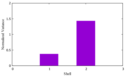
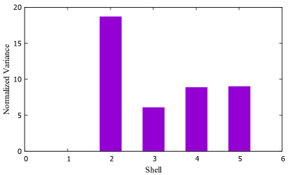
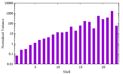
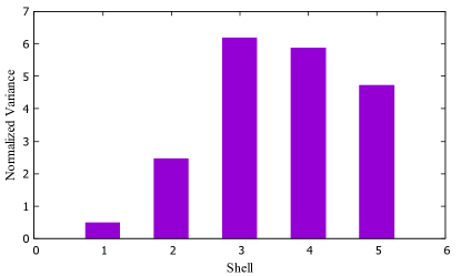
As mentioned in Section 2, k-shell centrality is one of the best-known methods to determine nodes’ influence, and various methods have been proposed based on it. Assigning the same k-shell index to the nodes with different degrees can be regarded as one of the issues in this centrality measure, as it leads to decreasing accuracy in nodes ranking. To demonstrate this issue, four indicative real world networks, Hamsterster (HMS) [15], Euroroad (EUR) [38], US Power grid (UGP) [43] and Chicago (CHG) [7] have been considered. The purpose of this study was to investigate the degree diversity of the nodes in the same shell. The results of this study are shown in Fig. 1. The Normalized Variance of nodes’ degree within each shell is reported in this figure. The normalized variance is calculated as follows: if nodes $\{v_{1},v_{2},...,v_{t}\}$ are in a shell then the variance of the degree of nodes, i.e. $d_{1},d_{2},...,d_{t}$, is first calculated, then the result is divided by the number of nodes, $t$.

As seen in Fig. 1, the same k-shell is assigned to nodes with different degrees; the degree of the nodes in each shell varies significantly. For example, in the HMS network, the value of the normalized variance of the degree of nodes located in shell 22 shows that nodes with significantly different degree values are assigned in the same shell. This observation suggests that the k-shell decomposition method cannot determine accurately the structural information of nodes with different features. Although the nodes closer to the core of the graph are more influential in comparison to the peripheral nodes, distinguishing the nodes located in each shell, based on their degree, can improve the ranking accuracy. Thus, in order to determine the spreading ability of nodes, degree and k-shell of the neighbours are considered simultaneously in this paper.

In other words, the idea is that nodes having neighbours that are located in shells closer to the core of the graph and with large degree values are more central. By considering the variation of k-shell and degree in the neighbourhood of a node, this can help determine the structural features of neighbours and distinguish the nodes located in the same shell but having different degrees. In brief, the variation between degree and k-shell of the first and second-order neighbours of each node can be used as a basis of a covariance approach to centrality and motivates the proposed measure.

4 The Details of the Proposed Method

In this section the details of the proposed method are discussed. A social network can be modelled as a graph $G=(V,E)$. The sets $V=\{v_{1},v_{2},\dots,v_{|V|}\}$, representing users, and $E=\{e_{1},e_{2},\dots,e_{|E|}\}$, representing the relations between users, are the sets of nodes and edges of the graph, respectively. $N_{z}$ is the set of neighbours of node $v_{z}$. The cardinality of this set shows the degree of the node, $d_{z}$.

4.1 Proposed Method

In the proposed method, we first define a measure, called Shell-Degree-Centrality (SDC), to determine the variation between degree and k-shell of the first- and second-order neighbours of each node. The Covariance Centrality (CVC) of each node is then calculated based on the value of neighbours’ SDC. Finally, the CVC of the neighbours is used to determine the Extended Covariance Centrality (ECVC) of each node, which indicates the spreading capability and rank of nodes in our proposed method. All this will be explained next.

In order to calculate the SDC of each node, two matrices $A^{(1)}(z)$ and $A^{(2)}(z)$ are first defined for each node $v_{z}$ to capture the properties of first-order and second-order neighbours, respectively. In these matrices, rows represent k-shell index and columns represent degree. The maximum k-shell and degree in the network are denoted by $s$ and $d$, respectively, hence each of these matrices has a size of $s\times d$. The value of each element of the matrix $A^{(r)}(z)$ is given by Eq. (1).

$$A_{ij}^{(r)}(z)=\frac{z_{ij}^{(r)}}{\sum_{i=1}^{s}{\sum_{j=1}^{d}{z_{ij}^{(r)}}}}$$ (1)

where $r$ is to differentiate between first-order neighbours ($r=1$) and second-order neighbours ($r=2$) of node $v_{z}$. In the equation, $z_{ij}^{(1)}$ is the number of the first-order neighbours of node $v_{z}$ which have k-shell=$i$ and degree=$j$. The value of $z_{ij}^{(1)}$ is calculated using Eq. (2).

$$z_{ij}^{(1)}=|\{v_{w}\mbox{ where }ks_{w}=i,d_{w}=j,v_{w}\in N_{z}\}|$$ (2)

$z_{ij}^{(2)}$ is also the number of the second-order neighbours of node $v_{z}$ which have k-shell=$i$ and degree=$j$. The value of $z_{ij}^{(2)}$ is calculated using Eq. (3).

$$z_{ij}^{(2)}=|\{v_{x}\mbox{ where }ks_{x}=i,d_{x}=j,v_{x}\in N_{w},v_{w}\in N_{z}\}|$$ (3)

Then, the covariance value of each matrix $A^{(1)}(z)$ and $A^{(2)}(z)$ is calculated; this is a value between $-1$ and $1$. If there is a direct relation between degree and k-shell in the neighbourhood of node $v_{z}$ the covariance takes a value close to 1. That is to say, if the value of degree increases by increasing k-shell in the neighbourhood of the node, the matrices have larger values of covariance, and the node is accordingly more influential. To calculate the covariance of matrix $A^{(r)}(z)$, Eq. (4) is used.

$$Cov(A^{(r)}(z))=E(A^{(r)}(z))-E(S^{(r)}(z))\cdot E(D^{(r)}(z))$$ (4)

where $S^{(r)}(z)$ and $D^{(r)}(z)$ are marginal distributions of matrix $A^{(r)}(z)$ and are calculated using Eqs. (5) and (6). In these equations $A_{ij}^{(r)}(z)$ is the entry of matrix $A^{(r)}(z)$ in row $i$ and column $j$.

$$S_{i}^{(r)}(z)=\sum_{j=1}^{d}A_{ij}^{(r)}\;\;i=1,...,s$$ (5)

$$D_{i}^{(r)}(z)=\sum_{j=1}^{s}A_{ji}^{(r)}\;\;i=1,...,d$$ (6)

In Eq. (4), $E(S^{(r)}(z))$ and $E(D^{(r)}(z))$ are the expectation of the marginal distribution $S^{(r)}(z)$ and $D^{(r)}(z)$, respectively. $E(A^{(r)}(z))$ is also the expectation of matrix $A^{(r)}(z)$. Their values are calculated using Eqs. (7) to (9).

$$E(S^{(r)}(z))=\sum_{i=1}^{s}\frac{i}{s}\,S_{i}^{(r)}(z)$$ (7)

$$E(D^{(r)}(z))=\sum_{i=1}^{d}\frac{i}{d}\,D_{i}^{(r)}(z)$$ (8)

$$E(A^{(r)}(z))=\sum_{i=1}^{s}\sum_{j=1}^{d}\frac{i}{s}\,\frac{j}{d}\,A_{ij}^{(r)}(z)$$ (9)

Then, the SDC value for node $v_{z}$ is calculated using Eq. (10), based on the values obtained for $Cov(A^{(1)}(z))$ and $Cov(A^{(2)}(z))$ from Eq. (4).

$$\begin{multlined}SDC(v_{z})=\frac{d_{z}}{d}\,(2+Cov(A^{(1)}(z)))+\\ \frac{d_{z}^{(2)}}{d^{(2)}}\,(2+Cov(A^{(2)}(z)))\end{multlined}SDC(v_{z})=\frac{d_{z}}{d}\,(2+Cov(A^{(1)}(z)))+\\ \frac{d_{z}^{(2)}}{d^{(2)}}\,(2+Cov(A^{(2)}(z)))$$ (10)

In this equation, $d_{z}^{(2)}=\sum_{v_{w}\in N_{z}}d_{w}$ is the second-order degree of node $v_{z}$, and $d^{(2)}$ is the maximum second-order degree in the network.

Algorithm 1 shows pseudo-code of the proposed method for calculating the SDC centrality of node $v_{z}$.

Data: Graph $G(V,E)$ and node $v_{z}$

Result: The value of SDC centrality of node $v_{z}$

1 set $r$=1 ;

2 calculate matrix $A^{(r)}(z)$ using Eq. (1);

3 calculate the marginal distributions $S^{(r)}(z)$ and $D^{(r)}(z)$ using Eqs. (5) and (6), respectively;

4 calculate $E(S^{(r)}(z))$, $E(D^{(r)}(z))$ and $E(A^{(r)}(z))$, using Eqs. (7), (8) and (9), respectively;

5 calculate $Cov(A^{(r)}(z))$ using Eq. (4);

6 set $r$=2 and repeat steps 2 to 5;

calculate SDC($v_{z}$) using Eq. (10)

Algorithm 1 SDC calculation for $v_{z}$

Although SDC centrality can be used to determine the spreading capability of nodes too, considering the centrality of the neighbours increases the accuracy of this determination [23]. To achieve this, we cumulatively sum up the centrality of neighbours (indirectly up to second-order neighbours) using Eqs. (11) and (12), where the Covariance Centrality (CVC) and the Extended Covariance Centrality (ECVC) for node $v_{z}$ are defined based on the SDC of its neighbours.

$$CVC(v_{z})=\sum_{V_{w}\in N_{i}}SDC(v_{w})$$ (11)

$$ECVC(v_{z})=\sum_{V_{w}\in N_{i}}CVC(v_{w})$$ (12)

We calculate the ECVC of every node of the network to determine a node’s spreading ability and produce a ranking list that ranks nodes in descending order of their influence. Algorithm 2 shows the pseudo-code of the proposed method to rank the nodes.

Data: Graph $G(V,E)$

Result: Ranking list (list of nodes in descending order of influence)

1 calculate SDC($v_{z}$) for each $v_{z}\in V$ using Algorithm 1;

2 calculate CVC($v_{z}$) for each $v_{z}\in V$ using Eq. (11);

3 calculate ECVC($v_{z}$) for each $v_{z}\in V$ using Eq. (12);

rank the nodes in descending order according to their ECVC value.

Algorithm 2 ECVC ranking pseudo-code

The time complexity of Algorithm 1 can be analysed as follows. The calculation of the $A^{(1)}(z)$ matrix for each node $v_{z}$ needs $O(\langle d\rangle)$, where $\langle d\rangle$ is the average degree of nodes. In line 3 of the algorithm, it takes $O(s)$ and $O(d)$ to calculate $S^{(1)}$ and $D^{(1)}$, respectively. The calculation of Eqs. (7), (8) and (9) in line 4 of the algorithm needs $O(s)$, $O(d)$, and $O(s\times d)$, respectively. Line 5 is $O(1)$. These steps must be repeated for $r=2$. The complexity is the same as $r=1$ with the exception of line 2 which is $O(\langle d^{(2)}\rangle)$; $\langle d^{(2)}\rangle$ is the average value of second-order degree of nodes. Thus, the time complexity of Algorithm 1 is $O(\langle d\rangle+\langle d^{(2)}\rangle+2\times(2s+2d+s\times d+1))\in O(\langle d^{(2)}\rangle)$. In Algorithm 2, the SDC centrality of every node must be calculated using Algorithm 1, so it has time order $O(|V|\times\langle d^{(2)}\rangle)$. The calculation of CVC and ECVC have complexity $O(\langle d\rangle)$ and $O(\langle d^{(2)}\rangle)$, respectively. The time complexity of the k-shell algorithm to determine the shells is $O(|E|)$ [1]. Thus, the total complexity of the proposed method is $O(|E|+|V|\times\langle d^{(2)}\rangle+\langle d\rangle+\langle d^{(2)}\rangle)\in O(|E|+|V|\times\langle d^{(2)}\rangle)$.

Figure 2: An example network

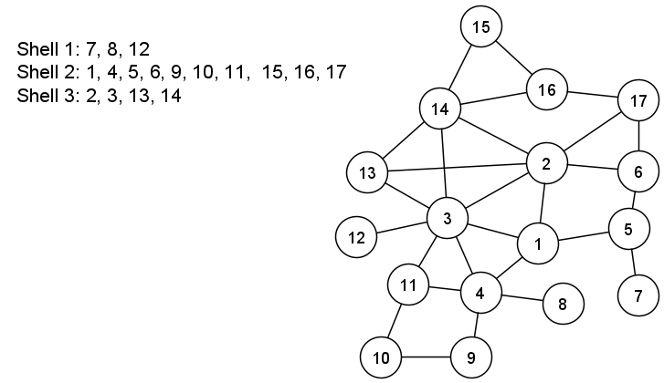
4.2 An example

As an example, to understand the proposed method, consider Fig. 2. In this graph the maximum shell, $s$, and maximum degree, $d$ are 3 and 7, respectively. The nodes located in each shell are shown in the figure. We will show how to calculate the value of ECVC centrality for node 2, $v_{2}$.

Node 2, $v_{2}$, has 6 neighbours, i.e $N_{2}=\{v_{1},v_{3},v_{6},v_{13},v_{14},v_{17}\}$ and $d_{2}=6$. The matrix $A^{(1)}(2)$ for this node is calculated as follows.

$$A^{(1)}(2)=\begin{pmatrix}\frac{0}{6}&\frac{0}{6}&\frac{0}{6}&\frac{0}{6}&\frac{0}{6}&\frac{0}{6}&\frac{0}{6}\\ &&&&&&\\ \frac{0}{6}&\frac{0}{6}&\frac{2}{6}&\frac{1}{6}&\frac{0}{6}&\frac{0}{6}&\frac{0}{6}\\ &&&&&&\\ \frac{0}{6}&\frac{0}{6}&\frac{1}{6}&\frac{0}{6}&\frac{1}{6}&\frac{0}{6}&\frac{1}{6}\\ \end{pmatrix}$$

The value of the element in row $i$ and column $j$ of the matrix indicates what is the proportion of neighbours with k-shell $i$ and degree $j$ that node 2 has. Consider for instance the element in row 2 and column 3 of the matrix. The value of $\frac{2}{6}$ means that out of a total of six neighbours $v_{2}$ has two neighbours with k-shell 2 and degree 3; indeed, these nodes are $v_{6}$ and $v_{17}$.

We use Eq. (5) to calculate the vector $S^{(1)}(2)$. For example, the value of the third element of $S^{(1)}(2)$ is calculated as $S_{3}^{(1)}(2)=A_{3,1}^{(1)}(2)+A_{3,2}^{(1)}(2)+A_{3,3}^{(1)}(2)+A_{3,4}^{(1)}(2)+A_{3,5}^{(1)}(2)+A_{3,6}^{(1)}(2)+A_{3,7}^{(1)}(2)=\frac{0}{6}+\frac{0}{6}+\frac{1}{6}+\frac{0}{6}+\frac{1}{6}+\frac{0}{6}+\frac{1}{6}=\frac{3}{6}$. The value of the other entries of $S^{(1)}(2)$ is calculated similarly. Hence, $S^{(1)}(2)$ is given by

$$S^{(1)}(2)=\begin{pmatrix}\frac{0}{6}&\frac{3}{6}&\frac{3}{6}\\ \end{pmatrix}$$

We use Eq. (6) to calculate the vector $D^{(1)}(2)$. For example, the value of the fourth element of $D^{(1)}(2)$ is calculated as $D_{4}^{(1)}(2)=A_{1,4}^{(1)}(2)+A_{2,4}^{(1)}(2)+A_{3,4}^{(1)}(2)=\frac{0}{6}+\frac{1}{6}+\frac{0}{6}=\frac{1}{6}$. Overall, $D^{(1)}(2)$ is given by

$$D^{(1)}(2)=\begin{pmatrix}\frac{0}{6}&\frac{0}{6}&\frac{3}{6}&\frac{1}{6}&\frac{1}{6}&\frac{0}{6}&\frac{1}{6}\\ \end{pmatrix}$$

The expectation of the marginal distribution $S^{(1)}(2)$ and $D^{(1)}(2)$ and matrix $A^{(1)}(2)$ is calculated using Eqs. (7,8,9) as

$$\begin{split}E(S^{(1)}(2))=\frac{1}{3}\cdot\frac{0}{6}+\frac{2}{3}\cdot\frac{3}{6}+\frac{3}{3}\cdot\frac{3}{6}\cong 0.83\end{split}$$

$$\begin{split}E(D^{(1)}(2))\!=\!\frac{1}{7}\!\cdot\!\frac{0}{6}\!+\!\frac{2}{7}\!\cdot\!\frac{0}{6}\!+\!\frac{3}{7}\!\cdot\!\frac{3}{6}\!+\!\frac{4}{7}\!\cdot\!\frac{1}{6}\!+\!\frac{5}{7}\!\cdot\!\frac{1}{6}\!+\!\frac{6}{7}\!\cdot\!\frac{0}{6}\!+\!\frac{7}{7}\!\cdot\!\frac{1}{6}\cong 0.60\end{split}$$

$$\begin{split}E(A^{(1)}(2))=\frac{1}{3}\cdot\frac{1}{7}\cdot A_{1,1}^{(1)}(2)+\frac{1}{3}\cdot\frac{2}{7}\cdot A_{1,2}^{(1)}(2)+\frac{1}{3}\cdot\frac{3}{7}\cdot A_{1,3}^{(1)}(2)+\dots=\\ =\frac{1}{3}\cdot\frac{1}{7}\cdot\frac{0}{6}+\frac{1}{3}\cdot\frac{2}{7}\cdot\frac{0}{6}+\frac{1}{3}\cdot\frac{3}{7}\cdot\frac{0}{6}+\dots\cong 0.52\end{split}$$

The value of $Cov(A^{(1)}(2))$ is calculated using Eq. (4) as

$$\begin{split}Cov(A^{(1)}(2))=E(A^{(1)}(2))-E(S^{(1)}(2))\cdot E(D^{(1)}(2))\cong 0.52-0.83\cdot 0.60\cong 0.02\end{split}$$

The same process is repeated for the second-order neighbours of $v_{2}$ and the value of $Cov(A^{(2)}(2))$ obtained is $Cov(A^{(2)}(2))\cong 0.04$. The value of the SDC centrality of node 2, $v_{2}$, is calculated using Eq. (10) as

$$\begin{split}SDC(2)=&\frac{6}{7}\cdot(2+Cov(A^{(1)}(2)))+\frac{25}{27}\cdot(2+Cov(A^{(2)}(2)))\cong\\ \cong&\frac{6}{7}\cdot(2+0.02)+\frac{25}{27}\cdot(2+0.04)\cong 3.62\end{split}$$

The value of SDC centrality is similarly calculated for all nodes, and then the CVC centrality of node 2, $v_{2}$, is obtained using Eq. (11) as

$$\begin{split}CVC(2)=SDC(1)+SDC(3)+SDC(6)+SDC(13)+SDC(14)+SDC(17)\cong\\ \cong 2.75+4.08+1.78+2.21+3.03+1.77\cong 15.61\end{split}$$

After the calculation of the CVC centrality for all nodes, the value of ECVC centrality of node 2, $v_{2}$, is obtained using Eq. (12) as

$$\begin{split}ECVC(2)=CVC(1)+CVC(3)+CVC(6)+CVC(13)+CVC(14)+CVC(17)\cong\\ \cong 11.91+17.10+6.86+10.72+12.70+7.01\cong 66.31.\end{split}$$

5 Experimental Results

This section evaluates the performance of the proposed method, ECVC (as well as the measures that compose it, SDC and CVC), in comparison with another eleven centrality measures that can be used to identify and rank influential nodes. The eleven methods are: k-shell (KS) [14], degree (D) [8], mixed degree decomposition (MDD) [52], extended neighbourhood coreness (Cnc+) [1], k-shell iteration factor (KS-IF) [42], degree and importance of links (DIL) [21], Mixed Core, Semi-local Degree and Weighted Entropy (MCDE) [37], link significance (LS) [40], hierarchical k-shell (HKS) [47], diversity-strength ranking (DSR) [50], and weighted k-shell degree (WKD) [30].

A set of twelve real and two artificial (LFR-200 and LFR-1000) networks are used, as shown in Table 1. The real world networks include: Karate club(KRT) [46], Dolphins (DLN) [26], Jazz musician (JZM) [11], Netsciense (NTS) [34], Facebook Food (FFD) [6], Euroroad (EUR) [38], Euroroad (EUR) [38], Chicago (CHG) [7], Chicago (CHG) [7], Hamsterster (HMS) [15], Ego-Facebook (FCB) [29], US Power grid (UPG) [43], LastFM (LFM) [35] and Pretty Good Privacy (PGP) [2]. For each network, the table shows: number of nodes $(|V|)$, number of edges $(|E|)$, maximum degree $(MD)$, average degree of nodes $(\langle d\rangle)$, average second-order degree of nodes $(\langle d^{(2)}\rangle)$ and average clustering coefficient $(CC)$. The Lancichinetti–Fortunato–Radicchi (LFR) benchmark [16] is used to generate the artificial networks. LFR is able to generate an artificial network with a set of defined parameters, such as, number of nodes $(|V|)$, average degree of nodes $(\langle d\rangle)$, mixing parameter of the community structure $(\mu)$, and power-law of the degree distribution $(\gamma)$. These parameters are set as $|V|=200$, $\langle d\rangle=5$, $\gamma=2$, and $\mu=0.2$ to generate LFR-200, and they are set as $|V|=1000$, $\langle d\rangle=10$, $\gamma=2$, and $\mu=0.2$ to generate LFR-1000.

Two different criteria are used to evaluate the ranking list produced by the different methods for different networks. The first criterion is discrimination of the nodes with different spreading ability, which is the capability to differentiate between nodes according to their influence. The second criterion is accuracy (or correctness), which assesses the ranking list and the nodes in terms of their spreading ability using a standard model that simulates the spreading process. An experiment is also dedicated to evaluating the average running time of all the methods.

(a) FCB

(b) UPG

(c) LFM

(d) PGP

Figure 3: The number of nodes ($NN$) in different ranks of $R$ by various methods in FCB, UPG, LFM and PGP networks

5.1 Discrimination

The discrimination of the ranking list $R$ produced by different methods is investigated in this section. A distinct metric (DM) function [10] is applied for this purpose. The value of the DM function for the list $R$ is calculated using Eq. (13). The value of DM is in the interval $(0,1]$; a larger value shows better discrimination in $R$.

$$DM(R)=\frac{\mbox{number of distinct ranks}}{|V|}$$ (13)

A rank refers to a group of nodes with the same influence value (as computed by some centrality measure). Clearly, if all nodes have a different value maximum discrimination is achieved (DM=1) [10].

The results obtained are shown in Table 2. ECVC considers the relation between degree and k-shell for nodes’ neighbours to discriminate the spreading ability of nodes which are located in the same shell. As seen from the table, ECVC has overall better distinction in comparison to other methods. ECVC significantly outperforms all methods in larger networks. In three relatively small networks, such as NTS, L1000 and FCB, DSR performs better than ECVC but this is by a small margin. Overall ECVC shows better properties than other measures.

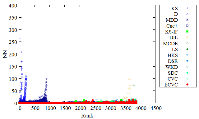
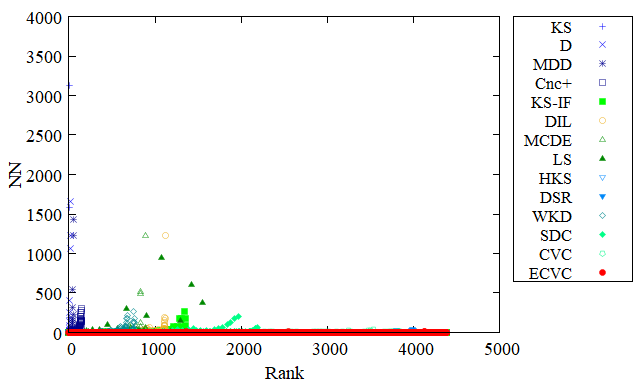
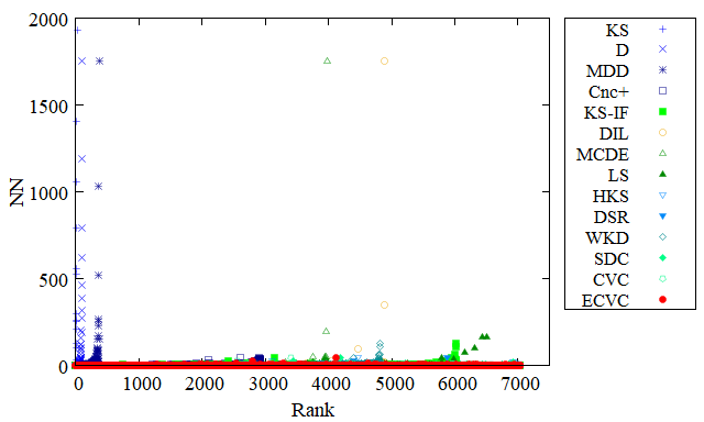
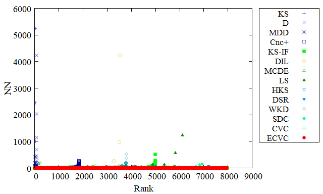
For a better evaluation of the discrimination ability of the proposed method, the number of nodes (NN) in different ranks of the ranking list $R$ is investigated in the next experiment of this section. Fig. 3 shows the obtained results of the experiment using the four largest networks, FCB, UPG, LFM, PGP, which have different features. It can be seen from Fig. 3 that ECVC assigns a small number of nodes to the same rank. This means that nodes are ranked in more ranks by ECVC as opposed to other methods, something that leads to better discrimination, especially in large networks.

5.2 Accuracy

In this section, the accuracy of the ranking list $R$ produced by different methods is evaluated using three sets of experiments. To do so, a susceptible-infected-recovered (SIR) model [31, 32] is used to simulate the spreading process in the real world and determine the ground-truth influence of nodes. The real influence ranking list $(\sigma)$ is determined based on the ground-truth influence of nodes.

SIR is one of the epidemic diffusion models which has been widely used in research [1, 17, 40, 50] to simulate spreading process and generate a real influence ranking list. In this model, each node can be in one of susceptible, infected, or recovered states. Node $v_{i}$ is initially considered as an infected node and all other nodes are considered as susceptible. In each timestamp, each infected node is changed to recovered state after its attempt to infect each susceptible neighbour with infection probability $\beta$. This process continues until there is not any infected node in the network. The number of recovered nodes is considered as ground-truth influence of node $v_{i}$. This epidemic process is repeated for every node $(i=1,\dots,|V|)$ and the real influence ranking list $(\sigma)$ is accordingly determined. In our experiments, in line with other studies [1, 30, 24, 50], to increase the accuracy in determining $\sigma$, the SIR model is repeated 1000 times for each node and the average value of the number of recovered nodes is considered as influence. The value of $\beta$ must be chosen so that it is slightly greater than the infection threshold $\beta_{th}=\frac{\langle d\rangle}{\langle d^{(2)}\rangle}$ [1], where $\langle d\rangle$ and $\langle d^{(2)}\rangle$ are the average of first- and second-order degrees of the network nodes, respectively. The values of $\beta_{th}$ and $\beta$ considered for each network are given in Table 3.

The Kendall tau correlation coefficient $(\tau)$ [13] is employed to calculate the correlation between the ranking lists $R$ and $\sigma$ for each different method. A higher value of correlation between $\sigma$ and $R$ shows better accuracy of the ranking list $R$. For this purpose, concordant and discordant pair sets between $R$ and $\sigma$ are determined. Suppose that $(\sigma_{1},R_{1}),(\sigma_{2},R_{2}),\dots,(\sigma_{n},R_{n}),$ is a set of pair ranks in $R$ and $\sigma$. If $(\sigma_{i}>\sigma_{j}\mbox{ and }R_{i}>R_{j})$ or $(\sigma_{i}<\sigma_{j}\mbox{ and }R_{i}<R_{j})$ then $(\sigma_{i},R_{i})$ and $(\sigma_{j},R_{j})$ are considered as concordant pairs. Conversely, they are considered as discordant pairs if $(\sigma_{i}>\sigma_{j}\mbox{ and }R_{i}<R_{j})$ or $(\sigma_{i}<\sigma_{j}\mbox{ and }R_{i}>R_{j})$. The Kendal tau correlation coefficient, $\tau(\sigma,R)$, is calculated with the help of Eq. (14) and it is a real number in [$-1,+1$]. A value of zero indicates no correlation between the lists, whereas values closer to 1 show high positive correlation and values closer to $-1$ show high negative correlation.

$$\tau(\sigma,R)=\frac{n_{c}-n_{d}}{\frac{1}{2}(n)(n-1)}$$ (14)

(a) FFD

(b) NTS

(c) CHG

(d) EUR

Figure 4: The effect of varying the value of the infection probability on the accuracy of different methods using the FFD, NTS, CHG, and EUR networks

(a) FCB

(b) UPG

(c) LFM

(d) PGP

Figure 5: The value of RBO for different methods using the FCB, UPG, LFM and PGP networks

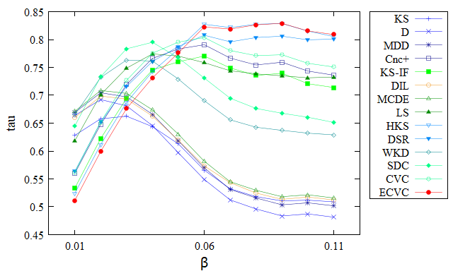
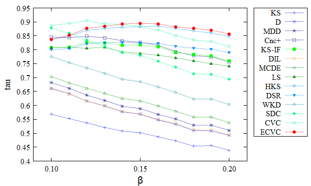
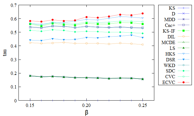
The first experiment compares ECVC, SDC, CVC and the eleven different methods from the literature, which are used to determine a ranking list $R$; then, the Kendall tau correlation coefficient $(\tau)$ between $R$ and $\sigma$ is calculated. Table 4 shows the value of $\tau$ for all networks and methods. It can be seen from Table 4 that ECVC outperforms other methods most of the time. HKS has higher accuracy than ECVC for the KRT, FFD and UPG networks and equal accuracy for L1000 but for all other networks ECVC has the highest accuracy. This is because degree and k-shell of neighbours are concurrently taken into account: nodes whose neighbours have high degree and appropriate topological location are considered as influential nodes by ECVC. Focusing on the three methods proposed in this paper, ECVC, SDC, and CVC, it can be seen that ECVC outperforms the other two methods, except in the case of the KRT and JZM networks. This is because these two networks are small, yet the average second-order degree is larger than the number of nodes, which suggests that ECVC may overestimate structural information.

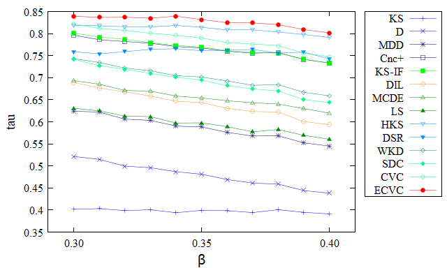
In the second experiment, we assess the effect of varying the infection probability on the accuracy of ECVC. For this purpose, this value is varied from $\beta-0.05$ to $\beta+0.05$ in steps of 0.01 (a total of 11 different values). The ranking list $\sigma$ is determined using the SIR model. The Kendall tau correlation coefficient between $\sigma$ and ranking list $R$ is then calculated. The results obtained using four representative networks, FFD, NTS, CHG, and EUR, are shown in Fig. 4. As the infection probability increases, the message can spread to farther distances. Then, the first and second-order neighbours play a more important role in the spreading process. When the value of $\beta$ is very small, second-order neighbours become less important in the spreading process. Thus, for small values of $\beta$, methods that rely on first-order neighbours to determine the spreading ability of nodes are reasonably accurate, something that can be observed in Fig. 4a. As the value of $\beta$ increases, the second-order neighbours play a more important role in the spreading process. In this case, methods relying on first-order neighbours have lower accuracy whereas the accuracy of methods that take additional information in the neighbourhood into account, increases. As seen in Fig. 4, ECVC has the highest accuracy and outperforms all other methods in all cases, except for small values of $\beta$ in Fig. 4a, for the reasons already discussed.

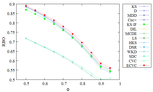
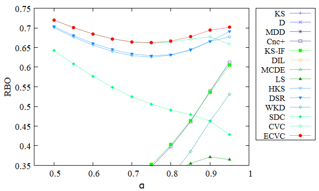
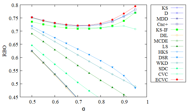
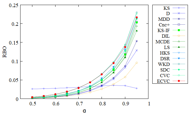
The third experiment is dedicated to the evaluation of the accuracy of the proposed method with respect to top-ranks. This is of interest as most influential nodes belong to top-ranks in the ranking list (recall the definition of rank in the description of Eq. (13). For this purpose, the rank-biased overlap (RBO) function [44] is employed to assess the overlap of top-ranks in the real influence ranking list, $\sigma$ with top-ranks in the ranking list, $R$, produced by each method. The value of RBO is calculated as in Eq. (15).

$$RBO(\sigma,R,\alpha)=(1-\alpha)\sum_{f=1}^{n}\alpha^{f-1}A(\sigma,R,f)$$ (15)

where $n$ is the maximum number of distinct ranks in the ranking lists $\sigma$ and $R$. The parameter $\alpha$ can take values between 0 and 1. A lower value of $\alpha$ gives higher importance to top-ranks in the ranking list $R$. $A(\sigma,R,f)$ is the amount of overlap between the first $f$ top-ranks of the lists and is calculated using Eq. (16). In this equation, $\sigma(f)$ and $R(f)$ are the set of nodes in the $f$ top-ranks in lists $\sigma$ and $R$, respectively.

$$A(\sigma,R,f)=\frac{|\sigma(f)\cap R(f)|}{|\sigma(f)\cup R(f)|}$$ (16)

The value of RBO function is in [0, 1]. A higher value of this function shows more overlap between the top-ranks of the lists, and, accordingly, a higher accuracy of the top-ranks of list $R$. The results for this experiment, using the four largest networks FCB, UPG, LFM and PGP, are shown in Fig. 5. A lower value of $\alpha$ gives greater weight to the top ranks in the ranking list. This means that a downward trend in Fig. 5 suggests that the ranking list has greater accuracy for top ranks but its accuracy decreases going toward the lower ranks. Conversely, an upward trend suggests less accuracy in top ranks but the accuracy increases as we give more weight to the lower ranks. As can be seen from Fig. 5, ECVC outperforms all other methods consistently with the only exception being the PGP network. This may be because, in this network, nodes are ranked in a relatively small number of ranks with many nodes in each rank, something that may potentially decrease the estimated overlap according to Eq. 16.

5.3 Running Time

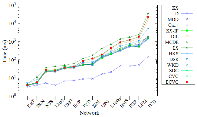
This section is dedicated to the evaluation of the running time of all different methods. For this purpose, each method has been executed 100 times with each network and the average running time is reported in Fig. 6. The x-axis lists the networks in ascending order of the number of edges. As seen in the figure, the running time of methods increases as the number of edges increases. LS and ECVC have the first and second highest running time followed by DIL, however, all methods (with the only exception of the rather simple D) appear to perform within one order of magnitude. As expected, the core of ECVC, which is SDC, performs better than ECVC. In fact, SDC’s running time does not appear to have a difference in performance compared to the majority of other methods.

Figure 6: Running time (in seconds) of the different methods

6 Summary

The problem of identifying users’ influence and ranking them in social networks has attracted considerable attention in various research studies; different methods have been proposed for it. The distance to the core of graph is an effective criterion in users’ influence. This observation motivated this paper, which has taken into account k-shell and degree of first- and second-order neighbours to propose a composite centrality measure, based on covariance, to determine the importance of each node. A set of experiments were conducted to evaluate the discrimination ability and accuracy of the proposed method. The results obtained showed the superiority of the proposed method in comparison to other similar methods. In future work, somebody may investigate different weights for degree and k-shell and additional experiments. Additional work may also consider the relationship between other structural features and the definition of a centrality measure. Finally, it would be interesting to modify the proposed method so that it can be applied in weighted networks.

Table 1: Properties of the networks used in experiments

Network	$|V|$	$|E|$	MD	$\langle d\rangle$	$\langle d^{(2)}\rangle$	$CC$
Karate club (KRT)	34	78	17	4.5882	35.6741	0.5706
Dolphins (DLN)	62	159	12	5.1290	34.9032	0.2589
Jazz musician (JZM)	198	2,742	100	27.6970	1070.2400	0.6174
LFR-200 (L200)	200	1,052	16	10.5200	116.6800	0.4335
Netsciense (NTS)	379	914	34	4.8232	38.686	0.7412
Facebook Food (FFD)	620	2,092	132	6.74516	134.319	0.3309
LFR-1000 (L1000)	1,000	10,610	98	21.2200	797.5360	0.4232
Euroroad (EUR)	1,174	1,417	10	2.4140	7.2042	0.0167
Chicago (CHG)	1,467	1,298	12	1.7696	9.5801	0.0000
Hamsterster (HMS)	2,426	16,631	273	13.7110	582.9300	0.5380
Ego-Facebook (FCB)	4,039	88,234	1392	43.6910	4656.3200	0.6055
US Power grid (UPG)	4,941	6,594	19	2.6691	10.3327	0.0801
LastFM (LFM)	7,624	27,806	324	7.2943	185.4370	0.2194
Pretty Good Privacy (PGP)	10,680	24,316	205	4.5536	85.9762	0.2659

Table 2: DM value for ranking list R by different methods

network	KS	D	MDD	Cnc+	KS-IF	DIL	MCDE	LS	HKS	DSR	WKD	SDC	CVC	ECVC
KRT	0.1176	0.3235	0.4412	0.7647	0.7941	0.7059	0.7059	0.7941	0.7941	0.7647	0.7941	0.7941	0.7941	0.8529
DLN	0.0645	0.1935	0.3710	0.8226	0.9677	0.8710	0.8710	0.9516	0.9677	0.9677	0.9032	0.9677	0.9677	0.9677
JZM	0.1061	0.3131	0.6263	0.9646	0.9646	0.9343	0.9444	0.9747	0.9646	0.9697	0.9697	0.9646	0.9747	0.9697
L200	0.0100	0.0250	0.0850	0.3150	0.7750	0.8000	0.5700	0.9750	0.9500	0.9950	0.4600	0.5050	0.9450	0.9950
NTS	0.0211	0.0554	0.1425	0.4855	0.6807	0.3272	0.5251	0.7071	0.6913	0.7150	0.6491	0.7018	0.7071	0.7018
FFD	0.0177	0.0661	0.1790	0.6968	0.8355	0.6710	0.5516	0.8371	0.4648	0.4681	0.7823	0.8903	0.9048	0.9048
L1000	0.0120	0.0430	0.1770	0.8670	0.9870	0.9850	0.9510	0.9960	0.9970	0.9990	0.9490	0.9980	0.9980	0.9980
EUR	0.0017	0.0077	0.0187	0.0451	0.3101	0.2078	0.1925	0.1635	0.5954	0.7802	0.1397	0.3296	0.6899	0.8722
CHG	0.0007	0.0075	0.0109	0.0204	0.0416	0.2154	0.0075	0.0075	0.0723	0.0688	0.0307	0.0300	0.0654	0.0995
HMS	0.0095	0.0458	0.1467	0.6393	0.6744	0.6195	0.6179	0.6950	0.6810	0.6962	0.6686	0.6814	0.7042	0.7045
FCB	0.0238	0.0562	0.2238	0.9468	0.9549	0.9044	0.9369	0.9579	0.9577	0.9591	0.9542	0.9567	0.9582	0.9574
UPG	0.0010	0.0032	0.0105	0.0306	0.2740	0.2283	0.1813	0.3153	0.3982	0.8089	0.01540	0.4426	0.7766	0.8875
LFM	0.0026	0.0129	0.0485	0.3831	0.7905	0.6422	0.5215	0.8538	0.9136	0.9079	0.6321	0.9088	0.9218	0.9226
PGP	0.0024	0.0078	0.0287	0.1722	0.4677	0.3291	0.3497	0.5724	0.6766	0.6744	0.3546	0.6495	0.7333	0.7450

Table 3: The values of the infection threshold $\beta_{th}$ and infection probability $\beta$ considered for different networks

Network	$\beta_{th}$	$\beta$	Network	$\beta_{th}$	$\beta$
KRT	0.129	0.15	EUR	0.333	0.35
DLN	0.147	0.15	CHG	0.185	0.2
JZM	0.026	0.05	HMS	0.024	0.03
L200	0.18	0.2	FCB	0.009	0.01
NTS	0.125	0.15	UPG	0.258	0.3
FFD	0.0502	0.06	LFM	0.039	0.04
L1000	0.053	0.06	PGP	0.053	0.1

Table 4: Value of Kendall tau correlation coefficient between $R$ and $\sigma$ for different networks and methods

Network	KS	D	MDD	Cnc+	KS-IF	DIL	MCDE	LS	HKS	DSR	WKD	SDC	CVC	ECVC
KRT	0.5544	0.6809	0.7041	0.7647	0.7291	0.7059	0.7112	0.7504	0.7754	0.7504	0.7469	0.7718	0.7718	0.7647
DLN	0.5791	0.7721	0.8038	0.8847	0.8445	0.8096	0.8075	0.8377	0.9112	0.8995	0.8255	0.8477	0.8837	0.9143
JZM	0.7718	0.8634	0.8907	0.9219	0.8754	0.844	0.9291	0.8404	0.9179	0.9444	0.9203	0.9174	0.9485	0.9294
L200	0.047	0.5895	0.683	0.8451	0.8320	0.6507	0.6975	0.5800	0.8107	0.7386	0.7762	0.7832	0.8712	0.8847
NTS	0.5018	0.5681	0.5886	0.8263	0.8171	0.5692	0.6159	0.7870	0.8823	0.8243	0.6852	0.7794	0.8830	0.8952
FFD	0.5657	0.5490	0.5699	0.7907	0.7704	0.5733	0.5817	0.7585	0.8272	0.8077	0.6903	0.7309	0.8036	0.8226
L1000	0.5929	0.5076	0.5479	0.7792	0.7647	0.5092	0.6078	0.7292	0.7850	0.7584	0.7134	0.7148	0.7794	0.7850
EUR	0.3993	0.4811	0.5884	0.7673	0.7697	0.6436	0.6540	0.5976	0.8142	0.7611	0.7015	0.6945	0.7900	0.8318
CHG	0.0000	0.1657	0.1669	0.5433	0.5669	0.4194	0.1681	0.1657	0.5941	0.4618	0.5414	0.5065	0.5752	0.6125
HMS	0.6836	0.6959	0.7007	0.8266	0.8245	0.7142	0.7085	0.8214	0.8347	0.8047	0.7730	0.7905	0.8360	0.8366
FCB	0.6970	0.6659	0.6844	0.8599	0.8501	0.6657	0.6933	0.7634	0.8554	0.7743	0.7569	0.7646	0.8288	0.8624
UPG	0.3359	0.4715	0.5071	0.7147	0.7246	0.5134	0.5447	0.5047	0.7974	0.7262	0.6196	0.6377	0.7507	0.7972
LFM	0.6161	0.5897	0.6036	0.8370	0.8104	0.5948	0.6270	0.7762	0.8537	0.8150	0.7455	0.7409	0.8245	0.8560
PGP	0.4073	0.4252	0.4361	0.7144	0.6821	0.4286	0.4490	0.6798	0.7344	0.7199	0.6214	0.5736	0.6856	0.7348

References

- [1] Joonhyun Bae and Sangwook Kim “Identifying and ranking influential spreaders in complex networks by neighborhood coreness” In Physica A: Statistical Mechanics and its Applications 395 Elsevier, 2014, pp. 549–559
- [2] Marián Boguñá, Romualdo Pastor-Satorras, Albert Díaz-Guilera and Alex Arenas “Models of social networks based on social distance attachment” In Physical Review E 70 American Physical Society, 2004, pp. 056122
- [3] Stephen P Borgatti and Martin G Everett “Models of core/periphery structures” In Social Networks 21.4 Elsevier, 2000, pp. 375–395
- [4] Thang N. Dinh, Dung T. Nguyen and My T. Thai “Cheap, Easy, and Massively Effective Viral Marketing in Social Networks: Truth or Fiction?” In Proceedings of the 23rd ACM Conference on Hypertext and Social Media, 2012, pp. 165–174
- [5] Pedro Domingos and Matt Richardson “Mining the Network Value of Customers” In Proceedings of the 7th ACM SIGKDD International Conference on Knowledge Discovery and Data mining, 2001, pp. 57–66
- [6] Jordi Duch and Alex Arenas “Community detection in complex networks using extremal optimization” In Physical Review E 72.2 APS, 2005, pp. 027104
- [7] R Eash, K Chon, Y Lee and D Boyce “Equilibrium traffic assignment on an aggregated highway network for sketch planning” In Transportation Research 13, 1979, pp. 243–257
- [8] Linton C Freeman “Centrality in social networks conceptual clarification” In Social Networks 1.3 North-Holland, 1978, pp. 215–239
- [9] Linton C. Freeman “A Set of Measures of Centrality Based on Betweenness” In Sociometry 40.1 [American Sociological Association, Sage Publications, Inc.], 1977, pp. 35–41
- [10] Shuai Gao et al. “Ranking the spreading ability of nodes in complex networks based on local structure” In Physica A: Statistical Mechanics and its Applications 403 Elsevier, 2014, pp. 130–147
- [11] Pablo M Gleiser and Leon Danon “Community structure in jazz” In Advances in Complex Systems 6.04 World Scientific, 2003, pp. 565–573
- [12] David Kempe, Jon Kleinberg and Éva Tardos “Maximizing the Spread of Influence through a Social Network” In Proceedings of the Ninth ACM SIGKDD International Conference on Knowledge Discovery and Data Mining, 2003, pp. 137–146
- [13] Maurice G Kendall “A new measure of rank correlation” In Biometrika 30.1/2 JSTOR, 1938, pp. 81–93
- [14] Maksim Kitsak et al. “Identification of influential spreaders in complex networks” In Nature Physics 6.11 Nature Publishing Group, 2010, pp. 888
- [15] Jérôme Kunegis “KONECT: The Koblenz Network Collection” In Proceedings of the 22nd International Conference on World Wide Web, 2013, pp. 1343–1350
- [16] Andrea Lancichinetti, Santo Fortunato and Filippo Radicchi “Benchmark graphs for testing community detection algorithms” In Physical Review E 78.4 APS, 2008, pp. 046110
- [17] Chao Li, Li Wang, Shiwen Sun and Chengyi Xia “Identification of influential spreaders based on classified neighbors in real-world complex networks” In Applied Mathematics and Computation 320 Elsevier, 2018, pp. 512–523
- [18] Mengtian Li et al. “Identifying and ranking influential spreaders in complex networks by combining a local-degree sum and the clustering coefficient” In International Journal of Modern Physics B 32.06 World Scientific, 2018, pp. 1850118
- [19] W. Li, Q. Bai, M. Zhang and T.. Nguyen “Automated Influence Maintenance in Social Networks: An Agent-based Approach” In IEEE Transactions on Knowledge and Data Engineering 31.10, 2019, pp. 1884–1897
- [20] Yuchen Li, Ju Fan, Yanhao Wang and Kian-Lee Tan “Influence maximization on social graphs: A survey” In IEEE Transactions on Knowledge and Data Engineering 30.10 IEEE, 2018, pp. 1852–1872
- [21] Jun Liu et al. “Evaluating the importance of nodes in complex networks” In Physica A: Statistical Mechanics and its Applications 452 Elsevier, 2016, pp. 209–219
- [22] Qiang Liu et al. “Leveraging local h-index to identify and rank influential spreaders in networks” In Physica A: Statistical Mechanics and its Applications 512 Elsevier, 2018, pp. 379–391
- [23] Ying Liu, Ming Tang, Tao Zhou and Younghae Do “Identify influential spreaders in complex networks, the role of neighborhood” In Physica A: Statistical Mechanics and its Applications 452 Elsevier, 2016, pp. 289–298
- [24] Linyuan Lü, Tao Zhou, Qian-Ming Zhang and H Eugene Stanley “The H-index of a network node and its relation to degree and coreness” In Nature Communications 7 Nature Publishing Group, 2016, pp. 10168
- [25] Linyuan Lü et al. “Vital nodes identification in complex networks” In Physics Reports 650 Elsevier, 2016, pp. 1–63
- [26] David Lusseau et al. “The bottlenose dolphin community of Doubtful Sound features a large proportion of long-lasting associations” In Behavioral Ecology and Sociobiology 54.4 Springer, 2003, pp. 396–405
- [27] Giridhar Maji, Sharmistha Mandal and Soumya Sen “A systematic survey on influential spreaders identification in complex networks with a focus on K-shell based techniques” In Expert Systems with Applications 161, 2020, pp. 113681 DOI: https://doi.org/10.1016/j.eswa.2020.113681
- [28] Giridhar Maji, Amrita Namtirtha, Animesh Dutta and Mariana Curado Malta “Influential spreaders identification in complex networks with improved k-shell hybrid method” In Expert Systems with Applications 144, 2020, pp. 113092 DOI: https://doi.org/10.1016/j.eswa.2019.113092
- [29] Julian McAuley and Jure Leskovec “Learning to Discover Social Circles in Ego Networks” In Proceedings of the 25th International Conference on Neural Information Processing Systems, 2012, pp. 539–547
- [30] Amrita Namtirtha, Animesh Dutta and Biswanath Dutta “Weighted kshell degree neighborhood: A new method for identifying the influential spreaders from a variety of complex network connectivity structures” In Expert Systems with Applications 139 Elsevier, 2020, pp. 112859
- [31] Mark EJ Newman “Spread of epidemic disease on networks” In Physical Review E 66.1 APS, 2002, pp. 016128
- [32] Romualdo Pastor-Satorras and Alessandro Vespignani “Epidemic dynamics and endemic states in complex networks” In Physical Review E 63.6 APS, 2001, pp. 066117
- [33] Matthew Richardson and Pedro Domingos “Mining Knowledge-Sharing Sites for Viral Marketing” In Proceedings of the 8th ACM SIGKDD International Conference on Knowledge Discovery and Data mining, 2002, pp. 61–70
- [34] Ryan A. Rossi and Nesreen K. Ahmed “The Network Data Repository with Interactive Graph Analytics and Visualization” In Proceedings of the Twenty-Ninth AAAI Conference on Artificial Intelligence, 2015, pp. 4292–4293
- [35] Benedek Rozemberczki and Rik Sarkar “Characteristic Functions on Graphs: Birds of a Feather, from Statistical Descriptors to Parametric Models” In Proceedings of the 29th ACM International Conference on Information & Knowledge Management, 2020, pp. 1325–1334
- [36] Gert Sabidussi “The centrality index of a graph” In Psychometrika 31.4 Springer, 1966, pp. 581–603
- [37] Amir Sheikhahmadi and Mohammad Ali Nematbakhsh “Identification of multi-spreader users in social networks for viral marketing” In Journal of Information Science 43.3 SAGE Publications Sage UK: London, England, 2017, pp. 412–423
- [38] Lovro Šubelj and Marko Bajec “Robust network community detection using balanced propagation” In The European Physical Journal B 81.3 Springer, 2011, pp. 353–362
- [39] Jianxin Tang et al. “A discrete shuffled frog-leaping algorithm to identify influential nodes for influence maximization in social networks” In Knowledge-Based Systems 187, 2020, pp. 104833 DOI: https://doi.org/10.1016/j.knosys.2019.07.004
- [40] Yi-Ping Wan et al. “Ranking the spreading capability of nodes in complex networks based on link significance” In Physica A: Statistical Mechanics and its Applications 503 Elsevier, 2018, pp. 929–937
- [41] Min Wang et al. “Identifying influential spreaders in complex networks based on improved k-shell method” In Physica A: Statistical Mechanics and its Applications 554, 2020, pp. 124229 DOI: https://doi.org/10.1016/j.physa.2020.124229
- [42] Zhixiao Wang, Ya Zhao, Jingke Xi and Changjiang Du “Fast ranking influential nodes in complex networks using a k-shell iteration factor” In Physica A: Statistical Mechanics and its Applications 461 Elsevier, 2016, pp. 171–181
- [43] Duncan J Watts and Steven H Strogatz “Collective dynamics of ‘small-world’ networks” In Nature 393.6684 Nature Publishing Group, 1998, pp. 440
- [44] William Webber, Alistair Moffat and Justin Zobel “A similarity measure for indefinite rankings” In ACM Transactions on Information Systems 28.4 ACM, 2010, pp. 20
- [45] Xuan Yang and Fuyuan Xiao “An improved gravity model to identify influential nodes in complex networks based on k-shell method” In Knowledge-Based Systems 227, 2021, pp. 107198 DOI: https://doi.org/10.1016/j.knosys.2021.107198
- [46] Wayne W Zachary “An information flow model for conflict and fission in small groups” In Journal of Anthropological Research 33.4 University of New Mexico, 1977, pp. 452–473
- [47] Ahmad Zareie and Amir Sheikhahmadi “A hierarchical approach for influential node ranking in complex social networks” In Expert Systems with Applications 93 Elsevier, 2018, pp. 200–211
- [48] Ahmad Zareie and Amir Sheikhahmadi “EHC: Extended H-index Centrality measure for identification of users’ spreading influence in complex networks” In Physica A: Statistical Mechanics and its Applications 514 Elsevier, 2019, pp. 141–155
- [49] Ahmad Zareie, Amir Sheikhahmadi and Adel Fatemi “Influential nodes ranking in complex networks: An entropy-based approach” In Chaos, Solitons & Fractals 104 Elsevier, 2017, pp. 485–494
- [50] Ahmad Zareie, Amir Sheikhahmadi and Mahdi Jalili “Influential node ranking in social networks based on neighborhood diversity” In Future Generation Computer Systems 94 Elsevier, 2019, pp. 120–129
- [51] Ahmad Zareie, Amir Sheikhahmadi, Mahdi Jalili and Mohammad Sajjad Khaksar Fasaei “Finding influential nodes in social networks based on neighborhood correlation coefficient” In Knowledge-Based Systems 194, 2020, pp. 105580
- [52] An Zeng and Cheng-Jun Zhang “Ranking spreaders by decomposing complex networks” In Physics Letters A 377.14 Elsevier, 2013, pp. 1031–1035