Self-Supervised Intrinsic Image Decomposition Network Considering Reflectance Consistency

Abstract

We propose a novel intrinsic image decomposition network considering reflectance consistency. Intrinsic image decomposition aims to decompose an image into illumination-invariant and illumination-variant components, referred to as “reflectance” and “shading,” respectively. Although there are three consistencies that the reflectance and shading should satisfy, most conventional work does not sufficiently account for consistency with respect to reflectance, owing to the use of a white-illuminant decomposition model and the lack of training images capturing the same objects under various illumination-brightness and -color conditions. For this reason, the three consistencies are considered in the proposed network by using a color-illuminant model and training the network with losses calculated from images taken under various illumination conditions. In addition, the proposed network can be trained in a self-supervised manner because various illumination conditions can easily be simulated. Experimental results show that our network can decompose images into reflectance and shading components.

1 Introduction

Decomposing a natural image into illumination-invariant and -variant components enables us to easily modify the image. For example, since a low-light image can be considered as an image having lower illumination-variant components than those of the corresponding well-exposed image, it can be enhanced by amplifying its illumination-variant components fu2016weighted ; guo2017lime ; chien2019retinex . Similarly, white balancing can be done by changing the color of illumination-variant components. For this reason, intrinsic image decomposition barrow1978recovering ; grosse2009groundtruth has so far been studied to decompose a natural image into two such components.

Intrinsic image decomposition is based on the Retinex theory land1977retinex . In this theory, a natural image consists of the reflectance and shading of a scene, where the reflectance and the shading correspond to the illumination-invariant component and the illumination-variant component, respectively. To enable the decomposition, various methods have so far been proposed  land1977retinex ; weiss2001deriving ; bell2014intrinsic ; zhou2015learning ; ma2018single ; fan2018revisiting ; li2018cginstrinsics ; li2018learning ; lettry2018unsupervised ; wang2019single ; liu2020unsupervised . An early attempt at intrinsic image decomposition used image-gradient information land1977retinex . The gradient-based method estimates reflectance by thresholding image gradients under the assumption that large gradients are due to spatial variations in reflectance and small gradients are due to light shading. However, the effectiveness of the gradient-based method is limited because it is heuristic. For this reason, optimization-based decomposition methods that utilize sparse modeling or Bayesian inference have also been widely studied  shen2011intrinsic ; chang2014bayesian ; bell2014intrinsic . In addition, recent methods for intrinsic image decomposition are based on deep neural networks (DNNs). These DNN-based methods significantly improve the performance of the decomposition compared with conventional gradient- or optimization-based approaches, by supervised learning  fan2018revisiting ; zhou2015learning ; li2018learning ; wang2019single .

In intrinsic image decomposition, there are three premises regarding consistency: reconstruction consistency, reflectance consistency in terms of illumination brightness, and reflectance consistency in terms of illumination colors. Most conventional methods for intrinsic image decomposition use a white-illuminant model that does not consider illumination color, and thus consider only a part of these premises, i.e., reconstruction consistency and reflectance consistency (brightness). In such a case, reflectance components decomposed by these methods are affected by illumination-color conditions. Some conventional methods li2018learning consider all of the premises by using a color-illuminant model that considers illumination color. In these methods, DNNs are trained by using a highly-synthetic dataset or a human-labeled dataset of a real scene  grosse2009groundtruth ; butler2012naturalistic ; bell2014intrinsic . However, such datasets are insufficient to generalize real scenes. Although unsupervised decomposition methods have recently been proposed  chien2019retinex ; liu2020unsupervised ; lettry2018unsupervised ; ma2018single ; li2018cginstrinsics , they still have limited performance.

To solve these problems, in this paper, we propose a novel intrinsic image decomposition network that considers both all three premises and the problem with data. To consider the premises, we use a color-illuminant model and train the network with losses calculated by using image sets, where each image set consists of images capturing the same objects under various illuminant-brightness and -color conditions. In addition, we will show that such an image set can easily be generated from a single raw image. Namely, our network can be trained in a self-supervised manner by using a general raw image dataset. Therefore, the difficulty in preparing a large amount of data can be overcome. Since the proposed network can perform intrinsic image decomposition so that the resulting reflectance is unaffected by the illumination conditions, the proposed network will be useful for image enhancement while preserving object color and more realistic white balance adjustment.

We evaluate the performance of the proposed intrinsic image decomposition network in terms of the robustness against illumination-brightness/-color changes. To measure the robustness, we utilize images taken under various illumination-brightness and -color conditions and decompose them into reflectance and shading components. By comparing the reflectance components for the images on the basis of the peak signal-to-noise ratio (PSNR), mean squared error (MSE), and structural dissimilarity (DSSIM), the robustness against illumination-brightness/-color changes can be evaluated. Experimental results show that the proposed decomposition network is robust against illumination-brightness/-color changes. In addition, we will discuss the effectiveness of the proposed network through a simulation experiment using the MIT intrinsic images dataset grosse2009groundtruth .

2 Preliminaries

In this section, we briefly summarize intrinsic image decomposition and its issues. We use the notations shown in Table 1 throughout this paper.

Table 1: Notation

Symbol	Definition
$a$	A scalar
$\bm{a}$	A vector
$\mathrm{A}$	A matrix
$H,W$	Image height and weight, respectively
$x,y$	A pixel coordinate
$P$	Set of pixels of an image, i.e., $\{(x,y)\}$
$\bm{I}(x,y)$	An RGB vector at pixel $(x,y)$ of an image
$\bm{R}(x,y)$	An RGB vector at pixel $(x,y)$ of a reflectance
$S(x,y)$	A scalar value at pixel $(x,y)$ of a shading in gray scale
$\bm{c}$	An RGB vector indicating illumination color
$\bm{S}(x,y)$	An RGB vector at pixel $(x,y)$ of a shading

2.1 Intrinsic image decomposition

The goal of intrinsic image decomposition is to decompose a given image into a pixel-wise product of an illuminant-dependent component called reflectance and an illuminant-independent component called shading as shown in Fig. 1.

Figure 1: Intrinsic image decomposition. In accordance with Retinex theory, natural image can be written as pixel-wise product of illumination-invariant component (i.e., reflectance) and illumination-variant component (i.e., shading).

Here, there are two main models for intrinsic image decomposition as follows.

White-illuminant model

,  which describes the relationship among an RGB image, reflectance, and shading as

$$\bm{I}(x,y)=S(x,y)\bm{R}(x,y),$$ (1)

where $(x,y)$ indicates a pixel coordinate. $\bm{I}(x,y)$ and $\bm{R}(x,y)$ are 3-dimensional RGB vectors for the image and reflectance, respectively, and $S(x,y)$ is a scalar value for shading. This model assumes the illumination color is white because $S(x,y)$ is a scalar value.

Color-illuminant model

,  which describes the relationship among an RGB image, reflectance, and shading as

$$\bm{I}(x,y)=\bm{S}(x,y)\odot\bm{R}(x,y),$$ (2)

where $\bm{I}(x,y),\bm{S}(x,y)$, and $\bm{R}(x,y)$ are 3-dimensional RGB vectors for the image, reflectance, and shading, respectively. This model considers illumination color because $\bm{S}(x,y)$ is an RGB vector.

2.2 Scenario

In intrinsic image decomposition, there are three premises:

Reconstruction consistency

The product of the estimated reflectance and shading matches the corresponding original image, as shown in Eq. (1) or Eq. (2).

Reflectance consistency (brightness)

Reflectances are invariant against a change in illumination brightness.

Reflectance consistency (color)

Reflectances are invariant against a change in illumination colors.

Most conventional work on intrinsic image decomposition uses the white-illuminant model in Section 2.2.1) and thus considers only a part of these premises, i.e., reconstruction consistency and reflectance consistency (brightness). However, the white-illuminant model cannot satisfy reflectance consistency (color) because illumination color is not considered in this model. In such a case, reflectance components decomposed by these methods are affected by illumination-color conditions.

For this reason, the color-illuminant model is used in recent research work. In li2018learning , all three premises are considered by training a DNN by using videos taken by a camera at a fixed location. However, the DNN still has limited performance due to there being a limited amount of real data for training.

Because of such situations, in this paper, we propose a novel deep intrinsic image decomposition network that considers all three premises and the problem with data. To consider the premises, losses are calculated by using image sets, where each image set consists of raw images capturing the same objects under various illumination-brightness and -color conditions. In addition, we will show that such an image set can easily be generated from a single raw image. Namely, our network can be trained in a self-supervised manner by using a general raw image dataset. Therefore, the problem with the amount of data can be overcome.

3 Proposed intrinsic image decomposition network

In this paper, we aim to decompose an image into reflectance and shading by using a deep neural network. The key idea of our approach is to utilize image sets where each set consists of images capturing the same objects under various illuminant-brightness and -color conditions in consideration of the three premises in Section 2.2.2). We will show that such an image set can easily be generated from a single raw image, in Section 4.

3.1 Overview

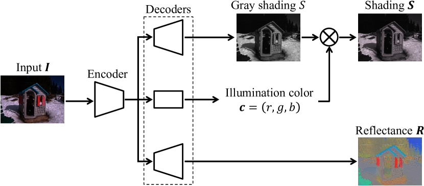
For the proposed method, we consider the color-illumination model in Eq. (2). Additionally, we assume that the illumination color of an image is the same for all pixels. As a result, shading is written as

$$\bm{S}(x,y) =S(x,y)\bm{c},$$ (3)

where $S(x,y)$ is shading in gray scale, and $\bm{c}$ is an RGB vector indicating the illumination color. Hence, the goal of the proposed method is to obtain reflectance $\bm{R}$, gray-shading $S$, and RGB vector $\bm{c}$ from given input image $\bm{I}$.

Figure 2 illustrates the architecture of the proposed network. Our network has a single encoder and three decoders. With the encoder, input image $\bm{I}$ is transformed into feature maps that are fed into decoders. An estimation $\hat{\bm{R}}$ of reflectance in RGB color space is directly obtained as an output of a reflectance decoder. In contrast, an estimation $\hat{\bm{S}}$ of shading is given as the product of estimated illumination color $\hat{\bm{c}}$ and estimated shading $\hat{S}$ in gray scale. $\hat{\bm{c}}$ and $\hat{S}$ are obtained by an illumination-color decoder and a shading decoder, respectively.

Figure 2: Proposed intrinsic image decomposition. Encoder maps given input image into features. Features are fed into three decoders: reflectance decoder, shading decoder, and illumination-color decoder. Reflectance/shading decoders produce reflectance/gray-shading components, respectively. Illumination-color decoder estimates illumination color. Colored shading can be obtained by multiplying gray-shading and illumination-color.

3.2 Loss functions

Let the $n$-th image set in the training dataset be $\{\bm{I}\}_{n}$ To fulfill all three premises in Section 2.2.2), our network is trained to minimize loss $\mathcal{L}$ calculated by using $\bm{I}_{1},\bm{I}_{2}\in\{\bm{I}\}_{n}$ as

$$\mathcal{L}=\mathbb{E}\left[\mathcal{L}_{\mathrm{reconst}}(\bm{I}_{1},\bm{I}_{2})+\mathcal{L}_{\mathrm{reflect}}(\bm{I}_{1},\bm{I}_{2})\right],$$ (4)

where $\mathcal{L}_{\mathrm{reconst}}$ and $\mathcal{L}_{\mathrm{reflect}}$ are loss functions for considering reconstruction and reflectance consistencies, respectively.

For the reconstruction consistency, in accordance with Eq. (2), we use $\mathcal{L}_{\mathrm{reconst}}$ given as

$$\mathcal{L}_{\mathrm{reconst}}(\bm{I}_{1},\bm{I}_{2}) =\lambda_{1}\left(\mathcal{L}_{\ell_{1}}(\bm{I}_{1},\hat{\bm{I}}_{1})+\mathcal{L}_{\ell_{1}}(\bm{I}_{2},\hat{\bm{I}}_{2})\right)$$

$$-\lambda_{2}\left(\mathcal{L}_{\cos}(\bm{I}_{1},\hat{\bm{I}}_{1})+\mathcal{L}_{\cos}(\bm{I}_{2},\hat{\bm{I}}_{2})\right),$$ (5)

where $\hat{\bm{I}}_{i},i\in\{1,2\}$ is an image reconstructed from estimated reflectance $\hat{\bm{R}}_{i}$, gray-scale shading $\hat{S}_{i}$, and illumination color $\hat{\bm{c}}_{i}$ for image $I_{i}$. From Eqs. (2) and (3), $\hat{\bm{I}}_{i}$ is calculated as

$$\hat{\bm{I}}_{i}(x,y)=\left(\hat{S}(x,y)\hat{\bm{c}}_{i}\right)\odot\hat{\bm{R}}_{i}(x,y).$$ (6)

$\mathcal{L}_{\ell_{1}}$ is the mean absolute error, and $\mathcal{L}_{\cos}$ is cosine similarity given by

$$\mathcal{L}_{\cos}(\bm{I},\hat{\bm{I}})=\frac{1}{|P|}\sum_{(x,y)\in P}\frac{\langle\bm{I}(x,y),\hat{\bm{I}}(x,y)\rangle}{\|\bm{I}(x,y)\|_{2}\cdot\|\hat{\bm{I}}(x,y)\|_{2}}.$$ (7)

For the reflectance consistencies, we designed $\mathcal{L}_{\mathrm{reflect}}$ as

$$\mathcal{L}_{\mathrm{reflect}}(\bm{I}_{1},\bm{I}_{2}) =\lambda_{3}\mathcal{L}_{\ell_{1}}(\hat{\bm{R}}_{1},\hat{\bm{R}}_{2})$$

$$+\lambda_{4}\left(\mathcal{L}_{\mathrm{lum}}(\hat{\bm{R}}_{1})+\mathcal{L}_{\mathrm{lum}}(\hat{\bm{R}}_{2})\right)$$

$$+\lambda_{5}\left(\mathcal{L}_{\ell_{1}}(\bm{c}_{1},\hat{\bm{c}}_{1})+\mathcal{L}_{\ell_{1}}(\bm{c}_{2},\hat{\bm{c}}_{2})\right),$$ (8)

$$\mathcal{L}_{\mathrm{lum}}(\bm{R}) =\frac{1}{|P|}\sum_{(x,y)\in P}\|0.5-\langle\bm{R}(x,y),\bm{v}\rangle\|_{1}$$ (9)

where vector $\bm{v}=(0.2126,0.7152,0.0722)^{\top}$ consists of coefficients for calculating the luminance of an RGB vector, and $\mathcal{L}_{\mathrm{lum}}$ is utilized for normalizing the luminance of reflectance to $0.5$. By normalizing the luminance to $0.5$, our network can output reflectance $\hat{\bm{R}}_{i}$ so that it is consistent regardless of the illumination-brightness conditions. Moreover, by minimizing $\ell_{1}$-distance between $\bm{c}_{i}$ and $\hat{\bm{c}}_{i}$, reflectance $\hat{\bm{R}}$ can also be consistent regardless of illumination-color conditions.

$\lambda_{1},\lambda_{2},\lambda_{3},\lambda_{4}$, and $\lambda_{5}$ are weights of the loss terms, In practice, we empirically set $\lambda_{1}=3,\lambda_{2}=1,\lambda_{3}=2,\lambda_{4}=1$, and $\lambda_{5}=1$ as weights.

3.3 Network architecture

The proposed network consists of an encoder, a reflectance decoder, a shading decoder, and an illuminant-color decoder. Figure 3 shows the network architecture of the encoder and reflectance/shading decoders in detail. The input image is an RGB color image of $H\times W$ pixels.

Figure 3: Network architecture of encoder and reflectance/shading decoders. Each box denotes multi-channel feature map produced by each layer. Number of channels is denoted above each box. Feature map resolutions are denoted to left of boxes.

For the encoder and the reflectance/shading decoders, we use four types of layers as shown in Fig. 3:

$3\times 3$ Conv. + BN + ReLU

,  which calculates a $3\times 3$ convolution with a stride of $1$ and a padding of $1$. After the convolution, batch normalization ioffe2015batch and the rectified linear unit activation function glorot2011deep (ReLU) are applied. Two adjacent $3\times 3$ Conv. + BN + ReLU layers will have the same number $K$ of filters, where $K$ (i.e., the number of channels) is denoted in Fig. 3.

$1\times 1$ Conv. + ReLU

,  which calculates a $1\times 1$ convolution with a stride of $1$ and without padding. After the convolution, ReLU is applied. The number of filters in the layer is $3$.

$3\times 3$ Conv. w/ stride $2$

,  which downsamples feature maps using a $3\times 3$ convolution with a stride of $2$ and a padding of $1$.

$4\times 4$ Transposed conv. w/ stride $1/2$

,  which upsamples feature maps using a $4\times 4$ transposed convolution with a stride of $1/2$ and a padding of $1$.

The proposed network has concatenated skip connections between the encoder and the decoders like U-Net ronneberger2015unet , Feature maps from intermediate layers in the encoder are concatenated with those from intermediate layers in the reflectance and shading decoders.

In addition to these three sub-networks, we utilize an illumination-color decoder that estimates the illumination color of a given image. The decoder consists of double $3\times 3$ Conv. + BN + ReLU layers, a global average pooling layer, and a $1\times 1$ conv. + ReLU layer. The $3\times 3$ Conv. + BN + ReLU layers all have $64$ filters, and the $1\times 1$ conv. + ReLU layer has $3$ filters. As a result, we can obtain a $3$-dimensional RGB vector that means the illumination color for each input image.

4 Training proposed network in self-supervised manner

To calculate the loss function for the proposed network, images of a single scene taken under various illumination-brightness and -color conditions are required. However, it is very costly to collect such images. For this reason, we generate pseudo images from raw images and use them for training the proposed network.

4.1 Simulating brightness change

A change in illumination brightness, i.e., radiance, affects image brightness. Here, we assume that camera parameters except for the shutter speed are fixed, although the image brightness can be controlled by adjusting various camera parameters. In this case, the image brightness is determined by the radiant power density at an imaging sensor, i.e., irradiance, and shutter speed, where the irradiance is proportional to the radiance.

Under the assumption that a scene is static during the time that the shutter is open and the sensor has a linear response with respect to the light intensity, the image brightness is proportional to the radiance (and also the shutter speed) kinoshita2019scene . Hence, the change in illumination brightness is simulated by multiplying an image $\bm{I}$ by a scalar value of $2^{v}$ as

$$\bm{I}^{\prime}(x,y)=2^{v}\bm{I}(x,y),$$ (10)

where it is equivalent to the exposure compensation of $v[\mathrm{EV}]$ kinoshita2019scene .

4.2 Simulating color change

The effect of illumination-color change is already considered in the research area of white balancing. White balancing aims to remove the effects of illumination color on an image. Typically, white balancing is performed by

$$\bm{I}^{\prime\prime}(x,y)=\mathrm{M}_{\mathrm{WB}}\bm{I}(x,y),$$ (11)

where

$$\mathrm{M}_{\mathrm{WB}}=\mathrm{M}_{A}^{-1}\begin{pmatrix}\alpha&0&0\\ 0&\beta&0\\ 0&0&\gamma\\ \end{pmatrix}\mathrm{M}_{A}$$ (12)

and $\mathrm{M}_{A}$ is a full-rank matrix with a size of $3\times 3$ for color space conversion. Parameters $\alpha,\beta$, and $\gamma$ are non-negative, and they are calculated from the ideal white illumination and illumination color $\bm{c}$ of an input image.

By using the inverse of $\mathrm{M}_{\mathrm{WB}}$, we can perform inverse white balancing as

$$\bm{I}(x,y)=\mathrm{M}_{\bm{c}}\bm{I}^{\prime\prime}(x,y),$$ (13)

where $\mathrm{M}_{\bm{c}}=\mathrm{M}_{\mathrm{WB}}^{-1}$. This corresponds to simulating illumination-color change.

For these reasons, illumination-brightness and -color changes can be simulated in accordance with Eqs. (10) and (11), respectively, by using various $v,\alpha,\beta$, and $\gamma$. Images generated by using the equations can be used for training the proposed network.

4.3 Procedure for data generation

In accordance with Eqs. (10) and (13), we randomly simulate images of a single scene taken under various illuminant-brightness and -color conditions, at every step of training. Images $\bm{I}_{i}$ are generated from a raw image $\bm{I}_{\mathrm{raw}}$ as follows.

1. Obtain an RGB image $\bm{I}$ by demosaicing and white-balancing a raw image $\bm{I}_{\mathrm{raw}}$.

2. Simulate illumination-color change in accordance with Eq.(10) as

   $$\bm{I}^{\prime}_{i}(x,y)=2^{v_{i}}\frac{0.18}{g(\bm{I})}\bm{I}(x,y),$$ (14)

   where $v_{i}$ is a uniform random number in the range of $[-1,1]$, and $g(\bm{I})$ indicates the geometric mean of the luminance of $\bm{I}$ reinhard2002photographic .

3. Simulate illumination-color change in accordance with Eq.(13) by multiplying $\bm{I}^{\prime}_{i}$ by $\mathrm{M}_{c_{i}}$ as

   $$\bm{I}_{i}(x,y)=\mathrm{M}_{c_{i}}\bm{I}^{\prime}_{i}(x,y),$$ (15)

   where $\mathrm{M}_{\bm{c}_{i}}$ is a diagonal matrix having $\bm{c}_{i}$ as the main diagonal, and $\bm{c}_{i}$ is a uniform random vector in $[0.9,1.1]^{3}$.

5 Simulation

We performed two simulation experiments to evaluate the proposed network in terms of the three consistencies, i.e., reconstruction consistency, reflectance consistency (brightness), and reflectance consistency (color).

5.1 Simulation using raw images

5.1.1 Experimental conditions

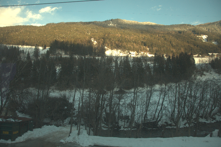
In this experiment, 45 image sets were generated from 45 raw images from the RAISE Dataset nguyen2015raise , where each image set consists of $9$ images. Figure 4 illustrates an example of an input image set. The generation procedure was the same as that in Section 4.4.3), where $v_{i}\in\{-1,0,+1\}$, and $\bm{c}_{i}\in\{(0.9,1.0,1.1),(1.0,1.0,1.0),(1.1,1.0,0.9)\}$. Each generated image $\bm{I}_{i}$ was independently fed into the trained network and decomposed into gray-shading $\hat{S}_{i}$, reflectance $\hat{\bm{R}}_{i}$, and illumination color $\hat{\bm{c}}_{i}$.

(a) $\bm{I}_{1}$

(b) $\bm{I}_{2}$

(c) $\bm{I}_{3}$

(d) $\bm{I}_{4}$

(e) $\bm{I}_{5}$

(f) $\bm{I}_{6}$

(g) $\bm{I}_{7}$

(h) $\bm{I}_{8}$

(i) $\bm{I}_{9}$

Figure 4: Example of input image set. Row denotes illumination brightness [Top: -1 EV, Middle: 0 EV, and Bottom: +1 EV], and column denotes illumination color [Left: Cold white (0.9, 1.0, 1.1), Middle: White (1.0, 1.0, 1.0), and Right: Warm white (1.1, 1.0, 0.9)]

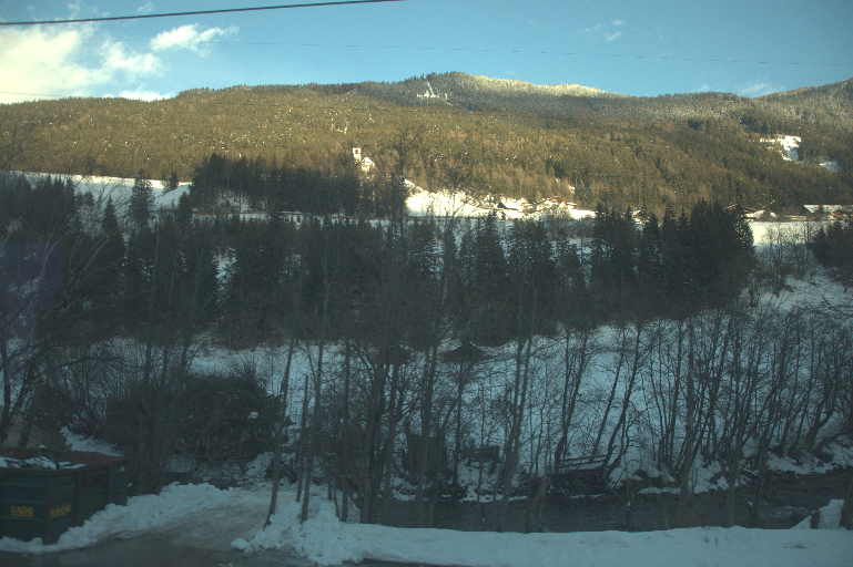
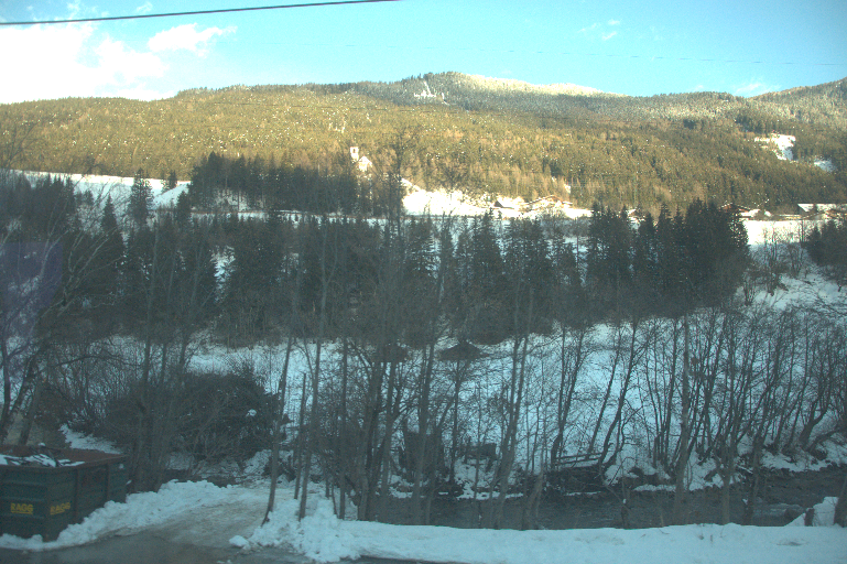
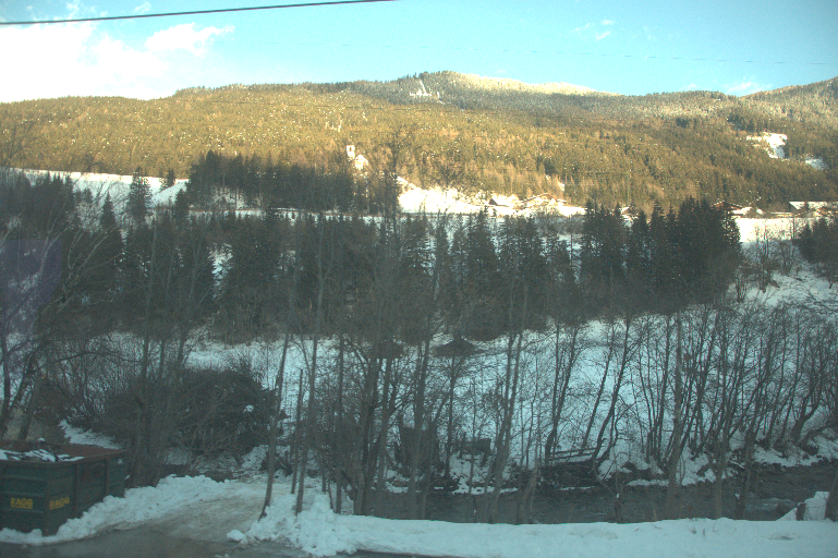
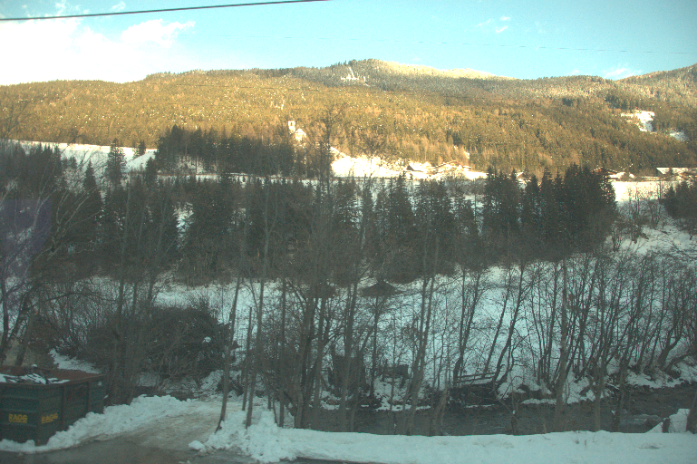
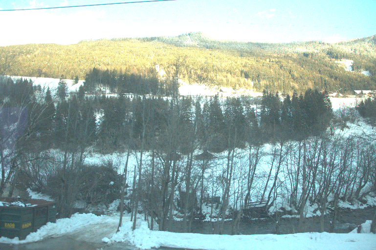
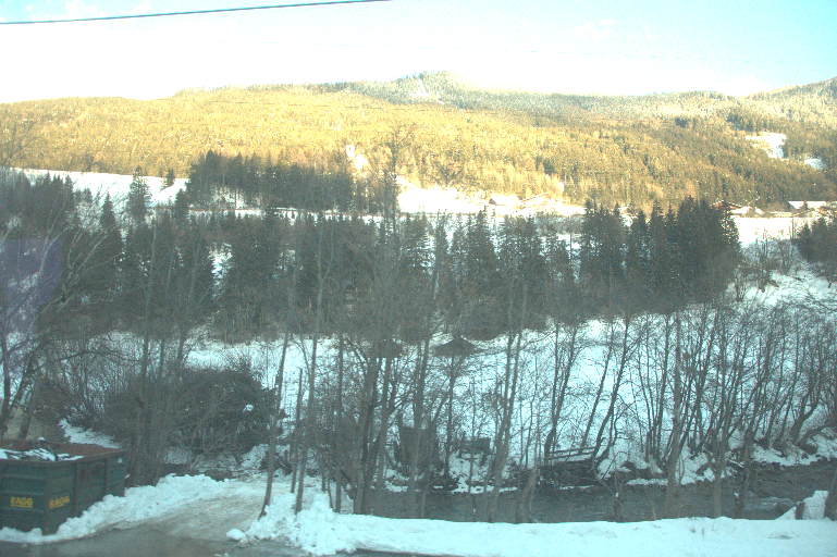
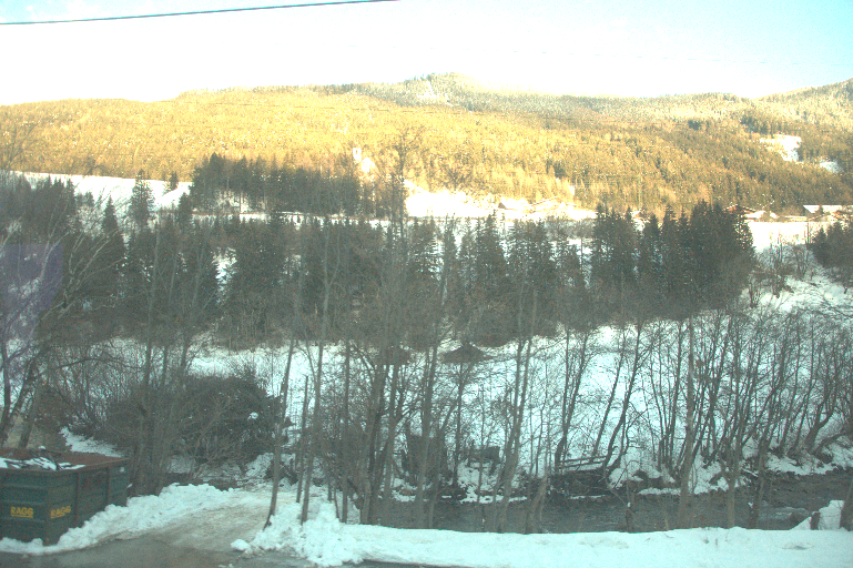
To evaluate the reconstruction consistency, we used the peak signal-to-noise ratio (PSNR), mean squared error (MSE), and structural dissimilarity (DSSIM) between input image $\bm{I}_{i}$ and reconstructed image $\hat{\bm{I}}_{i}$. Here, a larger PSNR value means higher similarity between two images. For MSE and DSSIM, a smaller value means higher similarity. To evaluate the reflectance consistency in terms of both brightness and color, we also used the PSNR, MSE, and DSSIM between a reference reflectance and an estimated reflectance $\hat{\bm{R}}_{i}$ of an image under another illumination condition. Here, $\hat{\bm{R}}_{5}$ was used as the reference reflectance.

The proposed network was compared with the following methods:

• Bell’s decomposition method bell2014intrinsic ,

• Unsupervised Learning for Intrinsic Image Decomposition from a Single Image (USI3D) liu2020unsupervised ,

where Bell’s method is an optimization based method and USI3D is a state-of-the-art DNN-based method. We used the authors’ original implementations of the two methods, which are available on GitHub.

Our network was trained with 100 epochs by using 3620 raw images from the HDR+ burst photography dataset hasinoff2016burst . For data augmentation, we resized each original input image with a random scaling factor in the range of $[0.6,1.0]$ for every epoch. After the resizing, we randomly cropped the resized image to an image patch with a size of $256\times 256$ pixels and flipped the patch horizontally with a probability of 0.5. In addition to the augmentation, we generated two images by applying the procedure in Section 4.4.3) to each augmented image in order to simulate various illumination-brightness and -color conditions. Loss was calculated by using the two generated images in accordance with Eq. (4) to Eq. (9). Here, the Adam optimizer kingma2014adam was utilized for optimization, where the parameters in Adam were set as $\alpha=0.001,\beta_{1}=0.9$, and $\beta_{2}=0.999$. He’s method he2015delving was used for initializing the network.

5.1.2 Experimental results

Figure 5 shows an example of decomposition with our network. From Fig. 5, we can see that the brightness of estimated reflectance $\hat{\bm{R}}$ was constant, and the estimated shading $\hat{\bm{S}}$ had a single color.

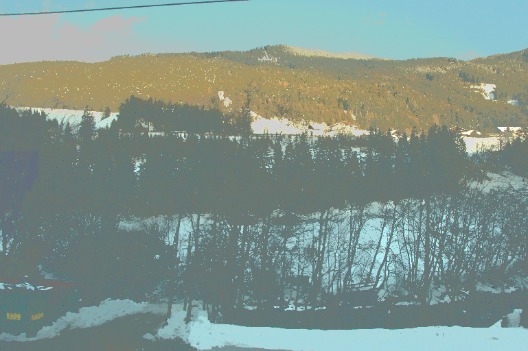
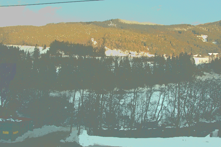
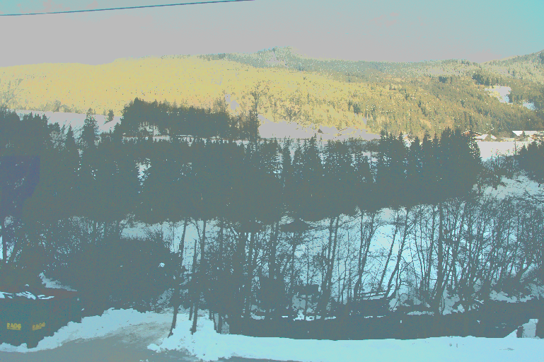
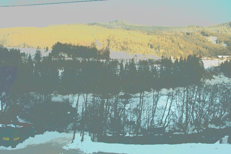
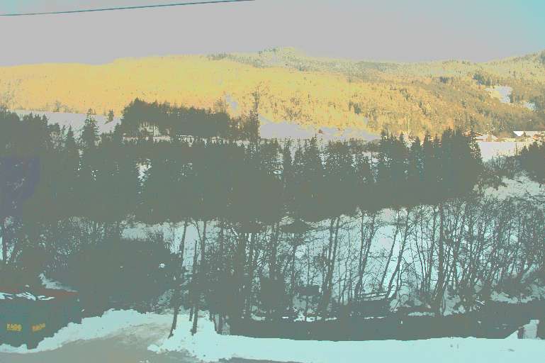
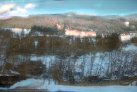
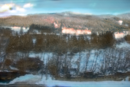
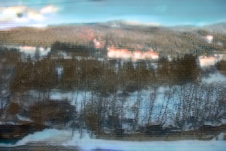
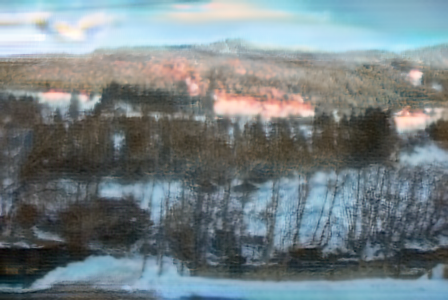
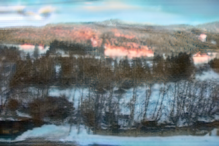
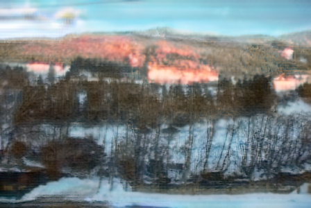
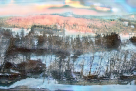
Figures 6, 7, and 8 are references of the images in Fig. 4 estimated by Bell’s method, USI3D, and the proposed network, respectively. From these figures, we can see that the estimated reflectance by the three methods is different. This is because the proposed network takes into account not only conventional reconstruction consistency but also two reflectance consistencies. The two reflectance consistencies require estimated reflectance to satisfy that it is independent from lighting conditions, i.e., brightness and illumination color. As shown in Figs 6 and 7, the conventional decomposition methods produced reflectance that depended on illumination brightness and color owing to the lack of consideration of reflectance consistencies. In contrast, the proposed network produced almost the same reflectance for all nine images that depended on illumination brightness and color. For this reason, the proposed network satisfied the reflectance consistencies in terms of brightness and color, but the conventional methods did not.

(a) Reflectance $\hat{\bm{R}}$

(b) Gray shading $\hat{S}$

(c) Shading $\hat{\bm{S}}$

Figure 5: Example of decomposition results by our network. Input image was $\bm{I}_{6}$ in Fig. 4.

(a) $\hat{\bm{R}}_{1}$

(b) $\hat{\bm{R}}_{2}$

(c) $\hat{\bm{R}}_{3}$

(d) $\hat{\bm{R}}_{4}$

(e) $\hat{\bm{R}}_{5}$

(f) $\hat{\bm{R}}_{6}$

(g) $\hat{\bm{R}}_{7}$

(h) $\hat{\bm{R}}_{8}$

(i) $\hat{\bm{R}}_{9}$

Figure 6: Example of estimated reflectance for images in Fig. 4 (Bell’s method bell2014intrinsic ). Row denotes illumination brightness [Top: -1 EV, Middle: 0 EV, and Bottom: +1 EV], and column denotes illumination color [Left: Cold white (0.9, 1.0, 1.1), Middle: White (1.0, 1.0, 1.0), and Right: Warm white (1.1, 1.0, 0.9)]

(a) $\hat{\bm{R}}_{1}$

(b) $\hat{\bm{R}}_{2}$

(c) $\hat{\bm{R}}_{3}$

(d) $\hat{\bm{R}}_{4}$

(e) $\hat{\bm{R}}_{5}$

(f) $\hat{\bm{R}}_{6}$

(g) $\hat{\bm{R}}_{7}$

(h) $\hat{\bm{R}}_{8}$

(i) $\hat{\bm{R}}_{9}$

Figure 7: Example of estimated reflectance for images in Fig. 4 (USI3D liu2020unsupervised ). Row denotes illumination brightness [Top: -1 EV, Middle: 0 EV, and Bottom: +1 EV], and column denotes illumination color [Left: Cold white (0.9, 1.0, 1.1), Middle: White (1.0, 1.0, 1.0), and Right: Warm white (1.1, 1.0, 0.9)]

(a) $\hat{\bm{R}}_{1}$

(b) $\hat{\bm{R}}_{2}$

(c) $\hat{\bm{R}}_{3}$

(d) $\hat{\bm{R}}_{4}$

(e) $\hat{\bm{R}}_{5}$

(f) $\hat{\bm{R}}_{6}$

(g) $\hat{\bm{R}}_{7}$

(h) $\hat{\bm{R}}_{8}$

(i) $\hat{\bm{R}}_{9}$

Figure 8: Example of estimated reflectance for images in Fig. 4 (Proposed). Row denotes illumination brightness [Top: -1 EV, Middle: 0 EV, and Bottom: +1 EV], and column denotes illumination color [Left: Cold white (0.9, 1.0, 1.1), Middle: White (1.0, 1.0, 1.0), and Right: Warm white (1.1, 1.0, 0.9)]

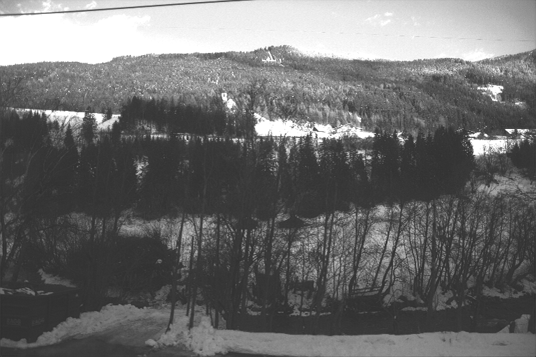
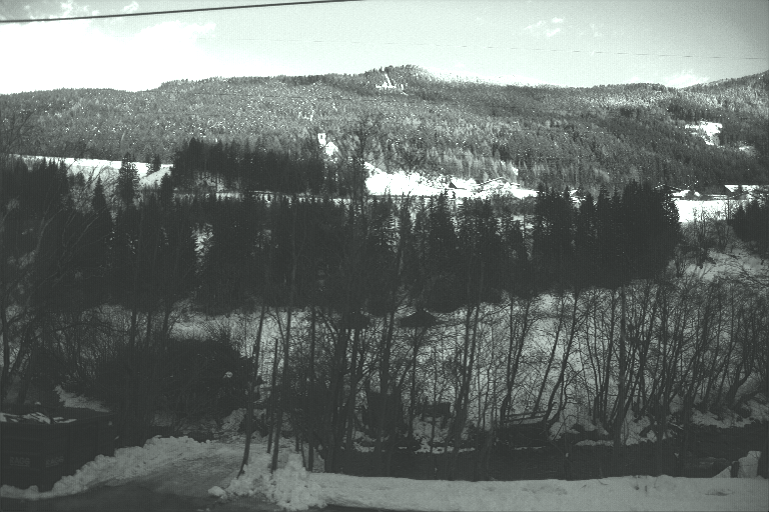
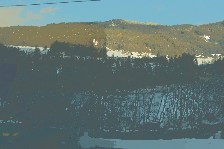
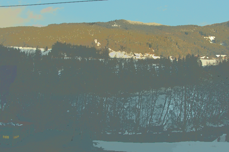
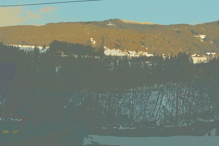
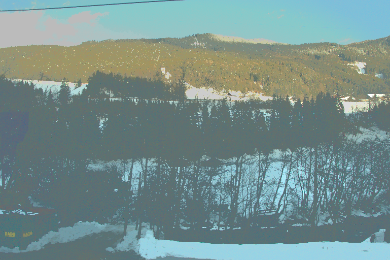
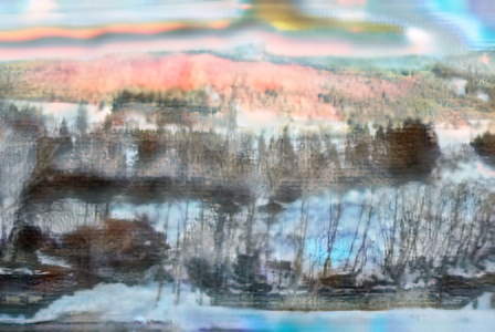
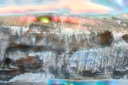
The reflectance consistencies of the proposed network were also confirmed in a numerical evaluation. Tables 2, 3, and 4 show the PSNR, MSE, and DSSIM values between $\hat{\bm{R}}_{i}$ and $\hat{\bm{R}}_{5}$ for each $i$ for the three methods, where these values were averaged over the 45 image sets that we used in this simulation. From Table 2, the proposed network provided higher PSNR values (about $30\mathrm{dB}$) than those of the conventional methods. Hence, the proposed network was shown to be robust against illumination-brightness/-color changes. This trend was also confirmed from Tables 3 and 4.

Table 2: PSNR values between $\hat{\bm{R}}_{i}$ and $\hat{\bm{R}}_{5}$ averaged over 45 image sets. Top: PSNR between $\hat{\bm{R}}_{1}$ and $\hat{\bm{R}}_{5}$, Bottom: PSNR between $\hat{\bm{R}}_{9}$ and $\hat{\bm{R}}_{5}$

	Bell bell2014intrinsic	USI3D liu2020unsupervised	Proposed
$\hat{\bm{R}}_{1}$ (-1 [EV], Cold white)	20.89	24.55	30.86
$\hat{\bm{R}}_{2}$ (-1 [EV], White)	21.62	25.10	31.00
$\hat{\bm{R}}_{3}$ (-1 [EV], Warm white)	20.77	24.65	30.09
$\hat{\bm{R}}_{4}$ (0 [EV], Cold white)	26.09	33.58	34.40
$\hat{\bm{R}}_{5}$ (0 [EV], White)	–	–	–
$\hat{\bm{R}}_{6}$ (0 [EV], Warm White)	26.75	32.97	34.56
$\hat{\bm{R}}_{7}$ (+1 [EV], Cold white)	18.22	18.90	28.84
$\hat{\bm{R}}_{8}$ (+1 [EV], White)	18.41	18.31	30.59
$\hat{\bm{R}}_{9}$ (+1 [EV], Warm white)	18.44	17.60	29.30

Table 3: MSE values between $\hat{\bm{R}}_{i}$ and $\hat{\bm{R}}_{5}$ averaged over 45 image sets. Top: MSE between $\hat{\bm{R}}_{1}$ and $\hat{\bm{R}}_{5}$, Bottom: MSE between $\hat{\bm{R}}_{9}$ and $\hat{\bm{R}}_{5}$

	Bell bell2014intrinsic	USI3D liu2020unsupervised	Proposed
$\hat{\bm{R}}_{1}$ (-1 [EV], Cold white)	0.013	0.007	0.001
$\hat{\bm{R}}_{2}$ (-1 [EV], White)	0.010	0.007	0.001
$\hat{\bm{R}}_{3}$ (-1 [EV], Warm white)	0.011	0.007	0.001
$\hat{\bm{R}}_{4}$ (0 [EV], Cold white)	0.004	0.001	0.000
$\hat{\bm{R}}_{5}$ (0 [EV], White)	0.000	0.000	0.000
$\hat{\bm{R}}_{6}$ (0 [EV], Warm white)	0.003	0.001	0.000
$\hat{\bm{R}}_{7}$ (1 [EV], Cold white)	0.016	0.015	0.001
$\hat{\bm{R}}_{8}$ (1 [EV], White)	0.017	0.018	0.001
$\hat{\bm{R}}_{9}$ (1 [EV], Warm white)	0.017	0.020	0.001

Table 4: DSSIM values between $\hat{\bm{R}}_{i}$ and $\hat{\bm{R}}_{5}$ averaged over 45 image sets. Top: DSSIM between $\hat{\bm{R}}_{1}$ and $\hat{\bm{R}}_{5}$, Bottom: DSSIM between $\hat{\bm{R}}_{9}$ and $\hat{\bm{R}}_{5}$

	Bell bell2014intrinsic	USI3D liu2020unsupervised	Proposed
$\hat{\bm{R}}_{1}$ (-1 [EV], Cold white)	0.073	0.031	0.016
$\hat{\bm{R}}_{2}$ (-1 [EV], White)	0.072	0.029	0.016
$\hat{\bm{R}}_{3}$ (-1 [EV], Warm white)	0.076	0.030	0.016
$\hat{\bm{R}}_{4}$ (0 [EV], Cold white)	0.029	0.008	0.004
$\hat{\bm{R}}_{5}$ (0 [EV], White)	0.000	0.000	0.000
$\hat{\bm{R}}_{6}$ (0 [EV], Warm white)	0.028	0.007	0.004
$\hat{\bm{R}}_{7}$ (1 [EV], Cold white)	0.098	0.057	0.024
$\hat{\bm{R}}_{8}$ (1 [EV], White)	0.099	0.061	0.023
$\hat{\bm{R}}_{9}$ (1 [EV], Warm white)	0.101	0.068	0.026

Tables 5, 6, and 7 show the PSNR, MSE, and DSSIM values between original image $\bm{I}_{i}$ and reconstructed image $\hat{\bm{I}}_{i}$ for each $i$ for the three methods, where these values were averaged over the 45 image sets that we used in this simulation. From Table 5, we confirmed that the proposed network outperformed USI3D in terms of the reconstruction consistency although Bell’s method provided the highest PSNR. This result indicates that current DNN-based methods such as USI3D have a limited performance in terms of reconstruction consistency compared with traditional optimization-based methods such as Bell’s method. The proposed network partially overcomes this limited performance of DNN-based methods. This trend was also confirmed from Tables 6 and 7.

Table 5: PSNR values between $\bm{I}_{i}$ and $\hat{\bm{I}}_{i}$ averaged over 45 image sets. Top: PSNR between $\bm{I}_{1}$ and $\hat{\bm{I}_{1}}$, Bottom: PSNR between $\bm{I}_{9}$ and $\hat{\bm{I}_{9}}$

	Bell bell2014intrinsic	USI3D liu2020unsupervised	Proposed
$\hat{\bm{I}}_{1}$ (-1 [EV], Cold white)	46.53	20.43	21.75
$\hat{\bm{I}}_{2}$ (-1 [EV], White)	46.47	20.64	21.81
$\hat{\bm{I}}_{3}$ (-1 [EV], Warm white)	46.55	20.66	21.78
$\hat{\bm{I}}_{4}$ (0 [EV], Cold white)	46.50	16.82	20.27
$\hat{\bm{I}}_{5}$ (0 [EV], White)	46.25	17.08	20.36
$\hat{\bm{I}}_{6}$ (0 [EV], Warm White)	46.19	17.14	20.37
$\hat{\bm{I}}_{7}$ (+1 [EV], Cold white)	45.47	14.72	20.34
$\hat{\bm{I}}_{8}$ (+1 [EV], White)	45.38	14.76	20.40
$\hat{\bm{I}}_{9}$ (+1 [EV], Warm white)	45.47	14.64	20.41

Table 6: MSE values between $\bm{I}_{i}$ and $\hat{\bm{I}}_{i}$ averaged over 45 image sets. Top: MSE between $\bm{I}_{1}$ and $\hat{\bm{I}_{1}}$, Bottom: MSE between $\bm{I}_{9}$ and $\hat{\bm{I}_{9}}$

	Bell bell2014intrinsic	USI3D liu2020unsupervised	Proposed
$\hat{\bm{I}}_{1}$ (-1 [EV], Cold white)	0.000	0.014	0.008
$\hat{\bm{I}}_{2}$ (-1 [EV], White)	0.000	0.014	0.008
$\hat{\bm{I}}_{3}$ (-1 [EV], Warm white)	0.000	0.014	0.008
$\hat{\bm{I}}_{4}$ (0 [EV], Cold white)	0.000	0.023	0.009
$\hat{\bm{I}}_{5}$ (0 [EV], White)	0.000	0.022	0.009
$\hat{\bm{I}}_{6}$ (0 [EV], Warm white)	0.000	0.022	0.009
$\hat{\bm{I}}_{7}$ (1 [EV], Cold white)	0.000	0.036	0.008
$\hat{\bm{I}}_{8}$ (1 [EV], White)	0.000	0.036	0.008
$\hat{\bm{I}}_{9}$ (1 [EV], Warm white)	0.000	0.037	0.008

Table 7: DSSIM values between $\bm{I}_{i}$ and $\hat{\bm{I}}_{i}$ averaged over 45 image sets. Top: DSSIM between $\bm{I}_{1}$ and $\hat{\bm{I}_{1}}$, Bottom: DSSIM between $\bm{I}_{9}$ and $\hat{\bm{I}_{9}}$

	Bell bell2014intrinsic	USI3D liu2020unsupervised	Proposed
$\hat{\bm{I}}_{1}$ (-1 [EV], Cold white)	0.001	0.161	0.121
$\hat{\bm{I}}_{2}$ (-1 [EV], White)	0.001	0.162	0.122
$\hat{\bm{I}}_{3}$ (-1 [EV], Warm white)	0.001	0.165	0.124
$\hat{\bm{I}}_{4}$ (0 [EV], Cold white)	0.001	0.204	0.101
$\hat{\bm{I}}_{5}$ (0 [EV], White)	0.001	0.204	0.102
$\hat{\bm{I}}_{6}$ (0 [EV], Warm white)	0.001	0.206	0.103
$\hat{\bm{I}}_{7}$ (1 [EV], Cold white)	0.001	0.239	0.085
$\hat{\bm{I}}_{8}$ (1 [EV], White)	0.001	0.240	0.086
$\hat{\bm{I}}_{9}$ (1 [EV], Warm white)	0.001	0.242	0.087

5.2 Simulation using MIT intrinsic images dataset

5.2.1 Experimental conditions

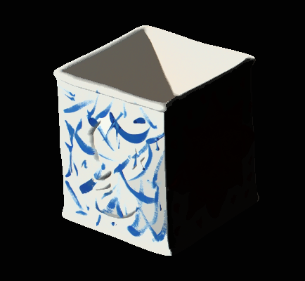
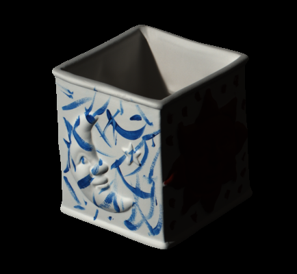
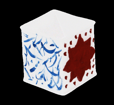
To further study features of the proposed network, we conducted simulation experiments using the MIT intrinsic images dataset grosse2009groundtruth , which is a typical dataset for intrinsic image decomposition. An example of an image “box” in the dataset is shown in Fig. 9. The MIT intrinsic images dataset provides not only original images but also the corresponding groundtruth reflectance and shading for each image. For constructing the dataset, computer graphics techniques were utilized.

(a) Original image

(b) Reflectance

(c) Shading

Figure 9: Groundtruth image “box” in Mit intrinsic image dataset grosse2009groundtruth

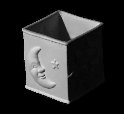
Because groundtruth reflectance and shading components are available for each image, in this experiment, we used the local mean squared error (LMSE) score grosse2009groundtruth to evaluate the performance of the proposed network. Here, a smaller LMSE score value means higher similarity between an estimation and the corresponding groundtruth.

Other conditions were the same as those in Section 5.5.1

5.2.2 Expeirmental results

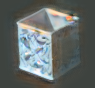
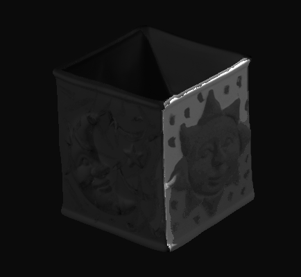
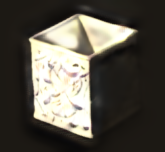
Figures 10 and 11 show estimated reflectance and shading components, respectively, for an image “box” in MIT intrinsic images dataset estimated by Bell’s method, USI3D, and the proposed network. As shown in Fig. 10, the reflectance component estimated by the proposed network was significantly different from the groundtruth one shown in Fig. 9. This is because the proposed network was trained with luminance normalization of the reflectance in Eq. (9). When there are no constraints on the luminance of reflectance, intrinsic image decomposition suffers from scale indeterminacy. In this case, when an image $\bm{I}$ is decomposed as $\bm{I}(x,y)=\bm{S}(x,y)\odot\bm{R}(x,y)$ there is another solution $\bm{I}(x,y)=(a\bm{S}(x,y))\odot(a^{-1}\bm{R}(x,y))$, where $a>0$. This scale indeterminacy may be solved by supervised learning using a large high-quality dataset. However, it is difficult to prepare the ground truth of reflectance and shading in real scenes. For this reason, we aim at intrinsic image decomposition by unsupervised learning, and the proposed network was trained with the luminance normalization to remove the scale indeterminacy. By using the normalization, the proposed network estimated shading components more accurately than the conventional methods, as shown in Fig. 11. This is also confirmed by the fact that the proposed network provided LMSE scores as well as the conventional methods, as in Table 8.

(a) Bell bell2014intrinsic

(b) USI3D liu2020unsupervised

(c) Proposed

Figure 10: Estimated reflectance for image “box” in Mit intrinsic image dataset

(a) Bell bell2014intrinsic

(b) USI3D liu2020unsupervised

(c) Proposed

Figure 11: Estimated shading for image “box” in Mit intrinsic image dataset

Table 8: LMSE scores for 16 images in MIT intrinsic dataset

	Bell bell2014intrinsic	USI3D liu2020unsupervised	Proposed
Box	0.210	0.056	0.067
Cup1	0.088	0.045	0.052
Cup2	0.130	0.062	0.085
Deer	0.173	0.091	0.109
Dinosaur	0.133	0.072	0.095
Frog1	0.215	0.053	0.075
Frog2	0.269	0.114	0.059
Panther	0.098	0.045	0.062
Paper1	0.051	0.026	0.025
Paper2	0.048	0.030	0.032
Raccoon	0.143	0.049	0.040
Squirrel	0.208	0.061	0.071
Sun	0.064	0.042	0.052
Teabag1	0.098	0.179	0.197
Teabag2	0.092	0.129	0.161
Turtle	0.166	0.078	0.052
Mean (16 images)	0.137	0.071	0.077

6 Conclusion

In this paper, we proposed a novel intrinsic image decomposition network considering reflectance consistency. In the proposed network, reconstruction consistency, reflectance consistency (brightness), and reflectance consistency (color) are considered by using a color-illuminant model and training the network with losses calculated from images taken under various illumination conditions. In addition, the proposed network can be trained in a self-supervised manner because various illumination conditions can easily be simulated. Experimental results show that our network can decompose images into reflectance and shading components while maintaining the reflectance consistencies in terms of both illumination-brightness and -colors.

Since the proposed network can produce robust reflectance against changes of illumination conditions, the proposed network will contribute to varous color image processing such as image enhancement while preserving object color and more realistic white balance adjustment.

Financial Support

“None.”

Statement of interest

“None.”

Biographies

Yuma Kinoshita received his B.Eng., M.Eng., and the Ph.D. degrees from Tokyo Metropolitan University, Japan, in 2016, 2018, and 2020 respectively. Since April 2020, he has been a project assistant professor at Tokyo Metropolitan University. His research interests are in the area of signal processing, image processing, and machine learning. He is a Member of IEEE, APSIPA, IEICE, and ASJ. He received the IEEE ISPACS Best Paper Award, in 2016, the IEEE Signal Processing Society Japan Student Conference Paper Award, in 2018, the IEEE Signal Processing Society Tokyo Joint Chapter Student Award, in 2018, the IEEE GCCE Excellent Paper Award (Gold Prize), in 2019, and the IWAIT Best Paper Award, in 2020. He was a Registration Chair of DCASE2020 Workshop.

Hitoshi Kiya received his B.E. and M.E. degrees from the Nagaoka University of Technology, Japan, in 1980 and 1982, respectively, and his Dr.Eng. degree from Tokyo Metropolitan University in 1987. In 1982, he joined Tokyo Metropolitan University, where he became a Full Professor in 2000. From 1995 to 1996, he attended The University of Sydney, Australia, as a Visiting Fellow. He is a fellow of IEEE, IEICE, and ITE. He was a recipient of numerous awards, including 10 best paper awards. He served as the President of APSIPA from 2019 to 2020, and the Regional Director-at-Large for Region 10 of the IEEE Signal Processing Society from 2016 to 2017. He was also the President of the IEICE Engineering Sciences Society from 2011 to 2012. He has been an editorial board member of eight journals, including IEEE Transactions on Signal Processing, IEEE Transactions on Image Processing, and IEEE Transactions on Information Forensics and Security, and a member of nine technical committees, including the APSIPA Image, Video, and Multimedia Technical Committee (TC), and IEEE Information Forensics and Security TC. He has organized a lot of international conferences in such roles as the TPC Chair of IEEE ICASSP 2012 and as the General Co-Chair of IEEE ISCAS 2019.

References

- (1) X. Fu, D. Zeng, Y. Huang, X.-P. Zhang, and X. Ding, “A Weighted Variational Model for Simultaneous Reflectance and Illumination Estimation,” in Proceedings of IEEE Conference on Computer Vision and Pattern Recognition, Jun. 2016, pp. 2782–2790.
- (2) X. Guo, Y. Li, and H. Ling, “LIME: Low-Light Image Enhancement via Illumination Map Estimation,” IEEE Transactions on Image Processing, vol. 26, no. 2, pp. 982–993, Feb. 2017.
- (3) C.-C. Chien, Y. Kinoshita, S. Shiota, and H. Kiya, “A Retinex-based image enhancement scheme with noise aware shadow-up function,” in Proceedings of International Workshop on Advanced Image Technology, Mar. 2019, paper no. 110492K.
- (4) H. G. Barrow and J. M. Tenenbaum, “Recovering intrinsic scene characteristics from images,” AI Center, SRI International, Tech. Rep., 1978.
- (5) R. Grosse, M. K. Johnson, E. H. Adelson, and W. T. Freeman, “Ground-truth dataset and baseline evaluations for intrinsic image algorithms,” Proceedings of International Conference on Computer Vision, 2009.
- (6) E. H. Land, “The retinex theory of color vision,” Scientific american, vol. 237, no. 6, pp. 108–129, 1977.
- (7) Y. Weiss, “Deriving intrinsic images from image sequences,” in Proceedings of IEEE International Conference on Computer Vision, 2001, pp. 68–75.
- (8) S. Bell, K. Bala, and N. Snavely, “Intrinsic images in the wild,” ACM Transactions on Graphics, vol. 33, no. 4, pp. 1–12, Jul. 2014.
- (9) T. Zhou, P. Kr"ahenb"uhl, and A. A. Efros, “Learning data-driven reflectance priors for intrinsic image decomposition,” in Proceedings of IEEE International Conference on Computer Vision, 2015, pp. 3469–3477.
- (10) W.-C. Ma, H. Chu, B. Zhou, R. Urtasun, and A. Torralba, “Single Image Intrinsic Decomposition Without a Single Intrinsic Image,” in Proceedings of European Conference on Computer Vision, 2018, pp. 211–229.
- (11) Q. Fan, J. Yang, G. Hua, B. Chen, and D. Wipf, “Revisiting Deep Intrinsic Image Decompositions,” in IEEE/CVF Conference on Computer Vision and Pattern Recognition, Jun. 2018, pp. 8944–8952.
- (12) Z. Li and N. Snavely, “CGIntrinsics: Better Intrinsic Image Decomposition through Physically-Based Rendering,” Proceedings of European Conference on Computer Vision, Aug. 2018.
- (13) ——, “Learning Intrinsic Image Decomposition from Watching the World,” in Proceedings of IEEE Conference on Computer Vision and Pattern Recognition, Jun. 2018, pp. 9039–9048.
- (14) L. Lettry, K. Vanhoey, and L. Van Gool, “Unsupervised Deep Single-Image Intrinsic Decomposition using Illumination-Varying Image Sequences,” Computer Graphics Forum, vol. 37, no. 7, pp. 409–419, Oct. 2018.
- (15) Z. Wang and F. Lu, “Single Image Intrinsic Decomposition with Discriminative Feature Encoding,” in Proceedings of IEEE/CVF International Conference on Computer Vision Workshop, Oct. 2019, pp. 4310–4319.
- (16) Y. Liu, Y. Li, S. You, and F. Lu, “Unsupervised Learning for Intrinsic Image Decomposition from a Single Image,” in Proceedings of IEEE Conference on Computer Vision and Pattern Recognition, Jun. 2020, pp. 3245–3254.
- (17) L. Shen and C. Yeo, “Intrinsic images decomposition using a local and global sparse representation of reflectance,” in Proceedings of IEEE Conference on Computer Vision and Pattern Recognition, Jun. 2011, pp. 697–704.
- (18) J. Chang, R. Cabezas, and J. W. Fisher, “Bayesian Nonparametric Intrinsic Image Decomposition,” in Proceedings of European Conference on Computer Vision, Sep. 2014, pp. 704–719.
- (19) D. J. Butler, J. Wulff, G. B. Stanley, and M. J. Black, “A Naturalistic Open Source Movie for Optical Flow Evaluation,” in Proceedings of European Conference on Computer Vision, 2012, pp. 611–625.
- (20) S. Ioffe and C. Szegedy, “Batch Normalization: Accelerating Deep Network Training by Reducing Internal Covariate Shift,” arXiv preprint arXiv:1502.03167, pp. 1–11, Feb. 2015. [Online]. Available: http://arxiv.org/abs/1502.03167
- (21) X. Glorot, A. Bordes, and Y. Bengio, “Deep sparse rectifier neural networks,” in Proceedings of the International Conference on Artificial Intelligence and Statistics, Apr. 2011, pp. 315–323.
- (22) O. Ronneberger, P.Fischer, and T. Brox, “U-Net: Convolutional Networks for Biomedical Image Segmentation,” in Medical Image Computing and Computer-Assisted Intervention (MICCAI), ser. LNCS, vol. 9351, Springer, Nov. 2015, pp. 234–241.
- (23) Y. Kinoshita and H. Kiya, “Scene Segmentation-Based Luminance Adjustment for Multi-Exposure Image Fusion,” IEEE Transactions on Image Processing, vol. 28, no. 8, pp. 4101–4116, Aug. 2019.
- (24) E. Reinhard, M. Stark, P. Shirley, and J. Ferwerda, “Photographic tone reproduction for digital images,” ACM Transactions on Graphics, vol. 21, no. 3, pp. 267–276, Jul. 2002.
- (25) D.-T. Dang-Nguyen, C. Pasquini, V. Conotter, and G. Boato, “RAISE - A Raw Images Dataset for Digital Image Forensics,” in Proceedings of ACM Multimedia Systems Conference, Mar. 2015, pp. 219–224.
- (26) S. W. Hasinoff, D. Sharlet, R. Geiss, A. Adams, J. T. Barron, F. Kainz, J. Chen, and M. Levoy, “Burst photography for high dynamic range and low-light imaging on mobile cameras,” ACM Transactions on Graphics, vol. 35, no. 6, pp. 1–12, Nov. 2016.
- (27) D. P. Kingma and J. Ba, “Adam: A Method for Stochastic Optimization,” arXiv preprint arXiv:1412.6980, pp. 1–15, Dec. 2014. [Online]. Available: http://arxiv.org/abs/1412.6980
- (28) K. He, X. Zhang, S. Ren, and J. Sun, “Delving Deep into Rectifiers: Surpassing Human-Level Performance on ImageNet Classification,” in Proceedings of IEEE International Conference on Computer Vision, Dec. 2015, pp. 1026–1034.