Performance Analysis under IRS-User Association for Distributed IRSs Assisted MISO Systems

Abstract

Distributed intelligent reflecting surfaces (IRSs) deployed in multi-user wireless communication systems promise improved system performance. However, the signal-to-interference-plus-noise ratio (SINR) analysis and IRSs optimization in such a system become challenging, due to the large number of involved parameters. The system optimization can be simplified if users are associated with IRSs, which in turn focus on serving the associated users. We provide a practical theoretical framework for the average SINR analysis of a distributed IRSs-assisted multi-user MISO system, where IRSs are optimized to serve their associated users. In particular, we derive the average SINR expression under maximum ratio transmission (MRT) precoding at the BS and optimized reflect beamforming configurations at the IRSs. A successive refinement (SR) method is then outlined to optimize the IRS-user association parameters for the formulated max-min SINR problem which motivates user-fairness. Simulations validate the average SINR analysis while confirming the superiority of a distributed IRSs system over a centralized IRS system as well as the gains with optimized IRS-user association as compared to random association.

I Introduction

With the imminence of massive connectivity promising a plethora of devices to be able to communicate effectively comes a new set of problems. How to create robust, high-speed links sustained over a wide range of geographical locations for many devices? Smart radio environments, where the environment is jointly optimized along with the transmitter and receiver, is a promising concept to solve these problems [1]. To enable the control of radio environments, communication engineers are exploring the idea of deploying software-controlled surfaces, referred to as intelligent reflecting surfaces (IRSs), on structures in the environment such as buildings. Each IRS contains a large number of low-cost, passive reflecting elements, where each element can introduce a phase shift onto the impinging electromagnetic (EM) waves to achieve a desired objective. This objective can be in the form of increasing the received power of the desired signal at a receiver, or decreasing the power of interference, or increasing the ratio between the two. An IRS can help to achieve these objectives via beam-focusing, which is tuning the magnitude of the radiation pattern in a certain direction, and/or beam-steering which is modifying the direction of the beam.

Designing IRS phase shifts to shape the impinging EM waves, referred to as passive (or reflect) beamforming, has been studied extensively in recent literature [2, 3, 4, 5]. The works in [2], [3], and [5] focus on jointly optimizing transmit beamforming at the BS and passive beamforming at the IRS to meet a certain goal such as maximizing energy efficiency [5], maximizing minimum user SINR subject to a transmit power constraint [2], or minimizing transmit power subject to quality of service constraints [3]. IRSs have also been studied to enhance physical layer security in [6]. For a general setting with frequency selective channels, an IRS-aided orthogonal frequency division multiplexing (OFDM) based wireless system is tackled in [7] and [8]. Moreover, IRSs have found applications in simultaneous wireless information and power transfer (SWIPT) [9], [10]. All these works consider a single IRS in their system model.

The current literature on distributed IRSs focus on the design of reflect beamforming to increase coverage and performance [11, 12]. The authors in [11] study the effects of large-scale deployment of IRSs in cellular communication by equipping blocking structures with IRSs and eliminating blind-spots. Generally, deploying a single IRS in the line of sight (LoS) of the BS can reduce the degrees of freedom of the overall channel to one (or a low number as compared to the number of BS antennas and IRS elements) [13]. The resulting rank deficient system can not serve multiple users simultaneously. In [12], distributed IRSs are explored as a promising solution to the rank-deficiency problem because the overall BS-IRS channel in the distributed IRSs case would be the sum of multiple rank one channels which guarantees higher rank channels. The goal in [12] is to maximize sum-rate via jointly optimizing the transmit power and the phase shift matrices at all the distributed IRSs. The authors in [14] handle the IRS-user association problem by assigning IRSs to users to optimally balance the passive beamforming gains among different BS-user links. Moreover, they derive the signal-to-interference-plus-noise ratio (SINR) expression at each user in closed form, and create an SINR balancing optimization problem to find the IRS-user association parameters. However, their system model assumes single-antenna BSs to simplify the analysis.

In this work, we formulate and solve a max-min average SINR optimization problem for a distributed IRSs assisted multi-user MISO system to find the optimal IRS-user association. We focus on the average (ergodic) analysis of the SINR at each user, under the scenario where each IRS is associated with one user in the system. For a particular IRS-user association pair, we choose the design for IRS phase shifts that would maximize the received signal strength at that user. Under that design, we utilize statistical tools to obtain a closed form expression for the average SINR at each user. Finally, we outline a low-complexity SR algorithm to find the IRS-user association parameters that maximize the minimum SINR subject to constraints on the values of binary association parameters. The optimization of IRS-user association in a distributed IRSs setting has been rarely dealt with in literature, and as more research expands in IRS-aided systems, a natural outcome is to have IRSs deployed in different geographical locations associated with different users or groups of users, in order to sustain and enable the concept of smart radio environments. In particular, the existing work on IRS-user association [14] simplifies the system model by assuming single-antenna BSs, while in our work we consider a multiple-antenna BS which is practical.

The results illustrate the significance of associating the IRSs with users in an optimized fashion resulting in an increase in the SINR of the bottleneck user, when compared to settings where the IRSs are randomly assigned to the users or where the IRSs are assigned based on the minimum distance to the users. The results also showcase the close performance of SR algorithm to the optimal but computationally expensive exhaustive search in finding the association parameters. The performance improvement by distributing the IRSs in different geographical locations instead of having a centralized IRS unit is also illustrated.

This paper is organized as follows. Sec. II introduces the distributed IRSs assisted multi-user MISO system model. Sec. III performs the ergodic SINR analysis for all users and Sec. IV solves the IRS-user association problem with max-min average SINR as an objective. Numerical evaluations and discussions on performance are provided in Sec. V. Finally, Sec. VI concludes the paper and highlights future directions.

Notation: This notation is used throughout the work. Bold lower-case and upper-case characters denote vectors and matrices, respectively. The subscripts $(\cdot)^{T}$ and $(\cdot)^{H}$ represent the transpose and Hermitian, respectively. The operator $tr(\cdot)$ is the trace of matrix, while the $\mathbb{E}[\cdot]$ and $\text{Var}[\cdot]$ are the expectation and variance of a random variable, respectively. The Kronecker and Hadamard products are denoted as $\otimes$ and $\odot$, respectively. For a complex number $x$, define its conjugate as $x^{*}$, $|x|$ as its magnitude, $\angle x$ as its phase (for vectors, the magnitude and phase are taken element-wise). The Euclidean norm of a vector is defined as $\|\cdot\|$. For a diagonal matrix $\mathbf{D}$, $\text{diag}(\mathbf{D})$ refers to its vectored form, while for a a vector $\mathbf{v}$, $\text{diag}(\mathbf{v})$ creates a diagonal matrix. An $M\times M$ identity matrix is denoted by $\mathbf{I}_{M}$, moreover $\mathbf{1}_{M}$ defines an $M\times M$ all-ones matrix.

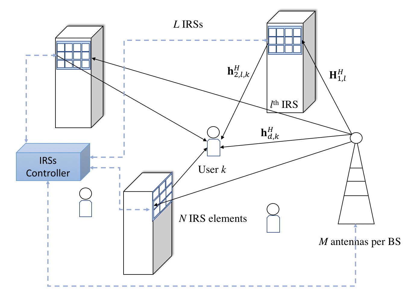
Figure 1: Distributed IRSs assisted MISO system model.

II System Model

Consider an $M$-antenna BS serving $K$ single-antenna users in the downlink, while being assisted by $L$ IRSs each equipped with $N$ elements (see Fig. 1). The IRSs are deployed in the environment in a distributed manner with fixed positions, and their operation is controlled by a centralized IRS controller that communicates with the BS over a backhaul link [2].

The channels are modeled as Rayleigh fading for the direct BS-user and IRS-user links, and as LoS for each BS-IRS link. We assume that the BS has perfect channel state information (CSI) to design the precoder and IRS reflect beamforming vectors. While perfect CSI acquisition is challenging in IRS-assisted systems, we make this assumption to enable a tractable theoretical analysis of the distributed IRSs assisted system, which is already complex given the large number of links involved.

II-A Downlink Transmission

The overall channel between the BS and user $k$ is given by

$$\mathbf{h}_{k}=\mathbf{h}_{d,k}+\sum_{l=1}^{L}\mathbf{H}_{1,l}\boldsymbol{\Theta}_{l}\mathbf{h}_{2,l,k},$$ (1)

where $\mathbf{h}_{d,k}\in\mathbb{C}^{M\times 1}$ is the direct channel between BS and user $k$, $\mathbf{H}_{1,l}\in\mathbb{C}^{M\times N}$ is the channel between BS and IRS $l$, $\mathbf{h}_{2,l,k}\in\mathbb{C}^{N\times 1}$ is the channel between IRS $l$ and user $k$, and $\boldsymbol{\Theta}_{l}=\text{diag}(\alpha_{l,1}e^{j\theta_{l,1}},\dots,$ $\alpha_{l,N}e^{j\theta_{l,N}})\in\mathbb{C}^{N\times N}$ is the reflection matrix for IRS $l$, where $\theta_{l,n}\in[0,2\pi]$ is the phase-shift applied by element $n$ of IRS $l$ and $\alpha_{l,n}\in[0,1]$ is the amplitude reflection coefficient. We assume the reflection coefficients $\alpha_{l,n}$’s to equal one, as done in most current works on IRSs motivated by the significant advancements made in the design of lossless metasurfaces [15]. The analysis can be straightforwardly extended to arbitrary values of $\alpha_{l,n}$s.

The received baseband signal in the downlink at user $k$ is defined as

$${y}_{k}=\mathbf{h}_{k}^{H}\mathbf{x}+{n}_{k},$$ (2)

where $n_{k}\sim\mathcal{CN}(0,\sigma^{2})$ is the noise at the receiver with noise variance $\sigma^{2}$, and $\mathbf{x}\in\mathbb{C}^{M\times 1}$ is the transmit signal containing information intended for all users. The transmit signal is formulated as

$$\mathbf{x}=\sum_{k=1}^{K}\sqrt{p_{k}}\mathbf{f}_{k}s_{k},$$ (3)

where $p_{k}$ and $s_{k}\in\mathcal{CN}(0,1)$ are the allocated power and data symbol of user $k$ respectively while $\mathbf{f}_{k}$ is the precoding vector. We consider MRT precoding at the BS, which is a popular scheme for large scale MIMO systems due to its low computational complexity, robustness, and high asymptotic performance [16, 17]. The precoding vector $\mathbf{f}_{k}\in\mathbb{C}^{M\times 1}$ is given by [18]

$$\mathbf{f}_{k}=\frac{\mathbf{h}_{k}}{\sqrt{\mathbb{E}[\|\mathbf{h}_{k}\|^{2}]}}$$ (4)

where $\mathbf{h}_{k}$ is stated in (1). Recall that we assume the channel $\mathbf{h}_{k}$ is known at the base station under some channel estimation scheme for an IRS assisted system [19].

Given $s_{k}$’s are independently and identically distributed (i.i.d.) $\mathcal{CN}(0,1)$ variables, $\mathbf{x}$ has to satisfy the average power constraint $\mathbb{E}[||\mathbf{x}||^{2}]={tr}(\mathbf{P}\mathbf{F}^{H}\mathbf{F})\leq P_{max},$ where $P_{max}>0$ is the power constraint at the BS, $\mathbf{P}=\text{diag}(p_{1},\dots,p_{K})\in\mathbb{C}^{K\times K}$ is the power allocation matrix and $\mathbf{F}=[\mathbf{f}_{1},\dots,\mathbf{f}_{K}]\in\mathbb{C}^{M\times K}$ is the precoding matrix.

In the next subsection, we describe the channel models for all links.

II-B Channel Models

We assume block fading channel model for $\mathbf{h}_{2,l,k}$ and $\mathbf{h}_{d,k}$ given by independent Rayleigh fading represented as

$$\mathbf{h}_{2,l,k}=\sqrt{\beta_{2,l,k}}\mathbf{z}_{l,k},$$ (5)

$$\mathbf{h}_{d,k}=\sqrt{\beta_{d,k}}\mathbf{z}_{d,k},$$ (6)

where $\beta_{2,l,k}$ is the path loss factor for the IRS-user $k$ channel and $\beta_{d,k}$ is the path loss factor for the direct channel, and $\mathbf{z}_{l,k}\sim\mathcal{CN}(0,\mathbf{I}_{N})$ and $\mathbf{z}_{d,k}\sim\mathcal{CN}(0,\mathbf{I}_{M})$ describe the fast fading vectors of the IRS-user channel and the BS-user channel, respectively.

We assume the BS-IRS channels to be LoS dominated as assumed in many other works on IRS-assisted systems, for example: [20, 21, 22, 2, 23]. This assumption is quite practical and is supported in literature with the following remarks:

• First, as the BS tower is generally elevated high and the IRS is also envisioned to be integrated onto the walls of (high-rise) buildings, so both will have few obstacles around. Given the positions of BS and IRSs are fixed, a stable LoS channel between the BS and each IRS will exist and can be constructed at the BS using directional (LoS angle of departure (AoD) and angle of arrival (AoA)) information.

• Second, the path loss in NLoS paths is much larger than that in the LoS path in the next generation systems due to the transition to higher frequencies. In fact, it is noted that in mmWave systems the typical value of Rician factor (ratio of energy in LoS component to that in NLoS components) is $20\rm{dB}$ and can be as large as $40$dB in some cases [20], which is sufficiently large to neglect any NLoS channel components.

Given their LoS nature, the BS can construct the BS-IRS channels and thus obtain prior knowledge of $\mathbf{H}_{1,l},\forall l$.

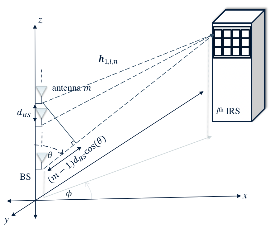
Figure 2: Model of $\mathbf{h}_{1,l,n}\in\mathbb{C}^{M\times 1}$ which is the $n^{th}$ column vector of of LoS BS-IRS $l$ channel matrix $\mathbf{H}_{1,l}$. The signals from transmit antennas arrive almost in parallel at the $n^{th}$ IRS element.

Assuming a uniform linear array (ULA) at the BS and uniform planar array (UPA) at the IRSs depicted in Fig. 2, the LoS BS-IRS $l$ channel can be written as

$$\mathbf{H_{1,l}}=\sqrt{\beta_{1,l}}\mathbf{a}_{l}\mathbf{b}_{l}^{H}.$$ (7)

Here, $\beta_{1,l}$ is the path loss factor for BS-IRS $l$ channel, $\mathbf{a}_{l}$ is the array response vector for the BS, while $\mathbf{b}_{l}$ is the array response vector for IRS $l$. The vector $\mathbf{a}_{l}\in\mathbb{C}^{M\times 1}$ is written as [24]

$$\mathbf{a}_{l}=[1,e^{-jkd_{BS}\cos(\theta_{l})},\dots,e^{-jkd_{BS}(M-1)\cos(\theta_{l})}]^{T},$$ (8)

where $d_{BS}$ is the inter-antenna spacing, $k=2\pi/\lambda_{c}$ is the wave number, $\lambda_{c}$ is carrier wavelength, $\theta_{l}$ is the elevation AoD from the BS to IRS $l$ (cf. Fig.2).

The IRS is envisioned to be a planar array of $N=N_{x}N_{z}$ elements, where $N_{x}$ and $N_{z}$ denote the number of horizontally and vertically placed elements, respectively. The array response vector $\mathbf{b}_{l}\in\mathbb{C}^{N\times 1}$ for a UPA at IRS $l$ is expressed as to be $\mathbf{b}_{l}=\mathbf{b}_{l,x}^{T}\otimes\mathbf{b}_{l,z}^{T}$ and [25]

$$\mathbf{b}_{l,x}=[1,e^{-jkd_{IRS}\sin(\varphi_{l})cos(\vartheta_{l})},\dots,e^{-jkd_{IRS}(N_{x}-1)\sin(\varphi_{l})cos(\vartheta_{l})}],$$ (9)

$$\mathbf{b}_{l,z}=[1,e^{-jkd_{IRS}cos(\varphi_{l})},\dots,e^{-jkd_{IRS}(N_{z}-1)cos(\varphi_{l})}],$$ (10)

where $d_{IRS}$ is the inter-element spacing, and $\vartheta_{l}$ $(\varphi_{l})$ denote the azimuth (elevation) AoA of the path from BS to IRS $l$ [26]. It is apparent that each BS-IRS $l$ channel matrix has a rank one structure, thus $\mathbf{H}_{1,l}$ is a rank-one matrix with a unique non-zero singular value $\lambda_{\mathbf{H}_{1,l}}=\sqrt{\beta_{1,l}}$ [24]. The rank one assumption is accurate since the elements at both the BS and IRSs are co-located and the IRSs are assumed to be in the far-field, i.e., the propagation distance $d_{BS-IRS_{l}}$ between the BS and IRS $l$ is much larger than the largest dimension of that IRS. Although a channel with rank one means only one degree of freedom for the system, with distributed surfaces the overall channel between BS and each user will at least have rank $L$, which allows multiple users to be served simultaneously.

II-C Problem Statement

We focus on the average (ergodic) analysis of the SINR at each user in the distributed IRSs-assisted multi-user MISO system, where each IRS is associated with a user in the system. For a particular IRS-user association pair, we choose the design for IRS phase shifts that would maximize the received signal strength at that user. Under that design, we utilize statistical tools to obtain a closed form expression for the average SINR at each user. Therefore, we develop an average SINR expression under IRS-user association parameters, optimized IRS passive beamforming, and MRT precoding at the BS. Next, we formulate and solve a max-min average SINR optimization problem to find the optimal IRS-user association parameters.

III Downlink SINR Analysis

With distributed IRSs deployed in a multi-user system, we consider associating IRSs to different users in an optimal manner to achieve a desired performance objective such as max-min average SINR in this work. We assume that each IRS will be associated with and therefore tuned to a single user. The motivation behind single-user association with an IRS is that it is user-centric and simplifies the optimal phase shifts design since the design can be based on the local CSI of the associated user, thus reducing complexity. A future research direction can be to consider the setting where each IRS is associated to multiple users and is optimally tuned to serve those users. Using (2), the $k^{th}$ user receives

$$y_{k} =\mathbf{h}_{d,k}^{H}\mathbf{x}+\sum_{l=1}^{L}\mathbf{h}_{2,l,k}^{H}\boldsymbol{\Theta}_{l}^{H}\mathbf{H}_{1,l}^{H}\mathbf{x}+n_{k},$$ (11)

where the channels are given in (5), (6), and (7). To aid in expressing the instantaneous SINR $\gamma_{k}$ for user $k$, we rewrite $y_{k}$ as $y_{k}={y_{k}}_{D}+{y_{k}}_{I}$, where ${y_{k}}_{D}$ is the desired signal given by

$${y_{k}}_{D} =\sqrt{p}_{k}\mathbf{h}_{d,k}^{H}\mathbf{f}_{k}s_{k}+\sqrt{p}_{k}\sum_{l=1}^{L}\mathbf{h}_{2,l,k}^{H}\boldsymbol{\Theta}_{l}^{H}\mathbf{H}_{1,l}^{H}\mathbf{f}_{k}s_{k},$$ (12)

and ${y_{k}}_{I}$ is the interference and noise terms given by

$${y_{k}}_{I} =\sum_{t\neq k,t=1}^{K}\bigg{(}\sqrt{p}_{t}\mathbf{h}_{d,k}^{H}\mathbf{f}_{t}s_{t}+\sqrt{p}_{t}\sum_{l=1}^{L}\mathbf{h}_{2,l,k}^{H}\boldsymbol{\Theta}_{l}^{H}\mathbf{H}_{1,l}^{H}\mathbf{f}_{t}s_{t}\bigg{)}+n_{k},$$ (13)

Thus, we construct the SINR $\gamma_{k}$ at user $k$ under the transmission model just described as

$$\gamma_{k}=\frac{p_{k}\|\mathbf{h}^{H}_{k}\mathbf{f}_{k}\|^{2}}{\sum_{t\neq k,t=1}^{K}p_{t}\|\mathbf{h}^{H}_{k}\mathbf{f}_{t}\|^{2}+\sigma^{2}}.$$ (14)

The direct and IRS cascaded channels in the downlink can be rewritten collectively as

$$\mathbf{h}^{H}_{k} =\mathbf{h}_{d,k}^{H}+\sum_{l=1}^{L}\mathbf{h}_{2,l,k}^{H}\boldsymbol{\Theta}_{l}^{H}\mathbf{H}_{1,l}^{H}=\mathbf{h}_{d,k}^{H}+\sum_{l=1}^{L}\mathbf{v}_{l}^{H}\mathbf{H}_{0,l,k}^{H},$$ (15)

where

$$\mathbf{H}_{0,l,k}=\mathbf{H}_{1,l}\text{diag}(\mathbf{h}_{2,l,k})=\sqrt{\beta_{1,l}}\mathbf{a}_{l}\mathbf{b}_{l}^{H}\text{diag}(\mathbf{h}_{2,l,k})$$ (16)

and $\mathbf{v}_{l}=\text{diag}(\boldsymbol{\Theta}_{l})\in\mathbb{C}^{N\times 1}$. Using (15), we rewrite the instantaneous SINR $\gamma_{k}$ in (14) as

$$\gamma_{k}=\frac{p_{k}\|(\mathbf{h}_{d,k}^{H}+\sum_{l=1}^{L}\mathbf{v}_{l}^{H}\mathbf{H}_{0,l,k}^{H})\mathbf{f}_{k}\|^{2}}{\sum_{t\neq k,t=1}^{K}p_{t}\|(\mathbf{h}_{d,k}^{H}+\sum_{l=1}^{L}\mathbf{v}_{l}^{H}\mathbf{H}_{0,l,k}^{H})\mathbf{f}_{t}\|^{2}+\sigma^{2}}.$$ (17)

At this stage, we introduce the association variables $\lambda_{l,k}\in\{0,1\}$ which are binary variables denoting association between the $l^{th}$ IRS and $k^{th}$ user. Note that $\lambda_{l,k}=1$ when the $l^{th}$ IRS is associated to the $k^{th}$ user, and $\lambda_{l,k}=0$ when there is no association with that user. The overall channel in (15) with association variables can be reformulated as

$$\mathbf{h}^{H}_{k}(\boldsymbol{\lambda}_{k})=\mathbf{h}_{d,k}^{H}+\sum_{l=1}^{L}\lambda_{l,k}\mathbf{v}_{l}^{{k_{l}}^{H}}\mathbf{H}_{0,l,k}^{H}+\sum_{l=1}^{L}(1-\lambda_{l,k})\mathbf{v}_{l}^{k_{l}^{H}}\mathbf{H}_{0,l,k}^{H},$$ (18)

where $\boldsymbol{\lambda}_{k}\in\mathbb{B}^{1\times L}$ denotes the array of associated and/or non-associated IRSs with respect to user $k$ and is a row vector in $\boldsymbol{\Lambda\in\mathbb{B}^{K\times L}}$ which is the IRS-user association matrix. To make the association between the optimized (tuned) beamforming vector $\mathbf{v}_{l}$ to a particular user $k_{l}$, we replace $\mathbf{v}_{l}$ by $\mathbf{v}_{l}^{k_{l}}$ shown in (24) henceforth, where $k_{l}$ is the user for which $\lambda_{l,k_{l}}=1$. For (18), $k_{l}=k$ in the second term $\sum_{l=1}^{L}\lambda_{l,k}\mathbf{v}_{l}^{{k_{l}}^{H}}\mathbf{H}_{0,l,k}^{H}$ which means $\lambda_{l,k}=1$. As for the third term $\sum_{l=1}^{L}(1-\lambda_{l,k})\mathbf{v}_{l}^{k_{l}^{H}}\mathbf{H}_{0,l,k}^{H}$ we have $\mathbf{v}_{l}^{k_{l}}$ is the beamforming vector $\mathbf{v}_{l}$ of IRS $l$ optimized for associated user $k_{l}$ where $k_{l}\neq k$ such that $\lambda_{l,k_{l}}=1$ and $\lambda_{l,k}=0$. The notation $k_{l}$ is to ascertain an associated user $k_{l}$ which depends on its IRS association. In addition, we can rewrite (2) with association parameters as $y_{k}=\mathbf{h}^{H}_{k}(\boldsymbol{\lambda}_{k})\mathbf{x}+n_{k},$ and the updated, instantaneous SINR as

$$\gamma_{k}=\frac{p_{k}\|\mathbf{h}^{H}_{k}(\boldsymbol{\lambda}_{k})\mathbf{f}_{k}\|^{2}}{\sum_{t\neq k,t=1}^{K}p_{t}\|\mathbf{h}^{H}_{k}(\boldsymbol{\lambda}_{k})\mathbf{f}_{t}\|^{2}+\sigma^{2}}.$$ (19)

An important design goal is to optimize the downlink SINR in (19) with respect to the IRSs configuration, which we split into IRSs passive beamforming and IRS-user association. In the next section, we find the optimal reflect beamforming vector $\mathbf{v}_{l}^{k_{l}}$ at each IRS $l$ that would enhance the transmission quality to its associated user $k_{l}$.

III-A IRS Passive Beamforming

We find the optimal passive beamforming vector $\mathbf{v}_{l}^{k_{l}}$ for IRS $l$ associated with user $k_{l}$ such that $\lambda_{l,k_{l}}=1$, so as to maximize the channel gain via that IRS to that user. Note that finding $\mathbf{v}_{l}^{k_{l}}$ for each IRS $l$ such that SINR at its associated user $k_{l}$ is maximized will result in a highly intractable joint optimization problem involving the beamforming vectors of all IRSs and their association parameters with the users. There is no known closed-form optimal solution for $\mathbf{v}_{l}$ that maximizes the SINR, which is why we resort to maximizing the channel gain instead, similar to [14]. Hence, the passive beamforming optimization problem for an IRS $l$ associated with user $k_{l}$ can be defined as

$$(P0)\hskip 14.45377pt\underset{\mathbf{v}_{l}}{\text{max}} \hskip 14.45377pt\|\mathbf{h}_{d,k_{l}}^{H}+\mathbf{v}_{l}^{H}\mathbf{H}_{0,l,k_{l}}^{H}\|^{2}$$ (20)

$$\text{s.t.}\hskip 14.45377pt|v_{l,n}|=1.\forall n.$$ (21)

Here, $v_{l,n}$ denotes the $n^{th}$ element in $\mathbf{v}_{l}$, $\mathbf{h}_{d,k_{l}}$ and $\mathbf{H}_{0,l,k_{l}}$ are the direct and IRS cascaded channels for user $k_{l}$. Expanding the objective function yields $\|\mathbf{h}_{d,k_{l}}^{H}\|^{2}+2\langle\mathbf{v}_{l},\mathbf{H}_{0,l,k_{l}}^{H}\mathbf{h}_{d,k_{l}}\rangle+\|\mathbf{v}_{l}^{H}\mathbf{H}_{0,l,k_{l}}^{H}\|^{2}$, where we can drop the first term since it does not depend on the optimization variable to get

$$(P0^{\prime})\hskip 14.45377pt\underset{\mathbf{v}_{l}}{\text{max}}\hskip 14.45377pt 2\langle\mathbf{v}_{l},\mathbf{H}_{0,l,k_{l}}^{H}\mathbf{h}_{d,k_{l}}\rangle+\|\mathbf{v}_{l}^{H}\mathbf{H}_{0,l,k_{l}}^{H}\|^{2}$$ (22)

$$\text{s.t.}\hskip 14.45377pt|v_{l,n}|=1.\forall n.$$ (23)

Lemma 1

The optimal solution of $(P0^{\prime})$ for the beamforming vector of IRS $l$ associated with user $k_{l}$, such that $\lambda_{l,k_{l}}=1$ is

$$\mathbf{v}_{l}^{k_{l}}=e^{j\angle{\text{diag}(\mathbf{h}^{H}_{2,l,k_{l}})\mathbf{b}_{l}}}e^{j\angle{\mathbf{a}_{l}^{H}\mathbf{h}_{d,k_{l}}}}.$$ (24)

Proof:

It suffices to express $\langle\mathbf{v}_{l},\mathbf{H}_{0,l,k_{l}}^{H}\mathbf{h}_{d,k_{l}}\rangle=\sum_{n=1}^{N}|v_{l,n}||{h_{m}}|\cos(\angle v_{l,n}-\angle h_{m})$, where $v_{l,n}$ (${h}_{m}$) is the $n^{th}$ component of $\mathbf{v}_{l}$ ($\mathbf{H}_{0,l,k_{l}}^{H}\mathbf{h}_{d,k_{l}}$). This expression achieves its maximum value when $\angle v_{l,n}^{k_{l}}=\angle{h}_{m}$, equivalently ($\angle\mathbf{v}_{l}^{k_{l}}=\angle\text{diag}(\mathbf{h}_{2,l,k_{l}}^{H})\mathbf{b}_{l}\mathbf{a}_{l}^{H}\mathbf{h}_{d,k_{l}})$ where $v_{l,n}^{k_{l}}$ is the $n^{th}$ element of $\angle\mathbf{v}_{l}^{k_{l}}$, which is solution presented in (24) in simplified form. Similar argument can be done for the second term in the objective function (22), where $\underset{\mathbf{v}_{l}}{\text{max}}\hskip 14.45377pt\|\mathbf{v}_{l}^{H}\mathbf{H}_{0,l,k_{l}}^{H}\|^{2}$

$$=\underset{\mathbf{v}_{l}}{\text{max}}\hskip 14.45377pt\mathbf{v}_{l}^{H}\text{diag}(\mathbf{h}_{2,l,k_{l}}^{H})\mathbf{b}\mathbf{a}^{H}\mathbf{a}\mathbf{b}^{H}\text{diag}(\mathbf{h}_{2,l,k_{l}})\mathbf{v}_{l}=\underset{\mathbf{v}_{l}}{\text{max}}\hskip 14.45377pt\|\mathbf{a}_{l}\|^{2}|\mathbf{v}_{l}^{H}\text{diag}(\mathbf{h}_{2,l,k_{l}}^{H})\mathbf{b}_{l}|^{2},$$ (25)

$$=\|\mathbf{a}_{l}\|^{2}\bigg{|}\sum_{n=1}^{N}|{v}^{k}_{l,n}||{h}_{2,l,k_{l},n}||{b}_{l,n}|e^{j({\angle{h_{2,l,k_{l},n}}+\angle{b^{*}_{l,n}}+\angle{h^{*}_{2,l,k_{l},n}}+\angle{b_{l,n}}}+\angle{\mathbf{h}_{d,k_{l}}^{H}\mathbf{a}_{l}})}\bigg{|}^{2},$$ (26)

$$=\|\mathbf{a}_{l}\|^{2}(\sum_{n=1}^{N}|{h}_{2,l,k_{l},n}||{b}_{l,n}|)^{2}|e^{j(\angle{\mathbf{h}_{d,k_{l}}^{H}\mathbf{a}_{l}})}|^{2}=\|\mathbf{a}_{l}\|^{2}(\sum_{n=1}^{N}|{h}_{2,l,k_{l},n}||{b}_{l,n}|)^{2}.$$ (27)

Here, (27) is obtained by noting that there is a unit-modulus constraint on $v_{l,n}$, i.e., $|v_{l,n}|=1$. Moreover, the last line is found by recalling that the absolute square of a complex number is the complex number multiplied by its conjugate, i.e., $|e^{j(\angle{\mathbf{h}_{d,k_{l}}^{H}\mathbf{a}_{l}})}|^{2}=e^{j(\angle{\mathbf{h}_{d,k_{l}}^{H}\mathbf{a}_{l}})}e^{-j(\angle{\mathbf{h}_{d,k_{l}}^{H}\mathbf{a}_{l}})}=e^{j(\angle{\mathbf{h}_{d,k_{l}}^{H}\mathbf{a}_{l}}-\angle{\mathbf{h}_{d,k_{l}}^{H}\mathbf{a}_{l}})}=1$. Finally, the expression achieves its maximum value when the argument of all the complex numbers involved cancel each other which is accomplished with the choice of reflection beamforming vector given in (24). ∎

Next, we turn our attention to obtaining the closed-form expression for the average SINR at each user in (19) under the IRS passive beamforming design in (24).

III-B Average SINR

Since practical wireless channels undergo random fading, an important performance metric is the average SINR $\bar{\gamma}_{k}$ which depends only on statistics of the channels. Channel statistics such as path loss and correlation matrices change slowly as compared to the fast fading channels themselves. Therefore, instead of computing instantaneous SINR in each coherence interval, $\bar{\gamma}_{k}$ can be used as a performance metric to optimize the system. In fact, by using $\bar{\gamma}_{k}$ as a performance metric, the IRS-user association parameters will not need to be updated on the coherence time scale but only when the large-scale statistics of the channels change. Once the association is established, the BS will use local CSI of the associated user to determine each IRS’s optimal configuration in (24). Next, we present the approximation of the average SINR in Lemma 2.

Lemma 2

The average SINR $\bar{\gamma}_{k}=\mathbb{E}[\gamma_{k}]$, with $\gamma_{k}$ given by (19) is approximated as [27], [28]

$$\bar{\gamma}_{k}=\mathbb{E}[\gamma_{k}]\approx\frac{p_{k}\mathbb{E}[\|\mathbf{h}^{H}_{k}(\boldsymbol{\lambda}_{k})\mathbf{f}_{k}(\boldsymbol{\lambda}_{k})\|^{2}]}{\sum_{t\neq k,t=1}^{K}p_{t}\mathbb{E}[\|\mathbf{h}^{H}_{k}(\boldsymbol{\lambda}_{k})\mathbf{f}_{t}(\boldsymbol{\lambda}_{t})\|^{2}]+\sigma^{2}}$$ (28)

Proof:

Consider the expectation $\mathbb{E}[\frac{X}{Y}]$ and assume $\mathbb{E}[X]=\mu_{X}$ and $\mathbb{E}[Y]=\mu_{Y}$. We can expand the ratio $\frac{X}{Y}$ (using the bivariate first-order Taylor series expansion) around the point $(\mu_{X},\mu_{Y})$ so that

$$\frac{X}{Y}=\frac{\mu_{X}}{\mu_{Y}}+\frac{1}{\mu_{Y}}(X-\mu_{X})-\frac{\mu_{X}}{\mu_{Y}^{2}}(Y-\mu_{Y})+C$$ (29)

where $C$ denotes the remaining higher-order terms in the expansion. Taking the first moment of this ratio provides

$$\mathbb{E}\left[\frac{X}{Y}\right]=\mathbb{E}\left[\frac{\mu_{X}}{\mu_{Y}}+\frac{1}{\mu_{Y}}(X-\mu_{X})-\frac{\mu_{X}}{\mu_{Y}^{2}}(Y-\mu_{Y})+C\right]$$ (30)

$$\underset{(i)}{\approx}\mathbb{E}\left[\frac{\mu_{X}}{\mu_{Y}}\right]+\mathbb{E}\left[\frac{1}{\mu_{Y}}(X-\mu_{X})\right]-\mathbb{E}\left[\frac{\mu_{X}}{\mu_{Y}^{2}}(Y-\mu_{Y})\right]\underset{(ii)}{=}\frac{\mathbb{E}[X]}{\mathbb{E}[Y]}$$ (31)

where $(i)$ follows from dropping the higher order terms $C$, and $(ii)$ follows since the expectation of the second and third terms is zero. Applying this to $\mathbb{E}[\gamma_{k}]$ yields (28). ∎

This approximation of average SINR is very tight as will be verified numerically in Fig. 5 in the simulation results. Substituting the MRT precoder (4) in (28) yields

$$\bar{\gamma}_{k}=\frac{p_{k}\frac{\mathbb{E}[\|\mathbf{h}^{H}_{k}(\boldsymbol{\lambda}_{k})\|^{4}]}{\mathbb{E}[\|\mathbf{h}^{H}_{k}(\boldsymbol{\lambda}_{k})\|^{2}]}}{\sum_{t\neq k,t=1}^{K}p_{t}\frac{\mathbb{E}[\|\mathbf{h}^{H}_{k}(\boldsymbol{\lambda}_{k})\mathbf{h}_{t}(\boldsymbol{\lambda}_{t})\|^{2}]}{\mathbb{E}[\|\mathbf{h}^{H}_{t}(\boldsymbol{\lambda}_{t})\|^{2}]}+\sigma^{2}}$$ (32)

III-C Main Results

Before we present the main derivation for the average SINR, note that the channel $\mathbf{h}_{k}(\boldsymbol{\lambda}_{k})$ in (18) is distributed as $\mathbf{h}_{k}(\boldsymbol{\lambda}_{k})\sim\mathcal{CN}(0,\mathbf{R}_{k})$ since it contains the addition of complex Gaussian vectors. As a result, $\mathbf{h}_{k}(\boldsymbol{\lambda}_{k})$ is a complex Gaussian vector with zero mean and correlation matrix $\mathbf{R}_{k}$, which will be derived later in this section.

In this section, we derive all the expectations in (32), which would require us to find the first and second moments of a complex Gaussian quadratic form abbreviated as (CGQF). First, we expand the expectation of the squared channel gain as

$$\mathbb{E}[\|{\mathbf{h}}_{k}(\boldsymbol{\lambda}_{k})\|^{2}]=\mathbb{E}[\mathbf{h}_{d,k}^{H}\mathbf{h}_{d,k}+2\sum_{l=1}^{L}\lambda_{l,k}\mathbf{v}_{l}^{{k_{l}}^{H}}\mathbf{H}_{0,l,k}^{H}\mathbf{h}_{d,k}+$$ (33)

$$\sum_{l=1}^{L}\sum_{\bar{l}=1}^{L}\lambda_{l,k}\lambda_{\bar{l},k}\mathbf{v}_{l}^{{k_{l}}^{H}}\mathbf{H}_{0,l,k}^{H}\mathbf{H}_{0,\bar{l},k}\mathbf{v}_{\bar{l}}^{{k_{\bar{l}}}}+\sum_{l=1}^{L}\sum_{\bar{l}=1}^{L}(1-\lambda_{l,k})(1-\lambda_{\bar{l},k})\mathbf{v}_{l}^{k_{l}^{H}}\mathbf{H}_{0,l,k}^{H}\mathbf{H}_{0,\bar{l},k}\mathbf{v}_{\bar{l}}^{{k_{\bar{l}}}}$$

$$+2\sum_{l=1}^{L}(1-\lambda_{l,k})\mathbf{v}_{l}^{k_{l}^{H}}\mathbf{H}_{0,l,k}^{H}\mathbf{h}_{d,k}+2\sum_{l=1}^{L}\sum_{\bar{l}=1}^{L}(1-\lambda_{\bar{l},,k})\lambda_{{l,k}}\mathbf{v}_{l}^{{k_{l}}^{H}}\mathbf{H}_{0,l,k}^{H}\mathbf{H}_{0,\bar{l},k}\mathbf{v}_{\bar{l}}^{{k_{\bar{l}}}}],$$

where $\mathbf{v}^{k_{l}}_{l}$ and $\mathbf{v}^{k_{\bar{l}}}_{\bar{l}}$ are of the form in (24) for user $k_{l}$ associated with IRS $l$ and user $k_{\bar{l}}$ associated with IRS $\bar{l}$, respectively. Note that the last two terms in (33) are zero due to independence between channels $\mathbf{h}_{2,l,k}$’s and $\mathbf{h}_{d,k}$’s. Next we present this expectation in a closed form in the following lemma.

Lemma 3

The expectation in (33) is given by

$$\mathbb{E}[\|{\mathbf{h}}_{k}(\boldsymbol{\lambda}_{k})\|^{2}]= M\beta_{d,k}+\sum_{l=1}^{L}\lambda_{l,k}\bigg{(}\alpha+tr(\mathbf{H}_{1,l}^{H}\mathbf{H}_{1,{l}}\boldsymbol{\Sigma}_{\tilde{\mathbf{v}}_{l}^{k_{l}}}-\beta_{2,l,k}\mathbf{H}_{1,l}^{H}\mathbf{H}_{1,{l}})\bigg{)}$$

$$+\beta_{2,l,k}tr(\mathbf{H}_{1,l}^{H}\mathbf{H}_{1,{l}}),$$ (34)

where $\alpha=\sqrt{\beta_{1,l}\beta_{2,l,k}\beta_{d,k}}\frac{\pi\sqrt{M}{N}}{2}$ and $\boldsymbol{\Sigma}_{\tilde{\mathbf{v}}_{l}^{k_{l}}}=\beta_{2,l,k}\mathbf{I}_{N}+\frac{\pi\beta_{2,l,k}}{4}\mathbf{e}^{j\angle\mathbf{H}_{1,l}^{H}\mathbf{H}_{1,l}}\odot(\mathbf{1}_{N}-\mathbf{I}_{N})$.

Proof:

The proof is postponed to Appendix A. ∎

Note that $\mathbb{E}[\|{\mathbf{h}}_{k}(\lambda_{l,k})\|^{2}]=tr(\mathbf{R}_{k})$. The term in $\mathbb{E}[\|{\mathbf{h}}_{k}(\boldsymbol{\lambda}_{k})\|^{2}]$ accounting for the gains from non-associated IRSs is $\sum_{l=1}^{L}(1-\lambda_{l,k})\beta_{2,l,k}tr(\mathbf{H}_{1,l}^{H}\mathbf{H}_{1,{l}})$ which has been distributed for a more concise representation in (3). It can be seen that the average squared channel gain increases with respect to $M$. On the other hand, the average squared channel gain depends on the user association parameters as well as $L$ and $N$. For instance, if user $k$ does not have any IRSs associated to it, i.e. $\lambda_{l,k}=0,\forall l$, then we still gain from all the non-associated IRSs although they are optimized for other users. Next we present in Lemma 4 the expression of $\mathbb{E}[\|{\mathbf{h}}_{k}(\lambda_{l,k})\|^{4}]$, which will be used to complete the analysis of the numerator of $\bar{\gamma}_{k}$.

Lemma 4

The fourth moment $\mathbb{E}[\|{\mathbf{h}}_{k}(\lambda_{l,k})\|^{4}]$ in the numerator of $\bar{\gamma}_{k}$ in (32) is derived using a result on the second moment of CGQF as

$$\mathbb{E}[\|{\mathbf{h}}_{k}(\boldsymbol{\lambda}_{k})\|^{4}]=tr(\mathbf{R}_{k}^{2})+tr(\mathbf{R}_{k})^{2}.$$ (35)

Proof:

$$\mathbb{E}[\|{\mathbf{h}}_{k}(\boldsymbol{\lambda}_{k})\|^{4}]=\text{Var}[\|{\mathbf{h}}_{k}(\boldsymbol{\lambda}_{k})\|^{2}]+(\mathbb{E}[\|{\mathbf{h}}_{k}(\boldsymbol{\lambda}_{k})\|^{2}])^{2}$$ (36)

$$=\text{Var}[\|{\mathbf{h}}_{k}(\boldsymbol{\lambda}_{k})\|^{2}]+tr(\mathbf{R}_{k})^{2}=tr(\mathbf{R}_{k}^{2})+tr(\mathbf{R}_{k})^{2},$$ (37)

where $\text{Var}[\|{\mathbf{h}}_{k}(\boldsymbol{\lambda}_{k})\|^{2}]=tr(\mathbf{R}_{k}^{2})$ follows from the second moment of a CGQF [29], [27].

∎

One can see from Lemma 4 that this result relies heavily on the correlation matrix $\mathbf{R}_{k}$, as its diagonal elements become larger so does the channel gain. In fact, increasing $M$ increases the fourth-order moment in (35) quadratically. However, increasing the size of the diagonal elements of $\mathbf{R}_{k}$ also affects the interference as seen below.

Next we present in Lemma 5 the expression of $\mathbb{E}[\|\mathbf{h}_{k}^{H}(\boldsymbol{\lambda}_{k})\mathbf{h}_{t}(\boldsymbol{\lambda}_{t})\|^{2}]$ which appears in the interference term in (32).

Lemma 5

In the interference term $\sum_{t\neq k,t=1}^{K}p_{t}\frac{\mathbb{E}[\|\mathbf{h}^{H}_{k}(\boldsymbol{\lambda}_{k})\mathbf{h}_{t}(\boldsymbol{\lambda}_{t})\|^{2}]}{\mathbb{E}[\|\mathbf{h}^{H}_{t}(\boldsymbol{\lambda}_{t})\|^{2}]}$, the numerator is found to be

$$\mathbb{E}[\|\mathbf{h}_{k}^{H}(\boldsymbol{\lambda}_{k})\mathbf{h}_{t}(\boldsymbol{\lambda}_{t})\|^{2}]=tr(\mathbf{R}_{t}\mathbf{R}_{k}).$$ (38)

Proof:

$$\mathbb{E}[\|\mathbf{h}_{k}^{H}(\boldsymbol{\lambda}_{k})\mathbf{h}_{t}(\boldsymbol{\lambda}_{t})\|^{2}]=\mathbb{E}[\mathbf{h}_{k}^{H}(\boldsymbol{\lambda}_{k})\mathbf{h}_{t}(\boldsymbol{\lambda}_{t})\mathbf{h}_{t}^{H}(\boldsymbol{\lambda}_{t})\mathbf{h}_{k}(\boldsymbol{\lambda}_{k})].$$ (39)

Since $\mathbf{h}_{t}(\boldsymbol{\lambda}_{t})$ and $\mathbf{h}_{k}(\boldsymbol{\lambda}_{k})$ are independent, we can use conditional expectation as

$$\mathbb{E}_{\mathbf{h}_{k}}[\mathbf{h}_{k}^{H}(\lambda_{l,k})\mathbb{E}_{\mathbf{h}_{t}}[\mathbf{h}_{t}(\lambda_{l,k})\mathbf{h}_{t}^{H}(\lambda_{l,k})|\mathbf{h}_{k}(\lambda_{l,k})]\mathbf{h}_{k}(\lambda_{l,k})]=\mathbb{E}_{\mathbf{h}_{k}}[\mathbf{h}_{k}^{H}(\lambda_{l,k})\mathbf{R}_{t}\mathbf{h}_{k}(\lambda_{l,k})],$$ (40)

$$=\mathbb{E}_{\mathbf{h}_{k}}[tr(\mathbf{h}_{k}^{H}(\lambda_{l,k})\mathbf{R}_{t}\mathbf{h}_{k}(\lambda_{l,k}))]=\mathbb{E}_{\mathbf{h}_{k}}[tr(\mathbf{R}_{t}\mathbf{h}_{k}(\lambda_{l,k})\mathbf{h}^{H}_{k}(\lambda_{l,k}))],$$ (41)

$$=tr(\mathbf{R}_{t}\mathbb{E}_{\mathbf{h}_{k}}[\mathbf{h}_{k}(\lambda_{l,k})\mathbf{h}^{H}_{k}(\lambda_{l,k})])=tr(\mathbf{R}_{t}\mathbf{R}_{k}).$$ (42)

The denominator of the interference term is derived in Lemma 3, previously. ∎

To obtain expressions in (35) and (38) we need to find the expression for $\mathbf{R}_{k}$ which is next computed. Define the correlation matrix for $\mathbf{h}_{k}$ to be

$$\mathbf{R}_{k}= \mathbb{E}[{\mathbf{h}}_{k}(\boldsymbol{\lambda}_{k}){\mathbf{h}}_{k}(\boldsymbol{\lambda}_{k})^{H}]=\mathbb{E}[\mathbf{h}_{d,k}\mathbf{h}_{d,k}^{H}+2\sum_{l=1}^{L}\lambda_{l,k}\mathbf{h}_{d,k}\mathbf{v}_{l}^{{k_{l}}^{H}}\mathbf{H}_{0,l,k}^{H}$$ (43)

$$+\sum_{l=1}^{L}\sum_{\bar{l}=1}^{L}\lambda_{l,k}\lambda_{\bar{l},k}\mathbf{H}_{0,l,k}\mathbf{v}_{l}^{k_{l}}\mathbf{v}_{\bar{l}}^{{k_{\bar{l}}}^{H}}\mathbf{H}_{0,\bar{l},k}^{H}+\sum_{l=1}^{L}\sum_{\bar{l}=1}^{L}(1-\lambda_{l,k})(1-\lambda_{\bar{l},k})\mathbf{H}_{0,l,k}\mathbf{v}_{l}^{k_{l}}\mathbf{v}_{\bar{l}}^{k_{\bar{l}}^{H}}\mathbf{H}_{0,\bar{l},k}^{H}],$$

where other terms are zeros as shown in Appendix A. The expression given in the next lemma for $\mathbf{R}_{k}$ depends on the system dimensions $M,N,L$, path loss factors $\beta_{1,l},\beta_{2,l,k},\beta_{d,k}$, and association parameters $\lambda_{l,k}$s. In Sec. III-B, we optimize the association parameter matrix $\boldsymbol{\Lambda}$ as to maximize the minimum $\bar{\gamma}_{k}$.

Lemma 6

The correlation matrix for channel $\mathbf{h}_{k}(\boldsymbol{\lambda}_{k})$ in (18) is shown to be

$$\mathbf{R}_{k}= \beta_{d,k}\mathbf{I}_{M}+\sum_{l=1}^{L}\lambda_{l,k}\bigg{(}2\sqrt{\beta_{1,l}\beta_{2,l,k}\beta_{d,k}}\frac{N\pi}{4\sqrt{M}}\mathbf{e}^{j\angle\mathbf{H}_{1,l}\mathbf{H}_{1,l}^{H}}$$ (44)

$$+\mathbf{H}_{1,l}\boldsymbol{\Sigma}_{\tilde{\mathbf{v}}_{l}^{k_{l}}}\mathbf{H}_{1,l}^{H}-\beta_{2,l,k}\mathbf{H}_{1,l}\mathbf{H}_{1,{l}}^{H}\bigg{)}+\sum_{l=1}^{L}\beta_{2,l,k}\mathbf{H}_{1,l}\mathbf{H}_{1,{l}}^{H}.$$

Proof:

The proof is postponed to Appendix B. ∎

Now, we can combine these results in the following Theorem 1 to find a closed-form expression for the average SINR at user $k$.

Theorem 1

Using the results from Lemmas 3, 4, 5, the ergodic SINR under MRT and IRS passive beamforming in (24) for a given IRS-user association matrix $\boldsymbol{\Lambda}$ is given as

$$\bar{\gamma}_{k}=\frac{\frac{p_{k}}{tr(\mathbf{R}_{k})}\big{(}tr(\mathbf{R}_{k}^{2})+tr(\mathbf{R}_{k})^{2}\big{)}}{\sum_{t\neq k,t=1}^{K}\frac{p_{t}}{tr(\mathbf{R}_{t})}tr(\mathbf{R}_{t}\mathbf{R}_{k})+\sigma^{2}}=\frac{{c_{k}}(tr(\mathbf{R}_{k}^{2})+tr(\mathbf{R}_{k})^{2})}{\sum_{t\neq k,t=1}^{K}{c_{t}}tr(\mathbf{R}_{t}\mathbf{R}_{k})+\sigma^{2}},$$ (45)

where $c_{k}$ satisfies ${p_{k}}=c_{k}tr(\mathbf{R}_{k})\forall k$, and $\mathbf{R}_{k}$ is defined in (44) as a function of $\boldsymbol{\Lambda}$.

Corollary 1

When the correlation matrices of different users are orthogonal, i.e. $\mathbf{R}_{t}\mathbf{R}_{k}=\mathbf{0}_{M}$, then the average SINR in (45) simplifies to an average SINR upper bound given by

$$\bar{\gamma}_{k,Up}=\frac{{c_{k}}(tr(\mathbf{R}_{k}^{2})+tr(\mathbf{R}_{k})^{2})}{\sigma^{2}}$$ (46)

When the correlation matrices of all users are identical and the allocated powers for all users are the same, i.e., $\mathbf{R}_{t}=\mathbf{R}_{k}=\mathbb{E}[{\mathbf{h}}_{k}(\boldsymbol{\lambda}_{k}){\mathbf{h}}_{k}(\boldsymbol{\lambda}_{k})^{H}]$ [30], and $p_{1}=p_{2}=\dots=p_{K}$, the average SINR simplifies to the following average SINR lower bound

$$\bar{\gamma}_{k,Low}=\frac{1+tr(\mathbf{R}_{k})^{2}/tr(\mathbf{R}_{k}^{2})}{(K-1)+\sigma^{2}/c_{k}tr(\mathbf{R}_{k}^{2})}.$$ (47)

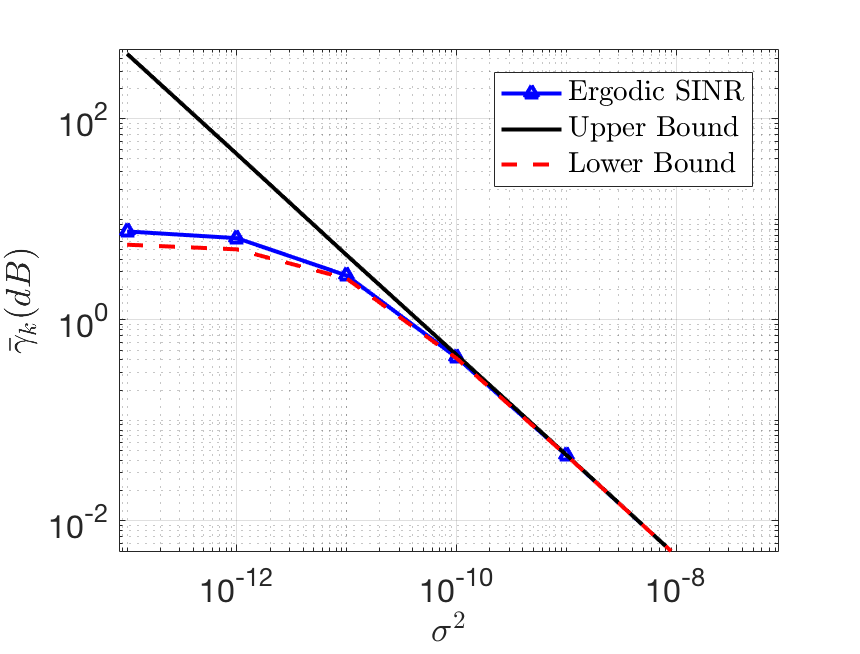
Essentially, Corollary 1 presents meaningful bounds $\bar{\gamma}_{k,Low}\leq\bar{\gamma}_{k}\leq\bar{\gamma}_{k,Up}$ which are illustrated in Fig. 5 in the simulations in Sec. IV, that show how the level of diversity between correlation matrices of different users impacts the average SINR. Having diverse channels lends to a higher overall SINR, while having users with similar correlation matrices leads to a degradation in SINR performance. In the next section, we formulate the max-min SINR problem using the average SINR derived in (45) to find the optimal IRS-user association pairs.

IV IRS-User Association Optimization Problem

The design of beamforming in literature is often based on two common optimization criteria— the transmit power minimization and the maximization of the minimum (max-min) SINR. The first criterion has been the focus of several works, while the latter was dealt with in [2] for a single IRS system and in [14] for a multi IRS system with single antenna transmitter.

To design the IRS-user association parameters for the considered multi-antenna multi-user IRSs-assisted system, we consider max-min average SINR as the performance metric to improve the performance and fairness of the system. We can formulate the max-min average SINR problem using the average SINR expression in (45) as

$$(P1)\hskip 14.45377pt \underset{\mathbf{\Lambda}}{\text{max}}\hskip 14.45377pt\underset{k}{\text{min}}\hskip 14.45377pt\bar{\gamma}_{k}$$ (48)

$$s.t.\hskip 14.45377pt \sum_{k=1}^{K}\lambda_{l,k}=1,1\leq l\leq L,$$ (49)

$$\lambda_{l,k}\in\{0,1\},1\leq l\leq L,1\leq k\leq K,$$ (50)

where $\boldsymbol{\Lambda}\in\mathbb{B}^{K\times L}$ denotes the binary association matrix between the $K$ users and $L$ IRSs, where each element $\lambda_{l,k}$ can take the value zero or one as mentioned in constraint (50).The constraint (49) limits each IRS to be associated to only one user. The binary constraint in (50) makes this problem a non-convex mixed-integer non-linear programming (MINLP) problem, which is NP-hard. We can find the optimal solution for the association parameters by exhaustive search, but the complexity is prohibitive and in the order $\mathcal{O}(K^{L})$. In the next subsections, we define the search space (codebook) for the exhaustive search method and outline a low-complexity SR algorithm.

IV-1 Exhaustive Search

In exhaustive search, we find the IRS-user association matrix that maximizes the minimum SINR over all possible IRS-user association matrices taken from a specific codebook. To create the codebook $C\in\mathbb{B}^{K\times L\times K^{L}}$ that can generate all possible $K^{L}$ combinations of $\mathbf{\Lambda}$, we define the rules according to $(P1)$ as:

1. Each IRS $l$ is associated to only one user $k$.

2. $\lambda_{l,k}$ is a binary variable.

We assign a number $N\in\mathbb{Z}^{+}$, where $N$ can take values from ${1,\dots,K^{L}}$ to uniquely represent each matrix $\mathbf{\Lambda}_{N}$. We then find the base $K$ representation of $N$ and store it in a row vector $\mathbf{r}$ which is of size $(L+1)\times 1$. The first $L$ elements of $\mathbf{r}$ which can only take on values ranging from $k=0,\dots,K-1$ by definition of base $K$ conversion, map to $L$ vectors each denoted by $\boldsymbol{\lambda}_{l}\in\mathbb{B}^{K\times 1}$. Each element $\mathbf{r}[l],l=1,\dots,L$ denotes the position index $i=\mathbf{r}[l]+1$ of $1$ in its corresponding $\boldsymbol{\lambda}_{l}$ such that $\boldsymbol{\lambda}_{l}[i]=1$ , where the rest of $\boldsymbol{\lambda}_{l}$’s elements are zeros. Thus, these $L$ $\boldsymbol{\lambda}_{l}$ columns are assembled as $\boldsymbol{\Lambda}_{N}$.

Example: For clarity, we give an example with $K=2,L=2$. The number of association matrices to generate is $K^{L}=4$ and are shown in (51). When $N=1$, the binary conversion where the most significant bit is here unconventionally the left-most bit will be $\mathbf{r}=[1,0,0]$. This corresponds to having the index $(\mathbf{r}[1]+1=2)$ for one in $\boldsymbol{\lambda}_{1}=[0,1]^{T}$ and $(\mathbf{r}[2]+1=1)$ for one in $\boldsymbol{\lambda}_{2}=[1,0]^{T}$. Assembling $\boldsymbol{\lambda}_{1}$ and $\boldsymbol{\lambda}_{2}$ results in $\boldsymbol{\Lambda}_{1}$. We skip $N=2,N=3$ since they follow similarly. For $N=4$, the binary conversion is $\mathbf{r}=[0,0,1]$. This corresponds to the index $(\mathbf{r}[1]+1=1)$ for one in $\boldsymbol{\lambda}_{1}=[1,0]^{T}$ and $(\mathbf{r}[2]+1=1)$ for one in $\boldsymbol{\lambda}_{2}=[1,0]^{T}$. Assembling $\boldsymbol{\lambda}_{1},\boldsymbol{\lambda}_{2}$ results in $\boldsymbol{\Lambda}_{4}$.

$$\boldsymbol{\Lambda}_{1}=\begin{bmatrix}0&1\\ 1&0\end{bmatrix},\boldsymbol{\Lambda}_{2}=\begin{bmatrix}1&0\\ 0&1\end{bmatrix},\boldsymbol{\Lambda}_{3}=\begin{bmatrix}0&0\\ 1&1\end{bmatrix},\boldsymbol{\Lambda}_{4}=\begin{bmatrix}1&1\\ 0&0\end{bmatrix}$$ (51)

IV-2 SR Algorithm

Result: Optimized IRS-user association matrix $\mathbf{\Lambda}^{*}$;

Initialize $\mathbf{\Lambda}$ based on nearest distance rule;

Initialize $\mathbf{v}^{k_{l}}_{l}$ using (24); Compute $\bar{\gamma}_{k}$s in (45) based on $\mathbf{\Lambda}$ and $\mathbf{v}^{k_{l}}_{l}$;

Set the iteration number $i=1$ and set $state=true$ ;

while state is true do

       $k$ = $\text{arg min}_{k}(\bar{\gamma}_{k})$ (bottleneck user), $\bar{\gamma}_{\text{min}}(i)=\bar{\gamma}_{k}$;

       for $l=1:L$ do

             if $\lambda_{l,k}=0$ then

                   $\lambda_{l,k}=1$, $\lambda_{l,j}=0$, $j\neq k$, where $j$ is the index of previously associated user of IRS $l$;

                   Update $\bar{\gamma}_{k}$s, $k=1,\dots,K$;

                   Find $\tilde{\gamma}(l)=\text{min}_{k}(\bar{\gamma}_{k})$;

                   Reset $\lambda_{l,k}=0$, $\lambda_{l,j}=1$;

                  

             end if

            

       end for

      Find $\bar{l}$ = $\text{arg max}_{l}(\tilde{\gamma}(l))$, i.e. the best IRS to improve the minimum SINR;

       $\lambda_{\bar{l},k}=1$, $\lambda_{\bar{l},{j}}=0$, where $j$ is the index of previously associated user of IRS $\bar{l}$;

       Update $\bar{\gamma}_{k}$, $k=1,\dots,K$ and find $\bar{\gamma}_{\text{min}}(i+1)=\text{min}_{k}(\bar{\gamma}_{k})$;

       if $\bar{\gamma}_{\text{min}}(i+1)<\bar{\gamma}_{\text{min}}(i)$  then

             $state=false$, $\lambda_{\bar{l},k}=0$, $\lambda_{\bar{l},{j}}=1$;

            

       end if

      $i=i+1$;

end while

Algorithm 1 SR Algorithm to Solve $(P1)$

To observe the gains yielded by optimizing IRS-user associations with low computational complexity, we outline the SR algorithm to maximize the minimum SINR, which was first proposed in [14]. First, we initialize the association matrix $\boldsymbol{\Lambda}$ using an appropriate criteria, like associating IRSs based on the minimum distance to the users. Under this initialization, we compute the average SINRs for all users and find the weakest (or the bottleneck user) user, which has the lowest average SINR $\bar{\gamma}_{k}$. After that, we search for an IRS that will increase the average SINR of this bottleneck user while not decreasing the overall system’s minimum SINR. We iterate in this manner until there can be no further improvement in the minimum average SINR of the system. The SR algorithm is summarized in Algorithm 1. This method has a complexity in the order of $\mathcal{O}(L)$. The minimum average SINR performance under SR algorithm matches closely to that under the optimal solution yielded by exhaustive search as shown in the simulation results.

V Numerical Simulations and Discussion

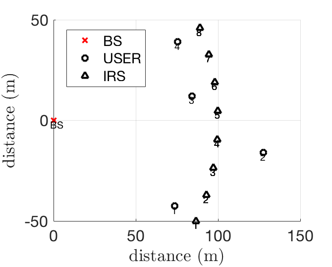
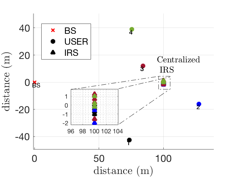
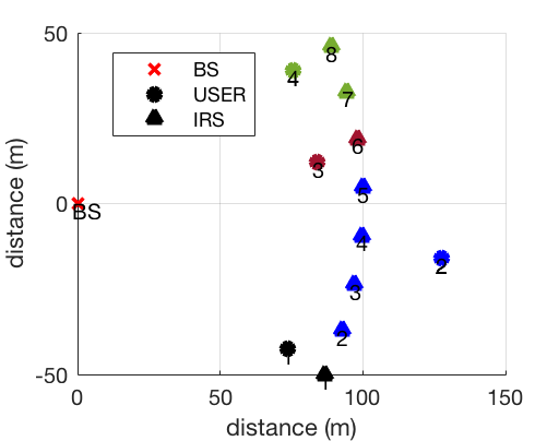
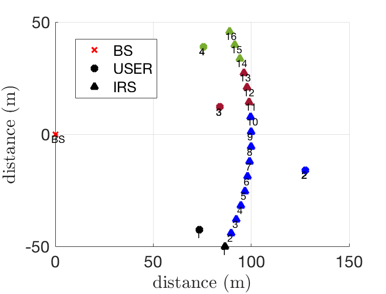
The parameter values for the simulation results in this section are tabulated in Table 3(a). We consider the following deployment. Denoting by $(x,y)$ the Cartesian coordinates, the BS is located at $(0,0)m$, the $L$ IRSs are deployed on an arc of radius $100m$ with respect to the BS, and the $K$ users are distributed on an arc of radius $85m$ with one user (numbered 2) is set further away at a radius of $130m$. This distributed IRSs deployment is illustrated in Fig. 3(b) and the user $2$ is deliberately positioned further away to highlight how the proposed IRS-user association algorithm helps the edge (or bottleneck) users.

Parameter	Value
Array parameters:
BS configuration	Uniform linear array
IRS configuration	Uniform planar array
Antenna gain	5dBi
$d_{BS}$, $d_{IRS}$	$0.5\lambda$
Noise level	$-60$dBm
Path Loss:
Model	$\frac{10^{-C/10}}{d^{\alpha}}$
$C$ (Fixed loss at $d=1$m)	$25$dB ($\beta_{1}$), $30$dB ($\beta_{2,k},\beta_{d,k}$)
$\alpha$ (Path loss exponent)	$2.2$ ($\beta_{1}$), $3.67$ ($\beta_{2,k},\beta_{d,k}$)
Penetration Loss:
$(\mathbf{h}_{d,k},\mathbf{h}_{2,l,k})$	($20$dB, $5$dB)
System Dimensions:
$(L,K,M)$	$(8,4,16)$

(a)

(b)

Figure 3: Deployment scenario and parameters.

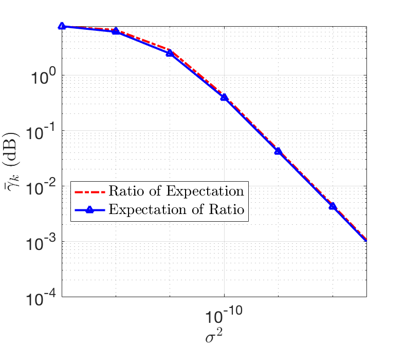
The path loss factors are computed at 2.5 GHz carrier frequency for the 3GPP Urban Micro (UMi) scenario from TR36.814 (also found in Section V [21]). The LoS channel model was used for $\mathbf{H}_{1,l}$ and the non-LOS (NLOS) channel model was used to generate path loss factors for $\mathbf{h}_{2,l,k}$ and $\mathbf{h}_{d,k}$, where $d$ in the path loss expression $\frac{10^{-C/10}}{d^{\alpha}}$ denotes the Euclidean distance between different nodes. Higher penetration loss is considered for the direct link due to obstacles in the environment, which can be avoided by deploying IRSs. The first figure, Fig. 5, validates the expression of $\bar{\gamma}_{k}$ in Lemma 2 by plotting it against the noise variance $\sigma^{2}$. It depicts that the expectation of the ratio in (19) to formulate the average SINR expression can be very well approximated by the ratio of expectation as done in (28).

Figure 4: Tight approximation of $\bar{\gamma}_{k}$

Figure 5: Upper and lower bounds of $\bar{\gamma}_{k}$.

Fig. 5 plots the average SINR expression given in Theorem 1 as well as its lower bound and upper bound given in Corollary 1 as a function of noise variance $\sigma^{2}$. We see the average SINR to be well bounded by the two bounds with the upper bound becoming very tight as $\sigma^{2}$ increases since the system becomes noise limited. The upper bound is linear in $\sigma^{2}$ since it sets the interference to zero by assuming the correlation matrices of the users to be orthogonal.

(a)

(b)

(c)

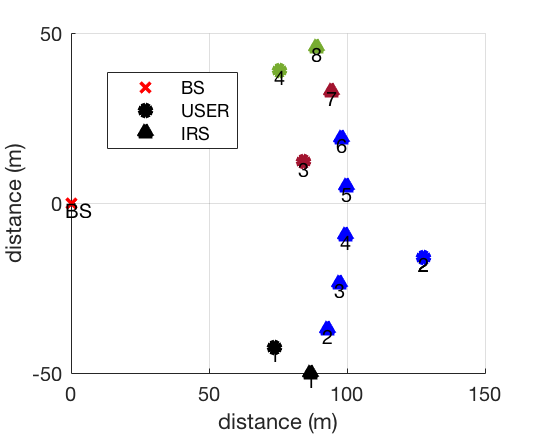
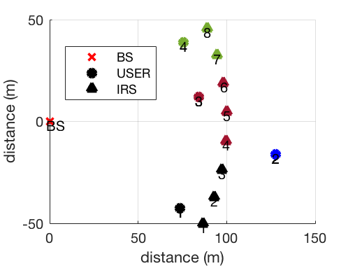
Figure 6: Association shown by color scheme. An IRS and a user are shown to be associated by having the same color.

Next we study how the users in Fig. 3(b) are associated with different IRSs under different IRS-user association methods. In Fig. 6(a), the associations are updated based on nearest rule, where each IRS is assigned to the user that has the shortest distance to it. On the other hand, Fig. 6(b) shows the IRS-user association resulting from the outlined SR Algorithm 1, which focuses on maximizing the SINR of the bottleneck user. It is clear from the deployment in Fig. 3(b) that user $2$ is the bottleneck user and we can see in Fig. 6(b) that SR algorithm managed to assign more IRSs to this user. We will see later in Fig. 8 that by doing so, the system achieves a higher minimum average SINR. Fig. 6(c) shows the result under exhaustive search IRS-user association. Again more IRSs are assigned to the second user is determined in the deployment to be the bottleneck user.

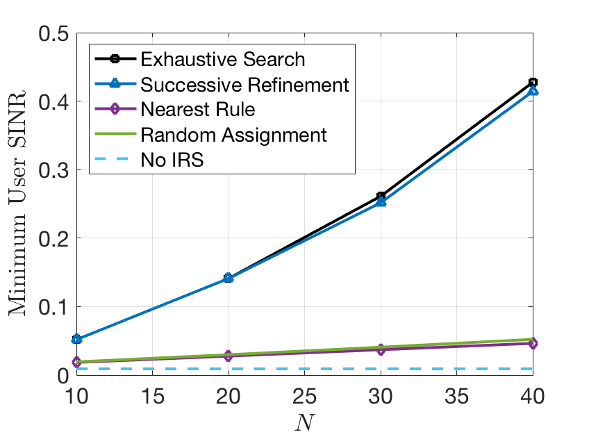
Figure 7: Minimum user SINR vs $N$.

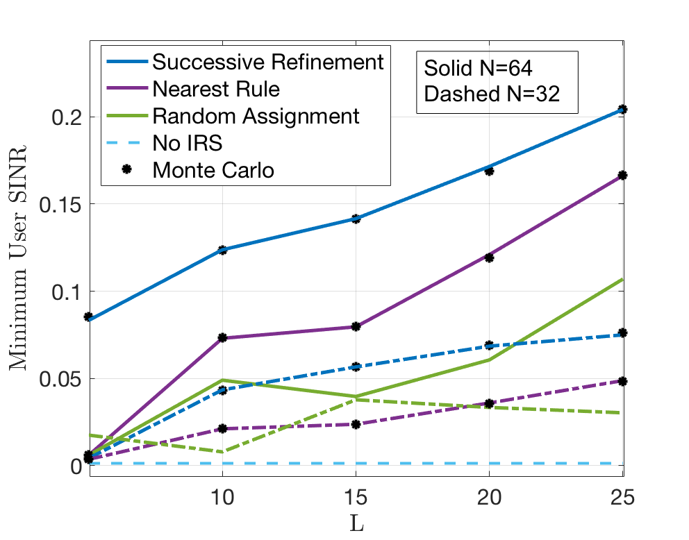
Figure 8: Minimum user SINR vs $L$.

Plotting the minimum user average SINR with average SINR derived in (45) against $N$ in Fig. 8, we notice that the SR algorithm explained in Algorithm 1 achieves a close performance to that of exhaustive search. Exhaustive search has complexity in the order of $\mathcal{O}(K^{L})$, and would therefore not scale well with the number of users and IRSs in the system. Hence the SR algorithm, which scales linearly with $L$, is an effective method to (nearly optimally) solve the IRS-user association problem. We also observe from Fig. 8 that the minimum user SINR improves with increasing the number of elements $N$ but not in the order of $N^{2}$. Generally for single user systems where there is no interference, deploying IRSs achieves gains in the order $N^{2}$ in the receiver’s SNR which is a combination of the array and passive beamforming gains [2], [31]. The reason we do not see an $N^{2}$ gain in multi-user systems is when we increase $N$ we not only increase the channel gain at the user but also the interference experienced.

Also note that the nearest distance rule and random assignment yield a much lower minimum average SINR, which is attributed to the fact that they do not necessarily help the bottleneck user. However, a distributed IRSs-assisted system with nearest distance rule and random IRS-user assignment does perform better than a system with no IRS because as we mentioned before, even the non-associated IRSs will contribute to the bottleneck user’s channel gain which is seen in Lemma 3 and the discussion underneath it.

Next we study the minimum average SINR against $L$ in Fig. 8. We plot the Monte-Carlo simulated average SINR in (28) as well as the derived expression (45) for the average SINR in Theorem 1. The Monte-Carlo simulated values are averaged over 1000 channel realizations and are shown to match the theoretical expression accurately thereby validating Theorem 1. Since exhaustive search does not scale well with increasing $L$, we did not include it in this plot. However, it has already been established in the previous figure that the solution yielded by SR performs very close to that yielded by exhaustive search which is optimal. Increasing the number of IRSs is beneficial as expected, since there are more IRSs to be assigned to the users resulting in higher, passive beamforming gains. The solid lines in the figure represent a doubled number of IRS elements than that represented by the dashed lines. We can see that doubling $N$ improves the minimum user SINR as expected. Moreover, we see that nearest distance rule assignment increases the minimum user SINR but at a slower rate than SR. Meanwhile, random assignment may increase the minimum user SINR or not as depicted, since the IRSs can be associated randomly in a detrimental manner to the minimum user SINR.

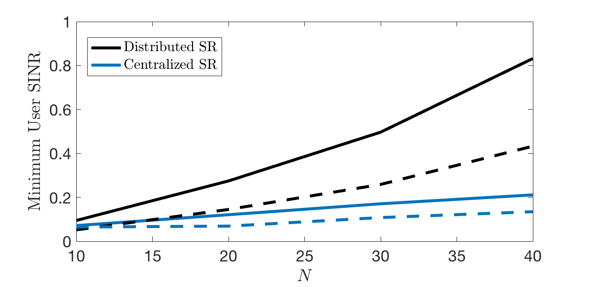
Figure 9: Minimum user SINR against $N$ under centralized and distributed IRSs deployment scenarios. Solid lines represent $L=16$, dashed lines represent $L=8$.

Fig. 9 depicts the minimum user SINR when the IRSs are distributed as opposed to having the IRSs as one central unit. Centralized deployment of IRSs compacts the $L$ IRSs, which can be effectively represented by a single large IRS with $NL$ elements. Distributed IRSs assisted system performs better than the centralized IRS assisted system because of the spatial diversity that the distributed placement offers. Especially under LoS BS-IRS propagation, the BS-IRS channel is almost certain to be rank-deficient since the IRS is in the far-field of the BS, which lessens the degrees of freedom offered by the channel. Having the IRSs distributed increases the degrees of freedom to at least $L$, resulting in better minimum SINR performance.

(a)

(b)

Figure 10: IRSs-users association patterns under distributed and centralized deployments.

Next we study the way the users are associated with the IRSs when the IRSs are distributed versus when all IRSs are located together. Considering $L=16$, we plot in Fig. 10(a) and Fig. 10(b) the SR optimized association for the distributed and centralized IRSs scenarios respectively. One can see that when IRSs are located together, almost all the users have a larger distance to the centralized IRSs and will experience higher path loss resulting in the SR algorithm to balance the IRSs between all users. Whereas in the distributed case, the IRSs are better distributed to cover all users and the SR algorithm will assign most IRSs to the bottleneck user (user $2$). The lack of nearby IRSs to all users has an adverse impact on the system performance, and the minimum user SINR deteriorates under the centralized deployment.

VI Conclusion

The work considered a distributed IRSs assisted multi-user MISO system, where the IRSs are associated with users in an optimized manner. We derived a tractable average SINR expression using statistical tools under MRT precoding, optimized IRS reflect beamforming, and arbitrary IRS-user association parameters. The expression was used to formulate and solve a max-min average SINR problem to optimize the IRS-user association parameters using a low-complexity SR algorithm. Simulation results validated the average SINR expression and studied the effect of increasing the number of IRSs, the number of elements in each IRS, as well as changing the physical distribution of the IRSs and IRS-user association pattern. In particular, the results show that that the minimum user SINR gets quadrupled when the IRSs are deployed in a distributed manner as opposed to centralized manner. The sub-optimal SR algorithm is shown to perform closely to the optimal solution given by exhaustive search. An important future direction will be to extend the theoretical analysis for average SINR to imperfect CSI scenario as well as multi-cell systems.

Appendix A Proof of Lemma 3

We wish to show the expectation of the squared norm of the channel given as

$$\mathbb{E}[\|{\mathbf{h}}_{k}(\boldsymbol{\lambda_{k}})\|^{2}]=E_{1}+E_{2}+E_{3}+E_{4}+E_{5}+E_{6},$$ (52)

$$\text{where, }\hskip 7.22743ptE_{1}=\mathbb{E}[\mathbf{h}_{d,k}^{H}\mathbf{h}_{d,k}]=M\beta_{d,k},$$ (53)

$$E_{2}=\mathbb{E}[2\sum_{l=1}^{L}\lambda_{l,k}\mathbf{v}_{l}^{{k_{l}}^{H}}\mathbf{H}_{0,l,k}^{H}\mathbf{h}_{d,k}],$$ (54)

$$E_{3}=\mathbb{E}[\sum_{l=1}^{L}\sum_{\bar{l}=1}^{L}\lambda_{l,k}\lambda_{\bar{l},k}\mathbf{v}_{l}^{{k_{l}}^{H}}\mathbf{H}_{0,l,k}^{H}\mathbf{H}_{0,\bar{l},k}\mathbf{v}_{\bar{l}}^{{k_{\bar{l}}}}],$$ (55)

$$E_{4}=\mathbb{E}[\sum_{l=1}^{L}\sum_{\bar{l}=1}^{L}(1-\lambda_{l,k})(1-\lambda_{\bar{l},k})\mathbf{v}_{l}^{k_{l}^{H}}\mathbf{H}_{0,l,k}^{H}\mathbf{H}_{0,\bar{l},k}\mathbf{v}_{\bar{l}}^{{k_{\bar{l}}}}],$$ (56)

$$E_{5}=\mathbb{E}[2\sum_{l=1}^{L}(1-\lambda_{l,k})\mathbf{v}_{l}^{k_{l}^{H}}\mathbf{H}_{0,l,k}^{H}\mathbf{h}_{d,k}],$$ (57)

$$E_{6}=\mathbb{E}[2\sum_{l=1}^{L}\sum_{\bar{l}=1}^{L}(1-\lambda_{\bar{l},k})\lambda_{{l},k}\mathbf{v}_{l}^{{k_{l}}^{H}}\mathbf{H}_{0,l,k}^{H}\mathbf{H}_{0,\bar{l},k}\mathbf{v}_{\bar{l}}^{{k_{\bar{l}}}}],$$ (58)

where $\mathbf{v}_{l}^{k_{l}}$ defined in (24) and ${\mathbf{h}}_{k}(\boldsymbol{\lambda}_{k})$ defined in (18). First we work on $E_{2}$, which is the inner product of the cascaded IRS channel and the direct channel with the optimized IRS configuration $\mathbf{v}_{l}^{k_{l}}$ where $k_{l}=k$. We obtain

$$E_{2}=2\sum_{l=1}^{L}\lambda_{l,k}\mathbb{E}[\mathbf{v}_{l}^{{k_{l}}^{H}}\mathbf{H}_{0,l,k}^{H}\mathbf{h}_{d,k}]=2\sum_{l=1}^{L}\lambda_{l,k}\mathbb{E}[\sum_{n=1}^{N}e^{j\angle{{h}_{2,l,k,n}{b}_{l,n}^{*}}}e^{j\angle{\mathbf{h}_{d,k}^{H}\mathbf{a}_{l}}}{h}_{2,l,k,n}^{*}{b}_{l,n}\mathbf{a}_{l}^{H}\mathbf{h}_{d,k}]$$ (59)

$$=2\sum_{l=1}^{L}\lambda_{l,k}\mathbb{E}[\sum_{n=1}^{N}e^{j(\angle{{h}_{2,l,k,n}{b}_{l,n}^{*}}-\angle{{h}_{2,l,k,n}{b}_{l,n}^{*}})}e^{j(\angle{\mathbf{h}_{d,k}^{H}\mathbf{a}_{l}}-\angle{\mathbf{h}_{d,k}^{H}\mathbf{a}_{l}})}|{h}_{2,l,k,n}^{*}{b}_{l,n}||\mathbf{a}_{l}^{H}\mathbf{h}_{d,k}|]$$ (60)

$$=2\sqrt{\beta_{1,l}}\sum_{l=1}^{L}\lambda_{l,k}\mathbb{E}[\sum_{n=1}^{N}|{h}_{2,l,k,n}|\cdot|\mathbf{a}_{l}^{H}\mathbf{h}_{d,k}|]=2\sqrt{\beta_{1,l}\beta_{d,k}\beta_{2,l,k}}\sum_{l=1}^{L}\lambda_{l,k}\sum_{n=1}^{N}\frac{\pi}{4}\sqrt{\mathbf{a}_{l}^{H}\mathbf{a}_{l}}$$ (61)

$$=2\sqrt{\beta_{1,l}\beta_{d,k}\beta_{2,l,k}}\sum_{l=1}^{L}\lambda_{l,k}\frac{\pi}{4}\sqrt{M}N,$$ (62)

where $\mathbf{H}_{0,l,k}$ is given in (16), ${h}_{2,l,k}(n)$ is the $n^{th}$ element in $\mathbf{h}_{2,l,k}$, and (61) follows since $|{h}_{2,l,k}(n)|$ and $|\mathbf{a}_{l}^{H}\mathbf{h}_{d,k}|$ are statistically independent Rayleigh distributed random variables whose mean values are given as $\sqrt{\pi\beta_{2,l,k}}/2$ and $\sqrt{\pi\beta_{dk}\mathbf{a}_{l}^{H}\mathbf{a}_{l}}/2$, respectively.

Next we work on $E_{3}$ where $k_{l}=k$ as follows

$$E_{3}=\mathbb{E}[\sum_{l=1}^{L}\sum_{\bar{l}=1}^{L}\lambda_{l,k}\lambda_{\bar{l},k}\mathbf{v}_{l}^{{k_{l}}^{H}}\mathbf{H}_{0,l,k}^{H}\mathbf{H}_{0,\bar{l},k}\mathbf{v}_{\bar{l}}^{{k_{\bar{l}}}}]$$ (63)

$$=\sum_{l=1}^{L}\lambda_{l,k}\mathbb{E}[\mathbf{v}_{l}^{{k_{l}}^{H}}\mathbf{H}_{0,l,k}^{H}\mathbf{H}_{0,{l},k}\mathbf{v}_{l}^{k_{l}}]+\sum_{l=1}^{L}\sum_{\bar{l}\neq l}^{L}\lambda_{l,k}\lambda_{\bar{l},k}\mathbb{E}[\mathbf{v}_{l}^{{k_{l}}^{H}}\mathbf{H}_{0,l,k}^{H}\mathbf{H}_{0,\bar{l},k}\mathbf{v}_{\bar{l}}^{{k_{\bar{l}}}}]$$ (64)

$$=\sum_{l=1}^{L}\lambda_{l,k}\mathbb{E}[\|\mathbf{H}_{0,{l},k}\mathbf{v}_{l}^{k_{l}}\|^{2}],$$ (65)

where the term with the sum $l\neq\bar{l}$ is zero due to independence between the different $\mathbf{h}_{2,l,k}$, $l=1,\dots,L$. Now, we can use a result for CGQF [32] to obtain

$$E_{3} =\sum_{l=1}^{L}\lambda_{l,k}\mathbb{E}[\mathbf{e}^{j\angle\mathbf{h}_{d,k}^{H}\mathbf{H}_{0,l,k}}\mathbf{H}_{0,l,k}^{H}\mathbf{H}_{0,{l},k}\mathbf{e}^{j\angle\mathbf{H}_{0,l,k}^{H}\mathbf{h}_{d,k}}]=\sum_{l=1}^{L}\lambda_{l,k}\mathbb{E}[\tilde{\mathbf{v}}_{l}^{{k_{l}}^{H}}\mathbf{A}\tilde{\mathbf{v}}_{l}^{{k_{l}}}],$$ (66)

where $\tilde{\mathbf{v}}_{l}^{{k_{l}}}=\text{diag}(|\mathbf{h}_{2,l,k}|)\mathbf{e}^{j\angle\mathbf{H}_{1,l}^{H}\mathbf{h}_{d,k}}$, and

$$\mathbf{A}=\mathbf{H}_{1,l}^{H}\mathbf{H}_{1,{l}}=\beta_{1,l}\|\mathbf{a}_{l}\|^{2}\mathbf{b}_{l}\mathbf{b}_{l}^{H}$$ (67)

is a symmetric, deterministic matrix. We can now write

$$E_{3} =\sum_{l=1}^{L}\lambda_{l,k}\mathbb{E}[\tilde{\mathbf{v}}_{l}^{{k_{l}}^{H}}\mathbf{A}\tilde{\mathbf{v}}_{l}^{{k_{l}}}]=\sum_{l=1}^{L}\lambda_{l,k}\big{(}tr(\mathbf{A}\boldsymbol{\Sigma}_{\tilde{\mathbf{v}}_{l}^{{k_{l}}}})+\boldsymbol{\mu}_{\tilde{\mathbf{v}}_{l}^{{k_{l}}}}^{H}\mathbf{A}\boldsymbol{\mu}_{\tilde{\mathbf{v}}_{l}^{{k_{l}}}}\big{)},$$ (68)

where $\boldsymbol{\Sigma}_{\tilde{\mathbf{v}}_{l}^{{k_{l}}}}=\mathbb{E}[\tilde{\mathbf{v}}_{l}^{{k_{l}}}\tilde{\mathbf{v}}_{l}^{{k_{l}}^{H}}]$ and $\mu_{\tilde{v}_{l}^{k}}=\mathbb{E}[\tilde{\mathbf{v}}_{l}^{{k_{l}}}]$. Next, we express $\boldsymbol{\Sigma}_{\tilde{\mathbf{v}}_{l}^{{k_{l}}}}$ using Lemma 7.

Lemma 7

The expectation of $\mathbf{D}\mathbf{A}\mathbf{D}$ where $\mathbf{D}\in\mathbb{C}^{S\times S}$ is a random diagonal matrix and $\mathbf{A}\in\mathbb{C}^{S\times S}$ is a symmetric, deterministic matrix is given by

$$\mathbb{E}[[\mathbf{D}\mathbf{A}\mathbf{D}]_{i,j}]=\mathbb{E}[\mathbf{d}_{i}^{T}\mathbf{A}_{i,j}\mathbf{d}_{j}],\forall i,j$$ (69)

where $\mathbf{d}_{i}$ is the $i^{th}$ column in $\mathbf{D}$ and

$$\mathbb{E}[\mathbf{d}_{i}^{T}\mathbf{A}_{i,i}\mathbf{d}_{i}]=\mathbb{E}[\mathbf{d}_{i}^{T}\mathbf{d}_{i}]\mathbf{A}_{i,i}=\sum_{s=1}^{S}\mathbb{E}[{d}_{i,s}^{2}]\mathbf{A}_{i,i}=\sum_{s=1}^{S}(\text{Var}({d}_{i,s})+\mathbb{E}[{d}_{i,s}]^{2})\mathbf{A}_{i,i},$$ (70)

$$\mathbb{E}[\mathbf{d}_{i}^{T}\mathbf{A}_{i,j}\mathbf{d}_{j}]=\mathbb{E}[\mathbf{d}_{i}^{T}]\mathbf{A}_{i,j}\mathbb{E}[\mathbf{d}_{j}],\hskip 7.22743pti\neq j.$$ (71)

Using Lemma 7, the covariance matrix $\boldsymbol{\Sigma}_{\tilde{\mathbf{v}}_{l}^{{k_{l}}}}$ is found to be

$$\boldsymbol{\Sigma}_{\tilde{\mathbf{v}}_{l}^{{k_{l}}}}=\mathbb{E}[\tilde{\mathbf{v}}_{l}^{{k_{l}}}\tilde{\mathbf{v}}_{l}^{{k_{l}}^{H}}]=\mathbb{E}[\text{diag}(|\mathbf{h}_{2,l,k}|)\mathbf{e}^{j\angle\mathbf{H}_{1,l}^{H}\mathbf{h}_{d,k}}\mathbf{e}^{j\angle\mathbf{h}_{d,k}^{H}\mathbf{H}_{1,l}}\text{diag}(|\mathbf{h}_{2,l,k}|)]$$ (72)

$$=\mathbb{E}_{\mathbf{h}_{2,l,k}}[\text{diag}(|\mathbf{h}_{2,l,k}|)\mathbb{E}_{\mathbf{h}_{d,k}}[\mathbf{e}^{j\angle\mathbf{b}_{l}\mathbf{a}_{l}^{H}\mathbf{h}_{d,k}}\mathbf{e}^{j\angle\mathbf{h}_{d,k}^{H}\mathbf{a}_{l}\mathbf{b}_{l}^{H}}]\text{diag}(|\mathbf{h}_{2,l,k}|)]$$ (73)

$$=(1-\frac{\pi}{4}+\frac{\pi}{4})\beta_{2,l,k}\mathbf{e}^{j\angle\mathbf{H}_{1,l}^{H}\mathbf{H}_{1,l}}\odot\mathbf{I}_{N}+\frac{\pi\beta_{2,l,k}}{4}\mathbf{e}^{j\angle\mathbf{H}_{1,l}^{H}\mathbf{H}_{1,l}}\odot(\mathbf{1}_{N}-\mathbf{I}_{N}),$$ (74)

$$=\beta_{2,l,k}\mathbf{I}_{N}+\frac{\pi\beta_{2,l,k}}{4}\mathbf{e}^{j\angle\mathbf{H}_{1,l}^{H}\mathbf{H}_{1,l}}\odot(\mathbf{1}_{N}-\mathbf{I}_{N}),$$ (75)

In step (73), we recall the model of $\mathbf{H}_{1,l}$ in (7). Notice that (74) follows from Lemma 7 and using the definitions of mean and variance of a Rayleigh distributed random variable. Furthermore, $\boldsymbol{\mu}_{\tilde{\mathbf{v}}_{l}^{{k_{l}}}}$ is derived as $\boldsymbol{\mu}_{\tilde{\mathbf{v}}_{l}^{{k_{l}}}}=\mathbb{E}[\tilde{\mathbf{v}}_{l}^{{k_{l}}}]=\mathbb{E}[\text{diag}(|\mathbf{h}_{2,l,k}|)\mathbf{e}^{j\angle\mathbf{H}_{1,l}^{H}\mathbf{h}_{d,k}}]=\mathbb{E}[\text{diag}(|\mathbf{h}_{2,l,k}|)]\mathbb{E}[\mathbf{e}^{j\angle\mathbf{H}_{1,l}^{H}\mathbf{h}_{d,k}}]]=\mathbf{0}_{N\times 1}.$ This follows from the independence between the direct and IRS-user channels, and from the fact that the phase distribution of a circularly symmetric complex normal random variable is uniform leading to $\mathbb{E}[\tilde{\mathbf{v}}_{l}^{{k_{l}}}]=0$.

As for the fourth term, recall that $\mathbf{v}_{l}^{k_{l}}$ (24) in $E_{4}$ (56) is the beamforming vector of non-associated IRS $l$ with respect to user $k$ for which $k_{l}\neq k$ such that $\lambda_{l,k}=0$ and $\lambda_{l,k_{l}}=1$. Its covariance matrix $\boldsymbol{\Sigma}_{\mathbf{v}_{l}^{k_{l}}}=\mathbf{I}_{N}$ which can be seen as

$$\boldsymbol{\Sigma}_{\mathbf{v}_{l}^{k_{l}}} =\mathbb{E}[\mathbf{v}_{l}^{k_{l}}\mathbf{v}_{l}^{k_{l}^{H}}]=\mathbb{E}[e^{j\angle{\text{diag}(\mathbf{h}_{2,l,k_{l}}^{H})\mathbf{b}_{l}}}e^{j\angle{\mathbf{a}_{l}^{H}\mathbf{h}_{d,k_{l}}}}e^{j\angle{\mathbf{b}_{l}^{H}\text{diag}(\mathbf{h}_{2,l,k_{l}})}}e^{j\angle{\mathbf{h}_{d,k_{l}}^{H}\mathbf{a}_{l}}}]$$ (76)

$$=\mathbb{E}[e^{j\angle{\text{diag}(\mathbf{h}_{2,l,k_{l}}^{H})\mathbf{b}_{l}}}e^{j\angle{\mathbf{b}_{l}^{H}\text{diag}(\mathbf{h}_{2,l,k_{l}})}}]$$ (77)

If we look at each element in the matrix in (77), we find that the diagonal elements are all ones, and the off-diagonals are all zeros due to independence between ${h}_{2,l,k_{l},n}$ and ${h}_{2,l,k_{l},\bar{n}}$ when $n\neq\bar{n}$, so that

$$\mathbb{E}[[e^{j\angle{\text{diag}(\mathbf{h}_{2,l,k_{l}}^{H})\mathbf{b}_{l}}}e^{j\angle{\mathbf{b}_{l}^{H}\text{diag}(\mathbf{h}_{2,l,k_{l}})}}]_{n,\bar{n}}]=\mathbb{E}[e^{j(\angle{{h}_{2,l,k_{l},n}^{*}{b}_{l,n}}-\angle{{h}_{2,l,k_{l},\bar{n}}^{*}{b}_{l,\bar{n}}})}]=0.$$ (78)

Using the above $\boldsymbol{\Sigma}_{\mathbf{v}_{l}^{k_{l}}}=\mathbf{I}_{N}$, we obtain

$$E_{4} =\mathbb{E}[\sum_{l=1}^{L}\sum_{\bar{l}=1}^{L}(1-\lambda_{l,k})(1-\lambda_{\bar{l},k})\mathbf{v}_{l}^{k_{l}^{H}}\mathbf{H}_{0,l,k}^{H}\mathbf{H}_{0,\bar{l},k}\mathbf{v}_{\bar{l}}^{{k_{\bar{l}}}}],$$ (79)

$$=\sum_{l=1}^{L}(1-\lambda_{l,k})\mathbb{E}[\mathbf{v}_{l}^{k_{l}^{H}}\mathbf{H}_{0,l,k}^{H}\mathbf{H}_{0,{l},k}\mathbf{v}_{{l}}^{k_{l}}]=\sum_{l=1}^{L}(1-\lambda_{l,k})\beta_{2,l,k}tr(\mathbf{A}),$$ (80)

with $\mathbf{A}$ defined as in (67). Note that the derivation of (80) follows using similar steps as done for $E_{3}$ in (63). The fifth term $E_{5}$ is equal to zero due to the zero conditional expectation of $\mathbf{h}_{d,k}$ given $\mathbf{h}_{d,k_{l}},\mathbf{h}_{2,l,k_{l}},\mathbf{h}_{2,l,k}$ where $k_{l}\neq k$ as follows

$$E_{5} =2\sum_{l=1}^{L}(1-\lambda_{l,k})\mathbb{E}[\mathbf{v}_{l}^{k_{l}^{H}}\mathbf{H}_{0,l,k}^{H}\mathbb{E}[\mathbf{h}_{d,k}|\mathbf{h}_{d,k_{l}},\mathbf{h}_{2,l,k_{l}},\mathbf{h}_{2,l,k}]]=0$$ (81)

Finally, the sixth term $E_{6}$ is zero using similar arguments as $E_{5}$.

Appendix B Proof of Lemma 6

In Lemma 6, we defined $\mathbf{R}_{k}$ as the covariance matrix of $\mathbf{h}_{k}(\boldsymbol{\lambda}_{k})$. In this appendix, we derive this matrix. Note that

$$\mathbf{R}_{k}=\mathbf{R}_{k,1}+\mathbf{R}_{k,2}+\mathbf{R}_{k,3}+\mathbf{R}_{k,4}+\mathbf{R}_{k,5}+\mathbf{R}_{k,6},$$ (82)

where

$$\mathbf{R}_{k,1}=\mathbb{E}[\mathbf{h}_{d,k}\mathbf{h}_{d,k}^{H}]=\beta_{d,k}\mathbf{I}_{M},\hskip 14.45377pt\mathbf{R}_{k,2}=\mathbb{E}[2\sum_{l=1}^{L}\lambda_{l,k}\mathbf{h}_{d,k}\mathbf{v}_{l}^{{k_{l}}^{H}}\mathbf{H}_{0,l,k}^{H}],$$ (83)

$$\mathbf{R}_{k,3}=\mathbb{E}[\sum_{l=1}^{L}\sum_{\bar{l}=1}^{L}\lambda_{l,k}\lambda_{\bar{l},k}\mathbf{H}_{0,l,k}\mathbf{v}_{l}^{k_{l}}\mathbf{v}_{\bar{l}}^{{k_{\bar{l}}}^{H}}\mathbf{H}_{0,\bar{l},k}^{H}],$$ (84)

$$\mathbf{R}_{k,4}=\mathbb{E}[\sum_{l=1}^{L}\sum_{\bar{l}=1}^{L}(1-\lambda_{l,k})(1-\lambda_{\bar{l},k})\mathbf{H}_{0,l,k}\mathbf{v}_{l}^{k_{l}}\mathbf{v}_{\bar{l}}^{k_{\bar{l}}^{H}}\mathbf{H}_{0,\bar{l},k}^{H}],$$ (85)

$$\mathbf{R}_{k,5}=\mathbb{E}[2\sum_{l=1}^{L}(1-\lambda_{l,k})\mathbf{H}_{0,l,k}\mathbf{v}_{l}^{k_{l}}\mathbf{h}_{d,k}^{H}]=\mathbf{0}_{M\times M},$$ (86)

$$\mathbf{R}_{k,6}=\mathbb{E}[2\sum_{l=1}^{L}\sum_{\bar{l}=1}^{L}(1-\lambda_{\bar{l},k})\lambda_{{l},k}\mathbf{H}_{0,\bar{l},k}\mathbf{v}_{\bar{l}}^{{k_{\bar{l}}}}\mathbf{v}_{l}^{{k_{l}}^{H}}\mathbf{H}_{0,l,k}^{H}]=\mathbf{0}_{M\times M},.$$ (87)

In appendix A, we show that $\mathbf{R}_{k,5}$ and $\mathbf{R}_{k,6}$ are zero matrices. To compute $\mathbf{R}_{k,2}$, we use the definition of $\mathbf{H}_{0,l,k}^{H}$ in (16) to write

$$\mathbf{R}_{k,2}= \mathbb{E}[2\sum_{l=1}^{L}\lambda_{l,k}\mathbf{h}_{d,k}\mathbf{v}_{l}^{{k_{l}}^{H}}\sqrt{\beta_{1,l}}\text{diag}(\mathbf{h}_{2,l,k}^{H})\mathbf{b}_{l}\mathbf{a}_{l}^{H}].$$ (88)

Its element form can be written as follows

$$[{\mathbf{R}}_{k,2}]_{m,\bar{m}}= 2\sqrt{\beta_{1,l}}\sum_{l=1}^{L}\lambda_{l,k}\mathbb{E}[h_{d,k,m}\mathbf{v}_{l}^{{k_{l}}^{H}}\text{diag}(\mathbf{h}_{2,l,k}^{H})\mathbf{b}_{l}{a}_{l,\bar{m}}^{*}],$$ (89)

where ${a}_{l,\bar{m}}^{*}$ is the $\bar{m}^{th}$ element in $\mathbf{a}_{l}^{H}$ and $h_{d,k,m}$ is the ${m}^{th}$ element in $\mathbf{h}_{d,k}$. We can further simplify by using the optimized reflection vector in (24) where $k_{l}=k$ to obtain

$$[{\mathbf{R}}_{k,2}]_{m,\bar{m}}= 2\sqrt{\beta_{1,l}}\sum_{l=1}^{L}\lambda_{l,k}\mathbb{E}[{h}_{d,k,m}\sum_{n=1}^{N}e^{j\angle{\mathbf{h}_{d,k}^{H}\mathbf{a}_{l}}}e^{j\angle{b_{l,n}^{*}{h}_{2,l,k,n}}}{h}_{2,l,k,n}^{*}{b}_{l,n}{a}_{l,\bar{m}}^{*}].$$ (90)

Here, ${h}_{2,l,k,n}$ is the ${n}^{th}$ element in $\mathbf{h}_{2,l,k}$, and ${b}_{l,n}$ is the ${n}^{th}$ element in $\mathbf{b}_{l}$. Thus, the phases cancel to yield

$$[{\mathbf{R}}_{k,2}]_{m,\bar{m}}= 2\sqrt{\beta_{1,l}}\sum_{l=1}^{L}\lambda_{l,k}\sum_{n=1}^{N}\sqrt{\frac{\pi\beta_{2,l,k}}{4}}{a}_{l,\bar{m}}^{*}\mathbb{E}\left[{h}_{d,k,m}e^{j\angle{\mathbf{h}_{d,k}^{H}\mathbf{a}_{l}}}\right]$$ (91)

$$=2\sqrt{\beta_{1,l}}\sum_{l=1}^{L}\lambda_{l,k}\sum_{n=1}^{N}\sqrt{\frac{\pi\beta_{2,l,k}}{4}}e^{j\angle{{a}_{l,\bar{m}}^{*}{a}_{l,m}}}\mathbb{E}\left[|{h}_{d,k,m}|e^{j\angle{(1+\frac{\sum_{i\neq m}^{M}{h}_{d,k,i}^{*}{a}_{l,i})}{{h}_{d,k,m}^{*}{a}_{l,m}})}}\right]$$ (92)

$$=2\sqrt{\beta_{1,l}}N\sum_{l=1}^{L}\lambda_{l,k}\sqrt{\frac{\pi\beta_{2,l,k}}{4}}e^{j\angle{{a}_{l,\bar{m}}^{*}{a}_{l,m}}}C_{m},$$ (93)

where $C_{m}=\mathbb{E}[|{h}_{d,k,m}|e^{j\angle{(1+\frac{\sum_{i\neq m}^{M}{h}_{d,k,i}^{*}{a}_{l,i})}{{h}_{d,k,m}^{*}{a}_{l,m}})}}]=\sqrt{\frac{\pi\beta_{d,k}}{4M}}$ by noting that $E_{2}=tr(\mathbf{R}_{k,2})$ where $E_{2}$ is defined in (62). Therefore we obtain

$$[\mathbf{R}_{k,2}]_{m,\bar{m}}= 2\sum_{l=1}^{L}\lambda_{l,k}\sqrt{\beta_{1,l}\beta_{2,l,k}\beta_{d,k}}N{\frac{\pi}{4\sqrt{M}}}e^{j\angle{{a}_{l,\bar{m}}^{*}{a}_{l,m}}}.$$ (94)

To compute $\mathbf{R}_{k,3}$, we have $k_{l}=k$ and we express it as

$$\mathbf{R}_{k,3} =\mathbb{E}[\sum_{l=1}^{L}\sum_{\bar{l}=1}^{L}\lambda_{l,k}\lambda_{\bar{l},k}\mathbf{H}_{0,l,k}\mathbf{v}_{l}^{k_{l}}\mathbf{v}_{\bar{l}}^{{k_{\bar{l}}}^{H}}\mathbf{H}_{0,\bar{l},k}^{H}]=\sum_{l=1}^{L}\lambda_{l,k}\mathbb{E}[\mathbf{H}_{0,l,k}\mathbf{v}_{l}^{k_{l}}\mathbf{v}_{l}^{{k_{l}}^{H}}\mathbf{H}_{0,{l},k}^{H}]$$ (95)

$$=\sum_{l=1}^{L}\lambda_{l,k}{\beta_{1,l}}\mathbf{H}_{1,l}\mathbb{E}[\text{diag}(|\mathbf{h}_{2,l,k}|)\mathbf{e}^{j\angle\mathbf{H}_{1,l}^{H}\mathbf{h}_{d,k}}\mathbf{e}^{j\angle\mathbf{h}_{d,k}^{H}\mathbf{H}_{1,l}}\text{diag}(|\mathbf{h}_{2,l,k}^{H}|)]\mathbf{H}_{1,l}^{H}$$ (96)

$$=\sum_{l=1}^{L}\lambda_{l,k}{\beta_{1,l}}\mathbf{H}_{1,l}\boldsymbol{\Sigma}_{\tilde{\mathbf{v}}_{l}^{{k_{l}}}}\mathbf{H}_{1,l}^{H}$$ (97)

The summation in (95) reduces due to independence between the different IRS-users channels. The last equivalence (97) is obtained following the result for $\boldsymbol{\Sigma}_{\tilde{\mathbf{v}}_{l}^{k_{l}}}$ defined in (72). Finally,

$$\mathbf{R}_{k,4} =\mathbb{E}[\sum_{l=1}^{L}\sum_{\bar{l}=1}^{L}(1-\lambda_{l,k})(1-\lambda_{\bar{l},k})\mathbf{H}_{0,l,k}\mathbf{v}_{l}^{k_{l}}\mathbf{v}_{\bar{l}}^{k_{\bar{l}}^{H}}\mathbf{H}_{0,\bar{l},k}^{H}]$$ (98)

$$=\sum_{l=1}^{L}\beta_{1,l}(1-\lambda_{l,k})\mathbb{E}[\mathbf{a}_{l}\mathbf{b}_{l}^{H}\text{diag}(\mathbf{h}_{2,l,k})\mathbf{v}_{l}^{k_{l}}\mathbf{v}_{l}^{k_{l}^{H}}\text{diag}(\mathbf{h}_{2,l,k}^{H})\mathbf{b}_{l}\mathbf{a}_{l}^{H}]=\sum_{l=1}^{L}\beta_{1,l}(1-\lambda_{l,k})\tilde{\mathbf{R}}_{k,4}$$ (99)

The summation reduces due to independence between the different IRS-users channels. Using $\mathbf{v}_{l}^{k_{l}}$ in (24), for $k_{l}\neq k$ and defining $\tilde{\mathbf{R}}_{k,4}$ we get

$$\tilde{\mathbf{R}}_{k,4} =\mathbb{E}[\mathbf{a}_{l}\mathbf{b}_{l}^{H}\text{diag}(\mathbf{h}_{2,l,k})e^{j\angle{\text{diag}(\mathbf{h}^{H}_{2,l,k_{l}})\mathbf{b}_{l}}}e^{j\angle{\mathbf{b}_{l}}^{H}\text{diag}(\mathbf{h}_{2,l,k_{l}})}\text{diag}(\mathbf{h}_{2,l,k}^{H})\mathbf{b}_{l}\mathbf{a}_{l}^{H}]$$ (100)

$$=\mathbf{a}_{l}\mathbf{b}_{l}^{H}\mathbb{E}_{\mathbf{h}_{2,l,k}}[\mathbb{E}[\text{diag}(\mathbf{h}_{2,l,k})e^{j\angle{\text{diag}(\mathbf{h}^{H}_{2,l,k_{l}})\mathbf{b}_{l}}}e^{j\angle{\mathbf{b}_{l}}^{H}\text{diag}(\mathbf{h}_{2,l,k_{l}})}\text{diag}(\mathbf{h}_{2,l,k}^{H})|\mathbf{h}_{2,l,k_{l}}]]\mathbf{b}_{l}\mathbf{a}_{l}^{H},$$ (101)

$$=\beta_{2,l,k}\|\mathbf{b}_{l}\|^{2}\mathbf{a}_{l}\mathbf{a}_{l}^{H}.$$ (102)

Notice that $\mathbb{E}[\text{diag}(\mathbf{h}_{2,l,k})e^{j\angle{\text{diag}(\mathbf{h}^{H}_{2,l,k_{l}})\mathbf{b}_{l}}}e^{j\angle{\mathbf{b}_{l}}^{H}\text{diag}(\mathbf{h}_{2,l,k_{l}})}\text{diag}(\mathbf{h}_{2,l,k}^{H})|\mathbf{h}_{2,l,k}]$ can be seen as random diagonal matrix $\text{diag}(\mathbf{h}^{H}_{2,l,k})$ multiplied by a deterministic matrix $e^{j\angle{\text{diag}(\mathbf{h}^{H}_{2,l,k_{l}})\mathbf{b}_{l}}}e^{j\angle{\mathbf{b}_{l}}^{H}\text{diag}(\mathbf{h}_{2,l,k_{l}})}$ multiplied by the same diagonal matrix. Therefore, we have the right set-up to apply Lemma 7 and get the following: the off-diagonals are equal to zero, while the diagonal terms are equal to $\beta_{2,l,k}$. Thus, we achieve a scaled identity for this expectation term which simplifies our expression when plugging $\tilde{\mathbf{R}}_{k,4}$ for $\mathbf{R}_{k,4}$ to obtain

$$\mathbf{R}_{k,4} =\sum_{l=1}^{L}(1-\lambda_{l,k})\beta_{1,l}\beta_{2,l,k}\|\mathbf{b}_{l}\|^{2}\mathbf{a}_{l}\mathbf{a}_{l}^{H}=\sum_{l=1}^{L}(1-\lambda_{l,k}){\beta_{2,l,k}}\mathbf{H}_{1,l}\mathbf{H}_{1,{l}}^{H}$$ (103)

Thus, we have completed the proof for Lemma 6.

References

• [1] M. Di Renzo, A. Zappone, M. Debbah, M. S. Alouini, C. Yuen, J. de Rosny, and S. Tretyakov, “Smart radio environments empowered by reconfigurable intelligent surfaces: How it works, state of research, and the road ahead,” IEEE Journal on Selected Areas in Communications, vol. 38, no. 11, pp. 2450–2525, 2020.
• [2] Q. Nadeem, A. Kammoun, A. Chaaban, M. Debbah, and M. Alouini, “Asymptotic max-min sinr analysis of reconfigurable intelligent surface assisted miso systems,” IEEE Trans. Wireless Commun., pp. 1–1, 2020.
• [3] S. Abeywickrama, R. Zhang, Q. Wu, and C. Yuen, “Intelligent reflecting surface: Practical phase shift model and beamforming optimization,” IEEE Transactions on Communications, vol. 68, no. 9, pp. 5849–5863, 2020.
• [4] J. He, K. Yu, and Y. Shi, “Coordinated passive beamforming for distributed intelligent reflecting surfaces network,” in 2020 IEEE 91st Vehicular Technology Conference (VTC2020-Spring), 2020, pp. 1–5.
• [5] Q. Wu and R. Zhang, “Intelligent reflecting surface enhanced wireless network via joint active and passive beamforming,” IEEE Transactions on Wireless Communications, vol. 18, no. 11, pp. 5394–5409, 2019.
• [6] X. Lu, E. Hossain, T. Shafique, S. Feng, H. Jiang, and D. Niyato, “Intelligent reflecting surface enabled covert communications in wireless networks,” IEEE Network, vol. 34, no. 5, pp. 148–155, 2020.
• [7] Y. Yang, B. Zheng, S. Zhang, and R. Zhang, “Intelligent reflecting surface meets ofdm: Protocol design and rate maximization,” IEEE Transactions on Communications, vol. 68, no. 7, pp. 4522–4535, 2020.
• [8] B. Zheng, C. You, and R. Zhang, “Intelligent reflecting surface assisted multi-user ofdma: Channel estimation and training design,” IEEE Transactions on Wireless Communications, vol. 19, no. 12, pp. 8315–8329, 2020.
• [9] Q. Wu and R. Zhang, “Weighted sum power maximization for intelligent reflecting surface aided swipt,” IEEE Wireless Communications Letters, vol. 9, no. 5, pp. 586–590, 2020.
• [10] Q. Wu and R. Zhang, “Joint active and passive beamforming optimization for intelligent reflecting surface assisted swipt under qos constraints,” IEEE Journal on Selected Areas in Communications, vol. 38, no. 8, pp. 1735–1748, 2020.
• [11] M. A. Kishk and M.-S. Alouini, “Exploiting Randomly-located Blockages for Large-Scale Deployment of Intelligent Surfaces,” arXiv e-prints, p. arXiv:2001.10766, Jan. 2020.
• [12] J. He, K. Yu, and Y. Shi, “Coordinated Passive Beamforming for Distributed Intelligent Reflecting Surfaces Network,” arXiv e-prints, p. arXiv:2002.05915, Feb. 2020.
• [13] Q.-U.-A. Nadeem, A. Kammoun, A. Chaaban, M. Debbah, and M.-S. Alouini, “Intelligent reflecting surface assisted wireless communication: Modeling and channel estimation,” 2019.
• [14] W. Mei and R. Zhang, “Performance analysis and user association optimization for wireless network aided by multiple intelligent reflecting surfaces,” 2020.
• [15] A. Epstein and G. V. Eleftheriades, “Synthesis of passive lossless metasurfaces using auxiliary fields for reflectionless beam splitting and perfect reflection,” Phys. Rev. Lett., vol. 117, p. 256103, Dec 2016. [Online]. Available: https://link.aps.org/doi/10.1103/PhysRevLett.117.256103
• [16] F. Rusek, D. Persson et al., “Scaling up MIMO: Opportunities and challenges with very large arrays,” IEEE Signal Processing Magazine, vol. 30, no. 1, pp. 40–60, Jan. 2013.
• [17] Q.-U.-A. Nadeem, A. Kammoun, M. Debbah, and M.-S. Alouini, “Design of 5g full dimension massive mimo systems,” IEEE Transactions on Communications, vol. 66, no. 2, pp. 726–740, 2018.
• [18] E. Björnson, E. G. Larsson, and M. Debbah, “Massive mimo for maximal spectral efficiency: How many users and pilots should be allocated?” IEEE Transactions on Wireless Communications, vol. 15, no. 2, pp. 1293–1308, 2016.
• [19] H. Alwazani, Q.-U.-A. Nadeem, and A. Chaaban, “Channel estimation for distributed intelligent reflecting surfaces assisted multi-user miso systems,” 2020.
• [20] G. Zhou et al., “Robust beamforming design for intelligent reflecting surface aided miso communication systems,” IEEE Wireless Communications Letters, pp. 1–1, 2020.
• [21] Q.-U.-A. Nadeem et al., “Intelligent reflecting surface assisted multi-user miso communication: Channel estimation and beamforming design,” IEEE Open J. Commun. Soc., vol. PP, pp. 1–1, May 2020.
• [22] Z. Wan, Z. Gao, and M.-S. Alouini, “Broadband Channel Estimation for Intelligent Reflecting Surface Aided mmWave Massive MIMO Systems,” arXiv e-prints, p. arXiv:2002.01629, Feb. 2020.
• [23] Q. Wu and R. Zhang, “Intelligent reflecting surface enhanced wireless network: Joint active and passive beamforming design,” in 2018 IEEE Global Communications Conference (GLOBECOM), Dec 2018, pp. 1–6.
• [24] D. Tse and P. Viswanath, MIMO I: spatial multiplexing and channel modeling.   Cambridge University Press, 2005, p. 290–331.
• [25] I. Khaled, A. E. Falou, C. Langlais, B. E. Hassan, and M. Jezequel, “Multi-User Digital Beamforming Based on Path Angle Information for mm-Wave MIMO Systems,” in WSA 2020 : 24th International ITG Workshop on Smart Antennas, Hambourg, Germany, Feb. 2020. [Online]. Available: https://hal.archives-ouvertes.fr/hal-02474863
• [26] X. Li, J. Fang, F. Gao, and H. Li, “Joint active and passive beamforming for intelligent reflecting surface-assisted massive mimo systems,” ArXiv, vol. abs/1912.00728, 2019.
• [27] H. Tataria, P. J. Smith, A. F. Molisch, S. Sangodoyin, M. Matthaiou, P. A. Dmochowski, J. Zhang, and R. S. Thoma, “Spatial correlation variability in multiuser systems,” in 2018 IEEE International Conference on Communications (ICC), 2018, pp. 1–7.
• [28] L. Yu, W. Liu, and R. Langley, “Sinr analysis of the subtraction-based smi beamformer,” IEEE Transactions on Signal Processing, vol. 58, no. 11, pp. 5926–5932, 2010.
• [29] P. Ramirez Espinosa et al., “Analysis of gaussian quadratic forms with application to statistical channel modeling,” 2020.
• [30] E. Björnson, J. Hoydis, and L. Sanguinetti, “Massive MIMO networks: Spectral, energy, and hardware efficiency,” Foundations and Trends® in Signal Processing, vol. 11, no. 3-4, pp. 154–655, 2017. [Online]. Available: http://dx.doi.org/10.1561/2000000093
• [31] E. Björnson, . Özdogan, and E. G. Larsson, “Reconfigurable intelligent surfaces: Three and two critical questions,” IEEE Communications Magazine, vol. 58, no. 12, pp. 90–96, 2020.
• [32] A. Mathai and S. Provost, Quadratic Forms in Random Variables: Theory and Applications, 12 1992, vol. 87.