Accelerated replica exchange stochastic gradient Langevin diffusion enhanced Bayesian DeepONet for solving noisy parametric PDEs
Abstract
The Deep Operator Networks (DeepONet) is a fundamentally different class of neural networks that we train to approximate nonlinear operators, including the solution operator of parametric partial differential equations (PDE). DeepONets have shown remarkable approximation and generalization capabilities even when trained with relatively small datasets. However, the performance of DeepONets deteriorates when the training data is polluted with noise, a scenario that occurs very often in practice. To enable DeepONets training with noisy data, we propose using the Bayesian framework of replica-exchange Langevin diffusion. Such a framework uses two particles, one for exploring and another for exploiting the loss function landscape of DeepONets. We show that the proposed framework’s exploration and exploitation capabilities enable (1) improved training convergence for DeepONets in noisy scenarios and (2) attaching an uncertainty estimate for the predicted solutions of parametric PDEs. In addition, we show that replica-exchange Langeving Diffusion (remarkably) also improves the DeepONet’s mean prediction accuracy in noisy scenarios compared with vanilla DeepONets trained with state-of-the-art gradient-based optimization algorithms (e.g., Adam). To reduce the potentially high computational cost of replica, in this work, we propose an accelerated training framework for replica-exchange Langevin diffusion that exploits the neural network architecture of DeepONets to reduce its computational cost up to 25% without compromising the proposed framework’s performance. Finally, we illustrate the effectiveness of the proposed Bayesian framework using a series of experiments on four parametric PDE problems.
1 Introduction
Many problems in Science and Engineering require solving parametric PDEs [1, 19, 16, 29]. That is, they require the repeated evaluation of a PDE model for a given distribution of inputs. For example, in petroleum engineering applications, engineers seek to calculate, using the porous media equations, the pressure field of the oil based on its permeability. In practice, the value of the oil permeability varies frequently; hence, one needs to calculate the oil pressure field for a distribution of fast-varying permeabilities [29, 9, 11]. The traditional numerical frameworks require intense computations to solve these parametric PDEs. Furthermore, the computational cost for these traditional frameworks increases even more when the problem is time-dependent and multiscale [10, 6, 15].
To reduce the computational cost for solving parametric PDEs, many works have proposed using deep neural networks, which transfer most of the cost to offline training. However, the data required to train these networks is often polluted with noise or numerical errors in practice. In these noisy scenarios, deep neural networks often have poor generalization performance because the gradient-based algorithms used to train the networks tend to chase the noise. As a result, the trained model will fail if used in practice.
This work focuses on Deep Operator Networks (DeepONet) [25], a fundamentally different class of neural networks that learns to approximate nonlinear operators, i.e., mappings between infinite-dimensional function spaces. DeepONets are constructed to realize and exploit the power of the universal approximation theorem of operators [3]. To that end, a DeepONet uses two sub-networks: one is called the Branch net, which encodes the input function at a fixed number of locations; and another one is called the Trunk net, which encodes the locations where one evaluates the output function. Such an architecture enables DeepONets to learn nonlinear operators efficiently from relatively small datasets. The remarkable capabilities of DeepONets have been reported in many application areas, including electroconvection [2], chemistry [23], economics [22], and for solving parametric PDEs [25]. These previous works, however, have only trained DeepONets using data without noise. In real applications, data is often polluted with noise. So, a framework that can handle noisy data during DeepONets’ training must be developed.
Many works have studied the problem of dealing with noisy datasets and avoiding overfitting. Among these works, Bayesian frameworks [26] that use the Langevin diffusion [26, 4] have provided promising results. For example, in [26], the authors introduced the Stochastic Gradient Langevin diffusion algorithm to train neural networks. They demonstrated that the samples generated by their proposed algorithm converge to the target posterior distribution. Replica-exchange MCMC and (its stochastic gradient variants) were proposed [24, 5, 12] to accelerate the Langevin diffusion. In replica-exchange frameworks, instead of using one particle to sample from the posterior, one uses two particles with different temperature parameters. The high-temperature particle explores the landscape of the loss function, which enables escaping from local minima, while the low temperature exploits the same landscape, enforcing local convergence [18, 28]. The two particles can be exchanged according to a swapping probability. If this swapping probability is designed so that the Markov process is reversible, then the low-temperature particle may attain the global optima faster.
Replica-exchange frameworks provide us with excellent convergence performance. They, however, double the computational on each training iteration. Hence, one needs to balance having fast convergence (i.e., fewer iteration steps) and haven high per-iteration computational cost. To tackle such a problem, in our previous work [24], we proposed the multi-variance stochastic gradient Langevin diffusion (m-reSGLD) framework, which assumes that the estimators for the two particles have different accuracy. Hence, one can use solvers of different accuracy when using replica-exchange frameworks.
In this work, our objective is to develop a Bayesian framework that can train DeepONets to approximate the solution operator of parametric PDEs using noisy measurements. To this end, we develop a replica-exchange stochastic gradient Langevin diffusion (reSGLD) algorithm tailored for training DeepONets. Furthermore, we design an accelerated training regime for replica-exchange frameworks. Such a training regime results in a multi-variance replica-exchange SGLD (m-reSGLD) algorithm that reduces the cost of reSGLD. We summarize the contributions of this work next.
-
•
We design a Bayesian framework to approximate the solution operator of parametric PDEs using DeepONets in scenarios where the training data is polluted with noise. To the best of the authors’ knowledge, this is the first paper that addresses such a problem. In the proposed framework, the Bayesian DeepONet represents the prior for the trainable parameters, while replica-exchange Stochastic Gradient Langevin Diffusion (reSGLD) enables estimating the posterior, which we use to estimate the uncertainty of DeepONet predictions.
-
•
We demonstrate that the replica-exchange algorithm ability to escape local minima, using one particle to explore and another particle to exploit the DeepONet’s loss function landscape, enables the proposed framework to provide improved training convergence for DeepONets in noisy scenarios when compared to vanilla DeepONets trained with gradient-based optimization algorithms (e.g., Adam). Remarkably, the proposed framework also provides a more accurate mean prediction performance than vanilla DeepONets.
-
•
We also propose a novel accelerated Bayesian training regime that reduces the computational cost of the replica-exchange algorithm up to 25% without compromising the DeepONet’s predictive performance. More precisely, for the particle that explores the loss landscape, we randomly choose to train one of the DeepONet’s sub-networks (the Branch Net or the Trunk Net) while keeping the other fixed.
-
•
Finally, we test the effectiveness of the proposed Bayesian framework using four parametric PDE problems. In particular, we compare the training convergence speed, mean prediction accuracy, and uncertainty quantification performance of reSGLD, the proposed accelerated reSGLD (denoted as m-reSGLD), and Adam with dropout (a non-Bayesian framework for uncertainty quantification).
The rest of the paper is organized as follows. In Section 2, we provide a brief review of Deep Operator Network (DeepONet). Section 3 introduces the Bayesian setting of our problem and details the replica-exchange Stochastic Gradient Langevin diffusion (reSGLD) algorithm. We present the proposed accelerated replica-exchange algorithm in Section 4. In Section 5, we test the performance of the proposed Bayesian framework using a series of experiments on four parametric PDE problems. Finally, Section 6 concludes this work.
2 Background Information
In this work, we propose a Bayesian data-driven deep learning framework to approximate the solution operator of the prototypical parametric PDE
| (1) |
where is a bounded open set, is a parameter entering the definition of the nonlinear operator , and is the solution to the PDE (given appropriate boundary conditions). To approximate the solution operator, we use the deep operator neural network (DeepONet) framework introduced in [25], which we review next.
2.1 Review of DeepONet
Let denote the nonlinear operator arising as the solution operator of the parametric PDE (1). This operator maps an input function (corresponding, for example, to the parameter , the forcing , or initial/boundary conditions) to an output function (corresponding to the solution of the parametric PDE). Let denote a point in the output function domain . Then, the goal of the DeepONet , with trainable parameters , is to approximate the operator at . To this end, the DeepONet uses the architecture depicted in Figure 1, consisting of two sub-networks referred to as the Branch Net and Trunk Net.
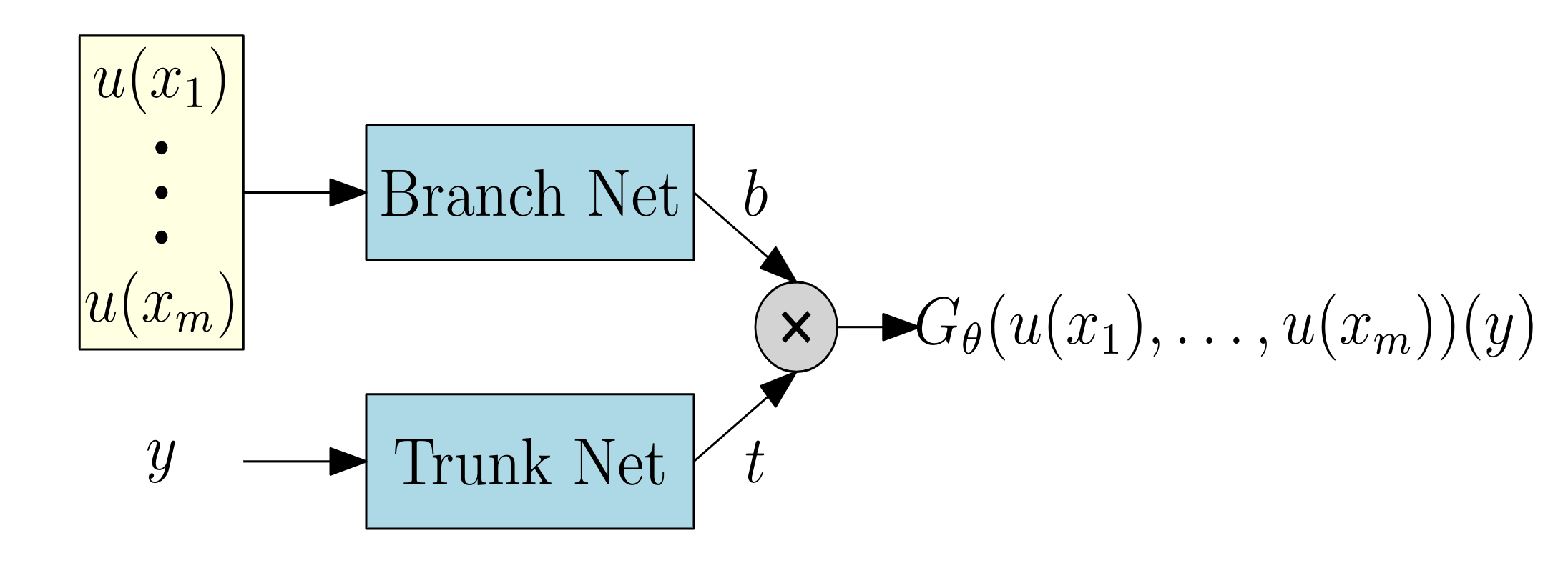
The Branch Net processes the input function information. Let denote points in the domain of (we refer to these points as the sensors), such that is a discrete representation of the input . The Branch Net takes this discretized as the input and outputs a vector of features . On the other hand, the Trunk Net processes points in the domain of the output function. To this end, the Trunk Net takes as the input and outputs a vector of features . Note that since the Trunk Net’s output solely depends on the input coordinates , it is natural to interpret the components of as a collection of basis functions defined on , i.e.,
The output of the DeepONet then combines the output features from the Branch Net and the Trunk Net using an inner product:
| (2) |
From the above, one can interpret the output of the Branch Net as the trainable coefficients for the basis functions produced by the Trunk Net. To simplify our notation, in the rest of this work, we omit writing the DeepONet explicit dependency on the discretized input and use the simplified notation .
Finally, we train the DeepONet to approximate the nonlinear solution operator by minimizing a mean square loss function on the training dataset , i.e.,
| (3) |
In this work, our aim is to desing a Bayesian training framework for DeepONets that enables us to (1) better approximate and (2) estimate the solution/prediction uncertainty. We refer to this framework as the Bayesian DeepONet.
3 The Bayesian DeepONet
To derive the proposed Bayesian DeepONet framework, we consider the scenario when our available operator training targets correspond to scattered noisy measurements of , i.e., . In particular, we assume these measurements are independently Gaussian distributed centered at the latent true operator target value, i.e.,
Here, is an independent Gaussian noise with zero mean and known standard deviation , i.e., . Let denote the noisy dataset of targets; we can then calculate the likelihood as:
| (4) |
To compute the posterior distribution, we use Bayes’ theorem, i.e.,
where “” denotes equality up to a constant. In practice, computing is usually analytically intractable. Hence, to sample from the posterior , we usually use the unnormalized expression .
To predict and estimate the uncertainty of a solution trajectory, denoted as , for a given input and over the mesh of points , we must sample from the posterior and obtain an -ensemble of DeepONet parameters, i.e., . Then, using this ensemble, we can obtain statistics from simulated trajectories . In this work, we compute the mean and standard deviation of . We use the mean to predict the true solution and the standard deviation to quantify the predictive uncertainty.
To sample from the posterior and obtain the -ensemble , in this work, we use replica exchange stochastic Langevin diffusion (re-SGLD) [12], which we review in the next section and detail in Algorithm 1.
3.1 Review of the re-SGLD
To derive re-SGLD (Algorithm 1), we start from the Langevin diffusion, which reads:
| (5) |
where is called the particle and corresponds to the target trainable parameters of the DeepONet, is the Brownian motion in , is the temperature parameter, and is an energy function defined as:
| (6) |
where denotes the prior and the likelihood (4).
To obtain the target parameters, we must solve an optimization problem. More precisely, we must find that minimizes the energy (6). To this end, one can show that, under proper assumptions for the energy function , the sequence of targets converges to the target distribution as [7]. Furthermore, when the temperature parameter is small enough, distributes around the minimizer [18]. Hence, one can obtain the minimizer of the energy (6) by sampling from the target distribution .
In addition, when the temperature is low, the particle tends to reach stationary points with fast local convergence [28], by exploiting the landscape of the energy function . On the other hand, when the temperature is high, the particle tends to traverse globally, exploring the landscape of the energy function . This exploitation-exploration dilemma has led researchers to design algorithms (e.g., re-SGLD) that achieve superior performance by balancing exploration and exploitation.
In this work, we use exploration and exploitation by considering two Langevin equations with separated particles and and different temperatures (low) and (high), i.e.,
| (7a) | |||
| (7b) | |||
Then, by swapping the particles and , with controlled rate , one can help the low-temperature particle to escape the local minima and achieve improved and accelerated convergence.
The theoretical support for the previous claims were established in the convergence result of [5]. That is, the replica exchange Langevin diffusion (re-LD) algorithm, which simulates the dynamics (7) and allows the swapping of particles, i.e., , with rate:
| (8) |
converges to the invariant distribution with density:
| (9) |
3.2 Errors in the energy function
In practice, computing the energy function may fail due to, for example, errors in the dataset or an insufficient number of samples of to represent the likelihood and cover the target output space. Moreover, when the size of the dataset is large, it is expensive to compute . Hence, the authors in [12] proposed to approximate the energy function using a mini-batch of data . In any case, an unbiased estimator of the energy function is then
| (10) |
Moreover, we assume the estimator (10) follows the normal distribution
where is the variance of the estimator. To simulate from the dynamics (5), we discretize them and obtain
| (11a) | |||
| (11b) | |||
where are the positive learning rates and are the energy function estimators of the two particles. However, using the unbiased estimators for the energy, and , in re-LD with discretized dynamics (11) leads to a large bias for the estimator of the swapping rate defined in (8).
To remove the bias from the swaps, we allow the particles swapping with the following unbiased rate estimator [12],
| (12) |
where are two positive constants. The replica exchange algorithm then converges to the target invariant distribution with this new unbiased rate estimator . We refer to this algorithm as the replica exchange stochastic gradient Langevin diffusion (reSGLD) if (see Algorithm 1); otherwise, we refer to the algorithm as the multi-variance replica exchange stochastic gradient Langevin diffusion (m-reSGLD).
4 Accelerated Bayesian training of DeepONets
In this section, we propose exploiting the DeepONet’s architecture to develop an accelerated Bayesian training strategy that (1) reduces the time reSGLD (Algorithm 1) uses to train the DeepONet parameters and (2) achieves a performance comparable to reSGLD. Such training strategy results in a multi-variance replica-exchange SGLD (m-reSGLD) algorithm (Algorithm 2), which we describe next.
Many theoretical results have showed that over-parametrized neural networks, trained with gradient descent-based methods, converge to zero-training loss exponentially fast with the network parameters hardly changing [14, 13]. Motivated by this convergence result, other works have studied whether the same holds for under-parametrized neural networks. Their results [8] show that exponential convergence to zero-training loss can happen, with parameters hardly varying, but depends on an implicit scaling. Motivated by these results, in this work, we propose a more efficient Bayesian framework that trains a less parametrized DeepONet, i.e., a DeepONet that keeps some of its parameters hardly varying during training.
Intuitively, our proposed framework follows from the fact that empirically (see [25]), DeepONets converge exponentially fast to zero-training loss. Hence, we expect that a DeepONet that keeps, during training, some of its parameters hardly varying should also converge to zero-training loss provided an appropriate training regime. In this paper, such a regime corresponds to training the Branch Net or the Trunk Net randomly. We refer to this training regime as the accelerated Bayesian training of DeepONets, which we use to reduce the computational cost of reSGLD.
The reSGLD has demonstrated excellent convergence capabilities when used for training neural networks. However, compared to vanilla SGLD [26], the computational cost of reSGLD doubles. To reduce the computational cost of reSGLD, we adopt the idea proposed in [24] and develop m-reSGLD (Algorithm 2); that is, an algorithm that uses (1) a full training regime for the low temperature particle , which exploits the landscape of the energy function , and (2) a accelerated training regime for the high temperature particle , which explores the landscape of . To this end, we first fully train both particles for a fixed number of burn-in epochs. After burn-in, we let the high temperature particle enter the accelerated training regime. Let us split the high temperature particle into its Branch Net and Trunk Net components, i.e., . Then, to control which sub-network parameters ( or ) are trained more, we define the training control parameter . If , we train more the Branch Net parameters . If, on the other hand, , we train more the Trunk Net paramters .
We select the parameters that we train more based on the DeepONet architecture. As explained in Section 2.1, the DeepONet architecture, depicted in Figure 1 and whose output is given by (2), enables us to interpret the Branch Net output as trainable coefficients for the basis functions produced by the Trunk Net. Hence, DeepONets, as proved in [21], fall within the class of linear approximation methods because they approximate the nonlinear space of the operator via the linear space generated by the Trunk Net, i.e., . Thus, in practice, we choose to train more the Branch Net because its output represents the coefficients of the linear space generated by the Trunk Net.
Let us conclude this section with the following result. If the networks are identical, then the accelerated training regime reduces at most half of the computational cost for . Thus, overall, m-reSGLD reduces at most of the reSGLD computational cost. Finally, one should note that, due to the accelerated regime, the variances of the particles are no longer the same. As result, we use the name multi-variance reSGLD for Algorithm 2.
5 Numerical experiments
In this section, we test the accuracy and efficiency of the proposed Bayesian training framework using four examples: an anti-derivative operator, a gravity pendulum system, a diffusion reaction system, and an advection diffusion system. To train the DeepONets that will approximate the solution operator of each example, we use three frameworks. First, we use the state-of-the-art gradient descent optimization framework Adam (Adam) [20]. We then compare the performance of Adam with the proposed replica exchange stochastic gradient Langevin diffusion (reSGLD) and the accelerated replica exchange framework (m-reSGLD). During training, each framework will be tested systematically using datasets of noisy output targets with different noise values.
Metrics. To test the performance of the frameworks, we compute the and relative errors of a test trajectory. That is, for a given input , we predict using DeepONets the solution of this test trajectory at a collection of selected mesh points . Denote the mean predicted solution of the test trajectory as and the true solution as , then we calculate the relative errors as follows:
| (13) |
In our experiments, we compute mean value of the relative errors for 100 test trajectories selected from outside the training dataset.
We also verify how the three frameworks handle the noisy targets and estimate the predictive uncertainty. To this end, for every test trajectory, we construct a () confidence interval. For reSGLD and m-reSGLD the confidence interval is constructed using the prediction samples obtained, respectively, from Algorithm 1 and Algorithm 2. To enable Adam to estimate uncertainty, we adopt the non-Bayesian framework of dropout [17] and use the strategy described in [27]. To measure how well these confidence intervals quantify uncertainty, we compute the ratio of the true trajectory that is within the confidence interval, i.e.,
| (14) |
5.1 Experiment 1
In this experiment, we use the proposed Bayesian framework to train a DeepONet that approximates the solution operator of the following ordinary differential equation (ode):
| (15) |
with the initial condition is . Note that the solution operator for (15) corresponds to the anti-derivative operator:
Here denotes an external force that drives the response of the ode system (15). We sample this external force from the following mean-zero Gaussian Random Field (GRF):
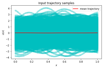
where the covariance kernel is the radial-basis function (RBF) kernel with length-scale parameter . In this experiment, we set the length-scale parameter to . Figure 2 illustrates the distribution of input samples simulated from the GRF and used to train the DeepONets. More specifically, the Branch Net takes the discretized version of these input samples during training. Here, we discretized using sensors.
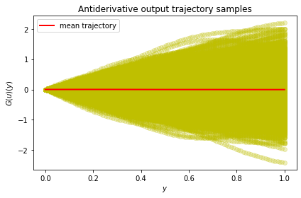
In addition, we present in Figure 3 the distribution of the true operator targets associated with the input samples . We can observe that these targets deviate largely from the mean. Thus, any predictive framework must capture the operator response over the whole output target space. Such a requirement makes this problem very challenging.
5.1.1 Small noise
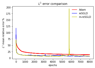
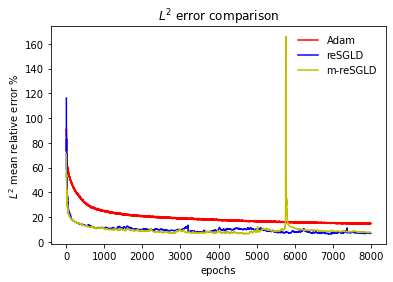
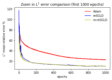
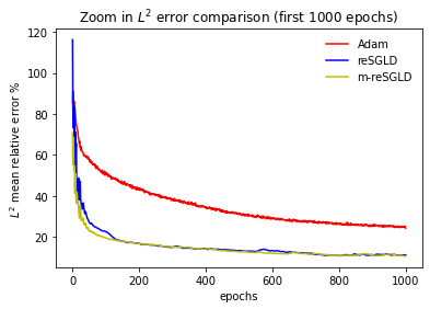
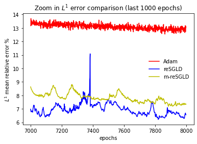
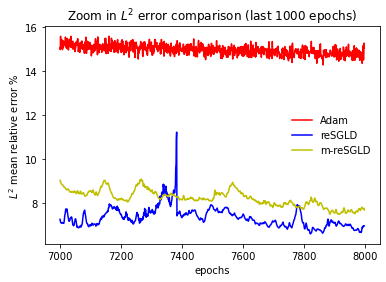
We consider first training the DeepONet using operator targets with small noise. That is, we assume the noise follows the normal distribution . We train the DeepONet for epochs using the three frameworks. And, at each epoch, we compute the mean of the relative errors and of 100 test trajectories. Figure 4 shows how these errors converge during training. Furthermore, Table 1 presents the average mean relative errors the burn-in epochs.
| frameworks | ||
|---|---|---|
| Adam | ||
| reSGLD | ||
| m-reSGLD |
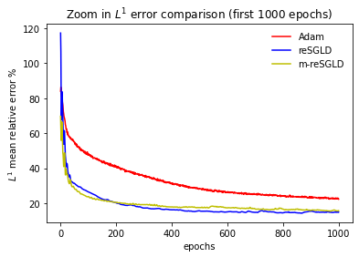
From Figure 4 and Table 1, we can observe that the proposed reSGLD and m-reSGLD converge much faster than Adam. Moreover, the average relative errors after burn-in show that the mean predictive performance of the proposed Bayesian framework outperforms the state-of-the-art Adam. Such improved accuracy illustrates that reSGLD and m-reSGLD handle much better noisy training data.
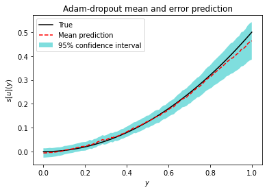
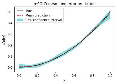
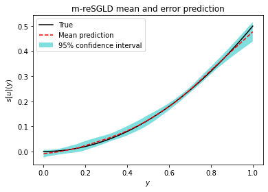
Besides fast training convergence and improved mean predictive performance, we have to check if the proposed frameworks can capture the predictive uncertainty of the problem. To this end, we illustrate in Figure 5, for a randomly selected test trajectory, the confidence interval and the error for Adam with dropout, reSGLD, and m-reSGLD. We observe that the three frameworks capture the true trajectory within their confidence intervals. Adam, however, seems to overestimate its predictive uncertainty, producing a wider confidence band.
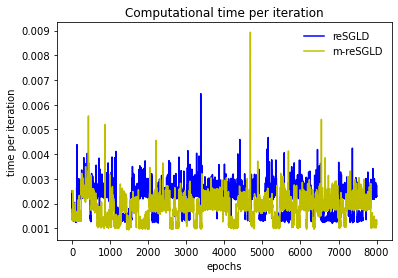
We also verify how much of the computational cost of reSGLD is reduced when using m-reSGLD. To this end, during training, we record the per-iteration computational time for reSGLD and m-reSGLD (see Figure 6). The results show that the computational time for m-reSGLD corresponds to the computational time of reSGLD. This reduction of approximate of the cost of reSGLD is close to the theoretical maximum of . Furthermore, m-reSGLD does not deteriorate the predictive performance of the DeepONet (see Table 1).
5.1.2 Increased noise
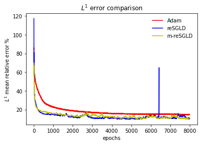
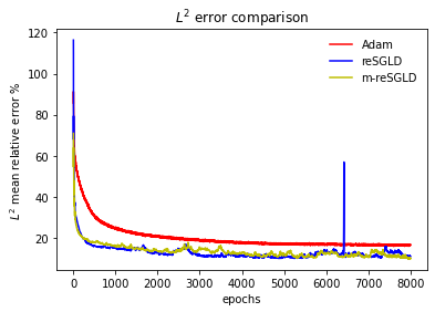
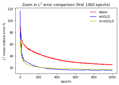
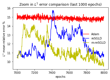
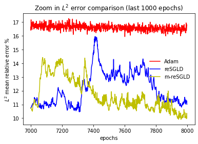
We now verify the performance of the proposed frameworks when the noise associated to the operator output targets increases. In particular, we assume the increased noise follows the normal distribution . Figure 7 depicts the training convergence results for the the relative errors and , and Table 2 presents the average errors.
| frameworks | ||
|---|---|---|
| Adam | ||
| reSGLD | ||
| m-reSGLD |
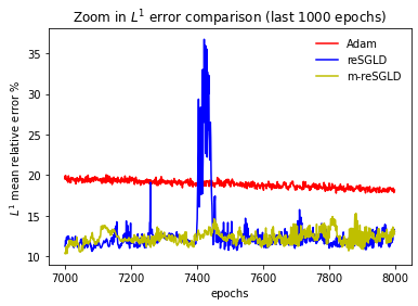
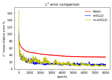
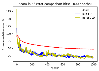
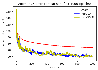
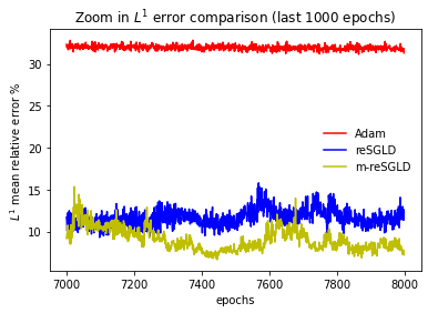
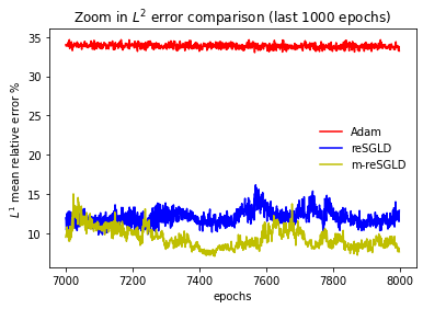
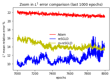
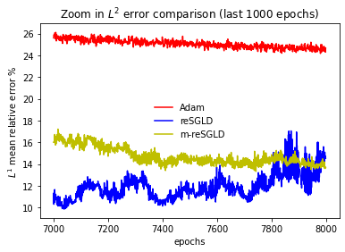
We observe from Figure 7 and Table 2 that the convergence performance of the three frameworks deteriorates in this increased noise scenario. Our proposed frameworks, however, provide a faster training convergence and have much better mean predictive capability than Adam.
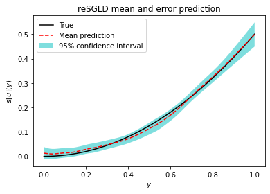
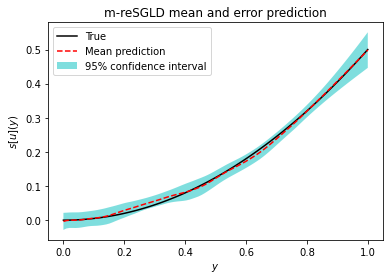
We also construct the confidence intervals for the three frameworks. Figure 8 shows that, as expected, the predictive uncertainty (i.e., the width of the confidence band) estimated by the proposed framework has increased in this scenario. The confidence band for Adam, however, has becomes more noisy and uncertain. Also, we note that the three frameworks capture the true solution trajectory, i.e., they have . Thus, we conclude that the proposed frameworks are more effective in predicting uncertainty in this increased noise scenario.
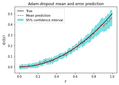
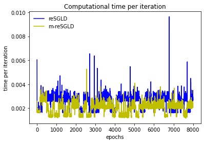
We conclude this experiment by illustrating (see Figure 9) how much computational cost is saved when using m-reSGLD instead of reSGLD. The average per-iteration time (i.e., the computational cost) for m-reSGLD represents of the per-teration time used by reSGLD. Moreover, for this increased noise scenario, m-reSGLD is not only more efficient but also provides a better mean predictive performance (see Table 2).
5.2 Experiment 2
In this experiment, we use the proposed frameworks to train a DeepONet that approximates the solution operator for the following gravity pendulum with external force,
| (16a) | ||||
| (16b) | ||||
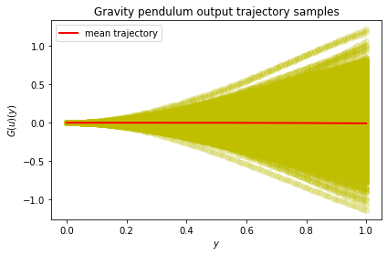
with an initial condition , and . We simulate the discretized external force using a mean-zero GRF with RBF kernel (length-scale parameter ) and sensors. We illustrate in Figure 10 the distribution of the true operator targets associated with the input samples and used to train the gravity pendulum system.
5.2.1 Small noise
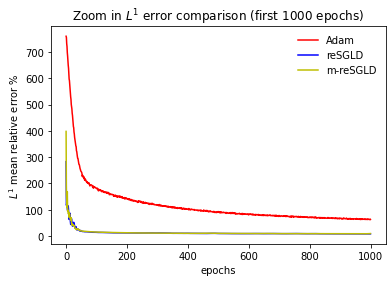
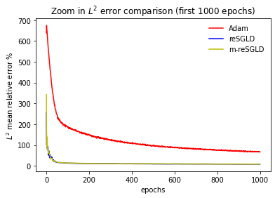
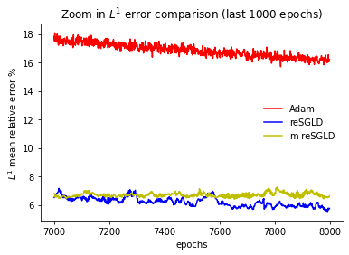
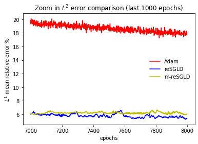
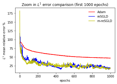
We start by verifying the performance of the proposed frameworks using a small noise scenario. In particular, let us assume the noise for the target outputs follows the normal distribution . We train the DeepONet for epochs using the three frameworks. Figure 11 shows the convergence results for the errors and during training. And Table 3 presents the average of these errors after the burn-in epochs. The results show that the proposed frameworks converge much faster during training and provide better mean prediction performance than the state-of-the-art optimization algorithm Adam.


| frameworks | ||
|---|---|---|
| Adam | ||
| reSGLD | ||
| m-reSGLD |
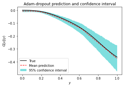
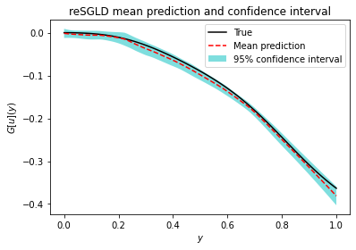
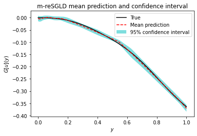
To test how well the proposed frameworks estimate the uncertainty, we select at random one test trajectory and plot, in Figure 12, the estimated confidence intervals. Figure 12 shows that the proposed frameworks capture the true test trajectory within their confidence interval, i.e., . Adam, on the other hand, not only fails to capture the whole true trajectory (), but also overestimates the predictive uncertainty by producing a wider confidence band in some regions.
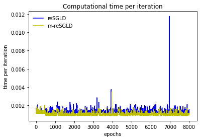
To this end, we compare the computational cost of reSGLD and m-reSGLD, we plot in Figure 13 the per-iteration running time for both frameworks. We observe that the per-iteration time for m-reSGLD is smaller than that for reSGLD. Thus, the computational cost for m-reSGLD represents of the computational cost for reSGLD. Such a reduction is achieved by m-reSGLD without compromising mean predictive accuracy (see Table 3).
5.2.2 Increased noise
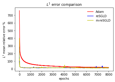
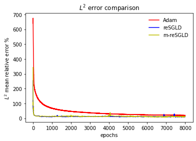
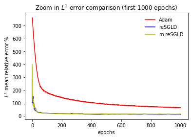
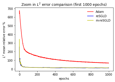
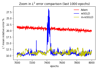
In this section, we verify the performance of the DeepONets when the variance of noise for the operator targets increases. In particular, we assume the noise follows the normal distribution . Figure 14 and Table 4 detail the convergence errors for this increased noise scenario. Similar to the anti-derivative example, the convergence results deteriorate when the noise increases. However, compared with Adam, the proposed frameworks still provide improved training convergence and mean prediction performance.
| frameworks | ||
|---|---|---|
| Adam | ||
| reSGLD | ||
| m-reSGLD |
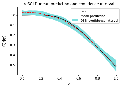
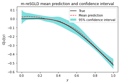
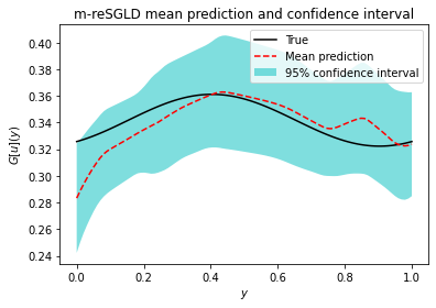
The constructed confidence intervals for the three frameworks in this increased noise scenario are depicted in Figure 15. We observe that the proposed frameworks have a wider confidence band. This is expected since the increase in noise variance leads to larger uncertainty. Adam, however, seems to not change its estimate for this increased noise scenario. Furthermore, compared to Adam , we note that the proposed frameworks capture fairly well the true trajectory with their estimated confidence intervals (reSGLD: and m-reSGLD: ).

We conclude this gravity pendulum example by illustrating in Figure 16 the per-iteration time used by reSGLD and m-reSGLD. The results show that the computational cost of m-reSGLD corresponds to of the computational cost of reSGLD. As before, m-reSGLD achieves such a reduction without compromising the mean prediction performance.
5.3 Experiment 3
In our third experiment, we test the performance of the proposed Bayesian DeepONet with the following diffusion reaction equation,
| (17a) | |||
| (17b) | |||
| (17c) | |||
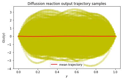
where and . Similar to the previous examples, the input samples are simulated using the GRF (see Figure 2) and discretized using sensors. Figure 17 shows the distribution of the true operator targets associated to the input samples for the diffusion reaction system.
5.3.1 Small noise
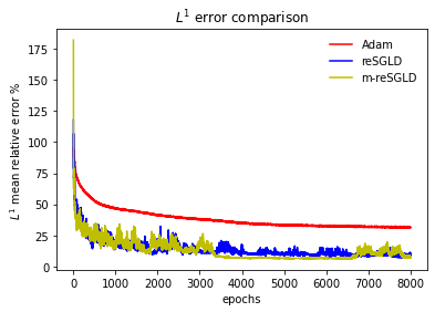
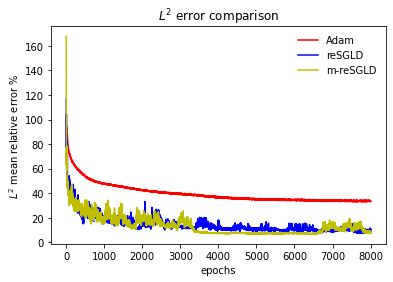
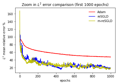
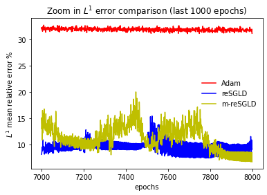
In this small noise scenario, the noise added to the operator targets follows the normal distribution . We train the DeepONet for epochs. Figure 18 shows the convergence results of the relative errors and during training. Also, Table 5 presents the average of these relative errors after the burn-in epochs. Compared to the state-of-the-art Adam optimizer, the results show that the proposed frameworks (reSGLD and m-reSGLD) present improved training convergence and mean prediction performance.

| frameworks | ||
|---|---|---|
| Adam | ||
| reSGLD | ||
| m-reSGLD |
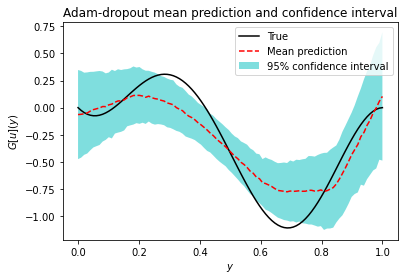
We also show in Figure 19 the estimated confidence intervals for the three frameworks. The results show that Adam with dropout over-estimates the uncertainty (wider confidence band in some regions), but fails to capture the whole true test trajectory () within the confidence interval. On the other hand, the proposed frameworks, reSGLD and m-reSGLD, provide a more balanced confidence intervals that can capture the whole true trajectory ().
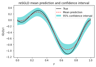
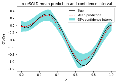
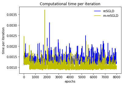
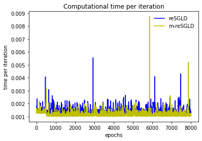
For this small noise scenario, we plot in Figure 20 the per-iteration time consumed by the proposed frameworks reSGLD and m-reSGLD. Note that by using m-reSGLD we can save of the computational cost of re-SGLD. Furthermore, m-reSGLD achieves such a reduction without sacrificing the mean predictive performance (see Table 5).
5.3.2 Increased noise
In this section, we increase the noise variance so that the noise follows the normal distribution . Figure 21 shows the convergence results of and relative errors during training. Moreover, Table 6 presents the average of these errors after the burn-in. Compared to Adam, we observe that the proposed frameworks present improved mean prediction performance and training convergence.
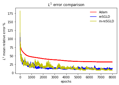
| frameworks | ||
|---|---|---|
| Adam | ||
| reSGLD | ||
| m-reSGLD |
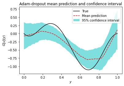
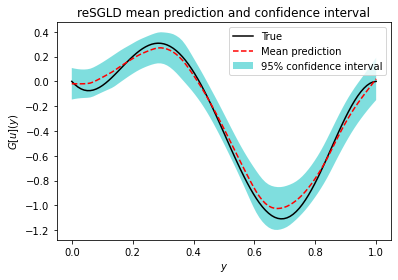
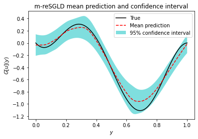
The estimated confidence intervals are depicted in Figure 22. Clearly, the proposed frameworks capture much better the true trajectory in their confidence intervals . Adam, on the other hand, seems affected by the noise and fails to capture the whole trajectory .
We conclude this example by plotting the per-iteration time for reSGLD and m-reSGLD (Figure 23). We conclude that m-reSGLD uses only of the computational resources used by reSGLD. Such a reduction is achieved by the proposed m-reSGLD with (remarkably) improved prediction performance (see Table 6).
5.4 Experiment 4
In our final experiment, we verify the effectiveness of the proposed Bayesian DeepONet using the following advection-diffusion system with periodic boundary conditions,
| (18) | ||||
| (19) |
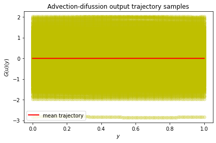
where , , . Here is an initial condition sampled from a GRF with an RBF kernel of length scale and discretized using sensors. We show in Figure 24 the distribution of the true operator targets associated with the input samples .
5.4.1 Small noise
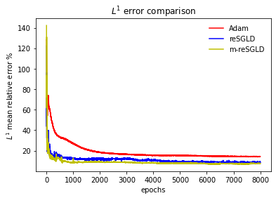
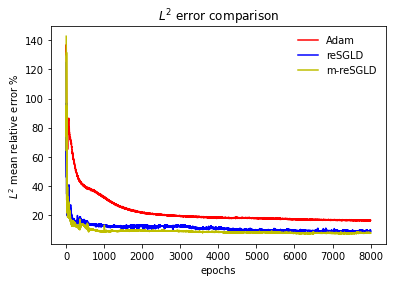
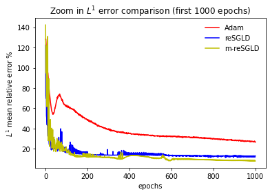
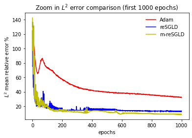
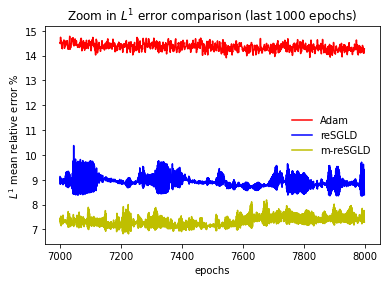
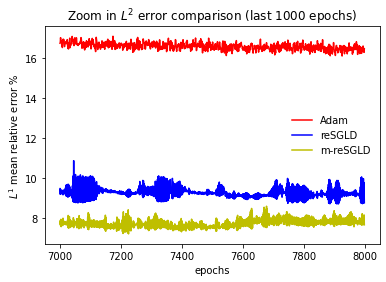
In the small noise scenario, we assume the training operator targets are corrupted by noise that follows the normal distribution . We train the DeepONets for epochs. Figure 25 shows the convergence errors and and Table 7 presents the average of these errors after the burn-in epochs. From Figure 25 and Table 7, we conclude that reSGLD and m-reSGLD have faster training converge and better mean prediction performance than Adam.
| frameworks | ||
|---|---|---|
| Adam | ||
| reSGLD | ||
| m-reSGLD |
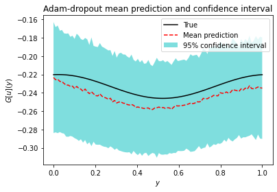
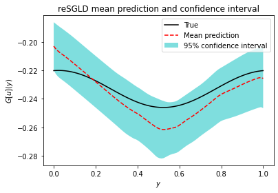
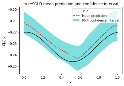
To illustrate how well our Bayesian DeepONet estimates the uncertainty, we select one test trajectory and plot, in Figure 26, the estimated confidence interval by the three frameworks. We observe that the three methods capture the true trajectory . Adam, however, seems to over-estimate the uncertainty, yielding a wider confidence band.
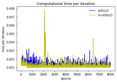
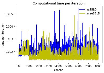
We conclude this section by plotting (Figure 27) the per-iteration time consumed by the proposed frameworks reSGLD and m-reSGLD. We observe that The average computation time of m-reSGLD is around of reSGLD framework. The proposed accelerated training regime m-reSGLD achieves such a reduction even with improved mean prediction performance (see Table 7).
5.4.2 Increased noise
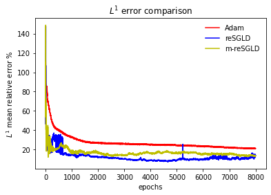
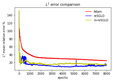
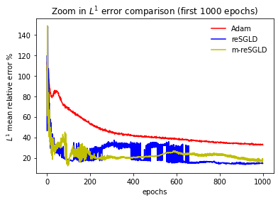
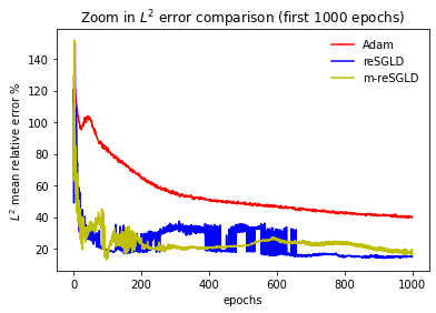
Finally, we verify the performance of the proposed Bayesian DeepONet when the variance of the noise for the operator targets increases. In particular, for the advection-diffusion example, we assume the increased noise follows the normal distribution . Figure 28 and Table 8 detail the convergence errors for this increased noise scenario. Similar to our previous experiments, the proposed frameworks present improved training convergence and better mean prediction performance than Adam. This shows that the proposed frameworks handle noise more effectively.
| frameworks | ||
|---|---|---|
| Adam | ||
| reSGLD | ||
| m-reSGLD |
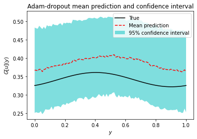
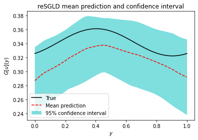
We verify next how well the DeepONets capture uncertainty in this increased noise scenario. To this end, we select at random a test trajectory and plot the estimated confidence intervals in Figure 29. The results show that, as expected, the proposed frameworks are more uncertain in this increased noise scenario, capturing the whole true test trajectory (). Adam, on the other hand, seems to provide the same estimate of uncertainty as for the small noise scenario.
We also plot the per-iteration time used by re-SGLD and m-reSGLD in Figure LABEL:advd_v90_time. We observe that m-reSGLD is more efficient; it consumes only of the computational cost of re-SGLD.
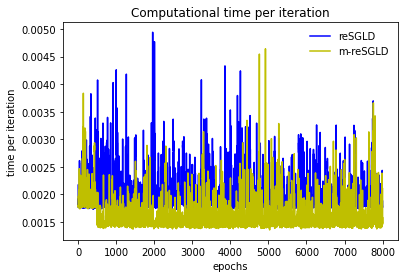
To conclude this section, we would like to remark that for all the examples above, we can conclude that reSGLD and m-reSGLD converge much faster than Adam during training, with improved prediction accuracy. The proposed frameworks, reSGLD and m-reSGLD, are able to handle the noise in the training data and capture the true solutions within the estimated confidence intervals. The performance of Adam, on the other hand, deteriorates for the increased noise scenario. The benefit of the accelerated training regime of m-reSGLD is that it saves up to 25% of the computational cost of reSGLD. Such savings are achieved without deteriorating predictive performance. In fact, in some of the examples, m-reSGLD (remarkably) has even better prediction accuracy than reSGLD.
6 Conclusion
In this work, we study the problem of approximating the solution operator of parametric PDEs using the Deep Operator Network (DeepONet) framework and noisy data. To this end, we propose using the Bayesian framework of replica-exchange Langevin diffusion. The replica-exchange ability to escape local minima (using one particle to explore and another to exploit the loss function landscape of DeepONets) enables the proposed framework to provide (1) improved training convergence in noisy scenarios, and (2) (remarkably) enhanced predictive capability compared to vanilla DeepONets trained using state-of-the-art gradient-based optimization (e.g., Adam). We also demonstrate that the proposed framework effectively estimates the uncertainty of approximating solution trajectories of parametric PDEs. To reduce the computational cost of replica, due to the doubled computational cost of using two particles, we propose an accelerated replica-exchange algorithm that randomly chooses to train one of the DeepONet sub-networks while keeping the other fixed. Using a series of systematically designed experiments, we demonstrate that this accelerated replica-exchange algorithm can save up to 25% of the original replica-exchange algorithm’s original cost without compromising the DeepONet’s performance. In our future work, we will study the theoretical aspect of this accelerated replica-exchange framework.
References
- [1] K. Bhattacharya, B. Hosseini, N. B. Kovachki, and A. M. Stuart. Model reduction and neural networks for parametric pdes. arXiv preprint arXiv:2005.03180, 2020.
- [2] S. Cai, Z. Wang, L. Lu, T. A. Zaki, and G. E. Karniadakis. Deepm&mnet: Inferring the electroconvection multiphysics fields based on operator approximation by neural networks. Journal of Computational Physics, 436:110296, 2021.
- [3] T. Chen and H. Chen. Universal approximation to nonlinear operators by neural networks with arbitrary activation functions and its application to dynamical systems. IEEE Transactions on Neural Networks, 6(4):911–917, 1995.
- [4] T. Chen, E. Fox, and C. Guestrin. Stochastic gradient hamiltonian monte carlo. In International conference on machine learning, pages 1683–1691. PMLR, 2014.
- [5] Y. Chen, J. Chen, J. Dong, J. Peng, and Z. Wang. Accelerating nonconvex learning via replica exchange langevin diffusion. arXiv preprint arXiv:2007.01990, 2020.
- [6] B. Chetverushkin, E. Chung, Y. Efendiev, S.-M. Pun, and Z. Zhang. Computational multiscale methods for quasi-gas dynamic equations. Journal of Computational Physics, 440:110352, 2021.
- [7] T.-S. Chiang, C.-R. Hwang, and S. J. Sheu. Diffusion for global optimization in r^n. SIAM Journal on Control and Optimization, 25(3):737–753, 1987.
- [8] L. Chizat, E. Oyallon, and F. Bach. On lazy training in differentiable programming. arXiv preprint arXiv:1812.07956, 2018.
- [9] E. Chung, Y. Efendiev, W. T. Leung, S.-M. Pun, and Z. Zhang. Multi-agent reinforcement learning accelerated mcmc on multiscale inversion problem. arXiv preprint arXiv:2011.08954, 2020.
- [10] E. Chung, Y. Efendiev, S.-M. Pun, and Z. Zhang. Computational multiscale methods for parabolic wave approximations in heterogeneous media. arXiv preprint arXiv:2104.02283, 2021.
- [11] E. Chung, W. T. Leung, S.-M. Pun, and Z. Zhang. A multi-stage deep learning based algorithm for multiscale model reduction. Journal of Computational and Applied Mathematics, 394:113506, 2021.
- [12] W. Deng, Q. Feng, L. Gao, F. Liang, and G. Lin. Non-convex learning via replica exchange stochastic gradient mcmc. In International Conference on Machine Learning, pages 2474–2483. PMLR, 2020.
- [13] S. Du, J. Lee, H. Li, L. Wang, and X. Zhai. Gradient descent finds global minima of deep neural networks. In International Conference on Machine Learning, pages 1675–1685. PMLR, 2019.
- [14] S. S. Du, X. Zhai, B. Poczos, and A. Singh. Gradient descent provably optimizes over-parameterized neural networks. arXiv preprint arXiv:1810.02054, 2018.
- [15] Y. Efendiev, W. T. Leung, G. Lin, and Z. Zhang. Hei: hybrid explicit-implicit learning for multiscale problems. arXiv preprint arXiv:2109.02147, 2021.
- [16] S. Fresca, L. Dede, and A. Manzoni. A comprehensive deep learning-based approach to reduced order modeling of nonlinear time-dependent parametrized pdes. Journal of Scientific Computing, 87(2):1–36, 2021.
- [17] Y. Gal and Z. Ghahramani. Dropout as a bayesian approximation: Representing model uncertainty in deep learning. In international conference on machine learning, pages 1050–1059. PMLR, 2016.
- [18] C.-R. Hwang. Laplace’s method revisited: weak convergence of probability measures. The Annals of Probability, pages 1177–1182, 1980.
- [19] Y. Khoo, J. Lu, and L. Ying. Solving parametric pde problems with artificial neural networks. European Journal of Applied Mathematics, 32(3):421–435, 2021.
- [20] D. P. Kingma and J. Ba. Adam: A method for stochastic optimization. arXiv preprint arXiv:1412.6980, 2014.
- [21] N. Kovachki, Z. Li, B. Liu, K. Azizzadenesheli, K. Bhattacharya, A. Stuart, and A. Anandkumar. Neural operator: Learning maps between function spaces. arXiv preprint arXiv:2108.08481, 2021.
- [22] I. M. S. Leite, J. D. M. Yamim, and L. G. d. Fonseca. The deeponets for finance: An approach to calibrate the heston model. In EPIA Conference on Artificial Intelligence, pages 351–362. Springer, 2021.
- [23] C. Lin, Z. Li, L. Lu, S. Cai, M. Maxey, and G. E. Karniadakis. Operator learning for predicting multiscale bubble growth dynamics. The Journal of Chemical Physics, 154(10):104118, 2021.
- [24] G. Lin, Y. Wang, and Z. Zhang. Multi-variance replica exchange stochastic gradient mcmc for inverse and forward bayesian physics-informed neural network. arXiv preprint arXiv:2107.06330, 2021.
- [25] L. Lu, P. Jin, G. Pang, Z. Zhang, and G. E. Karniadakis. Learning nonlinear operators via deeponet based on the universal approximation theorem of operators. Nature Machine Intelligence, 3(3):218–229, 2021.
- [26] M. Welling and Y. W. Teh. Bayesian learning via stochastic gradient langevin dynamics. In Proceedings of the 28th international conference on machine learning (ICML-11), pages 681–688. Citeseer, 2011.
- [27] D. Zhang, L. Lu, L. Guo, and G. E. Karniadakis. Quantifying total uncertainty in physics-informed neural networks for solving forward and inverse stochastic problems. Journal of Computational Physics, 397:108850, 2019.
- [28] Y. Zhang, P. Liang, and M. Charikar. A hitting time analysis of stochastic gradient langevin dynamics. In Conference on Learning Theory, pages 1980–2022. PMLR, 2017.
- [29] Z. Zhang, E. T. Chung, Y. Efendiev, and W. T. Leung. Learning algorithms for coarsening uncertainty space and applications to multiscale simulations. Mathematics, 8(5):720, 2020.