Low-Rank+Sparse Tensor Compression for Neural Networks

Abstract

Low-rank tensor compression has been proposed as a promising approach to reduce the memory and compute requirements of neural networks for their deployment on edge devices. Tensor compression reduces the number of parameters required to represent a neural network weight by assuming network weights possess a coarse higher-order structure. This coarse structure assumption has been applied to compress large neural networks such as VGG and ResNet. However modern state-of-the-art neural networks for computer vision tasks (i.e. MobileNet, EfficientNet) already assume a coarse factorized structure through depthwise separable convolutions, making pure tensor decomposition a less attractive approach. We propose to combine low-rank tensor decomposition with sparse pruning in order to take advantage of both coarse and fine structure for compression. We compress weights in SOTA architectures (MobileNetv3, EfficientNet, Vision Transformer) and compare this approach to sparse pruning and tensor decomposition alone.

1 Introduction

Using machine learning to enable multiple applications on edge devices requires multiple task-specific persistent models (Yang et al., 2020). These models are used for tasks ranging from computer vision (Howard et al., 2019) to automatic speech recognition (Wang et al., 2021). The trend towards multiple applications and multiple models is constrained by the fact that off-chip memory reads incur high latency and power costs (Sze et al., 2017). Therefore, in this paper we target memory cost reduction. In this area low-rank tensor compression is a popular approach (Garipov et al., 2016; Novikov et al., 2015; Lebedev et al., 2014) that can achieve orders of magnitude compression, but can lead to significant accuracy loss.

Low-rank tensor compression has achieved impressive headline compression numbers (Garipov et al., 2016) and is suitable for on-device acceleration (Zhang et al., May 2021; Deng et al., 2019) due to its reliance on standard dense linear algebra operations. However it is often applied to massively overparameterized architectures such as VGG or ResNet (Novikov et al., 2015; Hawkins & Zhang, 2019). Recent work benchmarking sparse pruning (Blalock et al., 2020) raises the issue that compression techniques applied to overparameterized architectures may not reach the compression/accuracy Pareto frontier of SOTA compressed networks such as EfficientNet. Further, tensor compression enforces low-rank factorized structure on neural network weights. This factorized structure is already exploited by SOTA computer vision backbones via depth-wise separable convolutions. This motivates us to consider the following question: how can low-rank tensor compression contribute to SOTA computer vision architectures? In this paper we investigate whether low-rank tensor compression can be combined with sparse pruning to capture complementary coarse and fine structures respectively and outperform either sparse pruning or low-rank tensor factorization alone.

Specifically, we investigate two forms of low-rank plus sparse decomposition of neural network weights. First we consider additive structure in which the neural network weights can be decomposed as the sum of a low-rank component and a sparse component. Second we consider a low-rank or sparse structure in which the entries of neural network weights are taken from either a sparse pruned weight or a low-rank weight.

1.1 Related Work

Existing work has studied the combination of low-rank matrices and sparse representations to compress VGG-style models (Yu et al., 2017) and ResNets (Gui et al., 2019). These methods apply additive low-rank plus sparse compression to the weights of neural networks and can achieve compression results that outperform sparse compression or low-rank compression alone. More recent work suggests that low-rank structure is a viable compression method for the EfficientNet model class (Gu et al., 2021) on CIFAR-10/100 computer vision tasks. An open question is whether low-rank matrix or tensor structure remains for efficient modern networks trained on ImageNet.

1.2 Contributions

Our main contribution is our study of low-rank structure remaining in recent SOTA efficient neural networks for computer vision tasks. We observe that trends in architecture design (Howard et al., 2017; Sandler et al., 2018; Howard et al., 2019) have removed low-rank structure from such networks by building in factorized weights. Therefore the direct application of low-rank matrix and tensor methods is challenging. To the best of our knowledge, our work is the first to consider the combination of low-rank tensor compression with sparse pruning. Further, our work is the first to study low-rank+sparse compression of weights for SOTA architectures that rely on efficient depthwise separable convolutions.

Figure 1: High-level proposed algorithm flow.

2 Background

2.1 Tensor Formats

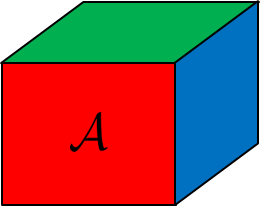
We follow the notation and exposition of (Hawkins et al., 2020) to describe the low-rank tensor formats that we employ. This paper uses lower-case letters (e.g., $a$) to denote scalars, bold lowercase letters (e.g., $\mathbf{a}$) to represent vectors, bold uppercase letters (e.g., $\mathbf{A}$) to represent matrices, and bold calligraphic letters (e.g., $\mathbfcal{A}$) to denote tensors. A tensor is a generalization of a matrix, or a multi-way data array. An order-$d$ tensor is a $d$-way data array $\mathbfcal{A}\in\mathbb{R}^{I_{1}\times I_{2}\times\dots\times I_{d}}$, where $I_{n}$ is the size of mode $n$. The $(i_{1},i_{2},\cdots,i_{d})$-th element of $\mathbfcal{A}$ is denoted as $a_{i_{1}i_{2}\cdots i_{d}}$. An order-$3$ tensor is shown in Fig. 2 (a).

The number of entries in a tensor with mode size $n$ and $d$ modes is $n^{d}$. This exponential dependence on the tensor order is often referred to as the “curse of dimensionality" and can lead to high costs in both computing and storage. Fortunately, many practical tensors have a low-rank structure, and this property can be exploited to reduce such costs. We will use four tensor decomposition formats (CP, Tucker, and TT/TTM) to reduce the parameters of neural networks.

First, we introduce a necessary decomposition to describe the CP format.

Definition 1

A $d$-way tensor $\mathbfcal{A}\in\mathbb{R}^{I_{1}\times\cdots\times I_{d}}$ is rank-1 if it can be written as a single outer product of $d$ vectors

$$\mathbfcal{A}=\mathbf{u}^{(1)}\circ\dots\circ\mathbf{u}^{(d)},\;{\text{with}}\;\mathbf{u}^{(n)}\in\mathbb{R}^{I_{n}}\;\text{for}\;n=1,\cdots,d.$$

Each element of $\mathbfcal{A}$ is $a_{i_{1}i_{2}\cdots i_{d}}=\prod\limits_{n=1}^{d}u_{i_{n}}^{(n)}$, where $u_{i_{n}}^{(n)}$ is the $i_{n}$-th element of the vector $\mathbf{u}^{(n)}$.

Definition 2

The CP factorization (Carroll & Chang, 1970; Harshman et al., 1994) expresses tensor $\mathbfcal{A}$ as the sum of multiple rank-1 tensors:

$$\mathbfcal{A}=\sum_{j=1}^{R}\mathbf{u}_{j}^{(1)}\circ\mathbf{u}_{j}^{(2)}\dots\circ\mathbf{u}_{j}^{(d)}.$$ (1)

Here $\circ$ denotes an outer product operator. The minimal integer $R$ that ensures the equality is called the CP rank of $\mathbfcal{A}$. To simplify notation we collect the rank-1 terms of the $n$-th mode into a factor matrix $\mathbf{U}^{(n)}\in\mathbb{R}^{I_{n}\times R}$ with $\mathbf{U}^{(n)}(:,j)=\mathbf{u}_{j}^{(n)}$. A rank-$R$ CP factorization can be described with $d$ factor matrices $\{\mathbf{U}^{(n)}\}_{n=1}^{d}$ using $R\sum_{n}I_{n}$ parameters.

(a)

(b)

(c)

(d)

Figure 2: Taken from Hawkins et al. (2020). (a): An order-3 tensor, (b) and (c): representations in CP and Tucker formats respectively, where low-rank factors are color-coded to indicate the corresponding modes. (d): TT representation of an order-$d$ tensor, where the purple lines and squares indicate $\mathbfcal{G}^{(n)}(:,i_{n},:)$, which is the $i_{n}$-th slice of the TT core $\mathbfcal{G}^{(n)}$ obtained by fixing its second index.

Next we introduce a prerequisite definition for the low-rank Tucker format.

Definition 3

The mode-$n$ product of a tensor $\mathbfcal{A}\in\mathbb{R}^{I_{1}\times\dots\times I_{n}\times\dots\times I_{d}}$ with a matrix $\mathbf{U}\in\mathbb{R}^{J\times I_{n}}$ is

$$\begin{split}\mathbfcal{B}&=\mathbfcal{A}\times_{n}\mathbf{U}\Longleftrightarrow b_{i_{1}\dots i_{n-1}ji_{n+1}\dots i_{d}}=\sum_{i_{n}=1}^{I_{n}}a_{i_{1}\dots i_{d}}u_{ji_{n}}.\end{split}$$ (2)

The result is still a $d$-dimensional tensor $\mathbfcal{B}$, but the mode-$n$ size becomes $J$. In the special case $J=1$, the $n$-th mode diminishes and $\mathbfcal{B}$ becomes an order-$d-1$ tensor. The Tucker format is defined by a series of mode$-n$ products between a small core tensor and several factor matrices.

Definition 4

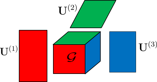
The Tucker factorization (Tucker, 1966) expresses a $d$-way tensor $\mathbfcal{A}$ as a series of mode-$n$ products:

$$\mathbfcal{A}=\mathbfcal{G}\times_{1}\mathbf{U}^{(1)}\times_{2}\dots\times_{d}\mathbf{U}^{(d)}.$$ (3)

Here $\mathbfcal{G}\in\mathbb{R}^{R_{1}\times\dots\times R_{d}}$ is a small core tensor, and $\mathbf{U}^{(n)}\in\mathbb{R}^{I_{n}\times{R}_{n}}$ is a factor matrix for the $n$-th mode. The Tucker rank is the tuple $(R_{1},\dots,R_{d})$. A Tucker factorization with ranks $R_{n}=R$ requires $R^{d}+R\sum_{n}I_{n}$ parameters.

The product structure permits more expressive cross-dimension interactions than the CP model but may not result in large parameter reductions due to the exponential dependence on the tensor order $d$.

Finally we introduce two formats, Tensor-Train and Tensor-Train Matrix. Like the Tucker format, these formats permit more expressive interactions across dimensions. Unlike the Tucker format these formats remove the exponential dependence on the tensor order $d$.

Definition 5

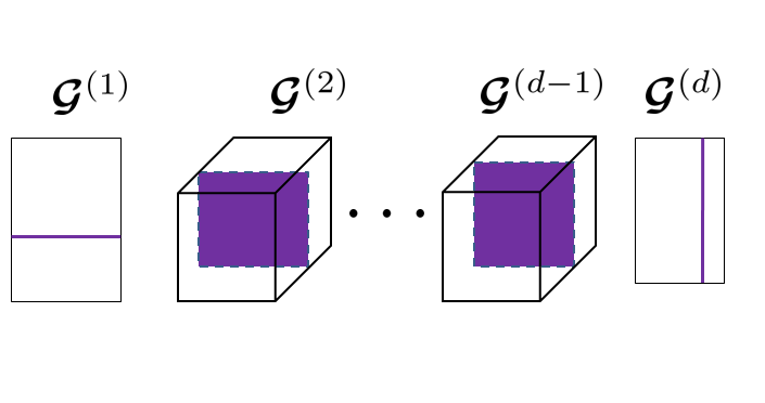
The tensor-train (TT) factorization (Oseledets, 2011) expresses a $d$-way tensor $\mathbfcal{A}$ as a collection of matrix products:

$$a_{i_{1}i_{2}\dots i_{d}}=\mathbfcal{G}^{(1)}(:,i_{1},:)\mathbfcal{G}^{(2)}(:,i_{2},:)\dots\mathbfcal{G}^{(d)}(:,i_{d},:).$$ (4)

Each TT-core $\mathbfcal{G}^{(n)}\in\mathbb{R}^{R_{n-1}\times I_{n}\times R_{n}}$ is an order-$3$ tensor. The tuple $(R_{0},R_{1},\dots,R_{d})$ is the TT-rank and $R_{0}=R_{d}=1$.

The TT format uses $\sum_{n}R_{n-1}I_{n}R_{n}$ parameters in total and leads to more expressive interactions than the CP format.

The TT-format is well-suited to tensors, but is equivalent to low-rank matrix format when the order is $d=2$. We can extend the TT-format to matrices by reshaping along each mode. Let $\mathbf{A}\in\mathbb{R}^{I\times J}$ be a matrix. We assume that $I$ and $J$ can be factored as follows:

$$I=\prod_{n=1}^{d}I_{n},J=\prod_{n=1}^{d}J_{n}.$$ (5)

We can reshape $\mathbf{A}$ into a tensor $\mathbfcal{A}$ with dimensions $I_{1}\times\dots\times I_{d}\times J_{1}\times\dots\times J_{d}$, such that the $(i,j)$-th element of $\mathbf{A}$ uniquely corresonds to the $(i_{1},i_{2},\cdots,i_{d},j_{1},j_{2},\cdots,j_{d})$-th element of $\mathbfcal{A}$. The TT decomposition can extended to compress the resulting order-$2d$ tensor as follows.

Definition 6

The tensor-train matrix (TTM) factorization expresses an order-$2d$ tensor $\mathbfcal{A}$ as $d$ matrix products:

$$a_{i_{1}\dots i_{d}j_{1}\dots j_{d}}=\mathbfcal{G}^{(1)}(:,i_{1},j_{1},:)\mathbfcal{G}^{(2)}(:,i_{2},j_{2},:)\dots\mathbfcal{G}^{(d)}(:,i_{d},j_{d},:).$$ (6)

Each TT-core $\mathbfcal{G}^{(n)}\in\mathbb{R}^{R_{n-1}\times I_{n}\times J_{n}\times R_{n}}$ is an order $4$ tensor. The tuple $(R_{0},R_{1},R_{2},\dots,R_{d})$ is the TT-rank and as before $R_{0}=R_{d}=1$. This TTM factorization requires $\sum_{n}R_{n-1}I_{n}J_{n}R_{n}$ parameters to represent $\mathbfcal{A}$.

We provide a visual representation of the CP, Tucker, and TT formats in Fig. 2 (b) – (d).

2.2 Folding to high-order tensors.

In the previous section we described how to adapt the TT format to the matrix case by factorizing the dimensions of a matrix and viewing the matrix as a tensor. Our goal is to apply tensor decompositions to the weights of many architectures that include $1\times 1$ convolutions (MobileNet, EfficientNet) or fully-connected layers (Vision Transformer). These matrix-format weights are well-suited to the TTM decomposition, but not the CP and Tucker formats which collapse to low-rank matrix format. To apply the CP and Tucker decompositions to these matrix weights we can perform a reshape operation. A weight matrix $\mathbf{W}\in\mathbb{R}^{I\times J}$ can be folded into an order-$d$ tensor $\mathbfcal{A}\in\mathbb{R}^{I_{1}\times\dots\times I_{d}}$ where $IJ=\prod_{n}I_{n}$. We can also fold $\mathbf{W}$ to an order-$2d$ tensor $\mathbfcal{A}\in\mathbb{R}^{I_{1}\times\cdots\times I_{d}\times J_{1}\times\cdots\times J_{d}}$ such that $w_{ij}=a_{i_{1}\cdots i_{d}j_{1}\cdots j_{d}}$. While a convolution filter is already a tensor, we can reshape it to a higher-order tensor with reduced mode sizes. Reshaping imposes additional higher-order and hierarchical tensor structure.

2.3 Sparse Pruning

We prune a tensor weight $\mathbfcal{S}$ by applying a binary tensor mask $\mathbfcal{M}$ to $\mathbfcal{S}$ using the entry-wise product

$$(\mathbfcal{M}\odot\mathbfcal{S})_{i_{1}\dots i_{d}}=m_{i_{1}\dots i_{d}}\times s_{i_{1}\dots i_{d}}.$$

We focus on global magnitude pruning LeCun et al. (1990) throughout this work and use a cubic pruning schedule taken from Zhu & Gupta (2017). At each step we mask the bottom $100\times(s_{t}-s_{t-1})$ percent of the non-masked weights in $\mathbfcal{S}$ by setting their corresponding entries in $\mathbfcal{M}$ to zero where

$$s_{t}=s_{f}\left(\frac{t}{n}\right)^{3}$$ (7)

and $s_{f}$ is the desired final sparsity ratio, $t$ is the current step, and $n$ is the total number of steps. This process gradually increases the sparsity in $\mathbfcal{M}$ until the target sparsity $s_{f}$ is reached.

2.4 Distillation

The goal of knowledge distillation is to transfer the knowledge of an expensive teacher model to a cheaper student model (Hinton et al., 2015). In this setting “expensive" refers to the memory cost of storing the neural network weights. The expensive teacher model $f_{t}$ is a neural network pretrained on ImageNet. The student model $f_{s}$ is the compressed teacher model obtained through sparse pruning and/or tensor compression. Given a training example with input $\mathbf{x}$ and label $\mathbf{y}$ the knowledge distillation loss is

$$\mathcal{L}\left(\mathbf{x},\mathbf{y}\right)=\alpha l(\mathbf{x},\mathbf{y})+(1-\alpha)T^{2}KL\left(f_{s}(\mathbf{x})/T||f_{t}(\mathbf{x})/T\right)$$ (8)

where $l$ is any standard loss function and $KL$ is the KL-divergence. In our setting $l$ is the cross-entropy loss. The KL term in the loss function penalizes the student output distribution when it differs from the teacher output distribution. Both outputs are temperature scaled by $T$. We set $\alpha=0.9$ and $T=3$ which is a standard choice (Hinton et al., 2015; Cho & Hariharan, 2019). We note that another reasonable loss function is fine tuning on the training data only (set $\alpha=1$) which we do not explore in this work.

3 Method: Low-Rank + Sparse Tensor Decomposition

At a high level, our algorithm takes a trained neural network $f_{t}$ as input and then outputs a low-rank plus sparse tensor-compressed neural network $f_{s}$ by Phase 1: low-rank plus sparse tensor decomposition and Phase 2: iterative pruning and fine-tuning. This is outlined in Figure 1. The technical description is given in Algorithm 1.

0:  Trained NN $f_{t}$, tensor ranks $\{\mathbf{r}_{i}\}_{i=1}^{L}$, sparsity target $s_{f}$, number of epochs $e$

  for $i$ in $[1,2,3,\dots]$ do

     Compress layer $i$ weight $\mathbfcal{A}_{i}$ with target rank $\mathbf{r}_{i}$ using Equation 12 or Equation 14.

  end for

  for $t$ in $[1,2,3,\dots,e]$ do

     Global magnitude pruning on sparse residuals $\{\mathbfcal{S}_{l}\}_{i=1}^{L}$ with target sparsity $s_{t}$ from Equation 7.

     Train for one epoch using loss function $\mathcal{L}$ from Equation 8.

  end for

Algorithm 1 Low-Rank + Sparse Compression and Fine-Tuning

3.1 Reconstruction

We consider two approaches to represent the tensor $\mathbfcal{A}$. We assume that the reconstruction $\mathbfcal{A}=h(\mathbfcal{L},\mathbfcal{S})$ combines the low-rank and sparse components and is performed before any forward propagation. Depending on the specific form of $h$, which will be specified below, direct contraction of the layer activation with $\mathbfcal{S}$ and $\mathbfcal{L}$ respectively may be more efficient.

Additive:

Given weight tensor $\mathbfcal{A}$ we reconstruct

$$\mathbfcal{A}=\mathbfcal{L}+\mathbfcal{M}\odot\mathbfcal{S}$$ (9)

where $\mathbfcal{L}$ is a low-rank tensor whose weights are maintained in low-rank format and $\mathbfcal{S}$ is a sparse residual whose weights will be pruned. The binary mask $\mathbfcal{M}$ controls the sparsity of $\mathbfcal{S}$. After decomposition, each forward pass of the neural network will reconstruct the weight $\mathbfcal{A}\leftarrow\mathbfcal{L}+\mathbfcal{M}\odot\mathbfcal{S}$, permitting backpropagation directly to the low-rank tensor factors comprising $\mathbfcal{L}$ and the sparse unpruned entries of $\mathbfcal{S}$. For example, when the low-rank tensor $\mathbfcal{L}$ is in CP format we store the factor matrices $\{\mathbf{U}^{(i)}\}$ and not the full tensor $\mathbfcal{L}$.

Masking:

We identify a drawback of the reconstruction specified in Equation 9. First, representational capacity is wasted when the low-rank tensor $\mathbfcal{L}$ and the sparse tensor $\mathbfcal{S}$ both contribute to an entry in $\mathbfcal{A}$. Each nonzero entry in $\mathbfcal{S}$ has no constraint, and so the given entry could be represented by $\mathbfcal{S}$ alone. This would permit the low-rank factors of $\mathbfcal{L}$ to fit other entries in $\mathbfcal{A}$ where the sparse pruned $\mathbfcal{S}$ is zero and cannot contribute. Therefore we propose an alternate “masking" reconstruction method in which we reconstruct $\mathbfcal{A}$ as

$$\mathbfcal{A}=(1-\mathbfcal{M})\odot\mathbfcal{L}+\mathbfcal{M}\odot\mathbfcal{S}.$$ (10)

Under this reconstruction each entry of $\mathbfcal{A}$ is represented by either $\mathbfcal{L}$ or $\mathbfcal{S}$, but not both.

3.2 Initialization

The sparse weight $\mathbfcal{S}$ will be iteratively pruned. Therefore our goal is to capture any possible coarse-grained structure in $\mathbfcal{A}$ using $\mathbfcal{L}$, and retain fine structure in $\mathbfcal{S}$ that will be well-suited to sparse pruning. We describe two methods of decomposition. The tensor $\mathbfcal{A}$ may be reshaped before performing factorization.

Residual:

A simple approach is to obtain $\mathbfcal{L}$ by minimizing the residual to $\mathbfcal{A}$. We focus on the Tensor-Train format for notational convenience and use

$$\mathbfcal{L}=\llbracket\mathbfcal{G}^{(1)},\dots,\mathbfcal{G}^{(d)}\rrbracket$$ (11)

to represent the reconstruction of the low-rank TT-format tensor $\mathbfcal{L}$ from its factors $\{\mathbfcal{G}^{(i)}\}_{i=1}^{d}$.

$$\begin{split}\mathbfcal{G}^{(1)},\dots,\mathbfcal{G}^{(d)}&=\operatorname*{arg\,min}_{\mathbfcal{G}^{(1)},\dots,\mathbfcal{G}^{(d)}}\left\|\llbracket\mathbfcal{G}^{(1)},\dots,\mathbfcal{G}^{(d)}\rrbracket-\mathbfcal{A}\right\|_{2}\\ \mathbfcal{L}&=\llbracket\mathbfcal{G}^{(1)},\dots,\mathbfcal{G}^{(d)}\rrbracket\\ \mathbfcal{S}&=\mathbfcal{A}-\mathbfcal{L}.\end{split}$$ (12)

We obtain an approximate solution to the minimization problem through standard decomposition methods implemented in Tensorly (Kossaifi et al., 2016). For the TT and Tucker formats the decomposition to obtain the factors of $\mathbfcal{L}$ requires $d-1$ tensor unfoldings and singular value decompositions. The CP format uses alternating least squares (ALS) iterations. In general, the decomposition time for the networks we consider requires less than five minutes and is inconsequential compared to the resources used during the fine-tuning phase which takes approximately 12hrs.

The decomposition given in Equation 12 provides an exact reconstruction of the the original tensor $\mathbfcal{A}$ before the sparse component is pruned at the first iteration. We note that this naive decomposition has one clear weakness: it does not take into account the fact that many entries of $\mathbfcal{S}$ will be pruned. A natural approach would be to consider robust PCA or other decomposition methods that explicitly target a low-rank plus sparse decomposition. We attempted this approach but did not observe any clear gains. We use the residual initialization approach with the additive approach.

Masking:

In order to directly encourage the low-rank factors to capture only the low-magnitude entries (which will be pruned) we consider an alternate decomposition. We mask the top-$K\%$ of entries using the operator $P_{\Omega}$:

$$P_{\Omega}(\mathbfcal{A})_{i_{1}\dots i_{d}}=\begin{cases}0\hskip 21.68121pt\text{if }\hskip 7.22743pta_{ijk}\in TopK(\mathbfcal{A})\\ a_{ijk}\hskip 7.22743pt\text{ otherwise}\end{cases}$$ (13)

Then we obtain our low-rank decomposition $\left(\mathbfcal{S},\mathbfcal{L}\right)$ by minimizing the reconstruction loss and considering only the bottom $K\%$ of entries in $\mathbfcal{A}$.

$$\begin{split}\mathbfcal{G}^{(1)},\dots,\mathbfcal{G}^{(d)}&=\operatorname*{arg\,min}_{\mathbfcal{G}^{(1)},\dots,\mathbfcal{G}^{(d)}}\left\|P_{\Omega}\left(\llbracket\mathbfcal{G}^{(1)},\dots,\mathbfcal{G}^{(d)}\rrbracket-\mathbfcal{A}\right)\right\|_{2}\\ \mathbfcal{L}&=\llbracket\mathbfcal{G}^{(1)},\dots,\mathbfcal{G}^{(d)}\rrbracket\\ \mathbfcal{S}&=\mathbfcal{A}-\mathbfcal{L}.\end{split}$$ (14)

This decomposition differs from the one obtained in Equation 12 in that the tensor decomposition does not fit any of the high-magnitude entries which will remain unpruned. We use this initialization approach with the “masking" reconstruction so that the initialization ignores high-magnitude entries that will remain un-pruned.

4 Experiments

In this section we report results obtained on ImageNet-1K. All results are obtained by training on a machine with 32 CPU cores, 8 Tesla V100 GPUs, and 128GB memory. We train each method for 50 epochs using a batch size of 256 and distillation settings $\alpha=0.9,T=3$. Each run takes approximately 12hrs. All reported ImageNet accuracy metrics are validation accuracy. In all experiments we set the tensor rank so that the low-rank factors required to represent $\mathbfcal{L}$ use $10\%$ as many elements as are in $\mathbfcal{A}$.

4.1 Reconstruction and Initialization

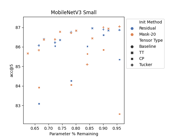
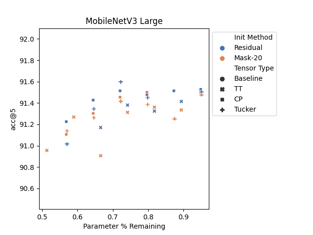
First we compare two variants of our method: additive reconstruction with residual initialization and masking reconstruction with masking initialization. For this experiment, and all other MobileNet experiments, we use SGD with momentum $0.9$ base learning rate $0.1$ and a decay of $0.7$ applied every $5$ epochs. The decay rate was selected using a small grid search over $\{0.5,0.7,0.9\}$ and selecting the best ImageNet-1K validation accuracy for the sparse pruned MobileNet-v3-Large baseline. In Figure 3 we compare the results of our residual initialization strategy with our masking initialization strategy. We observe no clear gains from either strategy. Based on these results we use the simpler residual initialization strategy with additive reconstruction for the remainder of our experiments.

(a)

(b)

Figure 3: Comparison of initialization strategies for low-rank+sparse tensor decomposition for the (a) MobileNet-v3-Small and (b) MobileNet-v3-Large architectures. There are no major distinctions between initialization strategies.

4.2 MobileNetv3 Results

(a)

(b)

(c)

(d)

Figure 4: ImageNet top-5 accuracy comparison between our LR+S method with CP/TT/Tucker tensor format and the sparse pruning baseline. Results for (a) Mobilenet-v3-Small (b) MobileNet-v3-Large (c) EfficientNet-B0 (d) DEIT-Small.

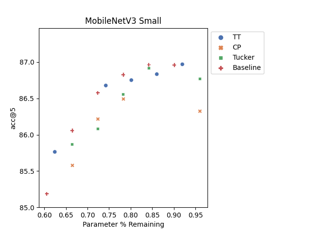
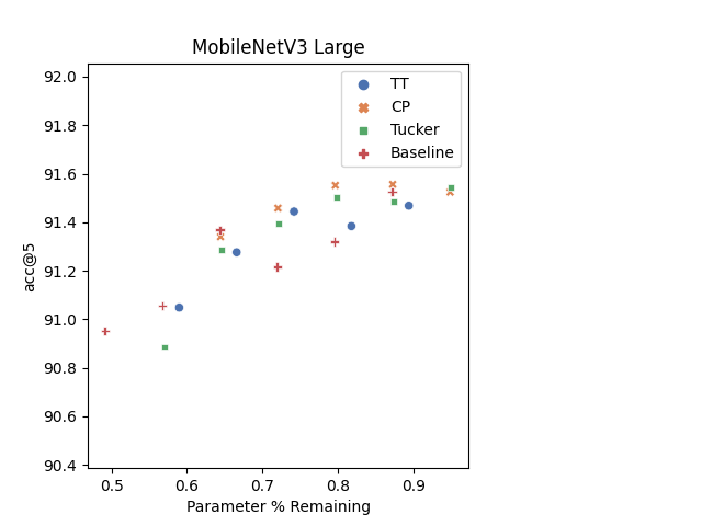
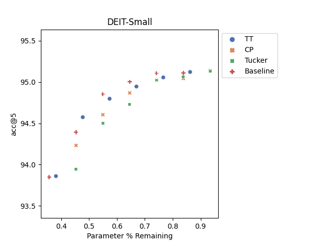
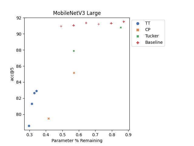
In Figures 4(a) and 4(b) we plot a comparison between our method with varying tensor formats (CP,Tucker,TT) and the sparse pruning baseline on MobileNet-v3-Small and MobileNet-v3-Large respectively. We observe that the combination of low-rank and sparse representations is competitive with the sparse pruning baseline. However we do not observe clear performance advantages.

4.3 Other Models: EfficientNet and DEIT

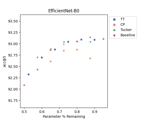
To test if our conclusions hold across architectural families we test on EfficientNet-B0 (Tan & Le, 2019). We use the same optimizer settings as the MobileNet experiments, and report our results in Figure  4(c). We also test our results on DEIT (Touvron et al., 2021) which is a highly accurate Vision Transformer (Dosovitskiy et al., 2020). Specifically, we the the DEIT-Small model with resolution 224 and patch size 16. We train with the Adam optimizer with learning rate $1e-4$. In Figures 4(c) and 4(d) we observe similar results as those from the MobileNet family of models. Low-rank plus sparse decomposition is competitive with sparse pruning across models, but does not significantly outperform sparse pruning.

4.4 Effect on Model Weights

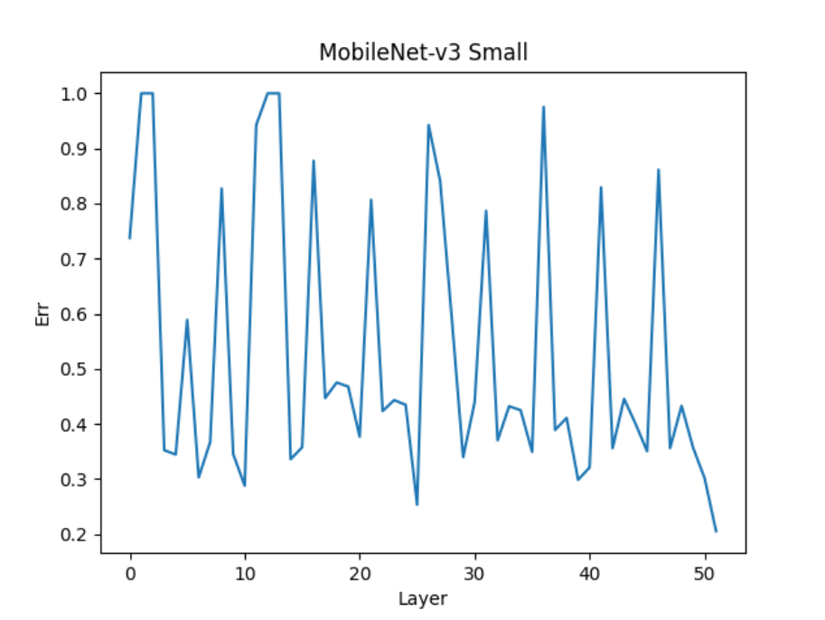
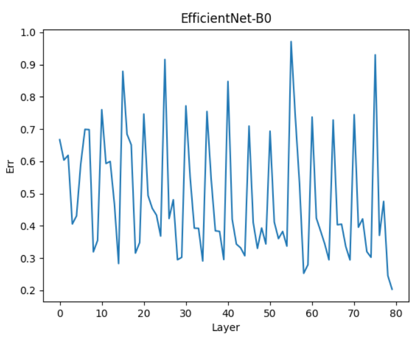
In this section we investigate the effects of our compression methods on the model weights. We highlight a key challenge: many pre-trained models do not possess weights that are close to low-rank. In particular, models with a large number of FC layers or 1x1 convolutions are not “approximately low-rank" even after reshaping from matrix to tensor format. In Figure 5 we plot the layer-wise relative errors of the low-rank decomposition, computed as

$$Err=\frac{\|\mathbfcal{A}-\mathbfcal{L}\|_{2}}{\|\mathbfcal{A}\|_{2}}$$ (15)

We plot the result of CP-format decomposition applied to the MobilNetv3-small and EfficientNet-B0 models. We observe that many layers have a high relative error, but also that several layers stand out in that the low-rank tensor component fits the original tensor $\mathbfcal{A}$ almost exactly.

(a)

(b)

Figure 5: Layer-wise relative error of the low-rank tensor-train factorization for each layer of (a) Mobilenet-v3-Small and (b) EfficientNet-B0. Other tensor types are similar. Layers with high relative error are the pointwise convolutions.

(a) MobileNetv3-Small spatial convolution before and after removing low-rank tensor factors.

(b) Effect of tensor factorization on MobileNetv3-Small spatial convolution weights.

(c) MobileNetv3-Small pointwise convolution before and after removing low-rank tensor factors.

(d) Effect of tensor factorization on MobileNetv3-Small pointwise convolution weights.

Figure 6: (a) Spatial convolutions possess regular structure that can be captured by low-rank tensor factorization. (b) Tensor factorization on spatial convolutions introduces overhead but leads to a weight distribution (in orange) that is easier to prune. (c) Point-wise convolutions posses less regular structure, and tensor factorization induces fewer 0 entries. (d) Tensor factorization on pointwise convolutions introduces overhead and leads to a weight distribution (in orange) that is not easier to prune.

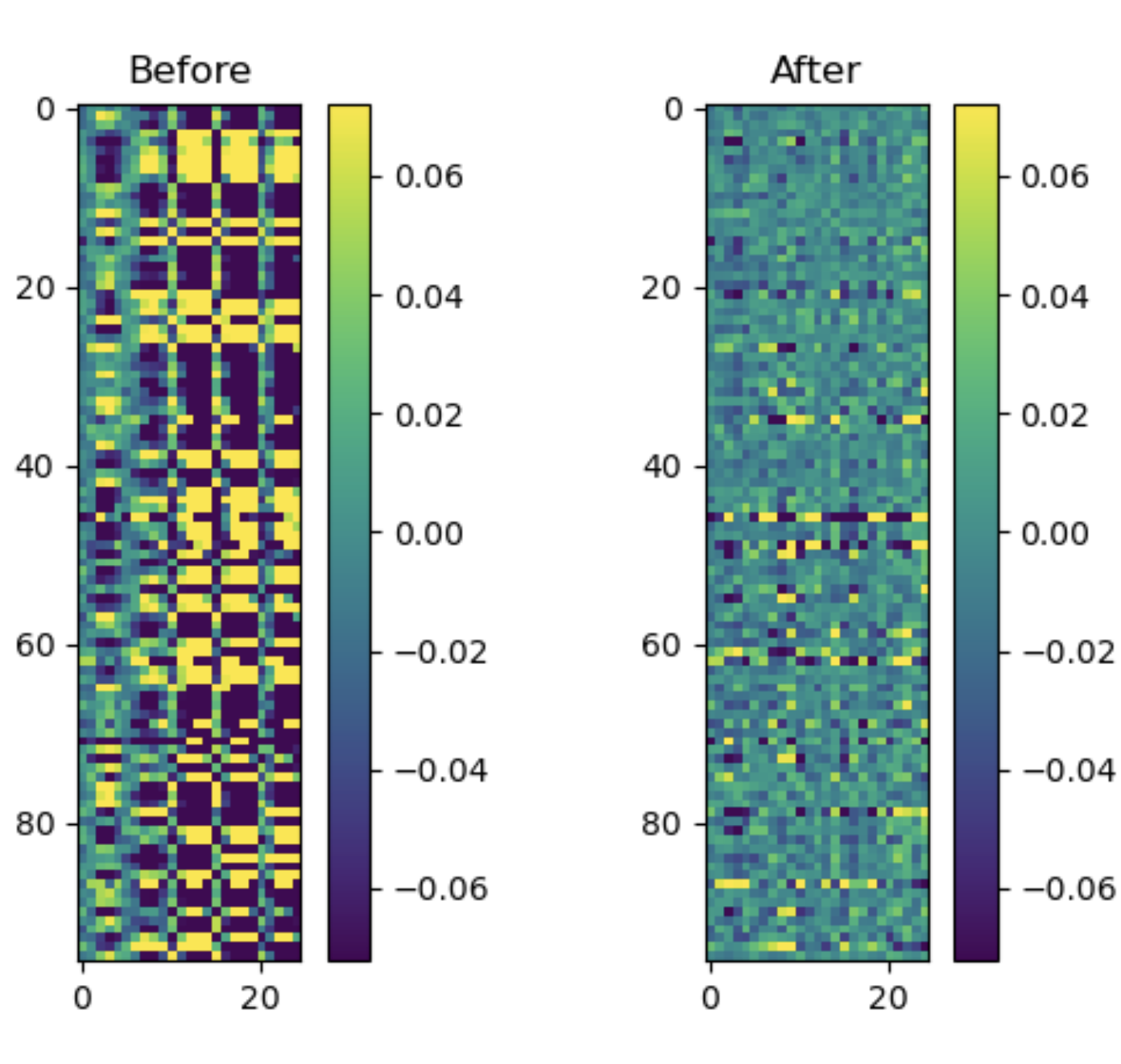
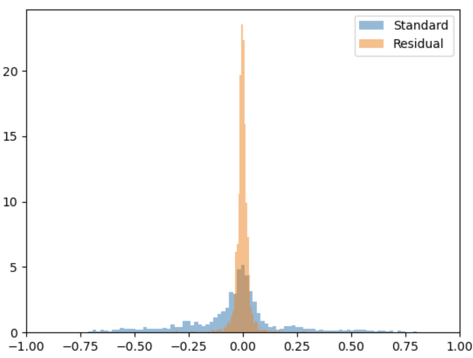
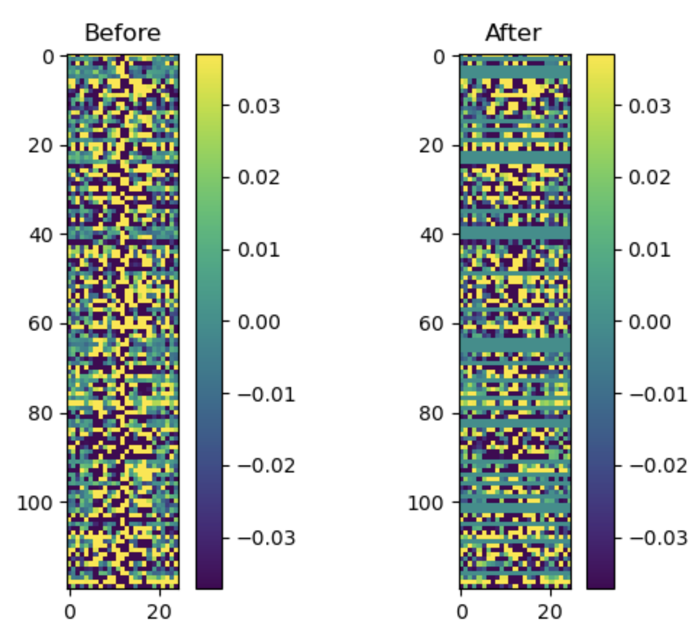
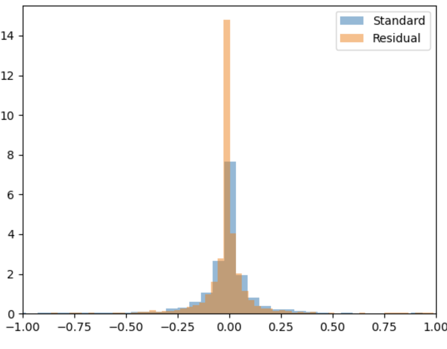
We found that many, but not all, spatial convolutions were fit well by tensor decomposition and have low relative error. We provide an example in Figure 6 which gives representative examples of pointwise and spatial convolutions in MobileNetv3-Small. We detail the effect of our proposed compression method on the model weights. Our motivation is to “preprocess" the weights by removing low-rank structure so that the remaining weight values are better-suited to sparse pruning. Therefore we investigate the effects of our decomposition approach on the weight distributions. We show how tensor compression can remove repeated coarse structure present in spatial convolutions, resulting in a sharply peaked weight distribution compared to the weights of the pretrained model. In contrast tensor decomposition captures less structure in the pointwise convolution and does not induce a weight distribution that is better-suited to sparse pruning.

4.5 Low-Rank Only

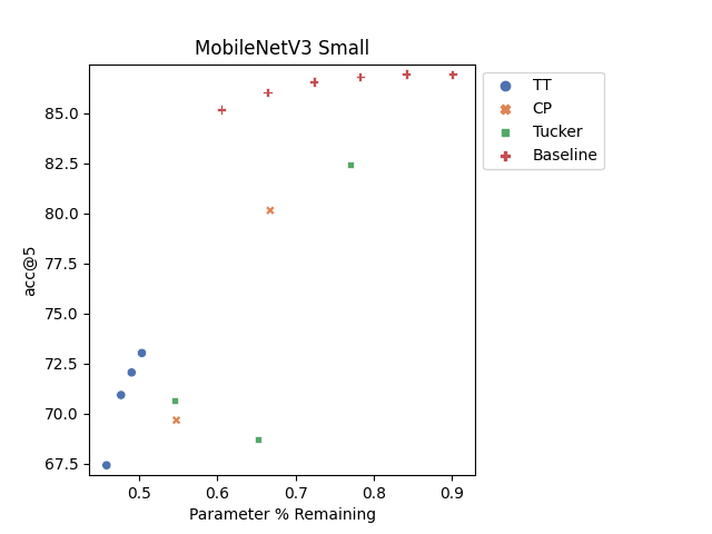
We also considered compressing models using only post-training tensor decomposition. We take a model and perform tensor decomposition on all convolutional kernels and FC layers except the last layer. This idea was first studied in Lebedev et al. (2014) on larger, more compressible architectures. We report our results in Figure 7. We followed the same experimental setup as before, and observed that it was difficult to achieve similar accuracy with low-rank decomposition alone. We hypothesize that this is the natural result of the observation from Figure 5. Since the model weights are not “aproximately low-rank" it is much more challenging to decompose a model and then fine-tune. It is possible that a longer training schedule (>>50 epochs), or training from scratch in low-rank tensor format, would resolve this issue.

(a)

(b)

Figure 7: ImageNet top-5 accuracy comparison between sparse pruning and low-rank tensor decomposition on (a) MobileNet-v3-Small (b) MobileNet-v3-Large

References

- Blalock et al. (2020) Davis Blalock, Jose Javier Gonzalez Ortiz, Jonathan Frankle, and John Guttag. What is the state of neural network pruning? arXiv preprint arXiv:2003.03033, 2020.
- Carroll & Chang (1970) J Douglas Carroll and Jih-Jie Chang. Analysis of individual differences in multidimensional scaling via an N-way generalization of “eckart-young” decomposition. Psychometrika, 35(3):283–319, 1970.
- Cho & Hariharan (2019) Jang Hyun Cho and Bharath Hariharan. On the efficacy of knowledge distillation. In Proceedings of the IEEE/CVF International Conference on Computer Vision, pp. 4794–4802, 2019.
- Deng et al. (2019) Chunhua Deng, Fangxuan Sun, Xuehai Qian, Jun Lin, Zhongfeng Wang, and Bo Yuan. TIE: energy-efficient tensor train-based inference engine for deep neural network. In ISCA, pp. 264–278, 2019.
- Dosovitskiy et al. (2020) Alexey Dosovitskiy, Lucas Beyer, Alexander Kolesnikov, Dirk Weissenborn, Xiaohua Zhai, Thomas Unterthiner, Mostafa Dehghani, Matthias Minderer, Georg Heigold, Sylvain Gelly, et al. An image is worth 16x16 words: Transformers for image recognition at scale. arXiv preprint arXiv:2010.11929, 2020.
- Garipov et al. (2016) Timur Garipov, Dmitry Podoprikhin, Alexander Novikov, and Dmitry Vetrov. Ultimate tensorization: compressing convolutional and FC layers alike. arXiv:1611.03214, 2016.
- Gu et al. (2021) Jiaqi Gu, Hanqing Zhu, Chenghao Feng, Mingjie Liu, Zixuan Jiang, Ray T Chen, and David Z Pan. Towards memory-efficient neural networks via multi-level in situ generation. arXiv preprint arXiv:2108.11430, 2021.
- Gui et al. (2019) Shupeng Gui, Haotao N Wang, Haichuan Yang, Chen Yu, Zhangyang Wang, and Ji Liu. Model compression with adversarial robustness: A unified optimization framework. Advances in Neural Information Processing Systems, 32:1285–1296, 2019.
- Harshman et al. (1994) Richard A Harshman, Margaret E Lundy, et al. PARAFAC: Parallel factor analysis. Computational Statistics and Data Analysis, 18(1):39–72, 1994.
- Hawkins & Zhang (2019) Cole Hawkins and Zheng Zhang. Bayesian tensorized neural networks with automatic rank selection. arXiv:1905.10478, 2019.
- Hawkins et al. (2020) Cole Hawkins, Xing Liu, and Zheng Zhang. Towards compact neural networks via end-to-end training: A bayesian tensor approach with automatic rank determination. arXiv preprint arXiv:2010.08689, 2020.
- Hinton et al. (2015) Geoffrey Hinton, Oriol Vinyals, and Jeff Dean. Distilling the knowledge in a neural network. arXiv:1503.02531, 2015.
- Howard et al. (2019) Andrew Howard, Mark Sandler, Grace Chu, Liang-Chieh Chen, Bo Chen, Mingxing Tan, Weijun Wang, Yukun Zhu, Ruoming Pang, Vijay Vasudevan, et al. Searching for mobilenetv3. In Proceedings of the IEEE/CVF International Conference on Computer Vision, pp. 1314–1324, 2019.
- Howard et al. (2017) Andrew G Howard, Menglong Zhu, Bo Chen, Dmitry Kalenichenko, Weijun Wang, Tobias Weyand, Marco Andreetto, and Hartwig Adam. Mobilenets: Efficient convolutional neural networks for mobile vision applications. arXiv preprint arXiv:1704.04861, 2017.
- Kossaifi et al. (2016) Jean Kossaifi, Yannis Panagakis, Anima Anandkumar, and Maja Pantic. Tensorly: Tensor learning in python. arXiv preprint arXiv:1610.09555, 2016.
- Lebedev et al. (2014) Vadim Lebedev, Yaroslav Ganin, Maksim Rakhuba, Ivan Oseledets, and Victor Lempitsky. Speeding-up convolutional neural networks using fine-tuned cp-decomposition. arXiv:1412.6553, 2014.
- LeCun et al. (1990) Yann LeCun, John S Denker, and Sara A Solla. Optimal brain damage. In NIPS, pp. 598–605, 1990.
- Novikov et al. (2015) Alexander Novikov, Dmitrii Podoprikhin, Anton Osokin, and Dmitry P Vetrov. Tensorizing neural networks. In NIPS, pp. 442–450, 2015.
- Oseledets (2011) Ivan V Oseledets. Tensor-train decomposition. SIAM J. Sci. Computing, 33(5):2295–2317, 2011.
- Sandler et al. (2018) Mark Sandler, Andrew Howard, Menglong Zhu, Andrey Zhmoginov, and Liang-Chieh Chen. Mobilenetv2: Inverted residuals and linear bottlenecks. In Proceedings of the IEEE conference on computer vision and pattern recognition, pp. 4510–4520, 2018.
- Sze et al. (2017) Vivienne Sze, Yu-Hsin Chen, Joel Emer, Amr Suleiman, and Zhengdong Zhang. Hardware for machine learning: Challenges and opportunities. In IEEE Custom Integrated Circuits Conference, pp. 1–8, 2017.
- Tan & Le (2019) Mingxing Tan and Quoc Le. Efficientnet: Rethinking model scaling for convolutional neural networks. In International Conference on Machine Learning, pp. 6105–6114. PMLR, 2019.
- Touvron et al. (2021) Hugo Touvron, Matthieu Cord, Matthijs Douze, Francisco Massa, Alexandre Sablayrolles, and Hervé Jégou. Training data-efficient image transformers & distillation through attention. In International Conference on Machine Learning, pp. 10347–10357. PMLR, 2021.
- Tucker (1966) Ledyard R Tucker. Some mathematical notes on three-mode factor analysis. Psychometrika, 31(3):279–311, 1966.
- Wang et al. (2021) Dilin Wang, Yuan Shangguan, Haichuan Yang, Pierce Chuang, Jiatong Zhou, Meng Li, Ganesh Venkatesh, Ozlem Kalinli, and Vikas Chandra. Noisy training improves e2e asr for the edge. arXiv preprint arXiv:2107.04677, 2021.
- Yang et al. (2020) Lei Yang, Zheyu Yan, Meng Li, Hyoukjun Kwon, Liangzhen Lai, Tushar Krishna, Vikas Chandra, Weiwen Jiang, and Yiyu Shi. Co-exploration of neural architectures and heterogeneous asic accelerator designs targeting multiple tasks. In 2020 57th ACM/IEEE Design Automation Conference (DAC), pp. 1–6. IEEE, 2020.
- Yu et al. (2017) Xiyu Yu, Tongliang Liu, Xinchao Wang, and Dacheng Tao. On compressing deep models by low rank and sparse decomposition. In Proceedings of the IEEE Conference on Computer Vision and Pattern Recognition, pp. 7370–7379, 2017.
- Zhang et al. (May 2021) Kaiqi Zhang, Cole Hawkins, Xiyuan Zhang, Cong Hao, and Zheng Zhang. On-fpga training with ultra memory reduction: A low-precision tensor method. ICLR Workshop of Hardware Aware Efficient Training, May 2021.
- Zhu & Gupta (2017) Michael Zhu and Suyog Gupta. To prune, or not to prune: exploring the efficacy of pruning for model compression. arXiv preprint arXiv:1710.01878, 2017.